Inferring Room Semantics Using Acoustic Monitoring

Abstract

Having knowledge of the environmental context of the user i.e. the knowledge of the users’ indoor location and the semantics of their environment, can facilitate the development of many of location-aware applications. In this paper, we propose an acoustic monitoring technique that infers semantic knowledge about an indoor space over time, using audio recordings from it. Our technique uses the impulse response of these spaces as well as the ambient sounds produced in them in order to determine a semantic label for them. As we process more recordings, we update our confidence in the assigned label. We evaluate our technique on a dataset of single-speaker human speech recordings obtained in different types of rooms at three university buildings. In our evaluation, the confidence for the true label generally outstripped the confidence for all other labels and in some cases converged to 100% with less than 30 samples.

Index Terms—  Indoor Mapping, Room Semantic Inference, Acoustic Monitoring

1 Introduction

During the last decade, location-based services (LBSs) have become evermore pervasive with more than 153 million [1] users relying on their smartphones for directions, recommendations, and other location related information. However, most of these LSBs only function in outdoor environments due to the limitations of the current localization and mapping technologies. Given that Americans spend approximately 90% [2] of their time indoors and that the market for location-based services is projected to exceed $77 billion by 2021 [3], developing systems that would facilitate the development of indoor LBSs is a worthwhile endeavor.

A key per-requisite for developing rich indoor LBSs is the ability to obtain information about the user’s environmental context without any explicit human intervention. The environmental context would include the user’s location within an indoor environment (e.g. second floor, room opposite the elevator) as well as semantic information about the surrounding space (e.g. bathroom). This information could then be used by applications to adapt their behavior, for example, by switching to silent mode if the user is in an auditorium, or automatically declining calls if the user is in the bathroom.

The recent developments in the areas of indoor localization [4, 5, 6, 7, 8] and indoor mapping [9, 10, 11] have made it possible to generate accurate indoor floor plans and track users as they move within them. However, these floor plans are largely devoid of any semantic labels for the comprising spaces and therefore have limited usefulness. A few works have attempted to leverage multiple data sources such as wireless signals, sound, light and sensor data to associate semantic meanings with indoor locations [12, 13] while others have tried to leverage social-network data, such as check-ins, to annotate unlabeled floor plans with semantic labels [14]. The infrastructure requirements and training overheads of these approaches limit their feasibility to be deployed as part of a ubiquitous system.

To offer a more robust, scalable, and practical technique for inferring the semantics of indoor spaces, we have chosen to rely on audio recordings obtained from these spaces. While there are several other modalities that can be employed for this purpose, including wireless signals and images, certain properties of audio signals make them particularly convenient to be used in this context. Audio data is easy to collect, process, and store due to the popularity of handheld devices sporting high quality recording hardware, and low bandwidth of the audio signal. Furthermore, audio signals are relatively invariant to changes in the position and orientation of the recording device, and unlike visual data, are not limited by ambient lighting conditions. More significantly, audio signals carry potentially discriminative signatures of the environment they were recorded in. These characteristics make sound well suited as a modality to be incorporated in a lightweight semantic inference system.

In this paper, we propose an acoustic monitoring technique that infers semantic knowledge about an indoor space by collecting and analyzing audio recordings from it over time. Current approaches for extracting semantic information present in the acoustic forensics [15] and scene classification [16, 17, 18] literature predominantly rely on performing one-off classification in which each individual data sample is classified independently. Meanwhile, our approach to this problem is fundamentally different, and to the best of our knowledge, has not been explored in the current literature. We treat individual audio samples as evidence to help us infer a semantic label for the environment it was obtained from. Like in a forensic investigation, a single piece of evidence is of limited significance. As part of a robust investigative process, all the evidence must be aggregated for inferences to be drawn from it. As we obtain and analyze more samples we accumulate more evidence and our confidence in the label we inferred for the space increases. Summarizing the novelty of our approach, when analyzing an audio recording, the current approaches try to answer the question “where was this recorded?”, whereas we ask a different question altogether, i.e. “given this recording, and $n$ recordings that we had received earlier from the same place, how likely is it that this place is, for example, an office?”.

For inferring the semantics of a space, our technique uses appropriate models to extract and combine evidence from two acoustic characteristics of the space, namely, ambient sounds and the impulse response. We use Mel-Frequency Cepstral Coefficients (MFCCs) to model the ambient soundscape. While, on the other hand, we use a non-negative de-convolution approach to isolate the Room Impulse Response (RIR). We then use Gaussian Mixture Models (GMM) and Support Vector Machines (SVMs) to classify the MFCCs and RIR respectively . We find that both of these characteristics are capable of independently providing confirmation of the semantics of a space. Moreover, we also find that combining evidence from both yields significantly better performance than either of the characteristics alone. As mentioned above, our approach incrementally builds up confidence in the classification of a room over time from the accumulated evidence of multiple recordings. It does so by aggregating the evidence provided by our models using Bayesian inference.

We evaluated our approach on a large dataset of audio recordings. We collected over 12,000 recordings from five different types of room in three university buildings using smartphones. Our technique was able to correctly identify all the room types when the training and testing data came from the same set of buildings. When tested on an unseen building it only misclassified one room type. In our evaluations, our technique was able to reach 100% classification confidence with as less as 30 recordings.

The remainder of the paper is organized as follows, section 2 presents the feature extraction techniques and learning models we have used, section 3 presents the evaluation process and the results and the discussion in section 4 ends the paper.

2 Inferring Room Semantics from Audio

Our objective is to automatically detect room semantics – the purpose of any room – from audio recordings within that room. Audio signals have a convenient property of being able to capture potentially discriminatory information about the environment. From a purely acoustic perspective, environments, rooms in our case, can differ along two dimensions: (1) The acoustic content, that characterizes the typical sounds in the room and (2) the room impulse response, which characterizes its structure.

Our approach employs different pre-processing and classification strategies to exploit each of these characteristics and combine them for our final decision. We extract MFCCs from the audio recordings then use GMMs to model the ambient soundscape present in each room type. We also extract the RIR from the Short-Time Fourier Transform (STFT) using the non-negative deconvolution approach below. We parameterize the RIR and use it to train SVM classifiers for each room type. Finally, we must also consider that a room may serve multiple purposes. For instance, a pantry may double as a printer room in an office building. Thus, rather than attempting to classify between multiple semantic options, we will treat the problem as one of detection, applied to each semantic. The decision is not intended to be instantaneous; rather, we will attempt to determine the confidence with which each semantic may be assigned to the room incrementally, from recordings obtained over time. As a result, we require a higher-level framework within which evidence is combined to incrementally build up confidence in the label attributed to the room.

We describe each of the components of our procedure below.

2.1 Classifying by Acoustic Content

Ambient sounds can be used to qualitatively differentiate a room. These ambient sounds can be thought of as composing an acoustic scene that is intrinsically linked to some high-level semantic of the space. For example, the sound of water splashing is a characteristic of the bathroom, while a kitchen space may be expected to contain the sounds of appliances humming.

We cast the problem of identifying a room type as one of acoustic scene classification [19]. In modeling the ambient sound scene, the temporal arrangement of sound patterns is not of particular significance, rather what we are interested in is capturing the qualitative features of the sound scene. While a number of techniques have been proposed for this purpose in the literature [19, 20, 21], in our work we have chosen to use a Gaussian mixture classifier. We do so because it has been shown that the qualitative features of an acoustic scene can be effectively modeled by the distribution of frame-based spectral features [22]. Furthermore, this approach also enables us to compute log-likelihoods, which is convenient for subsequent calculations.

For each room type $C$ we model the distribution of Mel-Frequency Cepstral vectors derived from acoustic recordings in instances of that room as a Gaussian mixture:

$$p(\vec{x}|C)=\sum_{i=1}^{N}w_{C,i}{\mathcal{N}}(\vec{x};\mu_{C,i},\Sigma_{C,i})$$ (1)

, where $\vec{x}$ represents a random cepstral vector, ${\mathcal{N}}(\vec{x};\mu,\Sigma)$ represents a Gaussian distribution for $\vec{x}$ with mean $\mu$ and variance $\Sigma$, $N$ represents the number of Gaussians in the mixture, and $w_{C,1},\cdots,w_{C,N}$ are the weights of the Gaussians in the mixture. Similarly, the probability density function of vectors from recordings that do not belong to the room are also modeled by a Gaussian mixture obtained by replacing $C$ by $\neg C$ in equation (1) where $\neg C$ is the set of all rooms types except $C$. The parameters of both distributions (namely the mixture weights, means, and variances) are learned from training instances of recordings using the expectation-maximization algorithm [23].

Given a test recording $\mathbf{X}=\vec{x}_{1},\cdots,\vec{x}_{T}$, we compute the within class and out-of-class log likelihoods as $L_{A}(\mathbf{X}|C)=\sum_{t}\log p(\vec{x}_{t}|C)$, and $L_{A}(\mathbf{X}|\neg C)=\Sigma_{t}\log p(\vec{x}_{t}|\neg C)$. Classification may be performed by directly comparing $L_{A}(\mathbf{X}|C)-L_{A}(\mathbf{X}|\neg C)$ to a threshold. We will, however, use these values to compute confidences as explained below.

2.2 Room Impulse Response Extraction and Classification

The purpose of a room is also reflected in the size, shape, and furnishings of the room. These, in turn, will affect the Room Impulse Response of the room. For instance, the reverberation times and the room response of bathrooms, which are generally small-to-mid sized, devoid of furniture, and often have hard reflective surfaces such as tiles and mirrors, will be very different from those of a class room with tables, chairs, and (usually) people occupying them, and these in turn will be different from offices with their very different form factors and furnishings.

In order to exploit this information to classify rooms, however, it will be necessary to derive the room response from the recordings, parametrize them appropriately, and utilize an appropriate classifier. We discuss our approach below.

2.2.1 Extracting Room Impulse Response

Extracting exact room responses from a monaural recording remains a challenging and unsolved problem. However, for our purposes, an approximate estimate obtained from general principles will suffice. We use the non-negative deconvolution method described in [24] for our purpose.

Following the approach of [24], we model the effect of the room on the acoustic signal as a convolution of the magnitude spectrogram of the signal with the magnitude spectrogram of the room impulse response. The room impulse response is then extracted from the magnitude spectrogram of the reverberant recorded signal through non-negative matrix deconvolution.

Given an observed signal, represented by a $F\times T$ magnitude-spectrogram matrix, $\mathbf{X}$, (where $T$ represents the number of time frames and $F$ is the number of frequency bands), our goal is to approximate $F\times T$ matrix, $\mathbf{S}$ and $F\times K$ matrix $\mathbf{R}$, such that $\mathbf{Y=S*R}$ and $\mathbf{Y\simeq X}$, $*$ represents the convolution operation and, $\mathbf{S}$ and $\mathbf{R}$ represent the magnitude spectrograms of the speech and RIR respectively.

We define $F\times F$ matrices $\mathbf{R}_{1},\ldots,\mathbf{R}_{K}$ such that

$$\mathbf{R}_{k}=diag(R_{1}[k],...,R_{F}[k])$$

where $\mathbf{R}_{k}$ is a diagonal matrix with $R_{1}[k],...,R_{F}[k]$ as the values on the diagonal and $R_{f}[t]$ represents the magnitude spectral component of the $f^{th}$ frequency sub-band at time index $t$ for the RIR. Now we can formulate the approximation as

$$\mathbf{Y=\sum_{\text{$k=1$}}^{\text{$K$}}R_{\text{$k$}}\cdot\overset{\text{$k\rightarrow$}}{S}}.$$

where $k\rightarrow$ represents a right shift of the spectrogram by $k$ time steps. Since we are dealing with speech, $\mathbf{S}$ needs to be sparse. To encourage sparsity we use the update rule for $\mathbf{S}$ presented in [24], which introduces sparsity parameters $p$ and $\lambda$. The update rules for $\mathbf{S}$ and $\mathbf{R}$ are

$$\mathbf{S}\leftarrow\mathbf{S}\otimes\dfrac{\mathbf{\sum_{\text{$k=1$}}^{\text{$K$}}R_{\text{$k$}}\cdot\overset{\text{$k\leftarrow$}}{X}}}{\mathbf{\lambda}|\mathbf{S}|^{p-1}+\mathbf{\sum_{\text{$k=1$}}^{\text{$K$}}R_{\text{$k$}}\cdot\overset{\text{$k\leftarrow$}}{Y}}}$$

$$\mathbf{R_{\text{$k$}}=R_{\text{$k$}}\otimes\dfrac{\dfrac{X}{Y}\cdot\overset{\text{$k\rightarrow$}}{S}^{\top}}{1\cdot\overset{\text{$k\rightarrow$}}{S}^{\top}}},$$

where $\otimes$ represents the Hadamard product. After the procedure has converged we reconstruct a $F\times K$ matrix, $\mathbf{R}$ representing the RIR by placing the diagonal of $\mathbf{R}_{k}$ at the $k^{\text{th }}$ column of $\mathbf{R}$.

2.2.2 Parametrizing and Classifying the RIR

The outcome of the above procedure is a $F\times K$ matrix representing the magnitude spectrogram of the RIR. Note that although the actual RIR of any room is infinite in length, our estimates returns a finite and fixed-length RIR; this approximation enables us to obtain fixed- and finite-length characterizations that we can use for classification.

We compress the RIR further by taking the logarithm of the magnitude spectra and performing a Discrete Cosine Transform (DCT) on individual rows. We only keep the first 20 cepstral features from the DCT, so that we are left with a $20\times K$ matrix for the RIR. Since the temporal pattern represented by the arrangement of the rows is significant we simply flatten this matrix to obtain a $20K$-dimensional feature vector. Note that this way we retain the entire RIR as a feature and in doing so we account for the temporal structure of the audio frames in the RIR.

To classify the RIR, we use Support Vector Machines (SVMs). We chose SVMs, instead of using distribution models such as i-vectors or GMMs, for this task because, unlike the acoustic scene, classifying RIR requires us to explicitly account for the temporal variations in the signal, making distribution-based method unsuitable. We setup the SVM to map the classification scores to values between 0 and 1 and can be interpreted as probabilities. Let $L_{R}(\mathbf{X}|C)$ and $L_{R}(\mathbf{X}|\neg C)$ represent the log probabilities assigned to $C$ and $\neg C$ by the SVM. In order to classify the RIR, we can compare the difference of the two log probabilities to a threshold; however, as in the case of scene classification described above, we will use them to compute confidences.

2.3 Incremental Confidence Calculation

Finally, we compose the results from the individual recordings to obtain an incrementally updated confidence value for each room type $C$. In principle, these could be computed directly through iterated computation of a posteriori probabilities of the classes via Bayes rule using the original probability values obtained from the GMMs and SVM. Instead, we employ the approach described in [25] as we find it to be more effective.

First we combine the results from the GMMs and SVMs into a hybrid model. Each model is designed to capture a specific set of features from the recordings so relying exclusively on one of them may lead to potentially relevant information being discarded. While on the other hand by combining the two classifiers we stand to benefit from the unique information captured by each model. For each recording, $\mathbf{X}$, we compute log-likelihood ratio scores, $\mathbf{L}_{A}=L_{A}(\mathbf{X}|C)-L_{A}(\mathbf{X}|\neg C)$ and $\mathbf{L}_{R}=L_{R}(\mathbf{X}|C)-L_{R}(\mathbf{X}|\neg C)$, from the acoustic scene and RIR classifiers respectively. We then compute a single overall log-likelihood ratio score given by

$$p_{i}=\alpha(\mathbf{L}_{A})+(1-\alpha)(\mathbf{L}_{R})$$ (2)

where $\alpha$ weighs the contribution of the acoustic scene classifier in the overall score. Let $p_{i}^{\prime}=p_{i}-t_{C}$ where $t_{C}$ is a constant threshold value. Define $P(p_{i}^{\prime}|C)$ and $P(p_{i}^{\prime}|\neg C)$ to be the distributions of the $p_{i}^{\prime}$ values for $C$ and $\neg C$. In practice we set $t_{C}$ to be the threshold value at which the False Positive Rate (FPR) equals the False Negative Rate (FNR) for class $C$. This value of FPR and FNR is known as the Equal Error Rate (EER). Following [25] we model both as Gaussian Mixtures, the parameters of which can be trained from training data. Given a sequence of observations $p_{1},\cdots,p_{n}$ and the respective $p_{i}^{\prime}$, the incremental confidence update rule is given by

$$P(C|p_{1}^{\prime},\cdots,p_{n}^{\prime})=\frac{\Pi_{i}^{n}P(p_{i}^{\prime}|C)}{\Pi_{i}^{n}P(p_{i}^{\prime}|C)+\omega\Pi_{i}^{n}P(p_{i}^{\prime}|\neg C)}$$ (3)

where $\omega$ is a constant that represents $\dfrac{P(\neg C)}{P(C)}$.

3 Evaluation

3.1 Dataset

We have compiled a data set comprising over 12,004 speech recordings for our experiments. The speech is recorded by two smartphones simultaneously over a single channel at a sampling rate of 44.1 Khz. A Samsung Galaxy SIII mini is held by the speaker at chest level, while a Sony Xperia Z1 Compact is in his pocket. The recordings were performed in several Bathrooms(BR), Offices(O), Pantries(P), Classrooms(C) and Lecture Halls (LH) on three university buildings (referred to as C-I, C-II and C-III below). In each room we took 100 recordings, 3 seconds each. The speaker stood at 5 locations within the room and uttered 4 short sentences, repeating each sentence 5 times. The recordings were obtained at times when there was low foot traffic in order to keep them as clean as possible.

For the experiments in this paper, we use only the recordings from the aforementioned dataset in which the smartphone was held up by the speaker, since the recordings obtained with the phone kept in the speaker’s pocket could not have effectively captured the RIR.

We divide the data into four folds for cross-validation. All experimental results reported below have been averaged over the 4 folds. The folds are constructed such that no two folds have data from the same room in order to ensure that the training set does not have any data from the rooms in the test set.

3.2 Feature Extraction

We extract two feature sets from the raw audio signal, Mel-Frequency Cepstral Coefficients (MFCCs) and the RIR. For both, we compute the Short Time Fourier Transform (STFT) using a 64ms hamming window with 32ms overlap. To model ambient sound we compute 20-dimensional MFCCs, extended with difference coefficients [26]. To extract the parameterized RIR we apply the NMFD based de-reverberation procedure described earlier to STFT.

3.3 Training

For scene classification we train two Gaussian mixtures, each having 64 components, per room type. One mixture is trained on the data for the specific room type while the other is trained on the data from all other room types. To classify the RIRs, we trained a binary SVM with a radial-basis function (RBF) kernel for each room type using LIBSVM[27]. We setup the SVM to output probability values for the positive and negative classes and used grid search with five fold cross-validation to find the optimal parameters for the SVM.

3.4 Results

3.4.1 Classifier Evaluation

Room Type	Scene	RIR
Lecture Hall	8.72	13.53
Classroom	12.23	34.03
Pantry	10.68	22.05
Office	6.42	23.23
Bathroom	8.2	5.5

Table 1: EER, acoustic scene classification.

We first evaluate room classification performance on individual recordings obtained from campuses C-I and C-II, using the equal error rate (EER) as the metric. It is important to note that while the testing and training set do not have data from the same rooms, they do have data from the same set of buildings. The EERs for the acoustic scene and RIR classifiers are given in Table 1. While both classifiers produced encouraging results, the acoustic scene classifier outperformed the RIR classifier in all room types except for the bathrooms suggesting that the acoustic scene is well suited for characterizing rooms of different types. Though less impressive than the acoustic scene classifier, the results from the RIR classifier are still quite good. The RIR classifier performs very well on environments with distinctive structural features, namely lecture halls and bathrooms. The high ceilings of lecture halls and the ceramic tiling in the bathrooms would produce acoustic artifacts which are not found in other types of rooms. However, we see that structural information alone, as obtained from the RIR, may not be sufficient when trying to classify more complex acoustic environments such as classrooms, offices and pantries. With that said, we still maintain that the structural information captured by the RIR is salient in the semantic inference process. As we shall see in the next section, augmenting the acoustic scene classifier with the structural information from the RIR yield significantly better classification performance.

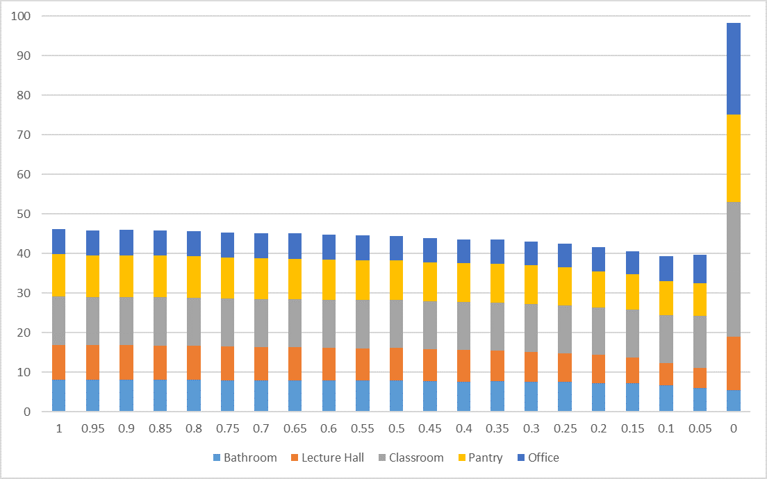
Fig. 1: Total EER as $\alpha$ is varied. Each color represents one type of room.

3.4.2 Combining The Classifiers

As we stated in 2.3, we want to aggregate the information obtained from both, the acoustic scene and the RIR classifiers into a hybrid model using equation (2). We empirically determine the optimal value of the weight parameter $\alpha$ in equation (2) by computing the total EER, across all room types, for different values of $\alpha$ and choosing the $\alpha$ at which the total EER is minimized.

Fig.1 illustrates how the total EER decreases as $\alpha$ is varied. The EER decreases as $\alpha$ is decreased reaching a minimum at $\alpha=0.10$. In fact, the total EER obtained by combining the classification results, with $\alpha=0.10$, is 14.7% lower than that of the audio scene classifier ($\alpha=1.0$) and 59.9% lower than that of the RIR classifier ($\alpha=0.0$). This observation is quite interesting because the RIR classifier alone yields very high error rates but by providing just a little information from the acoustic scene classifier we can drastically reduce them and obtain better performance than the acoustic scene classifier itself.

3.4.3 Confidence Calculation

We evaluate the ability of the proposed approach to incrementally buildup confidence in semantic labels for the rooms. Given a set of recordings, all obtained from within the same room, we use the Bayesian inference procedure described in 2.3 to incrementally update our confidence in the candidate semantic labels for the given room. As more audio samples are made available to the classifier we expect to see the confidence in the true label increase while the confidence in other labels diminishes. In our experiments we set $\omega=4$ and, model $P(p_{i}^{\prime}|C)$ and $P(p_{i}^{\prime}|\neg C)$ as a four component Gaussian mixture. Figure 2 illustrates the process of confidence build up on the data from campuses C-I and C-II when classified using the hybrid model with $\alpha=0.10$.

It is encouraging to see that our technique can confidently infer the correct semantic label for different room types given a set of audio recordings. For all the room types in our dataset, our confidence in the true label clearly outstripped our confidence in all other labels. For three out of five room types the confidence in the true label rapidly approached 100%, with less than 30 samples and thereby demonstrating the practical viability of our proposed approach. By far the most impressive performance was shown by bathrooms which were unambiguously labeled with 100% confidence with less than a handful of recordings. The performance was not as impressive for lecture halls but confidence in the true label still converged to more than 75% with less than 20 samples, while the confidence for all other labels remained much lower.

Another interesting consequence of our technique is that the confidence values for different rooms are not correlated. This permits our technique to accurately represent situations in which a room serves multiple purposes and needs to be assigned more than one semantic tag or, if the room is of a type that is not known to our classifier, to be flagged as unknown.

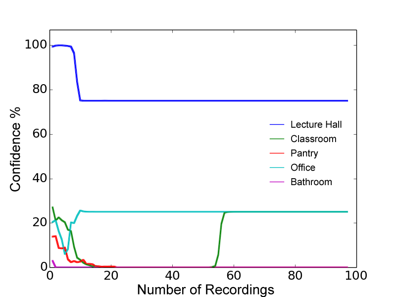
(a) Lecture Halls

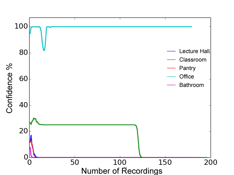
(b) Offices

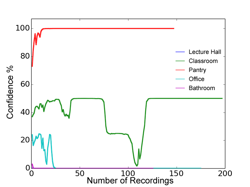
(c) Pantries

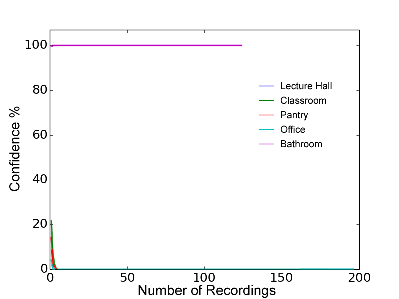
(d) Bathrooms

Fig. 2: Confidence build up per room using the hybrid classifier with $\alpha=0.10$

3.4.4 Testing On An Unseen Building

While the results in Fig. 2 are very encouraging they are not conclusive because the rooms in the training and testing set come from the same set of building. It is very common for rooms of a particular type in the same buildings to be homogeneous in their structure and layout. This homogeneity can lead to similar acoustic features being observed in these rooms. Therefore, we run the risk of our models over-fitting to these common features and producing overly optimistic results.

To obtain a more reliable set of results we evaluate our technique on an “unseen” building i.e. a building not included in the training set. We train our classifiers using the data from the campuses C-I and C-II and test on the data from the campus C-III. We use the hybrid classification model with $\alpha=0.10$ and calculate confidence using equation (3) with thresholds, $t_{C}$, set to threshold values corresponding to the EER values in Table 1. Due to space considerations we have chosen to only illustrate the final confidence values for each label in the form of a confusion matrix presented in Fig.3.

Notwithstanding the fact that our training dataset only had data from two buildings and hence was lacking in diversity, our technique was able to correctly infer the labels for four out of the five room types in our dataset. We were able to confidently label lecture halls, bathrooms and offices. While we were absolutely certain about our labels for the offices and bathrooms, the lecture halls were being confused with classrooms in some cases. This is not a serious setback since lecture halls and classrooms can have a lot of similar features and their structural layout can vary significantly across different buildings. However, our technique was not very sure about the label for pantries and grossly miss-classified the classrooms. We believe that these errors were caused by the fact that the classrooms and pantries in the test building significantly differed in their layout and content from their counterparts in the training buildings. Unlike the training classrooms, the classrooms in the test buildings also served as computer clusters while the pantries in the test building were significantly smaller than the ones in the training set and lacked certain appliances such as printers. These differences would probably have changed the ambient sound patterns present in the rooms as well the impulse response.

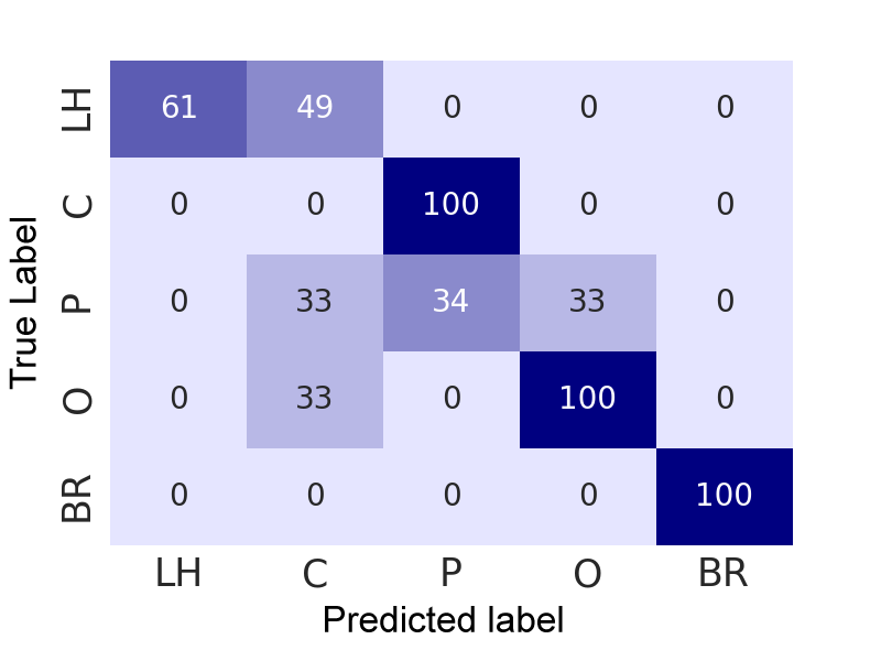
Fig. 3: Confusion Matrix of final classification confidence values on the unseen building.

4 Conclusion

We have proposed an acoustic monitoring scheme to detect room semantics from audio recordings. We have demonstrated that both qualitative (ambient sound scene) and structural (RIR) identifiers of spaces are capable of providing confirmation of a room’s semantic label, however, a linear combination of the two classifiers yields lower error rates than each classifier achieved individually. We have also developed a Bayesian inference technique for aggregating the evidence obtained from the classifiers to build up confidence in semantic labels for rooms over time. Finally we have evaluated our system using audio recorded in three university buildings. On the validation dataset, consisting of data from two campuses, the confidence of our system in the true label significantly outstripped its confidence in all other labels. Moreover, our system also performed very well on the data from the third campus, that was not included in a training set, assigning correct labels to 4 out of 5 different classes of rooms.

The work presented in this paper is part of a larger project to create a lightweight crowdsourced system for automated annotation of indoor floorplans, in which audio is one of the modalities, along with visual and sensory data, to be employed to infer the semantic labels for rooms. As future work, we plan on performing evaluation trials with volunteers. We intend to make all the data we gather available to the public to facilitate future work in this area.

References

- [1] “Location-based services and real time location systems market by location (indoor and outdoor), technology (context aware, uwb, bt/ble, beacons, a-gps), software, hardware, service and application area - global forecast to 2021,” .
- [2] “The national human activity pattern survey (nhaps): a resource for assessing exposure to environmental pollutants,” Journal of Exposure Science and Environmental Epidemiology, vol. 11, no. 3, pp. 231, 2001.
- [3] “Most smartphone owners use location-based services,” Apr 2016.
- [4] Swarun Kumar and et al., “Accurate indoor localization with zero start-up cost,” in Proc. MobiCom. ACM, 2014, pp. 483–494.
- [5] Robert W Levi and Thomas Judd, “Dead reckoning navigational system using accelerometer to measure foot impacts,” Dec. 10 1996, US Patent 5,583,776.
- [6] Paramvir Bahl and Venkata N Padmanabhan, “Radar: An in-building rf-based user location and tracking system,” in Proc. INFOCOM 2000. IEEE, 2000, vol. 2, pp. 775–784.
- [7] Abderrahmen Mtibaa, Khaled A Harras, and Mohamed Abdellatif, “Exploiting social information for dynamic tuning in cluster based wifi localization,” in Wireless and Mobile Computing, Networking and Communications (WiMob), 2015 IEEE 11th International Conference on. IEEE, 2015, pp. 868–875.
- [8] Mohamed Abdellatif, Abderrahmen Mtibaa, Khaled A Harras, and Moustafa Youssef, “Greenloc: An energy efficient architecture for wifi-based indoor localization on mobile phones,” in Communications (ICC), 2013 IEEE International Conference on. IEEE, 2013, pp. 4425–4430.
- [9] Moustafa Alzantot and Moustafa Youssef, “Crowdinside: automatic construction of indoor floorplans,” in Proc. SIGSPATIAL. ACM, 2012, pp. 99–108.
- [10] Ruipeng Gao and et al., “Jigsaw: Indoor floor plan reconstruction via mobile crowdsensing,” in Proc. MobiCom. ACM, 2014, pp. 249–260.
- [11] Ahmed Saeed, Ahmed Abdelkader, Mouhyemen Khan, Azin Neishaboori, Khaled A Harras, and Amr Mohamed, “Argus: realistic target coverage by drones.,” in IPSN, 2017, pp. 155–166.
- [12] Xuan Bao and et al., “Pinplace: associate semantic meanings with indoor locations without active fingerprinting,” in Proc. Ubicomp. ACM, 2015, pp. 921–925.
- [13] Martin Azizyan and et al., “Surroundsense: mobile phone localization via ambience fingerprinting,” in Proc. MobiCom. ACM, 2009, pp. 261–272.
- [14] Moustafa Elhamshary and Moustafa Youssef, “Semsense: Automatic construction of semantic indoor floorplans,” in Proc. IPIN, 2015. IEEE, 2015, pp. 1–11.
- [15] Hong Zhao and Hafiz Malik, “Audio recording location identification using acoustic environment signature,” IEEE Transactions on Information Forensics and Security, vol. 8, no. 11, pp. 1746–1759, 2013.
- [16] Keansub Lee and et al., “Detecting local semantic concepts in environmental sounds using markov model based clustering,” in ICASSP, 2010, pp. 2278–2281.
- [17] Toni Heittola, “Detection and classification of acoustic scenes and events 2016,” .
- [18] Robert G Malkin and Alex Waibel, “Classifying user environment for mobile applications using linear autoencoding of ambient audio,” in ICASSP, 2005, vol. 5, pp. v–509.
- [19] Daniele Barchiesi and et al., “Acoustic scene classification: Classifying environments from the sounds they produce,” IEEE Signal Processing Magazine, vol. 32, no. 3, pp. 16–34, 2015.
- [20] Jurgen T Geiger and et al., “Large-scale audio feature extraction and svm for acoustic scene classification,” in IEEE Workshop on Applications of Signal Processing to Audio and Acoustics, 2013, pp. 1–4.
- [21] Dimitrios Giannoulis and et al., “Detection and classification of acoustic scenes and events: An ieee aasp challenge,” in IEEE Workshop on Applications of Signal Processing to Audio and Acoustics, 2013, pp. 1–4.
- [22] Jean-Julien Aucouturier and et al., “The bag-of-frames approach to audio pattern recognition: A sufficient model for urban soundscapes but not for polyphonic music,” The Journal of the Acoustical Society of America, vol. 122, no. 2, pp. 881–891, 2007.
- [23] Arthur P Dempster and et al., “Maximum likelihood from incomplete data via the em algorithm,” Journal of the royal statistical society. Series B (methodological), pp. 1–38, 1977.
- [24] Hirokazu Kameoka and et al., “Robust speech dereverberation based on non-negativity and sparse nature of speech spectrograms,” in ICASSP, 2009, pp. 45–48.
- [25] Rita Singh and Bhiksha Raj, “Classification in likelihood spaces,” Technometrics, vol. 46, no. 3, pp. 318–329, 2004.
- [26] Douglas A Reynolds and Richard C Rose, “Robust text-independent speaker identification using gaussian mixture speaker models,” IEEE transactions on speech and audio processing, vol. 3, no. 1, pp. 72–83, 1995.
- [27] Chih-Chung Chang and Chih-Jen Lin, “Libsvm: a library for support vector machines,” TIST, vol. 2, no. 3, pp. 27, 2011.