Abstract

In this paper, we develop a low-order three-dimensional finite-element solver for fast multiple-case crust deformation computation on GPU-based systems. Based on a high-performance solver designed for massively parallel CPU-based systems, we modify the algorithm to reduce random data access, and then insert OpenACC directives. By developing algorithm appropriate for each computer architecture, we enable to exhibit higher performance. The developed solver on ten Reedbush-H nodes (20 P100 GPUs) attained speedup of 14.2 times from the original solver on 20 K computer nodes. On the newest Volta generation V100 GPUs, the solver attained a further 2.52 times speedup with respect to P100 GPUs. As a demonstrative example, we computed 368 cases of crustal deformation analyses of northeast Japan with 400 million degrees of freedom. The total procedure of algorithm modification and porting implementation took only two weeks; we can see that high performance improvement was achieved with low development cost. With the developed solver, we can expect improvement in reliability of crust-deformation analyses by many-case analyses on a wide range of GPU-based systems.

1 Introduction

Simulations reflecting the physical phenomena of earthquake disasters are useful for gaining knowledge on earthquake disaster processes and improve estimation accuracy for future earthquakes. As the target domain of earthquake disaster simulations is heterogeneous and involves complex geometry, large-scale implicit three-dimensional (3D) finite-element analysis using low-order unstructured elements is suitable. In such simulations, most of the computing cost is spent in solving a large system of linear equations. Thus, we have been developing fast solver algorithms for CPU-based systems; our solvers GAMERA and GOJIRA running on the massively parallel CPU-based K computer system [1] were nominated as Gordon Bell Prize finalists in SC14 and SC15 [2], [3]. Furthermore, we ported this solver to GPU environments using OpenACC [4] , which was presented at the Workshop on Accelerator Programming Using Directives (WACCPD) 2016 [5]. This enabled further acceleration and use on wider computing environments with low additional development cost.

Although very challenging, forecasting of the time, position, and magnitude of an earthquake is one of the major goals in earthquake science and disaster mitigation. One promising means of such forecasting could be physics-based forecasting that uses GPS observation data of crust-deformation and many-case analyses to estimate plate boundary states via inverse analyses. In these analyses, many cases of 3D finite-element simulations for each slip distribution are required. Thus, the required computing cost increases significantly when compared with single case finite-element simulations. To deal with the increased computational costs, an algorithm that is specialized for crust-deformation analysis has been developed based on GAMERA [6]. This solver enabled 2.18 times speedup on crust-deformation problems on the K computer when compared with GAMERA. Porting this solver to GPU-based systems using OpenACC can be expected to result in further speedup of crust-deformation analysis with small development cost. On the other hand, GPUs are known to involve large memory access latencies for random accesses, and in addition, standard finite-element applications tend to be memory bandwidth bound. Thus, simple porting of the CPU code is not sufficient to utilize the high computing capability of GPUs. Thus, we change the computational order of calculation such that random memory access can be reduced when porting the solver to GPUs. To show the effectiveness of the solver on the newest architecture, we measure performance on the Pascal [7] and Volta [8] generation GPUs. As the Volta GPUs have less memory throughput per floating-point computation capability, we expect higher effectiveness of our method on these GPUs. As a demonstration of the developed method, we estimate slip distribution during the 2011 Tohoku-oki earthquake.

The remainder of the paper is as follows. Section 2 summarizes the CPU-based finite-element solver developed in [6] for the K computer. Section 3 explains the algorithm changes and the use of OpenACC for acceleration of the solver on GPUs. Section 4 explains the performance of the developed solver on the newest Volta GPUs and recent Pascal GPUs. Section 5 shows an application example using the developed solver on a Tohoku-oki earthquake problem. Section 6 summarizes the paper.

2 Finite-Element Earthquake Simulation Designed for the K Computer

As the time scale of crust-deformation due to faulting is a few hours to a few days, we can regard the target crust (including the lithosphere and the asthenosphere) as a linear elastic solid. Here we analyze the static elastic response at the surface given a slip distribution at the fault plane. This follows the governing equations below:

$$\epsilon_{ij}=\cfrac{1}{2}\left(\cfrac{\partial u_{i}}{\partial x_{j}}+\cfrac{\partial u_{j}}{\partial x_{i}}\right),\\$$ (1a)

$$\sigma_{ij}=C_{ijkl}\epsilon_{kl},\\$$ (1b)

$$\cfrac{\partial\sigma_{ij}}{\partial x_{j}}=0.$$ (1c)

Here, $\epsilon_{ij}$ is the elastic strain, $u_{i}$ is the displacement, $C_{ijkl}$ is the elastic coefficient tensor, and $\sigma_{ij}$ is the stress. By discretizing the governing equation using second ordered tetrahedral elements, we obtain

$${\bf K}{\bf u}={\bf f},$$ (2)

where ${\bf K}$, ${\bf u}$, and ${\bf f}$ are the global stiffness matrix, displacement vector, and force vector, respectively. We can compute the response of the crust structure model by setting the boundary condition based on the given slip at the fault using the split-node technique [9].

Most of the cost in finite-element analysis involves solving Eq. (2). Since the finite-element model of crust structure can have as many as billions of degrees of freedom, a fast and scalable solver capable of utilizing large supercomputer systems is required. Thus, we have designed an algorithm that attains high convergence of an iterative solver with low computation and communication cost with a small memory footprint for use on the K computer system [6]. The algorithm of this CPU-based solver is shown in Algorithm 1. Below, we summarize the key concepts used in the solver.

Algorithm 1 The iterative solver is calculated to obtain a converged solution of ${\bf Ku=f}$ using an initial solution, ${\bf u}$, with a threshold of $\|{\bf Ku}-{\bf f}\|^{2}/\|{\bf f}\|^{2}\leq\epsilon$. The input variables are: ${\bf u},{\bf f},{\bf K},\overline{\bf K},\overline{\bf K}_{1},\overline{\bf A}_{2},\overline{\bf P}_{1-2},\epsilon,\overline{\epsilon}_{0-2}$, and $N_{0-2}$. The other variables are temporal. $\overline{\bf P}_{1-2}$ are mapping matrices from the coarser model to the finer model. diag[   ], $\epsilon$, and $N$ indicate a 3$\times$3 block Jacobi of [   ], tolerance for relative error, and maximum number of iterations, respectively. $(\bar{\ \ \ })$ represents the single-precision variables, while the others represent the double-precision variables.

(a) Outer loop

1:  set $\overline{\bf M}_{0}\Leftarrow diag[\overline{\bf K}]$ 

2:  set $\overline{\bf M}_{1}\Leftarrow diag[\overline{\bf K}_{1}]$ 

3:  set $\overline{\bf M}_{2}\Leftarrow diag[\overline{\bf A}_{2}]$ 

4:  ${\bf r}\Leftarrow\sum_{i}{\bf K}_{e}^{i}{\bf u}_{e}^{i}$ 

5:  ${\bf r}\Leftarrow{\bf f-r}$ 

6:  $\beta\Leftarrow 0$ 

7:  $i\Leftarrow 1$ 

8:  while $\|{\bf r}\|^{2}/\|{\bf f}\|^{2}>\epsilon$ do

9:     $\overline{\bf r}\Leftarrow{\bf r}$ 

10:     $\overline{\bf u}\Leftarrow\overline{\bf M}_{0}^{-1}\overline{\bf r}$ 

11:     $\overline{\bf r}_{1}\Leftarrow\overline{\bf P}^{T}_{1}\overline{\bf r}$,  $\overline{\bf u}_{1}\Leftarrow\overline{\bf P}^{T}_{1}\overline{\bf u}$ 

12:     $\overline{\bf r}_{2}\Leftarrow\overline{\bf P}^{T}_{2}\overline{\bf r}_{1}$,  $\overline{\bf u}_{2}\Leftarrow\overline{\bf P}^{T}_{2}\overline{\bf u}_{1}$ 

13:     solve $\overline{\bf u}_{2}=\overline{\bf A}_{2}^{-1}\overline{\bf r}_{2}$ using (b) with $\overline{\epsilon}_{2}$ and $N_{2}$ inner loop level 2  

14:     $\overline{\bf u}_{1}\Leftarrow\overline{\bf P}_{2}\overline{\bf u}_{2}$ 

15:     solve $\overline{\bf u}_{1}=\overline{\bf K}_{1}^{-1}\overline{\bf r}_{1}$ using (b) with $\overline{\epsilon}_{1}$ and $N_{1}$inner loop level 1  

16:     $\overline{\bf u}\Leftarrow\overline{\bf P}_{1}\overline{\bf u}_{1}$ 

17:     solve $\overline{\bf u}=\overline{\bf K}^{-1}\overline{\bf r}$ using (b) with $\overline{\epsilon}_{0}$ and $N_{0}$inner loop level 0  

18:     ${\bf u}\Leftarrow\overline{\bf u}$ 

19:     if $i>1$ then

20:        $\gamma\Leftarrow({\bf z},{\bf q})$ 

21:        $\beta\Leftarrow\gamma/\rho$ 

22:     end if

23:     ${\bf p}\Leftarrow{\bf z}+\beta{\bf p}$ 

24:     ${\bf q}\Leftarrow\sum_{i}{\bf K}_{e}^{i}{\bf p}_{e}^{i}$ 

25:     $\rho\Leftarrow({\bf z},{\bf r})$ 

26:     $\gamma\Leftarrow({\bf p},{\bf q})$ 

27:     $\alpha\Leftarrow\rho/\gamma$ 

28:     ${\bf r}\Leftarrow{\bf r}-\alpha{\bf q}$ 

29:     ${\bf u}\Leftarrow{\bf u}+\alpha{\bf p}$ 

30:     $i\Leftarrow i+1$ 

31:  end while

(b) Inner loop

1:  $\overline{\bf e}\Leftarrow\overline{\bf K}({\rm or}\overline{\bf A})\overline{\bf u}$ 

2:  $\overline{\bf e}\Leftarrow\overline{\bf r}-\overline{\bf e}$ 

3:  $\overline{\beta}\Leftarrow 0$ 

4:  $i\Leftarrow 1$ 

5:  while $\|\overline{\bf e}\|^{2}/\|\overline{\bf r}\|^{2}>\overline{\epsilon}$           and   $i<N$  do

6:     $\overline{\bf z}\Leftarrow\overline{\bf M}^{-1}\overline{\bf e}$ 

7:     $\overline{\rho}_{a}\Leftarrow(\overline{\bf z},\overline{\bf e})$ 

8:     if $i>1$ then

9:        $\overline{\beta}\Leftarrow\overline{\rho}_{a}/\overline{\rho}_{b}$ 

10:     end if

11:     $\overline{\bf p}\Leftarrow\overline{\bf z}+\overline{\beta}\overline{\bf p}$ 

12:     $\overline{\bf q}\Leftarrow\overline{\bf K}({\rm or}\overline{\bf A})\overline{\bf p}$ 

13:     $\overline{\gamma}\Leftarrow(\overline{\bf p},\overline{\bf q})$ 

14:     $\overline{\alpha}\Leftarrow\overline{\rho}_{a}/\overline{\gamma}$ 

15:     $\overline{\rho}_{b}\Leftarrow\overline{\rho}_{a}$ 

16:     $\overline{\bf e}\Leftarrow\overline{\bf e}-\overline{\alpha}\,\overline{\bf q}$ 

17:     $\overline{\bf u}\Leftarrow\overline{\bf u}+\overline{\alpha}\,\overline{\bf p}$ 

18:     $i\Leftarrow i+1$ 

19:  end while

Adaptive Conjugate Gradient method [10]:

In a standard preconditioner in the conjugate gradient method, a fixed matrix ${\bf M}^{-1}$ that is close to the inverse of ${\bf K}$ is used to improve the convergence of the iterative solver (i.e., ${\bf r}={\bf M}^{-1}{\bf z}$). In the adaptive conjugate gradient method, the equation ${\bf K}{\bf z}={\bf r}$ is roughly solved instead of using a fixed matrix (${\bf M}^{-1}$), which in turn opens up room for improvement of the solver. Here, lines 8–17 of Algorithm 1(a) correspond to the adaptive preconditioner, and a conjugate gradient method with 3 $\times$ 3 block Jacobi preconditioner is used for the inner loop solvers (Algorithm 1(b)). From here on, we refer to the iterations for solving the preconditioning equation as the inner loop, and the iterations of the original solver as the outer loop. The inner loops are terminated based on the maximum number of iterations and error tolerance.

Mixed Precision Arithmetic:

Although double-precision variables are required for accurate calculation of the outer loop, the inner loops are required only to be solved roughly. Thus, we use single-precision variables in the inner loops (denoted with bars in Algorithm 1). By setting suitable thresholds in the inner solvers, we can shift computation cost from the outer loop to the inner loops, enabling double-precision results computed mostly with single-precision computation. This halves the memory footprint, memory transfer size, and communication size, and doubles the apparent cache size.

Geometric/Algebraic Multi-grid method:

We use a multi-grid [11] for improving the convergence of the inner loops. As the target problem is discretized with second-order tetrahedral elements, we first use a geometric multi-grid to coarsen the problem. Here, we use the same mesh but without edge nodes to construct the first-order tetrahedral element coarse grid, and we use the solution on this coarsened grid as the initial solution for the second-order inner loop. From here on, we refer to the model with second-order elements as inner loop level 0, and the model with first-order elements as inner loop level 1. As the degrees of freedom of the first-order model is smaller than that of the second-order model, we can expect speedup. In the case of static crust-deformation problems, we can expect further speedup from further coarsening of the grids. Here, we coarsen the first-order tetrahedral grid using the algebraic multi-grid method such that low-frequency components of the solution can be resolved quickly using a conjugate gradient solver. The degrees of freedom of this grid becomes further smaller, leading to further reduction in computing cost. From here on, we refer to this as inner loop level 2.

Element-by-Element method [12]:

The most costly part of the solver consists of sparse matrix-vector products that are called in each iteration of the inner and outer conjugate gradient solvers. Here we use the element-by-element (EBE) method for computing sparse matrix-vector products. In the EBE method, matrix-vector products are calculated by summing element-wise matrix-vector products as

$${\bf f}=\sum_{i}{\bf Q}_{i}{\bf K}_{i}{\bf Q}_{i}^{T}{\bf u}.$$ (3)

Here, K_i indicate the element stiffness matrix and Q_i indicates the mapping matrix between local and global node numbers. Instead of storing the element stiffness matrix in memory, it is computed every time a matrix-vector product is computed using nodal coordinates and material properties. As u and coordinate information are read many times during the computation of Eq. (3), it can be stored on cache. This enables shifting the memory bandwidth load to an arithmetic load in sparse matrix-vector multiplication. This is especially effective when targeting recent architectures with high arithmetic capability per memory bandwidth capability. In addition to the reduction in memory transfer, we can also expect improvement in load balance by allocating the same number of elements per core. In the CPU-based implementation, multi-coloring and SIMD buffering is used to attain high performance on multi-core SIMD-based CPUs. This EBE computation is applied to the outer loop, inner loop level 0, and inner loop level 1. As the matrix for inner loop level 2 is algebraically generated and thus EBE method cannot be applied, we read the global matrix from memory stored in 3 $\times$ 3 block compressed row storage format. As the model for inner loop 2 is significantly smaller than the original second-order tetrahedral model, the memory footprint for storing level 2 models is expected to be small.

In summary, the method above is designed to reduce computation cost and data transfer size with good load balancing through the combination of several methods. Such properties are also expected to be beneficial for GPUs as well. In the next section, we explain porting of this solver using OpenACC and measure its performance.

3 Proposed Solver for GPUs using OpenACC

Compared with CPUs, GPUs have relatively smaller cache sizes and tend to be latency bound for computation with random data access. Therefore, algorithm and implementation to attain optimal performance in GPU differ from the base algorithm for CPU-based computers. We modify the solver algorithm such that random memory access is reduced, and we port this modified algorithm solver to GPUs using OpenACC. Subsequently, we first explain the algorithm modification and then the details of porting with OpenACC.

3.1 Modification of Algorithm for GPUs

We first update the solver algorithm to suit the GPU architecture. The target application requires solving many systems of equations with the same stiffness matrix but different right-hand side input vectors. Thereby, we improve performance by conducting multiple computations simultaneously. Since the performance of the most costly EBE kernel is bound by loading and storing of data, we can expect significant performance improvement by reducing the irregularity of memory accesses. Based on this idea, we solve multiple systems of equations simultaneously by multiplying the same element stiffness matrix to multiple vectors at the same time. This approach enables coalesced memory access for the number of vectors, leading to a shorter time to solution than repeating multiplication of a matrix and a single vector multiple times. In this paper, we solve 16 systems of equations in parallel (${\bf K}\left[{\bf u}_{1},{\bf u}_{2},...,{\bf u}_{16}\right]^{T}=\left[{\bf f}_{1},{\bf f}_{2},...,{\bf f}_{16}\right]^{T}$). This modification changes all of the computational loops into nested loops, with the inner loop having a loop length of 16. The maximum values for the errors in the 16 residual vectors are used for judging the convergence of each loop.

3.2 Introduction of OpenACC

We introduce OpenACC to the modified algorithm. Here, the solver part is ported to GPUs to reduce the application runtime. For high performance, we first need to maintain data transfer at a minimum and then conduct all computation on the GPUs.

3.2.1 Control of Data Transfer

Unless explicitly specified otherwise, OpenACC automatically transfers all data necessary for GPU computation between the host memory and the GPU device memory every time a kernel is called. This data transfer seriously degrades performance; thus, we insert directives to control the data transfer. In the solver, data transfer is necessary only for MPI communication and checking the convergence of each loop. We use the present option in the data directive of OpenACC for other parts of the solver to eliminate unnecessary data transfer. For the MPI communication part, we use GPU Direct, which enables MPI communication without routing through the host memory system. This is enabled by inserting OpenACC directives before and after MPI communication that declares the use of device memory.

3.2.2 Porting of Each Kernel

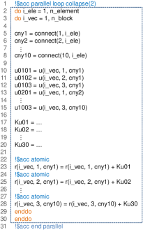
Next we port each kernel by using the loop directives with suitable options. Figure 1 shows a porting example of the EBE kernel with multiple vectors in Fortran. Each of the kernels in the solver has a nested loop with an inner loop length of 16. The length of the inner loop is not large; thus, we collapse these nested loops by adding collapse options in the loop directives. In the current specification of OpenACC, target loops must be adjacent to each other for collapsing loops. Thus, parts of the kernel must be computed redundantly (e.g., the node connectivity array is read redundantly in Fig. 1); however, collapsing of the loops enables coalesced memory accesses for the vectors leading to higher computing performance. In GPU computation, SIMT computation is applied automatically; thus we do not have to designate parallel code explicitly as in SIMD computation in CPUs. We insert atomic directives for adding thread-wise temporal variables to the resulting vector. Our previous study has shown that atomic operations attain higher performance than reordering the elements to avoid a data race using the coloring method [13], because atomic operations can retain data locality of nodal data (i.e., u and nodal coordinate information) and thus utilize the L2 cache more efficiently.

Figure 1: EBE kernel for multiple vectors on GPUs.

Figure 2: Vector inner product kernel for multiple vectors on GPUs.

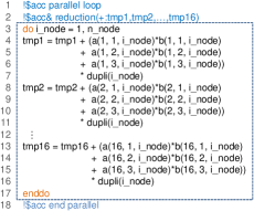
Although other calculations, such as multiplication, addition, and subtraction of vectors, can also be computed on GPUs by adding loop directives, we must take care when porting the inner product kernel with multiple vectors. In the case of inner vector products with a single vector, we can directly port the CPU code by inserting the reduction option in loop directives. However, the reduction option in OpenACC is available for scalars but not for arrays. Thus, the innermost loop cannot be parallelized directly in the present specification of OpenACC. Thereby, we allocate scalars corresponding to each of the multiple vectors and compute the reduction of these scalars in a single loop (Fig. 2). In this case, memory access becomes strided, possibly leading to performance decrease when compared with the single vector type inner product kernel. Adding collapse options with reduction options for arrays in OpenACC that enable contiguous memory access might be beneficial in this case.

Examining the parameters in OpenACC defining parallelism of computation is important for exhibiting high performance. In OpenACC, three hierarchies of gang, worker and vector determine the granularity of parallelization. The parameter gang corresponds to a thread block in an NVIDIA GPU, and vector corresponds to a thread. For instance, in EBE kernels, we must assign one thread per element to attain their optimal performances on GPUs. Without any instructions, threads can be unintendedly mapped; thus these two options, gang and vector, must be inserted in appropriate places explicitly. The length of vector, which corresponds to the block size in NVIDIA GPUs, is automatically determined by the compiler. In most cases, these parameters have little impact on performance; however, we searched for optimal parameters for core kernels in the solver to attain optimal performance. For EBE kernels, in which the usage of registers rather than the block size has the largest impact on the number of working threads, we can set their lengths of vector to 32. This saves the need for synchronization in the block among different warps; thus this parameter is expected to be the most optimal one.

4 Performance Measurements

In this section, we show the effectiveness of the developed solver through performance measurements.

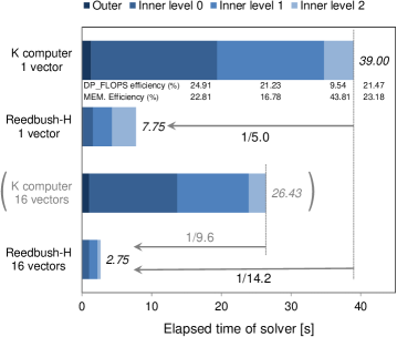
We first compare the performance of the ported solver on NVIDIA P100 GPUs with that of the base solver on the K computer. Here we use Reedbush-H of the Information Technology Center, The University of Tokyo for a computation environment with P100 GPUs [14]. The K computer is a massively parallel CPU-based supercomputer system at the Advanced Institute of Computational Science, RIKEN. The computation environments are summarized in Table 1. We continue to compute until the residual error in outer loop goes below $10^{-8}$. The maximum iteration and tolerance thresholds for inner loops greatly affect the convergence of the outer loop and whole computation time. In this paper, these parameters are empirically configured as in Table 2 so that the computation time for the whole solver is reduced. For performance measurement, we use a finite-element model with 125,177,217 degrees of freedom and 30,720,000 second-order tetrahedral elements. The material properties of the two-layered model are shown in Table 3. The computation time in the conjugate gradient loop is shown in Fig. 3. From the figure, we can see that the base solver attains 21.5% of peak FLOPS on the K computer system, which is very high performance for a low-order finite-element solver. Compared to this highly tuned CPU solver implementation, we confirmed that direct porting of the original solver without algorithm changes enabled 5.0 times speedup. By using the proposed method solving 16 vectors simultaneously in GPUs, the solver was accelerated further by 2.82 times per vector from the directly ported solver. This leads to 14.2 times speedup with respect to the base solver on the K computer. For comparison, we measured the computation time using 16 vectors on the K computer. As shown in Fig. 3, we attained 1.48 times speedup with regard to the original solver using single vector. Considering the speedup ratio is 2.82 between using 16 vectors and single vector on Reedbush-H, we can confirm that we have attained higher performance in P100 GPUs by introduction of dense computation, which is more effective for GPU computation. The speedup ratio in using 16 vectors is 9.6 between Reedbush-H and K computer. In standard finite-element solvers using sparse matrix storage formats, the expected speedup will be near the peak memory bandwidth ratio, which is 11.4 times in this case. However, for practical cases, the computation includes random accesses that severely degrade GPU performance; thus the speedup ratio is assumed to get much less than the peak bandwidth ratio. Thus, we can see that the 9.6 times speedup attained is reasonable performance. This speedup ratio is mainly due to the introduction of EBE multiplication, which has changed global memory bandwidth bound computation into cache memory bandwidth bound. We examine the cause of the performance improvement by checking the speedup of each kernel in Table 4. As the sparse matrix-vector product in inner loop level 2 is bound by reading the global matrix from memory, the total computation time is nearly constant regardless of the number of vectors multiplied. Thus, the efficiency of computation is significantly improved when 16 vectors are multiplied simultaneously. The reduction in random memory access in EBE kernels leads to performance improvement by 1.6–1.7 times. Although the performance of the inner vector product kernel decreased as a result of strided memory access, the acceleration of sparse matrix-vector products and EBE computation has a profound effect leading to performance improvement of the entire solver.

Table 1: Comparison of hardware capabilities of K computer and Reedbush-H.

	K computer	Reedbush-H (Tesla P100)
# of nodes	20	10
CPU/node	1 $\times$ eight-core	2 $\times$ eighteen-core
	SPARC64 VIIIfx	Intel Xeon E5-2695 v4
Accelerator/node	-	2 $\times$ NVIDIA P100
# of MPI processes/node	1	2
hardware peak DP	128 GFLOPS	5.30 TFLOPS (GPU only)
FLOPS /process
Bandwidth/process	64 GB/s	732 GB/s (GPU only)
Interconnect	Tofu (4 lanes $\times$	PCIe Gen3 $\times$ 16
	5GB/s in both directions)	+ NVLink (20 GB/s) $\times$ 2
		+ InfiniBand FDR 4 $\times$ 2
Compiler	Fujitsu Fortran	PGI compiler 17.5
	Driver Version 1.2.0
Compiler option	-Kfast,openmp,parallel,ocl	-ta=tesla:cc60,loadcache:L1
		-acc -Mipa=fast -fastsse -O3
MPI	custom MPI	OpenMPI 1.10.7

Table 2: Error tolerance $\overline{\epsilon}_{0-2}$ and maximum iteration $N_{0-2}$ used for our solver for solving measurement models and application problems.

Inner loop	Error tolerance	Maximum iteration
level 0	0.1	30
level 1	0.05	300
level 2	0.025	3,000

Table 3: Material properties of performance measurement models. $V_{p}$, $V_{s}$, and $\rho$ indicate primary wave velocity, secondary wave velocity, and density, respectively.

Layer	$V_{p}$ (m/s)	$V_{s}$ (m/s)	$\rho$ (kg/m3)
1	1,600	400	1,850
2	5,800	3,000	2,700

Figure 3: Performance comparison of the entire solver. Here, the computation time when using 16 vectors is divided by 16 and converted per vector.

Table 4: Performance of main kernels in Reedbush-H.

Kernel	Elapsed time per vector (s)		Speedup
	1 vector	16 vectors
SpMV ($\overline{\bf A}_{2}\overline{\bf u}_{2}$)	1.465	0.091	16.10
2nd order EBE (${\bf K}{\bf u}$)	0.044	0.025	1.78
2nd order EBE ($\overline{\bf K}\overline{\bf u}$)	0.687	0.401	1.71
1st order EBE ($\overline{\bf K}_{1}\overline{\bf u}_{1}$)	0.948	0.584	1.62
Inner product ($\overline{\bf p}\cdot\overline{\bf q}$)	0.213	0.522	0.41
Total time of the solver	7.75	2.75	2.82

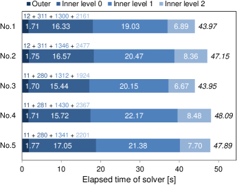
We next check the parallelization efficiency by measuring weak scaling. Here, we measure the elapsed time of the solver using the full Reedbush-H system with 240 P100 GPUs. The number of GPUs, degrees of freedom, and the number of elements of the models are shown in Table 5. Here, model No.1 is the same model as used in the performance comparison with the K computer. To assure that the convergence characteristics of the models are similar, we compared the number of iterations required for convergence of a standard conjugate gradient solver with a 3 $\times$ 3 block Jacobi preconditioner (from here on referred to as PCGE). PCGE corresponds to Algorithm 1(a) without the adaptive conjugate gradient preconditioner part (lines 8–17). From Table 5, we can see that the number of iterations in PCGE is nearly constant, and thus this model set is suitable for measuring weak scaling. Figure 4 shows the elapsed time of the developed solver and the total number of iterations required for convergence. Although there are slight fluctuations in the number of iterations of the inner loops, the computation time is roughly constant up to the full system.

Table 5: Model configuration for weak scaling in Reedbush-H.

Model	# of GPUs	Degrees of freedom (DOF)	DOF per GPU	# of elements	PCGE iterations
No.1	20	125,177,217	6,258,861	30,720,000	4,928
No.2	40	249,640,977	6,241,024	61,440,000	4,943
No.3	80	496,736,817	6,209,210	122,880,000	4,901
No.4	160	992,038,737	6,200,242	245,760,000	4,905
No.5	240	1,484,953,857	6,187,308	368,640,000	4,877

Figure 4: Performance in weak scaling. The numbers of iterations for the outer loop, inner loop level 0, inner loop level 1, and inner loop level 2 are written in the insets.

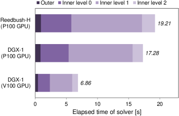
Finally, we check the effectiveness of the developed solver on the latest Volta GPU architecture. Here, we compare performance of four Reedbush-H nodes with eight P100 GPUs, a DGX-1 with eight P100 GPUs, and a DGX-1 with eight V100 GPUs [15] (Table 6). The target model size is 38,617,017 degrees of freedom and 9,440,240 tetrahedral elements, almost filling the 16 GB device memory of the eight P100 and V100 GPUs on each system. From Fig. 5, we can see that the elapsed time has decreased from 19.2 s to 17.3 s when DGX-1 (P100) is used. This performance difference may be attributed to the inter-node InfiniBand communication between the four Reedbush-H nodes in contrast to the intra-node communication inside a single DGX-1. In the comparison of the P100 and V100 versions of DGX-1, the elapsed time has decreased from 17.3 s to 6.86 s. This corresponds to 2.52 times speedup, higher than the 1.23 times increase in hardware peak memory bandwidth. Architectural improvements for caches contribute to this speedup ratio. Volta GPU has 128 kB of combined L1 cache/shared memory per SM and 6 MB of L2 cache per GPU, which are 5.3 times and 1.5 times larger than L1 and L2 cache of Pascal GPU, respectively. In the solver, random memory accesses in sparse matrix-vector multiplications is one of bottlenecks. Larger cache size in V100 GPU is thought to reduce memory bandwidth demand and improve performance of these kernels, including atomic addition part. Thereby it is inferred that these improvements in the hardware result in a speedup ratio more than the peak memory bandwidth ratio or the double-precision peak performance ratio.

Table 6: Comparison of hardware capabilities of Reedbush-H, P100 DGX-1, and V100 DGX-1. Latest compilers available in each environment are used.

	Reedbush-H (P100)	DGX-1 (P100)	DGX-1 (V100)
# of nodes	4	1	1
CPU/node	2 $\times$ eighteen-core	2 $\times$ twenty-core	2 $\times$ twenty-core
	Intel Xeon E5-2695 v4	Intel Xeon E5-2698 v4	Intel Xeon E5-2698 v4
Accelerators/node	2 $\times$ NVIDIA P100	8 $\times$ NVIDIA P100	8 $\times$ NVIDIA V100
MPI processes/node	2	8	8
GPU memory	16 GB	16 GB	16 GB
size/process
GPU peak DP	5.3 TFLOPS	5.3 TFLOPS	7.5 TFLOPS
FLOPS/process
GPU memory	732 GB/s	732 GB/s	900 GB/s
bandwidth/process
Interconnect	InfiniBand FDR 4 $\times$ 2	InfiniBand EDR $\times$ 4	InfiniBand EDR $\times$ 4
	+ PCIe Gen3 $\times$ 16	+ NVLink	+ NVLink
	+ NVLink
Compiler	PGI compiler 17.5	PGI compiler 17.9	PGI compiler 17.9
Compiler option	-ta=tesla:cc60	-ta=tesla:cc60	-ta=tesla:cc70
	-ta=loadcache:L1	-ta=loadcache:L1	-ta=loadcache:L1
	-acc -Mipa=fast	-acc -Mipa=fast	-acc -Mipa=fast
	-fastsse -O3	-fastsse -O3	-fastsse -O3
MPI	OpenMPI 1.10.7	OpenMPI 1.10.7	OpenMPI 1.10.7

Figure 5: Performance comparison of the entire solver on Reedbush-H, DGX-1 (P100), and DGX-1 (V100).

5 Application Example

In this section, we demonstrate the use of the developed solver by estimating the coseismic fault slip distribution in the 2011 Tohoku-oki earthquake. This estimation is important for considering earthquake generation processes. Previous studies [16], [17] have shown that approximation in the geometry of the crust significantly changes the slip distribution. Thus, conducting crustal deformation analysis reflecting local geometry is required.

First, we describe the method used to estimate the coseismic fault slip distribution following a previous study [18]. The assumed fault plane is divided into $n$ small unit faults, and the fault slip is expanded using these unit faults as bases:

$${\bf x}=\sum_{i=1}^{n}a_{i}\phi_{i},$$ (4)

where ${\bf x}$ is the fault slip distribution vector, $a_{i}$ is the coefficient for the $i^{th}$ unit fault slip, and $\phi_{i}$ is the distribution vector of the $i^{th}$ unit fault slip. We assume that observation data are available on the crustal surface at $m$ points, and that the coseismic crustal deformation can be regarded as a linear elastic deformation. Using Green’s function $g_{ji}$ (i.e., surface response on observation point $j$ for unit fault slip $\phi_{i}$), yields the following estimation of the slip distribution:

$$\left(\begin{array}[]{c}{\bf G}\\ \alpha{\bf L}\\ \end{array}\right){\bf a}=\left(\begin{array}[]{c}{\bf d}\\ {\bf 0}\\ \end{array}\right),$$ (5)

where ${\bf G}$ is an $m\times n$ matrix with components $g_{ji}$, and ${\bf d}$ is an $m$ dimensional vector of crustal deformation data on observation point $j$. ${\bf L}$ is a smoothing matrix introduced because ${\bf G}$ is generally ill-posed. $\alpha$ is a weighting factor defined using the L-curve method [19]. These Green’s functions are obtained by computing surface responses against $n$ unit fault slips. In typical problems, $n$ is of the order 10²–10³; thus, we must conduct crustal deformation computation more than 10² times. When we use finite-element models with 10⁸ degrees of freedom required for reflecting the geometry of the crust, this simulation leads to huge computational cost. In this analysis, multiple crustal deformation computations are performed for the same finite-element model; thereby, use of the developed solver is expected to lead to high speedup.

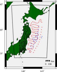
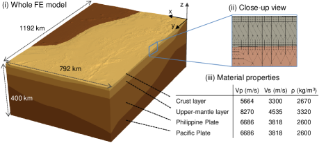
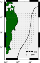
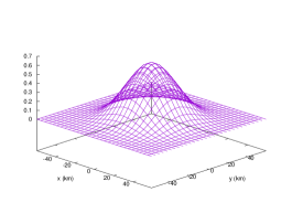
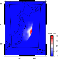
The four-layered 792 km $\times$ 1,192 km $\times$ 400 km target area is shown in Fig. 6. Modeling this area with a resolution of 1,000 m leads to a finite-element model consisting of 409,649,580 degrees of freedom and 100,494,786 tetrahedral elements (Fig. 7). We use the $x$, $y$, and $z$ components of GEONET, the $x$ and $y$ components of GPS-A, and the $z$ component of S-net for the observed crust-deformation data. The locations of the 184 input unit fault slips are shown in Fig. 9. For each point, Green’s functions with unit B-spline function fault slips (Fig. 9) are computed in the dip and strike directions. Thus, the total number of Green’s functions becomes $n$ = 184 $\times$ 2 = 368. We used 32 nodes of Reedbush-H and obtained 368 Green’s functions by conducting 23 sets of crustal deformation computations with 16 vectors. Figure 10 shows the estimated slip distribution obtained by solving Eq. (5) using the computed Green’s functions and observed data, a result consistent with previous studies [18].

Figure 6: Target region of the application example (black line). The black, blue, and red points indicate the positions for GEONET, GPS-A, and S-net, respectively.

Figure 7: Finite-element model used for the application example.

Figure 8: Location of the centers of the unit fault slips.

Figure 9: Distribution of unit fault slip.

Figure 10: Estimated coseismic slip distribution.

The computation time for solving systems of linear equations was 828 s for 368 crustal deformation computations. This computation is 29.2 times better in performance (5.11 times larger problem $\times$ solved 5.71 times faster) than previous studies on smaller computational environments in [13] with eight K40 GPUs, which conducted 360 crustal deformation computations with 80 million degrees of freedom in 4,731 s. From here we can see that the developed solver enabled reduction in computation time for a practical problem. In the future, we plan to use this method to optimize the crustal structure based on 10⁶ cases of Monte Carlo crustal deformation computations with varying geometries and material properties.

6 Concluding Remarks

In this paper, we accelerated a low-order unstructured 3D finite-element solver targeting multiple large-scale crustal deformation analyses. When we introduce accelerators, it is important to redesign the algorithm as its computer architecture greatly changes. Based on a CPU-based solver attaining high performance on the K computer, we developed the solver algorithm more appropriate for a GPU architecture and then ported the code using OpenACC. Here, we changed the algorithm such that multiple cases of finite-element simulations are conducted simultaneously thereby reducing random access and memory transfer per simulation case. When the runtime on 20 K computer nodes and ten Reedbush-H nodes (20 P100 GPUs) were compared, the directly ported solver attained 5.0 times speedup, and the ported solver with modification to the algorithm attained 14.2 times speedup. We confirm that this modification is important to exhibit high performance in P100 GPUs and more effective for GPU-based Reedbush-H than for CPU-based K computer. The developed solver is also highly effective on the Volta GPU architecture; we confirmed 2.52 times speedup with respect to eight P100 GPUs to eight V100 GPUs. This acceleration enabled 368 crustal deformation computations targeting northeast Japan with 400 million degrees of freedom in 828 s on 32 Reedbush-H nodes, which is significantly faster than in the previous study. The entire procedure of algorithm modification and OpenACC directive insertion was completed within two weeks; hence, we can see that high-performance gain can be attained with low development cost by using a suitable porting strategy. Fast computations realized by the developed method are expected to be useful for quality assurance of earthquake simulations in the future.

References

- [1] H. Miyazaki, Y. Kusano, N. Shinjou, F. Shoji, M. Yokokawa, and T. Watanabe. Overview of the k computer system. FUJITSU Sci. Tech. J., 48(3):302–309, 2012.
- [2] T. Ichimura, K. Fujita, S. Tanaka, M. Hori, L. Maddegedara, Y. Shizawa, and H. Kobayashi. Physics-based urban earthquake simulation enhanced by 10.7 blndof x 30 k time-step unstructured fe non-linear seismic wave simulation. Proceedings of the International Conference on High Performance Computing, Networking, Storage and Analysis, pages 15–26, 2014.
- [3] T. Ichimura, K. Fujita, P. E. B. Quinay, L. Maddegedara, M. Hori, S. Tanaka, Y. Shizawa, H. Kobayashi, and K. Minami. Implicit nonlinear wave simulation with 1.08t dof and 0.270t unstructured finite elements to enhance comprehensive earthquake simulation. Proceedings of the International Conference on High Performance Computing, Networking, Storage and Analysis, pages 1–12, 2015.
- [4] OpenACC. http://www.openacc.org.
- [5] K. Fujita, T. Yamaguchi, T. Ichimura, M. Hori, and L. Maddegedara. Acceleration of element-by-element kernel in unstructured implicit low-order finite-element earthquake simulation using openacc on pascal gpus. Proceedings of the Third International Workshop on Accelerator Programming Using Directives, pages 1–12, 2016.
- [6] K. Fujita, T. Ichimura, K. Koyama, H. Inoue, M. Hori, and L. Maddegedara. Fast and scalable low-order implicit unstructured finite-element solver for earth’s crust deformation problem. Proceedings of the Platform for Advanced Scientific Computing Conference, pages 11–20, 2017.
- [7] NVIDIA Pascal GPU. http://www.nvidia.com/object/tesla-p100.html.
- [8] NVIDIA Volta GPU. http://www.nvidia.com/en-us/data-center/tesla-v100.
- [9] HJ Melosh and A Raefsky. A simple and efficient method for introducing faults into finite element computations. Bulletin of the Seismological Society of America, 71(5):1391–1400, 1981.
- [10] G. H. Golub and Q. Ye. Inexact conjugate gradient method with inner-outer iteration. SIAM., Journal on Scientific Computing, 21(4):1305–1320, 1997.
- [11] A. Brandt. Multi-level adaptive solutions to boundary-value problems. Mathematics of computation, 31(138):333–390, 1977.
- [12] J. M. Winget and T. J. R. Hughes. Solution algorithms for nonlinear transient heat conduction analysis employing element-by-element iterative strategies. Computer Methods in Applied Mechanics and Engineering, 52:711–815, 1985.
- [13] K. Fujita, T. Yamaguchi, T. Ichimura, M. Hori, and L. Maddegedara. Acceleration of element-by-element kernel in unstructured implicit low-order finite-element earthquake simulation using openacc on pascal gpus. Third Workshop on Accelerator Programming Using Directives, pages 1–12, 2016.
- [14] Reedbush-H. http://www.cc.u-tokyo.ac.jp/system/reedbush/Reedbush-EN.pdf.
- [15] NVIDIA DGX-1. http://www.nvidia.com/dgx1.
- [16] T. Masterlark. Finite element model predictions of static deformation from dislocation sources in a subduction zone: Sensitivities to homogeneous, isotropic, poisson-solid, and half-space assumptions. Journal of Geophysical Research, 108(B11):2540, 2003.
- [17] K. L. Hughes, T. Masterlark, and W. D. Mooney. Poroelastic stress-triggering of the 2005 m8.7 nias earthquake by the 2004 m9.2 sumatra-andaman earthquake. Earth planet. Sci. Lett., 293:289–299, 2010.
- [18] R. Agata, T. Ichimura, K. Hirahara, M. Hyodo, T. Hori, and M. Hori. Robust and portable capacity computing method for many finite element analyses of a high-fidelity crustal structure model aimed for coseismic slip estimation. Computers & Geosciences, 94:121–130, 2016.
- [19] P. C. Hansen. Analysis of discrete ill-posed problems by means of the l-curve. SIAM review, 34(4):561–580, 1992.