Normal behaviour models for wind turbine vibrations: An alternative approach

Abstract

To monitor wind turbine vibrations, normal behaviour models are built to predict tower top accelerations and drive-train vibrations. Signal deviations from model prediction are labelled as anomalies and are further investigated. In this paper we assess a stochastic approach to reconstruct the $1$ Hz tower top acceleration signal, which was measured in a wind turbine located at the wind farm Alpha Ventus in the German North Sea. We compare the resulting data reconstruction with that of a model based on a neural network, which has been previously reported as a data-mining algorithm suitable for reconstructing this signal. Our results present evidence that the stochastic approach outperforms the neural network in the high frequency domain ($1$ Hz). Although neural network retrieve accurate step-forward predictions, with low mean square errors, the stochastic approach predictions better preserve the statistics and the frequency components of the original signal, remaining high accuracy levels. The implementation of our stochastic approach is available as open source code and can easily be adapted for other situations involving stochastic data reconstruction. Based on our findings we argue that such an approach could be implemented in signal reconstruction for monitoring purposes or for abnormal behaviour detection.

1 Introduction

As the number of wind turbines installed worldwide increases, the reduction of operational and maintenance cost by enhanced surveillance gains on importance [1]. Recent reviews on condition monitoring of wind turbines [2, 3, 4], recognize the importance that a reliability based maintenance system has on reducing the cost of energy. Although it is possible to monitor wind turbine functioning with 10-minute average SCADA data, part of the information is lost when data is averaged; a mixed system, combining SCADA data and conventional high frequency sensors is expected in the future [3].

Zaher et al [5] described the lack of failure records as the main challenge for early failure detection, which emphasizes the importance of normal behaviour modelling. Such models are built empirically, i.e. using only measured signals, and refer to the expected value the signal should have based on its own historical records. An anomaly in the signal is detected when the error on its prediction, made by the normal behaviour model, increases over several subsequent values.

Previous investigations have built normal behaviour models with data-mining algorithms on SCADA data. Most of them are based on $10$-minute data [6]. Cruz Garcia and co-workers [7] presented their application to detect anomalies in wind turbine gearboxes. In Ref. [5] the authors proposed a framework for their combination into a single user interface to facilitate their use, while Ref. [8] shows that a normal behaviour model based on neural networks (NN) outperforms a regression based one. But some scientists also evaluate data with higher sampling frequency, Kusiak and co-workers [9] analysed the performance of various NN algorithms to detect bearing faults on wind turbines. In Refs. [10] and [11], they evaluated wind turbine vibrations in time domain with $10$-second sampling signals from drive-train vibrations and tower top accelerations.

In contrast to existing methods, signals can also be reconstructed based on a stochastic approach, which has not been assessed so far for the creation of normal behaviour models. In a previous work [12], we demonstrated its value to estimate fatigue loads for wind turbines based on reconstructed signals. Moreover, this stochastic approach was already combined with NN models [13] for improving forecast of air quality. The objective in this paper is to assess the stochastic approach as basis for normal behaviour models. We evaluate the performance of such model to monitor vibrations on wind turbines and compare it versus one based on a NN, which was found the most suitable NN model to reconstruct the tower top acceleration [11]. We focus our assessment on the similarities and differences between both approaches, we then discuss our findings with respect to the limitations imposed by the specific case evaluated.

We start in Sec. 2 by describing in detail the data used in this investigation, obtained from one wind turbine in an offshore wind farm. In Sec. 3 both the NN model and our stochastic approach are introduced; then, the results obtained from them are properly plotted in the figures and tables below. In Sec. 4 we compare the results of both approaches when reconstructing one month of the tower acceleration measured at one turbine. Section 5 concludes the paper.

2 Data description

Wind turbine vibrations can easily be assessed monitoring two standard operational signals: drive-train and tower top acceleration [11]. In this paper, we limited the analysis to the second one to assess the reconstruction of signals with both the neural network model and the stochastic approach.

The data analysed in this paper correspond to measurements carried out in one 5MW Senvion wind turbine AV-04 of the offshore wind farm Alpha Ventus [14]. Alpha Ventus is the first offshore wind farm in Germany, located at Borkum West in the North Sea, $54.3^{o}$N-$6.5^{o}$W.

The turbine is sujected most of the time to undisturbed inflow due to its position in the first row of turbines, located at the western past of the wind farm. The support structure of the turbine combines a rather stiff and hydrodynamically transparent jacket structure with a tubular tower on top. In such a design the tower top acceleration signal is dominated by the dynamic response on aerodynamic excitation mainly at the first bending natural frequency of the system and at multiples of the blade passing frequency. Wave excitation plays only a minor role.

Data include all wind speed and tower top acceleration values recorded in October and November 2014, regardless of the operational and wind flow conditions. Therefore, $29$ days were available in October ($2555805$ values) and $21$ days in November ($1859179$ values). We only removed incorrect measurements from the data collected, either because they were identified by the recording system with a flag (’99999’ in our case) or because their values were out of reasonable physical values, namely $x>\bar{x}+5\sigma$. Wind speed and tower acceleration values were available with sampling ratios of $1$ Hz and $50$ Hz respectively, thus the last one was down-sampled to $1$ Hz in order to complete the analysis.

Wind speeds were measured by a cup anemometer included in the meteorological station located on top of the nacelle. Tower top longitudinal accelerations were recorded by an accelerometer positioned at the bottom of the nacelle, near its connection to the upper part of the tower. Figure 1 illustrates the characteristics of the data in time and frequency domain.

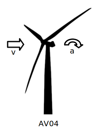
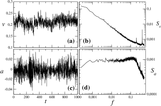
Figure 1: Examples of (a-b) wind speed and (c-d) tower acceleration signals in Alpha Ventus wind farm. In the left one ilustrates the time-domain of both quantities while in the right the frequency domain is shown for the full datasets of October 2014. All data was normalized to fulfill all confidentiality protocols (see text). Frequency units are Hertz and time is given in seconds. Both wind velocity and tower acceleration are normalized to maximal observed values.

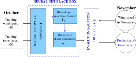
Figure 2: Schematic illustration of the neural network (NN) approach, indicating the development and test of neural networks for signal reconstruction. Here the particular case of tower acceleration reconstruction is given.

To protect sensitive manufacturer information we normalized the values. Wind speeds recorded included the whole operational range of the wind turbine. Furthermore, we divided measurements in two sets according to different purposes: data collected in October were used to estimate the parameters in each model, while data collected in November were used to test each model performance.

3 Methods and results

Each approach to construct a normal behaviour model is introduced in a concise manner. Where convenient, we provide references to literature with extensive details about neural networks and the stochastic approach. At the end of the section, we describe the performance metrics utilised for the assessment.

Zhang and Kusiak [11] evaluated a pool of potential input variables to predict tower top acceleration signal with a wrapper algorithm [15], which includes the predictor model to search for the variables that reduce prediction error (a posteriori approach). They found wind speed, tower acceleration and wind direction relevant. Since our evaluation focused on the approaches themselves, we limited the pool of potential input variables to a single external signal (wind speed) and previous values of the tower top acceleration to have the same number of inputs for each approach.

3.1 Neural networks: a deterministic approach

Neural networks transform input variables with a linear coefficient and a non-linear function. This is repeated, in a chain, over a variable number of layers, where each output layer becomes the input of the next one. The output of the last layer is the final prediction made for the target value. In this analysis, we utilised a non-linear auto-regressive with exogenous inputs (NARX) neural network, which is a recurrent network, i.e. it includes one or more feedback loops. Thus, the approach followed to estimate the predicted value of the tower top acceleration, given by

$$\hat{a}(t)=f[a(t-\Delta t),\dots,a(t-n_{a}\Delta t),v(t-\Delta t),\dots,v(t-n_{v}\Delta t)]+e(t),$$ (1)

involves the use of its $n_{a}$ previous values ($a(t-\Delta t),\cdots,a(t-n_{a}\Delta t)$) and those of the $n_{v}$ previous wind speeds ($v(t-\Delta t),\cdots,v(t-n_{v}\Delta t)$) through a smooth unknown function $f()$. An extra random component $e(t)$ represents a random error, which has a zero mean and is independent of $v$ and $a$ [16]. The time-dependent predicting function $\hat{a}(t)$ can be taken as an evolution equation.

To create the baseline normal behaviour model we used a NN to approximate $f()$, which is a recursive non-linear transformation of its inputs. Zhang and Kusiak [11] demonstrated that NNs were the most suitable algorithm to create a normal behaviour model for the tower top acceleration of a wind turbine when compared with neural network ensemble, boosting regression trees, support vector machine, random forest with regression, standard classification and regression tree and K-nearest neighbour. In our investigation, we used a NN with two layers (two transformations). The first one (hidden layer) consisted of $n_{h}$ neurons, which apply non-linear transformations via a sigmoid function; the second one (output layer) was formed by a single neuron, which performed an extra linear transformation, with given weights $w_{i}$.

To optimize the neural network we can also include a finite number of feedback loops for previous values of the tower top accelerations ($a,n_{a}$) and wind speeds ($v,n_{v}$), thus we have three parameters to determine ($n_{h},n_{v},n_{a}$).

First, we divided data from October 2014 using the hold out method [15] in sub-sets for model training (70%), validation (20%) and test (10%). Then, we selected the number of neurons in the hidden layer ($n_{h}$), the number $n_{v}$ of input delays for the wind speed $v$ and the number $n_{a}$ of output delays for the tower top acceleration $a$ with a wrapper algorithm [17], which searched for optimum prediction in the ranges $n_{h},n_{a},n_{v}\in\{1,\cdots,50\}$.

The optimization of the unknown function $f$ was set to minimize mean squared error

$$\mathit{MSE}=\frac{1}{n}\sum_{i=1}^{n}(\hat{y}_{i}-y_{i})^{2},$$ (2)

using the Levenberg-Marquardt algorithm. As a result, the architecture of the NARX network consisted on $25$ neurons in the hidden layer ($n_{h}=25$), three input delays ($n_{v}=3$) and one output delay ($n_{a}=1$).

Figure 2 depicts the development and utilization of the NN model investigated. From left to right, first we used wind speeds and tower top accelerations collected in October 2014 to define the constitutive components of the model, which is named a neural net black box in Fig. 2. Once the evolution equation $\hat{a}(t)$ was defined, we used wind speeds collected in November 2014 to predict the tower top acceleration signal, as well as to evaluate the performance of the model.

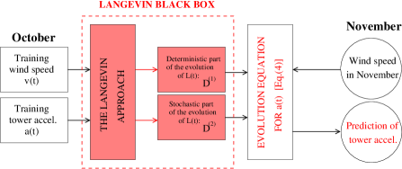
Figure 3: Schematic illustration of the Langevin (stochastic) approach. Here the particular case of tower acceleration reconstruction at Alpha Ventus is given.

3.2 Stochastic approach: the Langevin model

The Langevin model is a framework developed from the pioneering work by Peinke and Friedrich in 1997 [18, 19], which consists of a direct method for extracting the evolution equation of stochastic series of measurements. Several applications were proposed and developed, e.g. in turbulence modelling, in medical EEG monitoring and in stock markets. See Ref. [20] for a review. In the context of wind energy, this framework has shown the ability for predicting power curves of single wind turbines as well as of equivalent power curves for entire wind farms, and also to properly reproduce the increment statistics of power and torque in single wind turbines from wind speed measurements [21].

Figure 3 depicts the development and utilization of the stochastic approach investigated. Our stochastic framework, instead of computing non-linear functions and weights, which optimize a set of output compared to input data, retrieves two single functions of the variables involved. One of such functions, below symbolized by $D^{(1)}$, governs the deterministic contribution for the time variation of the output variable, while the other function, $D^{(2)}$, accounts for the stochastic fluctuations that include all the non-observable degrees of freedom present in the system. See the illustration in Fig. 4.

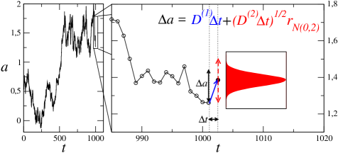
Figure 4: Illustration of the stochastic approach, while integrating the evolution equation (4), composed by its two contributions, the deterministic contribution $D^{(1)}$ which governes the tendency of the evolving observable (blue), and the stochastic fluctuations accounted by $D^{(2)}$ (red) added to the deterministic part.

Having wind speeds $v(t)$ and tower accelerations $a(t)$, the following evolution equation for the later quantity is used:

$$\frac{da}{dt}=D^{(1)}(a,v)+\sqrt{D^{(2)}(a,v)}\Gamma_{t},$$ (3)

with $\Gamma_{t}$ representing a Gaussian $\delta$-correlated white noise, i.e. $\langle\Gamma_{t}\rangle=0$ and $\langle\Gamma_{t}\Gamma_{t^{\prime}}\rangle=2\delta(t-t^{\prime})$.

The reconstruction of the tower acceleration $a(t)$ follows therefore directly from the stochastic integration of Eq. (3) which yields:

$$a(t+\Delta t)=a(t)+D^{(1)}(a,v)\Delta t+\sqrt{D^{(2)}(a,v)\Delta t}\;r_{N(0,2)},$$ (4)

where $r_{N(0,2)}$ is a random number from a Gaussian distribution with zero mean and variance equal to two. Details are illustrated in Fig. 4 and can be found in Ref. [20].

Function $D^{(1)}$ is also called drift function, while function $D^{(2)}$ is typically named as the diffusion function. Since the drift and diffusion functions have a physical interpretation, one could apply the model in Eq. (3) to a particular system and define ad hoc the functional shape of both functions from physical reasoning. Next we explain how to compute these both functions.

The derivation is performed through the computation of the corresponding first and second conditional moments [12], respectively

$$M^{(1)}_{v^{\ast}}(a,\tau) = \left\langle a(t+\tau)-a(t)\right\rangle|_{a(t)=a,v(t)=v^{\ast}},$$ (5a)

$$M^{(2)}_{v^{\ast}}(a,\tau) = \left\langle(a(t+\tau)-a(t))^{2}\right\rangle|_{a(t)=a,v(t)=v^{\ast}}.$$ (5b)

where $\langle\cdot\rangle|_{X(t)=x}$ indicates the average over the full time series, whenever $X(t)$ takes the value $x$, defined within an interval.

Figure 5a shows the first conditional moment for different values of the tower acceleration. Since it can be shown that drift ($D^{(1)}$) and diffusion functions ($D^{(2)}$) in Eq. (3) are, apart from a multiplicative constant ($1/k!$), the derivative with respect to the time-gap $\tau$ of the first and second conditional moments respectively, we can define both functions directly from the conditional moments, namely:

$$D^{(k)}(a,v)=\lim_{\tau\rightarrow 0}\frac{1}{k!}\frac{M_{v}^{(k)}(a,\tau)}{\tau}.$$ (6)

In other words, by taking the slope of the linear regression for each conditional moment one arrives to the corresponding value of function $D^{(1)}$ and $D^{(2)}$. Indeed, as sketched in Fig. 5a, within a sufficiently low range of $\tau$ values, here three time-steps of the set of measurements, the conditional moments $M^{(1)}$ and $M^{(2)}$ depend linearly on $\tau$. Figures 5b and 5c show both drift and diffusion functions, ($D^{(1)}$) and ($D^{(2)}$) respectively, for a range of $a$-values at different velocities. Notice that while the diffusion function shows a quadratic dependence on the tower acceleration, the drift function exhibits a cubic dependence with a dominant linear term having one single fixed point at $a=0$ which corresponds to the equilibrium position of tower vibrations.

It is important to stress that our framework is based on the assumption that the observable follows a Markov process, which means nothing else than that the noise $\Gamma_{t}$ is $\delta$-correlated as mentioned above. Though, one advantage of this Langevin data reconstruction is that it also works in some cases where the Markov test fails [22]. The full implementation in one- and two-dimensions of this approach is already public available [23]. Improvements on the noise term are beyond this paper, but were already addressed previously[24, 25].

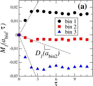
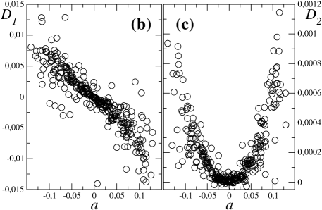
Figure 5: Illustration of (a) the first conditional moment for three different bin values of the tower acceleration as defined in Eqs. (5). Here $v^{\ast}$ is given by the average velocity found during October. Numerical result for (b) the drift $D^{(1)}(a,v)$ and (c) the diffusion $D^{(2)}(a,v)$ in the Langevin equation given by Eq. (6), plotted as function of $a$ alone, i.e. they are projected at the $a$-axis to emphasize the linear and quadratic dependency of $D^{(1)}$ and $D^{(2)}$ respectively for the largest range of acceleration values.

3.3 Performance evaluation

To compare both approaches, we consider the distribution of all values predicted from each model for November 2015, in particular their four first statistical moments, namely the mean, the standard deviation, the skewness and the kurtosis. Notice that, while mean and standard deviation are sufficient for characterizing the distribution of Gaussian processes, in general, higher-order moments should be checked for ascertaining if the process is non-Gaussian or not. The corresponding results are shown in Fig. 6 and Tab. 1.

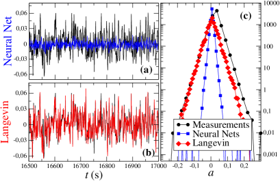
Figure 6: Sample of data series of tower acceleration from measurements at AV04 in Alpha Ventus and the acceleration reconstruction models using (a) NARX neural networks and (b) the Langevin model. In both cases, one also plots (black lines) the corresponding series of measurements for better comparison. The corresponding value distribution of these series is displayed in (c) with symbols for the full month of November 2014.

Additionally, to evaluate the prediction of both models we use four different metrics, namely the mean absolute error

$$\mathit{MAE}=\frac{1}{n}\sum_{i=1}^{n}|\hat{y}_{i}-y_{i}|,$$ (7)

the standard deviation of the absolute error

$$\mathit{SDofAE}=\sqrt{\frac{1}{n}\sum_{i=1}^{n}\left(|\hat{y}_{i}-y_{i}|-\frac{1}{n}\sum_{i=1}^{n}|\hat{y}_{i}-y_{i}|\right)^{2}},$$ (8)

the mean square error (already presented in Sec. 3, Eq. (2)) and the standard deviation of the square error

$$\mathit{SDofSE}=\sqrt{\frac{1}{n}\sum_{i=1}^{n}\left[(\hat{y}_{i}-y_{i})^{2}-\sum_{i=1}^{n}(\hat{y}_{i}-y_{i})^{2}\right]^{2}},$$ (9)

where $\hat{y}_{i}$ denotes the $i$th measured value of the property $y$, and $y_{i}$ the corresponding modelled value, either with NN or with the Langevin model.

Signal	Mean	Std. Dev.	Skewness	Kurtosis
Measurements	-2.07E-3	24.7E-3	11.6E-3	5.07
NN	-2.15E-3	7.39E-3	-30.1E-3	6.31
Langevin model	-1.71E-3	25.6E-3	-3.59E-3	2.37

Table 1: First four statistical moments of the value distributions shown in Fig. 6d for the normalised measurements and the reconstructed signals with each one of both models.

Signal	MAE	SDofAE	MSE	SDofSE
NN	0.031	0.032	2.0E-3	65.6E-3
Langevin model	0.027	0.031	1.6E-3	0.7E-3

Table 2: Performance of both models, using the metrics defined in Eqs. (2),(7)-(9), namely the mean of the absolute error, Eq. (7), its standard deviation, Eq. (8), the mean square error, Eq. (2) and its standard deviation, Eq. (9).

References [11] and [26] reported these metrics to select the best data-mining technique and to derive models for the normal behaviour of wind turbine vibration and to detect faults in wind turbine gearboxes. Moreover, they have been commonly used to evaluate the accuracy of models utilised for regression analysis in wind energy applications [9, 10, 11, 26]. The correspondig results comparing the NN and the stochastic approach are summarized in Tab. 2.

Finally, we also analyse the temporal correlations of the data. Therefore we use two methods, namely we calculate the power spectra and analyse the statistics of the temporal increments

$$\Delta a(t,\tau)=a(t+\tau)-a(t),$$ (10)

where $\tau=n\Delta t$ is an integer number $n$ of consecutive time-steps $\Delta t$. Note that the second moment of the increments $\Delta a$, given by $\langle(\Delta a)^{2}\rangle$, corresponds to the power spectrum. The power spectrum of the reconstructed signals are plotted in Fig. 7, showing how the frequency components are reconstructed. The statistics of the increments is given in Fig. 8, from which we will ascertain how good the model retrieves the evolution of the process throughout the succession of measurements [20].

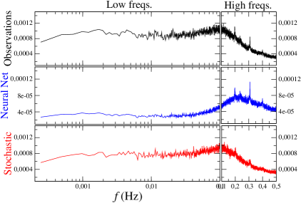
Figure 7: Spectrum of original signal (top) and the corresponding reconstructed signals, one using the neural network (middle) and the other using our proposed stochastic approach (bottom). Notice that the high frequency domain is plotted in a linear frequency scale, while the low frequency domain is plotted in the logarithmic scale.

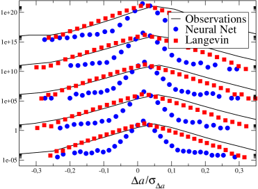
Figure 8: Two-point statistics of the tower acceleration (lines) and the corresponding reconstructed signals, i.e. value distributions of $\Delta a(t)=a(t+\tau)-a(t)$. From top to bottom one has $\tau=1,2,4,8$ and $16$ seconds. The vertical shift of the distribution is for better visualization.

4 Discussion: comparing both approaches

To evaluate the suitability of the stochastic approach, described above, for modelling normal behaviour of wind turbine vibrations, we compare it with the neural network [11].

Figures 6a and 6b show normalized samples of the original tower top acceleration and its two reconstructions. Already in these plots it is clear the stronger resemblance between the reconstructed data from the stochastic approach and the set of tower acceleration measurements. While the NN reconstruction keeps the average value of the tower oscillations, their range of amplitudes is not as well reproduced as with the stochastic approach.

This feature is more evident in the plot of Fig. 6c: both the stochastic and the NN models retrieve the approximate distribution of values of the original signal (symbols), but the full range of the tower acceleration values observed in measured distribution (bullets) is reproduced by the distribution obtained from the Langevin model (diamonds) but not from the NN model (squares).

Furthermore, the empirical distribution is clearly non-Gaussian, showing exponential tails. Table 1 compares the first four moments of all three distributions in Fig. 6c. While NN reproduces the mean more accurately, the standard deviation is much better modelled with the stochastic approach. In other words, while the average behaviour is better modelled with NN, for properly reproduced the amplitude of tower vibrations the stochastic approach is better suited.

Curiously however, while the (weak) skewness is also better approximated by the stochastic approach, the value of the kurtosis is better reproduced by the NN model.

The performance of both models was also assessed using the metrics introduced above, Eqs. (7)-(9) and results are given in Tab. 2: one clearly sees a tendency for lower values of $\mathit{MAE}$, $\mathit{SDofAE}$, $\mathit{MSE}$ and $\mathit{SDofSE}$. For such metrics, one concludes that the stochastic approach results have comparable accuracy or are even more accurate than the results from NN models, in what concerns the predictions for the tower top acceleration.

As for the temporal correlations of the signals, the results plotted in Fig. 7 show the spectral behaviour of the two models compared with the measurements of the tower acceleration. While NN better reproduces the periodic models (picks in the spectrum) present in the measurements, it is worse for the low-frequency range and for the overall amplitudes of the spectrum. Notice the different vertical scale used for plotting the NN results. The stochastic approach smooths out the periodic modes, but reproduces the overall shape of the empirical power spectrum.

Finally, a better reconstruction of two-point statistics is also obtained through the stochastic approach, as shown in Fig. 8. It is clear that the stochastic approach better reconstructs the differences $\Delta a$ between consecutive values in the tower acceleration series, only with some small deviations for the largest differences. This shows furthermore that the assumption of Markovian process with Langevin noise is considerably reliable for these data sets.

5 Conclusions

We have presented a stochastic approach which is capable of modelling the normal behaviour of wind turbine tower acceleration for its monitoring. Our results demonstrate that, compared to neural network (NN) models and using a single input, the Langevin model is able to better reconstruct non-Gaussian fluctuations of signals. In general both models provide a good estimate for the central part of the original signal, but the stochastic approach also reconstructs its complete variance.

We have also shown that a normal behaviour model based on the stochastic approach provides more information about the original signal than one based on NNs. Still, one should emphasize that previous publications on normal behaviour models, to monitor vibration of wind turbines based on SCADA [10, 11] using 10-second sampling signals, demonstrated the suitability of NNs and control charts as a method to monitor signals in time-domain. Our results for NN match the applications found in the literature, where they have been used with 10-minute sampling time-series [8]. When using low-frequency data, the NN is as good as our stochastic approach.

Putting our results in perspective, we state that NNs are a good choice to predict average values or low fluctuating signals. For situations where $10$-minute data is not sufficiently sampled, namely when dealing with cumulative loads for which the large wind fluctuations of short intervals play an important role. In these situations, since the stochastic approach depends on the conditional limit of the first two moments in the data, when the time-lag between measurements tends to zero, it is better suited for signals with a higher sampling rate.

All in all, in those cases where the sampling ratio is low, the NNs remain as a good option to take into account, as the monitoring is sufficient in time-domain and the requirements to apply the stochastic approach are not always fulfilled. In cases where the sampling ratio of the signal is high ($1$ Hz in our case), the stochastic approach is clearly a better choice. It allows for monitoring normal behaviour in time-domain as with NNs, but also extends the possibilities to the frequency-domain. To notice that a central advantage of the Langevin approach is that deterministic and noisy contributions can be separated leading to improvements in the statistics reproduction of the output fluctuations, since with the noisy contribution as a numerical function, quite general heavytailed distributions can be grasped. The study of the long time behavior of the deterministic part of the Langevin equation used in the stochastic approach can also provide information about the health of the structure, in a similar direction as previous work [27]. From this paper, one can now use the available routines [22, 23] and extend the stochastic approach here applied to other wind turbine properties, in particular to other loads.

References

References

- [1] W. Yang, P. J. Tavner, C. J. Crabtree, Y. Feng, Y. Qiu, Wind turbine condition monitoring: technical and commercial challenges, Wind Energy 17 (August 2012) (2014) 673–693. doi:10.1002/we.
- [2] A. Kusiak, Z. Zhang, A. Verma, Prediction, operations, and condition monitoring in wind energy, Energy 60 (2013) 1–12. doi:10.1016/j.energy.2013.07.051.
- [3] K.-S. Wang, V. S. Sharma, Z.-Y. Zhang, SCADA data based condition monitoring of wind turbines, Advanced Manufacturing 2 (March 2014) (2014) 61–69. doi:10.1007/s40436-014-0067-0.
- [4] P. Tchakoua, R. Wamkeue, M. Ouhrouche, F. Slaoui-Hasnaoui, T. Tameghe, G. Ekemb, Wind Turbine Condition Monitoring: State-of-the-Art Review, New Trends, and Future Challenges, Energies 7 (4) (2014) 2595–2630. doi:10.3390/en7042595.
- [5] A. Zaher, S. McArthur, D. Infield, Online wind turbine fault detection through automated SCADA data analysis, Wind Energy 12 (January 2009) (2009) 574–593. doi:10.1002/we.319.
- [6] J. Wang, J. Heng, L. Xiao, C. Wang, Research and application of a combined model based on multi-objective optimization for multi-step ahead wind speed forecasting, Energy 125 (2017) 591–613. doi:10.1016/j.energy.2017.02.150.
- [7] M. Cruz Garcia, M. A. Sanz-Bobi, J. del Pico, SIMAP: Intelligent System for Predictive Maintenance. Application to the health condition monitoring of a windturbine gearbox, Computers in Industry 57 (6) (2006) 552–568. doi:10.1016/j.compind.2006.02.011.
- [8] M. Schlechtingen, I. Ferreira Santos, Comparative analysis of neural network and regression based condition monitoring approaches for wind turbine fault detection, Mechanical Systems and Signal Processing 25 (5) (2011) 1849–1875. doi:10.1016/j.ymssp.2010.12.007.
- [9] A. Kusiak, A. Verma, Analyzing bearing faults in wind turbines: A data-mining approach, Renewable Energy 48 (2012) 110–116. doi:10.1016/j.renene.2012.04.020.
- [10] A. Kusiak, Z. Zhang, Analysis of Wind Turbine Vibrations Based on SCADA Data, Journal of Solar Energy Engineering 132 (3) (2010) 031008. doi:10.1115/1.4001461.
- [11] Z. Zhang, A. Kusiak, Monitoring Wind Turbine Vibration Based on SCADA Data, Journal of Solar Energy Engineering 134 (2) (2012) 021004. doi:10.1115/1.4005753.
- [12] P. G. Lind, I. Herráez, M. Wächter, J. Peinke, Fatigue Load Estimation through a Simple Stochastic Model, Energies 7 (12) (2014) 8279–8293. doi:10.3390/en7128279.
- [13] A. Russo, F. Raischel, P. G. Lind, Air quality prediction using optimal neural networks with stochastic variables, Atmospheric Environment 79 (2013) 822–830. doi:10.1016/j.atmosenv.2013.07.072.
- [14] K. Müller, P. W. Cheng, Validation of uncertainty in IEC damage calculations based on measurements from alpha ventus, Energy Procedia 94 (2016) 133–145. doi:10.1016/j.egypro.2016.09.208.
- [15] T. Borovicka, M. J. Jirina, P. Kordik, M. Jirina, Selecting representative data sets, in: A. Karahoca (Ed.), Advances in Data Mining Knowledge Discovery and Applications, 2012, pp. 43–70. doi:10.5772/3349.
- [16] T. Hastie, R. Tibshirani, J. Friedman, The elements of statistical learning: data mining, inference, and prediction, 2nd Edition, Springer, New York, NY, 2013. doi:10.1007/b94608.
- [17] R. May, G. Dandy, H. Maier, Review of input variable selection methods for artificial neural networks, in: K. Suzuki (Ed.), Artificial Neural Networks – Methodological Advances and Biomedical Applications, InTech Europe, 2011, pp. 19–44.
- [18] R. Friedrich, J. Peinke, Description of a turbulent cascade by a fokker-planck equation, Phys. Rev. Lett. 78 (1997) 863. doi:10.1103/PhysRevLett.78.863.
- [19] S. Siegert, R. Friedrich, J. Peinke, Analysis of data of stochastic systems, Phys. Lett. A 243 (1998) 275. doi:10.1016/S0375-9601(98)00283-7.
- [20] R. Friedrich, J. Peinke, M. Sahimi, M. Tabar, Approaching complexity by stochastic methods: From biological systems to turbulence, Phys. Rep. 506 (2011) 87. doi:10.1016/j.physrep.2011.05.003.
- [21] T. Mücke, M. Wächter, P. Milan, J. Peinke, Langevin power curve analysis for numerical wind energy converter models with new insights on high frequency power performance, Wind Energy 18 (2015) 1953–1971. doi:10.1002/we.1799.
- [22] P. Rinn, P. Lind, M. Wächter, J. Peinke, The Langevin approach: An R package for modeling stochastic processes, Journal of Open Research Software 4 (2016) e34. doi:10.5334/jors.123.
- [23] P. Rinn, P. G. Lind, D. Bastine, Langevin 1d and 2d, https://cran.r-project.org/web/packages/Langevin/ (2015).
- [24] B. Lehle, Analysis of stochastic time series in the presence of strong measurement noise, Phys. Rev. E 83 (2011) 021113. doi:10.1103/PhysRevE.83.021113.
- [25] M. Anvari, R. R. Tabar, J. Peinke, K. Lehnertz, Disentangling the stochastic behaviour of complex time series, Nature Scientific Reports 6 (2016) 35435. doi:10.1038/srep35435.
- [26] Z. Zhang, A. Verma, S. Member, A. Kusiak, Fault Analysis and Condition Monitoring of the Wind Turbine Gearbox, IEEE Transactions on Energy Conversion 27 (2) (2012) 526–535. doi:10.1109/TEC.2012.2189887.
- [27] P. Rinn, H. Heißelmann, M. Wächter, J. Peinke, Stochastic method for in-situ damage analysis, The European Physical Journal B 86 (2013) 3. doi:10.1140/epjb/e2012-30472-8.