Trigonal warping induced terraced spin texture and nearly perfect spin polarization in graphene with Rashba effect

Abstract

Electrical tunability of spin polarization has been a focus in spintronics. Here, we report that the trigonal warping (TW) effect, together with spin-orbit coupling (SOC), can lead to two distinct magnetoelectric effects in low-dimensional systems. Taking graphene with Rashba SOC as example, we study the electronic properties and spin-resolved scattering of system. It is found that the TW effect gives rise to a terraced spin texture in low-energy bands and can render significant spin polarization in the scattering, both resulting in an efficient electric control of spin polarization. Our work unveils not only SOC but also the TW effect is important for low-dimensional spintronics.

I Introduction

Symmetry, the fundamental physics law in solids, means invariance and guarantees certain degeneracy of band structures Chiu et al. (2016). For materials with both time reversal symmetry and inversion symmetry, each band is at least double degeneracy and spin neutral. While for spintronics Wolf et al. (2001); Žutić et al. (2004); Pulizzi (2012), a central issue is to break spin neutral and to produce an efficient control of spin polarization Pulizzi (2012); Dyrdał et al. (2009). Usually, spin polarization acquires breaking time reversal symmetry Jungwirth et al. (2016); Eichler et al. (2017, 2017); Yazyev and Katsnelson (2008); Wang et al. (2005); Pientka et al. (2017), such as applying zeeman field. The exploration of SOC effect makes breaking spatial symmetry rather than time reversal symmetry to achieve spin polarization possible and such effect tremendously extends the scope of spintronics’ application Liu et al. (2016); Engels et al. (1997); Ohe et al. (2005); Yamamoto et al. (2005); Zhao et al. (2016).

The absence of inversion symmetry in two-dimensional material tends to distort the Fermi surface of system, making the appearance of warping effect in low-energy bands, such as TW in transition-metal dichalcogenides (TMDs) Kormányos et al. (2013) and graphene (silicene) with Rashba SOC effect Rakyta et al. (2010); Yu et al. (2015), and hexagonal warping in the surface state of topological insulator Fu (2009); Yu et al. (2017). In most previous studies Yokoyama (2013); Tsai et al. (2013); Beenakker (2008); Tombros et al. (2012); Grujić et al. (2014), the TW effect is considered as a perturbation and as being irrelevant to the main features of system. Recently, T. Habe et. al. predicted that the spatial separation of up-spin and down-spin can be easily realized using a atomic step in TMDs Habe and Koshino (2015). Surprisedly, it is found the TW effect is the essential element for generating this spin splitter, indicating that the effect of TW in spintronics has been strongly underestimated in the past. In Ref. [Habe and Koshino, 2015], only the geometric properties of TW effect are used. While the direct interaction between TW effect and SOC with real spin is absent, as spin is a good quantum number there Habe and Koshino (2015), guaranteed by the mirror symmetry of system Xiao et al. (2007). Thus, when TW effect has a direct influence on real spin, such as TW effect in graphene with Rashba SOC, one can expect more intriguing magnetoelectric phenomena may emerge. Particularly, moderate Rashba effect has been recently reported in many materials Marchenko et al. (2012); Ishizaka et al. (2011); Eremeev et al. (2012); Varykhalov et al. (2012); Di Sante et al. (2013); Liebmann et al. (2016); Matetskiy et al. (2015); Volobuev et al. (2017); Niesner et al. (2016). Consequently, the investigation of TW effect in Rashba SOC is not only necessary for a better understanding of fundamental physics of Rashba SOC but also useful for potential application of identified Rashba SOC materials.

In this work, we study the electronic properties and spin-resolved transport of graphene with moderate Rashba SOC. Here, we choose graphene as example because graphene is a typical two-dimensional material with simplest Hamiltonian Kane and Mele (2005). The main physics obtained here can be applied to more general cases. Compared to previous studies without TW effect Bercioux and De Martino (2010); Tombros et al. (2012); Grujić et al. (2014), we find TW effect induces two overlooked but distinct features, which both can produce efficient electric control of spin polarization. (i): For the low-energy bands, the Fermi surface is trigonally warped and the spin direction of the electrons residing at the concave segments of Fermi surface are almost same, giving rise to a terraced spin texture [see Fig. 1(c)]. Such spin texture is distinct from that in other identified SOC materials. Moreover, due to the presence of the plateaus in the terraced spin texture, one can obtain a current with strong spin polarization by simply applying an electric potential [see Fig. 1(e)]. (ii): When an electron moves through a Rashba barrier [see Fig. 2(a)], its spin-resolved transmission probability would be sensitive to the TW effect. Without TW effect, the transmitted current is always spin neutral, indicating that Rashba SOC cannot solely generate spin polarization in the scattering Bercioux and De Martino (2010). In sharp contrast, we find that when TW effect is taken into account, the transmitted current would be spin polarized, as the transmission probabilities of up spin and down spin are no longer identical. Remarkably, by tuning electric potential, one can obtain a nearly perfect spin polarization in the transmitted region. Moreover, the transmitted electrons with different spin are collimated to opposite directions, leading to an electric field controlled spin splitter (see Fig. 4). Our work unveils that due to TW effect, Rashba SOC is sufficient to generate current with strong spin polarization, showing a wider scope of potential application of Rashba SOC materials.

II Model

The low-energy electrons of graphene with Rashba SOC locate in the vicinity of two inequivalent valley points, labeled as $K$ and $K^{\prime}$. The two valleys are not independent, but are connected by time reversal symmetry $\cal{T}$. Hence, in the following, we will focus on the physical properties of low-energy electrons residing at $K$ valley. The effective Hamiltonian of system expanded around $K$ valley reads Rakyta et al. (2010); Yu et al. (2015)

$$H = v_{F}\tau_{0}(k_{x}\sigma_{x}+k_{y}\sigma_{y})-\frac{3}{2}\lambda(\tau_{x}\sigma_{y}+\tau_{y}\sigma_{x})$$ (1)

$$-\frac{\sqrt{3}}{4}a\lambda\left[(k_{x}\tau_{x}+k_{y}\tau_{y})\sigma_{y}-(k_{x}\tau_{y}-k_{y}\tau_{x})\sigma_{x}\right],$$

where $\bm{\tau}$ ($\bm{\sigma}$) is Pauli matrix acting on sublattice (spin) space, $v_{F}=\sqrt{3}at/2$ is the Fermi velocity with $t$ the hopping parameter and $a$ the lattice constant of graphene, and $\lambda$ denotes the strength of Rashba SOC. In the previous works Bercioux and De Martino (2010); Tombros et al. (2012); Grujić et al. (2014), only the leading term (containing zero order of $k_{x(y)}$) of Rashba SOC effect is keeped and hence the last term in Hamiltonian (1) generally is omitted. Such approximate is suitable when Rashba SOC is weak. However, when the strength of Rashba SOC becomes comparable with hopping energy, e.g. $\lambda/t>0.1$, the last term in Hamiltonian (1) can not be discarded and would have important influences on the physical properties of system, as we will discuss later.

Hamiltonian (1) gives out four bands in momentum space. With a moderate Rashba SOC ($\lambda=0.2t$), the two low-energy bands are well separated from the other two bands in energy space as shown in Fig. 1(a). Thus, to describe the low-energy behavior of system, a two-band model is enough, which can give a clear picture to understand the TW effect. With a standard process, one can fold Hamiltonian (1) into a two-band model Yu et al. (2015), expressed as

$$H_{w}=-\frac{\sqrt{3}}{2}a\lambda(k_{x}\sigma_{y}+k_{y}\sigma_{x})+\gamma\left(\begin{array}[]{cc}0&ik_{-}^{2}\\ -ik_{+}^{2}&0\end{array}\right),$$ (2)

with $\gamma=v_{F}^{2}/(3\lambda)$ and $k_{\pm}=k_{x}\pm ik_{y}$. For the two limits $\gamma\ll a\lambda$ ($\lambda\gg t$) and $\gamma\gg a\lambda$ ($\lambda\ll t$), the Fermi surface of system in both cases are circle while the band dispersion are linear and quadratic, respectively. When $\lambda$ is comparable with $t$, the competition between the two terms of $H_{w}$ would induce the trigonally warped Fermi surface. In Fig. 1(b), we present the constant energy contour of Hamiltonian $H_{w}$ with $\lambda=0.2t$. One can see the Fermi surface of system strongly deviates from circle and exhibits obvious TW effect. Moreover, due to the presence of $\sigma_{x(y)}$, the basis of $H_{w}$ is related to real spin. Thus, TW term would have direct influence on the spin texture of system, which may induce intriguing phenomena.

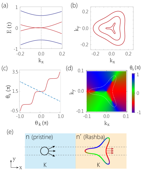
Figure 1: (Color online) (a) Band dispersion of graphene with Rashba SOC showing that the two low-energy bands (red lines) are well separated from the other bands (blue lines). (b) Constant energy contour for the low-energy bands. The TW effect is obvious. (c) Spin direction $\theta_{s}$ as a function of $\theta_{k}$ for constant energy $E_{F}=0.02\ t$. With the TW effect, the spin texture presents a terraced profile with three separated plateaus (red solid line). For comparison, we also plot the conventional spin texture of Rashba system (blue dashed line). (d) Spin direction $\theta_{s}$ in momentum space showing the plateaus in (c) persist for wide momentum range. The white dashed line is the constant energy contour for $E_{F}=0.02\ t$. (e) Schematic showing a simple way to generate current with strong spin polarization (only K valley is shown). Here, we assume $\lambda=0.2\ t$. (a) is calculated with four-band Hamiltonian $H$ (1), while (b), (c) and (d) are obtained from two-band Hamiltonian $H_{w}$ (2).

Since $H_{w}$ does not contain $\sigma_{z}$, the out-of-plane component of spin $s_{z}\propto\langle\sigma_{z}\rangle$ vanishes. Then the spin of low-energy electron lies in the plane, and its direction is given as $\theta_{s}=\arg(s_{x}+is_{y})$ with $s_{x(y)}=\langle\sigma_{x(y)}\rangle$. A straightforward calculation leads to

$$\theta_{s}=\arg(d_{x}+id_{y}),$$ (3)

with $d_{x(y)}$ the coefficients of $\sigma_{x(y)}$ in Hamiltonian (2). When Rashba SOC $\lambda$ dominates the direct hoping energy $t$, one has $H_{w}\sim k_{x}\sigma_{y}+k_{y}\sigma_{x}$ and then the spin direction of electron is normal to its $\bm{k}$ direction as $\theta_{s}=\arg(k_{y}+ik_{x})$, recovering the conventional spin texture of Rashba SOC systems Manchon et al. (2015).

III Terraced spin texture

Interestingly, when $\lambda$ is comparable with $t$ and then the TW effect becomes obvious [see Fig. 1(b)], the spin texture of system would be very different. In Fig. 1(c), we plot the spin direction of electron ($\theta_{s}$) as a function of azimuth angle of momentum $\theta_{k}$ [$\theta_{k}\equiv\arg(k_{x}+ik_{y})$] for constant energy. Compared to spin texture of conventional Rashba system [corresponding to the case of let $\gamma=0$ in Hamiltonian (2)], one observes that the TW effect brings two distinct features into the spin texture.

First, the winding number of Fermi surface (not very close to zero energy) is $2$ rather than $1$. Because when an electron moves around Fermi surface, the variation of spin direction ($\theta_{s}$) here is $4\pi$ [red solid line in Fig. 1(c)] while that in conventional Rashba system is $2\pi$ [blue dashed line in Fig. 1(c)].

Second and remarkably, the spin texture here features a terraced profile with three separated plateaus as shown in Fig. 1(c). The three plateaus locate at the three concave segments of Fermi surface, respectively [see Fig. 1(d)]. Thus, for electrons residing at the concave segments of Fermi surface, they would share similar spin direction, indicating strong spin polarization. Moreover, the plateaus and hence the strong spin polarization persist in a large momentum and energy range as shown in Fig. 1(d). This unique spin texture can not be found in other SOC materials, e.g. the surface state of topological insulator, Weyl (Dirac) semimetals and nodal line semimetal Sheng et al. (2017); Souma et al. (2011); Sheng and Nikolić (2017); Chen et al. (2017); Zhang et al. (2017). Hence, one can expect it may have distinct influence on the transport and optical properties of system Li and Carbotte (2014).

A direct application of the terraced spin texture is to generate spin-polarized current. Consider a two-dimensional junction as shown in Fig. 1(e). The left ($x<0$) region is pristine graphene and the right ($x>0$) region is the graphene with Rashba SOC. The Fermi surface of both sides of junction can be separately controlled by the bias voltage and electric potential energy. Hence, with a fine control, the transmitted electrons in $x>0$ region can be all from one concave segment of Fermi surface [see Fig. 1(e)], generating a current with strong spin polarization. Note that in above discussions, only $K$ valley is taken into account. In fact scattering process simultaneously happens at the $K^{\prime}$ valley. However, the transmitted electrons of $K^{\prime}$ valley would not reside at a concave segment of Fermi surface and hence would weaken the spin polarization of the transmitted current. Fortunately, valley filter has been experimentally realized in graphene Rycerz et al. (2007); Wu et al. (2016). Thus by applying a valley filter, one still can obtain a current with strong spin polarization.

IV Spin splitter

Next, we explore the TW effect of Rashba SOC on the transport properties of system. Consider a graphene junction as shown in Fig. 2(a), for $x<0$ ($x>d$) the pristine graphene region and for $0<x<d$ the region of graphene with Rashba SOC. To calculate the scattering, we have to resort to the four-band Hamiltonian $H$ (1), as the description of low-energy physics of pristine graphene requires a four-band model (including spin). Then, the physics of scattering can be captured by the following model

$${\cal H}(x) = H_{0}[\Theta(-x)+\Theta(x-d)]$$ (4)

$$+ (H+V_{0})[\Theta(x)-\Theta(x-d)],$$

where $H_{0}\equiv H(\lambda=0)$ is the Hamiltonian of pristine graphene, $\Theta$ the Heaviside step function and $k_{x}$ in $H_{(0)}$ is replaced by $-i\partial_{x}$, due to the absence of translation invariance along $x$-direction. Here, we also introduce the electric potential energy ($V_{0}$) in Rashba region.

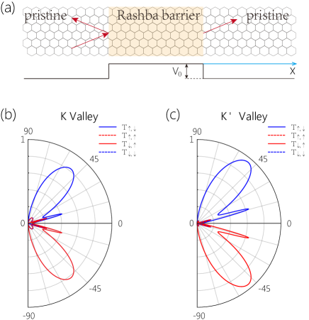
Figure 2: (Color online) (a) Schematic figure of a junction with Rashba barrier. (b)-(c) Angular plots for transmission probability $T_{s,s^{\prime}}$ as a function of incident angle $\theta_{i}$ for (b) $K$ and (c) $K^{\prime}$ valley. Here, we assume $E_{F}=0.12\ t$, $V_{0}=0.1\ t$ and $d=50\ a$.

In the scattering, the transverse momentum ($k_{y}$) and energy ($E_{F}$) are conserved while spin can be flipped when electrons pass through Rashba region. Hence, an incident electron (from $x<0$ region) with certain spin may be reflected or transmitted (into $x>d$ region) as electron with opposite spin. In addition, since the dispersion of Hamiltonian $H$ (1) contains quartic terms of $k_{x}$, there exist four possible electron states for given $k_{y}$ and $E_{F}$. Then, the typical scattering state of the junction model reads

$$\Psi(x) = \begin{cases}\psi_{s}^{+}+\sum_{s^{\prime}}r_{s^{\prime}s}\psi_{s^{\prime}}^{-},&x<0,\\ \sum_{i}c_{i}\psi_{i}^{R},&0<x<d\\ \sum_{s^{\prime}}t_{s^{\prime}s}\psi_{s^{\prime}}^{+},&x>d,\end{cases},$$ (5)

where $s(s^{\prime})=\uparrow,\downarrow$ denotes spin, $r_{ss^{\prime}}$ ($t_{ss^{\prime}}$) is the reflection (transmission) amplitude and $c_{i}$ is the scattering amplitude in Rashba region with $i=1,2,3,4$ corresponding to the four scattering states. The incident (reflected) wave function is given as $\psi_{\uparrow}^{\pm}=(\bm{0},\varphi_{\pm})^{T}e^{\pm ik_{x}^{+}x+ik_{y}y}$ for $s=\uparrow$ ($s^{\prime}=\uparrow$) and $\psi_{\downarrow}^{\pm}=(\varphi_{\pm},\bm{0})e^{\pm ik_{x}^{+}x+ik_{y}y}$ for $s=\downarrow$ ($s^{\prime}=\downarrow$). Here, $\bm{0}=(0,0)$ is a two-component vector and $\varphi_{\pm}=\frac{1}{\mathcal{N}}(\pm\sqrt{k_{x}^{+2}+k_{y}^{2}},\pm k_{x}^{+}+ik_{y})$ with $k_{x}^{+}=v_{F}^{-1}\sqrt{E-v_{F}^{2}k_{y}^{2}}$ and $\mathcal{N}$ the normalization coefficient. The corresponding scattering basis states in Rashba region and in transmitted region can be obtained by the conservation of energy and transverse momentum.

The scattering amplitudes can be solved by matching the boundary conditions at two interfaces $x=0$ and $x=d$ (see Appendix A):

$$\Psi(0^{-})=(1+{\cal U})\Psi(0^{+}), \Psi(d^{-})=(1-{\cal U})\Psi(d^{+}),$$ (6)

with

$${\cal U}=-i\frac{\sqrt{3}\lambda a}{8v_{F}}(i\tau_{y}\otimes\sigma_{0}+\tau_{x}\otimes\sigma_{z}).$$ (7)

Though analytical expressions for the scattering amplitudes are difficult to obtain, we can solve them numerically. When the scattering amplitudes are obtained, one immediately knows the reflection ($R_{s^{\prime}s}$) and transmission ($T_{s^{\prime}s}$) probability, as $R_{s^{\prime}s}=|r_{s^{\prime}s}|^{2}$ and $T_{s^{\prime}s}=|t_{s^{\prime}s}|^{2}$. Due to the presence of mirror symmetry with respect to $y$-direction (${\cal M}_{y}$), one has

$${\cal M}_{y}{\cal H}(k_{y}){\cal M}_{y}^{-1} = {\cal H}(-k_{y}),$$ (8)

with ${\cal M}_{y}=\tau_{y}\sigma_{x}$ and hence

$$T_{s,s^{\prime}}(k_{y}) = T_{-s,-s^{\prime}}(-k_{y}),$$ (9)

as ${\cal M}_{y}$ not only changes $k_{y}$ to $-k_{y}$ but also flips up (down) spin to down (up) spin. Meanwhile, there does not exist additional symmetry to guarantee $T_{s,s^{\prime}}(k_{y})=T_{s,-s^{\prime}}(k_{y})$ or $T_{s,s^{\prime}}(k_{y})=T_{-s,-s^{\prime}}(k_{y})$. Thus the transmitted current can be spin polarized as shown in Fig. 2(b). By comparison, in the previous studies of Rashba SOC without TW Bercioux and De Martino (2010), equation $T_{s,s^{\prime}}(k_{y})=T_{-s,-s^{\prime}}(k_{y})$ does have been observed due to an artificial emergent symmetry, making transmitted electrons spin degenerate, in such case, one needs to introduce additional SOC effect (e.g. intrinsic SOC) to establish spin polarization Bercioux and De Martino (2010). In contrast, we demonstrate here that when the TW effect is included only Rashba SOC is enough to achieve spin polarization, which extremely facilitates the experimental realization of spin polarization.

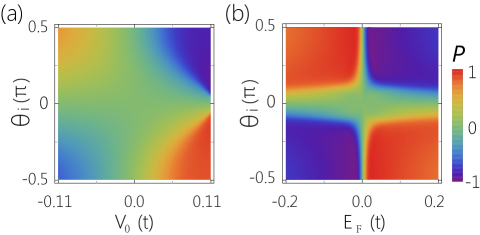
Figure 3: (Color online) Total spin polarization $P$ as a function of (a) incident angle $\theta_{i}$ and the height of potential barrier $V_{0}$, and of (b) $\theta_{i}$ and Fermi energy $E_{F}$. Here, we set $E_{F}=0.12\ t$ and $d=50\ a$ in (a), and $V_{0}=E_{F}/1.2$ and $d=50\ a$ in (b).

The above discussion of symmetry are valid for both valleys. In Fig. 2(b)-(c), we plot the transmission probabilities for both $K$ and $K^{\prime}$ valley, showing spin polarization of transmitted current can be found in both valleys. Moreover, we find that in the scattering, the spin flipping process can dominate the spin preserved process ($T_{s,-s}\gg T_{s,s}$) and is asymmetric between incident angle $\theta_{i}$ [e.g. $T_{\uparrow,\downarrow}(\theta_{i})\neq T_{\uparrow,\downarrow}(-\theta_{i})$]. Particularly, $T_{\uparrow,\downarrow}$ would peak around a certain angle $\theta_{c}^{\nu}$ [see Fig. 2(b) and 2(c)], in the mean time, $T_{\downarrow,\uparrow}$ will peak around $-\theta_{c}^{\nu}$ angle as required by the mirror symmetry [Eq. (9)]. Here $\nu=K,K^{\prime}$ denotes the valley. And, the center angles ($\theta_{c}^{\nu}$) of $T_{\uparrow,\downarrow}$ for the two valleys can be very close (see Fig. 2). Then the transmitted electron with angle around $\theta_{c}^{\nu}$ would exhibit strong spin polarization. Generally, one can introduce Bercioux and De Martino (2010)

$$P(\theta_{i}) = \sum_{\nu=K,K^{\prime}}\frac{T_{\uparrow,\downarrow}^{\nu}+T_{\uparrow,\uparrow}^{\nu}-T_{\downarrow,\downarrow}^{\nu}-T_{\downarrow,\uparrow}^{\nu}}{T_{\uparrow,\downarrow}^{\nu}+T_{\uparrow,\uparrow}^{\nu}+T_{\downarrow,\downarrow}^{\nu}+T_{\downarrow,\uparrow}^{\nu}},$$ (10)

to quantify the total spin polarization of transmitted electrons. According to the mirror symmetry ${\cal{M}}_{y}$, $P$ should be antisymmetry with respect to incident angle

$$P(\theta_{i}) = -P(-\theta_{i}).$$ (11)

Moreover, due to the emergent particle-hole symmetry in Hamiltonian $H$ (1), one also has

$$P(\theta_{i},E_{F}+V_{0}) = P(-\theta_{i},-E_{F}-V_{0}).$$ (12)

In Fig. 3, we present the evolution of $P$ varying with potential energy and Fermi energy, which shows the spin polarization of transmitted current is strong and features aforementioned symmetries. Remarkably, nearly perfect spin polarization (e.g. $|P|>0.9$) can happen in a wide $E_{F}$ and $V_{0}$ energy scale.

Due to the antisymmetry of $P$ [Eq. (11)], a usual two terminals device is not valid to probe to the polarization effect as an average over incident angle $\theta_{i}$ is involved. Alternatively, one can use a ${\rm Y}$-type structure (see Fig. 4) for splitting transmitted current. In the ${\rm Y}$-type junction, the currents moving through drain A and B can present strong and opposite spin polarization as guaranteed by Eq. (11), making the realization of spin splitter. Also, by changing the sign of $E_{F}$ and $V_{0}$ simultaneously, one can switch the sign of $P$ [Eq. (12)] and hence switch the spin polarization of current in drain A and B (see Fig. 4). In addition, with more delicate setups, e.g. by applying collimators similar to those in electron optics, one could control the incident angle. Then by tuning electrical potential energy or Fermi energy, a nearly perfect spin polarization current could be observed.

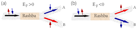
Figure 4: (Color online) Schematic figure showing the Y-type structure for achieving spin splitter. (a) For electron doping ($E_{F}>0$ and $V_{0}=E_{F}/1.2$), the down-spin (up-spin) of the current passing through drain A (B) can dominate up-spin (down-spin). (b) For hole doping ($E_{F}<0$ and $V_{0}=E_{F}/1.2$), the spin polarization of transmitted current is switched.

V Conclusion

In conclusion, we have predicted two intriguing features induced by the TW effect in Rashba SOC. The terraced spin texture at Fermi surface predicted here is unique and can not be found in other SOC materials. Particularly, the spin texture here is related to real spin. Thus, it may be detected by the spin- and angle-resolved photoemission (spinARPES). In addition, the terraced spin texture can be used to generate current with strong spin polarization. We also study the scattering of system with a Rashba barrier and observe strong spin polarization in the transmitted current. The spin polarization is solely induced by Rashba SOC and can be controlled by electric method (tuning $V_{0}$ and $E_{F}$). And, with a Y-structure junction (see Fig. 4), one can establish a spin splitter. Our work indicates that the warping effect of Fermi surface, together with SOC, can give rise to many interesting phenomena which may be helpful to the spintronics.

Appendix A Boundary Condition

Due to the presence of $\lambda k_{x(y)}$ in Hamiltonian $H$ (1), the boundary conditions for the graphene junction with Rashba barrier generally can not be expressed as the continuum of wavefunction at interfaces $x=0$ and $x=d$. Here, we establish the boundary conditions of the junction model (4) in detail.

The junction model (4) in main text with basis $(|A\downarrow\rangle,|B\downarrow\rangle,|A\uparrow\rangle,|B\uparrow\rangle)^{T}$ can be written as

$${\cal H}(x) = \left(\begin{array}[]{cccc}0&v_{F}k_{-}&0&h_{0}\\ v_{F}k_{+}&0&h_{1}&0\\ 0&h_{1}^{*}&0&v_{F}k_{-}\\ h_{0}^{*}&0&v_{F}k_{+}&0\end{array}\right),$$ (17)

where $k_{\pm}=k_{x}\pm ik_{y}$, $\lambda(x)=\lambda\Theta(x)$ and

$$h_{0} = 3i\lambda\left(x\right),$$ (18)

$$h_{1} = -i\frac{\sqrt{3}}{2}a\lambda\left(x\right)k_{-}.$$ (19)

The eigenfunction of system is ${\cal H}(x)\Psi\left(x\right)=E\Psi\left(x\right)$ with $E$ the eigenvalue and $\Psi\left(x\right)=\left(\psi_{1},\ \psi_{2},\ \psi_{3},\ \psi_{4}\ \right)^{T}$ the eigenfunction. Because the eigenfunction $\Psi\left(x\right)$ and eigenvalue $E$ are finite, one has

$$\int_{0^{-}}^{0^{+}}{\cal H}(x)\Psi(x)dx = \int_{0^{-}}^{0^{+}}E\Psi(x)dx=0,$$ (20)

$$\int_{d+0^{-}}^{d+0^{+}}{\cal H}(x)\Psi(x)dx = \int_{d+0^{-}}^{d+0^{+}}E\Psi(x)dx=0.$$ (21)

The boundary conditions can be established from above equations. A straightforward calculation gives that $\psi_{2(3)}(x)$ is continuum at interfaces ($x=0$ and $x=d$) while

$$\psi_{1}(0^{+})-\psi_{1}(0^{-}) = i\xi\psi_{3}(0),$$ (22)

$$\psi_{4}(0^{+})-\psi_{4}(0^{-}) = -i\xi\psi_{2}(0),$$ (23)

$$\psi_{1}(d+0^{+})-\psi_{1}(d+0^{-}) = -i\xi\psi_{3}(d),$$ (24)

$$\psi_{4}(d+0^{+})-\psi_{4}(d+0^{-}) = i\xi\psi_{2}(d),$$ (25)

with $\xi=\frac{\sqrt{3}\lambda a}{4v_{F}}$. The above equations are the boundary conditions of system and the compact forms have been given in Eq (6) of main text. One can check that with such boundary conditions, current conservation is satisfied.

References

- Chiu et al. (2016) C.-K. Chiu, J. C. Y. Teo, A. P. Schnyder, and S. Ryu, Rev. Mod. Phys. 88, 035005 (2016).
- Wolf et al. (2001) S. Wolf, D. Awschalom, R. Buhrman, J. Daughton, S. Von Molnar, M. Roukes, A. Y. Chtchelkanova, and D. Treger, Science 294, 1488 (2001).
- Žutić et al. (2004) I. Žutić, J. Fabian, and S. D. Sarma, Rev. Mod. Phys. 76, 323 (2004).
- Pulizzi (2012) F. Pulizzi, Nat. Mater. 11, 367 (2012).
- Dyrdał et al. (2009) A. Dyrdał, V. Dugaev, and J. Barnaś, Phys. Rev. B 80, 155444 (2009).
- Jungwirth et al. (2016) T. Jungwirth, X. Marti, P. Wadley, J. Wunderlich, et al., Nat Nanotechnol. 11, 231 (2016).
- Eichler et al. (2017) C. Eichler, A. Sigillito, S. Lyon, and J. Petta, Phys. Rev. Lett. 118, 037701 (2017).
- Yazyev and Katsnelson (2008) O. V. Yazyev and M. Katsnelson, Phys. Rev. Lett. 100, 047209 (2008).
- Wang et al. (2005) J. Wang, H. Meng, and J.-P. Wang, J. Appl. Polym. Sci. 97, 10D509 (2005).
- Pientka et al. (2017) F. Pientka, J. Waissman, P. Kim, and B. I. Halperin, Phys. Rev. Lett. 119, 027601 (2017).
- Liu et al. (2016) D.-P. Liu, Z.-M. Yu, and Y.-L. Liu, Phys. Rev. B 94, 155112 (2016).
- Engels et al. (1997) G. Engels, J. Lange, T. Schäpers, and H. Lüth, Phys. Rev. B 55, R1958 (1997).
- Ohe et al. (2005) J.-i. Ohe, M. Yamamoto, T. Ohtsuki, and J. Nitta, Phys. Rev. B 72, 041308 (2005).
- Yamamoto et al. (2005) M. Yamamoto, T. Ohtsuki, and B. Kramer, Phys. Rev. B 72, 115321 (2005).
- Zhao et al. (2016) J. Zhao, H. Liu, Z. Yu, R. Quhe, S. Zhou, Y. Wang, C. C. Liu, H. Zhong, N. Han, J. Lu, Y. Yao, and K. Wu, Prog. Mater. Sci. 83, 24 (2016).
- Kormányos et al. (2013) A. Kormányos, V. Zólyomi, N. D. Drummond, P. Rakyta, G. Burkard, and V. I. Fal’ko, Phys. Rev. B 88, 045416 (2013).
- Rakyta et al. (2010) P. Rakyta, A. Kormanyos, and J. Cserti, Phys. Rev. B 82, 113405 (2010).
- Yu et al. (2015) Z. Yu, H. Pan, and Y. Yao, Phys. Rev. B 92, 155419 (2015).
- Fu (2009) L. Fu, Phys. Rev. Lett. 103, 266801 (2009).
- Yu et al. (2017) Z.-M. Yu, D.-S. Ma, H. Pan, and Y. Yao, Phys. Rev. B 96, 125152 (2017).
- Yokoyama (2013) T. Yokoyama, Phys. Rev. B 87, 241409 (2013).
- Tsai et al. (2013) W.-F. Tsai, C.-Y. Huang, T.-R. Chang, H. Lin, H.-T. Jeng, and A. Bansil, Nat. Commun. 4, 1500 (2013).
- Beenakker (2008) C. Beenakker, Rev. Mod. Phys. 80, 1337 (2008).
- Tombros et al. (2012) N. Tombros, C. Jozsa, M. Popinciuc, H. T. Jonkman, and B. J. van Wees, Phys. Rev. B 85, 085406 (2012).
- Grujić et al. (2014) M. M. Grujić, M. Ž. Tadić, and F. M. Peeters, Phys. Rev. Lett. 113, 046601 (2014).
- Habe and Koshino (2015) T. Habe and M. Koshino, Phys. Rev. B 91, 201407 (2015).
- Xiao et al. (2007) D. Xiao, W. Yao, and Q. Niu, Phys. Rev. Lett. 99, 236809 (2007).
- Marchenko et al. (2012) D. Marchenko, A. Varykhalov, M. Scholz, G. Bihlmayer, E. Rashba, A. Rybkin, A. Shikin, and O. Rader, Nat. Commun. 3, 1232 (2012).
- Ishizaka et al. (2011) K. Ishizaka, M. Bahramy, H. Murakawa, M. Sakano, T. Shimojima, T. Sonobe, K. Koizumi, S. Shin, H. Miyahara, A. Kimura, et al., Nat. Mater. 10, 521 (2011).
- Eremeev et al. (2012) S. V. Eremeev, I. A. Nechaev, Y. M. Koroteev, P. M. Echenique, and E. V. Chulkov, Phys. Rev. Lett. 108, 246802 (2012).
- Varykhalov et al. (2012) A. Varykhalov, D. Marchenko, M. Scholz, E. Rienks, T. Kim, G. Bihlmayer, J. Sánchez-Barriga, and O. Rader, Phy. Rev. Lett. 108, 066804 (2012).
- Di Sante et al. (2013) D. Di Sante, P. Barone, R. Bertacco, and S. Picozzi, Adv. Mater. 25, 509 (2013).
- Liebmann et al. (2016) M. Liebmann, C. Rinaldi, D. Di Sante, J. Kellner, C. Pauly, R. N. Wang, J. E. Boschker, A. Giussani, S. Bertoli, M. Cantoni, et al., Adv. Mater. 28, 560 (2016).
- Matetskiy et al. (2015) A. Matetskiy, S. Ichinokura, L. Bondarenko, A. Tupchaya, D. Gruznev, A. Zotov, A. Saranin, R. Hobara, A. Takayama, and S. Hasegawa, Phys. Rev. Lett. 115, 147003 (2015).
- Volobuev et al. (2017) V. V. Volobuev, P. S. Mandal, M. Galicka, O. Caha, J. Sánchez-Barriga, D. Di Sante, A. Varykhalov, A. Khiar, S. Picozzi, G. Bauer, et al., Adv. Mater. 29, 1604185 (2017).
- Niesner et al. (2016) D. Niesner, M. Wilhelm, I. Levchuk, A. Osvet, S. Shrestha, M. Batentschuk, C. Brabec, and T. Fauster, Phys. Rev. Lett. 117, 126401 (2016).
- Kane and Mele (2005) C. L. Kane and E. J. Mele, Phys. Rev. Lett. 95, 226801 (2005).
- Bercioux and De Martino (2010) D. Bercioux and A. De Martino, Phys. Rev. B 81, 165410 (2010).
- Manchon et al. (2015) A. Manchon, H. C. Koo, J. Nitta, S. M. Frolov, and R. A. Duine, Nat Mater 14, 871 (2015).
- Sheng et al. (2017) X.-L. Sheng, Z.-M. Yu, R. Yu, H. Weng, and S. A. Yang, Jour. Phys. Chem. Lett. 8, 3506 (2017).
- Souma et al. (2011) S. Souma, K. Kosaka, T. Sato, M. Komatsu, A. Takayama, T. Takahashi, M. Kriener, K. Segawa, and Y. Ando, Phys. Rev. Lett. 106, 216803 (2011).
- Sheng and Nikolić (2017) X.-L. Sheng and B. K. Nikolić, Phys. Rev. B 95, 201402 (2017).
- Chen et al. (2017) C. Chen, S.-S. Wang, L. Liu, Z.-M. Yu, X.-L. Sheng, Z. Chen, and S. A. Yang, Phys. Rev. Mat. 1, 044201 (2017).
- Zhang et al. (2017) X. Zhang, L. Jin, X. Dai, and G. Liu, J. Phys. Chem. Lett. 8, 4814 (2017).
- Li and Carbotte (2014) Z. Li and J. P. Carbotte, Phys. Rev. B 89, 165420 (2014).
- Rycerz et al. (2007) A. Rycerz, J. Tworzydlo, and C. Beenakker, Nat. Phys. 3, 172 (2007).
- Wu et al. (2016) Q.-P. Wu, Z.-F. Liu, A.-X. Chen, X.-B. Xiao, and Z.-M. Liu, Sci. Rep. 6, 21590 (2016).