Higher-Order Program Verification
via HFL Model Checking

Abstract

There are two kinds of higher-order extensions of model checking: HORS model checking and HFL model checking. Whilst the former has been applied to automated verification of higher-order functional programs, applications of the latter have not been well studied. In the present paper, we show that various verification problems for functional programs, including may/must-reachability, trace properties, and linear-time temporal properties (and their negations), can be naturally reduced to (extended) HFL model checking. The reductions yield a sound and complete logical characterization of those program properties. Compared with the previous approaches based on HORS model checking, our approach provides a more uniform, streamlined method for higher-order program verification.

1 Introduction

There are two kinds of higher-order extensions of model checking in the literature: HORS model checking [18, 34] and HFL model checking [46]. The former is concerned about whether the tree generated by a given higher-order tree grammar called a higher-order recursion scheme (HORS) satisfies the property expressed by a given modal $\mu$-calculus formula (or a tree automaton), and the latter is concerned about whether a given finite state system satisfies the property expressed by a given formula of higher-order modal fixpoint logic (HFL), a higher-order extension of the modal $\mu$-calculus. Whilst HORS model checking has been applied to automated verification of higher-order functional programs [19, 20, 25, 35, 45, 28, 47], there have been few studies on applications of HFL model checking to program/system verification. Despite that HFL has been introduced more than 10 years ago, we are only aware of applications to assume-guarantee reasoning [46] and process equivalence checking [30].

In the present paper, we show that various verification problems for higher-order functional programs can actually be reduced to (extended) HFL model checking in a rather natural manner. We briefly explain the idea of our reduction below. We translate a program to an HFL formula that says “the program has a valid behavior” (where the validity of a behavior depends on each verification problem). Thus, a program is actually mapped to a property, and a program property is mapped to a system to be verified; this has been partially inspired by the recent work of Kobayashi et al. [21], where HORS model checking problems have been translated to HFL model checking problems by switching the roles of models and properties.

For example, consider a simple program fragment $\mathtt{read}(x);\mathtt{close}(x)$ that reads and then closes a file (pointer) $x$. The transition system in Figure 1 shows a valid access protocol to read-only files. Then, the property that a read operation is allowed in the current state can be expressed by a formula of the form $\langle{\mathtt{read}}\rangle\varphi$, which says that the current state has a $\mathtt{read}$-transition, after which $\varphi$ is satisfied. Thus, the program $\mathtt{read}(x);\mathtt{close}(x)$ being valid is expressed as $\langle{\mathtt{read}}\rangle\langle{\mathtt{close}}\rangle\mathbf{true}$, which is indeed satisfied by the initial state $q_{0}$ of the transition system in Figure 1. Here, we have just replaced the operations $\mathtt{read}$ and $\mathtt{close}$ of the program with the corresponding modal operators $\langle{\mathtt{read}}\rangle$ and $\langle{\mathtt{close}}\rangle$. We can also naturally deal with branches and recursions. For example, consider the program $\mathtt{close}(x)\Box(\mathtt{read}(x);\mathtt{close}(x))$, where $e_{1}\Box e_{2}$ represents a non-deterministic choice between $e_{1}$ and $e_{2}$. Then the property that the program always accesses $x$ in a valid manner can be expressed by $(\langle{\mathtt{close}}\rangle\mathbf{true})\land(\langle{\mathtt{read}}\rangle\langle{\mathtt{close}}\rangle\mathbf{true})$. Note that we have just replaced the non-deterministic branch with the logical conjunction, as we wish here to require that the program’s behavior is valid in both branches. We can also deal with conditional branches if HFL is extended with predicates; $\mathbf{if}\ b\ \mathbf{then}\ \mathtt{close}(x)\ \mathbf{else}\ {(\mathtt{read}(x);\mathtt{close}(x))}$ can be translated to $(b\Rightarrow\langle{\mathtt{close}}\rangle\mathbf{true})\land(\neg b\Rightarrow\langle{\mathtt{read}}\rangle\langle{\mathtt{close}}\rangle\mathbf{true})$. Let us also consider the recursive function $f$ defined by:

$${f\,x}={\mathtt{close}(x)\Box(\mathtt{read}(x);\mathtt{read}(x);fx)},$$

Then, the program $f\,x$ being valid can be represented by using a (greatest) fixpoint formula:

$$\nu F.(\langle{\mathtt{close}}\rangle\mathbf{true})\land(\langle{\mathtt{read}}\rangle\langle{\mathtt{read}}\rangle F).$$

If the state $q_{0}$ satisfies this formula (which is indeed the case), then we know that all the file accesses made by $f\,x$ are valid. So far, we have used only the modal $\mu$-calculus formulas. If we wish to express the validity of higher-order programs, we need HFL formulas; such examples are given later.

Figure 1: File access protocol

We generalize the above idea and formalize reductions from various classes of verification problems for simply-typed higher-order functional programs with recursion, integers and non-determinism – including verification of may/must-reachability, trace properties, and linear-time temporal properties (and their negations) – to (extended) HFL model checking where HFL is extended with integer predicates, and prove soundness and completeness of the reductions. Extended HFL model checking problems obtained by the reductions are (necessarily) undecidable in general, but for finite-data programs (i.e., programs that consist of only functions and data from finite data domains such as Booleans), the reductions yield pure HFL model checking problems, which are decidable [46].

Our reductions provide sound and complete logical characterizations of a wide range of program properties mentioned above. Nice properties of the logical characterizations include: (i) (like verification conditions for Hoare triples,) once the logical characterization is obtained as an HFL formula, purely logical reasoning can be used to prove or disprove it (without further referring to the program semantics); for that purpose, one may use theorem provers with various degrees of automation, ranging from interactive ones like Coq, semi-automated ones requiring some annotations, to fully automated ones (though the latter two are yet to be implemented), (ii) (unlike the standard verification condition generation for Hoare triples using invariant annotations) the logical characterization can automatically be computed, without any annotations, (iii) standard logical reasoning can be applied based on the semantics of formulas; for example, co-induction and induction can be used for proving $\nu$- and $\mu$-formulas respectively, and (iv) thanks to the completeness, the set of program properties characterizable by HFL formula is closed under negations; for example, from a formula characterizing may-reachability, one can obtain a formula characterizing non-reachability by just taking the De Morgan dual.

Compared with previous approaches based on HORS model checking [20, 25, 35, 41, 28], our approach based on (extended) HFL model checking provides more uniform, streamlined methods for higher-order program verification. HORS model checking provides sound and complete verification methods for finite-data programs [19, 20], but for infinite-data programs, other techniques such as predicate abstraction [25] and program transformation [29, 33] had to be combined to obtain sound (but incomplete) reductions to HORS model checking. Furthermore, the techniques were different for each of program properties, such as reachability [25], termination [29], non-termination [28], fair termination [33], and fair non-termination [47]. In contrast, our reductions are sound and complete even for infinite-data programs. Although the obtained HFL model checking problems are undecidable in general, the reductions allow us to treat various program properties uniformly; all the verifications are boiled down to the issue of how to prove $\mu$- and $\nu$-formulas (and as remarked above, we can use induction and co-induction to deal with them). Technically, our reduction to HFL model checking may actually be considered an extension of HORS model checking in the following sense. HORS model checking algorithms [34, 23] usually consist of two phases, one for computing a kind of higher-order “procedure summaries” in the form of variable profiles [34] or intersection types [23], and the other for nested least/greatest fixpoint computations. Our reduction from program verification to extended HFL model checking (the reduction given in Section 7, in particular) can be regarded as an extension of the first phase to deal with infinite data domains, where the problem for the second phase is expressed in the form of extended HFL model checking: see Appendix 0.H for more details.

The rest of this paper is structured as follows. Section 2 introduces HFL extended with integer predicates and defines the HFL model checking problem. Section 3 informally demonstrates some examples of reductions from program verification problems to HFL model checking. Section 4 introduces a functional language used to formally discuss the reductions in later sections. Sections 5, 6, and 7 consider may/must-reachability, trace properties, and temporal properties respectively, and present (sound and complete) reductions from verification of those properties to HFL model checking. Section 8 discusses related work, and Section 9 concludes the paper. Proofs are found in Appendices.

2 (Extended) HFL

In this section, we introduce an extension of higher-order modal fixpoint logic (HFL) [46] with integer predicates (which we call HFL_Z; we often drop the subscript and just write HFL, as in Section 1), and define the HFL_Z model checking problem. The set of integers can actually be replaced by another infinite set $X$ of data (like the set of natural numbers or the set of finite trees) to yield HFL_X.

2.1 Syntax

For a map $f$, we write $\mathit{dom}(f)$ and $\mathit{codom}(f)$ for the domain and codomain of $f$ respectively. We write $\mathbf{Z}$ for the set of integers, ranged over by the meta-variable $n$ below. We assume a set $\mathbf{Pred}$ of primitive predicates on integers, ranged over by $p$. We write $\mathtt{arity}(p)$ for the arity of $p$. We assume that $\mathbf{Pred}$ contains standard integer predicates such as $=$ and $<$, and also assume that, for each predicate $p\in\mathbf{Pred}$, there also exists a predicate $\neg p\in\mathbf{Pred}$ such that, for any integers $n_{1},\ldots,n_{k}$, $p(n_{1},\ldots,n_{k})$ holds if and only if $\neg p(n_{1},\ldots,n_{k})$ does not hold; thus, $\neg p(n_{1},\ldots,n_{k})$ should be parsed as $(\neg p)(n_{1},\ldots,n_{k})$, but can semantically be interpreted as $\neg(p(n_{1},\ldots,n_{k}))$.

The syntax of HFL_Z formulas is given by:

$$\begin{array}[]{l}\varphi\mbox{ (formulas) }::=n\mid\varphi_{1}\mathbin{\mathtt{op}}\varphi_{2}\mid\mathbf{true}\mid\mathbf{false}\mid p(\varphi_{1},\ldots,\varphi_{k})\mid\varphi_{1}\vee\varphi_{2}\mid\varphi_{1}\wedge\varphi_{2}\\ \qquad\qquad\qquad\mid X\mid\langle{a}\rangle\varphi\mid[a]\varphi\mid\mu X^{\tau}.\varphi\mid\nu X^{\tau}.\varphi\mid\lambda X\mathbin{:}{\sigma}.\varphi\mid\varphi_{1}\;\varphi_{2}\\ \tau\mbox{ (types) }::=\bullet\mid\sigma\to\tau\qquad\sigma\mbox{ (extended types) }::=\tau\mid\mathtt{int}\end{array}$$

Here, $\mathbin{\mathtt{op}}$ ranges over a set of binary operations on integers, such as $+$, and $X$ ranges over a denumerable set of variables. We have extended the original HFL [46] with integer expressions ($n$ and $\varphi_{1}\mathbin{\mathtt{op}}\varphi_{2}$), and atomic formulas $p(\varphi_{1},\ldots,\varphi_{k})$ on integers (here, the arguments of integer operations or predicates will be restricted to integer expressions by the type system introduced below). Following [21], we have omitted negations, as any formula can be transformed to an equivalent negation-free formula [32].

We explain the meaning of each formula informally; the formal semantics is given in Section 2.2. Like modal $\mu$-calculus [27, 11], each formula expresses a property of a labeled transition system. The first line of the syntax of formulas consists of the standard constructs of predicate logics. On the second line, as in the standard modal $\mu$-calculus, $\langle{a}\rangle\varphi$ means that there exists an $a$-labeled transition to a state that satisfies $\varphi$. The formula $[a]\varphi$ means that after any $a$-labeled transition, $\varphi$ is satisfied. The formulas $\mu X^{\tau}.\varphi$ and $\nu X^{\tau}.\varphi$ represent the least and greatest fixpoints respectively (the least and greatest $X$ that $X=\varphi$) respectively; unlike the modal $\mu$-calculus, $X$ may range over not only propositional variables but also higher-order predicate variables (of type $\tau$). The $\lambda$-abstractions $\lambda X\mathbin{:}{\sigma}.\varphi$ and applications $\varphi_{1}\;\varphi_{2}$ are used to manipulate higher-order predicates. We often omit type annotations in $\mu X^{\tau}.\varphi$, $\nu X^{\tau}.\varphi$ and $\lambda X\mathbin{:}{\sigma}.\varphi$, and just write $\mu X.\varphi$, $\nu X.\varphi$ and $\lambda X.\varphi$.

Example 1

Consider $\varphi_{\mathtt{ab}}\,\varphi$ where $\varphi_{\mathtt{ab}}=\mu X^{\bullet\to\bullet}.\lambda Y\mathbin{:}\bullet.Y\lor\langle{\mathtt{a}}\rangle(X(\langle{\mathtt{b}}\rangle Y))$. We can expand the formula as follows:

$$\begin{array}[]{l}\varphi_{\mathtt{ab}}\,\varphi=(\lambda Y.\bullet.Y\lor\langle{\mathtt{a}}\rangle(\varphi_{\mathtt{ab}}(\langle{\mathtt{b}}\rangle Y)))\varphi=\varphi\lor\langle{\mathtt{a}}\rangle(\varphi_{\mathtt{ab}}(\langle{\mathtt{b}}\rangle\varphi))\\ \qquad=\varphi\lor\langle{\mathtt{a}}\rangle(\langle{\mathtt{b}}\rangle\varphi\lor\langle{\mathtt{a}}\rangle(\varphi_{\mathtt{ab}}(\langle{\mathtt{b}}\rangle\langle{\mathtt{b}}\rangle\varphi)))=\cdots,\end{array}$$

and obtain $\varphi\lor(\langle{\mathtt{a}}\rangle\langle{\mathtt{b}}\rangle\varphi)\lor(\langle{\mathtt{a}}\rangle\langle{\mathtt{a}}\rangle\langle{\mathtt{b}}\rangle\langle{\mathtt{b}}\rangle\varphi)\lor\cdots$. Thus, the formula means that there is a transition sequence of the form $\mathtt{a}^{n}\mathtt{b}^{n}$ for some $n\geq 0$ that leads to a state satisfying $\varphi$.

Following [21], we exclude out unmeaningful formulas such as $(\langle{a}\rangle\mathbf{true})+1$ by using a simple type system. The types $\bullet$, $\mathtt{int}$, and $\sigma\to\tau$ describe propositions, integers, and (monotonic) functions from $\sigma$ to $\tau$, respectively. Note that the integer type $\mathtt{int}$ may occur only in an argument position; this restriction is required to ensure that least and greatest fixpoints are well-defined. The typing rules for formulas are given in Figure 2. In the figure, $\Delta$ denotes a type environment, which is a finite map from variables to (extended) types. Below we consider only well-typed formulas, i.e., formulas $\varphi$ such that $\Delta\vdash_{\mathtt{H}}\varphi:\tau$ for some $\Delta$ and $\tau$.

$\displaystyle\frac{\begin{array}[]{@{}c@{}}\end{array}}{\begin{array}[]{@{}c@{}}\Delta\vdash_{\mathtt{H}}n:\mathtt{int}\end{array}}$ (HT-Int)

$\displaystyle\frac{\begin{array}[]{@{}c@{}}\Delta\vdash_{\mathtt{H}}\varphi_{i}:\mathtt{int}\mbox{ for each $i\in\{1,2\}$}\end{array}}{\begin{array}[]{@{}c@{}}\Delta\vdash_{\mathtt{H}}\varphi_{1}\mathbin{\mathtt{op}}\varphi_{2}:\mathtt{int}\end{array}}$ (HT-Op)

$\displaystyle\frac{\begin{array}[]{@{}c@{}}\end{array}}{\begin{array}[]{@{}c@{}}\Delta\vdash_{\mathtt{H}}\mathbf{true}:\bullet\end{array}}$ (HT-True)

$\displaystyle\frac{\begin{array}[]{@{}c@{}}\end{array}}{\begin{array}[]{@{}c@{}}\Delta\vdash_{\mathtt{H}}\mathbf{false}:\bullet\end{array}}$ (HT-False)

$\displaystyle\frac{\begin{array}[]{@{}c@{}}\mathtt{arity}(p)=k\\ \Delta\vdash_{\mathtt{H}}\varphi_{i}:\mathtt{int}\mbox{ for each $i\in\{1,\ldots,k\}$}\end{array}}{\begin{array}[]{@{}c@{}}\Delta\vdash_{\mathtt{H}}p(\varphi_{1},\ldots,\varphi_{k}):\bullet\end{array}}$ (HT-Pred)

$\displaystyle\frac{\begin{array}[]{@{}c@{}}\end{array}}{\begin{array}[]{@{}c@{}}\Delta,X\mathbin{:}\sigma\vdash_{\mathtt{H}}X:\sigma\end{array}}$ (HT-Var)

$\displaystyle\frac{\begin{array}[]{@{}c@{}}\Delta\vdash_{\mathtt{H}}\varphi_{i}:\bullet\mbox{ for each $i\in\{1,2\}$}\end{array}}{\begin{array}[]{@{}c@{}}\Delta\vdash_{\mathtt{H}}\varphi_{1}\vee\varphi_{2}:\bullet\end{array}}$ (HT-Or)

$\displaystyle\frac{\begin{array}[]{@{}c@{}}\Delta\vdash_{\mathtt{H}}\varphi_{i}:\bullet\mbox{ for each $i\in\{1,2\}$}\end{array}}{\begin{array}[]{@{}c@{}}\Delta\vdash_{\mathtt{H}}\varphi_{1}\wedge\varphi_{2}:\bullet\end{array}}$ (HT-And)

$\displaystyle\frac{\begin{array}[]{@{}c@{}}\Delta\vdash_{\mathtt{H}}\varphi:\bullet\end{array}}{\begin{array}[]{@{}c@{}}\Delta\vdash_{\mathtt{H}}\langle{a}\rangle\varphi:\bullet\end{array}}$ (HT-Some)

$\displaystyle\frac{\begin{array}[]{@{}c@{}}\Delta\vdash_{\mathtt{H}}\varphi:\bullet\end{array}}{\begin{array}[]{@{}c@{}}\Delta\vdash_{\mathtt{H}}[a]\varphi:\bullet\end{array}}$ (HT-All)

$\displaystyle\frac{\begin{array}[]{@{}c@{}}\Delta,X:\tau\vdash_{\mathtt{H}}\varphi:\tau\end{array}}{\begin{array}[]{@{}c@{}}\Delta\vdash_{\mathtt{H}}\mu X^{\tau}.\ \varphi:\tau\end{array}}$ (HT-Mu)

$\displaystyle\frac{\begin{array}[]{@{}c@{}}\Delta,X:\tau\vdash_{\mathtt{H}}\varphi:\tau\end{array}}{\begin{array}[]{@{}c@{}}\Delta\vdash_{\mathtt{H}}\nu X^{\tau}.\ \varphi:\tau\end{array}}$ (HT-Nu)

$\displaystyle\frac{\begin{array}[]{@{}c@{}}\Delta,X:\sigma\vdash_{\mathtt{H}}\varphi:\tau\end{array}}{\begin{array}[]{@{}c@{}}\Delta\vdash_{\mathtt{H}}\lambda X\mathbin{:}{\sigma}.\ \varphi:\sigma\to\tau\end{array}}$ (HT-Abs)

$\displaystyle\frac{\begin{array}[]{@{}c@{}}\Delta\vdash_{\mathtt{H}}\varphi_{1}:\sigma\to\tau\quad\Delta\vdash_{\mathtt{H}}\varphi_{2}:\sigma\end{array}}{\begin{array}[]{@{}c@{}}\Delta\vdash_{\mathtt{H}}\varphi_{1}\ \varphi_{2}:\tau\end{array}}$ (HT-App)

Figure 2: Typing Rules for HFL_Z Formulas

2.2 Semantics and HFL_Z Model Checking

We now define the formal semantics of HFL_Z formulas. A labeled transition system (LTS) is a quadruple $\mathtt{L}=(U{},A{},\mathbin{\mathbin{\longrightarrow}},\mathtt{s}_{\mathtt{init}})$, where $U{}$ is a finite set of states, $A{}$ is a finite set of actions, $\mathbin{\mathbin{\longrightarrow}}\subseteq U{}\times A{}\times U$ is a labeled transition relation, and $\mathtt{s}_{\mathtt{init}}\in U$ is the initial state. We write $\mathtt{s}_{1}\stackrel{{\scriptstyle a}}{{\mathbin{\longrightarrow}}}\mathtt{s}_{2}$ when $(\mathtt{s}_{1},a,\mathtt{s}_{2})\in\mathbin{\longrightarrow}$.

For an LTS $\mathtt{L}=(U{},A{},\mathbin{\mathbin{\longrightarrow}},\mathtt{s}_{\mathtt{init}})$ and an extended type $\sigma$, we define the partially ordered set $(\mathcal{D}_{\mathtt{L},\sigma},\sqsubseteq_{\mathtt{L},\sigma})$ inductively by:

$$\begin{array}[]{l}\mathcal{D}_{\mathtt{L},\bullet}={2^{U}}\qquad\sqsubseteq_{\mathtt{L},\bullet}=\subseteq\qquad\mathcal{D}_{\mathtt{L},\mathtt{int}}=\mathbf{Z}\qquad\sqsubseteq_{\mathtt{L},\mathtt{int}}=\{(n,n)\mid n\in\mathbf{Z}\}\\ \mathcal{D}_{\mathtt{L},\sigma\to\tau}=\{f\in\mathcal{D}_{\mathtt{L},\sigma}\to\mathcal{D}_{\mathtt{L},\tau}\mid\forall x,y.(x\sqsubseteq_{\mathtt{L},\sigma}y\Rightarrow f\,x\sqsubseteq_{\mathtt{L},\tau}f\,y)\}\\ \sqsubseteq_{\mathtt{L},\sigma\to\tau}=\{(f,g)\mid\forall x\in\mathcal{D}_{\mathtt{L},\sigma}.f(x)\sqsubseteq_{\mathtt{L},\tau}g(x)\}\end{array}$$

Note that $(\mathcal{D}_{\mathtt{L},\tau},\sqsubseteq_{\mathtt{L},\tau})$ forms a complete lattice (but $(\mathcal{D}_{\mathtt{L},\mathtt{int}},\sqsubseteq_{\mathtt{L},\mathtt{int}})$ does not). We write $\bot_{\mathtt{L},\tau}$ and $\top_{\mathtt{L},\tau}$ for the least and greatest elements of $\mathcal{D}_{\mathtt{L},\tau}$ (which are $\lambda\widetilde{x}.\emptyset$ and $\lambda\widetilde{x}.U$) respectively. We sometimes omit the subscript $\mathtt{L}$ below. Let $\llbracket\Delta\rrbracket_{\mathtt{L}}$ be the set of functions (called valuations) that maps $X$ to an element of $\mathcal{D}_{\mathtt{L},\sigma}$ for each $X\mathbin{:}\sigma\in\Delta$. For an HFL formula $\varphi$ such that $\Delta\vdash_{\mathtt{H}}\varphi:\sigma$, we define $\llbracket\Delta\vdash_{\mathtt{H}}\varphi:\sigma\rrbracket_{\mathtt{L}}$ as a map from $\llbracket\Delta\rrbracket_{\mathtt{L}}$ to $\mathcal{D}_{\sigma}$, by induction on the derivation of $\Delta\vdash_{\mathtt{H}}\varphi:\sigma$, as follows.

$$\llbracket\Delta\vdash_{\mathtt{H}}n:\mathtt{int}\rrbracket_{\mathtt{L}}(\rho)=n\qquad\llbracket\Delta\vdash_{\mathtt{H}}\mathbf{true}:\bullet\rrbracket_{\mathtt{L}}(\rho)=U\qquad\llbracket\Delta\vdash_{\mathtt{H}}\mathbf{false}:\bullet\rrbracket_{\mathtt{L}}(\rho)=\emptyset$$

$$\llbracket\Delta\vdash_{\mathtt{H}}\varphi_{1}\mathbin{\mathtt{op}}\varphi_{2}:\mathtt{int}\rrbracket_{\mathtt{L}}(\rho)=(\llbracket\Delta\vdash_{\mathtt{H}}\varphi_{1}:\mathtt{int}\rrbracket_{\mathtt{L}}(\rho))\llbracket\mathbin{\mathtt{op}}\rrbracket(\llbracket\Delta\vdash_{\mathtt{H}}\varphi_{2}:\mathtt{int}\rrbracket_{\mathtt{L}}(\rho))$$

$$\llbracket\Delta\vdash_{\mathtt{H}}p(\varphi_{1},\ldots,\varphi_{k}):\bullet\rrbracket_{\mathtt{L}}(\rho)=$$

$$\left\{\begin{array}[]{ll}U&\mbox{if $(\llbracket\Delta\vdash_{\mathtt{H}}\varphi_{1}:\mathtt{int}\rrbracket_{\mathtt{L}}(\rho),\ldots,\llbracket\Delta\vdash_{\mathtt{H}}\varphi_{k}:\mathtt{int}\rrbracket_{\mathtt{L}}(\rho))\in\llbracket p\rrbracket$}\\ \emptyset&\mbox{otherwise}\end{array}\right.$$

$$\llbracket\Delta,X:\sigma\vdash_{\mathtt{H}}X:\sigma\rrbracket_{\mathtt{L}}(\rho)=\rho(X)$$

$$\llbracket\Delta\vdash_{\mathtt{H}}\varphi_{1}\vee\varphi_{2}:\bullet\rrbracket_{\mathtt{L}}(\rho)=\llbracket\Delta\vdash_{\mathtt{H}}\varphi_{1}:\bullet\rrbracket_{\mathtt{L}}(\rho)\cup\llbracket\Delta\vdash_{\mathtt{H}}\varphi_{2}:\bullet\rrbracket_{\mathtt{L}}(\rho)$$

$$\llbracket\Delta\vdash_{\mathtt{H}}\varphi_{1}\wedge\varphi_{2}:\bullet\rrbracket_{\mathtt{L}}(\rho)=\llbracket\Delta\vdash_{\mathtt{H}}\varphi_{1}:\bullet\rrbracket_{\mathtt{L}}(\rho)\cap\llbracket\Delta\vdash_{\mathtt{H}}\varphi_{2}:\bullet\rrbracket_{\mathtt{L}}(\rho)$$

$$\llbracket\Delta\vdash_{\mathtt{H}}\langle{a}\rangle\varphi:\bullet\rrbracket_{\mathtt{L}}(\rho)=\{\mathtt{s}\mid\exists\mathtt{s}^{\prime}\in\llbracket\Delta\vdash_{\mathtt{H}}\varphi:\bullet\rrbracket_{\mathtt{L}}(\rho).\ \mathtt{s}\stackrel{{\scriptstyle a}}{{\mathbin{\longrightarrow}}}\mathtt{s}^{\prime}\}$$

$$\llbracket\Delta\vdash_{\mathtt{H}}[a]\varphi:\bullet\rrbracket_{\mathtt{L}}(\rho)=\{\mathtt{s}\mid\forall\mathtt{s}^{\prime}\in U.\ (\mathtt{s}\stackrel{{\scriptstyle a}}{{\mathbin{\longrightarrow}}}\mathtt{s}^{\prime}\mbox{ implies }\mathtt{s}^{\prime}\in\llbracket\Delta\vdash_{\mathtt{H}}\varphi:\bullet\rrbracket_{\mathtt{L}}(\rho))\}$$

$$\llbracket\Delta\vdash_{\mathtt{H}}\mu X^{\tau}.\varphi:\tau\rrbracket_{\mathtt{L}}(\rho)=\mathbf{lfp}_{\mathtt{L},\tau}(\llbracket\Delta\vdash_{\mathtt{H}}\lambda X\mathbin{:}{\tau}.\ \varphi:\tau\to\tau\rrbracket_{\mathtt{L}}(\rho))$$

$$\llbracket\Delta\vdash_{\mathtt{H}}\nu X^{\tau}.\varphi:\tau\rrbracket_{\mathtt{L}}(\rho)=\mathbf{gfp}_{\mathtt{L},\tau}(\llbracket\Delta\vdash_{\mathtt{H}}\lambda X\mathbin{:}{\tau}.\ \varphi:\tau\to\tau\rrbracket_{\mathtt{L}}(\rho))$$

$$\llbracket\Delta\vdash_{\mathtt{H}}\lambda X\mathbin{:}{\sigma}.\ \varphi:\sigma\to\tau\rrbracket_{\mathtt{L}}(\rho)=\{(v,\llbracket\Delta,X\mathbin{:}\sigma\vdash_{\mathtt{H}}\varphi:\tau\rrbracket_{\mathtt{L}}(\rho[X\mapsto v]))\mid v\in\mathcal{D}_{\mathtt{L},\sigma}\}$$

$$\llbracket\Delta\vdash_{\mathtt{H}}\varphi_{1}\ \varphi_{2}:\tau\rrbracket_{\mathtt{L}}(\rho)=\llbracket\Delta\vdash_{\mathtt{H}}\varphi_{1}:\sigma\to\tau\rrbracket_{\mathtt{L}}(\rho)(\llbracket\Delta\vdash_{\mathtt{H}}\varphi_{2}:\sigma\rrbracket_{\mathtt{L}}(\rho))$$

Here, $\llbracket\mathbin{\mathtt{op}}\rrbracket$ denotes the binary function on integers represented by $\mathbin{\mathtt{op}}$ and $\llbracket p\rrbracket$ denotes the $k$-ary relation on integers represented by $p$. The least/greatest fixpoint operators $\mathbf{lfp}_{\mathtt{L},\tau}$ and $\mathbf{gfp}_{\mathtt{L},\tau}$ are defined by:

$$\begin{array}[]{l}\mathbf{lfp}_{\mathtt{L},\tau}(f)=\bigsqcap_{\mathtt{L},\tau}\{x\in\mathcal{D}_{\mathtt{L},\tau}\mid f(x)\sqsubseteq_{\mathtt{L},\tau}x\}\qquad\mathbf{gfp}_{\mathtt{L},\tau}(f)=\bigsqcup_{\mathtt{L},\tau}\{x\in\mathcal{D}_{\mathtt{L},\tau}\mid x\sqsubseteq_{\mathtt{L},\tau}f(x)\}\\ \end{array}$$

Here, $\bigsqcup_{\mathtt{L},\tau}$ and $\bigsqcap_{\mathtt{L},\tau}$ respectively denote the least upper bound and the greatest lower bound with respect to $\sqsubseteq_{\mathtt{L},\tau}$.

We often omit the subscript $\mathtt{L}$ and write $\llbracket\Delta\vdash_{\mathtt{H}}\varphi:\sigma\rrbracket$ for $\llbracket\Delta\vdash_{\mathtt{H}}\varphi:\sigma\rrbracket_{\mathtt{L}}$. For a closed formula, i.e., a formula well-typed under the empty type environment $\emptyset$, we often write $\llbracket\varphi\rrbracket_{\mathtt{L}}$ or just $\llbracket\varphi\rrbracket$ for $\llbracket\emptyset\vdash_{\mathtt{H}}\varphi:\sigma\rrbracket_{\mathtt{L}}(\emptyset)$.

Example 2

For the LTS $\mathtt{L}_{\mathit{file}}$ in Figure 1, we have:

$$\begin{array}[]{l}\llbracket\nu X^{\bullet}.(\langle{\mathtt{close}}\rangle\mathbf{true}\land\langle{\mathtt{read}}\rangle X)\rrbracket=\\ \quad\mathbf{gfp}_{\mathtt{L},\bullet}(\lambda x\in\mathcal{D}_{\mathtt{L},\bullet}.\llbracket X\mathbin{:}\bullet\vdash\langle{\mathtt{close}}\rangle\mathbf{true}\land\langle{\mathtt{read}}\rangle X:\bullet\rrbracket(\{X\mapsto x\}))=\{q_{0}\}.\end{array}$$

In fact, $x=\{q_{0}\}\in\mathcal{D}_{\mathtt{L},\bullet}$ satisfies the equation: $\llbracket X\mathbin{:}\bullet\vdash\langle{\mathtt{close}}\rangle\mathbf{true}\land\langle{\mathtt{read}}\rangle X:\bullet\rrbracket_{\mathtt{L}}(\{X\mapsto x\})=x$, and $x=\{q_{0}\}\in\mathcal{D}_{\mathtt{L},\bullet}$ is the greatest such element.

Consider the LTS $\mathtt{L}_{1}$ in Figure 3 and $\varphi_{\mathtt{ab}}\,(\langle{c}\rangle\mathbf{true})$ where $\varphi_{\mathtt{ab}}$ is the one introduced in Example 1. Then, $\llbracket\varphi_{\mathtt{ab}}\,(\langle{c}\rangle\mathbf{true})\rrbracket_{\mathtt{L}_{1}}=\{q_{0},q_{2}\}$.

Consider the formula $\varphi_{2}=\varphi_{\mathtt{even}}\,(\langle{c}\rangle\mathbf{true})\,0$, where $\varphi_{\mathtt{even}}$ is:

$$\nu X^{\bullet\to\bullet}.\lambda Y\mathbin{:}\bullet.\lambda Z\mathbin{:}\mathtt{int}.(\mathtt{even}(Z)\land Y)\lor\langle{\mathtt{a}}\rangle(X\,(\langle{\mathtt{b}}\rangle Y)\,(Z+1)).$$

Here, $\mathtt{even}\in\mathbf{Pred}$ is a unary predicate on integers such that $\mathtt{even}(n)$ if and only if $n$ is even. Then, $\varphi_{2}$ denotes the set of states from which there is a transition sequence of the form $\mathtt{a}^{2n}\mathtt{b}^{2n}$ to a state where a $\mathtt{c}$-labeled transition is possible. Thus, $\llbracket\varphi_{2}\rrbracket_{\mathtt{L}_{1}}=\{q_{2}\}$.

Figure 3: LTS $\mathtt{L}_{1}$

Definition 1 (HFL_Z model checking)

For a closed formula $\varphi$ of type $\bullet$, we write $\mathtt{L},\mathtt{s}\models\varphi$ if $\mathtt{s}\in\llbracket\varphi\rrbracket_{\mathtt{L}}$, and write $\mathtt{L}\models\varphi$ if $\mathtt{s}_{\mathtt{init}}\in\llbracket\varphi\rrbracket_{\mathtt{L}}$. HFL_Z model checking is the problem of, given $\mathtt{L}$ and $\varphi$, deciding whether $\mathtt{L}\models\varphi$ holds.

The HFL_Z model checking problem is undecidable, due to the presence of integers; in fact, the semantic domain $\mathcal{D}_{\mathtt{L},\sigma}$ is not finite for $\sigma$ that contains $\mathtt{int}$. The undecidability is obtained as a corollary of the soundness and completeness of the reduction from the may-reachability problem to HFL model checking discussed in Section 5. For the fragment of pure HFL (i.e., HFL_Z without integers, which we write HFL_∅ below), the model checking problem is decidable [46].

The order of an HFL_Z model checking problem $\mathtt{L}\stackrel{{\scriptstyle?}}{{\models}}\varphi$ is the highest order of types of subformulas of $\varphi$, where the order of a type is defined by: $\mathtt{order}(\bullet)=\mathtt{order}(\mathtt{int})=0$ and $\mathtt{order}(\sigma\to\tau)=\max(\mathtt{order}(\sigma)+1,\mathtt{order}(\tau))$. The complexity of order-$k$ HFL_∅ model checking is $k$-EXPTIME complete [1], but polynomial time in the size of HFL formulas under the assumption that the other parameters (the size of LTS and the largest size of types used in formulas) are fixed [21].

Remark 1

Though we do not have quantifiers on integers as primitives, we can encode them using fixpoint operators. Given a formula $\varphi:\mathtt{int}\to\bullet$, we can express $\exists x\mathbin{:}\mathtt{int}.\varphi(x)$ and $\forall x\mathbin{:}\mathtt{int}.\varphi(x)$ by $(\mu X^{\mathtt{int}\to\bullet}.\lambda x\mathbin{:}\mathtt{int}.\varphi(x)\lor X(x-1)\lor X(x+1))0$ and $(\nu X^{\mathtt{int}\to\bullet}.\lambda x\mathbin{:}\mathtt{int}.\varphi(x)\land X(x-1)\land X(x+1))0$ respectively.

2.3 HES

As in [21], we often write an HFL_Z formula as a sequence of fixpoint equations, called a hierarchical equation system (HES).

Definition 2

An (extended) hierarchical equation system (HES) is a pair $(\mathcal{E},\varphi)$ where $\mathcal{E}$ is a sequence of fixpoint equations, of the form:

$$X_{1}^{\tau_{1}}=_{\alpha_{1}}\varphi_{1};\cdots;X_{n}^{\tau_{n}}=_{\alpha_{n}}\varphi_{n}.$$

Here, $\alpha_{i}\in\{\mu,\nu\}$. We assume that $X_{1}\mathbin{:}\tau_{1},\ldots,X_{n}\mathbin{:}\tau_{n}\vdash_{\mathtt{H}}\varphi_{i}:\tau_{i}$ holds for each $i\in\{1,\ldots,n\}$, and that $\varphi_{1},\ldots,\varphi_{n},\varphi$ do not contain any fixpoint operators.

The HES $\Phi=(\mathcal{E},\varphi)$ represents the HFL_Z formula $\mathit{toHFL}(\mathcal{E},\varphi)$ defined inductively by:

$$\begin{array}[]{l}\mathit{toHFL}(\epsilon,\varphi)=\varphi\\ \mathit{toHFL}(\mathcal{E};X^{\tau}=_{\alpha}\varphi^{\prime},\varphi)=\mathit{toHFL}([\alpha X^{\tau}.\varphi^{\prime}/X]\mathcal{E},[\alpha X^{\tau}.\varphi^{\prime}/X]\varphi)\end{array}$$

Conversely, every HFL_Z formula can be easily converted to an equivalent HES. In the rest of the paper, we often represent an HFL_Z formula in the form of HES, and just call it an HFL_Z formula. We write $\llbracket\Phi\rrbracket$ for $\llbracket\mathit{toHFL}(\Phi)\rrbracket$. An HES $(X_{1}^{\tau_{1}}=_{\alpha_{1}}\varphi_{1};\cdots;X_{n}^{\tau_{n}}=_{\alpha_{n}}\varphi_{n},\varphi)$ can be normalized to $(X_{0}^{\tau_{0}}=_{\nu}\varphi;X_{1}^{\tau_{1}}=_{\alpha_{1}}\varphi_{1};\cdots;X_{n}^{\tau_{n}}=_{\alpha_{n}}\varphi_{n},X_{0})$ where $\tau_{0}$ is the type of $\varphi$. Thus, we sometimes call just a sequence of equations $X_{0}^{\tau_{0}}=_{\nu}\varphi;X_{1}^{\tau_{1}}=_{\alpha_{1}}\varphi_{1};\cdots;X_{n}^{\tau_{n}}=_{\alpha_{n}}\varphi_{n}$ an HES, with the understanding that “the main formula” is the first variable $X_{0}$. Also, we often write $X^{\tau}\;x_{1}\,\cdots\,x_{k}=_{\alpha}\varphi$ for the equation $X^{\tau}=_{\alpha}\lambda x_{1}.\cdots\lambda x_{k}.\varphi$. We often omit type annotations and just write $X=_{\alpha}\varphi$ for $X^{\tau}=_{\alpha}\varphi$.

Example 3

The formula $\varphi_{2}=\varphi_{\mathtt{ab}}\,(\langle{c}\rangle\mathbf{true})$ in Example 2 is expressed as the following HES:

$$\left(\,X=_{\mu}\lambda Y\mathbin{:}\bullet.Y\lor\langle{\mathtt{a}}\rangle(X(\langle{\mathtt{b}}\rangle Y)),\quad X\,(\langle{c}\rangle\mathbf{true})\,\right).$$

The formula $\nu X.\mu Y.\langle{\mathtt{b}}\rangle X\lor\langle{\mathtt{a}}\rangle Y$ (which means that the current state has a transition sequence of the form $(\mathtt{a}^{*}\mathtt{b})^{\omega}$) is expressed as the following HES:

$$\left((X=_{\nu}Y;Y=_{\mu}\langle{\mathtt{b}}\rangle X\lor\langle{\mathtt{a}}\rangle Y),\quad X\right).$$

Note that the order of the equations matters. $\left((Y=_{\mu}\langle{\mathtt{b}}\rangle X\lor\langle{\mathtt{a}}\rangle Y);X=_{\nu}Y,\quad X\right)$ represents the HFL_Z formula $\nu X.\mu Y.\langle{\mathtt{b}}\rangle\nu X.Y\lor\langle{\mathtt{a}}\rangle Y\equiv\mu Y.\langle{\mathtt{b}}\rangle Y\lor\langle{\mathtt{a}}\rangle Y$, which is equivalent to $\mathbf{false}$.

3 Warming Up

To help readers get more familiar with HFL_Z and the idea of reductions, we give here some variations of the examples of verification of file-accessing programs in Section 1, which are instances of the “resource usage verification problem” [16]. General reductions will be discussed in Sections 5–7, after the target language is set up in Section 4.

Consider the following OCaml-like program, which uses exceptions.

let readex x = read x; (if * then () else raise Eof) in
let rec f x = readex x; f x in
let d = open_in "foo" in try f d with Eof -> close d

Here, * represents a non-deterministic boolean value. The function readex reads the file pointer $x$, and then non-deterministically raises an end-of-file (Eof) exception. The main expression (on the third line) first opens file “foo”, calls f to read the file repeatedly, and closes the file upon an end-of-file exception. Suppose, as in the example of Section 1, we wish to verify that the file “foo” is accessed following the protocol in Figure 1.

First, we can remove exceptions by representing an exception handler as a special continuation [6]:

let readex x h k = read x; (if * then k() else h()) in
let rec f x h k = readex x h (fun _ -> f x h k) in
let d = open_in "foo" in f d (fun _ -> close d) (fun _ -> ())

Here, we have added to each function two parameters h and k, which represent an exception handler and a (normal) continuation respectively.

Let $\Phi$ be $(\mathcal{E},F\;\mathbf{true}\;(\lambda r.\langle{\mathtt{close}}\rangle\mathbf{true})\;(\lambda r.\mathbf{true}))$ where $\mathcal{E}$ is:

$$\begin{array}[]{l}\mathit{Readex}\;x\;h\;k=_{\nu}\langle{\mathtt{read}}\rangle(k\,\mathbf{true}\land h\,\mathbf{true});\\ F\;x\;h\;k=_{\nu}\mathit{Readex}\;x\;h\;(\lambda r.F\;x\;h\;k).\end{array}$$

Here, we have just replaced read/close operations with the modal operators $\langle{\mathtt{read}}\rangle$ and $\langle{\mathtt{close}}\rangle$, non-deterministic choice with a logical conjunction, and the unit value $(\,)$ with $\mathbf{true}$. Then, $\mathtt{L}_{\mathit{file}}\models\Phi$ if and only if the program performs only valid accesses to the file (e.g., it does not access the file after a close operation), where $\mathtt{L}_{\mathit{file}}$ is the LTS shown in Figure 1. The correctness of the reduction can be informally understood by observing that there is a close correspondence between reductions of the program and those of the HFL formula above, and when the program reaches a read command $\mathtt{read}\;x$, the corresponding formula is of the form $\langle{\mathtt{read}}\rangle\cdots$, meaning that the read operation is valid in the current state; a similar condition holds also for close operations. We will present a general translation and prove its correctness in Section 6.

Let us consider another example, which uses integers:

let rec f y x k = if y=0 then (close x; k())
                  else (read x; f (y-1) x k) in
let d = open_in "foo" in f n d (fun _ -> ())

Here, $\mathtt{n}$ is an integer constant. The function $\mathtt{f}$ reads $\mathtt{x}$ $\mathtt{y}$ times, and then calls the continuation $\mathtt{k}$. Let $\mathtt{L}^{\prime}_{\mathit{file}}$ be the LTS obtained by adding to $\mathtt{L}_{\mathit{file}}$ a new state $q_{2}$ and the transition $q_{1}\stackrel{{\scriptstyle\mathtt{end}}}{{\mathbin{\longrightarrow}}}q_{2}$ (which intuitively means that a program is allowed to terminate in the state $q_{1}$), and let $\Phi^{\prime}$ be $(\mathcal{E}^{\prime},F\;n\;\mathbf{true}\;(\lambda r.\langle{\mathtt{end}}\rangle\mathbf{true}))$ where $\mathcal{E}^{\prime}$ is:

$$\begin{array}[]{l}F\;y\;x\;k=_{\mu}(y=0\Rightarrow\langle{\mathtt{close}}\rangle(k\,\mathbf{true}))\land(y\neq 0\Rightarrow\langle{\mathtt{read}}\rangle(F\;(y-1)\;x\;k)).\end{array}$$

Here, $p(\varphi_{1},\ldots,\varphi_{k})\Rightarrow\varphi$ is an abbreviation of $\neg p(\varphi_{1},\ldots,\varphi_{k})\lor\varphi$. Then, $\mathtt{L}^{\prime}_{\mathit{file}}\models\Phi^{\prime}$ if and only if (i) the program performs only valid accesses to the file, (ii) it eventually terminates, and (iii) the file is closed when the program terminates. Notice the use of $\mu$ instead of $\nu$ above; by using $\mu$, we can express liveness properties. The property $\mathtt{L}^{\prime}_{\mathit{file}}\models\Phi^{\prime}$ indeed holds for $n\geq 0$, but not for $n<0$. In fact, $F\;n\;x\;k$ is equivalent to $\mathbf{false}$ for $n<0$, and $\langle{\mathtt{read}}\rangle^{n}\langle{\mathtt{close}}\rangle(k\;\mathbf{true})$ for $n\geq 0$.

4 Target Language

This section sets up, as the target of program verification, a call-by-name higher-order functional language extended with events. The language is essentially the same as the one used by Watanabe et al. [47] for discussing fair non-termination.

4.1 Syntax and Typing

We assume a finite set $\mathbf{Ev}$ of names called events, ranged over by $a$, and a denumerable set of variables, ranged over by $x,y,\ldots$. Events are used to express temporal properties of programs. We write $\widetilde{x}$ ($\widetilde{t}$, resp.) for a sequence of variables (terms, resp.), and write $|\widetilde{x}|$ for the length of the sequence.

A program is a pair $(D,t)$ consisting of a set $D$ of function definitions $\{f_{1}\;\widetilde{x}_{1}=t_{1},\ldots,f_{n}\;\widetilde{x}_{n}=t_{n}\}$ and a term $t$. The set of terms, ranged over by $t$, is defined by:

$$\begin{array}[]{l}t::=(\,)\mid x\mid n\mid t_{1}\mathbin{\mathtt{op}}t_{2}\mid\mathbf{event}\ a;t\mid\mathbf{if}\ p(t^{\prime}_{1},\ldots,t^{\prime}_{k})\ \mathbf{then}\ t_{1}\ \mathbf{else}\ {t_{2}}\\ \qquad\mid t_{1}t_{2}\mid t_{1}\Box t_{2}.\\ \end{array}$$

Here, $n$ and $p$ range over the sets of integers and integer predicates as in HFL formulas. The expression $\mathbf{event}\ a;t$ raises an event $a$, and then evaluates $t$. Events are used to encode program properties of interest. For example, an assertion $\mathbf{assert}(b)$ can be expressed as $\mathbf{if}\ b\ \mathbf{then}\ (\,)\ \mathbf{else}\ {(\mathbf{event}\ \mathtt{fail};\Omega)}$, where $\mathtt{fail}$ is an event that expresses an assertion failure and $\Omega$ is a non-terminating term. If program termination is of interest, one can insert “$\mathbf{event}\ \mathtt{end}$” to every termination point and check whether an $\mathtt{end}$ event occurs. The expression $t_{1}\Box t_{2}$ evaluates $t_{1}$ or $t_{2}$ in a non-deterministic manner; it can be used to model, e.g., unknown inputs from an environment. We use the meta-variable $P$ for programs. When $P=(D,t)$ with $D=\{f_{1}\;\widetilde{x}_{1}=t_{1},\ldots,f_{n}\;\widetilde{x}_{n}=t_{n}\}$, we write $\mathbf{funs}(P)$ for $\{f_{1},\ldots,f_{n}\}$ (i.e., the set of function names defined in $P$). Using $\lambda$-abstractions, we sometimes write $f=\lambda\widetilde{x}.t$ for the function definition $f\;\widetilde{x}=t$. We also regard $D$ as a map from function names to terms, and write $\mathit{dom}(D)$ for $\{f_{1},\ldots,f_{n}\}$ and $D(f_{i})$ for $\lambda\widetilde{x}_{i}.t_{i}$.

Any program $(D,t)$ can be normalized to $(D\cup\{\mathbf{main}=t\},\mathbf{main})$ where $\mathbf{main}$ is a name for the “main” function. We sometimes write just $D$ for a program $(D,\mathbf{main})$, with the understanding that $D$ contains a definition of $\mathbf{main}$.

We restrict the syntax of expressions using a type system. The set of simple types, ranged over by $\kappa$, is defined by:

$$\begin{array}[]{l}\kappa::=\star\mid\eta\to\kappa\qquad\qquad\eta::=\kappa\mid\mathtt{int}.\end{array}$$

The types $\star$, $\mathtt{int}$, and $\eta\to\kappa$ describe the unit value, integers, and functions from $\eta$ to $\kappa$ respectively. Note that $\mathtt{int}$ is allowed to occur only in argument positions. We defer typing rules to Appendix 0.A, as they are standard, except that we require that the righthand side of each function definition must have type $\star$; this restriction, as well as the restriction that $\mathtt{int}$ occurs only in argument positions, does not lose generality, as those conditions can be ensured by applying CPS transformation. We consider below only well-typed programs.

4.2 Operational Semantics

We define the labeled transition relation $t\stackrel{{\scriptstyle\ell}}{{\longrightarrow}}_{D}t^{\prime}$, where $\ell$ is either $\epsilon$ or an event name, as the least relation closed under the rules in Figure 4. We implicitly assume that the program $(D,t)$ is well-typed, and this assumption is maintained throughout reductions by the standard type preservation property (which we omit to prove). In the rules for if-expressions, $\llbracket t^{\prime}_{i}\rrbracket$ represents the integer value denoted by $t^{\prime}_{i}$; note that the well-typedness of $(D,t)$ guarantees that $t^{\prime}_{i}$ must be arithmetic expressions consisting of integers and integer operations; thus, $\llbracket t^{\prime}_{i}\rrbracket$ is well defined. We often omit the subscript $D$ when it is clear from the context. We write $t\mathbin{\stackrel{{\scriptstyle\ell_{1}\cdots\ell_{k}}}{{\longrightarrow}}\!\!\!{\,}^{*}_{D}}t^{\prime}$ if $t\stackrel{{\scriptstyle\ell_{1}}}{{\longrightarrow}}_{D}\cdots\stackrel{{\scriptstyle\ell_{k}}}{{\longrightarrow}}_{D}t^{\prime}$. Here, $\epsilon$ is treated as an empty sequence; thus, for example, we write $t\mathbin{\stackrel{{\scriptstyle ab}}{{\longrightarrow}}\!\!\!{\,}^{*}_{D}}t^{\prime}$ if $t\stackrel{{\scriptstyle a}}{{\longrightarrow}}_{D}\stackrel{{\scriptstyle\epsilon}}{{\longrightarrow}}_{D}\stackrel{{\scriptstyle b}}{{\longrightarrow}}_{D}\stackrel{{\scriptstyle\epsilon}}{{\longrightarrow}}_{D}t^{\prime}$.

$\displaystyle\frac{\begin{array}[]{@{}c@{}}\end{array}}{\begin{array}[]{@{}c@{}}\mathbf{event}\ a;t\stackrel{{\scriptstyle a}}{{\longrightarrow}}_{D}t\end{array}}$

$\displaystyle\frac{\begin{array}[]{@{}c@{}}f\widetilde{x}=u\in D\quad\quad|\widetilde{x}|=|\widetilde{t}|\end{array}}{\begin{array}[]{@{}c@{}}f\;\widetilde{t}\stackrel{{\scriptstyle\epsilon}}{{\longrightarrow}}_{D}[\widetilde{t}/\widetilde{x}]u\end{array}}$

$\displaystyle\frac{\begin{array}[]{@{}c@{}}i\in\{1,2\}\end{array}}{\begin{array}[]{@{}c@{}}t_{1}\Box t_{2}\stackrel{{\scriptstyle\epsilon}}{{\longrightarrow}}_{D}t_{i}\end{array}}$

$\displaystyle\frac{\begin{array}[]{@{}c@{}}(\llbracket t^{\prime}_{1}\rrbracket,\ldots,\llbracket t^{\prime}_{k}\rrbracket)\in\llbracket p\rrbracket\end{array}}{\begin{array}[]{@{}c@{}}\mathbf{if}\ p(t^{\prime}_{1},\dots,t^{\prime}_{k})\ \mathbf{then}\ t_{1}\ \mathbf{else}\ t_{2}\stackrel{{\scriptstyle\epsilon}}{{\longrightarrow}}_{D}t_{1}\end{array}}$

$\displaystyle\frac{\begin{array}[]{@{}c@{}}(\llbracket t^{\prime}_{1}\rrbracket,\ldots,\llbracket t^{\prime}_{k}\rrbracket)\not\in\llbracket p\rrbracket\end{array}}{\begin{array}[]{@{}c@{}}\mathbf{if}\ p(t^{\prime}_{1},\dots,t^{\prime}_{k})\ \mathbf{then}\ t_{1}\ \mathbf{else}\ t_{2}\stackrel{{\scriptstyle\epsilon}}{{\longrightarrow}}_{D}t_{2}\end{array}}$

Figure 4: Labeled Transition Semantics

For a program $P=(D,t_{0})$, we define the set $\mathbf{Traces}(P)(\subseteq\mathbf{Ev}^{*}\cup\mathbf{Ev}^{\omega})$ of traces by:

$$\begin{array}[]{l}\mathbf{Traces}(D,t_{0})=\{\ell_{0}\cdots\ell_{n-1}\in(\{\epsilon\}\cup\mathbf{Ev})^{*}\mid\forall i\in\{0,\ldots,n-1\}.t_{i}\stackrel{{\scriptstyle\ell_{i}}}{{\longrightarrow}}_{D}t_{i+1}\}\\ \qquad\qquad\qquad\cup\{\ell_{0}\ell_{1}\cdots\in(\{\epsilon\}\cup\mathbf{Ev})^{\omega}\mid\forall i\in\omega.t_{i}\stackrel{{\scriptstyle\ell_{i}}}{{\longrightarrow}}_{D}t_{i+1}\}.\end{array}$$

Note that since the label $\epsilon$ is regarded as an empty sequence, $\ell_{0}\ell_{1}\ell_{2}=aa$ if $\ell_{0}=\ell_{2}=a$ and $\ell_{1}=\epsilon$, and an element of $(\{\epsilon\}\cup\mathbf{Ev})^{\omega}$ is regarded as that of $\mathbf{Ev}^{*}\cup\mathbf{Ev}^{\omega}$. We write $\mathbf{FinTraces}(P)$ and $\mathbf{InfTraces}(P)$ for $\mathbf{Traces}(P)\cap\mathbf{Ev}^{*}$ and $\mathbf{Traces}(P)\cap\mathbf{Ev}^{\omega}$ respectively. The set of full traces $\mathbf{FullTraces}(D,t_{0})(\subseteq\mathbf{Ev}^{*}\cup\mathbf{Ev}^{\omega})$ is defined as:

$$\begin{array}[]{l}\{\ell_{0}\cdots\ell_{n-1}\in(\{\epsilon\}\cup\mathbf{Ev})^{*}\mid t_{n}=(\,)\land\forall i\in\{0,\ldots,n-1\}.t_{i}\stackrel{{\scriptstyle\ell_{i}}}{{\longrightarrow}}_{D}t_{i+1}\}\\ \qquad\cup\{\ell_{0}\ell_{1}\cdots\in(\{\epsilon\}\cup\mathbf{Ev})^{\omega}\mid\forall i\in\omega.t_{i}\stackrel{{\scriptstyle\ell_{i}}}{{\longrightarrow}}_{D}t_{i+1}\}.\end{array}$$

Example 4

The last example in Section 1 is modeled as $P_{\mathit{file}}=(D,f\,(\,))$, where $D=\{f\,x=(\mathbf{event}\ \mathtt{close};(\,))\Box(\mathbf{event}\ \mathtt{read};\mathbf{event}\ \mathtt{read};f\,x)\}$. We have:

$$\begin{array}[]{l}\mathbf{Traces}(P)=\{\mathtt{read}^{n}\mid n\geq 0\}\cup\{\mathtt{read}^{2n}\mathtt{close}\mid n\geq 0\}\cup\{\mathtt{read}^{\omega}\}\\ \mathbf{FinTraces}(P)=\{\mathtt{read}^{n}\mid n\geq 0\}\cup\{\mathtt{read}^{2n}\mathtt{close}\mid n\geq 0\}\\ \mathbf{InfTraces}(P)=\{\mathtt{read}^{\omega}\}\ \mathbf{FullTraces}(P)=\{\mathtt{read}^{2n}\mathtt{close}\mid n\geq 0\}\cup\{\mathtt{read}^{\omega}\}.\end{array}$$

5 May/Must-Reachability Verification

Here we consider the following problems:

• May-reachability: “Given a program $P$ and an event $a$, may $P$ raise $a$?”

• Must-reachability: “Given a program $P$ and an event $a$, must $P$ raise $a$?”

Since we are interested in a particular event $a$, we restrict here the event set $\mathbf{Ev}$ to a singleton set of the form $\{a\}$. Then, the may-reachability is formalized as $a\stackrel{{\scriptstyle?}}{{\in}}\mathbf{Traces}(P)$, whereas the must-reachability is formalized as “does every trace in $\mathbf{FullTraces}(P)$ contain $a$?” We encode both problems into the validity of HFL_Z formulas (without any modal operators $\langle{a}\rangle$ or $[a]$), or the HFL_Z model checking of those formulas against a trivial model (which consists of a single state without any transitions). Since our reductions are sound and complete, the characterizations of their negations –non-reachability and may-non-reachability– can also be obtained immediately. Although these are the simplest classes of properties among those discussed in Sections 5–7, they are already large enough to accommodate many program properties discussed in the literature, including lack of assertion failures/uncaught exceptions [25] (which can be characterized as non-reachability; recall the encoding of assertions in Section 4), termination [31, 29] (characterized as must-reachability), and non-termination [28] (characterized as may-non-reachability).

5.1 May-Reachability

As in the examples in Section 3, we translate a program to a formula that says “the program may raise an event $a$” in a compositional manner. For example, $\mathbf{event}\ a;t$ can be translated to $\mathbf{true}$ (since the event will surely be raised immediately), and $t_{1}\Box t_{2}$ can be translated to $t_{1}^{\dagger}\lor t_{2}^{\dagger}$ where $t_{i}^{\dagger}$ is the result of the translation of $t_{i}$ (since only one of $t_{1}$ and $t_{2}$ needs to raise an event).

Definition 3

Let $P=(D,t)$ be a program. $\Phi_{P,\textit{may}}$ is the HES $({D}^{\dagger_{\textit{may}}},{t}^{\dagger_{\textit{may}}})$, where ${D}^{\dagger_{\textit{may}}}$ and ${t}^{\dagger_{\textit{may}}}$ are defined by:

$$\begin{array}[]{l}{\{f_{1}\,\widetilde{x}_{1}=t_{1},\ldots,f_{n}\,\widetilde{x}_{n}=t_{n}\}}^{\dagger_{\textit{may}}}=\left(f_{1}\;\widetilde{x}_{1}=_{\mu}{t_{1}}^{\dagger_{\textit{may}}};\cdots;f_{n}\;\widetilde{x}_{n}=_{\mu}{t_{n}}^{\dagger_{\textit{may}}}\right)\\ {(\,)}^{\dagger_{\textit{may}}}=\mathbf{false}\qquad{x}^{\dagger_{\textit{may}}}=x\qquad{n}^{\dagger_{\textit{may}}}=n\qquad{(t_{1}\mathbin{\mathtt{op}}t_{2})}^{\dagger_{\textit{may}}}={t_{1}}^{\dagger_{\textit{may}}}\mathbin{\mathtt{op}}{t_{2}}^{\dagger_{\textit{may}}}\\ {(\mathbf{if}\ p(t^{\prime}_{1},\ldots,t^{\prime}_{k})\ \mathbf{then}\ t_{1}\ \mathbf{else}\ {t_{2}})}^{\dagger_{\textit{may}}}=\\ \qquad\qquad(p({t^{\prime}_{1}}^{\dagger_{\textit{may}}},\ldots,{t^{\prime}_{k}}^{\dagger_{\textit{may}}})\land{t_{1}}^{\dagger_{\textit{may}}})\lor(\neg p({t^{\prime}_{1}}^{\dagger_{\textit{may}}},\ldots,{t^{\prime}_{k}}^{\dagger_{\textit{may}}})\land{t_{2}}^{\dagger_{\textit{may}}})\\ {(\mathbf{event}\ a;t)}^{\dagger_{\textit{may}}}=\mathbf{true}\quad{(t_{1}t_{2})}^{\dagger_{\textit{may}}}={t_{1}}^{\dagger_{\textit{may}}}{t_{2}}^{\dagger_{\textit{may}}}\quad{(t_{1}\Box t_{2})}^{\dagger_{\textit{may}}}={t_{1}}^{\dagger_{\textit{may}}}\lor{t_{2}}^{\dagger_{\textit{may}}}.\\ \end{array}$$

Note that, in the definition of ${D}^{\dagger_{\textit{may}}}$, the order of function definitions in $D$ does not matter (i.e., the resulting HES is unique up to the semantic equality), since all the fixpoint variables are bound by $\mu$.

Example 5

Consider the program:

$$P_{\mathit{loop}}=(\{\mathit{loop}\;x=\mathit{loop}\;x\},\mathit{loop}(\mathbf{event}\ a;(\,))).$$

It is translated to the HES $\Phi_{\mathit{loop}}=(\mathit{loop}\;x=_{\mu}\mathit{loop}\;x,\mathit{loop}(\mathbf{true}))$. Since $\mathit{loop}\equiv\mu\mathit{loop}.\lambda x.\mathit{loop}\;x$ is equivalent to $\lambda x.\mathbf{false}$, $\Phi_{\mathit{loop}}$ is equivalent to $\mathbf{false}$. In fact, $P_{\mathit{loop}}$ never raises an event $a$ (recall that our language is call-by-name).

Example 6

Consider the program $P_{\mathit{sum}}=(D_{\mathit{sum}},\mathbf{main})$ where $D_{\mathit{sum}}$ is:

$$\begin{array}[]{l}\mathbf{main}=\mathit{sum}\ n\ (\lambda r.\mathbf{assert}(r\geq n))\\ \mathit{sum}\ x\ k=\mathbf{if}\ x=0\ \mathbf{then}\ k\,0\ \mathbf{else}\ {\mathit{sum}\ (x-1)\ (\lambda r.k(x+r))}\\ \end{array}$$

Here, $n$ is some integer constant, and $\mathbf{assert}(b)$ is the macro introduced in Section 4. We have used $\lambda$-abstractions for the sake of readability. The function $\mathit{sum}$ is a CPS version of a function that computes the summation of integers from $1$ to $x$. The main function computes the sum $r=1+\cdots+n$, and asserts $r\geq n$. It is translated to the HES $\Phi_{P_{2},\textit{may}}=(\mathcal{E}_{\mathit{sum}},\mathbf{main})$ where $\mathcal{E}_{\mathit{sum}}$ is:

$$\begin{array}[]{l}\mathbf{main}=_{\mu}\mathit{sum}\ n\ (\lambda r.(r\geq n\land\mathbf{false})\lor(r<n\land\mathbf{true}));\\ \mathit{sum}\ x\ k=_{\mu}(x=0\land k\,0)\lor(x\neq 0\land\mathit{sum}\ (x-1)\ (\lambda r.k(x+r))).\end{array}$$

Here, $n$ is treated as a constant. Since the shape of the formula does not depend on the value of $n$, the property “an assertion failure may occur for some $n$” can be expressed by $\exists n.\Phi_{P_{2},\textit{may}}$. Thanks to the completeness of the encoding (Theorem 5.1 below), the lack of assertion failures can be characterized by $\forall n.\Phi$, where $\Phi$ is the De Morgan dual of the above HES:

$$\begin{array}[]{l}\mathbf{main}=_{\nu}\mathit{sum}\ n\ (\lambda r.(r<n\lor\mathbf{true})\land(r\geq n\lor\mathbf{false}))\\ \mathit{sum}\ x\ k=_{\nu}(x\neq 0\lor k\,0)\land(x=0\lor\mathit{sum}\ (x-1)\ (\lambda r.k(x+r))).\end{array}$$

∎

The following theorem states that $\Phi_{P,\textit{may}}$ is a complete characterization of the may-reachability of $P$.

Theorem 5.1

Let $P$ be a program. Then, $a\in\mathbf{Traces}(P)$ if and only if $\mathtt{L}_{0}\models\Phi_{P,\textit{may}}$ for $\mathtt{L}_{0}=(\{\mathtt{s}_{\star}\},\emptyset,\emptyset,\mathtt{s}_{\star})$.

To prove the theorem, we first show the theorem for recursion-free programs and then lift it to arbitrary programs by using the continuity of functions represented in the fixpoint-free fragment of HFL_Z formulas. To show that the theorem holds for recursion-free programs, See Appendix 0.B.1 for a concrete proof.

5.2 Must-Reachability

The characterization of must-reachability can be obtained by an easy modification of the characterization of may-reachability: we just need to replace branches with logical conjunction.

Definition 4

Let $P=(D,t)$ be a program. $\Phi_{P,\textit{must}}$ is the HES $({D}^{\dagger_{\textit{must}}},{t}^{\dagger_{\textit{must}}})$, where ${D}^{\dagger_{\textit{must}}}$ and ${t}^{\dagger_{\textit{must}}}$ are defined by:

$$\begin{array}[]{l}{\{f_{1}\,\widetilde{x}_{1}=t_{1},\ldots,f_{n}\,\widetilde{x}_{n}=t_{n}\}}^{\dagger_{\textit{must}}}=\left(f_{1}\;\widetilde{x}_{1}=_{\mu}{t_{1}}^{\dagger_{\textit{must}}};\cdots;f_{n}\;\widetilde{x}_{n}=_{\mu}{t_{n}}^{\dagger_{\textit{must}}}\right)\\ {(\,)}^{\dagger_{\textit{must}}}=\mathbf{false}\qquad{x}^{\dagger_{\textit{must}}}=x\qquad{n}^{\dagger_{\textit{must}}}=n\qquad{(t_{1}\mathbin{\mathtt{op}}t_{2})}^{\dagger_{\textit{must}}}={t_{1}}^{\dagger_{\textit{must}}}\mathbin{\mathtt{op}}{t_{2}}^{\dagger_{\textit{must}}}\\ {(\mathbf{if}\ p(t^{\prime}_{1},\ldots,t^{\prime}_{k})\ \mathbf{then}\ t_{1}\ \mathbf{else}\ {t_{2}})}^{\dagger_{\textit{must}}}=\\ \qquad\qquad(p({t^{\prime}_{1}}^{\dagger_{\textit{must}}},\ldots,{t^{\prime}_{k}}^{\dagger_{\textit{must}}})\Rightarrow{t_{1}}^{\dagger_{\textit{must}}})\land(\neg p({t^{\prime}_{1}}^{\dagger_{\textit{must}}},\ldots,{t^{\prime}_{k}}^{\dagger_{\textit{must}}})\Rightarrow{t_{2}}^{\dagger_{\textit{must}}})\\ {(\mathbf{event}\ a;t)}^{\dagger_{\textit{must}}}=\mathbf{true}\quad{(t_{1}t_{2})}^{\dagger_{\textit{must}}}={t_{1}}^{\dagger_{\textit{must}}}{t_{2}}^{\dagger_{\textit{must}}}\ {(t_{1}\Box t_{2})}^{\dagger_{\textit{must}}}={t_{1}}^{\dagger_{\textit{must}}}\land{t_{2}}^{\dagger_{\textit{must}}}.\\ \end{array}$$

Here, $p(\varphi_{1},\ldots,\varphi_{k})\Rightarrow\varphi$ is a shorthand for $\neg p(\varphi_{1},\ldots,\varphi_{k})\lor\varphi$.

Example 7

Consider $P_{\mathtt{loop}}=(D,\mathtt{loop}\,m\,n)$ where $D$ is:

$$\begin{array}[]{l}\mathtt{loop}\;x\;y=\mathbf{if}\ x\leq 0\lor y\leq 0\ \mathbf{then}\ (\mathbf{event}\ \mathtt{end};(\,))\\ \qquad\qquad\ \mathbf{else}\ {(\mathtt{loop}\;(x-1)\;(y*y))\Box(\mathtt{loop}\;x\;(y-1))}\end{array}$$

Here, the event $\mathtt{end}$ is used to signal the termination of the program. The function $\mathtt{loop}$ non-deterministically updates the values of $x$ and $y$ until either $x$ or $y$ becomes non-positive. The must-termination of the program is characterized by $\Phi_{P_{\mathtt{loop},\textit{must}}}=(\mathcal{E},\mathtt{loop}\,m\,n)$ where $\mathcal{E}$ is:

$$\begin{array}[]{l}\mathtt{loop}\;x\;y=_{\mu}(x\leq 0\lor y\leq 0\Rightarrow\mathbf{true})\\ \qquad\qquad\qquad\land(\neg(x\leq 0\lor y\leq 0)\Rightarrow(\mathtt{loop}\;(x-1)\;(y*y))\land(\mathtt{loop}\;x\;(y-1))).\end{array}$$

We write $\textbf{Must}_{a}(P)$ if every $\pi\in\mathbf{FullTraces}(P)$ contains $a$. The following theorem, which can be proved in a manner similar to Theorem 5.1, guarantees that $\Phi_{P,\textit{must}}$ is indeed a sound and complete characterization of the must-reachability.

Theorem 5.2

Let $P$ be a program. Then, $\textbf{Must}_{a}(P)$ if and only if $\mathtt{L}_{0}\models\Phi_{P,\textit{must}}$ for $\mathtt{L}_{0}=(\{\mathtt{s}_{\star}\},\emptyset,\emptyset,\mathtt{s}_{\star})$.

The proof is given in Appendix 0.B.2.

6 Trace Properties

Here we consider the verification problem: “Given a (non-$\omega$) regular language $L$ and a program $P$, does every finite event sequence of $P$ belong to $L$? (i.e. $\mathbf{FinTraces}(P)\stackrel{{\scriptstyle?}}{{\subseteq}}L$)” and reduce it to an HFL_Z model checking problem. The verification of file-accessing programs considered in Section 3 may be considered an instance of the problem.

Here we assume that the language $L$ is closed under the prefix operation; this does not lose generality because $\mathbf{FinTraces}(P)$ is also closed under the prefix operation. We write $A_{L}=(Q,\Sigma,\delta,q_{0},F)$ for the minimal, deterministic automaton with no dead states (hence the transition function $\delta$ may be partial). Since $L$ is prefix-closed and the automaton is minimal, $w\in L$ if and only if $\hat{\delta}(q_{0},w)$ is defined (where $\hat{\delta}$ is defined by: $\hat{\delta}(q,\epsilon)=q$ and $\hat{\delta}(q,aw)=\hat{\delta}(\delta(q,a),w)$). We use the corresponding LTS $\mathtt{L}_{L}=(Q,\Sigma,\{(q,a,q^{\prime})\mid\delta(q,a)=q^{\prime}\},q_{0})$ as the model of the reduced HFL_Z model checking problem.

Given the LTS $\mathtt{L}_{L}$ above, whether an event sequence $a_{1}\cdots a_{k}$ belongs to $L$ can be expressed as $\mathtt{L}_{L}\stackrel{{\scriptstyle?}}{{\models}}\langle{a_{1}}\rangle\cdots\langle{a_{k}}\rangle\mathbf{true}$. Whether all the event sequences in $\{a_{j,1}\cdots a_{j,k_{j}}\mid j\in\{1,\ldots,n\}\}$ belong to $L$ can be expressed as $\mathtt{L}_{L}\stackrel{{\scriptstyle?}}{{\models}}\bigwedge_{j\in\{1,\ldots,n\}}\langle{a_{j,1}}\rangle\cdots\langle{a_{j,k_{j}}}\rangle\mathbf{true}$. We can lift these translations for event sequences to the translation from a program (which can be considered a description of a set of event sequences) to an HFL_Z formula, as follows.

Definition 5

Let $P=(D,t)$ be a program. $\Phi_{P,\textit{path}}$ is the HES $({D}^{\dagger_{\textit{path}}},{t}^{\dagger_{\textit{path}}})$, where ${D}^{\dagger_{\textit{path}}}$ and ${t}^{\dagger_{\textit{path}}}$ are defined by:

$$\begin{array}[]{l}{\{f_{1}\,\widetilde{x}_{1}=t_{1},\ldots,f_{n}\,\widetilde{x}_{n}=t_{n}\}}^{\dagger_{\textit{path}}}=\left(f_{1}\;\widetilde{x}_{1}=_{\nu}{t_{1}}^{\dagger_{\textit{path}}};\cdots;f_{n}\;\widetilde{x}_{n}=_{\nu}{t_{n}}^{\dagger_{\textit{path}}}\right)\\ {(\,)}^{\dagger_{\textit{path}}}=\mathbf{true}\qquad{x}^{\dagger_{\textit{path}}}=x\qquad{n}^{\dagger_{\textit{path}}}=n\qquad{(t_{1}\mathbin{\mathtt{op}}t_{2})}^{\dagger_{\textit{path}}}={t_{1}}^{\dagger_{\textit{path}}}\mathbin{\mathtt{op}}{t_{2}}^{\dagger_{\textit{path}}}\\ {(\mathbf{if}\ p(t^{\prime}_{1},\ldots,t^{\prime}_{k})\ \mathbf{then}\ t_{1}\ \mathbf{else}\ {t_{2}})}^{\dagger_{\textit{path}}}=\\ \qquad\qquad(p({t^{\prime}_{1}}^{\dagger_{\textit{path}}},\ldots,{t^{\prime}_{k}}^{\dagger_{\textit{path}}})\Rightarrow{t_{1}}^{\dagger_{\textit{path}}})\land(\neg p({t^{\prime}_{1}}^{\dagger_{\textit{path}}},\ldots,{t^{\prime}_{k}}^{\dagger_{\textit{path}}})\Rightarrow{t_{2}}^{\dagger_{\textit{path}}})\\ {(\mathbf{event}\ a;t)}^{\dagger_{\textit{path}}}=\langle{a}\rangle{t}^{\dagger_{\textit{path}}}\quad{(t_{1}t_{2})}^{\dagger_{\textit{path}}}={t_{1}}^{\dagger_{\textit{path}}}{t_{2}}^{\dagger_{\textit{path}}}\ {(t_{1}\Box t_{2})}^{\dagger_{\textit{path}}}={t_{1}}^{\dagger_{\textit{path}}}\land{t_{2}}^{\dagger_{\textit{path}}}.\\ \end{array}$$

Example 8

The last program discussed in Section 3 is modeled as $P_{2}=(D_{2},f\;m\;g)$, where $m$ is an integer constant and $D_{2}$ consists of:

$$\begin{array}[]{l}f\;y\;k=\mathbf{if}\ y=0\ \mathbf{then}\ (\mathbf{event}\ \mathtt{close};k\,(\,))\ \mathbf{else}\ {(\mathbf{event}\ \mathtt{read};f\;(y-1)\;k)}\\ g\;r=\mathbf{event}\ \mathtt{end};(\,)\end{array}$$

Here, we have modeled accesses to the file, and termination as events. Then, $\Phi_{P_{2},\textit{path}}=(\mathcal{E}_{P_{2},\textit{path}},f\;m\;g)$ where $\mathcal{E}_{P_{2},\textit{path}}$ is:

$$\begin{array}[]{l}f\,n\;k=_{\nu}(n=0\Rightarrow\langle{\mathtt{close}}\rangle{(k\,\mathbf{true})})\land(n\neq 0\Rightarrow\langle{\mathtt{read}}\rangle(f\;(n-1)\;k))\\ g\;r=_{\nu}\langle{\mathtt{end}}\rangle{\mathbf{true}}.\end{array}$$

Let $L$ be the prefix-closure of $\mathtt{read}^{*}\cdot\mathtt{close}\cdot\mathtt{end}$. Then $\mathtt{L}_{L}$ is $\mathtt{L}^{\prime}_{\mathit{file}}$ in Section 3, and $\mathbf{FinTraces}(P_{2}){\subseteq}L$ can be verified by checking $\mathtt{L}_{L}{\models}\Phi_{P_{2},\textit{path}}$. ∎

Theorem 6.1

Let $P$ be a program and $L$ be a regular, prefix-closed language. Then, $\mathbf{FinTraces}(P)\subseteq L$ if and only if $\mathtt{L}_{L}\models\Phi_{P,\textit{path}}$.

As in Section 5, we first prove the theorem for programs in normal form, and then lift it to recursion-free programs by using the preservation of the semantics of HFL_Z formulas by reductions, and further to arbitrary programs by using the (co-)continuity of the functions represented by fixpoint-free HFL_Z formulas. The proof is given in Appendix 0.C.

7 Linear-Time Temporal Properties

This section considers the following problem: “Given a program $P$ and an $\omega$-regular word language $L$, does $\mathbf{InfTraces}(P){\cap}L=\emptyset$ hold$?$” From the viewpoint of program verification, $L$ represents the set of “bad” behaviors. This can be considered an extension of the problems considered in the previous sections.

The reduction to HFL model checking is more involved than those in the previous sections. To see the difficulty, consider the program $P_{0}$:

$$\left(\{f=\mathbf{if}\ c\ \mathbf{then}\ (\mathbf{event}\ \mathtt{a};f)\ \mathbf{else}\ {(\mathbf{event}\ \mathtt{b};f)}\},\quad f\right),$$

where $c$ is some boolean expression. Let $L$ be the complement of $(\mathtt{a}^{*}\mathtt{b})^{\omega}$, i.e., the set of infinite sequences that contain only finitely many $\mathtt{b}$’s. Following Section 6 (and noting that $\mathbf{InfTraces}(P){\cap}L=\emptyset$ is equivalent to $\mathbf{InfTraces}(P)\subseteq(\mathtt{a}^{*}\mathtt{b})^{\omega}$ in this case), one may be tempted to prepare an LTS like the one in Figure 5 (which corresponds to the transition function of a (parity) word automaton accepting $(\mathtt{a}^{*}\mathtt{b})^{\omega}$), and translate the program to an HES $\Phi_{P_{0}}$ of the form:

$$\left(f=_{\alpha}(c\Rightarrow\langle{\mathtt{a}}\rangle f)\land(\neg c\Rightarrow\langle{\mathtt{b}}\rangle f),\quad f\right),$$

where $\alpha$ is $\mu$ or $\nu$. However, such a translation would not work. If $c=\mathbf{true}$, then $\mathbf{InfTraces}(P_{0})=\mathtt{a}^{\omega}$, hence $\mathbf{InfTraces}(P_{0})\cap L\neq\emptyset$; thus, $\alpha$ should be $\mu$ for $\Phi_{P_{0}}$ to be unsatisfied. If $c=\mathbf{false}$, however, $\mathbf{InfTraces}(P_{0})=\mathtt{b}^{\omega}$, hence $\mathbf{InfTraces}(P_{0})\cap L=\emptyset$; thus, $\alpha$ must be $\nu$ for $\Phi_{P_{0}}$ to be satisfied.

Figure 5: LTS for $(a^{*}b)^{\omega}$

The example above suggests that we actually need to distinguish between the two occurrences of $f$ in the body of $f$’s definition. Note that in the then- and else-clauses respectively, $f$ is called after different events $\mathtt{a}$ and $\mathtt{b}$. This difference is important, since we are interested in whether $\mathtt{b}$ occurs infinitely often. We thus duplicate $f$, and replace the program with the following program $P_{\mathit{dup}}$:

$$\begin{array}[]{ll}(\{f_{b}=\mathbf{if}\ c\ \mathbf{then}\ (\mathbf{event}\ \mathtt{a};f_{a})\ \mathbf{else}\ {(\mathbf{event}\ \mathtt{b};f_{b})},\\ \quad f_{a}=\mathbf{if}\ c\ \mathbf{then}\ (\mathbf{event}\ \mathtt{a};f_{a})\ \mathbf{else}\ {(\mathbf{event}\ \mathtt{b};f_{b})}\},&f_{b}).\end{array}$$

For checking $\mathbf{InfTraces}(P_{0})\cap L=\emptyset$, it is now sufficient to check that $f_{b}$ is recursively called infinitely often. We can thus obtain the following HES:

$$\begin{array}[]{ll}((f_{b}=_{\nu}(c\Rightarrow\langle{\mathtt{a}}\rangle f_{a})\land(\neg c\Rightarrow\langle{\mathtt{b}}\rangle f_{b});\quad f_{a}=_{\mu}(c\Rightarrow\langle{\mathtt{a}}\rangle f_{a})\land(\neg c\Rightarrow\langle{\mathtt{b}}\rangle f_{b})),&f_{b}).\end{array}$$

Note that $f_{b}$ and $f_{a}$ are bound by $\nu$ and $\mu$ respectively, reflecting the fact that $\mathtt{b}$ should occur infinitely often, but $\mathtt{a}$ need not. If $c=\mathbf{true}$, the formula is equivalent to $\nu f_{b}.\langle{\mathtt{a}}\rangle\mu f_{a}.\langle{\mathtt{a}}\rangle f_{a}$, which is false. If $c=\mathbf{false}$, then the formula is equivalent to $\nu f_{b}.\langle{\mathtt{b}}\rangle f_{b}$, which is satisfied by by the LTS in Figure 5.

The general translation is more involved due to the presence of higher-order functions, but, as in the example above, the overall translation consists of two steps. We first replicate functions according to what events may occur between two recursive calls, and reduce the problem $\mathbf{InfTraces}(P)\cap L\stackrel{{\scriptstyle?}}{{=}}\emptyset$ to a problem of analyzing which functions are recursively called infinitely often, which we call a call-sequence analysis. We can then reduce the call-sequence analysis to HFL model checking in a rather straightforward manner (though the proof of the correctness is non-trivial). The resulting HFL formula actually does not contain modal operators. So, as in Section 5, the resulting problem is the validity checking of HFL formulas without modal operators.

In the rest of this section, we first introduce the call-sequence analysis problem and its reduction to HFL model checking in Section 7.1. We then show how to reduce the temporal verification problem $\mathbf{InfTraces}(P)\cap L\stackrel{{\scriptstyle?}}{{=}}\emptyset$ to an instance of the call-sequence analysis problem in Section 7.2.

7.1 Call-sequence analysis

We define the call-sequence analysis and reduce it to an HFL model-checking problem. As mentioned above, in the call-sequence analysis, we are interested in analyzing which functions are recursively called infinitely often. Here, we say that $g$ is recursively called from $f$, if $f\,\widetilde{s}\stackrel{{\scriptstyle\epsilon}}{{\longrightarrow}}_{D}[\widetilde{s}/\widetilde{x}]t_{f}\mathbin{\stackrel{{\scriptstyle\widetilde{\ell}}}{{\longrightarrow}}\!\!\!{\,}^{*}_{D}}g\,\widetilde{t}$, where $f\,\widetilde{x}=t_{f}\in D$ and $g$ “originates from” $t_{f}$ (a more formal definition will be given in Definition 6 below). For example, consider the following program $P_{\mathit{app}}$, which is a twisted version of $P_{\mathit{dup}}$ above.

$$\begin{array}[]{ll}(\{\mathtt{app}\,h\,x=h\,x,\\ \quad f_{b}\,x=\mathbf{if}\ x>0\ \mathbf{then}\ (\mathbf{event}\ \mathtt{a};\mathtt{app}\,f_{a}\,(x-1))\ \mathbf{else}\ {(\mathbf{event}\ \mathtt{b};\mathtt{app}\,f_{b}\,5)},\\ \quad f_{a}\,x=\mathbf{if}\ x>0\ \mathbf{then}\ (\mathbf{event}\ \mathtt{a};\mathtt{app}\,f_{a}\,(x-1))\ \mathbf{else}\ {(\mathbf{event}\ \mathtt{b};\mathtt{app}\,f_{b}\,5)}\},&f_{b}\,5).\end{array}$$

Then $f_{a}$ is “recursively called” from $f_{b}$ in $f_{b}\,5\mathbin{\stackrel{{\scriptstyle\mathtt{a}}}{{\longrightarrow}}\!\!\!{\,}^{*}_{D}}\mathtt{app}\,f_{a}\,4\mathbin{\stackrel{{\scriptstyle\epsilon}}{{\longrightarrow}}\!\!\!{\,}^{*}_{D}}f_{a}\,4$ (and so is $\mathtt{app}$). We are interested in infinite chains of recursive calls $f_{0}f_{1}f_{2}\cdots$, and which functions may occur infinitely often in each chain. For instance, the program above has the unique infinite chain $(f_{b}f_{a}^{5})^{\omega}$, in which both $f_{a}$ and $f_{b}$ occur infinitely often. (Besides the infinite chain, the program has finite chains like $f_{b}\,\mathtt{app}$; note that the chain cannot be extended further, as the body of $\mathtt{app}$ does not have any occurrence of recursive functions: $\mathtt{app},f_{a}$ and $f_{b}$.)

We define the notion of “recursive calls” and call-sequences formally below.

Definition 6 (recursive call relation, call sequences)

Let $P=(D,f_{1}\,\widetilde{s})$ be a program, with $D=\{f_{i}\,\tilde{x}_{i}=u_{i}\}_{1\leq i\leq n}$. We define $D^{\sharp}:=D\cup\{f^{\sharp}_{i}\,\tilde{x}=u_{i}\}_{1\leq i\leq n}$ where $f^{\sharp}_{1},\dots,f^{\sharp}_{n}$ are fresh symbols. (Thus, $D^{\sharp}$ has two copies of each function symbol, one of which is marked by $\sharp$.) For the terms $\widetilde{t}_{i}$ and $\widetilde{t}_{j}$ that do not contain marked symbols, we write $f_{i}\,\widetilde{t}_{i}{\rightsquigarrow}_{D}f_{j}\,\widetilde{t}_{j}$ if (i) $[\widetilde{t}_{i}/\widetilde{x}_{i}][f_{1}^{\sharp}/f_{1},\ldots,f_{n}^{\sharp}/f_{n}]u_{i}\mathbin{\stackrel{{\scriptstyle\widetilde{\ell}}}{{\longrightarrow}}\!\!\!{\,}^{*}_{D^{\sharp}}}f_{j}^{\sharp}\,\widetilde{t}^{\prime}_{j}$ and (ii) $\widetilde{t}_{j}$ is obtained by erasing all the marks in $\widetilde{t}^{\prime}_{j}$. We write $\mathbf{Callseq}(P)$ for the set of (possibly infinite) sequences of function symbols:

$$\{f_{1}\,g_{1}\,g_{2}\dots\mid f_{1}\,\widetilde{s}{\rightsquigarrow}_{D}g_{1}\,\widetilde{t}_{1}{\rightsquigarrow}_{D}g_{2}\,\widetilde{t}_{2}{\rightsquigarrow}_{D}\cdots\}.$$

We write $\mathbf{InfCallseq}(P)$ for the subset of $\mathbf{Callseq}(P)$ consisting of infinite sequences, i.e., $\mathbf{Callseq}(P)\cap\{f_{1},\ldots,f_{n}\}^{\omega}$.

For example, for $P_{\mathit{app}}$ above, $\mathbf{Callseq}(P)$ is the prefix closure of $\{(f_{b}f_{a}^{5})^{\omega}\}\cup\{s\cdot\mathtt{app}\mid\mbox{$s$ is a non-empty finite prefix of $(f_{b}f_{a}^{5})^{\omega}$}\}$, and $\mathbf{InfCallseq}(P)$ is the singleton set $\{(f_{b}f_{a}^{5})^{\omega}\}$.

Definition 7 (Call-sequence analysis)

A priority assignment for a program $P$ is a function $\Omega\mathbin{:}\mathbf{funs}(P)\to\mathbb{N}$ from the set of function symbols of $P$ to the set $\mathbb{N}$ of natural numbers. We write $\models_{\mathit{csa}}(P,\Omega)$ if every infinite call-sequence $g_{0}g_{1}g_{2}\dots\in\mathbf{InfCallseq}(P)$ satisfies the parity condition w.r.t. $\Omega$, i.e., the largest number occurring infinitely often in $\Omega(g_{0})\Omega(g_{1})\Omega(g_{2})\dots$ is even. Call-sequence analysis is the problem of, given a program $P$ with a priority assignment $\Omega$, deciding whether $\models_{\mathit{csa}}(P,\Omega)$ holds.

For example, for $P_{\mathit{app}}$ and the priority assignment $\Omega_{\mathit{app}}=\{\mathtt{app}\mapsto 3,f_{a}\mapsto 1,f_{b}\mapsto 2\}$, $\models_{\mathit{csa}}(P_{\mathit{app}},\Omega_{\mathit{app}})$ holds.

The call-sequence analysis can naturally be reduced to HFL model checking against the trivial LTS $\mathtt{L}_{0}=(\{\mathtt{s}_{\star}\},\emptyset,\emptyset,\mathtt{s}_{\star})$ (or validity checking).

Definition 8

Let $P=(D,t)$ be a program and $\Omega$ be a priority assignment for $P$. The HES $\Phi_{(P,\Omega),\mathit{csa}}$ is $({D}^{\dagger_{\mathit{csa}}},{t}^{\dagger_{\mathit{csa}}})$, where ${D}^{\dagger_{\mathit{csa}}}$ and ${t}^{\dagger_{\mathit{csa}}}$ are defined by:

$$\begin{array}[]{l}{\{f_{1}\,\widetilde{x}_{1}=t_{1},\ldots,f_{n}\,\widetilde{x}_{n}=t_{n}\}}^{\dagger_{\mathit{csa}}}=\left(f_{1}\;\widetilde{x}_{1}=_{\alpha_{1}}{t_{1}}^{\dagger_{\mathit{csa}}};\cdots;f_{n}\;\widetilde{x}_{n}=_{\alpha_{n}}{t_{n}}^{\dagger_{\mathit{csa}}}\right)\\ {(\,)}^{\dagger_{\mathit{csa}}}=\mathbf{true}\qquad{x}^{\dagger_{\mathit{csa}}}=x\qquad{n}^{\dagger_{\mathit{csa}}}=n\qquad{(t_{1}\mathbin{\mathtt{op}}t_{2})}^{\dagger_{\mathit{csa}}}={t_{1}}^{\dagger_{\mathit{csa}}}\mathbin{\mathtt{op}}{t_{2}}^{\dagger_{\mathit{csa}}}\\ {(\mathbf{if}\ p(t_{1}^{\prime},\ldots,t_{k}^{\prime})\ \mathbf{then}\ t_{1}\ \mathbf{else}\ {t_{2}})}^{\dagger_{\mathit{csa}}}=\\ \qquad(p({t_{1}^{\prime}}^{\dagger_{\mathit{csa}}},\ldots,{t_{k}^{\prime}}^{\dagger_{\mathit{csa}}})\Rightarrow{t_{1}}^{\dagger_{\mathit{csa}}})\land(\neg p({t_{1}^{\prime}}^{\dagger_{\mathit{csa}}},\ldots,{t_{k}^{\prime}}^{\dagger_{\mathit{csa}}})\Rightarrow{t_{2}}^{\dagger_{\mathit{csa}}})\\ {(\mathbf{event}\ a;t)}^{\dagger_{\mathit{csa}}}={t}^{\dagger_{\mathit{csa}}}\qquad{(t_{1}\,t_{2})}^{\dagger_{\mathit{csa}}}={t_{1}}^{\dagger_{\mathit{csa}}}\,{t_{2}}^{\dagger_{\mathit{csa}}}\qquad{(t_{1}\Box t_{2})}^{\dagger_{\mathit{csa}}}={t_{1}}^{\dagger_{\mathit{csa}}}\land{t_{2}}^{\dagger_{\mathit{csa}}}.\end{array}$$

Here, we assume that $\Omega(f_{i})\geq\Omega(f_{i+1})$ for each $i\in\{1,\dots,n-1\}$, and $\alpha_{i}=\nu$ if $\Omega(f_{i})$ is even and $\mu$ otherwise.

The following theorem states the soundness and completeness of the reduction. See Appendix 0.E.3 for a proof.

Theorem 7.1

Let $P$ be a program and $\Omega$ be a priority assignment for $P$. Then $\models_{\mathit{csa}}(P,\Omega)$ if and only if $\mathtt{L}_{0}\models\Phi_{(P,\Omega),\mathit{csa}}$.

Example 9

For $P_{\mathit{app}}$ and $\Omega_{\mathit{app}}$ above, ${(P_{\mathit{app}},\Omega_{\mathit{app}})}^{\dagger_{\mathit{csa}}}=(\mathcal{E},f_{b}\,5)$, where: $\mathcal{E}$ is:

$$\begin{array}[]{ll}&\mathtt{app}\,h\,x=_{\mu}h\,x;\quad f_{b}\,x=_{\nu}(x>0\Rightarrow\mathtt{app}\,f_{a}\,(x-1))\land(x\leq 0\Rightarrow\mathtt{app}\,f_{b}\,5);\\ &f_{a}\,x=_{\mu}(x>0\Rightarrow\mathtt{app}\,f_{a}\,(x-1))\land(x\leq 0\Rightarrow\mathtt{app}\,f_{b}\,5).\end{array}$$

Note that $\mathtt{L}_{0}\models{(P_{\mathit{app}},\Omega_{\mathit{app}})}^{\dagger_{\mathit{csa}}}$ holds.

7.2 From temporal verification to call-sequence analysis

This subsection shows a reduction from the temporal verification problem $\mathbf{InfTraces}(P)\cap L\stackrel{{\scriptstyle?}}{{=}}\emptyset$ to a call-sequence analysis problem $\stackrel{{\scriptstyle?}}{{\models}}_{\mathit{csa}}(P^{\prime},\Omega)$.

For the sake of simplicity, we assume without loss of generality that every program $P=(D,t)$ in this section is non-terminating and every infinite reduction sequence produces infinite events, so that $\mathbf{FullTraces}(P)=\mathbf{InfTraces}(P)$ holds. We also assume that the $\omega$-regular language $L$ for the temporal verification problem is specified by using a non-deterministic, parity word automaton [11]. We recall the definition of non-deterministic, parity word automata below.

Definition 9 (Parity automaton)

A non-deterministic parity word automaton (NPW) is a quintuple $\mathcal{A}=(Q,\Sigma,\delta,q_{I},\Omega)$ where (i) $Q$is a finite set of states; (ii) $\Sigma$is a finite alphabet; (iii) $\delta$, called a transition function, is a total map from $Q\times\Sigma$ to $2^{Q}$; (iv) $q_{I}\in Q$is the initial state; and (v) $\Omega\in Q\to\mathbb{N}$is the priority function. A run of $\mathcal{A}$ on an $\omega$-word $a_{0}a_{1}\dots\in\Sigma^{\omega}$ is an infinite sequence of states $\rho=\rho(0)\rho(1)\dots\in Q^{\omega}$ such that (i) $\rho(0)=q_{I}$, and (ii) $\rho(i+1)\in\delta(\rho(i),a_{i})$for each $i\in\omega$. An $\omega$-word $w\in\Sigma^{\omega}$ is accepted by $\mathcal{A}$ if, there exists a run $\rho$ of $\mathcal{A}$ on $w$ such that $\mathbf{max}\{\Omega(q)\mid q\in\mathbf{Inf}(\rho)\}\text{ is even}$, where $\mathbf{Inf}(\rho)$ is the set of states that occur infinitely often in $\rho$. We write $\mathcal{L}(\mathcal{A})$ for the set of $\omega$-words accepted by $\mathcal{A}$.

For technical convenience, we assume below that $\delta(q,a)\neq\emptyset$ for every $q\in Q$ and $a\in\Sigma$; this does not lose generality since if $\delta(q,a)=\emptyset$, we can introduce a new “dead” state $q_{\mathit{dead}}$ (with priority 1) and change $\delta(q,a)$ to $\{q_{\mathit{dead}}\}$. Given a parity automaton $\mathcal{A}$, we refer to each component of $\mathcal{A}$ by $Q_{\mathcal{A}}$, $\Sigma_{\mathcal{A}}$, $\delta_{\mathcal{A}}$, $q_{I,{\mathcal{A}}}$ and $\Omega_{\mathcal{A}}$.

Example 10

Consider the automaton $\mathcal{A}_{ab}=(\{q_{a},q_{b}\},\{\mathtt{a},\mathtt{b}\},\delta,q_{a},\Omega)$, where $\delta$ is as given in Figure 5, $\Omega(q_{a})=0$, and $\Omega(q_{b})=1$. Then, $\mathcal{L}(\mathcal{A}_{ab})=\overline{(\mathtt{a}^{*}\mathtt{b})^{\omega}}=(\mathtt{a}^{*}\mathtt{b})^{*}\mathtt{a}^{\omega}$.

The goal of this subsection is, given a program $P$ and a parity word automaton $\mathcal{A}$, to construct another program $P^{\prime}$ and a priority assignment $\Omega$ for $P^{\prime}$, such that $\mathbf{InfTraces}(P)\cap\mathcal{L}(\mathcal{A})=\emptyset$ if and only if $\models_{\mathit{csa}}(P^{\prime},\Omega)$.

Note that a necessary and sufficient condition for $\mathbf{InfTraces}(P)\cap\mathcal{L}(\mathcal{A})=\emptyset$ is that no trace in $\mathbf{InfTraces}(P)$ has a run whose priority sequence satisfies the parity condition; in other words, for every sequence in $\mathbf{InfTraces}(P)$, and for every run for the sequence, the largest priority that occurs in the associated priority sequence is odd. As explained at the beginning of this section, we reduce this condition to a call sequence analysis problem by appropriately duplicating functions in a given program. For example, recall the program $P_{0}$:

$$\left(\{f=\mathbf{if}\ c\ \mathbf{then}\ (\mathbf{event}\ \mathtt{a};f)\ \mathbf{else}\ {(\mathbf{event}\ \mathtt{b};f)}\},f\right).$$

It is translated to $P_{0}^{\prime}$:

$$\begin{array}[]{ll}(\{f_{b}=\mathbf{if}\ c\ \mathbf{then}\ (\mathbf{event}\ \mathtt{a};f_{a})\ \mathbf{else}\ {(\mathbf{event}\ \mathtt{b};f_{b})},\\ \quad f_{a}=\mathbf{if}\ c\ \mathbf{then}\ (\mathbf{event}\ \mathtt{a};f_{a})\ \mathbf{else}\ {(\mathbf{event}\ \mathtt{b};f_{b})}\},&f_{b}),\end{array}$$

where $c$ is some (closed) boolean expression. Since the largest priorities encountered before calling $f_{a}$ and $f_{b}$ (since the last recursive call) respectively are $0$ and $1$, we assign those priorities plus 1 (to flip odd/even-ness) to $f_{a}$ and $f_{b}$ respectively. Then, the problem of $\mathbf{InfTraces}(P_{0})\cap\mathcal{L}(\mathcal{A})=\emptyset$ is reduced to $\models_{\mathit{csa}}(P^{\prime}_{0},\{f_{a}\mapsto 1,f_{b}\mapsto 2\})$. Note here that the priorities of $f_{a}$ and $f_{b}$ represent summaries of the priorities (plus one) that occur in the run of the automaton until $f_{a}$ and $f_{b}$ are respectively called since the last recursive call; thus, the largest priority of states that occur infinitely often in the run for an infinite trace is equivalent to the largest priority that occurs infinitely often in the sequence of summaries $(\Omega(f_{1})-1)(\Omega(f_{2})-1)(\Omega(f_{3})-1)\cdots$ computed from a corresponding call sequence $f_{1}f_{2}f_{3}\cdots$.

Due to the presence of higher-order functions, the general reduction is more complicated than the example above. First, we need to replicate not only function symbols, but also arguments. For example, consider the following variation $P_{1}$ of $P_{0}$ above:

$$\left(\{g\,k=\mathbf{if}\ c\ \mathbf{then}\ (\mathbf{event}\ \mathtt{a};k)\ \mathbf{else}\ {(\mathbf{event}\ \mathtt{b};k)},\quad f=g\,f\},\quad f\right).$$

Here, we have just made the calls to $f$ indirect, by preparing the function $g$. Obviously, the two calls to $k$ in the body of $g$ must be distinguished from each other, since different priorities are encountered before the calls. Thus, we duplicate the argument $k$, and obtain the following program $P^{\prime}_{1}$:

$$\begin{array}[]{l}(\{g\,k_{a}\,k_{b}=\mathbf{if}\ c\ \mathbf{then}\ (\mathbf{event}\ \mathtt{a};k_{a})\ \mathbf{else}\ {(\mathbf{event}\ \mathtt{b};k_{b})},f_{a}=g\,f_{a}\,f_{b},f_{b}=g\,f_{a}\,f_{b}\},\\ \ f_{a}).\end{array}$$

Then, for the priority assignment $\Omega=\{f_{a}\mapsto 1,f_{b}\mapsto 2,g\mapsto 1\}$, $\mathbf{InfTraces}(P_{1})\cap\mathcal{L}(\mathcal{A}_{ab})=\emptyset$ if and only if $\models_{\mathit{csa}}(P_{1}^{\prime},\Omega)$. Secondly, we need to take into account not only the priorities of states visited by $\mathcal{A}$, but also the states themselves. For example, if we have a function definition $f\,h=h(\mathbf{event}\ \mathtt{a};f\,h)$, the largest priority encountered before $f$ is recursively called in the body of $f$ depends on the priorities encountered inside $h$, and also the state of $\mathcal{A}$ when $h$ uses the argument $\mathbf{event}\ \mathtt{a};f$ (because the state after the $\mathtt{a}$ event depends on the previous state in general). We, therefore, use intersection types (a la Kobayashi and Ong’s intersection types for HORS model checking [23]) to represent summary information on how each function traverses states of the automaton, and replicate each function and its arguments for each type. We thus formalize the translation as an intersection-type-based program transformation; related transformation techniques are found in [22, 8, 42, 13, 12].

Definition 10

Let $\mathcal{A}=(Q,\Sigma,\delta,q_{I},\Omega)$ be a non-deterministic parity word automaton. Let $q$ and $m$ range over $Q$ and the set $\mathit{codom}(\Omega)$ of priorities respectively. The set $\mathbf{Types}_{\mathcal{A}}$ of intersection types, ranged over by $\theta$, is defined by:

$$\begin{array}[]{l}\theta::=q\mid\rho\to\theta\qquad\qquad\rho::=\mathtt{int}\mid\bigwedge_{1\leq i\leq k}(\theta_{i},m_{i})\end{array}$$

We assume a certain total order $<$ on $\mathbf{Types}_{\mathcal{A}}\times\mathbb{N}$, and require that in $\bigwedge_{1\leq i\leq k}(\theta_{i},m_{i})$, $(\theta_{i},m_{i})<(\theta_{j},m_{j})$ holds for each $i<j$.

We often write $(\theta_{1},m_{1})\land\cdots\land(\theta_{k},m_{k})$ for $\bigwedge_{1\leq i\leq k}(\theta_{i},m_{i})$, and $\top$ when $k=0$. Intuitively, the type $q$ describes expressions of simple type $\star$, which may be evaluated when the automaton $\mathcal{A}$ is in the state $q$ (here, we have in mind an execution of the product of a program and the automaton, where the latter takes events produced by the program and changes its states). The type $(\bigwedge_{1\leq i\leq k}(\theta_{i},m_{i}))\to\theta$ describes functions that take an argument, use it according to types $\theta_{1},\ldots,\theta_{k}$, and return a value of type $\theta$. Furthermore, the part $m_{i}$ describes that the argument may be used as a value of type $\theta_{i}$ only when the largest priority visited since the function is called is $m_{i}$. For example, given the automaton in Example 10, the function $\lambda x.(\mathbf{event}\ \mathtt{a};x)$ may have types $(q_{a},0)\to q_{a}$ and $(q_{a},0)\to q_{b}$, because the body may be executed from state $q_{a}$ or $q_{b}$ (thus, the return type may be any of them), but $x$ is used only when the automaton is in state $q_{a}$ and the largest priority visited is $1$. In contrast, $\lambda x.(\mathbf{event}\ \mathtt{b};x)$ have types $(q_{b},1)\to q_{a}$ and $(q_{b},1)\to q_{b}$.

Using the intersection types above, we shall define a type-based transformation relation of the form $\Gamma\vdash_{\mathcal{A}}t:\theta\Rightarrow t^{\prime}$, where $t$ and $t^{\prime}$ are the source and target terms of the transformation, and $\Gamma$, called an intersection type environment, is a finite set of type bindings of the form $x\mathbin{:}\mathtt{int}$ or $x\mathbin{:}(\theta,m,m^{\prime})$. We allow multiple type bindings for a variable $x$ except for $x\mathbin{:}\mathtt{int}$ (i.e. if $x\mathbin{:}\mathtt{int}\in\Gamma$, then this must be the unique type binding for $x$ in $\Gamma$). The binding $x\mathbin{:}(\theta,m,m^{\prime})$ means that $x$ should be used as a value of type $\theta$ when the largest priority visited is $m$; $m^{\prime}$ is auxiliary information used to record the largest priority encountered so far.

The transformation relation $\Gamma\vdash_{\mathcal{A}}t:\theta\Rightarrow t^{\prime}$ is inductively defined by the rules in Figure 6. (For technical convenience, we have extended terms with $\lambda$-abstractions; they may occur only at top-level function definitions.) In the figure, $[k]$ denotes the set $\{i\in\mathbb{N}\mid 1\leq i\leq k\}$. The operation $\Gamma\uparrow m$ used in the figure is defined by:

$$\Gamma\uparrow m=\{x\mathbin{:}\mathtt{int}\mid x\mathbin{:}\mathtt{int}\in\Gamma\}\cup\{x\mathbin{:}(\theta,m_{1},\mathbf{max}(m_{2},m))\mid x\mathbin{:}(\theta,m_{1},m_{2})\in\Gamma\}$$

The operation is applied when the priority $m$ is encountered, in which case the largest priority encountered is updated accordingly. The key rules are IT-Var, IT-Event, IT-App, and IT-Abs. In IT-Var, the variable $x$ is replicated for each type; in the target of the translation, $x_{\theta,m}$ and $x_{\theta^{\prime},m^{\prime}}$ are treated as different variables if $(\theta,m)\neq(\theta^{\prime},m^{\prime})$. The rule IT-Event reflects the state change caused by the event $a$ to the type and the type environment. Since the state change may be non-deterministic, we transform $t$ for each of the next states $q_{1},\ldots,q_{n}$, and combine the resulting terms with non-deterministic choice. The rule IT-App and IT-Abs replicates function arguments for each type. In addition, in IT-App, the operation $\Gamma\uparrow m_{i}$ reflects the fact that $t_{2}$ is used as a value of type $\theta_{i}$ after the priority $m_{i}$ is encountered. The other rules just transform terms in a compositional manner. If target terms are ignored, the entire rules are close to those of Kobayashi and Ong’s type system for HORS model checking [23].

$\displaystyle\frac{\begin{array}[]{@{}c@{}}\end{array}}{\begin{array}[]{@{}c@{}}\Gamma\vdash_{\mathcal{A}}(\,)\mathbin{:}q\Rightarrow(\,)\end{array}}$ (IT-Unit)

$\displaystyle\frac{\begin{array}[]{@{}c@{}}\end{array}}{\begin{array}[]{@{}c@{}}\Gamma,x\mathbin{:}\mathtt{int}\vdash_{\mathcal{A}}x\mathbin{:}\mathtt{int}\Rightarrow x_{\mathtt{int}}\end{array}}$ (IT-VarInt)

$\displaystyle\frac{\begin{array}[]{@{}c@{}}\end{array}}{\begin{array}[]{@{}c@{}}\Gamma,x\mathbin{:}(\theta,m,m)\vdash_{\mathcal{A}}x\mathbin{:}\theta\Rightarrow x_{\theta,m}\end{array}}$ (IT-Var)

$\displaystyle\frac{\begin{array}[]{@{}c@{}}\end{array}}{\begin{array}[]{@{}c@{}}\Gamma\vdash_{\mathcal{A}}n\mathbin{:}\mathtt{int}\Rightarrow n\end{array}}$ (IT-Int)

$\displaystyle\frac{\begin{array}[]{@{}c@{}}\Gamma\vdash_{\mathcal{A}}t_{1}\mathbin{:}\mathtt{int}\Rightarrow t^{\prime}_{1}\quad\quad\Gamma\vdash_{\mathcal{A}}t_{2}\mathbin{:}\mathtt{int}\Rightarrow t^{\prime}_{2}\end{array}}{\begin{array}[]{@{}c@{}}\Gamma\vdash_{\mathcal{A}}t_{1}\mathbin{\mathtt{op}}t_{2}\mathbin{:}\mathtt{int}\Rightarrow t^{\prime}_{1}\mathbin{\mathtt{op}}t^{\prime}_{2}\end{array}}$ (IT-Op)

$\displaystyle\frac{\begin{array}[]{@{}c@{}}\Gamma\vdash_{\mathcal{A}}t_{i}\mathbin{:}\mathtt{int}\Rightarrow t_{i}^{\prime}\quad\text{(for each $i\in[k]$)}\\ \Gamma\vdash_{\mathcal{A}}t_{k+1}\mathbin{:}q\Rightarrow t^{\prime}_{k+1}\\ \Gamma\vdash_{\mathcal{A}}t_{k+2}\mathbin{:}q\Rightarrow t^{\prime}_{k+2}\\ \widetilde{t}=t_{1},\ldots,t_{k}\quad\quad\widetilde{t}^{\prime}=t_{1}^{\prime},\ldots,t_{k}^{\prime}\end{array}}{\begin{array}[]{@{}c@{}}\Gamma\vdash_{\mathcal{A}}\mathbf{if}\ p(\widetilde{t})\ \mathbf{then}\ t_{k+1}\ \mathbf{else}\ {t_{k+2}}\mathbin{:}q\\ \Rightarrow\mathbf{if}\ p(\widetilde{t^{\prime}})\ \mathbf{then}\ t^{\prime}_{k+1}\ \mathbf{else}\ {t^{\prime}_{k+2}}\end{array}}$ (IT-If)

$\displaystyle\frac{\begin{array}[]{@{}c@{}}\delta_{A}(q,a)=\{q_{1},\dots,q_{k}\}\\ \Gamma\uparrow\Omega_{A}(q_{i})\vdash_{\mathcal{A}}t\mathbin{:}q_{i}\Rightarrow t^{\prime}_{i}\quad\text{(for each $i\in[k]$)}\end{array}}{\begin{array}[]{@{}c@{}}\Gamma\vdash_{\mathcal{A}}(\mathbf{event}\ a;t)\mathbin{:}q\Rightarrow(\mathbf{event}\ a;t^{\prime}_{1}\Box\cdots\Box t^{\prime}_{k})\end{array}}$ (IT-Event)

$\displaystyle\frac{\begin{array}[]{@{}c@{}}\Gamma\vdash_{\mathcal{A}}t_{1}\mathbin{:}q\Rightarrow t^{\prime}_{1}\quad\quad\Gamma\vdash_{\mathcal{A}}t_{2}\mathbin{:}q\Rightarrow t^{\prime}_{2}\end{array}}{\begin{array}[]{@{}c@{}}\Gamma\vdash_{\mathcal{A}}t_{1}\Box t_{2}\mathbin{:}q\Rightarrow t^{\prime}_{1}\Box t^{\prime}_{2}\end{array}}$ (IT-NonDet)

$\displaystyle\frac{\begin{array}[]{@{}c@{}}\Gamma\vdash_{\mathcal{A}}t_{1}\mathbin{:}\mathtt{int}\to\theta\Rightarrow t^{\prime}_{1}\\ \Gamma\vdash_{\mathcal{A}}t_{2}\mathbin{:}\mathtt{int}\Rightarrow t^{\prime}_{2}\end{array}}{\begin{array}[]{@{}c@{}}\Gamma\vdash_{\mathcal{A}}{t_{1}}\;{t_{2}}\mathbin{:}\theta\Rightarrow{t^{\prime}_{1}}\;{t^{\prime}_{2}}\end{array}}$ (IT-AppInt)

$\displaystyle\frac{\begin{array}[]{@{}c@{}}\Gamma\vdash_{\mathcal{A}}t_{1}\mathbin{:}\bigwedge_{1\leq i\leq k}(\theta_{i},m_{i})\to\theta\Rightarrow t^{\prime}_{1}\\ \Gamma\uparrow m_{i}\vdash_{\mathcal{A}}t_{2}\mathbin{:}\theta_{i}\Rightarrow t^{\prime}_{2,i}\>\text{(for each $i\in[k]$)}\end{array}}{\begin{array}[]{@{}c@{}}\Gamma\vdash_{\mathcal{A}}{t_{1}}\;{t_{2}}:\theta\Rightarrow t^{\prime}_{1}\;t^{\prime}_{2,1}\;\dots\;t^{\prime}_{2,k}\end{array}}$ (IT-App)

$\displaystyle\frac{\begin{array}[]{@{}c@{}}\Gamma,x:\mathtt{int}\vdash_{\mathcal{A}}t:\theta\Rightarrow t^{\prime}\quad\quad x\notin\mathit{dom}(\Gamma)\end{array}}{\begin{array}[]{@{}c@{}}\Gamma\vdash_{\mathcal{A}}\lambda x.t:\mathtt{int}\to\theta\Rightarrow\lambda x_{\mathtt{int}}.t^{\prime}\end{array}}$ (IT-AbsInt)

$\displaystyle\frac{\begin{array}[]{@{}c@{}}\Gamma\cup\{x\mathbin{:}(\theta_{i},m_{i},0)\mid i\in[k]\}\vdash_{\mathcal{A}}t:\theta^{\prime}\Rightarrow t^{\prime}\\ x\notin\mathit{dom}(\Gamma)\end{array}}{\begin{array}[]{@{}c@{}}\Gamma\vdash_{\mathcal{A}}\lambda x.t:\bigwedge_{1\leq i\leq k}(\theta_{i},m_{i})\to\theta^{\prime}\\ \Rightarrow\lambda x_{\theta_{1},m_{1}}\dots x_{\theta_{k},m_{k}}.t^{\prime}\end{array}}$ (IT-Abs)

Figure 6: Type-based Transformation Rules for Terms

We now define the transformation for programs. A top-level type environment $\Xi$ is a finite set of type bindings of the form $x:(\theta,m)$. Like intersection type environments, $\Xi$ may have more than one binding for each variable. We write $\Xi\vdash_{\mathcal{A}}t:\theta$ to mean $\{x:(\theta,m,0)\mid x:(\theta,m)\in\Xi\}\vdash_{\mathcal{A}}t:\theta$. For a set $D$ of function definitions, we write $\Xi\vdash_{\mathcal{A}}D\Rightarrow D^{\prime}$ if $\mathit{dom}(D^{\prime})=\{\,f_{\theta,m}\mid f:(\theta,m)\in\Xi\,\}$ and $\Xi\vdash_{\mathcal{A}}D(f):\theta\Rightarrow D^{\prime}(f_{\theta,m})$ for every $f\mathbin{:}(\theta,m)\in\Xi$. For a program $P=(D,t)$, we write $\Xi\vdash_{\mathcal{A}}P\Rightarrow(P^{\prime},\Omega^{\prime})$ if $P^{\prime}=(D^{\prime},t^{\prime})$, $\Xi\vdash_{\mathcal{A}}D\Rightarrow D^{\prime}$ and $\Xi\vdash_{\mathcal{A}}t:q_{I}\Rightarrow t^{\prime}$, with $\Omega^{\prime}(f_{\theta,m})=m+1$ for each $f_{\theta,m}\in\mathit{dom}(D^{\prime})$. We just write $\vdash_{\mathcal{A}}P\Rightarrow(P^{\prime},\Omega^{\prime})$ if $\Xi\vdash_{\mathcal{A}}P\Rightarrow(P^{\prime},\Omega^{\prime})$ holds for some $\Xi$.

Example 11

Consider the automaton $\mathcal{A}_{ab}$ in Example 10, and the program $P_{2}=(D_{2},f\,5)$ where $D_{2}$ consists of the following function definitions:

$$\begin{array}[]{l}g\;k=(\mathbf{event}\ \mathtt{a};k)\Box(\mathbf{event}\ \mathtt{b};k),\\ f\;x=\mathbf{if}\ x>0\ \mathbf{then}\ g\,(f(x-1))\ \mathbf{else}\ {(\mathbf{event}\ \mathtt{b};f\,5)}.\end{array}$$

Let $\Xi$ be:

$$\begin{array}[]{l}g\mathbin{:}((q_{a},0)\land(q_{b},1)\to q_{a},0),\quad g\mathbin{:}((q_{a},0)\land(q_{b},1)\to q_{b},0),\\ f\mathbin{:}(\mathtt{int}\to q_{a},0),\quad f\mathbin{:}(\mathtt{int}\to q_{b},1)\end{array}$$

Then, $\Xi\vdash_{\mathcal{A}}P_{1}\Rightarrow((D^{\prime}_{2},f_{\mathtt{int}\to q_{a},0}\,5),\Omega)$ where:

$$\begin{array}[]{l}D^{\prime}_{2}=\{g_{(q_{a},0)\land(q_{b},1)\to q_{a},0}\;k_{q_{a},0}\;k_{q_{b},1}=t_{g},\quad g_{(q_{a},0)\land(q_{b},1)\to q_{b},0}\;k_{q_{a},0}\;k_{q_{b},1}=t_{g},\\ \qquad\quad f_{\mathtt{int}\to q_{a},0}\;x_{\mathtt{int}}=t_{f,q_{a}},\quad f_{\mathtt{int}\to q_{b},1}\;x_{\mathtt{int}}=t_{f,q_{b}}\}\\ t_{g}=(\mathbf{event}\ \mathtt{a};k_{q_{a},0})\Box(\mathbf{event}\ \mathtt{b};k_{q_{b},1}),\\ t_{f,q}=\mathbf{if}\ x_{\mathtt{int}}>0\ \mathbf{then}\\ \qquad\qquad g_{(q_{a},0)\land(q_{b},1)\to q,0}\,(f_{\mathtt{int}\to q_{a},0}(x_{\mathtt{int}}-1))\,(f_{\mathtt{int}\to q_{b},1}(x_{\mathtt{int}}-1))\\ \qquad\ \ \mathbf{else}\ {(\mathbf{event}\ \mathtt{b};f_{\mathtt{int}\to q_{b},1}\,5)},\hfill\mbox{ (for each $q\in\{q_{a},q_{b}\}$)}\\ \Omega=\{g_{(q_{a},0)\land(q_{b},1)\to q_{a},0}\mapsto 1,g_{(q_{a},0)\land(q_{b},1)\to q_{b},0}\mapsto 1,f_{\mathtt{int}\to q_{a},0}\mapsto 1,f_{\mathtt{int}\to q_{b},1}\mapsto 2\}.\end{array}$$

Appendix 0.F shows how $t_{g}$ and $t_{f}$ are derived. Notice that $f$, $g$, and the arguments of $g$ have been duplicated. Furthermore, whenever $f_{\theta,m}$ is called, the largest priority that has been encountered since the last recursive call is $m$. For example, in the then-clause of $f_{\mathtt{int}\to q_{a},0}$, $f_{\mathtt{int}\to q_{b},1}(x-1)$ may be called through $g_{(q_{a},0)\land(q_{b},1)\to q_{a},0}$. Since $g_{(q_{a},0)\land(q_{b},1)\to q_{a},0}$ uses the second argument only after an event $\mathtt{b}$, the largest priority encountered is $1$. This property is important for the correctness of our reduction.

The following theorem claims the soundness and completeness of our reduction. See Appendix 0.E for a proof.

Theorem 7.2

Let $P$ be a program and $\mathcal{A}$ be a parity automaton. Suppose that $\Xi\vdash_{\mathcal{A}}P\Rightarrow(P^{\prime},\Omega)$. Then $\mathbf{InfTraces}(P)\cap\mathcal{L}(\mathcal{A})=\emptyset$ if and only if $\models_{\mathit{csa}}(P^{\prime},\Omega)$.

Furthermore, one can effectively find an appropriate transformation.

Theorem 7.3

For every $P$ and $\mathcal{A}$, one can effectively construct $\Xi$, $P^{\prime}$ and $\Omega$ such that $\Xi\vdash_{\mathcal{A}}P\Rightarrow(P^{\prime},\Omega)$.

See Appendix 0.E.5 for a proof sketch. A proof of the above theorem is given in Appendix 0.E.5. The proof also implies that the reduction from temporal property verification to call-sequence analysis can be performed in polynomial time. Combined with the reduction from call-sequence analysis to HFL model checking, we have thus obtained a polynomial-time reduction from the temporal verification problem $\mathbf{InfTraces}(P)\stackrel{{\scriptstyle?}}{{\subseteq}}\mathcal{L}(\mathcal{A})$ to HFL model checking.

8 Related Work

As mentioned in Section 1, our reduction from program verification problems to HFL model checking problems has been partially inspired by the translation of Kobayashi et al. [21] from HORS model checking to HFL model checking. As in their translation (and unlike in previous applications of HFL model checking [46, 30]), our translation switches the roles of properties and models (or programs) to be verified. Although a combination of their translation with Kobayashi’s reduction from program verification to HORS model checking [19, 20] yields an (indirect) translation from finite-data programs to pure HFL model checking problems, the combination does not work for infinite-data programs. In contrast, our translation is sound and complete even for infinite-data programs. Among the translations in Sections 5–7, the translation in Section 7.2 shares some similarity to their translation, in that functions and their arguments are replicated for each priority. The actual translations are however quite different; ours is type-directed and optimized for a given automaton, whereas their translation is not. This difference comes from the difference of the goals: the goal of [21] was to clarify the relationship between HORS and HFL, hence their translation was designed to be independent of an automaton. The proof of the correctness of our translation in Section 7 is much more involved (cf. Appendix 0.D and 0.E), due to the need for dealing with integers. Whilst the proof of [21] could reuse the type-based characterization of HORS model checking [23], we had to generalize arguments in both [23] and [21] to work on infinite-data programs.

Lange et al. [30] have shown that various process equivalence checking problems (such as bisimulation and trace equivalence) can be reduced to (pure) HFL model checking problems. The idea of their reduction is quite different from ours. They reduce processes to LTSs, whereas we reduce programs to HFL formulas.

Major approaches to automated or semi-automated higher-order program verification have been HORS model checking [19, 25, 20, 35, 29, 33, 47], (refinement) type systems [36, 39, 45, 40, 43, 50, 26, 15], Horn clause solving [2, 7], and their combinations. As already discussed in Section 1, compared with the HORS model checking approach, our new approach provides more uniform, streamlined methods. Whilst the HORS model checking approach is for fully automated verification, our approach enables various degrees of automation: after verification problems are automatically translated to HFL_Z formulas, one can prove them (i) interactively using a proof assistant like Coq (see Appendix 0.G), (ii) semi-automatically, by letting users provide hints for induction/co-induction and discharging the rest of proof obligations by (some extension of) an SMT solver, or (iii) fully automatically by recasting the techniques used in the HORS-based approach; for example, to deal with the $\nu$-only fragment of HFL_Z, we can reuse the technique of predicate abstraction [25]. For a more technical comparison between the HORS-based approach and our HFL-based approach, see Appendix 0.H.

As for type-based approaches [36, 39, 45, 40, 43, 50, 26, 15], most of the refinement type systems are (i) restricted to safety properties, and/or (ii) incomplete. A notable exception is the recent work of Unno et al. [44], which provides a relatively complete type system for the classes of properties discussed in Section 5. Our approach deals with a wider class of properties (cf. Sections 6 and 7). Their “relative completeness” property relies on Godel coding of functions, which cannot be exploited in practice.

The reductions from program verification to Horn clause solving have recently been advocated [3, 4, 2] or used [36, 43] (via refinement type inference problems) by a number of researchers. Since Horn clauses can be expressed in a fragment of HFL without modal operators, fixpoint alternations (between $\nu$ and $\mu$), and higher-order predicates, our reductions to HFL model checking may be viewed as extensions of those approaches. Higher-order predicates and fixpoints over them allowed us to provide sound and complete characterizations of properties of higher-order programs for a wider class of properties. Bjørner et al. [4] proposed an alternative approach to obtaining a complete characterization of safety properties, which defunctionalizes higher-order programs by using algebraic data types and then reduces the problems to (first-order) Horn clauses. A disadvantage of that approach is that control flow information of higher-order programs is also encoded into algebraic data types; hence even for finite-data higher-order programs, the Horn clauses obtained by the reduction belong to an undecidable fragment. In contrast, our reductions yield pure HFL model checking problems for finite-data programs. Burn et al. [7] have recently advocated the use of higher-order (constrained) Horn clauses for verification of safety properties (i.e., which correspond to the negation of may-reachability properties discussed in Section 5.1 of the present paper) of higher-order programs. They interpret recursion using the least fixpoint semantics, so their higher-order Horn clauses roughly corresponds to a fragment of the HFL_Z without modal operators and fixpoint alternations. They have not shown a general, concrete reduction from safety property verification to higher-order Horn clause solving.

The characterization of the reachability problems in Section 5 in terms of formulas without modal operators is a reminiscent of predicate transformers [9, 14] used for computing the weakest preconditions of imperative programs. In particular, [5] and [14] respectively used least fixpoints to express weakest preconditions for while-loops and recursions.

9 Conclusion

We have shown that various verification problems for higher-order functional programs can be naturally reduced to (extended) HFL model checking problems. In all the reductions, a program is mapped to an HFL formula expressing the property that the behavior of the program is correct. For developing verification tools for higher-order functional programs, our reductions allow us to focus on the development of (automated or semi-automated) HFL_Z model checking tools (or, even more simply, theorem provers for HFL_Z without modal operators, as the reductions of Section 5 and 7 yield HFL formulas without modal operators). To this end, we have developed a prototype model checker for pure HFL (without integers), which will be reported in a separate paper. Work is under way to develop HFL_Z model checkers by recasting the techniques [25, 29, 28, 47] developed for the HORS-based approach, which, together with the reductions presented in this paper, would yield fully automated verification tools. We have also started building a Coq library for interactively proving HFL_Z formulas, as briefly discussed in Appendix 0.G. As a final remark, although one may fear that our reductions may map program verification problems to “harder” problems due to the expressive power of HFL_Z, it is actually not the case at least for the classes of problems in Section 5 and 6, which use the only alternation-free fragment of HFL_Z. The model checking problems for $\mu$-only or $\nu$-only HFL_Z are semi-decidable and co-semi-decidable respectively, like the source verification problems of may/must-reachability and their negations of closed programs.

Acknowledgment

We would like to thank anonymous referees for useful comments. This work was supported by JSPS KAKENHI Grant Number JP15H05706 and JP16K16004.

Appendix

Appendix 0.A Typing Rules for Programs

The type judgments for expressions and programs are of the form $\mathcal{K}\vdash t:\eta$ and $\mathcal{K}\vdash P$, where $\mathcal{K}$ is a finite map from variables to types. The typing rules are shown in Figure 7. We write $\vdash P$ if $\mathcal{K}\vdash P$ for some $\mathcal{K}$.

$\displaystyle\frac{\begin{array}[]{@{}c@{}}\end{array}}{\begin{array}[]{@{}c@{}}\mathcal{K}\vdash(\,):\star\end{array}}$ (LT-Unit)

$\displaystyle\frac{\begin{array}[]{@{}c@{}}\end{array}}{\begin{array}[]{@{}c@{}}\mathcal{K},x\mathbin{:}\eta\vdash x:\eta\end{array}}$ (LT-Var)

$\displaystyle\frac{\begin{array}[]{@{}c@{}}\end{array}}{\begin{array}[]{@{}c@{}}\mathcal{K}\vdash n:\mathtt{int}\end{array}}$ (LT-Int)

$\displaystyle\frac{\begin{array}[]{@{}c@{}}\mathcal{K}\vdash t_{1}:\mathtt{int}\quad\quad\mathcal{K}\vdash t_{2}:\mathtt{int}\end{array}}{\begin{array}[]{@{}c@{}}\mathcal{K}\vdash t_{1}\mathbin{\mathtt{op}}t_{2}:\mathtt{int}\end{array}}$ (LT-Op)

$\displaystyle\frac{\begin{array}[]{@{}c@{}}\mathcal{K}\vdash t:\star\end{array}}{\begin{array}[]{@{}c@{}}\mathcal{K}\vdash\mathbf{event}\ a;t:\star\end{array}}$ (LT-Ev)

$\displaystyle\frac{\begin{array}[]{@{}c@{}}\mathtt{arity}(p)=k\quad\quad\mathcal{K}\vdash t^{\prime}_{i}:\mathtt{int}\mbox{ for each $i\in\{1,\ldots,k\}$}\\ \mathcal{K}\vdash t_{j}:\star\mbox{ for each $j\in\{1,2\}$}\end{array}}{\begin{array}[]{@{}c@{}}\mathcal{K}\vdash\mathbf{if}\ p(t^{\prime}_{1},\ldots,t^{\prime}_{k})\ \mathbf{then}\ t_{1}\ \mathbf{else}\ {t_{2}}:\star\end{array}}$ (LT-If)

$\displaystyle\frac{\begin{array}[]{@{}c@{}}\mathcal{K}\vdash t_{1}:\eta\to\kappa\quad\quad\mathcal{K}\vdash t_{2}:\eta\end{array}}{\begin{array}[]{@{}c@{}}\mathcal{K}\vdash t_{1}t_{2}:\kappa\end{array}}$ (LT-App)

$\displaystyle\frac{\begin{array}[]{@{}c@{}}\mathcal{K}\vdash t_{1}:\star\quad\quad\mathcal{K}\vdash t_{2}:\star\end{array}}{\begin{array}[]{@{}c@{}}\mathcal{K}\vdash t_{1}\Box t_{2}:\star\end{array}}$ (LT-NonDet)

$\displaystyle\frac{\begin{array}[]{@{}c@{}}\mathcal{K}=f_{1}\mathbin{:}\kappa_{1},\ldots,f_{n}\mathbin{:}\kappa_{n}\quad\quad\mathcal{K}\vdash t:\star\\ \mathcal{K},\widetilde{x}_{i}:\widetilde{\eta}_{i}\vdash t_{i}:\star\quad\quad\kappa_{i}=\widetilde{\eta}_{i}\to\star\mbox{ for each $i\in\{1,\ldots,n\}$}\\ \end{array}}{\begin{array}[]{@{}c@{}}\mathcal{K}\vdash(\{f_{1}\;\widetilde{x}_{1}=t_{1},\ldots,f_{n}\;\widetilde{x}_{n}=t_{n}\},t)\end{array}}$ (LT-Prog)

Figure 7: Typing Rules for Expressions and Programs

Appendix 0.B Proofs for Section 5

0.B.1 Proofs for Section 5.1

To prove the theorem, we define the reduction relation $t\longrightarrow_{D}t^{\prime}$ as given in Figure 8. It differs from the labeled transition semantics in that $\Box$ and $\mathbf{event}\ a;\cdots$ are not eliminated; this semantics is more convenient for establishing the relationship between a program and a corresponding HFL_Z formula. It should be clear that $a\in\mathbf{Traces}(D,t)$ if and only if $t\longrightarrow^{*}_{D}E[\mathbf{event}\ a;t^{\prime}]$ for some $t^{\prime}$.

$$E\mbox{(evaluation contexts)}::=[\,]\mid E\Box t\mid t\Box E\mid\mathbf{event}\ a;E$$

$\displaystyle\frac{\begin{array}[]{@{}c@{}}f\widetilde{x}=u\in D\quad\quad|\widetilde{x}|=|\widetilde{t}|\end{array}}{\begin{array}[]{@{}c@{}}E[f\;\widetilde{t}]\longrightarrow_{D}E[[\widetilde{t}/\widetilde{x}]u]\end{array}}$ (R-Fun)

$\displaystyle\frac{\begin{array}[]{@{}c@{}}(\llbracket t^{\prime}_{1}\rrbracket,\ldots,\llbracket t^{\prime}_{k}\rrbracket)\in\llbracket p\rrbracket\end{array}}{\begin{array}[]{@{}c@{}}E[\mathbf{if}\ p(t^{\prime}_{1},\dots,t^{\prime}_{k})\ \mathbf{then}\ t_{1}\ \mathbf{else}\ t_{2}]\longrightarrow_{D}E[t_{1}]\end{array}}$ (R-IfT)

$\displaystyle\frac{\begin{array}[]{@{}c@{}}(\llbracket t^{\prime}_{1}\rrbracket,\ldots,\llbracket t^{\prime}_{k}\rrbracket)\not\in\llbracket p\rrbracket\end{array}}{\begin{array}[]{@{}c@{}}E[\mathbf{if}\ p(t^{\prime}_{1},\dots,t^{\prime}_{k})\ \mathbf{then}\ t_{1}\ \mathbf{else}\ t_{2}]\longrightarrow_{D}E[t_{2}]\end{array}}$ (R-IfF)

Figure 8: Reduction Semantics

We shall first prove the theorem for recursion-free programs. Here, a program $P=(D,t)$ is recursion-free if the transitive closure of the relation $\{(f_{i},f_{j})\in\mathit{dom}(D)\times\mathit{dom}(D)\mid\mbox{$f_{j}$ occurs in $D(f_{i})$}\}$ is irreflexive. To this end, we prepare a few lemmas.

The following lemma says that the semantics of HFL_Z formulas is preserved by reductions of the corresponding programs.

Lemma 1

Let $(D,t)$ be a program and $\mathtt{L}$ be an LTS. If $t\longrightarrow_{D}t^{\prime}$, then $\llbracket{(D,t)}^{\dagger_{\textit{may}}}\rrbracket_{\mathtt{L}}=\llbracket{(D,t^{\prime})}^{\dagger_{\textit{may}}}\rrbracket_{\mathtt{L}}$.

Proof

Let $D=\{f_{1}\,\widetilde{x}_{1}=t_{1},\ldots,f_{n}\,\widetilde{x}_{n}=t_{n}\}$, and $(F_{1},\ldots,F_{n})$ be the least fixpoint of

$$\lambda(X_{1},\ldots,X_{n}).(\llbracket\lambda\widetilde{x}_{1}.{t_{1}}^{\dagger_{\textit{may}}}\rrbracket(\{f_{1}\mapsto X_{1},\ldots,f_{n}\mapsto X_{n}\}),\ldots,\llbracket\lambda\widetilde{x}_{n}.{t_{n}}^{\dagger_{\textit{may}}}\rrbracket(\{f_{1}\mapsto X_{1},\ldots,f_{n}\mapsto X_{n}\})).$$

By the Bekić property, $\llbracket{(D,t)}^{\dagger_{\textit{may}}}\rrbracket=\llbracket{t}^{\dagger_{\textit{may}}}\rrbracket(\{f_{1}\mapsto F_{1},\ldots,f_{n}\mapsto F_{n}\})$. Thus, it suffices to show that $t\longrightarrow_{D}t^{\prime}$ implies $\llbracket{t}^{\dagger_{\textit{may}}}\rrbracket(\rho)=\llbracket{t^{\prime}}^{\dagger_{\textit{may}}}\rrbracket(\rho)$ for $\rho=\{f_{1}\mapsto F_{1},\ldots,f_{n}\mapsto F_{n}\}$. We show it by case analysis on the rule used for deriving $t\longrightarrow_{D}t^{\prime}$.

• Case R-Fun: In this case, $t=E[f_{i}\,\widetilde{s}]$ and $t^{\prime}=E[[\widetilde{s}/\widetilde{x}_{i}]t_{i}]$. Since $(F_{1},\ldots,F_{n})$ is a fixpoint, we have:

  $$\begin{array}[]{l}\llbracket f_{i}\,\widetilde{s}\rrbracket(\rho)=F_{i}(\llbracket\widetilde{s}\rrbracket(\rho))\\ =\llbracket\lambda\widetilde{x}_{i}.t_{i}\rrbracket(\rho)(\llbracket\widetilde{s}\rrbracket(\rho))\\ =\llbracket[\widetilde{s}/\widetilde{x}_{i}]t_{i}\rrbracket(\rho)\end{array}$$

  Thus, we have $\llbracket{t}^{\dagger_{\textit{may}}}\rrbracket(\rho)=\llbracket{t^{\prime}}^{\dagger_{\textit{may}}}\rrbracket(\rho)$ as required.

• Case R-IfT: In this case, $t=E[\mathbf{if}\ p(s_{1}^{\prime},\ldots,s_{k}^{\prime})\ \mathbf{then}\ s_{1}\ \mathbf{else}\ {s_{2}}]$ and $t^{\prime}=E[s_{1}]$ with $(\llbracket s_{1}^{\prime}\rrbracket,\ldots,\llbracket s_{k}^{\prime}\rrbracket)\in\llbracket p\rrbracket$. Thus, ${t}^{\dagger_{\textit{may}}}={E}^{\dagger_{\textit{may}}}[(p(s_{1}^{\prime},\ldots,s_{k}^{\prime})\land{s_{1}}^{\dagger_{\textit{may}}})\lor(\neg p(s_{1}^{\prime},\ldots,s_{k}^{\prime})\land{s_{2}}^{\dagger_{\textit{may}}})]$. Since $(\llbracket s_{1}^{\prime}\rrbracket,\ldots,\llbracket s_{k}^{\prime}\rrbracket)\in\llbracket p\rrbracket$, $(\llbracket s_{1}^{\prime}\rrbracket,\ldots,\llbracket s_{k}^{\prime}\rrbracket)\not\in\llbracket\neg p\rrbracket$. Thus, $\llbracket{t}^{\dagger_{\textit{may}}}\rrbracket(\rho)=\llbracket{E}^{\dagger_{\textit{may}}}[(\mathbf{true}\land{s_{1}}^{\dagger_{\textit{may}}})\lor(\mathbf{false}\land{s_{2}}^{\dagger_{\textit{may}}})]\rrbracket(\rho)=\llbracket{E}^{\dagger_{\textit{may}}}[{s_{1}}^{\dagger_{\textit{may}}}]\rrbracket(\rho)$. We have thus $\llbracket{t}^{\dagger_{\textit{may}}}\rrbracket(\rho)=\llbracket{t^{\prime}}^{\dagger_{\textit{may}}}\rrbracket(\rho)$ as required.

• Case R-IfF: Similar to the above case.

∎

The following lemma says that Theorem 5.1 holds for programs in normal form.

Lemma 2

Let $(D,t)$ be a program and $t\mathbin{\mathbin{\ \ \not\!\!\longrightarrow_{D}}}$. Then, $\mathtt{L}_{0}\models{(D,t)}^{\dagger_{\textit{may}}}$ if and only if $t=E[\mathbf{event}\ a;t^{\prime}]$ for some evaluation context $E$ and $t^{\prime}$.

Proof

The proof proceeds by induction on the structure of $t$. By the condition $t\mathbin{\ \ \not\!\!\longrightarrow_{D}}$ and the (implicit) assumption that $\vdash(D,t)$, $t$ is generated by the following grammar:

$$t::=(\,)\mid\mathbf{event}\ a;t^{\prime}\mid t_{1}\Box t_{2}.$$

• Case $t=(\,)$: The result follows immediately, as $t$ is not of the form $E[\mathbf{event}\ a;t^{\prime}]$, and ${t}^{\dagger_{\textit{may}}}=\mathbf{false}$.

• Case $t=\mathbf{event}\ a;t^{\prime}$: The result follows immediately, as $t$ is of the form $E[\mathbf{event}\ a;t^{\prime}]$, and ${t}^{\dagger_{\textit{may}}}=\mathbf{true}$.

• Case $t_{1}\Box t_{2}$: Because ${(t_{1}\Box t_{2})}^{\dagger_{\textit{may}}}={t_{1}}^{\dagger_{\textit{may}}}\lor{t_{2}}^{\dagger_{\textit{may}}}$, $\mathtt{L}_{0}\models{(D,t)}^{\dagger_{\textit{may}}}$ if and only if $\mathtt{L}_{0}\models{(D,t_{i})}^{\dagger_{\textit{may}}}$ for some $i\in\{1,2\}$. By the induction hypothesis, the latter is equivalent to the property that $t_{i}$ is of the form $E[\mathbf{event}\ a;t^{\prime}]$ for some $i\in\{1,2\}$, which is equivalent to the property that $t$ is of the form $E^{\prime}[\mathbf{event}\ a;t^{\prime}]$.

∎

The following lemma says that Theorem 5.1 holds for recursion-free programs; this is an immediate corollary of Lemmas 1 and 2, and the strong normalization property of the simply-typed $\lambda$-calculus.

Lemma 3

Let $P$ be a recursion-free program. Then, $a\in\mathbf{Traces}(P)$ if and only if $\mathtt{L}_{0}\models\Phi_{P,\textit{may}}$ for $\mathtt{L}_{0}=(\{\mathtt{s}_{\star}\},\emptyset,\emptyset,\mathtt{s}_{\star})$.

Proof

Since $P=(D,t_{0})$ is recursion-free, there exists a finite, normalizing reduction sequence $t_{0}\longrightarrow^{*}_{D}t\mathbin{\ \ \not\!\!\longrightarrow_{D}}$. We show the required property by induction on the length $n$ of this reduction sequence.

• Case $n=0$: Since $t_{0}\mathbin{\ \ \not\!\!\longrightarrow_{D}}$, $a\in\mathbf{Traces}(P)$ if and only if $t_{0}=E[\mathbf{event}\ a;t]$ for some $E$ and $t$. Thus, the result follows immediately from Lemma 2.

• Case $n>0$: In this case, $t_{0}\longrightarrow_{D}t_{1}\longrightarrow^{*}_{D}t$. By the induction hypothesis, $a\in\mathbf{Traces}(D,t_{1})$ if and only if $\mathtt{L}_{0}\models\Phi_{(D,t_{1}),\textit{may}}$. Thus, by the definition of the reduction semantics and Lemma 1, $a\in\mathbf{Traces}(D,t_{0})$ if and only if $a\in\mathbf{Traces}(D,t_{1})$, if and only if $\mathtt{L}_{0}\models\Phi_{(D,t_{1}),\textit{may}}$, if and only if $\mathtt{L}_{0}\models\Phi_{(D,t_{0}),\textit{may}}$.

∎

To prove Theorem 5.1 for arbitrary programs, we use the fact that the semantics of ${P}^{\dagger_{\textit{may}}}$ may be approximated by ${P^{(i)}}^{\dagger_{\textit{may}}}$, where $P^{(i)}$ is the recursion-free program obtained by unfolding recursion functions $i$ times (a more formal definition will be given later). To guarantee the correctness of this finite approximation, we need to introduce a slightly non-standard notion of ($\omega$-)continuous functions below.

Definition 11

For an LTS $\mathtt{L}=(U{},A{},\mathbin{\mathbin{\longrightarrow}},\mathtt{s}_{\mathtt{init}})$ and a type $\sigma$, the set of continuous elements $\mathit{Cont}_{\mathtt{L},\sigma}\subseteq\mathcal{D}_{\mathtt{L},\sigma}$ and the equivalence relation $=_{\mathit{cont},\mathtt{L},\sigma}\subseteq\mathit{Cont}_{\mathtt{L},\sigma}\times\mathit{Cont}_{\mathtt{L},\sigma}$ are defined by induction on $\sigma$ as follows.

$$\begin{array}[]{l}\mathit{Cont}_{\mathtt{L},\bullet}=\mathcal{D}_{\mathtt{L},\bullet}\qquad\mathit{Cont}_{\mathtt{L},\mathtt{int}}=\mathcal{D}_{\mathtt{L},\mathtt{int}}\\ \mathit{Cont}_{\mathtt{L},\sigma\to\tau}=\{f\in\mathcal{D}_{\mathtt{L},\sigma\to\tau}\mid{\forall x_{1},x_{2}\in\mathit{Cont}_{\mathtt{L},\sigma}.(x_{1}=_{\mathit{cont},\mathtt{L},\sigma}x_{2}\Rightarrow f(x_{1})=_{\mathit{cont},\mathtt{L},\tau}f(x_{2}))}\\ \qquad\qquad\qquad\qquad\land\forall\{y_{i}\}_{i\in\omega}\in{\mathit{Cont}_{\mathtt{L},\sigma}}^{(\uparrow\omega)}.f(\bigsqcup_{i\in\omega}y_{i})=_{\mathit{cont},\mathtt{L},\tau}\bigsqcup_{i\in\omega}f(y_{i})\}.\\ =_{\mathit{cont},\mathtt{L},\bullet}\,=\,\{(x,x)\mid x\in\mathit{Cont}_{\mathtt{L},\bullet}\}\qquad=_{\mathit{cont},\mathtt{L},\mathtt{int}}\,=\,\{(x,x)\mid x\in\mathit{Cont}_{\mathtt{L},\mathtt{int}}\}\\ =_{\mathit{cont},\mathtt{L},\sigma\to\tau}\,=\,\{(f_{1},f_{2})\mid f_{1},f_{2}\in\mathit{Cont}_{\mathtt{L},\sigma\to\tau}\\ \qquad\qquad\qquad\qquad\land\forall x_{1},x_{2}\in\mathit{Cont}_{\mathtt{L},\sigma}.(x_{1}=_{\mathit{cont},\mathtt{L},\sigma}x_{2}\Rightarrow f_{1}(x_{1})=_{\mathit{cont},\mathtt{L},\tau}f_{2}(x_{2})\}.\end{array}$$

Here, ${\mathit{Cont}_{\mathtt{L},\sigma}}^{(\uparrow\omega)}$ denotes the set of increasing infinite sequences $a_{0}\sqsubseteq a_{1}\sqsubseteq a_{2}\sqsubseteq\cdots$ consisting of elements of $\mathit{Cont}_{\mathtt{L},\sigma}$. We just write $=_{\mathit{cont}}{}$ for $=_{\mathit{cont},\mathtt{L},\sigma}$ when $\mathtt{L}$ and $\sigma$ are clear from the context.

Remark 2

Note that we require that a continuous function returns a continuous element only if its argument is. To see the need for this requirement, consider an LTS with a singleton state set $\{\mathtt{s}\}$, and the function: $f=\lambda x\mathbin{:}((\mathtt{int}\to\bullet)\to\bullet).\lambda y\mathbin{:}(\mathtt{int}\to\bullet).x\,y$. One may expect that $f$ is continuous in the usual sense (i.e., $f$ preserves the limit), but for the function $g$ defined by

$$g(p)=\left\{\begin{array}[]{ll}\{\mathtt{s}\}&\mbox{if $\mathtt{s}\in p(n)$ for every $n\geq 0$}\\ \emptyset&\mbox{otherwise}\end{array}\right.,$$

$f(g)$ is not continuous. In fact, let $p_{i}$ be $\{(n,\{\mathtt{s}\})\mid 0\leq n\leq i\}\cup\{(n,\emptyset)\mid n<0\lor n>i\}$. Then $f(g)(p_{i})=\emptyset$ for every $i$ but $f(g)(\sqcup_{i\in\omega}p_{i})=\{\mathtt{s}\}$. The (non-continuous) function $g$ above can be expressed by $(\nu X.\lambda n.\lambda p.(p(n)\land(X\,(n+1)\,p)))0$. ∎

Lemma 4

If $\{x_{i}\}_{i\in\omega},\{y_{i}\}_{i\in\omega}\in{\mathit{Cont}_{\mathtt{L},\sigma}}^{(\uparrow\omega)}$ and $x_{i}=_{\mathit{cont},\mathtt{L},\sigma}y_{i}$ for each $i\in\omega$, then $\bigsqcup_{i\in\omega}x_{i}=_{\mathit{cont},\mathtt{L},\sigma}\bigsqcup_{i\in\omega}y_{i}$.

Proof

The proof proceeds by induction on $\sigma$. The base case, where $\sigma=\bullet$ or $\sigma=\mathtt{int}$, is trivial, as $\mathit{Cont}_{\mathtt{L},\sigma}=\mathcal{D}_{\mathtt{L},\sigma}$ and $=_{\mathit{cont},\mathtt{L},\sigma}$ is the identity relation. Let us consider the induction step, where $\sigma=\sigma_{1}\to\tau$. We first check that $\bigsqcup_{i\in\omega}x_{i}\in\mathit{Cont}_{\mathtt{L},\sigma}$. To this end, suppose $z_{1}=_{\mathit{cont},\mathtt{L},\sigma_{1}}z_{2}$. By the continuity of $x_{i}$ and the assumption $z_{1}=_{\mathit{cont},\mathtt{L},\sigma_{1}}z_{2}$, we have $x_{i}z_{1}=_{\mathit{cont},\mathtt{L},\tau}x_{i}z_{2}$ for each $i$. By the induction hypothesis, we have $\bigsqcup_{i\in\omega}(x_{i}z_{1})=_{\mathit{cont},\mathtt{L},\tau}\bigsqcup_{i\in\omega}(x_{i}z_{2})$. Therefore, we have:

$$(\bigsqcup_{i\in\omega}x_{i})z_{1}=\bigsqcup_{i\in\omega}(x_{i}z_{1})=_{\mathit{cont},\mathtt{L},\tau}\bigsqcup_{i\in\omega}(x_{i}z_{2})=(\bigsqcup_{i\in\omega}x_{i})z_{2}$$

as required. To check the second condition for $\bigsqcup_{i\in\omega}x_{i}\in\mathit{Cont}_{\mathtt{L},\sigma}$, suppose that $\{z_{i}\}_{i\in\omega}\in{\mathit{Cont}_{\mathtt{L},\sigma_{1}}}^{(\uparrow\omega)}$. We need to show $(\bigsqcup_{i\in\omega}x_{i})(\bigsqcup_{j\in\omega}z_{j})=_{\mathit{cont},\mathtt{L},\tau}\bigsqcup_{j\in\omega}((\bigsqcup_{i\in\omega}x_{i})z_{j})$. By the continuity of $x_{i}$ and the induction hypothesis, we have indeed:

$$\begin{array}[]{l}(\bigsqcup_{i\in\omega}x_{i})(\bigsqcup_{j\in\omega}z_{j})=\bigsqcup_{i\in\omega}(x_{i}(\bigsqcup_{j\in\omega}z_{j}))\\ =_{\mathit{cont},\mathtt{L},\tau}\bigsqcup_{i\in\omega}(\bigsqcup_{j\in\omega}(x_{i}z_{j}))=\bigsqcup_{j\in\omega}(\bigsqcup_{i\in\omega}(x_{i}z_{j}))=\bigsqcup_{j\in\omega}((\bigsqcup_{i\in\omega}x_{i})z_{j}).\end{array}$$

Thus, we have proved $\bigsqcup_{i\in\omega}x_{i}\in\mathit{Cont}_{\mathtt{L},\sigma}$. The proof of $\bigsqcup_{i\in\omega}y_{i}\in\mathit{Cont}_{\mathtt{L},\sigma}$ is the same.

It remains to check that $z=_{\mathit{cont},\mathtt{L},\sigma_{1}}w$ implies $(\bigsqcup_{i\in\omega}x_{i})z=_{\mathit{cont},\mathtt{L},\tau}(\bigsqcup_{i\in\omega}y_{i})w$. Suppose $z=_{\mathit{cont},\mathtt{L},\sigma_{1}}w$. Then we have:

$$\textstyle(\bigsqcup_{i\in\omega}x_{i})z=\bigsqcup_{i\in\omega}(x_{i}z)=_{\mathit{cont},\mathtt{L},\tau}\bigsqcup_{i\in\omega}(y_{i}w)=(\bigsqcup_{i\in\omega}y_{i})w.$$

as required. Note that $x_{i}z=_{\mathit{cont},\mathtt{L},\tau}y_{i}w$ follows from the assumptions $x_{i}=_{\mathit{cont},\mathtt{L},\sigma}y_{i}$ and $z=_{\mathit{cont},\mathtt{L},\sigma_{1}}w$, and then we have applied the induction hypothesis to obtain $\bigsqcup_{i\in\omega}(x_{i}z)=_{\mathit{cont},\mathtt{L},\tau}\bigsqcup_{i\in\omega}(y_{i}w)$. This completes the proof for the induction step. ∎

The following lemma guarantees the continuity of the functions expressed by fixpoint-free HFL_Z formulas.

Lemma 5 (continuity of fixpoint-free functions)

Let $\mathtt{L}$ be an LTS. If $\varphi$ is a closed, fixpoint-free HFL_Z formula of type $\tau$, then $\llbracket\varphi\rrbracket\in\mathit{Cont}_{\mathtt{L},\tau}$.

Proof

We write $\llbracket\Delta\rrbracket_{\mathit{cont}}$ for the set of valuations: $\{\rho\in\llbracket\Delta\rrbracket\mid\rho(f)\in\mathit{Cont}_{\mathtt{L},\sigma}\mbox{ for each $f\mathbin{:}\sigma\in\Delta$}\}$, and $=_{\mathit{cont},\mathtt{L},\Delta}$ for:

$$\{(\rho_{1},\rho_{2})\in\llbracket\Delta\rrbracket_{\mathit{cont}}\times\llbracket\Delta\rrbracket_{\mathit{cont}}\mid\rho_{1}(x)=_{\mathit{cont},\mathtt{L},\sigma}\rho_{2}(x)\mbox{ for every $x\mathbin{:}\sigma\in\Delta$}\}.$$

We show the following property by induction on the derivation of $\Delta\vdash\varphi:\sigma$:

If $\varphi$ is fixpoint-free and $\Delta\vdash\varphi:\sigma$, then

• $\rho_{1}=_{\mathit{cont},\mathtt{L},\Delta}\rho_{2}$ imply $\llbracket\Delta\vdash\varphi:\sigma\rrbracket(\rho_{1})=_{\mathit{cont},\mathtt{L},\sigma}\llbracket\Delta\vdash\varphi:\sigma\rrbracket(\rho_{2})$.

• For any increasing sequence of valuations $\rho_{0}\sqsubseteq\rho_{1}\sqsubseteq\rho_{2}\sqsubseteq\cdots$ such that $\rho_{i}\in\llbracket\Delta\rrbracket_{\mathit{cont}}$ for each $i\in\omega$, $\llbracket\Delta\vdash\varphi:\sigma\rrbracket(\sqcup_{i\in\omega}\rho_{i})=_{\mathit{cont},\mathtt{L},\sigma}\bigsqcup_{i\in\omega}\llbracket\Delta\vdash\varphi:\sigma\rrbracket(\rho_{i})$.

Then, the lemma would follow as a special case, where $\Delta=\emptyset$. We perform case analysis on the last rule used for deriving $\Delta\vdash\varphi:\sigma$. We discuss only the main cases; the other cases are similar or straightforward.

• Case HT-Var: In this case, $\varphi=X$ and $\Delta=\Delta^{\prime},X\mathbin{:}\sigma$. The condition (i) follows immediately by: $\llbracket\Delta\vdash\varphi:\sigma\rrbracket(\rho_{1})=\rho_{1}(X)=_{\mathit{cont},\mathtt{L},\sigma}\rho_{2}(X)=\llbracket\Delta\vdash\varphi:\sigma\rrbracket(\rho_{2})$. To see (ii), suppose $\rho_{0}\sqsubseteq\rho_{1}\sqsubseteq\rho_{2}\sqsubseteq\cdots$, with $\rho_{i}\in\llbracket\Delta\rrbracket_{\mathit{cont}}$ for each $i\in\omega$. Then, we have

  $$\llbracket\Delta\vdash\varphi:\sigma\rrbracket(\sqcup_{i\in\omega}\rho_{i})=(\sqcup_{i\in\omega}\rho_{i})(X)=\sqcup_{i\in\omega}(\rho_{i}(X))=\sqcup_{i\in\omega}(\llbracket\Delta\vdash\varphi:\sigma\rrbracket(\rho_{i})).$$

  By Lemma 4, $\sqcup_{i\in\omega}(\rho_{i}(X))\in\mathit{Cont}_{\mathtt{L},\sigma}$. We have thus $\llbracket\Delta\vdash\varphi:\sigma\rrbracket(\sqcup_{i\in\omega}\rho_{i})=_{\mathit{cont},\mathtt{L},\sigma}\sqcup_{i\in\omega}(\llbracket\Delta\vdash\varphi:\sigma\rrbracket(\rho_{i}))$ as required.

• Case HT-Some: In this case, $\varphi=\langle{a}\rangle\varphi^{\prime}$ with $\Delta\vdash\varphi:\bullet$ and $\sigma=\bullet$. The condition (i) is trivial since $\mathit{Cont}_{\mathtt{L},\bullet}=\mathcal{D}_{\mathtt{L},\bullet}$. We also have the condition (ii) by:

  $$\begin{array}[]{l}\llbracket\Delta\vdash\langle{a}\rangle{\varphi^{\prime}}:\sigma\rrbracket(\sqcup_{i\in\omega}\rho_{i})=\{\mathtt{s}\mid\exists\mathtt{s}^{\prime}\in\llbracket\Delta\vdash_{\mathtt{H}}\varphi^{\prime}:\bullet\rrbracket(\sqcup_{i\in\omega}\rho_{i}).\ \mathtt{s}\stackrel{{\scriptstyle a}}{{\mathbin{\longrightarrow}}}\mathtt{s}^{\prime}\}\\ =\{\mathtt{s}\mid\exists\mathtt{s}^{\prime}\in\sqcup_{i\in\omega}(\llbracket\Delta\vdash_{\mathtt{H}}\varphi^{\prime}:\bullet\rrbracket(\rho_{i})).\ \mathtt{s}\stackrel{{\scriptstyle a}}{{\mathbin{\longrightarrow}}}\mathtt{s}^{\prime}\}\qquad\hfill\mbox{ (by induction hypothesis)}\\ =\sqcup_{i\in\omega}\{\mathtt{s}\mid\exists\mathtt{s}^{\prime}\in\llbracket\Delta\vdash_{\mathtt{H}}\varphi^{\prime}:\bullet\rrbracket(\rho_{i}).\ \mathtt{s}\stackrel{{\scriptstyle a}}{{\mathbin{\longrightarrow}}}\mathtt{s}^{\prime}\}=\sqcup_{i\in\omega}\llbracket\Delta\vdash_{\mathtt{H}}\langle{a}\rangle\varphi^{\prime}:\bullet\rrbracket(\rho_{i}).\end{array}$$

• Case HT-All: In this case, $\varphi=[a]\varphi^{\prime}$ with $\Delta\vdash\varphi:\bullet$ and $\sigma=\bullet$. The condition (i) is trivial. The condition (ii) follows by:

  $$\begin{array}[]{l}\llbracket\Delta\vdash[a]{\varphi^{\prime}}:\sigma\rrbracket(\sqcup_{i\in\omega}\rho_{i})=\{\mathtt{s}\mid\forall\mathtt{s}^{\prime}\in U.\mathtt{s}\stackrel{{\scriptstyle a}}{{\mathbin{\longrightarrow}}}\mathtt{s}^{\prime}\Rightarrow\mathtt{s}^{\prime}\in\llbracket\Delta\vdash_{\mathtt{H}}\varphi^{\prime}:\bullet\rrbracket(\sqcup_{i\in\omega}\rho_{i})\}\\ =\{\mathtt{s}\mid\forall\mathtt{s}^{\prime}\in U.\mathtt{s}\stackrel{{\scriptstyle a}}{{\mathbin{\longrightarrow}}}\mathtt{s}^{\prime}\Rightarrow\mathtt{s}^{\prime}\in\sqcup_{i\in\omega}(\llbracket\Delta\vdash_{\mathtt{H}}\varphi^{\prime}:\bullet\rrbracket(\rho_{i}))\}\\ \qquad\hfill\mbox{ (by induction hypothesis)}\\ =\sqcup_{i\in\omega}\{\mathtt{s}\mid\forall\mathtt{s}^{\prime}\in U.\mathtt{s}\stackrel{{\scriptstyle a}}{{\mathbin{\longrightarrow}}}\mathtt{s}^{\prime}\Rightarrow\mathtt{s}^{\prime}\in\llbracket\Delta\vdash_{\mathtt{H}}\varphi^{\prime}:\bullet\rrbracket(\rho_{i})\}\hfill\mbox{(*)}\\ =\sqcup_{i\in\omega}\llbracket\Delta\vdash_{\mathtt{H}}[a]\varphi^{\prime}:\bullet\rrbracket(\rho_{i}).\end{array}$$

  To see the direction $\subseteq$ in step (*), suppose $\forall\mathtt{s}^{\prime}\in U.\mathtt{s}\stackrel{{\scriptstyle a}}{{\mathbin{\longrightarrow}}}\mathtt{s}^{\prime}\Rightarrow\mathtt{s}^{\prime}\in\sqcup_{i\in\omega}(\llbracket\Delta\vdash_{\mathtt{H}}\varphi^{\prime}:\bullet\rrbracket(\rho_{i}))$ holds. Since $U$ is finite, the set $\{\mathtt{s}^{\prime}\mid\mathtt{s}\stackrel{{\scriptstyle a}}{{\mathbin{\longrightarrow}}}\mathtt{s}^{\prime}\}$ is a finite set $\{\mathtt{s}_{1},\ldots,\mathtt{s}_{k}\}$. For each $j\in\{1,\ldots,k\}$, there exists $i_{j}$ such that $\mathtt{s}_{j}\in\llbracket\Delta\vdash_{\mathtt{H}}\varphi^{\prime}:\bullet\rrbracket(\rho_{i_{j}})$. Let $i^{\prime}=\max(i_{1},\ldots,i_{k})$. Then we have $\mathtt{s}^{\prime}\in\llbracket\Delta\vdash_{\mathtt{H}}\varphi^{\prime}:\bullet\rrbracket(\rho_{i^{\prime}})$ for every $\mathtt{s}^{\prime}\in\{\mathtt{s}_{1},\ldots,\mathtt{s}_{k}\}$. We have thus $\forall s^{\prime}\in U.\mathtt{s}\stackrel{{\scriptstyle a}}{{\mathbin{\longrightarrow}}}\mathtt{s}^{\prime}\Rightarrow s^{\prime}\in\llbracket\Delta\vdash_{\mathtt{H}}\varphi^{\prime}:\bullet\rrbracket(\rho_{i^{\prime}})$, which implies $\mathtt{s}$ belongs to the set in the righthand side of (*).

  To see the converse (i.e., $\supseteq$), suppose $\forall\mathtt{s}^{\prime}\in U.\mathtt{s}\stackrel{{\scriptstyle a}}{{\mathbin{\longrightarrow}}}\mathtt{s}^{\prime}\Rightarrow\mathtt{s}^{\prime}\in\llbracket\Delta\vdash_{\mathtt{H}}\varphi^{\prime}:\bullet\rrbracket(\rho_{i})$ for some $i\in\omega$. Then, $\forall\mathtt{s}^{\prime}\in U.\mathtt{s}\stackrel{{\scriptstyle a}}{{\mathbin{\longrightarrow}}}\mathtt{s}^{\prime}\Rightarrow\mathtt{s}^{\prime}\in\sqcup_{i\in\omega}(\llbracket\Delta\vdash_{\mathtt{H}}\varphi^{\prime}:\bullet\rrbracket(\rho_{i}))$ follows immediately.

• Case HT-Abs: In this case, $\varphi=\lambda X\mathbin{:}\sigma_{1}.\varphi^{\prime}$, with $\Delta,X\mathbin{:}\sigma_{1}\vdash\varphi^{\prime}:\tau$ and $\sigma=\sigma_{1}\to\tau$. To prove the condition (i), suppose $\rho_{1}=_{\mathit{cont},\mathtt{L},\Delta}\rho_{2}$. Let $f_{j}=\llbracket\Delta\vdash\lambda X\mathbin{:}\sigma_{1}.\varphi^{\prime}:\sigma_{1}\to\tau\rrbracket(\rho_{j})$ for $j\in\{1,2\}$. We first check $f_{j}\in\mathit{Cont}_{\mathtt{L},\sigma_{1}\to\tau}$. Suppose $x_{1}=_{\mathit{cont},\mathtt{L},\sigma_{1}}x_{2}$. Then, by the induction hypothesis, we have

  $$\qquad f_{j}\,x_{1}=\llbracket\Delta,X\mathbin{:}\sigma_{1}\vdash\varphi^{\prime}:\tau\rrbracket(\rho_{j}\{X\mapsto x_{1}\})=_{\mathit{cont},\mathtt{L},\tau}\llbracket\Delta,X\mathbin{:}\sigma_{1}\vdash\varphi^{\prime}:\tau\rrbracket(\rho_{j}\{X\mapsto x_{2}\})=f_{j}\,x_{2}.$$

  To check the second condition for $f_{j}\in\mathit{Cont}_{\mathtt{L},\sigma}$, let $\{y_{i}\}_{i\in\omega}\in{\mathit{Cont}_{\mathtt{L},\sigma_{1}}}^{(\uparrow\omega)}$. Then we have:

  $$\begin{array}[]{l}f_{j}(\sqcup_{i\in\omega}y_{i})=\llbracket\Delta,X\mathbin{:}\sigma_{1}\vdash\varphi^{\prime}:\tau\rrbracket(\rho_{j}\{X\mapsto\sqcup_{i\in\omega}y_{i}\})\\ =\llbracket\Delta,X\mathbin{:}\sigma_{1}\vdash\varphi^{\prime}:\tau\rrbracket(\sqcup_{i\in\omega}(\rho_{j}\{X\mapsto y_{i}\}))\\ =_{\mathit{cont}}{}\sqcup_{i\in\omega}\llbracket\Delta,X\mathbin{:}\sigma_{1}\vdash\varphi^{\prime}:\tau\rrbracket(\rho_{j}\{X\mapsto y_{i}\})\qquad\mbox{(by the induction hypothesis)}\\ =\sqcup_{i\in\omega}f_{j}(y_{i})\end{array}$$

  as required.

  To show $f_{1}=_{\mathit{cont},\mathtt{L},\sigma_{1}\to\tau}f_{2}$, assume again that $x_{1}=_{\mathit{cont},\mathtt{L},\sigma_{1}}x_{2}$. Then, $\rho_{1}\{X\mapsto x_{1}\}=_{\mathit{cont},\Delta,X\mathbin{:}\sigma_{1}}\rho_{2}\{X\mapsto x_{2}\}$. Therefore, by the induction hypothesis, we have

  $$\qquad f_{1}(x)=\llbracket\Delta,X\mathbin{:}\sigma_{1}\vdash\varphi^{\prime}:\tau\rrbracket(\rho_{1}\{X\mapsto x_{1}\})=_{\mathit{cont},\mathtt{L},\tau}\llbracket\Delta,X\mathbin{:}\sigma_{1}\vdash\varphi^{\prime}:\tau\rrbracket(\rho_{2}\{X\mapsto x_{2}\})=f_{2}(x).$$

  This completes the proof of the condition (i).

  To prove the condition (ii), suppose $\rho_{0}\sqsubseteq\rho_{1}\sqsubseteq\rho_{2}\sqsubseteq\cdots$ with $\rho_{i}\in\llbracket\Delta\rrbracket_{\mathit{cont}}$ for each $i\in\omega$. We need to show $\llbracket\Delta\vdash\varphi:\sigma\rrbracket(\sqcup_{i\in\omega}\rho_{i})=_{\mathit{cont},\mathtt{L},\sigma}\sqcup_{i\in\omega}\llbracket\Delta\vdash\varphi:\sigma\rrbracket(\rho_{i})$. We first check that both sides of the equality belong to $\mathit{Cont}_{\mathtt{L},\sigma}$. By Lemma 4, $\sqcup_{i\in\omega}\rho_{i}\in\llbracket\Delta\rrbracket_{\mathit{cont}}$. Thus, by the condition (i) (where we set both $\rho_{1}$ and $\rho_{2}$ to $\sqcup_{i\in\omega}\rho_{i}$), we have $\llbracket\Delta\vdash\varphi:\sigma\rrbracket(\sqcup_{i\in\omega}\rho_{i})=_{\mathit{cont},\mathtt{L},\sigma}\llbracket\Delta\vdash\varphi:\sigma\rrbracket(\sqcup_{i\in\omega}\rho_{i})$, which implies $\llbracket\Delta\vdash\varphi:\sigma\rrbracket(\sqcup_{i\in\omega}\rho_{i})\in\mathit{Cont}_{\mathtt{L},\sigma}$. For the righthand side, by the condition (i), we have $\llbracket\Delta\vdash\varphi:\sigma\rrbracket(\rho_{i})\in\mathit{Cont}_{\mathtt{L},\sigma}$ for each $i$. By Lemma 4, we have $\sqcup_{i\in\omega}\llbracket\Delta\vdash\varphi:\sigma\rrbracket(\rho_{i})$ as required.

  It remains to check that $x=_{\mathit{cont},\mathtt{L},\sigma_{1}}y$ implies $\llbracket\Delta\vdash\varphi:\sigma\rrbracket(\sqcup_{i\in\omega}\rho_{i})(x)=_{\mathit{cont},\mathtt{L},\tau}\sqcup_{i\in\omega}\llbracket\Delta\vdash\varphi:\sigma\rrbracket(\rho_{i})(y)$. Suppose $x=_{\mathit{cont},\mathtt{L},\sigma_{1}}y$. Then we have

  $$\begin{array}[]{l}\llbracket\Delta\vdash\varphi:\sigma\rrbracket(\sqcup_{i\in\omega}\rho_{i})(x)=\llbracket\Delta,X\mathbin{:}\sigma_{1}\vdash\varphi^{\prime}:\sigma\rrbracket((\sqcup_{i\in\omega}\rho_{i})\{X\mapsto x\})\\ =\llbracket\Delta,X\mathbin{:}\sigma_{1}\vdash\varphi^{\prime}:\sigma\rrbracket(\sqcup_{i\in\omega}(\rho_{i}\{X\mapsto x\}))\\ =_{\mathit{cont}}{}\llbracket\Delta,X\mathbin{:}\sigma_{1}\vdash\varphi^{\prime}:\sigma\rrbracket(\sqcup_{i\in\omega}(\rho_{i}\{X\mapsto y\}))\\ \hfill\mbox{(by the induction hypothesis, (i))}\\ =_{\mathit{cont}}{}\sqcup_{i\in\omega}\llbracket\Delta,X\mathbin{:}\sigma_{1}\vdash\varphi^{\prime}:\sigma\rrbracket(\rho_{i}\{X\mapsto y\})\\ \hfill\mbox{(by the induction hypothesis, (ii))}\\ =\sqcup_{i\in\omega}\llbracket\Delta\vdash\varphi:\sigma\rrbracket(\rho_{i})(y)\end{array}$$

  as required.

• Case HT-App: In this case, $\varphi=\varphi_{1}\varphi_{2}$ and $\sigma=\tau$, with $\Delta\vdash\varphi_{1}:\sigma_{2}\to\tau$, $\Delta\vdash\varphi_{2}:\sigma_{2}$. The condition (i) follows immediately from the induction hypothesis. To prove the condition (ii), suppose $\rho_{0}\sqsubseteq\rho_{1}\sqsubseteq\rho_{2}\sqsubseteq\cdots$ with $\rho_{i}\in\llbracket\Delta\rrbracket_{\mathit{cont}}$ for each $i\in\omega$. Then we have

  $$\begin{array}[]{l}\llbracket\Delta\vdash\varphi_{1}\varphi_{2}:\tau\rrbracket(\sqcup_{i\in\omega}\rho_{i})=\llbracket\Delta\vdash\varphi_{1}:\sigma_{2}\to\tau\rrbracket(\sqcup_{i\in\omega}\rho_{i})\llbracket\Delta\vdash\varphi_{2}:\sigma_{2}\rrbracket(\sqcup_{i\in\omega}\rho_{i})\\ =_{\mathit{cont}}{}(\sqcup_{i\in\omega}\llbracket\Delta\vdash\varphi_{1}:\sigma_{2}\to\tau\rrbracket(\rho_{i}))(\sqcup_{j\in\omega}\llbracket\Delta\vdash\varphi_{2}:\sigma_{2}\rrbracket(\rho_{j}))\\ \hfill\mbox{ (by the induction hypothesis)}\\ =\sqcup_{i\in\omega}(\llbracket\Delta\vdash\varphi_{1}:\sigma_{2}\to\tau\rrbracket(\rho_{i})(\sqcup_{j\in\omega}\llbracket\Delta\vdash\varphi_{2}:\sigma_{2}\rrbracket(\rho_{j}))\\ =_{\mathit{cont}}{}\sqcup_{i\in\omega}\sqcup_{j\in\omega}(\llbracket\Delta\vdash\varphi_{1}:\sigma_{2}\to\tau\rrbracket(\rho_{i})(\llbracket\Delta\vdash\varphi_{2}:\sigma_{2}\rrbracket(\rho_{j}))\\ \hfill\mbox{ (by the continuity of $\llbracket\Delta\vdash\varphi_{1}:\sigma_{2}\to\tau\rrbracket(\rho_{i})$ and Lemma~{}\ref{lem:continuity-of-limit})}\\ =\sqcup_{i\in\omega}(\llbracket\Delta\vdash\varphi_{1}:\sigma_{2}\to\tau\rrbracket(\rho_{i})(\llbracket\Delta\vdash\varphi_{2}:\sigma_{2}\rrbracket(\rho_{i}))\\ =\sqcup_{i\in\omega}(\llbracket\Delta\vdash\varphi_{1}\varphi_{2}:\tau\rrbracket(\rho_{i})\end{array}$$

  as required.

∎

The following is an immediate corollary of the lemma above (see, e.g., [38]).

Lemma 6 (fixpoint of continuous functions)

Let $\mathtt{L}$ be an LTS. If $f\in\mathit{Cont}_{\mathtt{L},\tau\to\tau}$, then $\mathbf{lfp}_{\tau}(f)=_{\mathit{cont},\mathtt{L},\tau}\bigsqcup_{i\in\omega}f^{i}(\bot_{\mathtt{L},\tau})$.

Proof

By the continuity of $f$, we have $f(\bigsqcup_{i\in\omega}f^{i}(\bot_{\mathtt{L},\tau}))=_{\mathit{cont},\mathtt{L},\tau}\bigsqcup_{i\in\omega}f^{i}(\bot_{\mathtt{L},\tau})$. Thus, by (transfinite) induction, we have $f^{\beta}(\bot)=_{\mathit{cont},\mathtt{L},\tau}\bigsqcup_{i\in\omega}f^{i}(\bot_{\mathtt{L},\tau})$. for every ordinal $\beta\geq\omega$. Since $\mathbf{lfp}_{\tau}(f)=f^{\beta}(\bot)$ for some ordinal $\beta$ [38], we have the required result.

The detail of the transfinite induction is given as follows. For a given ordinal number $\beta$, let us define $f^{\beta}(\bot_{\mathtt{L},\tau})$ by transfinite induction. If $\beta=\beta^{\prime}+1$, then $f^{\beta}(\bot_{\mathtt{L},\tau})=f(f^{\beta^{\prime}}(\bot_{\mathtt{L},\tau}))$. If $\beta$ is a limit ordinal, then $f^{\beta}(\bot_{\mathtt{L},\tau})=\bigsqcup_{\beta^{\prime}<\beta}f^{\beta^{\prime}}(\bot_{\mathtt{L},\tau})$. We prove that $f^{\omega}(\bot_{\mathtt{L},\tau})=_{\mathit{cont}}{}f^{\beta}(\bot_{\mathtt{L},\tau})$ for every $\beta>\omega$ by transfinite induction. We have proved the claim for $\beta=\omega+1$, i.e. $f^{\omega}(\bot_{\mathtt{L},\tau})=_{\mathit{cont}}f^{\omega+1}(\bot_{\mathtt{L},\tau})$.

• If $\beta=\beta^{\prime}+1$, by the induction hypothesis, $f^{\omega}(\bot_{\mathtt{L},\tau})=_{\mathit{cont}}{}f^{\beta^{\prime}}$. Since $f$ is continuous,

  $$f^{\beta}(\bot_{\mathtt{L},\tau})=f(f^{\beta^{\prime}}(\bot_{\mathtt{L},\tau}))=_{\mathit{cont}}{}f(f^{\omega}(\bot_{\mathtt{L},\tau}))=_{\mathit{cont}}f^{\omega}(\bot_{\mathtt{L},\tau}).$$

• Assume that $\beta$ is a limit ordinal and $\tau=\sigma_{1}\to\dots\to\sigma_{k}\to\bullet$. Assume also $x_{i}=_{\mathit{cont},\mathtt{L},\sigma_{i}}y_{i}$ for each $1\leq i\leq k$. By the induction hypothesis, for every $\beta^{\prime}<\beta$, we have

  $$f^{\beta^{\prime}}(\bot_{\mathtt{L},\tau})=_{\mathit{cont}}{}f^{\omega}(\bot_{\mathtt{L},\tau})$$

  and thus

  $$f^{\beta^{\prime}}(\bot_{\mathtt{L},\tau})\,x_{1}\,\dots\,x_{k}=_{\mathit{cont}}{}f^{\omega}(\bot_{\mathtt{L},\tau})\,y_{1}\,\dots\,y_{k}.$$

  Since $=_{\mathit{cont}}{}$ on $\mathit{Cont}_{\mathtt{L},\bullet}$ is the standard equivalence $=$, for every $\beta^{\prime}<\beta$, we have

  $$f^{\beta^{\prime}}(\bot_{\mathtt{L},\tau})\,x_{1}\,\dots\,x_{k}=f^{\omega}(\bot_{\mathtt{L},\tau})\,y_{1}\,\dots\ y_{k}.$$

  Since the limit of a function is defined pointwise,

  $$\left(\bigsqcup_{\beta^{\prime}<\beta}f^{\beta^{\prime}}(\bot_{\mathtt{L},\tau})\right)\,x_{1}\,\dots\,x_{k} =\bigsqcup_{\beta^{\prime}<\beta}(f^{\beta^{\prime}}(\bot_{\mathtt{L},\tau})\,x_{1}\,\dots\,x_{k})$$

  $$=\bigsqcup_{\beta^{\prime}<\beta}(f^{\omega}(\bot_{\mathtt{L},\tau})\,y_{1}\,\dots\,y_{k})$$

  $$=f^{\omega}(\bot_{\mathtt{L},\tau})\,y_{1}\,\dots\,y_{k}.$$

  Thus, we have $f^{\beta}(\bot_{\mathtt{L},\tau})=_{\mathit{cont}}{}f^{\omega}$.

Since $\mathbf{lfp}_{\tau}(f)=f^{\beta}(\bot_{\mathtt{L},\tau})$ for some ordinal $\beta$, we have

$$\bigsqcup_{i\in\omega}f^{i}(\bot_{\mathtt{L},\tau})=f^{\omega}(\bot_{\mathtt{L},\tau})=_{\mathit{cont}}{}f^{\beta}(\bot_{\mathtt{L},\tau})=\mathbf{lfp}_{\tau}(f)$$

as required. ∎

We are now ready to prove Theorem 5.1. Below we extend continuous functions to those on tuples, and make use of Bekić property between a simultaneous recursive definition of multiple functions and a sequence of recursive definitions; see, e.g., [48], Chapter 10.

Proof (of Theorem 5.1)

Given a program $P=(D,t)$ with $D=\{f_{1}\,\widetilde{x_{1}}=t_{1},\ldots,f_{n}\,\widetilde{x_{n}}=t_{n}\}$, we write $P^{(i)}$ for the recursion-free program $(D^{(i)},[f_{1}^{(i)}/f_{1},\ldots,f_{n}^{(i)}/f_{n}]t)$ where:

$$\begin{array}[]{l}D^{(i)}=\{f_{k}^{(j+1)}\,\widetilde{x}_{k}=[f_{1}^{(j)}/f_{1},\ldots,f_{n}^{(j)}/f_{n}]t_{k}\mid j\in\{1,\ldots,i-1\},k\in\{1,\ldots,n\}\}\\ \qquad\cup\{f_{k}^{(0)}\,\widetilde{x}_{k}=(\,)\mid k\in\{1,\ldots,n\}\}.\end{array}$$

Then, we obtain the required result as follows.

$$\begin{array}[]{l}\mathtt{L}_{0}\models\Phi_{P,\textit{may}}\\ \Leftrightarrow\mathtt{s}_{\star}\in\llbracket{t}^{\dagger_{\textit{may}}}\rrbracket(\{(f_{1},\ldots,f_{n})\mapsto\mathbf{lfp}(\lambda(f_{1},\ldots,f_{n}).(\lambda\widetilde{x_{1}}.\llbracket{t_{1}}^{\dagger_{\textit{may}}}\rrbracket,\ldots,\lambda\widetilde{x_{n}}.\llbracket{t_{n}}^{\dagger_{\textit{may}}}\rrbracket))\})\\ \hfill\mbox{(Beki\'{c} property)}\\ \Leftrightarrow\mathtt{s}_{\star}\in\llbracket{t}^{\dagger_{\textit{may}}}\rrbracket(\{(f_{1},\ldots,f_{n})\mapsto\\ \qquad\qquad\qquad\bigsqcup_{i\in\omega}(\lambda(f_{1},\ldots,f_{n}).(\lambda\widetilde{x_{1}}.\llbracket{t_{1}}^{\dagger_{\textit{may}}}\rrbracket,\ldots,\lambda\widetilde{x_{n}}.\llbracket{t_{n}}^{\dagger_{\textit{may}}}\rrbracket))^{i}(\lambda\widetilde{x_{1}}.\emptyset,\ldots,\lambda\widetilde{x_{n}}.\emptyset)\})\\ \hfill\mbox{(Lemmas~{}\ref{lem:continuity} and \ref{lem:fixpoint})}\\ \Leftrightarrow\mathtt{s}_{\star}\in\llbracket{t}^{\dagger_{\textit{may}}}\rrbracket(\{(f_{1},\ldots,f_{n})\mapsto\\ \qquad\qquad\qquad(\lambda(f_{1},\ldots,f_{n}).(\lambda\widetilde{x_{1}}.\llbracket{t_{1}}^{\dagger_{\textit{may}}}\rrbracket,\ldots,\lambda\widetilde{x_{n}}.\llbracket{t_{n}}^{\dagger_{\textit{may}}}\rrbracket))^{i}(\lambda\widetilde{x_{1}}.\emptyset,\ldots,\lambda\widetilde{x_{n}}.\emptyset)\})\\ \hfill\mbox{ for some $i$ }\mbox{(Lemmas~{}\ref{lem:continuity})}\\ \Leftrightarrow\mathtt{L}_{0}\models\Phi_{P^{(i)},\textit{may}}\mbox{ for some $i$}\hfill\mbox{(by the definition of $P^{(i)}$)}\\ \Leftrightarrow a\in\mathbf{Traces}(P^{(i)})\mbox{ for some $i$}\hfill\mbox{(Lemma~{}\ref{lem:mayreach-for-recfree-program})}\\ \Leftrightarrow a\in\mathbf{Traces}(P)\hfill\squareforqed\end{array}$$

0.B.2 Proofs for Section 5.2

We first prepare lemmas corresponding to Lemmas 1–3.

Lemma 7

Let $(D,t)$ be a program. If $t\longrightarrow_{D}t^{\prime}$, then $\llbracket{(D,t)}^{\dagger_{\textit{must}}}\rrbracket=\llbracket{(D,t^{\prime})}^{\dagger_{\textit{must}}}\rrbracket$.

Proof

Almost the same as the proof of Lemma 1. ∎

Lemma 8

Let $(D,t)$ be a program and $t\mathbin{\ \ \not\!\!\longrightarrow_{D}}$. Then, $\mathtt{L}_{0}\models{(D,t)}^{\dagger_{\textit{must}}}$ if and only if $t$ is of the form $C[\mathbf{event}\ a;t_{1},\ldots,\mathbf{event}\ a;t_{k}]$, where $C$ is a (multi-hole) context generated by the syntax: $C::=[\,]_{i}\mid C_{1}\Box C_{2}$.

Proof

The proof proceeds by induction on the structure of $t$. By the condition $t\mathbin{\ \ \not\!\!\longrightarrow_{D}}$, $t$ is generated by the following grammar:

$$t::=(\,)\mid\mathbf{event}\ a;t^{\prime}\mid t_{1}\Box t_{2}.$$

• Case $t=(\,)$: The result follows immediately, as $t$ is not of the form $C[\mathbf{event}\ a;t_{1},\ldots,\mathbf{event}\ a;t_{k}]$ and ${t}^{\dagger_{\textit{must}}}=\mathbf{false}$.

• Case $t=\mathbf{event}\ a;t^{\prime}$: The result follows immediately, as $t$ is of the form $C[\mathbf{event}\ a;t_{1},\ldots,\mathbf{event}\ a;t_{k}]$ (where $C=[\,]_{1}$ and $k=1$) and ${t}^{\dagger_{\textit{must}}}=\mathbf{true}$.

• Case $t_{1}\Box t_{2}$: Because ${(t_{1}\Box t_{2})}^{\dagger_{\textit{must}}}={t_{1}}^{\dagger_{\textit{must}}}\land{t_{2}}^{\dagger_{\textit{must}}}$, $\mathtt{L}_{0}\models{(D,t)}^{\dagger_{\textit{must}}}$ if and only if $\mathtt{L}_{0}\models{(D,t_{i})}^{\dagger_{\textit{must}}}$ for each $i\in\{1,2\}$. By the induction hypothesis, the latter is equivalent to the property that $t_{i}$ is of the form $C_{i}[\mathbf{event}\ a;t_{i,1},\ldots,\mathbf{event}\ a;t_{i,k_{i}}]$ for each $i\in\{1,2\}$, which is equivalent to the property that $t$ is of the form $C[\mathbf{event}\ a;t_{1},\ldots,\mathbf{event}\ a;t_{k}]$ (where $C=C_{1}\Box C_{2}$).

∎

Lemma 9

Let $P$ be a recursion-free program. Then, $\textbf{Must}_{a}(P)$ if and only if $\mathtt{L}_{0}\models\Phi_{P,\textit{must}}$ for $\mathtt{L}_{0}=(\{\mathtt{s}_{\mathtt{init}}\},\emptyset,\emptyset,\mathtt{s}_{\mathtt{init}})$.

Proof

Since $P=(D,t_{0})$ is recursion-free, there exists a finite, normalizing reduction sequence $t_{0}\longrightarrow^{*}_{D}t\mathbin{\ \ \not\!\!\longrightarrow_{D}}$. We show the required property by induction on the length $n$ of this reduction sequence.

• Case $n=0$: Since $t_{0}\mathbin{\ \ \not\!\!\longrightarrow_{D}}$, the result follows immediately from Lemma 8.

• Case $n>0$: In this case, $t_{0}\longrightarrow_{D}t_{1}\longrightarrow^{*}_{P}t$. Thus, by the induction hypothesis, the definition of the reduction semantics and Lemma 7, $\textbf{Must}_{a}(D,t_{0})$ if and only if $\textbf{Must}_{a}(D,t_{1})$, if and only if $\mathtt{L}_{0}\models\Phi_{(D,t_{1}),\textit{must}}$, if and only if $\mathtt{L}_{0}\models\Phi_{(D,t_{0}),\textit{must}}$.

Proof (Theorem 5.2)

Let $P^{(i)}$ be the the recursion-free program defined in the proof of Theorem 5.1. Then, we obtain the required result as follows.

$$\begin{array}[]{l}\mathtt{L}_{0}\models\Phi_{P,\textit{must}}\\ \Leftrightarrow\mathtt{s}_{\star}\in\llbracket{t}^{\dagger_{\textit{must}}}\rrbracket(\{(f_{1},\ldots,f_{n})\mapsto\mathbf{lfp}(\lambda(f_{1},\ldots,f_{n}).(\lambda\widetilde{x_{1}}.\llbracket{t_{1}}^{\dagger_{\textit{must}}}\rrbracket,\ldots,\lambda\widetilde{x_{n}}.\llbracket{t_{n}}^{\dagger_{\textit{must}}}\rrbracket))\})\\ \hfill\mbox{(Beki\'{c} property)}\\ \Leftrightarrow\mathtt{s}_{\star}\in\llbracket{t}^{\dagger_{\textit{must}}}\rrbracket(\{(f_{1},\ldots,f_{n})\mapsto\\ \qquad\qquad\qquad\bigsqcup_{i\in\omega}(\lambda(f_{1},\ldots,f_{n}).(\lambda\widetilde{x_{1}}.\llbracket{t_{1}}^{\dagger_{\textit{must}}}\rrbracket,\ldots,\lambda\widetilde{x_{n}}.\llbracket{t_{n}}^{\dagger_{\textit{must}}}\rrbracket))^{i}(\lambda\widetilde{x_{1}}.\emptyset,\ldots,\lambda\widetilde{x_{n}}.\emptyset)\})\\ \hfill\mbox{((Lemmas~{}\ref{lem:continuity} and \ref{lem:fixpoint})}\\ \Leftrightarrow\mathtt{s}_{\star}\in\llbracket{t}^{\dagger_{\textit{must}}}\rrbracket(\{(f_{1},\ldots,f_{n})\mapsto\\ \qquad\qquad\qquad(\lambda(f_{1},\ldots,f_{n}).(\lambda\widetilde{x_{1}}.\llbracket{t_{1}}^{\dagger_{\textit{must}}}\rrbracket,\ldots,\lambda\widetilde{x_{n}}.\llbracket{t_{n}}^{\dagger_{\textit{must}}}\rrbracket))^{i}(\lambda\widetilde{x_{1}}.\emptyset,\ldots,\lambda\widetilde{x_{n}}.\emptyset)\})\mbox{ for some $i$}\\ \Leftrightarrow\mathtt{L}_{0}\models\Phi_{P^{(i)},\textit{must}}\mbox{ for some $i$}\\ \hfill\mbox{(by the definition of $P^{(i)}$)}\\ \Leftrightarrow\textbf{Must}_{a}(P^{(i)})\mbox{ for some $i$}\hfill\mbox{(Lemma~{}\ref{lem:mustreach-for-recfree-program})}\\ \Leftrightarrow\textbf{Must}_{a}(P).\end{array}$$

∎

Appendix 0.C Proofs for Section 6

We first modify the reduction semantics in Figure 8 by adding the following rule for distributing events with respect to $\Box$:

$\displaystyle\frac{\begin{array}[]{@{}c@{}}\end{array}}{\begin{array}[]{@{}c@{}}E[\mathbf{event}\ a;(t_{1}\Box t_{2})]\longrightarrow_{D}E[(\mathbf{event}\ a;t_{1})\Box(\mathbf{event}\ a;t_{2})]\end{array}}$ (R-Dist)

We write $\longrightarrow_{D,\mathtt{dist}}$ for this modified version of the reduction relation. We call an evaluation context event-free if it is generated only by the following syntax:

$$E::=[\,]\mid E\Box t\mid t\Box E.$$

Lemma 10

Let $P=(D,t)$ be a program such that $t\mathbin{\ \ \not\!\!\!\longrightarrow_{D,\mathtt{dist}}}$. Then, $\mathbf{FinTraces}(P)\subseteq L$ if and only if $\mathtt{L}_{L}\models\Phi_{P,\textit{path}}$.

Proof

Since $t\mathbin{\ \ \not\!\!\!\longrightarrow_{D,\mathtt{dist}}}$, $t$ must be of the form: $\Box_{i\in\{1,\ldots,m\}}(\mathbf{event}\ a_{i,1};\cdots\mathbf{event}\ a_{i,n_{i}};(\,))$ (where $\Box_{i\in\{1,\ldots,m\}}t_{i}$ denotes a combination of $t_{1},\ldots,t_{m}$ with $\Box$). Thus,

$$\begin{array}[]{l}\mathbf{FinTraces}(P)\subseteq L\\ \Leftrightarrow a_{i,1}\cdots a_{i,n_{i}}\in L\mbox{ for every }i\in\{1,\ldots,m\}\\ \Leftrightarrow\mathtt{L}_{L}\models\langle{a_{i,1}}\rangle\cdots\langle{a_{i,n_{i}}}\rangle\mathbf{true}\mbox{ for every }i\in\{1,\ldots,m\}\qquad\hfill\mbox{(by the construction of $\mathtt{L}_{L}$)}\\ \Leftrightarrow\mathtt{L}_{L}\models\Phi_{P,\textit{path}}\hfill\mbox{(by the definition of $\Phi_{P,\textit{path}}$)}.\end{array}$$

∎

Lemma 11

Let $(D,t)$ be a program, and $L$ be a prefix-closed regular language. If $t\longrightarrow_{D,\mathtt{dist}}t^{\prime}$, then $\llbracket{(D,t)}^{\dagger_{\textit{path}}}\rrbracket_{\mathtt{L}_{L}}=\llbracket{(D,t^{\prime})}^{\dagger_{\textit{path}}}\rrbracket_{\mathtt{L}_{L}}$.

Proof

Let $D=\{f_{1}\,\widetilde{x}_{1}=t_{1},\ldots,f_{n}\,\widetilde{x}_{n}=t_{n}\}$, and $(F_{1},\ldots,F_{n})$ be the greatest fixpoint of

$$\lambda(X_{1},\ldots,X_{n}).(\llbracket\lambda\widetilde{x}_{1}.{t_{1}}^{\dagger_{\textit{path}}}\rrbracket_{\mathtt{L}_{L}}(\{f_{1}\mapsto X_{1},\ldots,f_{n}\mapsto X_{n}\}),\ldots,\llbracket\lambda\widetilde{x}_{n}.{t_{n}}^{\dagger_{\textit{path}}}\rrbracket_{\mathtt{L}_{L}}(\{f_{1}\mapsto X_{1},\ldots,f_{n}\mapsto X_{n}\})).$$

By the Bekić property, $\llbracket{(D,t)}^{\dagger_{\textit{path}}}\rrbracket_{\mathtt{L}_{L}}=\llbracket{t}^{\dagger_{\textit{path}}}\rrbracket_{\mathtt{L}_{L}}(\{f_{1}\mapsto F_{1},\ldots,f_{n}\mapsto F_{n}\})$. Thus, it suffices to show that $t\longrightarrow_{D}t^{\prime}$ implies $\llbracket{t}^{\dagger_{\textit{path}}}\rrbracket_{\mathtt{L}_{L}}(\rho)=\llbracket{t^{\prime}}^{\dagger_{\textit{path}}}\rrbracket_{\mathtt{L}_{L}}(\rho)$ for $\rho=\{f_{1}\mapsto F_{1},\ldots,f_{n}\mapsto F_{n}\}$. We show it by case analysis on the rule used for deriving $t\longrightarrow_{D,\mathtt{dist}}t^{\prime}$.

• Case R-Fun: In this case, $t=E[f_{i}\,\widetilde{t}]$ and $t^{\prime}=E[[\widetilde{t}/\widetilde{x}_{i}]s]$ with $D(f_{i})=\lambda\widetilde{x}_{i}.s$. Since $(F_{1},\ldots,F_{n})$ is a fixpoint, we have:

  $$\begin{array}[]{l}\llbracket f_{i}\,\widetilde{t}\rrbracket_{\mathtt{L}_{L}}(\rho)=F_{i}(\llbracket\widetilde{t}\rrbracket_{\mathtt{L}_{L}}(\rho)\\ =\llbracket\lambda\widetilde{x}_{i}.s\rrbracket_{\mathtt{L}_{L}}(\rho)(\llbracket\widetilde{t}\rrbracket_{\mathtt{L}_{L}}(\rho))\\ =\llbracket[\widetilde{t}/\widetilde{x}_{i}]s\rrbracket_{\mathtt{L}_{L}}(\rho)\end{array}$$

  Thus, we have $\llbracket{t}^{\dagger_{\textit{path}}}\rrbracket_{\mathtt{L}_{L}}(\rho)=\llbracket{t^{\prime}}^{\dagger_{\textit{path}}}\rrbracket_{\mathtt{L}_{L}}(\rho)$ as required.

• Case R-IfT: In this case, $t=E[\mathbf{if}\ p(t_{1}^{\prime},\ldots,t_{k}^{\prime})\ \mathbf{then}\ t_{1}\ \mathbf{else}\ {t_{2}}]$ and $t^{\prime}=E[t_{1}]$ with $(\llbracket t_{1}^{\prime}\rrbracket_{\mathtt{L}_{L}},\ldots,\llbracket t_{k}^{\prime}\rrbracket_{\mathtt{L}_{L}})\in\llbracket p\rrbracket$. Thus,${t}^{\dagger_{\textit{path}}}=(p(t_{1}^{\prime},\ldots,t_{k}^{\prime})\Rightarrow{t_{1}}^{\dagger_{\textit{path}}})\land(\neg p(t_{1}^{\prime},\ldots,t_{k}^{\prime})\Rightarrow{t_{2}}^{\dagger_{\textit{path}}})$. Since $(\llbracket t_{1}^{\prime}\rrbracket_{\mathtt{L}_{L}},\ldots,\llbracket t_{k}^{\prime}\rrbracket_{\mathtt{L}_{L}})\in\llbracket p\rrbracket$, $(\llbracket t_{1}^{\prime}\rrbracket_{\mathtt{L}_{L}},\ldots,\llbracket t_{k}^{\prime}\rrbracket_{\mathtt{L}_{L}})\not\in\llbracket\neg p\rrbracket$. Thus, $\llbracket{(\mathbf{if}\ p(t_{1}^{\prime},\ldots,t_{k}^{\prime})\ \mathbf{then}\ t_{1}\ \mathbf{else}\ {t_{2}})}^{\dagger_{\textit{path}}}\rrbracket_{\mathtt{L}_{L}}(\rho)=\llbracket(\mathbf{true}\Rightarrow{t_{1}}^{\dagger_{\textit{path}}})\land(\mathbf{false}\Rightarrow{t_{2}}^{\dagger_{\textit{path}}})\rrbracket_{\mathtt{L}_{L}}(\rho)=\llbracket{t_{1}}^{\dagger_{\textit{path}}}\rrbracket_{\mathtt{L}_{L}}(\rho)$. We have, therefore, $\llbracket{t}^{\dagger_{\textit{path}}}\rrbracket_{\mathtt{L}_{L}}(\rho)=\llbracket{t^{\prime}}^{\dagger_{\textit{path}}}\rrbracket_{\mathtt{L}_{L}}(\rho)$ as required.

• Case R-IfF: Similar to the above case.

• Case R-Dist: In this case, $t=E[\mathbf{event}\ a;(t_{1}\Box t_{2})]$ and $t^{\prime}=E[(\mathbf{event}\ a;t_{1})\Box(\mathbf{event}\ a;t_{2})]$. Thus, it suffices to show that $\llbracket{(\mathbf{event}\ a;(t_{1}\Box t_{2}))}^{\dagger_{\textit{path}}}\rrbracket_{\mathtt{L}_{L}}(\rho)=\llbracket{((\mathbf{event}\ a;t_{1})\Box(\mathbf{event}\ a;t_{2}))}^{\dagger_{\textit{path}}}\rrbracket_{\mathtt{L}_{L}}(\rho)$. We have:

  $$\begin{array}[]{l}{(\mathbf{event}\ a;(t_{1}\Box t_{2}))}^{\dagger_{\textit{path}}}=\langle{a}\rangle({t_{1}}^{\dagger_{\textit{path}}}\land{t_{2}}^{\dagger_{\textit{path}}})\\ {((\mathbf{event}\ a;t_{1})\Box(\mathbf{event}\ a;t_{2}))}^{\dagger_{\textit{path}}}=(\langle{a}\rangle{t_{1}}^{\dagger_{\textit{path}}})\land(\langle{a}\rangle{t_{2}}^{\dagger_{\textit{path}}})\end{array}$$

  Since $\mathtt{L}_{L}$ has at most one $a$-transition from each state, both formulas are equivalent, i.e., $\llbracket{(\mathbf{event}\ a;(t_{1}\Box t_{2}))}^{\dagger_{\textit{path}}}\rrbracket_{\mathtt{L}_{L}}(\rho)=\llbracket{((\mathbf{event}\ a;t_{1})\Box(\mathbf{event}\ a;t_{2}))}^{\dagger_{\textit{path}}}\rrbracket_{\mathtt{L}_{L}}(\rho)$.

∎

Lemma 12

Let $P$ be a recursion-free program and $L$ be a regular, prefix-closed language. Then, $\mathbf{FinTraces}(P)\subseteq L$ if and only if $\mathtt{L}_{L}\models\Phi_{P,\textit{path}}$.

Proof

Since $P=(D,t_{0})$ is recursion-free, there exists a finite, normalizing reduction sequence $t_{0}\longrightarrow^{*}_{D,\mathtt{dist}}t\mathbin{\ \ \not\!\!\!\longrightarrow_{D,\mathtt{dist}}}$. We show the required property by induction on the length $n$ of this reduction sequence. The base case follows immediately from Lemma 10. For the induction step (where $n>0$), we have: $t_{0}\longrightarrow_{D}t_{1}\longrightarrow^{*}_{D}t$. By the induction hypothesis, $\mathbf{FinTraces}(D,t_{1})\subseteq L$ if and only if $\mathtt{L}_{L}\models\Phi_{(D,t_{1}),\textit{path}}$. Thus, by the definition of the reduction semantics and Lemma 11, $\mathbf{FinTraces}(D,t_{0})\subseteq L$, if and only if $\mathbf{FinTraces}(D,t_{1})\subseteq L$, if and only if $\mathtt{L}_{L}\models\Phi_{(D,t_{1}),\textit{path}}$, if and only if $\mathtt{L}_{L}\models\Phi_{(D,t_{0}),\textit{path}}$. ∎

To prove Theorem 6.1, we introduce the (slightly non-standard) notion of co-continuity, which is dual of the continuity in Definition 11.

Definition 12

For an LTS $\mathtt{L}=(U{},A{},\mathbin{\mathbin{\longrightarrow}},\mathtt{s}_{\mathtt{init}})$ and a type $\sigma$, the set of co-continuous elements $\mathit{Cocont}_{\mathtt{L},\sigma}\subseteq\mathcal{D}_{\mathtt{L},\sigma}$ and the equivalence relation $=_{\mathit{cocont},\mathtt{L},\sigma}\subseteq\mathit{Cocont}_{\mathtt{L},\sigma}\times\mathit{Cocont}_{\mathtt{L},\sigma}$ are defined by induction on $\sigma$ as follows.

$$\begin{array}[]{l}\mathit{Cocont}_{\mathtt{L},\bullet}=\mathcal{D}_{\mathtt{L},\bullet}\\ \mathit{Cocont}_{\mathtt{L},\mathtt{int}}=\mathcal{D}_{\mathtt{L},\mathtt{int}}\\ \mathit{Cocont}_{\mathtt{L},\sigma\to\tau}=\{f\in\mathcal{D}_{\mathtt{L},\sigma\to\tau}\mid\forall x_{1},x_{2}\in\mathit{Cocont}_{\mathtt{L},\sigma}.(x_{1}=_{\mathit{cocont},\mathtt{L},\sigma}x_{2}\Rightarrow f(x_{1})=_{\mathit{cocont},\mathtt{L},\tau}f(x_{2}))\\ \qquad\qquad\qquad\qquad\land\forall\{y_{i}\}_{i\in\omega}\in{\mathit{Cocont}_{\mathtt{L},\sigma}}^{(\downarrow\omega)}.f(\textstyle\bigsqcap_{i\in\omega}y_{i})=_{\mathit{cocont},\mathtt{L},\tau}\textstyle\bigsqcap_{i\in\omega}f(y_{i})\}.\\ =_{\mathit{cocont},\mathtt{L},\bullet}\,=\,\{(x,x)\mid x\in\mathit{Cocont}_{\mathtt{L},\bullet}\}\\ =_{\mathit{cocont},\mathtt{L},\mathtt{int}}\,=\,\{(x,x)\mid x\in\mathit{Cocont}_{\mathtt{L},\mathtt{int}}\}\\ =_{\mathit{cocont},\mathtt{L},\sigma\to\tau}\,=\\ \qquad\{(f_{1},f_{2})\mid f_{1},f_{2}\in\mathit{Cocont}_{\mathtt{L},\sigma\to\tau}\land\forall x_{1},x_{2}\in\mathit{Cocont}_{\mathtt{L},\sigma}.x_{1}=_{\mathit{cocont},\mathtt{L},\sigma}x_{2}\Rightarrow f_{1}(x_{1})=_{\mathit{cocont},\mathtt{L},\tau}f_{2}(x_{2})\}.\end{array}$$

Here, ${\mathit{Cocont}_{\mathtt{L},\sigma}}^{(\downarrow\omega)}$ denotes the set of decreasing infinite sequences $a_{0}\sqsupseteq a_{1}\sqsupseteq a_{2}\sqsupseteq\cdots$ consisting of elements of $\mathit{Cocont}_{\mathtt{L},\sigma}$. We just write $=_{\mathit{cocont}}{}$ for $=_{\mathit{cocont},\mathtt{L},\sigma}$ when $\mathtt{L}$ and $\sigma$ are clear from the context.

The following lemma is analogous to Lemma 5.

Lemma 13 (cocontinuity of fixpoint-free functions)

Let $\mathtt{L}$ be an LTS. If $\varphi$ is a closed, fixpoint-free HFL formula of type $\tau$, then $\llbracket\varphi\rrbracket_{\mathtt{L}}\in\mathit{Cocont}_{\mathtt{L},\tau}$.

Proof

The proof is almost the same as that of Lemma 5. We write $\llbracket\Delta\rrbracket_{\mathit{cocont}}$ for the set of valuations: $\{\rho\in\llbracket\Delta\rrbracket_{\mathtt{L}}\mid\rho(f)\in\mathit{Cocont}_{\mathtt{L},\sigma}\mbox{ for each $f\mathbin{:}\sigma\in\Delta$}\}$. We show the following property by induction on the derivation of $\Delta\vdash\varphi:\sigma$:

If $\varphi$ is fixpoint-free and $\Delta\vdash\varphi:\sigma$, then

• $\llbracket\Delta\vdash\varphi:\sigma\rrbracket_{\mathtt{L}}(\rho)\in\mathit{Cocont}_{\mathtt{L},\sigma}$ for every $\rho\in\llbracket\Delta\rrbracket_{\mathit{cocont}}$; and

• For any decreasing sequence of interpretations $\rho_{0}\sqsupseteq\rho_{1}\sqsupseteq\rho_{2}\sqsupseteq\cdots$ such that $\rho_{i}\in\llbracket\Delta\rrbracket_{\mathit{cont}}$ for each $i\in\omega$, $\llbracket\Delta\vdash\varphi:\sigma\rrbracket_{\mathtt{L}}(\textstyle\bigsqcap_{i\in\omega}\rho_{i})=_{\mathit{cocont}}{}\textstyle\bigsqcap_{i\in\omega}\llbracket\Delta\vdash\varphi:\sigma\rrbracket_{\mathtt{L}}(\rho_{i})$.

Then, the lemma will follow as a special case, where $\Delta=\emptyset$. We perform case analysis on the last rule used for deriving $\Delta\vdash\varphi:\sigma$. We discuss only two cases below, as the proof is almost the same as the corresponding proof for Lemma 5.

• Case HT-Some: In this case, $\varphi=\langle{a}\rangle\varphi^{\prime}$ with $\Delta\vdash\varphi:\bullet$ and $\sigma=\bullet$. The condition (i) is trivial since $\mathit{Cocont}_{\mathtt{L},\bullet}=\mathcal{D}_{\mathtt{L},\bullet}$. We also have the condition (ii) by:

  $$\begin{array}[]{l}\llbracket\Delta\vdash\langle{a}\rangle{\varphi^{\prime}}:\sigma\rrbracket_{\mathtt{L}}(\textstyle\bigsqcap_{i\in\omega}\rho_{i})=\{\mathtt{s}\mid\exists\mathtt{s}^{\prime}\in\llbracket\Delta\vdash_{\mathtt{H}}\varphi^{\prime}:\bullet\rrbracket_{\mathtt{L}}(\textstyle\bigsqcap_{i\in\omega}\rho_{i}).\ \mathtt{s}\stackrel{{\scriptstyle a}}{{\mathbin{\longrightarrow}}}\mathtt{s}^{\prime}\}\\ =\{\mathtt{s}\mid\exists\mathtt{s}^{\prime}\in\textstyle\bigsqcap_{i\in\omega}(\llbracket\Delta\vdash_{\mathtt{H}}\varphi^{\prime}:\bullet\rrbracket_{\mathtt{L}}(\rho_{i})).\ \mathtt{s}\stackrel{{\scriptstyle a}}{{\mathbin{\longrightarrow}}}\mathtt{s}^{\prime}\}\qquad\hfill\mbox{ (by induction hypothesis)}\\ =\textstyle\bigsqcap_{i\in\omega}\{\mathtt{s}\mid\exists\mathtt{s}^{\prime}\in\llbracket\Delta\vdash_{\mathtt{H}}\varphi^{\prime}:\bullet\rrbracket_{\mathtt{L}}(\rho_{i}).\ \mathtt{s}\stackrel{{\scriptstyle a}}{{\mathbin{\longrightarrow}}}\mathtt{s}^{\prime}\}\hfill\mbox{ (*)}\\ =\textstyle\bigsqcap_{i\in\omega}\llbracket\Delta\vdash_{\mathtt{H}}\langle{a}\rangle\varphi^{\prime}:\bullet\rrbracket_{\mathtt{L}}(\rho_{i}).\end{array}$$

  The step (*) is obtained as follows. Suppose $\exists\mathtt{s}^{\prime}\in\textstyle\bigsqcap_{i\in\omega}.\llbracket\Delta\vdash_{\mathtt{H}}\varphi^{\prime}:\bullet\rrbracket_{\mathtt{L}}(\rho_{i}).\ \mathtt{s}\stackrel{{\scriptstyle a}}{{\mathbin{\longrightarrow}}}\mathtt{s}^{\prime}$. Since $\textstyle\bigsqcap_{i\in\omega}.\llbracket\Delta\vdash_{\mathtt{H}}\varphi^{\prime}:\bullet\rrbracket_{\mathtt{L}}(\rho_{i})\subseteq\llbracket\Delta\vdash_{\mathtt{H}}\varphi^{\prime}:\bullet\rrbracket_{\mathtt{L}}(\rho_{i})$ for every $i$, we have $\exists\mathtt{s}^{\prime}\in\llbracket\Delta\vdash_{\mathtt{H}}\varphi^{\prime}:\bullet\rrbracket_{\mathtt{L}}(\rho_{i}).\ \mathtt{s}\stackrel{{\scriptstyle a}}{{\mathbin{\longrightarrow}}}\mathtt{s}^{\prime}$ for every $i$; hence we have

  $$\mathtt{s}\in\textstyle\bigsqcap_{i\in\omega}\{\mathtt{s}\mid\exists\mathtt{s}^{\prime}\in\llbracket\Delta\vdash_{\mathtt{H}}\varphi^{\prime}:\bullet\rrbracket_{\mathtt{L}}(\rho_{i}).\ \mathtt{s}\stackrel{{\scriptstyle a}}{{\mathbin{\longrightarrow}}}\mathtt{s}^{\prime}\}.$$

  Conversely, suppose

  $$\mathtt{s}\in\textstyle\bigsqcap_{i\in\omega}\{\mathtt{s}\mid\exists\mathtt{s}^{\prime}\in\llbracket\Delta\vdash_{\mathtt{H}}\varphi^{\prime}:\bullet\rrbracket_{\mathtt{L}}(\rho_{i}).\ \mathtt{s}\stackrel{{\scriptstyle a}}{{\mathbin{\longrightarrow}}}\mathtt{s}^{\prime}\},$$

  i.e., for every $i$, $S_{i}=\{\mathtt{s}^{\prime}\in\llbracket\Delta\vdash_{\mathtt{H}}\varphi^{\prime}:\bullet\rrbracket_{\mathtt{L}}(\rho_{i})\mid\mathtt{s}\stackrel{{\scriptstyle a}}{{\mathbin{\longrightarrow}}}\mathtt{s}^{\prime}\}$ must be non-empty. Since the set $\{\mathtt{s}^{\prime}\mid\mathtt{s}\stackrel{{\scriptstyle a}}{{\mathbin{\longrightarrow}}}\mathtt{s}^{\prime}\}$ is finite, and $S_{i}$ decreases monotonically, $\bigcap_{i\in\omega}S_{i}$ must be non-empty. Thus, we have

  $$\exists\mathtt{s}^{\prime}\in\textstyle\bigsqcap_{i\in\omega}\llbracket\Delta\vdash_{\mathtt{H}}\varphi^{\prime}:\bullet\rrbracket_{\mathtt{L}}(\rho_{i}).\ \mathtt{s}\stackrel{{\scriptstyle a}}{{\mathbin{\longrightarrow}}}\mathtt{s}^{\prime},$$

  as required.

• Case HT-All: In this case, $\varphi=[a]\varphi^{\prime}$ with $\Delta\vdash\varphi:\bullet$ and $\sigma=\bullet$. The condition (i) is trivial. The condition (ii) follows by:

  $$\begin{array}[]{l}\llbracket\Delta\vdash[a]{\varphi^{\prime}}:\sigma\rrbracket_{\mathtt{L}}(\textstyle\bigsqcap_{i\in\omega}\rho_{i})=\{\mathtt{s}\mid\forall\mathtt{s}^{\prime}\in U.\mathtt{s}\stackrel{{\scriptstyle a}}{{\mathbin{\longrightarrow}}}\mathtt{s}^{\prime}\Rightarrow\mathtt{s}^{\prime}\in\llbracket\Delta\vdash_{\mathtt{H}}\varphi^{\prime}:\bullet\rrbracket_{\mathtt{L}}(\textstyle\bigsqcap_{i\in\omega}\rho_{i})\}\\ =\{\mathtt{s}\mid\forall\mathtt{s}^{\prime}\in U.\mathtt{s}\stackrel{{\scriptstyle a}}{{\mathbin{\longrightarrow}}}\mathtt{s}^{\prime}\Rightarrow\mathtt{s}^{\prime}\in\textstyle\bigsqcap_{i\in\omega}(\llbracket\Delta\vdash_{\mathtt{H}}\varphi^{\prime}:\bullet\rrbracket_{\mathtt{L}}(\rho_{i}))\}\\ \qquad\hfill\mbox{ (by induction hypothesis)}\\ =\textstyle\bigsqcap_{i\in\omega}\{\mathtt{s}\mid\forall\mathtt{s}^{\prime}\in U.\mathtt{s}\stackrel{{\scriptstyle a}}{{\mathbin{\longrightarrow}}}\mathtt{s}^{\prime}\Rightarrow\mathtt{s}^{\prime}\in\llbracket\Delta\vdash_{\mathtt{H}}\varphi^{\prime}:\bullet\rrbracket_{\mathtt{L}}(\rho_{i})\}\\ =\textstyle\bigsqcap_{i\in\omega}\llbracket\Delta\vdash_{\mathtt{H}}[a]\varphi^{\prime}:\bullet\rrbracket_{\mathtt{L}}(\rho_{i}).\end{array}$$

∎

The following lemma states a standard property of cocontinuous functions [38], which can be proved in the same manner as Lemma 6.

Lemma 14 (fixpoint of cocontinuous functions)

Let $\mathtt{L}$ be an LTS. If $f\in\mathit{Cocont}_{\mathtt{L},\tau\to\tau}$, then $\mathbf{gfp}_{\tau}(f)=_{\mathit{cocont},\mathtt{L},\tau}\bigsqcap_{i\in\omega}f^{i}(\top_{\mathtt{L},\tau})$.

Proof (Proof of Theorem 6.1)

The result follows by:

$$\begin{array}[]{l}\mathtt{L}_{L}\not\models\Phi_{P,\textit{path}}\\ \Leftrightarrow q_{0}\not\in\llbracket{t}^{\dagger_{\textit{path}}}\rrbracket_{\mathtt{L}_{L}}(\{(f_{1},\ldots,f_{n})\mapsto\mathbf{gfp}(\lambda(f_{1},\ldots,f_{n}).(\lambda\widetilde{x_{1}}.\llbracket{t_{1}}^{\dagger_{\textit{path}}}\rrbracket_{\mathtt{L}_{L}},\ldots,\lambda\widetilde{x_{n}}.\llbracket{t_{n}}^{\dagger_{\textit{path}}}\rrbracket_{\mathtt{L}_{L}}))\})\\ \hfill\mbox{(Beki\'{c} property)}\\ \Leftrightarrow q_{0}\not\in\llbracket{t}^{\dagger_{\textit{path}}}\rrbracket_{\mathtt{L}_{L}}(\{(f_{1},\ldots,f_{n})\mapsto\\ \qquad\bigsqcap_{i\in\omega}(\lambda(f_{1},\ldots,f_{n}).(\lambda\widetilde{x_{1}}.\llbracket{t_{1}}^{\dagger_{\textit{path}}}\rrbracket_{\mathtt{L}_{L}},\ldots,\lambda\widetilde{x_{n}}.\llbracket{t_{n}}^{\dagger_{\textit{path}}}\rrbracket_{\mathtt{L}_{L}}))^{i}(\lambda\widetilde{x_{1}}.Q,\ldots,\lambda\widetilde{x_{n}}.Q)\})\\ \hfill\mbox{(Lemmas~{}\ref{lem:cocontinuity} and \ref{lem:gfp})}\\ \Leftrightarrow q_{0}\not\in\llbracket{t}^{\dagger_{\textit{path}}}\rrbracket_{\mathtt{L}_{L}}(\{(f_{1},\ldots,f_{n})\mapsto\\ \qquad(\lambda(f_{1},\ldots,f_{n}).(\lambda\widetilde{x_{1}}.\llbracket{t_{1}}^{\dagger_{\textit{path}}}\rrbracket_{\mathtt{L}_{L}},\ldots,\lambda\widetilde{x_{n}}.\llbracket{t_{n}}^{\dagger_{\textit{path}}}\rrbracket_{\mathtt{L}_{L}}))^{i}(\lambda\widetilde{x_{1}}.Q,\ldots,\lambda\widetilde{x_{n}}.Q)\})\\ \qquad\qquad\mbox{ for some $i$}\hfill\mbox{(Lemma~{}\ref{lem:cocontinuity})}\\ \Leftrightarrow\mathtt{L}_{L}\not\models\Phi_{P^{(i)},\textit{path}}\mbox{ for some $i$}\\ \Leftrightarrow\mathbf{Traces}(P^{(i)})\not\subseteq L\mbox{ for some $i$}\hfill\mbox{(Lemma~{}\ref{lem:path-for-recfree-program})}\\ \Leftrightarrow\mathbf{Traces}(P)\not\subseteq L\end{array}$$

∎

Appendix 0.D Game-based characterization of HES

Fix an LTS $\mathtt{L}$ and let $\mathcal{E}=(X_{1}^{\tau_{1}}=_{\alpha_{1}}\varphi_{1};\cdots;X_{n}^{\tau_{n}}=_{\alpha_{n}}\varphi_{n})$. The goal of this section is to construct a parity game $\mathcal{G}_{\mathtt{L},\mathcal{E}}$ characterizing the semantic interpretation of the HES $\mathcal{E}$ (or equivalently $(\mathcal{E},X_{1})$) over the LTS $\mathtt{L}$. The game-based characterization will be used to prove some results in Section 7.

0.D.1 Preliminary: Parity Game

A parity game $\mathcal{G}$ is a tuple $(V_{P},V_{O},E,\Omega)$ where

• $V_{P}$ and $V_{O}$ are disjoint sets of Proponent and Opponent nodes, respectively,

• $E\subseteq(V_{P}\cup V_{O})\times(V_{P}\cup V_{O})$ is the set of edges, and

• $\Omega:(V_{P}\cup V_{O})\to\mathbb{N}$ is a priority function whose image is bounded.

We write $V$ for $V_{P}\cup V_{O}$.

A play of a parity game is a (finite or infinite) sequence $v_{1}v_{2}\dots$ of nodes in $V$ such that $(v_{i},v_{i+1})\in E$ for every $i$. We write $\cdot$ for the concatenation operation. An infinite play $v_{1}v_{2}\dots$ is said to satisfy the parity condition if $\max\mathbf{Inf}(\Omega(v_{1})\Omega(v_{2})\dots)$ is even, where $\mathbf{Inf}(m_{1}m_{2}\cdots)$ is the set of numbers that occur infinitely often in $m_{1}m_{2}\cdots$. A play is maximal if either

• it is a finite sequence $v_{1}\cdots v_{n}$ and the last node $v_{n}$ has no successor (i.e., $\{v\mid(v_{n},v)\in E\}=\emptyset$), or

• it is infinite.

A maximal play is P-winning (or simply winning) if either

• it is finite and the last node is of Opponent, or

• it is infinite and satisfies the parity condition.

Let $\mathcal{S}:V^{*}V_{P}\rightharpoonup V$ be a partial function that respects $E$ in the sense that $(v_{k},\mathcal{S}(v_{1}\dots v_{k}))\in E$ (if $\mathcal{S}(v_{1}\dots v_{k})$ is defined). A play $v_{1}v_{2}\dots v_{k}$ is said to conform with $\mathcal{S}$ if, for every $1\leq i<k$ with $v_{i}\in V_{P}$, $\mathcal{S}(v_{1}\dots v_{i})$ is defined and $\mathcal{S}(v_{1}\dots v_{i})=v_{i+1}$. An infinite play conforms with $\mathcal{S}$ if so does every finite prefix of the play. The partial function $\mathcal{S}$ is a P-strategy on $V_{0}\subseteq V$ (or simply a strategy on $V_{0}$) if it is defined on every play that conforms with $\mathcal{S}$, starts from a node in $V_{0}$ and ends with a node in $V_{P}$. A strategy is P-winning on $V_{0}\subseteq V$ (or simply winning on $V_{0}$) if every maximal play that conforms with the strategy and starts from $V_{0}$ is P-winning. We say that Proponent wins the game $\mathcal{G}$ on $V_{0}\subseteq V$ if there exists a P-winning strategy of $\mathcal{G}$ on $V_{0}$. An O-strategy and an O-winning strategy is defined similarly.

A strategy $\mathcal{S}$ is memoryless if $\mathcal{S}(v_{1}\dots v_{k})=f(v_{k})$ for some $f:V_{P}\to V$.

We shall consider only games of limited shape, which we call bipartite games. A game is bipartite if $E\subseteq(V_{P}\times V_{O})\cup(V_{O}\times V_{P})$ and $\Omega(v_{O})=0$ for every $v_{O}\in V_{O}$.

Parity progress measure [17] is a useful tool to show that a strategy is winning. We give a modified version of the definition, applicable only to bipartite games.

Definition 13 (Parity progress measure)

Let $\gamma$ be an ordinal number. Given $(\beta_{1},\dots,\beta_{n}),(\beta^{\prime}_{1},\dots,\beta^{\prime}_{n})\in\gamma^{n}$, we write $(\beta_{1},\dots,\beta_{n})\geq_{j}(\beta^{\prime}_{1},\dots,\beta^{\prime}_{n})$ if $(\beta_{1},\dots,\beta_{n-j+1})\geq(\beta_{1}^{\prime},\dots,\beta^{\prime}_{n-j+1})$ by the lexicographic ordering. The strict inequality $>_{j}$ ($j=1,\dots,n$) is defined by an analogous way.

Let $\mathcal{G}$ be a bipartite parity game and $\mathcal{S}$ be a strategy of $\mathcal{G}$ on $V_{0}$. Let $n$ be the maximum priority in $\mathcal{G}$. A (partial) mapping $\varpi:V_{O}\rightharpoonup\gamma^{n}$ is a parity progress measure of $\mathcal{S}$ on $V_{0}$ if it satisfies the following condition:

For every finite play $\tilde{v}\cdot v_{O}\cdot v_{P}\cdot v_{O}^{\prime}$ ($v_{O},v_{O}^{\prime}\in V_{O}$ and $v_{P}\in V_{P}$) that starts from $V_{0}$ and conforms with the strategy $\mathcal{S}$, both $\varpi(v_{O})$ and $\varpi(v_{O}^{\prime})$ are defined and $\varpi(v_{O})\geq_{\Omega(v_{P})}\varpi(v_{O}^{\prime})$. Furthermore if $\Omega(v_{P})$ is odd, then $\varpi(v_{O})>_{\Omega(v_{P})}\varpi(v_{O}^{\prime})$.

Lemma 15 ([17])

Let $\mathcal{G}$ be a bipartite parity game and $\mathcal{S}$ be a strategy of $\mathcal{G}$ on $V_{0}\subseteq V$. If there exists a parity progress measure of $\mathcal{S}$ on $V_{0}$, then $\mathcal{S}$ is a winning strategy on $V_{0}$.

Proof

Let $\varpi$ be a parity progress measure of $\mathcal{S}$ on $V_{0}$. We prove by contradiction.

Assume an infinite play $v_{1}v_{2}\dots$ that conforms $\mathcal{S}$, starts from $V_{0}$ and violates the parity condition. Assume that $v_{1}\in V_{O}$; the other case can be proved similarly. Since $\mathcal{G}$ is bipartite, $v_{i}\in V_{O}$ if and only if $i$ is odd. Furthermore $\Omega(v_{i})=0$ for every odd $i$.

Let $\ell=\max\mathbf{Inf}(\Omega(v_{1})\Omega(v_{2})\dots)$. Then there exists an even number $k$ such that, for every even number $i\geq k$, we have $\Omega(v_{i})\leq\ell$. By definition, $\varpi(v_{i-1})\geq_{\Omega(v_{i})}\varpi(v_{i+1})$ for every even $i$. Since $j_{1}\leq j_{2}$ implies $({\geq_{j_{1}}})\subseteq({\geq_{j_{2}}})$, we have $\varpi(v_{i-1})\geq_{\ell}\varpi(v_{i+1})$ for every even $i\geq k$. Hence we have an infinite decreasing chain $\varpi(v_{k-1})\geq_{\ell}\varpi(v_{k+1})\geq_{\ell}\varpi(v_{k+3})\geq_{\ell}\cdots$. Furthermore this inequality is strict if $\Omega(v_{i})=\ell$ because $\ell$ is odd. Since $\{i\mid i\geq k,\Omega(v_{i})=\ell\}$ is infinite, we have an infinite strictly decreasing chain, a contradiction. ∎

0.D.2 Preliminary: Complete-Prime Algebraic Lattice

Definition 14

Let $(A,\leq)$ be a complete lattice. For $U\subseteq A$, we write $\bigvee U$ for the least upper bound of $U$ in $A$. An element $p\in A$ is a complete prime if (1) $p\neq\bot$, and (2) $p\leq\bigvee U$ implies $p\leq x$ for some $x\in U$ (for every $U\subseteq A$). A complete lattice is complete-prime algebraic [49] if $x=\bigvee\{\,p\leq x\mid\textrm{$p$ : complete prime}\,\}$ for every $x$.

The following is a basic property about complete-prime algebraic lattices, which will be used later.

Lemma 16

Let $(A,\leq)$ be a complete prime algebraic lattice, and $x,y\in A$. Then the followings are equivalent.

1. $x\leq y$.

2. $p\leq x$ implies $p\leq y$ for every complete prime $p$.

3. $p\nleq y$ implies $p\nleq x$ for every complete prime $p$.

Proof

(i) implies (ii): Trivial from the fact $p\leq x\leq y$ implies $p\leq y$. (ii) implies (i): Assume (ii). Then, $\{p\mid p\leq x,p\mbox{: complete prime}\}\subseteq\{p\mid p\leq y,p\mbox{: complete prime}\}$. Since $A$ is complete-prime algebraic, $x=\textstyle\bigvee\{p\mid p\leq x,p\mbox{: complete prime}\}\leq\textstyle\bigvee\{p\mid p\leq y,p\mbox{: complete prime}\}=y$. (iii) is just a contraposition of (ii). ∎

Let $(A,\leq)$ be a complete lattice and $f:A\to A$ be a monotone function. We write $\bot_{A}$ for the least element of $A$. Then $A$ has the least fixed point of $f$, which can be computed by iterative application of $f$ to $\bot_{A}$ as follows. Let $\gamma$ be an ordinal number greater than the cardinality of $A$. We define a family $\{a_{i}\}_{i<\gamma}$ of elements in $A$ by:

$$a_{0} :=\bot_{A} a_{\beta+1} :=f(a_{\beta}) a_{\beta} :=\bigvee_{\beta^{\prime}<\beta}a_{\beta^{\prime}}\quad\mbox{(if $\beta$ is a limit ordinal).}$$

Then $a_{\gamma}$ is the least fixed point of $f$. We shall write $a_{\beta}$ as $f^{\beta}(\bot_{A})$.

Lemma 17

Let $(A,\leq)$ be a complete lattice and $f:A\to A$ be a monotone function. For every complete prime $p\in A$, the minimum ordinal $\beta$ such that $p\leq f^{\beta}(\bot)$ is a successor ordinal.

Proof

Assume that the minimum ordinal $\beta$ is a limit ordinal. By definition, $p\leq\bigvee_{\beta^{\prime}<\beta}f^{\beta^{\prime}}(\bot)$. Since $p$ is a complete prime, there exists $\beta^{\prime}<\beta$ such that $p\leq f^{\beta^{\prime}}(\bot)$. Hence $\beta$ is not the minimum, a contradiction. ∎

Lemma 18

Let $\mathtt{L}$ be an LTS. Then $(\mathcal{D}_{\mathtt{L},\tau},\sqsubseteq_{\mathtt{L},\tau})$ is complete-prime algebraic for every $\tau$.

Proof

If $\tau=\bullet$, then $\mathcal{D}_{\mathtt{L},\tau}=2^{U}$ is ordered by the set inclusion and the complete primes are singleton sets $\{\,q\,\}$ ($q\in U$). For function types, $\mathcal{D}_{\mathtt{L},\sigma\to\tau}$ is the set of monotone functions ordered by the pointwise ordering. Given an element $d\in\mathcal{D}_{\mathtt{L},\sigma}$ and a complete prime $p\in\mathcal{D}_{\mathtt{L},\tau}$, consider the function $f_{d,p}$ defined by

$$f_{d,p}(x)=\begin{cases}p&\mbox{(if $d\leq x$)}\\ \bot&\mbox{(otherwise).}\end{cases}$$

These functions are complete primes of $\mathcal{D}_{\mathtt{L},\sigma\to\tau}$. It is not difficult to see that every element is the least upper bound of a subset of complete primes. ∎

0.D.3 Parity Game for HES

Let $\mathcal{E}=(X_{1}^{\tau_{1}}=_{\alpha_{1}}\varphi_{1};\cdots;X_{n}^{\tau_{n}}=_{\alpha_{n}}\varphi_{n})$ be an HES (with “the main formula” $X_{1}$) and $\mathtt{L}$ be an LTS.

Definition 15 (Parity game for HES)

The parity game $\mathcal{G}_{\mathtt{L},\mathcal{E}}$ is defined by the following data:

$$V_{P}:=\; \{\,(p,X_{i})\mid p\in\mathcal{D}_{\mathtt{L},\tau_{i}},\;\textrm{$p$: complete prime}\,\}$$

$$V_{O}:=\; \{\,(x_{1},\dots,x_{n})\mid x_{1}\in\mathcal{D}_{\mathtt{L},\tau_{1}},\dots,x_{n}\in\mathcal{D}_{\mathtt{L},\tau_{n}}\,\}$$

$$E:=\; \{\,((p,X_{i}),(x_{1},\dots,x_{n}))\mid p\sqsubseteq\llbracket\varphi_{i}\rrbracket([X_{1}\mapsto x_{1},\dots,X_{n}\mapsto x_{n}])\,\}$$

$$\cup\; \{\,((x_{1},\dots,x_{n}),(p,X_{i}))\mid p\sqsubseteq x_{i},\;\textrm{$p$: complete prime}\,\}.$$

The priority of the opponent node is $0$; the priority of node $(p,X_{i})$ is $2(n-i)$ if $\alpha_{i}=\nu$ and $2(n-i)+1$ if $\alpha_{i}=\mu$.

The parity game defined above is analogous to the typability game for HES defined by [21]. A position $(p,X_{i})\in V_{P}$ represents the state where Proponent tries to show that $p\sqsubseteq\llbracket(\mathcal{E},X_{i})\rrbracket$. To show $p\sqsubseteq\llbracket(\mathcal{E},X_{i})\rrbracket$, Proponent picks a valuation $\rho=[X_{1}\mapsto x_{1},\ldots,X_{n}\mapsto x_{n}]$ such that $p\sqsubseteq\llbracket\varphi_{i}\rrbracket(\rho)$ indeed holds. A position $(x_{1},\ldots,x_{n})\in V_{O}$ represents such a valuation, and Opponent challenges Proponent’s assumption that $\rho=[X_{1}\mapsto x_{1},\ldots,X_{n}\mapsto x_{n}]$ is a valid valuation, i.e., $x_{i}\sqsubseteq\llbracket(\mathcal{E},X_{i})\rrbracket$ holds for each $i$. To this end, Opponent chooses $i$, picks a complete prime $p$ such that $p\sqsubseteq x_{i}$, and asks why $p\sqsubseteq\llbracket(\mathcal{E},X_{i})\rrbracket$ holds, as represented by the edge $((x_{1},\dots,x_{n}),(p,X_{i}))$. (Note that Lemma 18 implies that $x_{i}\sqsubseteq\llbracket(\mathcal{E},X_{i})\rrbracket$ if and only if $p\sqsubseteq\llbracket(\mathcal{E},X_{i})\rrbracket$ for every complete prime such that $p\sqsubseteq x_{i}$; therefore, it is sufficient for Opponent to consider only complete primes.) As in the typability game for HES defined by [21], a play may continue indefinitely, in which case, the winner is determined by the largest priority of $(p,X_{i})$ visited infinitely often.

The goal of this section is to show that $p\sqsubseteq\llbracket\mathcal{E}\rrbracket_{\mathtt{L}}$ if and only if Proponent wins $\mathcal{G}_{\mathtt{L},\mathcal{E}}$ on $(p,X_{1})$ (Theorem 0.D.1 given at the end of this subsection).

We start from an alternative description of the interpretation of an HES. Let us define the family $\{\vartheta_{i}\}_{i=1,\dots,n}$ of substitutions by induction on $n-i$ as follows:

$$\vartheta_{n} :=\mbox{(the identity substitution)}$$

$$\vartheta_{i} :=[X_{i+1}\mapsto\alpha_{i+1}X_{i+1}.(\vartheta_{i+1}\varphi_{i+1})]\circ\vartheta_{i+1} i<n$$ (if ).

The family $\{\psi_{i}\}_{i=1,\dots,n}$ of formulas is defined by

$$\psi_{i}:=\alpha_{i}X_{i}.(\vartheta_{i}\varphi_{i}).$$

Then $\vartheta_{i}=[X_{i+1}\mapsto\psi_{i+1}]\circ\vartheta_{i+1}$. The substitution $\vartheta_{i}$ maps $X_{i+1},\dots,X_{n}$ to closed formulas and thus $\vartheta_{i}\varphi_{j}$ ($j\leq i$) is a formula with free variables $X_{1},\dots,X_{i}$. The formula $\psi_{i}$ has free variables $X_{1},\dots,X_{i-1}$. In particular, $\psi_{1}=\mathit{toHFL}(\mathcal{E},X_{1})$.

Given $1\leq i\leq j\leq n$ and $d_{k}\in\mathcal{D}_{\mathtt{L},\tau_{k}}$ ($1\leq k\leq n$), let us define

$$f_{i,j}(d_{1},\dots,d_{j}) :=\llbracket\vartheta_{j}\varphi_{i}\rrbracket([X_{1}\mapsto d_{1},\dots,X_{j}\mapsto d_{j}])$$

$$g_{i}(d_{1},\dots,d_{i-1}) :=\llbracket\psi_{i}\rrbracket([X_{1}\mapsto d_{1},\dots,X_{i-1}\mapsto d_{i-1}]).$$

Lemma 19

We have

$$f_{i,n}(d_{1},\dots,d_{n}) =\llbracket\varphi_{i}\rrbracket([X_{1}\mapsto d_{1},\dots,X_{n}\mapsto d_{n}])$$

$$f_{i,j}(d_{1},\dots,d_{j}) =f_{i,j+1}(d_{1},\dots,d_{j},g_{j+1}(d_{1},\dots,d_{j})) j<n$$ (if ).

$$g_{i}(d_{1},\dots,d_{i-1}) =\alpha_{i}y.f_{i,i}(d_{1},\dots,d_{i-1},y).$$

$$g_{1}(\,) =\llbracket\mathcal{E}\rrbracket.$$

Proof

By induction on $n-i$. For each $i$, the claim is proved by induction on the structure of formulas $\varphi_{i}$. The last claim follows from the fact that $\psi_{1}=\mathit{toHFL}(\mathcal{E},X_{1})$ and:

$$g_{1}(\,)=\alpha_{1}y.f_{1,1}(y)=\alpha_{1}y.\llbracket\vartheta_{1}\varphi_{1}\rrbracket([X_{1}\mapsto y])=\llbracket\alpha_{1}X_{1}.\vartheta_{1}\varphi_{1}\rrbracket=\llbracket\psi_{1}\rrbracket.$$

∎

We first prove the following lemma, which implies that the game-based characterization is complete, i.e., that $p\sqsubseteq\llbracket\mathcal{E}\rrbracket_{\mathtt{L}}$ only if Proponent wins $\mathcal{G}_{\mathtt{L},\mathcal{E}}$ on $(p,X_{1})$.

Lemma 20

Let $(d_{1},\dots,d_{n})$ be an opponent node. If $d_{j}\sqsubseteq g_{j}(d_{1},\dots,d_{j-1})$ for every $j\in\{1,\dots,n\}$, then Proponent wins $\mathcal{G}_{\mathtt{L},\mathcal{E}}$ on $(d_{1},\dots,d_{n})$.

Proof

Let $(\star)$ be the following condition on O-nodes $(d_{1},\dots,d_{n})$:

$d_{j}\sqsubseteq g_{j}(d_{1},\dots,d_{j-1})$ for every $j\in\{1,\dots,n\}$.

Let $V_{0}=\{(d_{1},\dots,d_{n})\in V_{O}\mid\mbox{$(d_{1},\dots,d_{n})$ satisfies $(\star)$}\}$.

Let us first define a strategy $\mathcal{S}$ of $\mathcal{G}_{\mathtt{L},\mathcal{E}}$ on $V_{0}$. It is defined for plays of the form $\widetilde{v}\cdot(d_{1},\dots,d_{n})\cdot(p,X_{i})$ where $(d_{1},\dots,d_{n})\in V_{0}$. The next node is determined by the last two nodes as follows.

• Case $\alpha_{i}=\nu$: Then the next node is

  $$(d_{1},\dots,d_{i-1},c_{i},c_{i+1},\dots,c_{n})$$

  where $c_{j}=g_{j}(d_{1},\dots,d_{i-1},c_{i},c_{i+1},\dots,c_{j-1})$ for $j\geq i$. By the assumption $d_{i}\sqsubseteq g_{i}(d_{1},\dots,d_{i-1})$ and Lemma 19,

  $$p \sqsubseteq d_{i}$$

  $$\sqsubseteq g_{i}(d_{1},\dots,d_{i-1})$$

  $$=\nu y.f_{i,i}(d_{1},\dots,d_{i-1},y)$$

  $$=f_{i,i}(d_{1},\dots,d_{i-1},\nu y.f_{i,i}(d_{1},\dots,d_{i-1},y))$$

  $$=f_{i,i}(d_{1},\dots,d_{i-1},g_{i}(d_{1},\dots,d_{i-1}))$$

  $$=f_{i,i}(d_{1},\dots,d_{i-1},c_{i})$$

  $$=f_{i,i+1}(d_{1},\dots,d_{i-1},c_{i},g_{i+1}(d_{1},\dots,d_{i-1},c_{i}))$$

  $$=f_{i,i+1}(d_{1},\dots,d_{i-1},c_{i},c_{i+1})$$

  $$\;\;\vdots$$

  $$=f_{i,n}(d_{1},\dots,d_{i-1},c_{i},c_{i+1},\dots,c_{n})$$

  $$=\llbracket\varphi_{i}\rrbracket([X_{1}\mapsto d_{1},\dots,X_{i-1}\mapsto d_{i-1},X_{i}\mapsto c_{i},\dots,X_{n}\mapsto c_{n}]).$$

• Case $\alpha_{i}=\mu$: Then the next node is

  $$(d_{1},\dots,d_{i-1},e,c_{i+1},\dots,c_{n})$$

  where $c_{j}=g_{j}(d_{1},\dots,d_{i-1},e,c_{i+1},\dots,c_{j-1})$ for $j>i$ and $e$ is defined as follows. By the condition $(\star)$ and Lemma 19,

  $$d_{i}\sqsubseteq g_{i}(d_{1},\dots,d_{i-1})=\mu y.f_{i,i}(d_{1},\dots,d_{i-1},y)$$

  and thus

  $$d_{i}\sqsubseteq(\lambda y.f_{i,i}(d_{1},\dots,d_{i-1},y))^{\beta}(\bot)$$

  for some ordinal $\beta$. By the definition of edges of $\mathcal{G}_{\mathtt{L},\mathcal{E}}$, we have $p\sqsubseteq d_{i}$ and thus

  $$p\sqsubseteq(\lambda y.f_{i,i}(d_{1},\dots,d_{i-1},y))^{\beta}(\bot)$$

  for some $\beta$. Consider the minimum ordinal among those satisfying this condition; let $\beta_{0}$ be this ordinal. Since $p$ is complete prime, $\beta_{0}$ is a successor ordinal by Lemma 17, i.e. $\beta_{0}=\beta_{0}^{\prime}+1$ for some $\beta_{0}^{\prime}$. Then we define $e=(\lambda y.f_{i,i}(x_{1},\dots,x_{i-1},y))^{\beta^{\prime}}(\bot)$. Now we have

  $$p \sqsubseteq(\lambda y.f_{i,i}(d_{1},\dots,d_{i-1},y))(e)$$

  $$=f_{i,i}(d_{1},\dots,d_{i-1},e)$$

  $$=f_{i,i+1}(d_{1},\dots,d_{i-1},e,g_{i+1}(d_{1},\dots,d_{i-1},e))$$

  $$=f_{i,i+1}(d_{1},\dots,d_{i-1},e,c_{i+1})$$

  $$\;\;\vdots$$

  $$=f_{i,n}(d_{1},\dots,d_{i-1},e,c_{i+1},\dots,c_{n})$$

  $$=\llbracket\varphi_{i}\rrbracket([X_{1}\mapsto d_{1},\dots,X_{i-1}\mapsto d_{i-1},X_{i}\mapsto e,X_{i+1}\mapsto c_{i+1},\dots,X_{n}\mapsto c_{n}]).$$

It is not difficult to see that $\mathcal{S}$ is indeed a strategy on $V_{0}$.

We prove that $\mathcal{S}$ is winning by giving a parity progress measure of $\mathcal{S}$ on $V_{0}$. Let $\gamma$ be an ordinal greater than the cardinality of $\mathcal{D}_{\mathtt{L},\tau_{\ell}}$ for every $\ell\in\{1,\dots,n\}$. The (partial) mapping $V_{O}\ni(d_{1},\dots,d_{n})\mapsto(\beta_{1},\dots,\beta_{n})\in\gamma^{n}$ is defined by:

$$\beta_{i}:=\begin{cases}\min\{\beta<\gamma\mid d_{i}\leq(\lambda y.f_{i,i}(d_{1},\dots,d_{i-1},y))^{\beta}(\bot)\}&\mbox{(if $\alpha_{i}=\mu$)}\\ 0&\mbox{(if $\alpha_{i}=\nu$).}\end{cases}$$

This is well-defined on $V_{0}$. It is not difficult to see that this mapping is a parity progress measure of the strategy $\mathcal{S}$. ∎

Next, we prepare lemmas used for proving that the game-based characterization is sound, i.e., that existence of a winning strategy of $\mathcal{G}_{\mathtt{L},\mathcal{E}}$ on $(p,X_{1})$ implies $p\sqsubseteq\llbracket\mathcal{E}\rrbracket_{\mathtt{L}}$. We first prove this result for a specific class of strategies, which we call stable strategies. Then we show that every winning strategy can be transformed to a stable one.

Definition 16 (Stable strategy)

A strategy $\mathcal{S}$ of $\mathcal{G}_{\mathtt{L},\mathcal{E}}$ is stable if for every play

$$\widetilde{v}\cdot(d_{1},\dots,d_{n})\cdot(p,X_{i})\cdot(c_{1},\dots,c_{n})$$

that conforms with $\mathcal{S}$, one has $d_{1}=c_{1},\dots,d_{i-1}=c_{i-1}$ and $d_{i}\sqsupseteq c_{i}$.

An important property of a stable winning strategy is as follows.

Lemma 21

Given $d_{1}\in\mathcal{D}_{\mathtt{L},\tau_{1}},\dots,d_{\ell}\in\mathcal{D}_{\mathtt{L},\tau_{\ell}}$, we write $\mathcal{G}_{\mathtt{L},\mathcal{E}}^{d_{1},\dots,d_{\ell}}$ for the subgame of $\mathcal{G}_{\mathtt{L},\mathcal{E}}$ consisting of nodes

$$\{\,(p,X_{i})\in V_{P}\mid\ell<i\,\}\cup\{\,(d_{1},\dots,d_{\ell},c_{\ell+1},\dots,c_{n})\mid c_{\ell+1}\in\mathcal{D}_{\mathtt{L},\tau_{\ell+1}},\dots,c_{n}=\mathcal{D}_{\mathtt{L},\tau_{n}}\,\}.$$

If a stable strategy $\mathcal{S}$ wins on an opponent node $(d_{1},\dots,d_{n})$, then its restriction is a winning strategy of the subgame $\mathcal{G}_{\mathtt{L},\mathcal{E}}^{d_{1},\dots,d_{\ell}}$ on $(d_{1},\dots,d_{n})$.

Proof

It suffices to show that $\mathcal{S}$ does not get stuck in the subgame $\mathcal{G}_{\mathtt{L},\mathcal{E}}^{d_{1},\dots,d_{\ell}}$. Since proponent nodes are restricted to $(p,X_{i})$ with $\ell<i$, by the definition of stability, $\mathcal{S}$ does not change the first $\ell$ components. ∎

Lemma 22

Let $\mathcal{S}$ be a stable winning strategy of $\mathcal{G}_{\mathtt{L},\mathcal{E}}$ on $V_{0}\subseteq V$. For every $1\leq j\leq n$, we have the following propositions:

• $(P_{j})$: For every $1\leq i\leq j$, if $\tilde{v}\cdot(p,X_{i})\cdot(d_{1},\dots,d_{n})$ conforms with $\mathcal{S}$ and starts from $V_{0}$, then $p\sqsubseteq f_{i,j}(d_{1},\dots,d_{j})$.

• $(Q_{j})$: If $\widetilde{v}\cdot(p,X_{j})\cdot(d_{1},\dots,d_{n})$ conforms with $\mathcal{S}$ and starts from $V_{0}$, then $p\sqsubseteq g_{j}(d_{1},\dots,d_{j-1})$.

Proof

By induction on the order $P_{n}<Q_{n}<P_{n-1}<Q_{n-1}<\dots<P_{1}<Q_{1}$. Let $\mathcal{S}$ be a stable winning strategy of $\mathcal{G}_{\mathtt{L},\mathcal{E}}$ on $V_{0}\subseteq V$.

($P_{n}$) By the definition of the game $\mathcal{G}_{\mathtt{L},\mathcal{E}}$ and Lemma 19, we have

$$p\sqsubseteq\llbracket\varphi_{i}\rrbracket([X_{1}\mapsto d_{1},\dots,X_{n}\mapsto d_{n}])=f_{i,n}(d_{1},\dots,d_{n}).$$

($P_{j}$ with $j<n$) We first show that $d_{j+1}\sqsubseteq g_{j+1}(d_{1},\dots,d_{j})$. Since $\mathcal{D}_{\mathtt{L},\tau_{j+1}}$ is complete-prime algebraic, it suffices to show $q\sqsubseteq g_{j+1}(d_{1},\dots,d_{j})$ for every complete prime $q\sqsubseteq d_{j+1}$. Given a complete prime $q\sqsubseteq d_{j+1}$,

$$\tilde{v}\cdot(p,X_{i})\cdot(d_{1},\dots,d_{n})\cdot(q,X_{j+1})$$

is a valid play that conforms with $\mathcal{S}$. Let

$$(c_{1},\dots,c_{n})=\mathcal{S}(\,\tilde{v}\cdot(p,X_{i})\cdot(d_{1},\dots,d_{n})\cdot(q,X_{j+1})\,).$$

Since $\mathcal{S}$ is stable, $d_{1}=c_{1},\dots,d_{j}=c_{j}$. By the induction hypothesis, $q\sqsubseteq g_{i+1}(c_{1},\dots,c_{j})=g_{i+1}(d_{1},\dots,d_{j})$. Since $q\sqsubseteq d_{j+1}$ is an arbitrary complete prime, we conclude that $d_{j+1}\sqsubseteq g_{j+1}(d_{1},\dots,d_{j})$.

Then by Lemma 19, we have

$$p\sqsubseteq f_{i,j+1}(d_{1},\dots,d_{j},d_{j+1})\sqsubseteq f_{i,j+1}(d_{1},\dots,d_{j},g_{j+1}(d_{1},\dots,d_{j}))=f_{i,j}(d_{1},\dots,d_{j}),$$

where the first inequality follows from the induction hypothesis and the second from $d_{j+1}\sqsubseteq g_{j+1}(d_{1},\dots,d_{j})$ and monotonicity of $f_{i,j+1}$.

($Q_{j}$ with $\alpha_{j}=\nu$) For every complete prime $q\sqsubseteq d_{j}$, we have a play

$$\tilde{v}\cdot(p,X_{i})\cdot(d_{1},\dots,d_{n})\cdot(q,X_{j})$$

that conforms with $\mathcal{S}$. Let

$$(c_{q,1},\dots,c_{q,n})=\mathcal{S}(\,\tilde{v}\cdot(p,X_{i})\cdot(d_{1},\dots,d_{n})\cdot(q,X_{j})\,).$$

Since $\mathcal{S}$ is stable, $d_{1}=c_{q,1},\dots,d_{j-1}=c_{q,j-1}$ and $d_{j}\sqsupseteq c_{q,j}$. By the induction hypothesis and monotonicity of $f_{j,j}$, we have

$$q\sqsubseteq f_{j,j}(c_{q,1},\dots,c_{q,j-1},c_{q,j})\sqsubseteq f_{j,j}(d_{1},\dots,d_{j-1},d_{j}).$$

Since the complete prime $q\sqsubseteq d_{j}$ is arbitrary and $\mathcal{D}_{\mathtt{L},\mathcal{E}}$ is complete-prime algebraic, we have

$$d_{j}=\bigsqcup_{q\sqsubseteq d_{j}}q\sqsubseteq f_{j,j}(d_{1},\dots,d_{j-1},d_{j}).$$

Hence $d_{j}$ is a prefixed point of $\lambda y.f_{j,j}(d_{1},\dots,d_{j-1},y)$. So $d_{j}\sqsubseteq\nu y.f_{j,j}(d_{1},\dots,d_{j-1},y)$. By the induction hypothesis and Lemma 19, we have

$$p \sqsubseteq f_{j,j}(d_{1},\dots,d_{j-1},d_{j})$$

$$\sqsubseteq f_{j,j}(d_{1},\dots,d_{j-1},\nu y.f_{j,j}(d_{1},\dots,d_{j-1},y))$$

$$=\nu y.f_{j,j}(d_{1},\dots,d_{j-1},y)$$

$$=g_{j}(d_{1},\dots,d_{j}).$$

($Q_{j}$ with $\alpha_{j}=\mu$) Let $\tilde{v}\cdot(p,X_{j})\cdot(d_{1},\dots,d_{n})$ be a play that conforms with $\mathcal{S}$ and starts from $V_{0}$. Given opponent nodes $O_{1},O_{2}\in V_{O}$, we write $O_{1}\succ O_{2}$ if there exists a play of the form

$$\widetilde{v}\cdot(p,X_{j})\cdot\widetilde{v}_{1}\cdot O_{1}\cdot\widetilde{v}_{2}\cdot O_{2}$$

that conforms with $\mathcal{S}$ such that every proponent node in $\widetilde{v}_{1}$ or $\widetilde{v}_{2}$ is of the form $(q,X_{j})$. Every play of the form

$$\tilde{v}\cdot(p,X_{j})\cdot(d_{1},\dots,d_{n})\cdot(p_{1},X_{j})\cdot(c_{1,1},\dots,c_{1,n})\cdot(p_{2},X_{j})\cdot(c_{2,1},\dots,c_{2,n})\dots$$

that conforms with $\mathcal{S}$ eventually terminates because $\mathcal{S}$ is a winning strategy and the priority of $(p_{i},X_{j})$ is odd (recall that opponent node $O_{i}$ has priority $0$). Hence the relation $\succ$ defined above is well-founded. We prove the following claim by induction on the well-founded relation $\succ$:

Let $\tilde{v}\cdot(p,X_{j})\cdot(d_{1},\dots,d_{n})\cdot\tilde{v}_{1}\cdot(c_{1},\dots,c_{n})$ be a play that conforms with $\mathcal{S}$ and starts from $V_{0}$. Suppose that every proponent node in $\tilde{v}_{1}$ is of the form $(q,X_{j})$. Then $c_{j}\sqsubseteq\mu y.f_{j,j}(d_{1},\dots,d_{j-1},y)$.

It suffices to show that $q\sqsubseteq\mu y.f_{j,j}(d_{1},\dots,d_{j-1},y)$ for every complete prime $q\sqsubseteq c_{j}$. Consider the play

$$\tilde{v}\cdot(p,X_{j})\cdot(d_{1},\dots,d_{n})\cdot\tilde{v}_{1}\cdot(c_{1},\dots,c_{n})\cdot(q,X_{j})\cdot(c^{\prime}_{1},\dots,c^{\prime}_{n})$$

that conforms with $\mathcal{S}$ and starts from $V_{0}$. Because $\mathcal{S}$ is stable and $\tilde{v}_{1}$ does not contain a node of the form $(r,X_{k})$ with $k<j$, we have $d_{1}=c_{1}=c^{\prime}_{1},\dots,d_{j-1}=c_{j-1}=c^{\prime}_{j-1}$. By the induction hypothesis of the above claim, $c^{\prime}_{j}\sqsubseteq\mu y.f_{j,j}(d_{1},\dots,d_{j-1},y)$. By the induction hypothesis of the lemma, $q\sqsubseteq f_{j,j}(c^{\prime}_{1},\dots,c^{\prime}_{j-1},c^{\prime}_{j})$. Hence

$$q \sqsubseteq f_{j,j}(c^{\prime}_{1},\dots,c^{\prime}_{j-1},c^{\prime}_{j})$$

$$\sqsubseteq f_{j,j}(c^{\prime}_{1},\dots,c^{\prime}_{j-1},\mu y.f_{j,j}(d_{1},\dots,d_{j-1},y))$$

$$\sqsubseteq f_{j,j}(d_{1},\dots,d_{j-1},\mu y.f_{j,j}(d_{1},\dots,d_{j-1},y))$$

$$=\mu y.f_{j,j}(d_{1},\dots,d_{j-1},y).$$

So $q\sqsubseteq\mu y.f_{j,j}(d_{1},\dots,d_{j-1},y)$ for every complete prime $q\sqsubseteq c_{j}$ and thus $c_{j}\sqsubseteq\mu y.f_{j,j}(d_{1},\dots,d_{j-1},y))$. By the same argument, we have $d_{j}\sqsubseteq\mu y.f_{j,j}(d_{1},\dots,d_{j-1},y)$. This completes the proof of the above claim.

By the induction hypothesis, the above claim and Lemma 19, we have

$$p \sqsubseteq f_{j,j}(d_{1},\dots,d_{j-1},d_{j})$$ (induction hypothesis)

$$\sqsubseteq f_{j,j}(d_{1},\dots,d_{j-1},\mu y.f_{j,j}(d_{1},\dots,d_{j-1},y))$$ (the above claim)

$$\sqsubseteq\mu y.f_{j,j}(d_{1},\dots,d_{j-1},y)$$

$$=g_{j}(d_{1},\dots,d_{j-1})$$ (Lemma 19).

∎

Lemma 23

If there exists a winning strategy of $\mathcal{G}_{\mathtt{L},\mathcal{E}}$ on an Opponent node $(d_{1},\dots,d_{n})$, there exists a stable winning strategy on a node $(d^{\prime}_{1},\dots,d^{\prime}_{n})$ with $d_{1}\sqsubseteq d^{\prime}_{1},\dots,d_{n}\sqsubseteq d^{\prime}_{n}$.

Proof

Let $\mathcal{S}$ be a winning strategy on the node $(d_{1},\dots,d_{n})$. Since $\mathcal{G}_{\mathtt{L},\mathcal{E}}$ is a parity game, we can assume without loss of generality that $\mathcal{S}$ is memoryless. Given nodes $v$ and $v^{\prime}$ of the game and $j\in\{\,1,\dots,n\,\}$, we say $v^{\prime}$ is reachable from $v$ following $\mathcal{S}$ if there exists a play $vv_{1}\dots v_{\ell}v^{\prime}$ that conforms with $\mathcal{S}$. We say that $v^{\prime}$ is $j$-reachable from $v$ following $\mathcal{S}$ if furthermore, for every proponent node $(p,X_{i})$ in $v_{1}\dots v_{k}$, we have $j<i$.

For every $k=1,\dots,n$, let

$$d^{\prime}_{k}=d_{k}\sqcup\bigsqcup\{\,e_{k}\mid\mbox{$(e_{1},\dots,e_{n})$ is reachable from $(d_{1},\dots,d_{n})$ following $\mathcal{S}$}\,\}.$$

Obviously $d_{i}\sqsubseteq d^{\prime}_{i}$.

Let $\mathcal{S}^{\prime}$ be a partial function $V^{*}V_{P}\rightharpoonup V$ defined by

$$\widetilde{v}\cdot(c_{1},\dots,c_{n})\cdot(q,X_{j})\mapsto(c_{1},\dots,c_{j-1},c^{\prime}_{j},\dots,c^{\prime}_{n})$$

where

$$c^{\prime}_{k}=\bigsqcup\{\,e_{k}\mid\mbox{$(e_{1},\dots,e_{n})$ is $j$-reachable from $(q,X_{j})$ following $\mathcal{S}$}\,\}.$$

We show that $\mathcal{S}^{\prime}$ is indeed a strategy on $(d_{1}^{\prime},\dots,d_{n}^{\prime})$. Let $v_{0}=(d^{\prime}_{1},\dots,d^{\prime}_{n})$ and assume that $v_{0}v_{1}\dots v_{\ell}$ ($\ell>0$) is a play that conforms with $\mathcal{S}^{\prime}$ and ends with an opponent node $v_{\ell}\in V_{O}$ (hence $\ell>0$ is even). Let $v_{\ell}=(c_{1},\dots,c_{n})$. We first prove that for every $k=1,\dots n$,

$$c_{k}\sqsupseteq\bigsqcup\{\,e_{k}\mid\mbox{$(e_{1},\dots,e_{n})$ is $k$-reachable from $v_{\ell-1}$ following $\mathcal{S}$}\,\}$$

by induction on $\ell>0$. Let $v_{\ell-1}=(p,X_{j})$.

• If $k\geq j$, then by the definition of $\mathcal{S}^{\prime}$,

  $$c_{k} =\bigsqcup\{\,e_{k}\mid\mbox{$(e_{1},\dots,e_{n})$ is $j$-reachable from $(p,X_{j})$ following $\mathcal{S}$}\,\}$$

  $$\sqsupseteq\bigsqcup\{\,e_{k}\mid\mbox{$(e_{1},\dots,e_{n})$ is $k$-reachable from $(p,X_{j})$ following $\mathcal{S}$}\,\}$$

  because the $k$-reachable set is a subset of the $j$-reachable set.

• If $k<j$, then $c_{k}$ is the $k$-th component of $v_{\ell-2}$ by the definition of $\mathcal{S}^{\prime}$.

  • If $\ell=2$, then

    $$c_{k}=d^{\prime}_{k} =d_{k}\sqcup\bigsqcup\{\,e_{k}\mid\mbox{$(e_{1},\dots,e_{n})$ is reachable from $(d_{1},\dots,d_{n})$ following $\mathcal{S}$}\,\}$$

    $$\sqsupseteq\bigsqcup\{\,e_{k}\mid\mbox{$(e_{1},\dots,e_{n})$ is $k$-reachable from $v_{1}$ following $\mathcal{S}$}\,\}$$

    since $v_{1}$ is reachable from $(d_{1},\dots,d_{n})$ following $\mathcal{S}$.

  • Assume that $\ell>2$. By the induction hypothesis for the subsequence $v_{0}v_{1}\dots v_{\ell-2}$, we have

    $$c_{k} \sqsupseteq\bigsqcup\{\,e_{k}\mid\mbox{$(e_{1},\dots,e_{n})$ is $k$-reachable from $v_{\ell-3}$ following $\mathcal{S}$}\,\}$$

    $$\sqsupseteq\bigsqcup\{\,e_{k}\mid\mbox{$(e_{1},\dots,e_{n})$ is $k$-reachable from $v_{\ell-1}$ following $\mathcal{S}$}\,\}$$

    since $v_{\ell-1}$ is $k$-reachable from $v_{\ell-3}$ following $\mathcal{S}$.

Let $v_{0}\cdot v_{1}\cdot\dots\cdot v_{\ell}\cdot(p,X_{i})$ be a play that conforms with $\mathcal{S}^{\prime}$ and starts from $v_{0}=(d_{1}^{\prime},\dots,d_{n}^{\prime})$. Let $(c_{1},\dots,c_{n})=\mathcal{S}^{\prime}(v_{0}\cdot v_{1}\cdot\dots\cdot v_{\ell}\cdot(p,X_{i}))$ and $(e_{1},\dots,e_{n})=\mathcal{S}(\,(p,X_{i})\,)$. Since $(e_{1},\dots,e_{n})$ is reachable from $(p,X_{i})$ following $\mathcal{S}$, the above claim shows that $e_{m}\sqsubseteq c_{m}$ for every $1\leq m\leq n$. Since $p\sqsubseteq\llbracket\varphi_{i}\rrbracket([X_{1}\mapsto e_{1},\dots,X_{n}\mapsto e_{n}])$, we have $p\sqsubseteq\llbracket\varphi_{i}\rrbracket([X_{1}\mapsto c_{1},\dots,X_{n}\mapsto c_{n}])$. Hence $\mathcal{S}^{\prime}$ is indeed a strategy.

By definition and the above claim, it is easy to see that $\mathcal{S}^{\prime}$ is a stable strategy.

We show that the strategy $\mathcal{S}^{\prime}$ is winning on $(d_{1}^{\prime},\dots,d_{n}^{\prime})$. Assume that $v_{0}v_{1}\dots$ be an infinite play that conforms with $\mathcal{S}^{\prime}$ and starts from $(d_{1}^{\prime},\dots,d_{n}^{\prime})$. Let $j$ be the minimum index of variables appearing infinitely often in the play. Then the play can be split into

$$\widetilde{w}_{0}\cdot(p_{1},X_{j})\cdot\widetilde{w}_{1}\cdot(c_{1,1},\dots,c_{1,n})\cdot(p_{2},X_{j})\cdot\widetilde{w}_{2}\cdot(c_{2,1},\dots,c_{2,n})\cdot(p_{3},X_{j})\cdot\dots$$

where $\tilde{w}_{k}$ is a (possible empty) sequence of nodes, which furthermore consists of $V_{O}\cup\{\,(q,X_{\ell})\mid j<\ell\,\}$ if $k\geq 1$. For every $m=1,2,\dots$, we have

$$c_{m,j}=\bigsqcup\{\,e_{j}\mid\mbox{$(e_{1},\dots,e_{n})$ is $j$-reachable from $(p_{m},X_{j})$ following $\mathcal{S}$}\,\}$$

since $j$-th component of opponent nodes is unchanged during $\widetilde{w}_{m}$. By the definition of edges of the game, $p_{m+1}\sqsubseteq c_{m,j}$. Since $p_{m+1}$ is a complete prime, there exists $(e_{1},\dots,e_{n})$ that is $j$-reachable from $(p_{m},X_{j})$ following $\mathcal{S}$ and such that $p_{m+1}\sqsubseteq e_{j}$. By definition of $j$-reachability, there exists a sequence of nodes $\widetilde{w}_{m}^{\prime}$ such that $(p_{m},X_{j})\cdot\widetilde{w}_{m}^{\prime}\cdot(p_{m+1},X_{j})$ conforms with $\mathcal{S}$. Furthermore $\widetilde{w}_{m}^{\prime}$ consists of $V_{O}\cup\{\,(q,X_{\ell})\mid j<\ell\,\}$ if $k\geq 1$. It is easy to see that $(p_{1},X_{j})$ is reachable from $v^{\prime}_{0}=(d_{1},\dots,d_{n})$ following $\mathcal{S}$. Hence we have a sequence

$$v^{\prime}_{0}\cdot\widetilde{w}_{0}^{\prime}\cdot(p_{1},X_{j})\cdot\widetilde{w}_{1}^{\prime}\cdot(p_{2},X_{j})\cdot\widetilde{w}_{2}^{\prime}\cdot\dots$$

that conforms with $\mathcal{S}$ and starts from $v_{0}^{\prime}=(d_{1},\dots,d_{n})$. Since $\mathcal{S}$ is winning on $v_{0}^{\prime}$, this sequence satisfies the parity condition, i.e. the priority of $X_{j}$ is even. Hence the original play, which conforms with $\mathcal{S}^{\prime}$, also satisfies the parity condition. ∎

We are now ready to prove soundness and completeness of the type-based characterization.

Theorem 0.D.1

$p\sqsubseteq\llbracket\mathcal{E}\rrbracket_{\mathtt{L}}$ if and only if Proponent wins $\mathcal{G}_{\mathtt{L},\mathcal{E}}$ on $(p,X_{1})$.

Proof

($\Rightarrow$) By Lemma 20, Proponent wins $\mathcal{G}_{\mathtt{L},\mathcal{E}}$ on $(p,\bot,\dots,\bot)$. Since $(p,\bot,\dots,\bot)\cdot(p,X_{1})$ is a valid play, Proponent also wins on $(p,X_{1})$.

($\Leftarrow$) If Proponent wins on $(p,X_{1})$, then Proponent also wins on $(q,X_{1})$ for every $q\sqsubseteq p$. Hence Proponent wins on $(p,\bot,\dots,\bot)$. By Lemma 23, we have a stable winning strategy $\mathcal{S}$ of $\mathcal{G}_{\mathtt{L},\mathcal{E}}$ on $(d_{1},\dots,d_{n})$ with $p\sqsubseteq d_{1}$. Then $(d_{1},\dots,d_{n})\cdot(p,X_{1})$ is a play that conforms with $\mathcal{S}$ and starts from $(d_{1},\dots,d_{n})$. Hence, by Lemma 22, $p\sqsubseteq g_{1}()$. By Lemma 19, we have $g_{1}()=\llbracket\mathcal{E}\rrbracket_{\mathtt{L}}$. Therefore, we have $p\sqsubseteq\llbracket\mathcal{E}\rrbracket_{\mathtt{L}}$ as required. ∎

0.D.4 The Opposite Parity Game

This subsection defines a game in which Proponent tries to disprove $p\sqsubseteq\llbracket\mathcal{E}\rrbracket_{\mathtt{L}}$ by giving an upper-bound $\llbracket\mathcal{E}\rrbracket_{\mathtt{L}}\sqsubseteq q$. A similar construction can be found in Salvati and Walukiewicz [37]; our construction can be seen as an infinite variant of them.

We first define the notion of complete coprimes, which is the dual of complete primes.

Definition 17 (Complete coprime)

Let $(A,\leq)$ be a complete lattice. An element $p\in A$ is a complete coprime if (1) $p\neq\top$ and (2) for every $U\subseteq A$, if $(\bigwedge_{x\in U}x)\leq p$, then $x\leq p$ for some $x\in U$.

Lemma 24

If $(A,\leq)$ is complete-prime algebraic, then for every $x\in A$,

$$x=\textstyle\bigwedge\{\,p\mid x\leq p,\;\mbox{$p$: complete coprime}\,\}.$$

Proof

Obviously $x\leq\textstyle\bigwedge\{\,p\mid x\leq p,\;\mbox{$p$: complete coprime}\,\}$. We show that $x\geq\textstyle\bigwedge\{\,p\mid x\leq p,\;\mbox{$p$: complete coprime}\,\}$. Since $(A,\leq)$ is complete-prime algebraic, by Lemma 16, it suffices to show that, for every complete prime $q$ such that $q\nleq x$, we have $q\nleq\textstyle\bigwedge\{\,p\mid x\leq p,\;\mbox{$p$: complete coprime}\,\}$, i.e., there exists a complete coprime $p\geq x$ such that $q\nleq p$. Let $q$ be a complete prime such that $q\nleq x$. We show that

$$p=\textstyle\bigvee\{\,q^{\prime}\mid q\nleq q^{\prime},\;\mbox{$q^{\prime}$: complete prime}\,\}$$

is indeed a complete coprime $p\geq x$ such that $q\nleq p$. We first check $q\nleq p$. If it were the case that $q\leq p$, then $q\leq p=\textstyle\bigvee\{\,q^{\prime}\mid q\nleq q^{\prime},\;\mbox{$q^{\prime}$: complete prime}\,\}$, which would imply $q\leq q^{\prime}$ for some $q^{\prime}$ with $q\nleq q^{\prime}$ (as $q$ is a complete prime), a contradiction. It remains to check that $p$ is a complete coprime. Since $q\nleq p$, we have $p\neq\top$. Suppose that $\textstyle\bigwedge_{y\in U}y\leq p$. If $q\leq y$ for every $y\in U$, then $q\leq p$, a contradiction. Hence $q\nleq y$ for some $y\in U$. Now

$$y =\textstyle\bigvee\{\,q^{\prime\prime}\mid q^{\prime\prime}\leq y,\;\mbox{$q^{\prime\prime}$: complete prime}\,\}$$

$$\leq\textstyle\bigvee\{\,q^{\prime\prime}\mid q\nleq q^{\prime\prime},\;\mbox{$q^{\prime\prime}$: complete prime}\,\}$$

$$=p.$$

Here the second inequality comes from the fact that $q^{\prime\prime}\leq y$ implies $q\nleq q^{\prime\prime}$; in fact, if $q^{\prime\prime}\leq y$ and $q\leq q^{\prime\prime}$, then $q\leq q^{\prime\prime}\leq y$, hence a contradiction. ∎

Definition 18 (Opposite parity game)

The parity game $\overline{\mathcal{G}}_{\mathtt{L},\mathcal{E}}$ is defined by the following data:

$$V_{P}:=\; \{\,(p,X_{i})\mid p\in\mathcal{D}_{\mathtt{L},\tau_{i}},\;\textrm{$p$: complete coprime}\,\}$$

$$V_{O}:=\; \{\,(d_{1},\dots,d_{n})\mid d_{1}\in\mathcal{D}_{\mathtt{L},\tau_{1}},\dots,d_{n}\in\mathcal{D}_{\mathtt{L},\tau_{n}}\,\}$$

$$E:=\; \{\,((p,X_{i}),(d_{1},\dots,d_{n}))\mid p\sqsupseteq\llbracket\varphi_{i}\rrbracket([X_{1}\mapsto d_{1},\dots,X_{n}\mapsto d_{n}])\,\}$$

$$\cup\; \{\,((d_{1},\dots,d_{n}),(p,X_{i}))\mid p\sqsupseteq d_{i},\;\textrm{$p$: complete coprime}\,\}.$$

The priority of the opponent node is $0$; the priority of node $(p,X_{i})$ is $2(n-i)+1$ if $\alpha_{i}=\nu$ and $2(n-i)+2$ if $\alpha_{i}=\mu$.

The game $\overline{\mathcal{G}}_{\mathtt{L},\mathcal{E}}$ is obtained by replacing complete primes with complete coprimes and $\sqsubseteq$ with $\sqsupseteq$. The position $(p,X_{i})$ is the state where Proponent ties to show that $\llbracket(\mathcal{E},X_{i})\rrbracket\sqsubseteq p$; to this end, Proponent picks a valuation $[X_{1}\mapsto d_{1},\ldots,X_{n}\mapsto d_{n}]$ such that $(p\sqsupseteq\llbracket\varphi_{i}\rrbracket([X_{1}\mapsto d_{1},\dots,X_{n}\mapsto d_{n}])$. Opponent challenges the validity of the valuation $[X_{1}\mapsto d_{1},\dots,X_{n}\mapsto d_{n}]$, by picking $i$ and a complete coprime $p^{\prime}$ such that $p^{\prime}\sqsupseteq d_{i}$, and asking why $\llbracket(\mathcal{E},X_{i})\rrbracket\sqsubseteq p^{\prime}$ holds.

Lemma 25

If Proponent wins $\overline{\mathcal{G}}_{\mathtt{L},\mathcal{E}}$ on $(p,X_{i})$ (where $p$ is a complete coprime), then for every complete prime $p^{\prime}\in\mathcal{D}_{\mathtt{L},\tau_{i}}$ such that $p^{\prime}\nsqsubseteq p$, Opponent wins $\mathcal{G}_{\mathtt{L},\mathcal{E}}$ on $(p^{\prime},X_{i})$.

Proof

Let $\mathcal{S}$ be a P-winning strategy of $\overline{\mathcal{G}}_{\mathtt{L},\mathcal{E}}$ on $(p,X_{i})$ (where $p$ is a complete coprime). We can assume without loss of generality that $\mathcal{S}$ is memoryless. Let $p^{\prime}\in\mathcal{D}_{\mathtt{L},\tau_{i}}$ be a complete prime such that $p^{\prime}\nsqsubseteq p$.

Let $(q,X_{j})$ be a Proponent node in $\overline{\mathcal{G}}_{\mathtt{L},\mathcal{E}}$ and $(q^{\prime},X_{j^{\prime}})$ be a Proponent node in $\mathcal{G}_{\mathtt{L},\mathcal{E}}$. We say that $(q,X_{j})$ is inconsistent with $(q^{\prime},X_{j^{\prime}})$ if $j=j^{\prime}$ and $q^{\prime}\nsqsubseteq q$. Similarly, given Opponent nodes $(d_{1},\dots,d_{n})$ in $\overline{\mathcal{G}}_{\mathtt{L},\mathcal{E}}$ and $(d^{\prime}_{1},\dots,d^{\prime}_{n})$ in $\mathcal{G}_{\mathtt{L},\mathcal{E}}$, those nodes are inconsistent if $d^{\prime}_{j}\nsqsubseteq d_{j}$ for some $1\leq j\leq n$.

Let $(p^{\prime},X_{i})\cdot v^{\prime}_{1}\cdot v^{\prime}_{2}\cdot\dots\cdot v^{\prime}_{k}$ be a play of $\mathcal{G}_{\mathtt{L},\mathcal{E}}$. This play is admissible (with respect to $\mathcal{S}$) if there exists a play $(p,X_{i})\cdot v_{1}\cdot v_{2}\cdot\dots\cdot v_{k}$ of $\overline{\mathcal{G}}_{\mathtt{L},\mathcal{E}}$ that conforms with $\mathcal{S}$ such that $v_{j}$ is inconsistent with $v^{\prime}_{j}$ for every $j\in\{1,\dots,k\}$. For each admissible play $(p^{\prime},X_{i})\cdot v^{\prime}_{1}\cdot v^{\prime}_{2}\cdot\dots\cdot v^{\prime}_{k}$ of $\mathcal{G}_{\mathtt{L},\mathcal{E}}$, we choose such a play $(p,X_{i})\cdot v_{1}\cdot v_{2}\cdot\dots\cdot v_{k}$ of $\overline{\mathcal{G}}_{\mathtt{L},\mathcal{E}}$. Suppose that our choice satisfies the following property:

If $(p,X_{i})\cdot v_{1}\cdot v_{2}\cdot\dots\cdot v_{k}$ is the chosen play corresponding to $(p^{\prime},X_{i})\cdot v^{\prime}_{1}\cdot v^{\prime}_{2}\cdot\dots\cdot v^{\prime}_{k}$, then $(p,X_{i})\cdot v_{1}\cdot v_{2}\cdot\dots\cdot v_{k-1}$ is the chosen play for $(p^{\prime},X_{i})\cdot v^{\prime}_{1}\cdot v^{\prime}_{2}\cdot\dots\cdot v^{\prime}_{k-1}$.

(A way to achieve this is to introduce a well-ordering on nodes of $\overline{\mathcal{G}}_{\mathtt{L},\mathcal{E}}$ and to choose the minimum play w.r.t. the lexicographic ordering from those that satisfy the requirement.)

We define an Opponent strategy $\overline{\mathcal{S}}$ for $\mathcal{G}_{\mathtt{L},\mathcal{E}}$ defined on admissible plays starting from $(p^{\prime},X_{i})$. Let

$$(p^{\prime},X_{i})\cdot v^{\prime}_{1}\cdot v^{\prime}_{2}\cdot\dots\cdot v^{\prime}_{k}\cdot(d^{\prime}_{1},\dots,d^{\prime}_{n})$$

be an admissible play of $\mathcal{G}_{\mathtt{L},\mathcal{E}}$. Let

$$(p,X_{i})\cdot v_{1}\cdot v_{2}\cdot\dots\cdot v_{k}\cdot(d_{1},\dots,d_{n})$$

be the chosen play of $\overline{\mathcal{G}}_{\mathtt{L},\mathcal{E}}$ corresponding to the above play. So $v_{j}$ and $v^{\prime}_{j}$ are inconsistent for every $j\in\{1,\dots,k\}$ and $(d_{1},\dots,d_{n})$ is inconsistent with $(d^{\prime}_{1},\dots,d^{\prime}_{n})$. By definition, $d^{\prime}_{\ell}\nsqsubseteq d_{\ell}$ for some $1\leq\ell\leq n$. Since $\mathcal{D}_{\mathtt{L},\tau_{\ell}}$ is complete-prime algebraic, by Lemma 24,

$$d^{\prime}_{\ell}=\textstyle\bigsqcup\{\,q^{\prime}\in\mathcal{D}_{\mathtt{L},\tau_{\ell}}\mid q^{\prime}\sqsubseteq d^{\prime}_{\ell},\;\mbox{$q^{\prime}$: complete prime}\,\}$$

and

$$d_{\ell}=\textstyle\bigsqcap\{\,q\in\mathcal{D}_{\mathtt{L},\tau_{\ell}}\mid d_{\ell}\sqsubseteq q,\;\mbox{$q$: complete coprime}\,\}.$$

Hence $d^{\prime}_{\ell}\nsqsubseteq d_{\ell}$ implies that there exist a complete prime $q^{\prime}\sqsubseteq d^{\prime}_{\ell}$ and a complete coprime $d_{\ell}\sqsubseteq q$ such that $q^{\prime}\nsqsubseteq q$. The Opponent strategy $\overline{\mathcal{S}}$ chooses $(q^{\prime},X_{\ell})$ as the next node in $\mathcal{G}_{\mathtt{L},\mathcal{E}}$.

We show that $\overline{\mathcal{S}}$ is indeed an O-strategy of $\mathcal{G}_{\mathtt{L},\mathcal{E}}$ on $(p^{\prime},X_{i})$. It suffices to show that every play $(p^{\prime},X_{i})\cdot v^{\prime}_{1}\cdot\dots\cdot v^{\prime}_{k}$ that conforms with the Opponent strategy $\overline{\mathcal{S}}$ is admissible. If $k=0$, the play is obviously admissible. Let $(p^{\prime},X_{i})\cdot v^{\prime}_{1}\cdot\dots\cdot v^{\prime}_{k}$ be a play that conforms with $\overline{\mathcal{S}}$ and assume that it is admissible. If $v^{\prime}_{k}$ is an Opponent node, the next node $v^{\prime}_{k+1}$ is determined by $\overline{\mathcal{S}}$ and then $(p^{\prime},X_{i})\cdot v^{\prime}_{1}\cdot\dots\cdot v^{\prime}_{k}\cdot v^{\prime}_{k+1}$ is admissible by the definition of $\overline{\mathcal{S}}$. Consider the case that $v^{\prime}_{k}=(p^{\prime}_{k},X_{i_{k}})$ is an Proponent node. Since this play is admissible, we have the chosen play $(p,X_{i})\cdot v_{1}\cdot v_{2}\cdot\dots\cdot v_{k}$ of $\overline{\mathcal{G}}_{\mathtt{L},\mathcal{E}}$ corresponding to the above play. Then $v_{j}$ and $v^{\prime}_{j}$ are inconsistent for every $j=1,\dots,k$. Since $v_{k}$ is inconsistent with $v^{\prime}_{k}$, $v_{k}=(p_{k},X_{i_{k}})$ with $p^{\prime}_{k}\nsqsubseteq p_{k}$. Let $v^{\prime}_{k+1}=(d^{\prime}_{1},\dots,d^{\prime}_{n})$ be an arbitrary Opponent node in $\mathcal{G}_{\mathtt{L},\mathcal{E}}$ such that $(v_{k},v_{k+1})$ is valid in $\mathcal{G}_{\mathtt{L},\mathcal{E}}$. Let $v_{k+1}=(d_{1},\dots,d_{n})$ be the Opponent node in $\overline{\mathcal{G}}_{\mathtt{L},\mathcal{E}}$ determined by $\mathcal{S}$. By definition of edges, $p^{\prime}_{k}\sqsubseteq\llbracket\varphi_{i}\rrbracket([X_{1}\mapsto d^{\prime}_{1},\dots,X_{n}\mapsto d^{\prime}_{n}])$ and $\llbracket\varphi_{i}\rrbracket([X_{1}\mapsto d_{1},\dots,X_{n}\mapsto d_{n}])\sqsubseteq p_{k}$. Since $\llbracket\varphi_{i}\rrbracket$ is monotone, $d^{\prime}_{j}\sqsubseteq d_{j}$ for every $j=1,\dots,n$ would imply $p^{\prime}_{k}\sqsubseteq p_{k}$, a contradiction. Hence $d^{\prime}_{j}\nsqsubseteq d_{j}$ for some $1\leq j\leq n$, that means, $(d^{\prime}_{1},\dots,d^{\prime}_{n})$ is inconsistent with $(d_{1},\dots,d_{n})$. Therefore the play $(p,X_{i})\cdot v_{1}\cdot v_{2}\cdot\dots\cdot v_{k}\cdot(d^{\prime}_{1},\dots,d^{\prime}_{n})$ is admissible for every choice of $(d^{\prime}_{1},\dots,d^{\prime}_{n})$. So $\overline{\mathcal{S}}$ is defined for every play that conforms with $\overline{\mathcal{S}}$ and starts from $(p^{\prime},X_{i})$.

We show that $\overline{\mathcal{S}}$ is O-winning. As $\overline{\mathcal{S}}$ does not get stuck, it suffices to show that every infinite play following $\overline{\mathcal{S}}$ does not satisfy the parity condition. Assume an infinite play

$$(p^{\prime},X_{i})\cdot v^{\prime}_{1}\cdot(p^{\prime}_{1},X_{i^{\prime}_{1}})\cdot v^{\prime}_{2}\cdot(p^{\prime}_{2},X_{i^{\prime}_{2}})\cdot\dots\cdot v^{\prime}_{\ell}\cdot(p^{\prime}_{\ell},X_{i^{\prime}_{\ell}})\cdot\dots$$

following $\overline{\mathcal{S}}$. By the definition of $\overline{\mathcal{S}}$, every finite prefix of the play is admissible. Let $(p^{\prime},X_{i})\cdot v_{k,1}\cdot\dots\cdot v_{k,k}$ be the chosen play for the prefix of the above play of length $k$. Then, by the assumption on the choice, the choice of each node does not depend on the length of the prefix, i.e. $v_{k,i}=v_{k^{\prime},i}$ for every $i\geq 1$ and $k,k^{\prime}\geq i$. Hence the above infinite play is “admissible” in the sense that there exists an infinite play in $\overline{\mathcal{G}}_{\mathtt{L},\mathcal{E}}$

$$(p,X_{i})\cdot v_{1}\cdot(p_{1},X_{i_{1}})\cdot v_{2}\cdot(p_{2},X_{i_{2}})\cdot\dots\cdot v_{\ell}\cdot(p_{\ell},X_{i_{\ell}})\cdot\dots$$

that conforms with $\mathcal{S}$ and such that $(p_{\ell},X_{i_{\ell}})$ and $(p^{\prime}_{\ell},X_{i^{\prime}_{\ell}})$ are inconsistent for every $\ell$. Hence $i_{\ell}=i^{\prime}_{\ell}$ for every $\ell$. Because

$$\mbox{(priority of $(p_{\ell},X_{i_{\ell}})$ in $\overline{\mathcal{G}}_{\mathtt{L},\mathcal{E}}$)}=\mbox{(priority of $(p^{\prime}_{\ell},X_{i_{\ell}})$ in $\mathcal{G}_{\mathtt{L},\mathcal{E}}$)}+1,$$

the latter play satisfies the parity condition if and only if the former play does not satisfy the parity condition. Since $\mathcal{S}$ is a winning strategy, we conclude that the former play does not satisfy the parity condition. ∎

Appendix 0.E Proof for Section 7

0.E.1 Some definitions

Here we introduce some notions and notations, which are useful in proofs of results of Section 7.

Definition 19 (Choice sequences)

Let $\pi$ be an infinite sequence consisting of $\mathtt{L}$ and $\mathtt{R}$, called a choice sequence. We define a reduction relation for pairs of terms and choice sequences by

$$(t_{1}\Box t_{2};\,\mathtt{L}\pi)\stackrel{{\scriptstyle\epsilon}}{{\longrightarrow}}_{D}(t_{1};\pi)\qquad(t_{1}\Box t_{2};\,\mathtt{R}\pi)\stackrel{{\scriptstyle\epsilon}}{{\longrightarrow}}_{D}(t_{2};\pi)$$

and $(u;\pi)\stackrel{{\scriptstyle\ell}}{{\longrightarrow}}_{D}(u^{\prime};\pi)$ if $u\neq u_{1}\Box u_{2}$ and $u\stackrel{{\scriptstyle\ell}}{{\longrightarrow}}_{D}u^{\prime}$. We sometimes omit labels and just write $(u;\pi){\longrightarrow}_{D}(u^{\prime};\pi)$ for $(u;\pi)\stackrel{{\scriptstyle\ell}}{{\longrightarrow}}_{D}(u^{\prime};\pi)$. A choice sequence resolves nondeterminism of a program $P$; a reduction sequence is completely determined by its initial term, its length and a choice sequence. We write $\longrightarrow_{D}^{k}$ for the $k$-step reduction relation. If $(t_{0},\pi_{0})\longrightarrow_{D}(t_{1},\pi_{1})\longrightarrow_{D}\cdots\longrightarrow_{D}(t_{k},\pi_{k})$, then we write $\pi_{0}\Vdash t_{0}\longrightarrow_{D}t_{1}\longrightarrow_{D}\cdots\longrightarrow_{D}t_{k}$ and say that the reduction sequence $t_{0}\longrightarrow_{D}t_{1}\longrightarrow_{D}\cdots\longrightarrow_{D}t_{k}$ follows $\pi_{0}$.

We introduce a slightly more elaborate notion of the recursive call relation below. Note that the relation $f\,\widetilde{t}{\rightsquigarrow}_{D}g\,\widetilde{u}$ in Definition 6 coincides with $f\,\widetilde{t}{\rightsquigarrow}_{D}g\,\widetilde{u}$ redefined below.

Definition 20 (Recursive call relation, call sequences)

Let $P=(D,\mathbf{main})$ be a program, with $D=\{f_{i}\,\widetilde{x}_{i}=u_{i}\}_{1\leq i\leq n}$. We define $D^{\sharp}:=D\cup\{f^{\sharp}_{i}\,\tilde{x}=u_{i}\}_{1\leq i\leq n}$ where $f^{\sharp}_{1},\dots,f^{\sharp}_{n}$ are fresh symbols. So $D^{\sharp}$ has two copies of each function symbol, one of which is marked. For the terms $\widetilde{t}_{i}$ and $\widetilde{t}_{j}$ that do not contain marked symbols, we write $(f_{i}\,\widetilde{t}_{i};\pi)\stackrel{{\scriptstyle k+1}}{{\rightsquigarrow}}_{D}(f_{j}\,\widetilde{t}_{j};\pi^{\prime})$ if

$$([\widetilde{t}_{i}/\widetilde{x}_{i}][f_{1}^{\sharp}/f_{1},\ldots,f_{n}^{\sharp}/f_{n}]u_{i};\,\pi)\longrightarrow^{k}_{D^{\sharp}}(f_{j}^{\sharp}\,\widetilde{t}^{\prime}_{j};\,\pi^{\prime})$$

(then $\widetilde{t}_{j}$ is obtained by erasing all the marks in $\widetilde{t}^{\prime}_{j}$). If there exists a (finite or infinite) sequence $(f\,\tilde{s};\pi)\stackrel{{\scriptstyle k_{1}}}{{\rightsquigarrow}}_{D}(g_{1}\,\tilde{u}_{1};\pi_{1})\stackrel{{\scriptstyle k_{2}}}{{\rightsquigarrow}}_{D}(g_{2}\,\tilde{u}_{2};\pi_{2})\stackrel{{\scriptstyle k_{3}}}{{\rightsquigarrow}}_{D}\cdots$, then we write $\pi\Vdash f\,\tilde{s}\stackrel{{\scriptstyle k_{1}}}{{\rightsquigarrow}}_{D}g_{1}\,\tilde{u}_{1}\stackrel{{\scriptstyle k_{2}}}{{\rightsquigarrow}}_{D}g_{2}\,\tilde{u}_{2}\stackrel{{\scriptstyle k_{3}}}{{\rightsquigarrow}}_{D}\cdots$ and call it a call sequence of $f\,\tilde{s}$ following $\pi$. We often omit the number $k_{j}$ of steps and the choice sequence $\pi$. Given a program $P=(D,\mathbf{main})$, the set of call sequences of $P$ is a subset of (finite or infinite) sequences of function symbols defined by $\mathbf{Callseq}(P):=\{\,\mathbf{main}\,g_{1}\,g_{2}\dots\mid\mathbf{main}\rightsquigarrow_{D}g_{1}\,\widetilde{u}_{1}\rightsquigarrow_{D}g_{2}\,\widetilde{u}_{2}\rightsquigarrow_{D}\cdots\,\}$.

Note that by the definition above, $(f_{i}\,\widetilde{t}_{i};\pi)\stackrel{{\scriptstyle k}}{{\rightsquigarrow}}_{D}(f_{j}\,\widetilde{t}_{j};\pi^{\prime})$ implies $(f_{i}\,\widetilde{t}_{i};\pi)\longrightarrow^{k}_{D}(f_{j}\,\widetilde{t}_{j};\pi^{\prime})$. We write $t^{\sharp}$ for the term obtained by marking all function symbols in $t$, i.e. $[f_{1}^{\sharp}/f_{1},\ldots,f_{n}^{\sharp}/f_{n}]t$.

0.E.2 Existence of a unique infinite call-sequence

Let $P=(D,\mathbf{main})$ be a program and

$$\pi\Vdash\mathbf{main}\stackrel{{\scriptstyle\ell_{1}}}{{\longrightarrow}}_{D}t_{1}\stackrel{{\scriptstyle\ell_{2}}}{{\longrightarrow}}_{D}\cdots$$

be the infinite reduction sequence following $\pi$. This subsection proves that there exists a unique infinite call-sequence

$$\pi\Vdash f\,\tilde{u}\rightsquigarrow_{D}g_{1}\,\tilde{u}_{1}\rightsquigarrow_{D}g_{2}\,\tilde{u}_{2}\rightsquigarrow_{D}\cdots$$

of this reduction sequence.

Lemma 26

Let $P=(D,\mathbf{main})$ be a program and $\pi\in\{\mathtt{L},\mathtt{R}\}^{\omega}$ be a choice sequence. Suppose we have an infinite reduction sequence

$$\pi\Vdash\mathbf{main}\longrightarrow_{D}t_{1}\longrightarrow_{D}t_{2}\longrightarrow_{D}\dots.$$

Then there exists an infinite call-sequence

$$\pi\Vdash\mathbf{main}\rightsquigarrow_{D}g_{1}\,\tilde{u}_{1}\rightsquigarrow_{D}g_{2}\,\tilde{u}_{2}\rightsquigarrow_{D}\cdots.$$

Proof

Kobayashi and Ong [24, Appendix B] have proved a similar result for simply-typed programs without integers. We remove integers from $D$ as follows:

• First, replace each conditional branching $\mathbf{if}\ p(t^{\prime}_{1},\ldots,t^{\prime}_{k})\ \mathbf{then}\ t_{1}\ \mathbf{else}\ {t_{2}}$ with the nondeterministic branching $t_{1}\Box t_{2}$.

• Then replace each integer expression with the unit value.

Let us write $D^{\prime}$ for the resulting function definitions. Then there exists a choice $\pi^{\prime}$ such that $\pi^{\prime}\Vdash\mathbf{main}\longrightarrow_{D^{\prime}}t_{1}^{\prime}\longrightarrow_{D^{\prime}}t_{2}^{\prime}\longrightarrow_{D^{\prime}}\cdots$ and, for every $i\geq 1$, $t_{i}^{\prime}$ is obtained from $t_{i}$ by the above translation. By the result of Kobayashi and Ong, this sequence has an infinite call-sequence. This call-sequence can be transformed into a call-sequence of the original reduction sequence. ∎

We prove uniqueness.

Suppose that $(f\,\widetilde{u};\pi)\longrightarrow^{k}_{D}(g\,\widetilde{v};\pi^{\prime})$. Given an occurrence of $g$ in $f\,\widetilde{u}$, we write $f^{\prime}\,\widetilde{u}^{\prime}$ for the term obtained by replacing the occurrence of $g$ with $g^{\sharp}$. We say that the head-occurrence $g$ in $g\,\widetilde{v}$ is a copy of the occurrence of $g$ in $f\,\widetilde{u}$ if $(f^{\prime}\,\widetilde{u}^{\prime};\pi)\longrightarrow^{k}_{D^{\sharp}}(g^{\sharp}\,\widetilde{v}^{\prime};\pi)$. An occurrence of $h$ in $f\,\widetilde{u}$ is an ancestor of the head-occurrence of $g$ in $g\,\widetilde{v}$ if

$$(f\,\widetilde{u};\pi)\longrightarrow^{k_{0}}_{D}(h_{1}\,\widetilde{w}_{1};\pi_{1})\stackrel{{\scriptstyle k_{1}}}{{\rightsquigarrow}}_{D}(h_{2}\,\widetilde{w}_{2};\pi_{2})\stackrel{{\scriptstyle k_{2}}}{{\rightsquigarrow}}_{D}\dots\stackrel{{\scriptstyle k_{\ell}}}{{\rightsquigarrow}}_{D}(h_{\ell}\,\widetilde{w}_{\ell};\pi_{\ell})=(g\,\widetilde{v};\pi^{\prime})$$

where $\ell\geq 1$, $k=\sum_{j=0}^{\ell}k_{j}$ and $h_{1}$ is a copy of the occurrence of $h$ in $f\,\widetilde{u}$ (hence $h_{1}=h$ as function symbols). It is not difficult to see that, given a reduction sequence $(f\,\widetilde{u};\pi)\longrightarrow^{k}_{D}(g\,\widetilde{v};\pi^{\prime})$, there exists a unique ancestor of $g$ in $f\,\widetilde{u}$.

Lemma 27

For every term $t$ and choice sequence $\pi\in\{\mathtt{L},\mathtt{R}\}^{\omega}$, there exists at most one infinite call-sequence of $t$ following $\pi$.

Proof

Let $\pi\Vdash t_{0}\longrightarrow_{D}t_{1}\longrightarrow_{D}t_{2}\longrightarrow_{D}\cdots$ be the infinite reduction sequence following $\pi$. In this proof, we shall consider only sequences following $\pi$ and hence we shall omit $\pi\Vdash$.

Assume that there exist difference infinite call-sequences, say,

$$t_{0}\rightsquigarrow_{D}g_{1}\,\tilde{u}_{1}\rightsquigarrow_{D}\cdots\rightsquigarrow_{D}g_{k}\,\tilde{u}_{k}\rightsquigarrow_{D}h_{1}\,\tilde{v}_{1}\rightsquigarrow_{D}h_{2}\,\tilde{v}_{2}\rightsquigarrow_{D}\cdots$$

and

$$t_{0}\rightsquigarrow_{D}g_{1}\,\tilde{u}_{1}\rightsquigarrow_{D}\cdots\rightsquigarrow_{D}g_{k}\,\tilde{u}_{k}\rightsquigarrow_{D}k_{1}\,\tilde{w}_{1}\rightsquigarrow_{D}k_{2}\,\tilde{w}_{2}\rightsquigarrow_{D}\cdots$$

where $h_{1}$ and $k_{1}$ are different. Since both call sequences are infinite, the reduction sequence has infinite switching of the sequence, i.e. the reduction sequence must be of the following form:

$$t_{0}\longrightarrow^{*}_{D}h_{i_{1}}\,\tilde{v}_{i_{1}}\longrightarrow^{*}_{D}k_{j_{1}}\,\tilde{w}_{j_{1}}\longrightarrow^{*}_{D}h_{i_{2}}\,\tilde{v}_{i_{2}}\longrightarrow^{*}_{D}k_{j_{2}}\,\tilde{w}_{j_{2}}\longrightarrow^{*}_{D}\cdots.$$

Since $h_{i_{1}}$ is not an ancestor of $k_{j_{1}}$, an ancestor of $k_{j_{1}}$ must appear in $\tilde{v}_{i_{1}}$, say, in the $\ell_{1}$-th argument $v_{i_{1},\ell_{1}}$. Since $k_{j_{1}}$ appears in the reduction sequence, $v_{i_{1},\ell_{1}}$ must have a head occurrence and the reduction sequence is of the form

$$t_{0}\longrightarrow_{D}^{*}h_{i_{1}}\,\tilde{v}_{i_{1}}\longrightarrow_{D}^{*}v_{i_{1},\ell_{1}}\,\tilde{s}_{1}\longrightarrow_{D}^{*}k_{j_{1}}\,\tilde{w}_{j_{1}}\longrightarrow_{D}^{*}h_{i_{2}}\,\tilde{v}_{i_{2}}\longrightarrow_{D}^{*}\cdots.$$

Since $h_{i_{1}}$ is an ancestor of $h_{i_{2}}$, there is no ancestor of $h_{i_{2}}$ in $\tilde{v}_{i_{1}}$, in particular, in $v_{i_{1},\ell_{1}}$. So an ancestor of $h_{i_{2}}$ must appear in $\tilde{s}_{1}$, say, $s_{1,\ell_{2}}$, and the reduction sequence is of the form

$$t_{0}\longrightarrow_{D}^{*}h_{i_{1}}\,\tilde{v}_{i_{1}}\longrightarrow_{D}^{*}v_{i_{1},\ell_{1}}\,\tilde{s}_{1}\longrightarrow_{D}^{*}s_{1,\ell_{2}}\,\tilde{s}_{2}\longrightarrow_{D}^{*}h_{i_{2}}\,\tilde{v}_{i_{2}}\longrightarrow_{D}^{*}k_{j_{2}}\,\tilde{w}_{j_{2}}\longrightarrow_{D}^{*}\cdots.$$

Since an ancestor of $k_{j_{2}}$ appears in $v_{i_{1},\ell_{1}}$, there is no ancestor in $\tilde{s}_{1}$, in particular, in $s_{1,\ell_{2}}$. Hence there is an ancestor of $k_{j_{2}}$ in $\tilde{s}_{2}$, say, $s_{2,\ell_{3}}$, and the reduction sequence is

$$t_{0}\longrightarrow_{D}^{*}h_{i_{1}}\,\tilde{v}_{i_{1}}\longrightarrow_{D}^{*}v_{i_{1},\ell_{1}}\,\tilde{s}_{1}\longrightarrow_{D}^{*}s_{1,\ell_{2}}\,\tilde{s}_{2}\longrightarrow_{D}^{*}s_{2,\ell_{3}}\,\tilde{s}_{3}\longrightarrow_{D}^{*}k_{j_{2}}\,\tilde{w}_{j_{2}}\longrightarrow_{D}^{*}h_{i_{3}}\,\tilde{v}_{i_{3}}\longrightarrow_{D}^{*}\cdots.$$

By repeatedly applying the above argument, we have the following decomposition of the reduction sequence:

$$t_{0}\longrightarrow_{D}^{*}h_{i_{1}}\,\tilde{v}_{i_{1}}\longrightarrow_{D}^{*}v_{i_{1},\ell_{1}}\,\tilde{s}_{1}\longrightarrow_{D}^{*}s_{1,\ell_{2}}\,\tilde{s}_{2}\longrightarrow_{D}^{*}s_{2,\ell_{3}}\,\tilde{s}_{3}\longrightarrow_{D}^{*}s_{3,\ell_{4}}\,\tilde{s}_{4}\longrightarrow_{D}^{*}s_{4,\ell_{5}}\,\tilde{s}_{5}\longrightarrow_{D}^{*}\cdots.$$

Then the order of $s_{m,\ell_{m}}$ is greater than $s_{m+1,\ell_{m+1}}$ for every $m$ since $s_{m+1,\ell_{m+1}}$ is an argument of $s_{m,\ell_{m}}$. This contradicts the assumption that the program $D$ is simply typed. ∎

Corollary 1

Let $P=(D,\mathbf{main})$ be a program and

$$\pi\Vdash\mathbf{main}\longrightarrow_{D}t_{1}\longrightarrow_{D}\cdots$$

be the infinite reduction sequence following $\pi$. Then there exists a unique infinite call-sequence of this reduction sequence, i.e.

$$\pi\Vdash\mathbf{main}\rightsquigarrow_{D}g_{1}\,\tilde{u}_{1}\rightsquigarrow_{D}g_{2}\,\tilde{u}_{2}\rightsquigarrow_{D}\cdots.$$

0.E.3 Proof of Theorem 7.1

Let $\mathtt{L}_{0}=(\{\mathtt{s}_{\star}\},\emptyset,\emptyset,\mathtt{s}_{\star})$ be the transition system with one state and no transition. This section shows that given a program $P=(D,\mathbf{main})$ with priority $\Omega$, $\models_{\mathit{csa}}(P,\Omega)$ holds if and only if $\mathtt{L}_{0}\models\Phi_{(P,\Omega),\mathit{csa}}$. Without loss of generality, we assume below that $P$ is of the form $(D,\mathbf{main})$; note that, if $P=(D,t)$, then we can replace it with $(D\cup\{\mathbf{main}=t\},\mathbf{main})$.

Fix a program $P=(D,\mathbf{main})$ with priority $\Omega$. Suppose that $D=\{f_{1}\,\tilde{x}_{1}=t_{1},\dots,f_{n}\,\tilde{x}_{n}=t_{n}\}$ and let $\kappa_{i}$ be the simple type of $f_{i}$. We can assume without loss of generality that $\mathbf{main}=f_{1}$ and that $\Omega(f_{i})\geq\Omega(f_{j})$ if $i\leq j$. Let

$$\Omega^{\prime}(f_{i})=\begin{cases}2(n-i)&\mbox{(if $\Omega(f_{i})$ is even)}\\ 2(n-i)+1&\mbox{(if $\Omega(f_{i})$ is odd).}\end{cases}$$

The priority assignments $\Omega$ and $\Omega^{\prime}$ are equivalent in the sense that an infinite sequence $g_{1}g_{2}\dots$ of function symbols satisfies the parity condition with respect to $\Omega$ if and only if so does to $\Omega^{\prime}$. Hence we can assume without loss of generality that $2(n-i)\leq\Omega(f_{i})\leq 2(n-i)+1$.

Given a type $\kappa$ (resp. $\eta$) of the target language, we define a type ${\kappa}^{\dagger_{\mathit{csa}}}$ (resp. ${\eta}^{\dagger_{\mathit{csa}}}$) for HFLs as follows:

$${\star}^{\dagger_{\mathit{csa}}}:=\bullet\qquad\qquad{(\eta\to\kappa)}^{\dagger_{\mathit{csa}}}:={\eta}^{\dagger_{\mathit{csa}}}\to{\kappa}^{\dagger_{\mathit{csa}}}\qquad\qquad{\mathtt{int}}^{\dagger_{\mathit{csa}}}:=\mathtt{int}.$$

Simply ${(-)}^{\dagger_{\mathit{csa}}}$ replaces $\star$ with $\bullet$. The operation ${(-)}^{\dagger_{\mathit{csa}}}$ is pointwise extended for type environments by: ${(x_{1}\mathbin{:}\eta_{1},\ldots,x_{\ell}\mathbin{:}\eta_{\ell})}^{\dagger_{\mathit{csa}}}=x_{1}\mathbin{:}{\eta_{1}}^{\dagger_{\mathit{csa}}},\ldots,x_{\ell}\mathbin{:}{\eta_{\ell}}^{\dagger_{\mathit{csa}}}$ Given an LTS $\mathtt{L}$, let us define $\mathcal{D}_{\mathtt{L},\kappa}:=\mathcal{D}_{\mathtt{L},{\kappa}^{\dagger_{\mathit{csa}}}}$.

Definition 21 (Semantic interpretation of a program)

Let $\mathcal{K}\vdash t\mathbin{:}\kappa$. A valuation of $\mathcal{K}$ is a mapping $\rho$ such that $\mathit{dom}(\rho)=\mathit{dom}(\mathcal{K})$ and $\rho(x)\in\mathcal{D}_{\mathtt{L},\mathcal{K}(x)}$ for each $x\in\mathit{dom}(\mathcal{K})$. The set of valuations of $\mathcal{K}$ is ordered by the point-wise ordering. The interpretation of a type judgment $\mathcal{K}\vdash t:\eta$ is a (monotonic) function from the valuations of $\mathcal{K}$ to $\mathcal{D}_{\mathtt{L},\kappa}$ inductively defined by:

$$\llbracket\mathcal{K}\vdash(\,):\star\rrbracket(\rho) :=\{\mathtt{s}_{\star}\}$$

$$\llbracket\mathcal{K}\vdash x:\kappa\rrbracket(\rho) :=\rho(x)$$

$$\llbracket\mathcal{K}\vdash n:\mathtt{int}\rrbracket(\rho) :=n$$

$$\llbracket\mathcal{K}\vdash t_{1}\mathbin{\mathtt{op}}t_{2}:\mathtt{int}\rrbracket(\rho) :=(\llbracket\mathcal{K}\vdash t_{1}:\mathtt{int}\rrbracket(\rho))\llbracket\mathbin{\mathtt{op}}\rrbracket(\llbracket\mathcal{K}\vdash t_{2}:\mathtt{int}\rrbracket(\rho))$$

$$\llbracket\mathcal{K}\vdash\mathbf{if}\ p(t^{\prime}_{1},\ldots,t^{\prime}_{k})\ \mathbf{then}\ t_{1}\ \mathbf{else}\ {t_{2}}:\star\rrbracket(\rho) :=\begin{cases}\llbracket\mathcal{K}\vdash t_{1}:\star\rrbracket(\rho)&\mbox{(if $(\llbracket t^{\prime}_{1}\rrbracket(\rho),\dots,\llbracket t^{\prime}_{k}\rrbracket(\rho))\in\llbracket p\rrbracket$)}\\ \llbracket\mathcal{K}\vdash t_{2}:\star\rrbracket(\rho)&\mbox{(if $(\llbracket t^{\prime}_{1}\rrbracket(\rho),\dots,\llbracket t^{\prime}_{k}\rrbracket(\rho))\notin\llbracket p\rrbracket$)}\\ \end{cases}$$

$$\llbracket\mathcal{K}\vdash\mathbf{event}\ a;t:\star\rrbracket(\rho) :=\llbracket\mathcal{K}\vdash t:\star\rrbracket(\rho)$$

$$\llbracket\mathcal{K}\vdash t_{1}\,t_{2}:\kappa\rrbracket(\rho) :=(\llbracket\mathcal{K}\vdash t_{1}:\eta\to\kappa\rrbracket(\rho))(\llbracket\mathcal{K}\vdash t_{2}:\eta\rrbracket(\rho))$$

$$\llbracket\mathcal{K}\vdash t_{1}\Box t_{2}:\star\rrbracket(\rho) :=\llbracket\mathcal{K}\vdash t_{1}:\star\rrbracket(\rho)\sqcap\llbracket\mathcal{K}\vdash t_{2}:\star\rrbracket(\rho)$$

$$\llbracket\mathcal{K}\vdash\lambda x.t:\eta\to\kappa\rrbracket(\rho) :=\{(d,\llbracket\mathcal{K},x\mathbin{:}\eta\vdash t:\kappa\rrbracket(\rho[x\mapsto d]))\mid d\in\mathcal{D}_{\mathtt{L},\eta}\}.$$

We often write just $\llbracket t\rrbracket$ for $\llbracket\mathcal{K}\vdash t:\eta\rrbracket$ (on the assumption that the simple type environment for $t$ is implicitly determined).

Lemma 28

$\llbracket\mathcal{K}\vdash t:\eta\rrbracket_{\mathtt{L}_{0}}([x_{1}\mapsto d_{1},\dots,x_{n}\mapsto d_{n}])=\llbracket{\mathcal{K}}^{\dagger_{\mathit{csa}}}\vdash{t}^{\dagger_{\mathit{csa}}}:{\eta}^{\dagger_{\mathit{csa}}}\rrbracket_{\mathtt{L}_{0}}([x_{1}\mapsto d_{1},\dots,x_{n}\mapsto d_{n}])$.

Proof

By induction on the structure of $t$. ∎

0.E.3.1 Completeness

We show that $\models_{\mathit{csa}}(P,\Omega)$ implies $\mathtt{L}_{0}\models\Phi_{(P,\Omega),\mathit{csa}}$. We use game-based characterization of $\mathtt{L}_{0}\models\Phi_{(P,\Omega),\mathit{csa}}$.

Definition 22 (Parity game for a program)

The parity game $\mathcal{G}_{\mathtt{L},(P,\Omega)}$ is defined as follows:

$$V_{P}:=\; \{\,(p,f_{i})\mid p\in\mathcal{D}_{\mathtt{L},\kappa_{i}},\;\textrm{$p$: complete prime}\,\}$$

$$V_{O}:=\; \{\,(d_{1},\dots,d_{n})\mid d_{1}\in\mathcal{D}_{\mathtt{L},\kappa_{1}},\dots,d_{n}\in\mathcal{D}_{\mathtt{L},\kappa_{n}}\,\}$$

$$E:=\; \{\,((p,f_{i}),(d_{1},\dots,d_{n}))\mid p\sqsubseteq\llbracket\lambda\tilde{x}_{i}.t_{i}\rrbracket([f_{1}\mapsto d_{1},\dots,f_{n}\mapsto d_{n}])\,\}$$

$$\cup\; \{\,((d_{1},\dots,d_{n}),(p,f_{i}))\mid p\sqsubseteq d_{i},\;\textrm{$p$: complete prime}\,\}.$$

The priority of $(d_{1},\dots,d_{n})$ is $0$ and that of $(p,f_{i})$ is the priority $\Omega(f_{i})$ of $f_{i}$.

Corollary 2

$\mathcal{G}_{\mathtt{L}_{0},(P,\Omega)}$ is isomorphic to $\mathcal{G}_{\mathtt{L}_{0},\Phi_{(P,\Omega),\mathit{csa}}}$, i.e. there exists a bijection of nodes that preserves the owner and the priority of each node.

Proof

The bijection on nodes is given by $(d_{1},\dots,d_{n})\leftrightarrow(d_{1},\dots,d_{n})$ and $(p,f_{i})\leftrightarrow(p,f_{i})$. This bijection preserves edges because of Lemma 28. ∎

We define a strategy of $\mathcal{G}_{\mathtt{L}_{0},(P,\Omega)}$ on $(\{\mathtt{s}_{\star}\},f_{1})$ by inspecting the reduction sequences of $P$. The technique used here is the same as [23]. In this construction, we need to track occurrences of a function symbol or a term in a reduction sequence. This can be achieved by marking symbols and terms if needed as in Definition 6. In the sequel, we shall not introduce explicit marking and use the convention that, if the same metavariable appears in a reduction sequence (e.g. $f\,u\longrightarrow^{*}u\,\widetilde{v}$), then the first one is the origin of all others.

The occurrence of $t$ in $t\,u_{1}\,\dots\,u_{k}$ ($k\geq 0$) is called a head occurrence. Given a head occurrence of $t$ of a term reachable from $\mathbf{main}$ (i.e. $\mathbf{main}\longrightarrow_{D}^{*}t\,\tilde{u}$ for some $\tilde{u}$), we assign an element $d_{t,\tilde{u}}\in\mathcal{D}_{\mathtt{L}_{0},\kappa}$ where $\kappa$ is the simple type of $t$ by induction on the order of $\kappa$.

• Case $\widetilde{u}$ is empty: Then $t:\star$ and we define $d_{t,\epsilon}=\{\mathtt{s}_{\star}\}$.

• Case $t\,\tilde{u}=t\,u_{1}\,\dots\,u_{k}$: Note that the order of $u_{j}$ ($1\leq j\leq k$) is less than that of $t$. For every $1\leq j\leq k$, we define $e_{j}$ as follows.

  • Case $u_{j}:\mathtt{int}$: Then $e_{j}=\llbracket u_{j}\rrbracket$. (Note that $u_{j}$ has no free variable and no function symbol.)

  • Case $u_{j}:\kappa$: Let $e_{j}$ be the element defined by

    $$e_{j}=\bigsqcup\{\,d_{u_{j},\tilde{v}}\mid t\,\tilde{u}\longrightarrow^{*}_{D}u_{j}\,\tilde{v}\,\}.$$

  Then $d_{t,\tilde{u}}$ is the function defined by

  $$d_{t,\tilde{u}}(x_{1},\dots,x_{k}):=\begin{cases}\{\mathtt{s}_{\star}\}&\mbox{(if $e_{j}\sqsubseteq x_{j}$ for all $j\in\{1,\dots,k\}$)}\\ \{\,\}&\mbox{(otherwise).}\end{cases}$$

  Note that $d_{t,\tilde{u}}$ is the minimum function such that $d_{t,\tilde{u}}(e_{1},\dots,e_{k})=\{\mathtt{s}_{\star}\}$.

Let $\theta=[s_{1}/x_{1},\dots,s_{k}/x_{k}]$ and assume $\mathbf{main}\longrightarrow_{D}^{*}(\theta t_{0})\,\tilde{u}$. We define a mapping from function symbols and variables to elements of their semantic domains as follows.

• For a function symbol $f_{i}$:

  $$\rho_{t_{0},\tilde{u},\theta}(f_{i})=\bigsqcup\{\,d_{f_{i},\tilde{v}}\mid(\theta t_{0})\widetilde{u}\longrightarrow^{*}_{D}f_{i}\tilde{v},\,\mbox{$f_{i}$ originates from $t_{0}$}\,\}$$

• For a variable $x_{i}:\mathtt{int}$:

  $$\rho_{t_{0},\tilde{u},\theta}(x_{i})=\llbracket s_{i}\rrbracket$$

• For a variable $x_{i}:\kappa$:

  $$\rho_{t_{0},\tilde{u},\theta}(x_{i})=\bigsqcup\{\,d_{s_{i},\tilde{v}}\mid(\theta t_{0})\widetilde{u}\longrightarrow^{*}_{D}s_{i}\tilde{v},\,\mbox{$s_{i}$ originates from $\theta(x_{i})$}\,\}.$$

Lemma 29

Let $\theta=[s_{1}/x_{1},\dots,s_{k}/x_{k}]$ and assume $\mathbf{main}\longrightarrow_{D}^{*}(\theta t_{0})\,\tilde{u}$. Let $v$ be an arithmetic expression (i.e. a term of type $\mathtt{int}$) appearing in $t_{0}$. Then $\llbracket\theta v\rrbracket=\llbracket v\rrbracket(\rho_{t_{0},\tilde{u},\theta})$.

Proof

By induction on $v$.

• Case $v=x_{i}$: Then $\llbracket\theta x_{i}\rrbracket=\llbracket s_{i}\rrbracket=\rho_{t_{0},\tilde{u},\theta}(x_{i})=\llbracket x_{i}\rrbracket(\rho_{t_{0},\tilde{u},\theta})$.

• Case $v=v_{1}\mathbin{\mathtt{op}}v_{2}$: By the induction hypothesis, $\llbracket\theta v_{j}\rrbracket=\llbracket v_{j}\rrbracket(\rho_{t_{0},\tilde{u},\theta})$ for $j=1,2$. Then $\llbracket\theta(v_{1}\mathbin{\mathtt{op}}v_{2})\rrbracket=\llbracket\theta v_{1}\rrbracket\llbracket\mathbin{\mathtt{op}}\rrbracket\llbracket\theta v_{2}\rrbracket=\llbracket v_{1}\rrbracket(\rho_{t_{0},\tilde{u},\theta})\llbracket\mathbin{\mathtt{op}}\rrbracket\llbracket v_{2}\rrbracket(\rho_{t_{0},\tilde{u},\theta})=\llbracket v_{1}\mathbin{\mathtt{op}}v_{2}\rrbracket(\rho_{t_{0},\tilde{u},\theta})$.

∎

Lemma 30

Let $\theta=[s_{1}/x_{1},\dots,s_{k}/x_{k}]$ and assume $\mathbf{main}\longrightarrow_{D}^{*}(\theta t_{0})\,\tilde{u}$. Then $d_{\theta t_{0},\tilde{u}}\sqsubseteq\llbracket t_{0}\rrbracket(\rho_{t_{0},\tilde{u},\theta})$.

Proof

By induction on the structure of $t_{0}$.

• Case $t_{0}=(\,)$: Then $\llbracket t_{0}\rrbracket=\{\mathtt{s}_{\star}\}=d_{(\,),\epsilon}$.

• Case $t_{0}=x_{i}$ for some $1\leq i\leq k$: Then $(\theta t_{0})\tilde{u}=s_{i}\,\tilde{u}$. By definition, $d_{s_{i},\tilde{u}}=\rho_{t_{0},\tilde{u},\theta}(x_{i})$.

• Case $t_{0}=f_{i}$: Then $(\theta t_{0})\tilde{u}=f_{i}\,\tilde{u}$. Since this occurrence of $f_{i}$ originates from $t_{0}$, we have $d_{f_{i},\tilde{u}}=\rho_{t_{0},\tilde{u},\theta}(f_{i})$.

• Case $t_{0}=n$ or $t_{0}=t_{1}\mathbin{\mathtt{op}}t_{2}$: Never occurs because the type of $t_{0}$ must be of the form $\eta_{1}\to\cdots\to\eta_{\ell}\to\star$.

• Case $t_{0}=\mathbf{if}\ p(t^{\prime}_{1},\ldots,t^{\prime}_{k})\ \mathbf{then}\ t_{1}\ \mathbf{else}\ {t_{2}}$: Then $\tilde{u}$ is an empty sequence. Assume that $(\llbracket\theta t^{\prime}_{1}\rrbracket,\dots,\llbracket\theta t^{\prime}_{k}\rrbracket)\in\llbracket p\rrbracket$. The other case can be proved in a similar manner.

  Then we have $\theta t_{0}\longrightarrow_{D}\theta t_{1}$. By definition, $d_{\theta t_{0},\epsilon}=d_{\theta t_{1},\epsilon}=\{\mathtt{s}_{\star}\}$.

  Here, $\longrightarrow_{D}^{+}$ is the transitive closure of $\longrightarrow_{D}$. Since every reduction sequence $\theta t_{0}\longrightarrow_{D}^{+}s\,\tilde{v}$ can be factored into $\theta t_{0}\longrightarrow_{D}\theta t_{1}\longrightarrow_{D}^{*}s\,\tilde{v}$, we have $\rho_{t_{0},\epsilon,\theta}=\rho_{t_{1},\epsilon,\theta}$. By the induction hypothesis, $\{\mathtt{s}_{\star}\}\sqsubseteq\llbracket t_{1}\rrbracket(\rho_{t_{1},\epsilon,\theta})$. Hence $\{\mathtt{s}_{\star}\}\sqsubseteq\llbracket t_{1}\rrbracket(\rho_{t_{0},\epsilon,\theta})$.

  By Lemma 29, $\llbracket\theta t^{\prime}_{j}\rrbracket=\llbracket t^{\prime}_{j}\rrbracket(\rho_{t_{0},\tilde{u},\theta})$ for every $j=1,\dots,k$. Hence $(\llbracket\theta t^{\prime}_{1}\rrbracket,\dots,\llbracket\theta t^{\prime}_{k}\rrbracket)\in\llbracket p\rrbracket$ implies $(\llbracket t^{\prime}_{1}\rrbracket(\rho_{t_{0},\tilde{u},\theta}),\dots,\llbracket t^{\prime}_{k}\rrbracket(\rho_{t_{0},\tilde{u},\theta}))\in\llbracket p\rrbracket$. By definition, $\llbracket t_{0}\rrbracket(\rho_{t_{0},\tilde{u},\theta})=\llbracket t_{1}\rrbracket(\rho_{t_{0},\tilde{u},\theta})\sqsupseteq\{\mathtt{s}_{\star}\}$.

• Case $t_{0}=\mathbf{event}\ a;t$: Then $t_{0}$ has type $\star$ and $\tilde{u}$ is the empty sequence. We have $\theta t_{0}=\mathbf{event}\ a;(\theta t)$. Since every reduction sequence $\theta t_{0}\longrightarrow_{D}^{+}s\,\tilde{v}$ can be factored into $\theta t_{0}\longrightarrow_{D}\theta t\longrightarrow_{D}^{*}s\,\tilde{v}$, we have $\rho_{t_{0},\epsilon,\theta}=\rho_{t,\epsilon,\theta}$. By definition, $d_{\theta t_{0},\epsilon}=d_{\theta t,\epsilon}=\{\mathtt{s}_{\star}\}$ and $\llbracket t_{0}\rrbracket(\rho_{t_{0},\epsilon,\theta})=\llbracket t\rrbracket(\rho_{t_{0},\epsilon,\theta})=\llbracket t\rrbracket(\rho_{t,\epsilon,\theta})$. By the induction hypothesis, $d_{\theta t,\epsilon}\sqsubseteq\llbracket t\rrbracket(\rho_{t,\epsilon,\theta})$. Hence $d_{\theta t_{0},\epsilon}\sqsubseteq\llbracket t_{0}\rrbracket(\rho_{t_{0},\epsilon,\theta})$.

• Case $t_{0}=t_{1}\,t_{2}$: Suppose that $(\theta t_{1})(\theta t_{2})\tilde{u}\longrightarrow_{D}^{*}(\theta t_{2})\,\tilde{v}$. We first show that $\rho_{t_{2},\tilde{v},\theta}(x)\sqsubseteq\rho_{t_{1}t_{2},\tilde{u},\theta}(x)$ for every $x\in\{f_{1},\dots,f_{n}\}\cup\{x_{1},\dots,x_{k}\}$.

  • Case $x=x_{i}:\mathtt{int}$: Then $\rho_{t_{2},\tilde{v},\theta}(x_{i})=\rho_{t_{1}t_{2},\tilde{u},\theta}(x_{i})=\llbracket s_{i}\rrbracket$.

  • Case $x=x_{i}:\kappa$: Then

    $$\rho_{t_{2},\tilde{v},\theta}(x_{i}) =\bigsqcup\{\,d_{s_{i},\tilde{w}}\mid(\theta t_{2})\,\tilde{v}\longrightarrow^{*}_{D}s_{i}\tilde{w},\,\mbox{$s_{i}$ originates from $\theta(x_{i})$}\,\}$$

    $$\sqsubseteq\bigsqcup\{\,d_{s_{i},\tilde{w}}\mid(\theta(t_{1}\,t_{2}))\,\tilde{u}\longrightarrow^{*}_{D}s_{i}\tilde{w},\,\mbox{$s_{i}$ originates from $\theta(x_{i})$}\,\}$$

    $$=\rho_{t_{1}t_{2},\tilde{u},\theta}(x_{i})$$

    because $(\theta t_{2})\,\tilde{v}\longrightarrow^{*}_{D}s_{i}\tilde{w}$ (where $s_{i}$ originates from $\theta x_{i}$) implies $(\theta(t_{1}\,t_{2}))\,\tilde{u}\longrightarrow^{*}_{D}(\theta t_{2})\tilde{v}\longrightarrow^{*}_{D}s_{i}\tilde{w}$ (where $s_{i}$ originates from $\theta x_{i}$).

  • Case $x=f_{i}$:

    $$\rho_{t_{2},\tilde{v},\theta}(f_{i}) =\bigsqcup\{\,d_{f_{i},\tilde{w}}\mid(\theta t_{2})\,\tilde{v}\longrightarrow^{*}_{D}f_{i}\tilde{w},\,\mbox{$f_{i}$ originates from $t_{2}$}\,\}$$

    $$\sqsubseteq\bigsqcup\{\,d_{f_{i},\tilde{w}}\mid(\theta(t_{1}\,t_{2}))\,\tilde{u}\longrightarrow^{*}_{D}f_{i}\tilde{w},\,\mbox{$f_{i}$ originates from $t_{1}t_{2}$}\,\}$$

    $$=\rho_{t_{1}t_{2},\tilde{u},\theta}(f_{i})$$

    because $(\theta t_{2})\,\tilde{v}\longrightarrow^{*}_{D}f_{i}\tilde{w}$ (where $f_{i}$ originates from $t_{2}$) implies $(\theta(t_{1}\,t_{2}))\,\tilde{u}\longrightarrow^{*}_{D}(\theta t_{2})\tilde{v}\longrightarrow^{*}_{D}f_{i}\tilde{w}$ (where $f_{i}$ originates from $t_{1}t_{2}$).

  It is easy to see that $\rho_{t_{1},(\theta t_{2})\,\tilde{u},\theta}\sqsubseteq\rho_{t_{1}t_{2},\tilde{u},\theta}$. By the induction hypothesis,

  $$d_{\theta t_{1},(\theta t_{2})\,\tilde{u}}\sqsubseteq\llbracket t_{1}\rrbracket(\rho_{t_{1},(\theta t_{2})\,\tilde{u},\theta})\sqsubseteq\llbracket t_{1}\rrbracket(\rho_{t_{1}t_{2},\tilde{u},\theta}).$$

  By the definition of $d_{\theta t_{1},(\theta t_{2})\,\tilde{u}}$,

  $$d_{\theta t_{1},(\theta t_{2})\,\tilde{u}}\big{(}\bigsqcup\{d_{\theta t_{2},\tilde{v}}\mid(\theta t_{1})\,(\theta t_{2})\,\tilde{u}\longrightarrow_{D}^{*}(\theta t_{2})\tilde{v}\}\big{)}=d_{(\theta t_{1})\,(\theta t_{2}),\,\tilde{u}}.$$

  By the induction hypothesis, for every reduction sequence $(\theta t_{1})\,(\theta t_{2})\,\tilde{u}\longrightarrow^{*}_{D}(\theta t_{2})\tilde{v}$, we have $d_{\theta t_{2},\tilde{v}}\sqsubseteq\llbracket t_{2}\rrbracket(\rho_{t_{2},\tilde{v},\theta})$. Since $\rho_{t_{2},\tilde{v},\theta}(x)\sqsubseteq\rho_{t_{1}t_{2},\tilde{u},\theta}(x)$ for every $x$, we have

  $$d_{\theta t_{2},\tilde{v}}\sqsubseteq\llbracket t_{2}\rrbracket(\rho_{t_{2},\tilde{v},\theta})\sqsubseteq\llbracket t_{2}\rrbracket(\rho_{t_{1}t_{2},\tilde{u},\theta}).$$

  Because the reduction sequence $(\theta t_{1})\,(\theta t_{2})\,\tilde{u}\longrightarrow^{*}_{D}(\theta t_{2})\tilde{v}$ is arbitrary,

  $$\big{(}\bigsqcup\{d_{\theta t_{2},\tilde{v}}\mid(\theta t_{1})\,(\theta t_{2})\,\tilde{u}\longrightarrow_{D}^{*}(\theta t_{2})\tilde{v}\}\big{)}\sqsubseteq\llbracket t_{2}\rrbracket(\rho_{t_{1}t_{2},\tilde{u},\theta}).$$

  Therefore, by monotonicity,

  $$d_{(\theta t_{1})\,(\theta t_{2}),\,\tilde{u}} =d_{\theta t_{1},(\theta t_{2})\,\tilde{u}}\big{(}\bigsqcup\{d_{\theta t_{2},\tilde{v}}\mid(\theta t_{1})\,(\theta t_{2})\,\tilde{u}\longrightarrow_{D}^{*}(\theta t_{2})\tilde{v}\}\big{)}$$

  $$\sqsubseteq\llbracket t_{1}\rrbracket(\rho_{t_{1}t_{2},\tilde{u},\theta})\big{(}\llbracket t_{2}\rrbracket(\rho_{t_{1}t_{2},\tilde{u},\theta})\big{)}$$

  $$=\llbracket t_{1}\,t_{2}\rrbracket(\rho_{t_{1}t_{2},\tilde{u},\theta}).$$

• Case $t_{0}=t_{1}\Box t_{2}$: Then $\tilde{u}=\epsilon$. We have $\theta t_{0}\longrightarrow_{D}\theta t_{1}$ and $\theta t_{0}\longrightarrow_{D}\theta t_{2}$. By the definition of $d_{\theta t_{1},\epsilon}$ and the induction hypothesis,

  $$\{\mathtt{s}_{\star}\}=d_{\theta t_{1},\epsilon}\sqsubseteq\llbracket t_{1}\rrbracket(\rho_{t_{1},\epsilon,\theta}).$$

  Similarly

  $$\{\mathtt{s}_{\star}\}=d_{\theta t_{2},\epsilon}\sqsubseteq\llbracket t_{2}\rrbracket(\rho_{t_{2},\epsilon,\theta}).$$

  Because $\theta t_{0}\longrightarrow_{D}\theta t_{1}$, we have $\rho_{t_{1},\epsilon,\theta}\sqsubseteq\rho_{t_{0},\epsilon,\theta}$. Similarly $\rho_{t_{2},\epsilon,\theta}\sqsubseteq\rho_{t_{0},\epsilon,\theta}$. By monotonicity of interpretation,

  $$\{\mathtt{s}_{\star}\}=d_{\theta t_{1},\epsilon}\sqsubseteq\llbracket t_{1}\rrbracket(\rho_{t_{1},\epsilon,\theta})\sqsubseteq\llbracket t_{1}\rrbracket(\rho_{t_{0},\epsilon,\theta})$$

  and

  $$\{\mathtt{s}_{\star}\}=d_{\theta t_{2},\epsilon}\sqsubseteq\llbracket t_{2}\rrbracket(\rho_{t_{2},\epsilon,\theta})\sqsubseteq\llbracket t_{2}\rrbracket(\rho_{t_{0},\epsilon,\theta}).$$

  Hence

  $$\{\mathtt{s}_{\star}\}\sqsubseteq\llbracket t_{1}\rrbracket(\rho_{t_{0},\epsilon,\theta})\sqcap\llbracket t_{2}\rrbracket(\rho_{t_{0},\epsilon,\theta})=\llbracket t_{0}\rrbracket(\rho_{t_{0},\epsilon,\theta}).$$

∎

The strategy $\mathcal{S}_{P}$ of $\mathcal{G}_{\mathtt{L}_{0},P}$ on $(\{\mathtt{s}_{\star}\},\mathbf{main})$ is defined as follows. Each play in the domain of $\mathcal{S}_{P}$

$$(\{\mathtt{s}_{\star}\},\mathbf{main})\cdot O_{1}\cdot(p_{1},g_{1})\cdot O_{2}\cdot\dots\cdot O_{k}\cdot(p_{k},g_{k})$$

is associated with a call-sequence

$$\mathbf{main}\stackrel{{\scriptstyle m_{1}}}{{\rightsquigarrow}}_{D}g_{1}\,\tilde{u}_{1}\stackrel{{\scriptstyle m_{2}}}{{\rightsquigarrow}}_{D}g_{2}\,\tilde{u}_{2}\stackrel{{\scriptstyle m_{3}}}{{\rightsquigarrow}}_{D}\dots\stackrel{{\scriptstyle m_{k-1}}}{{\rightsquigarrow}}_{D}g_{k-1}\,\tilde{u}_{k-1}\stackrel{{\scriptstyle m_{k}}}{{\rightsquigarrow}}_{D}g_{k}\,\tilde{u}_{k}$$

such that $p_{j}\sqsubseteq d_{g_{j},\tilde{u}_{j}}$ for every $j=1,2,\dots,k$. Let $\xi_{i}$ be the finite sequence over $\{\mathtt{L},\mathtt{R}\}$ describing the choice made during $g_{i-1}\,\tilde{u}_{i-1}\stackrel{{\scriptstyle m_{i}}}{{\rightsquigarrow}}_{D}g_{i}\,\tilde{u}_{i}$ (where $g_{0}\,\tilde{u}_{0}=\mathbf{main}$). The canonical associated call-sequence of the play is the minimum one ordered by the lexicographic ordering on $(m_{1},\xi_{1},m_{2},\xi_{2},\dots,m_{k},\xi_{k})$.

Assume that the above call-sequence is canonical. The next step of this reduction sequence is $[\tilde{u}_{k}/\tilde{x}_{k}]t$ if $(g_{k}\,\widetilde{x}_{k}=t)\in D$. Let $\vartheta=[\tilde{u}_{k}/\tilde{x}_{k}]$. In this situation, the strategy $\mathcal{S}_{P}$ chooses $(\rho_{t,\epsilon,\vartheta}(f_{1}),\dots,\rho_{t,\epsilon,\vartheta}(f_{n}))$ as the next node. This is a valid choice, i.e.:

Lemma 31

$p_{k}\sqsubseteq\llbracket D(g_{k})\rrbracket([f_{1}\mapsto\rho_{t,\epsilon,\vartheta}(f_{1}),\dots,f_{n}\mapsto\rho_{t,\epsilon,\vartheta}(f_{n})])$.

Proof

By Lemma 30, we have:

$$d_{\vartheta t,\epsilon}=\{\mathtt{s}_{\star}\}\sqsubseteq\llbracket t\rrbracket(\rho_{t,\epsilon,\vartheta})=(\llbracket\lambda\widetilde{x}_{k}.t\rrbracket([f_{1}\mapsto\rho_{t,\epsilon,\vartheta}(f_{1}),\dots,f_{n}\mapsto\rho_{t,\epsilon,\vartheta}(f_{n})]))(\rho_{t,\epsilon,\vartheta}(\widetilde{x}_{k})).$$

By definition, $d_{g_{k},\tilde{u}_{k}}$ is the least element such that $d_{g_{k},\tilde{u}_{k}}(\rho_{t,\epsilon,\vartheta}(\widetilde{x}_{k}))=\{\mathtt{s}_{\star}\}$. Therefore

$$d_{g_{k},\tilde{u}_{k}}\sqsubseteq\llbracket\lambda\widetilde{x}_{k}.t\rrbracket([f_{1}\mapsto\rho_{t,\epsilon,\vartheta}(f_{1}),\dots,f_{n}\mapsto\rho_{t,\epsilon,\vartheta}(f_{n})]).$$

Since $p_{k}\sqsubseteq d_{g_{k},\tilde{u}_{k}}$, we have

$$p_{k}\sqsubseteq d_{g_{k},\tilde{u}_{k}}\sqsubseteq\llbracket\lambda\tilde{x}_{k}.t\rrbracket([f_{1}\mapsto\rho_{t,\epsilon,\vartheta}(f_{1}),\dots,f_{n}\mapsto\rho_{t,\epsilon,\vartheta}(f_{n})]).$$

∎

Now we have a play

$$(\{\mathtt{s}_{\star}\},\mathbf{main})\cdot O_{1}\cdot(p_{1},g_{1})\cdot O_{2}\cdot\dots\cdot O_{k}\cdot(p_{k},g_{k})\cdot(\rho_{t,\epsilon,\theta}(f_{1}),\dots,\rho_{t,\epsilon,\theta}(f_{n}))$$

associated with the call-sequence

$$\mathbf{main}\stackrel{{\scriptstyle m_{1}}}{{\rightsquigarrow}}_{D}g_{1}\,\tilde{u}_{1}\stackrel{{\scriptstyle m_{2}}}{{\rightsquigarrow}}_{D}g_{2}\,\tilde{u}_{2}\stackrel{{\scriptstyle m_{3}}}{{\rightsquigarrow}}_{D}\dots\stackrel{{\scriptstyle m_{k-1}}}{{\rightsquigarrow}}_{D}g_{k-1}\,\tilde{u}_{k-1}\stackrel{{\scriptstyle m_{k}}}{{\rightsquigarrow}}_{D}g_{k}\,\tilde{u}_{k}$$

Let $(p_{k+1},g_{k+1})$ be the next opponent move. By definition of the game,

$$p_{k+1}\sqsubseteq\rho_{t,\epsilon,\theta}(g_{k+1})=\bigsqcup\{\,d_{g_{k+1},\tilde{v}}\mid\theta t\longrightarrow^{*}_{D}g_{k+1}\,\tilde{v},\,\mbox{$g_{k+1}$ originates from $t$}\,\}.$$

This can be more simply written as

$$p_{k+1}\sqsubseteq\rho_{t,\epsilon,\theta}(g_{k+1})=\bigsqcup\{\,d_{g_{k+1},\tilde{v}}\mid g_{k}\,\widetilde{u}_{k}\rightsquigarrow g_{k+1}\,\widetilde{v}\,\}.$$

Since $p_{k+1}$ is a complete prime, $p_{k+1}\sqsubseteq d_{g_{k+1},\tilde{v}}$ for some $\tilde{v}$ with $g_{k}\,\widetilde{u}_{k}\rightsquigarrow g_{k+1}\,\widetilde{v}$. Then we have an associated call-sequence

$$\mathbf{main}\stackrel{{\scriptstyle m_{1}}}{{\rightsquigarrow}}_{D}g_{1}\,\tilde{u}_{1}\stackrel{{\scriptstyle m_{2}}}{{\rightsquigarrow}}_{D}g_{2}\,\tilde{u}_{2}\stackrel{{\scriptstyle m_{3}}}{{\rightsquigarrow}}_{D}\dots\stackrel{{\scriptstyle m_{k-1}}}{{\rightsquigarrow}}_{D}g_{k-1}\,\tilde{u}_{k-1}\stackrel{{\scriptstyle m_{k}}}{{\rightsquigarrow}}_{D}g_{k}\,\tilde{u}_{k}\stackrel{{\scriptstyle m_{k+1}}}{{\rightsquigarrow}}_{D}g_{k+1}\,\tilde{u}_{k+1}$$

of

$$(\{\mathtt{s}_{\star}\},\mathbf{main})\cdot O_{1}\cdot(p_{1},g_{1})\cdot O_{2}\cdot\dots\cdot O_{k}\cdot(p_{k},g_{k})\cdot(\rho_{t,\epsilon,\theta}(f_{1}),\dots,\rho_{t,\epsilon,\theta}(f_{n}))\cdot(p_{k+1},g_{k+1}).$$

Lemma 32

$\mathcal{S}_{P}$ is a winning strategy of $\mathcal{G}_{\mathtt{L}_{0},(P,\Omega)}$ on $(\{\mathtt{s}_{\star}\},\mathbf{main})$ if every infinite call-sequence of $P$ satisfies the parity condition.

Proof

The above argument shows that $\mathcal{S}_{P}$ is a strategy of $\mathcal{G}_{\mathtt{L}_{0},(P,\Omega)}$ on $(\{\mathtt{s}_{\star}\},\mathbf{main})$. We prove that it is winning. Assume an infinite play

$$(\{\mathtt{s}_{\star}\},\mathbf{main})\cdot v_{1}\cdot(p_{1},g_{1})\cdot v_{2}\cdot(p_{2},g_{2})\cdot\dots$$

that conforms with $\mathcal{S}_{P}$ and starts from $(\{\mathtt{s}_{\star}\},\mathbf{main})$. Then each odd-length prefix is associated with the canonical call-sequence

$$\pi_{k}\Vdash\mathbf{main}\stackrel{{\scriptstyle m_{k,1}}}{{\rightsquigarrow}}_{D}g_{1}\,\widetilde{u}_{k,1}\stackrel{{\scriptstyle m_{k,2}}}{{\rightsquigarrow}}_{D}g_{2}\,\widetilde{u}_{k,2}\stackrel{{\scriptstyle m_{k,3}}}{{\rightsquigarrow}}_{D}\dots\stackrel{{\scriptstyle m_{k,k}}}{{\rightsquigarrow}}_{D}g_{k}\,\widetilde{u}_{k,k}.$$

Let $\xi_{k,i}$ be the sequence of $\{\mathtt{L},\mathtt{R}\}$ describing the choice made during $g_{i-1}\,\widetilde{u}_{k,i-1}\stackrel{{\scriptstyle m_{k,i}}}{{\rightsquigarrow}}_{D}g_{i}\,\widetilde{u}_{i}$. By the definitions of $\mathcal{S}_{P}$ and canonical call-sequence (which is the minimum with respect to the lexicographic ordering on $(m_{k,1},\xi_{k,1},\dots,m_{k,k},\xi_{k,k})$), a prefix of the canonical call-sequence is the canonical call-sequence of the prefix. In other words, $k_{k,i}=k_{k^{\prime},i}$ and $\xi_{k,i}=\xi_{k^{\prime},i}$ for every $i\geq 1$ and $k,k^{\prime}\leq i$. Let us write $k_{i}$ for $k_{i,i}=k_{i+1,i}=\cdots$ and $\widetilde{u}_{i}$ for $\widetilde{u}_{i,i}=\widetilde{u}_{i+1,i}=\cdots$. Let $\pi=\xi_{1,1}\xi_{2,2}\xi_{3,3}\dots$. Then we have

$$\pi\Vdash\mathbf{main}\stackrel{{\scriptstyle m_{1}}}{{\rightsquigarrow}}_{D}g_{1}\,\widetilde{u}_{1}\stackrel{{\scriptstyle m_{2}}}{{\rightsquigarrow}}_{D}g_{2}\,\widetilde{u}_{2}\stackrel{{\scriptstyle m_{3}}}{{\rightsquigarrow}}_{D}\dots.$$

Since every infinite call-sequence satisfies the parity condition, the infinite play is P-winning. ∎

0.E.3.2 Soundness

The proof of soundness (i.e. $\mathtt{L}_{0}\models\Phi_{(P,\Omega),\mathit{csa}}$ implies $\models_{\mathit{csa}}(P,\Omega)$) can be given in a manner similar to the proof of completeness. To show the contraposition, assume that there exists an infinite call-sequence that violates the parity condition. Let $\pi$ be the choice of this call-sequence. We construct a strategy $\mathcal{S}_{P,\pi}$ of the opposite game $\overline{\mathcal{G}}_{\mathtt{L}_{0},\Phi_{(P,\Omega),\mathit{csa}}}$ by inspecting the reduction sequence. Then, by Lemma 25, there is no winning strategy for $\mathcal{G}_{\mathtt{L}_{0},\Phi_{(P,\Omega),\mathit{csa}}}$, which implies $\mathtt{L}_{0}\not\models\Phi_{(P,\Omega),\mathit{csa}}$ by Theorem 0.D.1.

Definition 23 (Opposite parity game for a program)

The parity game $\overline{\mathcal{G}}_{\mathtt{L},(P,\Omega)}$ is defined as follows:

$$V_{P}:=\; \{\,(p,f_{i})\mid p\in\mathcal{D}_{\mathtt{L},\kappa_{i}},\;\textrm{$p$: complete coprime}\,\}$$

$$V_{O}:=\; \{\,(d_{1},\dots,d_{n})\mid d_{1}\in\mathcal{D}_{\mathtt{L},\kappa_{1}},\dots,d_{n}\in\mathcal{D}_{\mathtt{L},\kappa_{n}}\,\}$$

$$E:=\; \{\,((p,f_{i}),(d_{1},\dots,d_{n}))\mid p\sqsupseteq\llbracket\lambda\tilde{x}_{i}.t_{i}\rrbracket([f_{1}\mapsto d_{1},\dots,f_{n}\mapsto d_{n}])\,\}$$

$$\cup\; \{\,((d_{1},\dots,d_{n}),(p,f_{i}))\mid p\sqsupseteq d_{i},\;\textrm{$p$: complete coprime}\,\}.$$

The priority of $(d_{1},\dots,d_{n})$ is $0$ and that of $(p,f_{i})$ is $\Omega(f_{i})+1$.

Corollary 3

$\overline{\mathcal{G}}_{\mathtt{L}_{0},(P,\Omega)}$ is isomorphic to $\overline{\mathcal{G}}_{\mathtt{L}_{0},\Phi_{(P,\Omega),\mathit{csa}}}$, i.e. there exists a bijection of nodes that preserves the owner and the priority of each node.

Proof

The bijection on nodes is given by $(d_{1},\dots,d_{n})\leftrightarrow(d_{1},\dots,d_{n})$ and $(p,f_{i})\leftrightarrow(p,f_{i})$. This bijection preserves edges because of Lemma 28. ∎

Let $\pi_{0}\in\{\mathtt{L},\mathtt{R}\}^{\omega}$. Given a head occurrence of $t$ of a term reachable from $\mathbf{main}$ following $\pi_{0}$ (i.e. $(\mathbf{main};\pi_{0})\longrightarrow_{D}^{*}(t\,\tilde{u};\pi)$ for some $\tilde{u}$), we assign an element $\bar{d}_{t,\tilde{u},\pi}\in\mathcal{D}_{\mathtt{L}_{0},\kappa}$ where $\kappa$ is the simple type of $t$ by induction on the order of $\kappa$.

• Case $\widetilde{u}$ is empty: Then $t:\star$ and we define $\bar{d}_{t,\epsilon,\pi}=\{\,\}$.

• Case $\widetilde{u}=u_{1}\dots u_{k}$: Then $t\,\tilde{u}=t\,u_{1}\,\dots\,u_{k}$. Note that the order of $u_{j}$ ($1\leq j\leq k$) is less than that of $t$. For every $1\leq j\leq k$, we define $\bar{e}_{j}$ as follows.

  • Case $u_{j}:\mathtt{int}$: Then $\bar{e}_{j}=\llbracket u_{j}\rrbracket$. (Note that $u_{j}$ has no free variable and no function symbol.)

  • Case $u_{j}:\kappa$: Let $\bar{e}_{j}$ be the element defined by

    $$\bar{e}_{j}=\bigsqcap\{\,\bar{d}_{u_{j},\tilde{v},\pi^{\prime}}\mid(t\,\tilde{u};\pi)\longrightarrow^{*}_{D}(u_{j}\,\tilde{v};\pi^{\prime})\,\}.$$

    (By the convention, $u_{j}$ in the right-hand side originates from the $j$-th argument of $t$.)

  Then $\bar{d}_{t,\tilde{u},\pi}$ is the function defined by

  $$\bar{d}_{t,\tilde{u},\pi}(x_{1},\dots,x_{k}):=\begin{cases}\{\,\}&\mbox{(if $\bar{x}_{j}\sqsubseteq\bar{e}_{j}$ for all $j\in\{1,\dots,k\}$)}\\ \{\mathtt{s}_{\star}\}&\mbox{(otherwise).}\end{cases}$$

  Note that $\bar{d}_{t,\tilde{u},\pi}$ is the maximum function such that $\bar{d}_{t,\tilde{u},\pi}(\bar{e}_{1},\dots,\bar{e}_{k})=\{\,\}$.

Let $\theta=[s_{1}/x_{1},\dots,s_{k}/x_{k}]$ and assume $(\mathbf{main};\pi_{0})\longrightarrow_{D}^{*}((\theta t_{0})\,\tilde{u};\pi)$. We define a mapping from function symbols and variables to elements of their semantic domains as follows.

• For a function symbol $f_{i}$:

  $$\bar{\rho}_{t_{0},\tilde{u},\theta,\pi}(f_{i})=\bigsqcap\{\,\bar{d}_{f_{i},\tilde{v},\pi^{\prime}}\mid((\theta t_{0})\widetilde{u};\pi)\longrightarrow^{*}_{D}(f_{i}\tilde{v};\pi^{\prime}),\,\mbox{$f_{i}$ originates from $t_{0}$}\,\}$$

• For a variable $x_{i}:\mathtt{int}$:

  $$\bar{\rho}_{t_{0},\tilde{u},\theta,\pi}(x_{i})=\llbracket s_{i}\rrbracket$$

• For a variable $x_{i}:\kappa$:

  $$\bar{\rho}_{t_{0},\tilde{u},\theta,\pi}(x_{i})=\bigsqcap\{\,\bar{d}_{s_{i},\tilde{v},\pi^{\prime}}\mid((\theta t_{0})\widetilde{u};\pi)\longrightarrow^{*}_{D}(s_{i}\tilde{v};\pi^{\prime}),\,\mbox{$s_{i}$ originates from $\theta(x_{i})$}\,\}.$$

Lemma 33

Let $\theta=[s_{1}/x_{1},\dots,s_{k}/x_{k}]$ and assume $(\mathbf{main},\pi_{0})\longrightarrow_{D}^{*}((\theta t_{0})\,\tilde{u};\pi)$. Let $v$ be an arithmetic expression (i.e. a term of type $\mathtt{int}$) appearing in $t_{0}$. Then $\llbracket\theta v\rrbracket=\llbracket v\rrbracket(\bar{\rho}_{t_{0},\tilde{u},\theta,\pi})$.

Proof

Similar to the proof of Lemma 29. ∎

Lemma 34

Let $\theta=[s_{1}/x_{1},\dots,s_{k}/x_{k}]$ and $\pi_{0}\in\{\mathtt{L},\mathtt{R}\}^{\omega}$. Assume that the unique reduction sequence starting from $(\mathbf{main};\pi_{0})$ does not terminate and that $(\mathbf{main};\pi_{0})\longrightarrow_{D}^{*}((\theta t_{0})\,\tilde{u},\pi)$. Then $\bar{d}_{\theta t_{0},\tilde{u},\pi}\sqsupseteq\llbracket t_{0}\rrbracket(\bar{\rho}_{t_{0},\tilde{u},\theta,\pi})$.

Proof

By induction on the structure of $t_{0}$.

• Case $t_{0}=(\,)$: This case never occurs since the reduction sequence does not terminate.

• Case $t_{0}=x_{i}$ for some $1\leq i\leq k$: Then $(\theta t_{0})\tilde{u}=s_{i}\,\tilde{u}$. By definition, $\bar{d}_{s_{i},\tilde{u},\pi}=\bar{\rho}_{t_{0},\tilde{u},\theta,\pi}(x_{i})$.

• Case $t_{0}=f_{i}$: Then $(\theta t_{0})\tilde{u}=f_{i}\,\tilde{u}$. Since this occurrence of $f_{i}$ originates from $t_{0}$, we have $\bar{d}_{f_{i},\tilde{u},\pi}\sqsupseteq\bar{\rho}_{t_{0},\tilde{u},\theta,\pi}(f_{i})$.

• Case $t_{0}=n$ or $t_{1}\mathbin{\mathtt{op}}t_{2}$: Never occurs because the type of $t_{0}$ must be of the form $\eta_{1}\to\cdots\to\eta_{\ell}\to\star$.

• Case $t_{0}=\mathbf{if}\ p(t^{\prime}_{1},\ldots,t^{\prime}_{k})\ \mathbf{then}\ t_{1}\ \mathbf{else}\ {t_{2}}$: Then $\tilde{u}$ is the empty sequence. Assume that $(\llbracket\theta t^{\prime}_{1}\rrbracket,\dots,\llbracket\theta t^{\prime}_{k}\rrbracket)\in\llbracket p\rrbracket$. The other case can be proved by a similar way.

  Then we have $(\theta t_{0};\pi)\longrightarrow_{D}(\theta t_{1};\pi)$. By definition, $\bar{d}_{\theta t_{0},\epsilon,\pi}=\bar{d}_{\theta t_{1},\epsilon,\pi}=\{\,\}$.

  Since every reduction sequence $(\theta t_{0};\pi)\longrightarrow_{D}^{+}(s\,\tilde{v};\pi^{\prime})$ can be factored into $(\theta t_{0};\pi)\longrightarrow_{D}(\theta t_{1};\pi)\longrightarrow_{D}^{*}(s\,\tilde{v};\pi^{\prime})$, we have $\bar{\rho}_{t_{0},\epsilon,\theta,\pi}=\bar{\rho}_{t_{1},\epsilon,\theta,\pi}$. By the induction hypothesis, $\{\,\}\sqsupseteq\llbracket t_{1}\rrbracket(\bar{\rho}_{t_{1},\epsilon,\theta,\pi})$. Hence $\{\,\}\sqsupseteq\llbracket t_{1}\rrbracket(\bar{\rho}_{t_{0},\epsilon,\theta,\pi})$.

  By Lemma 33, $\llbracket\theta t^{\prime}_{j}\rrbracket=\llbracket t^{\prime}_{j}\rrbracket(\bar{\rho}_{t_{0},\tilde{u},\theta,\pi})$ for every $j=1,\dots,k$. Hence $(\llbracket\theta t^{\prime}_{1}\rrbracket,\dots,\llbracket\theta t^{\prime}_{k}\rrbracket)\in\llbracket p\rrbracket$ implies $(\llbracket t^{\prime}_{1}\rrbracket(\bar{\rho}_{t_{0},\tilde{u},\theta,\pi}),\dots,\llbracket t^{\prime}_{k}\rrbracket(\bar{\rho}_{t_{0},\tilde{u},\theta,\pi}))\in\llbracket p\rrbracket$. By definition, $\llbracket t_{0}\rrbracket(\bar{\rho}_{t_{0},\tilde{u},\theta,\pi})=\llbracket t_{1}\rrbracket(\bar{\rho}_{t_{0},\tilde{u},\theta,\pi})\sqsubseteq\{\,\}$.

• Case $t_{0}=\mathbf{event}\ a;t$: Then $t_{0}$ has type $\star$ and $\tilde{u}$ is the empty sequence. We have $\theta t_{0}=\mathbf{event}\ a;(\theta t)$. Since every reduction sequence $(\theta t_{0};\pi)\longrightarrow_{D}^{+}(s\,\tilde{v};\pi^{\prime})$ can be factored into $(\theta t_{0};\pi)\longrightarrow_{D}(\theta t;\pi)\longrightarrow_{D}^{*}(s\,\tilde{v};\pi^{\prime})$, we have $\bar{\rho}_{t_{0},\epsilon,\theta,\pi}=\bar{\rho}_{t,\epsilon,\theta,\pi}$. By definition, $\bar{d}_{\theta t_{0},\epsilon,\pi}=\bar{d}_{\theta t,\epsilon,\pi}=\{\,\}$ and $\llbracket t_{0}\rrbracket(\bar{\rho}_{t_{0},\epsilon,\theta,\pi})=\llbracket t\rrbracket(\bar{\rho}_{t_{0},\epsilon,\theta,\pi})=\llbracket t\rrbracket(\bar{\rho}_{t,\epsilon,\theta})$. By the induction hypothesis, $\bar{d}_{\theta t,\epsilon,\pi}\sqsupseteq\llbracket t\rrbracket(\bar{\rho}_{t,\epsilon,\theta,\pi})$. Hence $\bar{d}_{\theta t_{0},\epsilon,\pi}\sqsupseteq\llbracket t_{0}\rrbracket(\bar{\rho}_{t_{0},\epsilon,\theta,\pi})$.

• Case $t_{0}=t_{1}\,t_{2}$: Suppose that $((\theta t_{1})(\theta t_{2})\tilde{u};\pi)\longrightarrow_{D}^{*}((\theta t_{2})\,\tilde{v};\pi^{\prime})$. We first show that $\bar{\rho}_{t_{2},\tilde{v},\theta,\pi^{\prime}}(x)\sqsupseteq\bar{\rho}_{t_{1}t_{2},\tilde{u},\theta,\pi}(x)$ for every $x\in\{f_{1},\dots,f_{n}\}\cup\{x_{1},\dots,x_{k}\}$.

  • Case $x=x_{i}:\mathtt{int}$: Then $\bar{\rho}_{t_{2},\tilde{v},\theta,\pi^{\prime}}(x_{i})=\bar{\rho}_{t_{1}t_{2},\tilde{u},\theta,\pi}(x_{i})=\llbracket s_{i}\rrbracket$.

  • Case $x=x_{i}:\kappa$: Then

    $$\bar{\rho}_{t_{2},\tilde{v},\theta,\pi^{\prime}}(x_{i}) =\bigsqcap\{\,\bar{d}_{s_{i},\tilde{w},\pi^{\prime\prime}}\mid((\theta t_{2})\,\tilde{v};\pi^{\prime})\longrightarrow^{*}_{D}(s_{i}\tilde{w};\pi^{\prime\prime}),\,\mbox{$s_{i}$ originates from $\theta(x_{i})$}\,\}$$

    $$\sqsupseteq\bigsqcap\{\,\bar{d}_{s_{i},\tilde{w},\pi^{\prime\prime}}\mid((\theta(t_{1}\,t_{2}))\,\tilde{u};\pi)\longrightarrow^{*}_{D}(s_{i}\tilde{w};\pi^{\prime\prime}),\,\mbox{$s_{i}$ originates from $\theta(x_{i})$}\,\}$$

    $$=\bar{\rho}_{t_{1}t_{2},\tilde{u},\theta,\pi}(x_{i})$$

    because $((\theta t_{2})\,\tilde{v};\pi^{\prime})\longrightarrow^{*}_{D}(s_{i}\tilde{w};\pi^{\prime\prime})$ (where $s_{i}$ originates from $\theta(x_{i})$) implies $((\theta(t_{1}\,t_{2}))\,\tilde{u};\pi)\longrightarrow^{*}_{D}((\theta t_{2})\tilde{v};\pi^{\prime})\longrightarrow^{*}_{D}(s_{i}\tilde{w};\pi^{\prime\prime})$ (where $s_{i}$ originates from $\theta(x_{i})$).

  • Case $x=f_{i}$:

    $$\bar{\rho}_{t_{2},\tilde{v},\theta,\pi^{\prime}}(f_{i}) =\bigsqcap\{\,\bar{d}_{f_{i},\tilde{w},\pi^{\prime\prime}}\mid((\theta t_{2})\,\tilde{v};\pi^{\prime})\longrightarrow^{*}_{D}(f_{i}\tilde{w};\pi^{\prime\prime}),\,\mbox{$f_{i}$ originates from $t_{2}$}\,\}$$

    $$\sqsupseteq\bigsqcap\{\,\bar{d}_{f_{i},\tilde{w},\pi^{\prime\prime}}\mid((\theta(t_{1}\,t_{2}))\,\tilde{u};\pi)\longrightarrow^{*}_{D}(f_{i}\tilde{w};\pi^{\prime\prime}),\,\mbox{$f_{i}$ originates from $t_{1}t_{2}$}\,\}$$

    $$=\bar{\rho}_{t_{1}t_{2},\tilde{u},\theta,\pi}(f_{i})$$

    because $((\theta t_{2})\,\tilde{v};\pi^{\prime})\longrightarrow^{*}_{D}(f_{i}\tilde{w};\pi^{\prime\prime})$ (where $f_{i}$ originates from $t_{2}$) implies $((\theta(t_{1}\,t_{2}))\,\tilde{u};\pi)\longrightarrow^{*}_{D}((\theta t_{2})\tilde{v};\pi^{\prime})\longrightarrow^{*}_{D}(f_{i}\tilde{w};\pi^{\prime\prime})$ (where $f_{i}$ originates from $t_{1}t_{2}$).

  It is easy to see that $\bar{\rho}_{t_{1},(\theta t_{2})\,\tilde{u},\theta,\pi}\sqsupseteq\bar{\rho}_{t_{1}t_{2},\tilde{u},\theta,\pi}$. By the induction hypothesis,

  $$\bar{d}_{\theta t_{1},(\theta t_{2})\,\tilde{u},\pi}\sqsupseteq\llbracket t_{1}\rrbracket(\bar{\rho}_{t_{1},(\theta t_{2})\,\tilde{u},\theta,\pi})\sqsupseteq\llbracket t_{1}\rrbracket(\bar{\rho}_{t_{1}t_{2},\tilde{u},\theta,\pi}).$$

  By the definition of $\bar{d}_{\theta t_{1},(\theta t_{2})\,\tilde{u},\pi}$,

  $$\bar{d}_{\theta t_{1},(\theta t_{2})\,\tilde{u},\pi}\big{(}\bigsqcap\{\bar{d}_{\theta t_{2},\tilde{v},\pi^{\prime}}\mid((\theta t_{1})\,(\theta t_{2})\,\tilde{u};\pi)\longrightarrow_{D}^{*}((\theta t_{2})\tilde{v};\pi^{\prime})\}\big{)}=\bar{d}_{(\theta t_{1})\,(\theta t_{2}),\,\tilde{u},\pi}.$$

  By the induction hypothesis, for every reduction sequence $((\theta t_{1})\,(\theta t_{2})\,\tilde{u};\pi)\longrightarrow^{*}_{D}((\theta t_{2})\tilde{v};\pi^{\prime})$, we have $\bar{d}_{\theta t_{2},\tilde{v},\pi^{\prime}}\sqsupseteq\llbracket t_{2}\rrbracket(\bar{\rho}_{t_{2},\tilde{v},\theta,\pi^{\prime}})$. Since $\bar{\rho}_{t_{2},\tilde{v},\theta,\pi^{\prime}}(x)\sqsupseteq\bar{\rho}_{t_{1}t_{2},\tilde{u},\theta,\pi^{\prime}}(x)$ for every $x$, we have

  $$\bar{d}_{\theta t_{2},\tilde{v},\pi^{\prime}}\sqsupseteq\llbracket t_{2}\rrbracket(\bar{\rho}_{t_{2},\tilde{v},\theta,\pi^{\prime}})\sqsupseteq\llbracket t_{2}\rrbracket(\bar{\rho}_{t_{1}t_{2},\tilde{u},\theta,\pi}).$$

  Because the reduction sequence $((\theta t_{1})\,(\theta t_{2})\,\tilde{u};\pi)\longrightarrow^{*}_{D}((\theta t_{2})\tilde{v};\pi)$ is arbitrary,

  $$\big{(}\bigsqcap\{\bar{d}_{\theta t_{2},\tilde{v},\pi^{\prime}}\mid((\theta t_{1})\,(\theta t_{2})\,\tilde{u};\pi)\longrightarrow_{D}^{*}((\theta t_{2})\tilde{v};\pi^{\prime})\}\big{)}\sqsupseteq\llbracket t_{2}\rrbracket(\bar{\rho}_{t_{1}t_{2},\tilde{u},\theta,\pi}).$$

  Therefore, by monotonicity of interpretation,

  $$\bar{d}_{(\theta t_{1})(\theta t_{2}),\,\tilde{u},\pi} =\bar{d}_{\theta t_{1},(\theta t_{2})\,\tilde{u},\pi}\big{(}\bigsqcap\{\bar{d}_{\theta t_{2},\tilde{v},\pi^{\prime}}\mid((\theta t_{1})\,(\theta t_{2})\,\tilde{u};\pi)\longrightarrow_{D}^{*}((\theta t_{2})\tilde{v};\pi^{\prime})\}\big{)}$$

  $$\sqsupseteq\llbracket t_{1}\rrbracket(\bar{\rho}_{t_{1}t_{2},\tilde{u},\theta,\pi})\big{(}\llbracket t_{2}\rrbracket(\bar{\rho}_{t_{1}t_{2},\tilde{u},\theta,\pi})\big{)}$$

  $$=\llbracket t_{1}\,t_{2}\rrbracket(\bar{\rho}_{t_{1}t_{2},\tilde{u},\theta,\pi}).$$

• Case $t_{0}=t_{1}\Box t_{2}$: Then $\tilde{u}=\epsilon$. Assume that $\pi=\mathtt{L}\pi^{\prime}$; the other case can be proved similarly.

  Then we have $(\theta t_{0};\pi)\longrightarrow_{D}(\theta t_{1};\pi^{\prime})$. By the definition of $\bar{d}_{\theta t_{1},\epsilon,\pi^{\prime}}$ and the induction hypothesis,

  $$\{\,\}=\bar{d}_{\theta t_{1},\epsilon,\pi^{\prime}}\sqsupseteq\llbracket t_{1}\rrbracket(\bar{\rho}_{t_{1},\epsilon,\theta,\pi^{\prime}}).$$

  Because $(\theta t_{0};\pi)\longrightarrow_{D}(\theta t_{1};\pi^{\prime})$, we have $\bar{\rho}_{t_{1},\epsilon,\theta,\pi^{\prime}}\sqsupseteq\bar{\rho}_{t_{0},\epsilon,\theta,\pi}$. By monotonicity of interpretation,

  $$\{\,\}=\bar{d}_{\theta t_{1},\epsilon,\pi^{\prime}}\sqsupseteq\llbracket t_{1}\rrbracket(\bar{\rho}_{t_{1},\epsilon,\theta,\pi^{\prime}})\sqsupseteq\llbracket t_{1}\rrbracket(\bar{\rho}_{t_{0},\epsilon,\theta,\pi}).$$

  Hence

  $$\{\,\}\sqsupseteq\llbracket t_{1}\rrbracket(\bar{\rho}_{t_{0},\epsilon,\theta,\pi})\sqcap\llbracket t_{2}\rrbracket(\bar{\rho}_{t_{0},\epsilon,\theta,\pi})=\llbracket t_{0}\rrbracket(\bar{\rho}_{t_{0},\epsilon,\theta,\pi}).$$

∎

The strategy $\mathcal{S}_{P,\pi_{0}}$ of $\mathcal{G}_{\mathtt{L}_{0},P}$ on $(\{\mathtt{s}_{\star}\},\mathbf{main})$ is defined as follows. Each play in the domain of $\mathcal{S}$

$$(\{\mathtt{s}_{\star}\},\mathbf{main})\cdot O_{1}\cdot(p_{1},g_{1})\cdot O_{2}\cdot\dots\cdot O_{k}\cdot(p_{k},g_{k})$$

is associated with a call-sequence

$$(\mathbf{main};\pi_{0})\stackrel{{\scriptstyle m_{1}}}{{\rightsquigarrow}}_{D}(g_{1}\,\tilde{u}_{1};\pi_{1})\stackrel{{\scriptstyle m_{2}}}{{\rightsquigarrow}}_{D}(g_{2}\,\tilde{u}_{2};\pi_{2})\stackrel{{\scriptstyle m_{3}}}{{\rightsquigarrow}}_{D}\dots\stackrel{{\scriptstyle m_{k-1}}}{{\rightsquigarrow}}_{D}(g_{k-1}\,\tilde{u}_{k-1};\pi_{k-1})\stackrel{{\scriptstyle m_{k}}}{{\rightsquigarrow}}_{D}(g_{k}\,\tilde{u}_{k};\pi_{k})$$

such that $p_{j}\sqsupseteq\bar{d}_{g_{j},\tilde{u}_{j}}$ for every $j=1,2,\dots,k$. The canonical associated call-sequence of the play is the minimum one ordered by the lexicographic ordering of reduction steps $(m_{1},m_{2},\dots,m_{k})$.

Assume that the above call-sequence is canonical. The next step of this reduction sequence is $([\tilde{u}_{k}/\tilde{x}_{k}]t;\pi_{k})$ if $(g_{k}\,\widetilde{x}_{k}=t)\in D$. Let $\vartheta=[\tilde{u}_{k}/\tilde{x}_{k}]$. In this situation, the strategy $\mathcal{S}_{P,\pi}$ chooses $(\bar{\rho}_{t,\epsilon,\vartheta,\pi_{k}}(f_{1}),\dots,\bar{\rho}_{t,\epsilon,\vartheta,\pi_{k}}(f_{n}))$ as the next node. This is a valid choice, i.e.:

Lemma 35

$p_{k}\sqsupseteq\llbracket D(g_{k})\rrbracket([f_{1}\mapsto\bar{\rho}_{t,\epsilon,\vartheta,\pi_{k}}(f_{1}),\dots,f_{n}\mapsto\bar{\rho}_{t,\epsilon,\vartheta,\pi_{k}}(f_{n})])$.

Proof

By Lemma 34, we have:

$$\bar{d}_{\vartheta t,\epsilon,\pi_{k}}=\{\,\}\sqsupseteq\llbracket t\rrbracket(\bar{\rho}_{t,\epsilon,\vartheta,\pi_{k}})=\llbracket\lambda\widetilde{x}_{k}.t\rrbracket([f_{1}\mapsto\bar{\rho}_{t,\epsilon,\vartheta,\pi_{k}}(f_{1}),\dots,f_{n}\mapsto\bar{\rho}_{t,\epsilon,\vartheta,\pi_{k}}(f_{n})])(\bar{\rho}_{t,\epsilon,\vartheta,\pi}(\widetilde{x}_{k})).$$

By definition, $\bar{d}_{g_{k},\tilde{u}_{k},\pi_{k}}$ is the greatest element such that $\bar{d}_{g_{k},\tilde{u}_{k},\pi_{k}}(\bar{\rho}_{t,\epsilon,\vartheta,\pi}(\widetilde{x}_{k}))=\{\,\}$. Therefore

$$\bar{d}_{g_{k},\tilde{u}_{k}}\sqsupseteq\llbracket\lambda\widetilde{x}_{k}.t\rrbracket([f_{1}\mapsto\bar{\rho}_{t,\epsilon,\vartheta,\pi_{k}}(f_{1}),\dots,f_{n}\mapsto\bar{\rho}_{t,\epsilon,\vartheta,\pi_{k}}(f_{n})]).$$

Since $p_{k}\sqsupseteq\bar{d}_{g_{k},\tilde{u}_{k},\pi_{k}}$, we have

$$p_{k}\sqsupseteq\bar{d}_{g_{k},\tilde{u}_{k},\pi_{k}}\sqsupseteq\llbracket\lambda\tilde{x}_{k}.t\rrbracket([f_{1}\mapsto\bar{\rho}_{t,\epsilon,\vartheta,\pi_{k}}(f_{1}),\dots,f_{n}\mapsto\bar{\rho}_{t,\epsilon,\vartheta,\pi_{k}}(f_{n})]).$$

∎

Now we have a play

$$(\{\mathtt{s}_{\star}\},\mathbf{main})\cdot O_{1}\cdot(p_{1},g_{1})\cdot O_{2}\cdot\dots\cdot O_{k}\cdot(p_{k},g_{k})\cdot(\bar{\rho}_{t,\epsilon,\theta,\pi_{k}}(f_{1}),\dots,\bar{\rho}_{t,\epsilon,\theta,\pi_{k}}(f_{n}))$$

associated with the call sequence

$$(\mathbf{main};\pi_{0})\stackrel{{\scriptstyle m_{1}}}{{\rightsquigarrow}}_{D}(g_{1}\,\tilde{u}_{1};\pi_{1})\stackrel{{\scriptstyle m_{2}}}{{\rightsquigarrow}}_{D}(g_{2}\,\tilde{u}_{2};\pi_{2})\stackrel{{\scriptstyle m_{3}}}{{\rightsquigarrow}}_{D}\dots\stackrel{{\scriptstyle m_{k-1}}}{{\rightsquigarrow}}_{D}(g_{k-1}\,\tilde{u}_{k-1};\pi_{k-1})\stackrel{{\scriptstyle m_{k}}}{{\rightsquigarrow}}_{D}(g_{k}\,\tilde{u}_{k};\pi_{k})$$

Let $(p_{k+1},g_{k+1})$ be the next opponent move. By definition of the game,

$$p_{k+1}\sqsupseteq\bar{\rho}_{t,\epsilon,\theta,\pi}(g_{k+1}) =\bigsqcap\{\,\bar{d}_{g_{k+1},\tilde{v},\pi}\mid(\theta t;\pi_{k})\longrightarrow^{*}_{P}(g_{k+1}\tilde{v};\pi),\,\mbox{$g_{k+1}$ originates from $t$}\,\}$$

$$=\bigsqcap\{\,\bar{d}_{g_{k+1},\tilde{v},\pi}\mid(g_{k}\,\tilde{u}_{k};\pi_{k})\rightsquigarrow_{D}(g_{k+1}\,\tilde{v};\pi)\,\}.$$

Since $p_{k+1}$ is a complete coprime, $p_{k+1}\sqsupseteq\bar{d}_{g_{k+1},\tilde{v},\pi}$ for some $\tilde{v}$ and $\pi$ with $(g_{k}\,\tilde{u}_{k};\pi_{k})\rightsquigarrow_{D}(g_{k+1}\,\tilde{v};\pi)$. Hence we have an associated call-sequence

$$(\mathbf{main};\pi_{0})\stackrel{{\scriptstyle m_{1}}}{{\rightsquigarrow}}_{D}(g_{1}\,\tilde{u}_{1};\pi_{1})\stackrel{{\scriptstyle m_{2}}}{{\rightsquigarrow}}_{D}(g_{2}\,\tilde{u}_{2};\pi_{2})\stackrel{{\scriptstyle m_{3}}}{{\rightsquigarrow}}_{D}\dots\stackrel{{\scriptstyle m_{k}}}{{\rightsquigarrow}}_{D}(g_{k}\,\tilde{u}_{k};\pi_{k})\stackrel{{\scriptstyle m_{k+1}}}{{\rightsquigarrow}}(g_{k+1}\,\tilde{u};\pi)$$

of

$$(\{\mathtt{s}_{\star}\},\mathbf{main})\cdot O_{1}\cdot(p_{1},g_{1})\cdot O_{2}\cdot\dots\cdot O_{k}\cdot(p_{k},g_{k})\cdot(\bar{\rho}_{t,\epsilon,\theta,\pi_{k}}(f_{1}),\dots,\bar{\rho}_{t,\epsilon,\theta,\pi_{k}}(f_{n}))\cdot(p_{k+1},g_{k+1})$$

as desired.

Lemma 36

If the (unique) call sequence following $\pi_{0}$ does not satisfy the parity condition, then $\mathcal{S}_{P,\pi_{0}}$ is an winning strategy of $\overline{\mathcal{G}}_{\mathtt{L}_{0},(P,\Omega)}$ on $(\{\},\mathbf{main})$.

Proof

The above argument shows that $\mathcal{S}_{P,\pi_{0}}$ is a strategy of $\overline{\mathcal{G}}_{\mathtt{L}_{0},(P,\Omega)}$ on $(\{\},\mathbf{main})$. We prove that this is winning.

Assume an infinite play

$$(\{\},\mathbf{main})\cdot v_{1}\cdot(p_{1},g_{1})\cdot v_{2}\cdot(p_{2},g_{2})\cdot\dots$$

that conforms with $\mathcal{S}_{P,\pi}$ and starts from $(\{\mathtt{s}_{\star}\},\mathbf{main})$. Then each odd-length prefix is associated with the canonical call-sequence

$$(\mathbf{main};\pi_{0})\stackrel{{\scriptstyle k_{m,1}}}{{\rightsquigarrow}}_{D}(g_{1}\,\widetilde{u}_{m,1};\pi_{m,1})\stackrel{{\scriptstyle k_{m,2}}}{{\rightsquigarrow}}_{D}(g_{2}\,\widetilde{u}_{m,2};\pi_{m,2})\stackrel{{\scriptstyle k_{m,3}}}{{\rightsquigarrow}}_{D}\dots\stackrel{{\scriptstyle k_{m,m}}}{{\rightsquigarrow}}_{D}(g_{m}\,\widetilde{u}_{m,m};\pi_{m,m}).$$

By the definitions of $\mathcal{S}_{P,\pi_{0}}$ and canonical call-sequence (which is the minimum with respect to the lexicographic ordering on $(k_{m,1},\dots,k_{m,m})$), a prefix of the canonical call-sequence is the canonical call-sequence of the prefix. In other words, $k_{m,i}=k_{m^{\prime},i}$ for every $i\geq 1$ and $m,m^{\prime}\geq i$. Since the reduction sequence is completely determined by a choice $\pi_{0}$, the initial term $\mathbf{main}$ and the number of steps, we have $\pi_{m,i}=\pi_{m^{\prime},i}$ for every $i\geq 1$ and $m,m^{\prime}\geq i$. Let us write $k_{i}$ for $k_{i,i}=k_{i+1,i}=\cdots$, $\widetilde{u}_{i}$ for $\widetilde{u}_{i,i}=\widetilde{u}_{i+1,i}=\cdots$ and $\pi_{i}$ for $\pi_{i,i}=\pi_{i+1,i}=\cdots$. Now we have an infinite call-sequence

$$\pi_{0}\Vdash\mathbf{main}\stackrel{{\scriptstyle k_{1}}}{{\rightsquigarrow}}_{D}g_{1}\,\widetilde{u}_{1}\stackrel{{\scriptstyle k_{2}}}{{\rightsquigarrow}}_{D}g_{2}\,\widetilde{u}_{2}\stackrel{{\scriptstyle k_{3}}}{{\rightsquigarrow}}_{D}\dots$$

following $\pi_{0}$. By Corollary 1, this is the unique call-sequence following $\pi_{0}$. Hence, by the assumption, this infinite call-sequence does not satisfy the parity condition. This means that this play is P-winning (recall the definition of the priorities of $\overline{\mathcal{G}}_{\mathtt{L}_{0},(P,\Omega)}$). ∎

Proof (Proof of Theorem 7.1)

We prove the following result:

$\models_{\mathit{csa}}(P,\Omega)$ if and only if $\mathtt{L}_{0}\models\Phi_{(P,\Omega),\mathit{csa}}$.

$(\Rightarrow)$ Suppose that $\models_{\mathit{csa}}(P,\Omega)$. Then by Lemma 32, there exists a winning strategy of $\mathcal{G}_{\mathtt{L}_{0},(P,\Omega)}$ on $(\{\mathtt{s}_{\star}\},\mathbf{main})$. Then by Corollary 2, there also exists a winning strategy of $\mathcal{G}_{\mathtt{L}_{0},\Phi_{(P,\Omega),\mathit{csa}}}$ on $(\{\mathtt{s}_{\star}\},\mathbf{main})$. By Theorem 0.D.1, this implies $\mathtt{s}_{\star}\in\llbracket\Phi_{(P,\Omega),\mathit{csa}}\rrbracket$. By definition, $\mathtt{L}_{0}\models\Phi_{(P,\Omega),\mathit{csa}}$.

$(\Leftarrow)$ We prove the contraposition. Suppose that $\models_{\mathit{csa}}(P,\Omega)$ does not hold. Then there exist a choice $\pi_{0}$ and an infinite call-sequence following $\pi_{0}$ that does not satisfy the parity condition. Then by Lemma 36, $\mathcal{S}_{P,\pi_{0}}$ is a winning strategy of $\overline{\mathcal{G}}_{\mathtt{L}_{0},(P,\Omega)}$ on $(\{\},\mathbf{main})$. By Corollary 3, there also exists a winning strategy of $\overline{\mathcal{G}}_{\mathtt{L}_{0},\Phi_{(P,\Omega),\mathit{csa}}}$ on $(\{\},\mathbf{main})$. Then by Lemma 25, Opponent wins $\mathcal{G}_{\mathtt{L}_{0},\Phi_{(P,\Omega),\mathit{csa}}}$ on $(\{\mathtt{s}_{\star}\},\mathbf{main})$. Hence by Theorem 0.D.1, $\mathtt{s}_{\star}\notin\llbracket\Phi_{(P,\Omega),\mathit{csa}}\rrbracket$. ∎

0.E.4 Proof of Theorem 7.2

Assume a total order on the set of states of the automaton $\mathcal{A}$, fixed in the sequel. Recall (IT-Event) rule in Fig. 6:

$\displaystyle\frac{\begin{array}[]{@{}c@{}}\delta(q,a)=\{q_{1},\dots,q_{n}\}\\ \Gamma\uparrow\Omega(q_{i})\vdash_{\mathcal{A}}t\mathbin{:}q_{i}\Rightarrow t^{\prime}_{i}\quad\text{(for each $i\in\{1,\dots,n\}$)}\end{array}}{\begin{array}[]{@{}c@{}}\Gamma\vdash_{\mathcal{A}}(\mathbf{event}\ a;t)\mathbin{:}q\Rightarrow(\mathbf{event}\ a;t^{\prime}_{1}\Box\cdots\Box t^{\prime}_{n})\end{array}}$ (IT-Event)

Since the order of $t^{\prime}_{1},\dots,t^{\prime}_{n}$ is not important, we can assume without loss of generality that $q_{1}<q_{2}<\dots<q_{n}$ holds for every instance of the above rule used in a derivation.

Here we prove Theorem 7.2 for the translation using the following rule IT-Event’ instead of IT-Event.

$\displaystyle\frac{\begin{array}[]{@{}c@{}}\delta(q,a)=\{q_{1},\dots,q_{n}\}\qquad q_{1}<q_{2}<\dots<q_{n}\\ \Gamma\uparrow\Omega(q_{i})\vdash_{\mathcal{A}}t\mathbin{:}q_{i}\Rightarrow t^{\prime}_{i}\quad\text{(for each $i\in\{1,\dots,n\}$)}\end{array}}{\begin{array}[]{@{}c@{}}\Gamma\vdash_{\mathcal{A}}(\mathbf{event}\ a;t)\mathbin{:}q\Rightarrow(\mathbf{event}\ a;t^{\prime}_{1}\Box\cdots\Box t^{\prime}_{n})\end{array}}$ (IT-Event’)

0.E.4.1 Notations

Given an intersection type $\rho=\bigwedge_{1\leq i\leq k}(\theta_{i},m_{i})$ and a variable $x$, we abbreviate the sequence $x_{\theta_{1},m_{1}}x_{\theta_{2},m_{2}}\dots x_{\theta_{k},m_{k}}$ as $\mathtt{dup}(x,\rho)$. For $\rho=\mathtt{int}$, we write $\mathtt{dup}(x,\rho)$ for $x_{\mathtt{int}}$.

For an intersection type $\rho=\bigwedge_{1\leq i\leq k}(\theta_{i},m_{i})$, we write $[x:\rho]$ for the intersection type environment $\{x:(\theta_{i},m_{i},0)\mid 1\leq i\leq k\}$. If $\rho=\mathtt{int}$, $[x\mathbin{:}\rho]$ means $\{x\mathbin{:}\mathtt{int}\}$. Similarly, for a top-level environment $\Xi$, we write $[\Xi]$ to mean $\{x:(\theta,m,0)\mid x:(\theta,m)\in\Xi\}$.

Given an intersection type environment $\Gamma$, we write $\Gamma^{\sharp}$ for $\{x^{\sharp}:(\theta,m,m^{\prime})\mid x:(\theta,m,m^{\prime})\in\Gamma\}\cup\{x^{\sharp}:\mathtt{int}\mid x:\mathtt{int}\in\Gamma\}$. Similarly, for a top-level environment $\Xi$, we write $\Xi^{\sharp}$ for $\{x^{\sharp}:(\theta,m)\mid x:(\theta,m)\in\Xi\}$.

For an intersection type environment $\Gamma$ and a top-level environment $\Xi$, we write $\Gamma\lhd\Xi$ if $f\mathbin{:}(\theta,m)\in\Xi$ for each $(f\mathbin{:}(\theta,m,m^{\prime}))\in\Gamma$.

0.E.4.2 Modified type-based translation

Given programs $P$ and $P^{\prime}$ with $\Xi\vdash_{\mathcal{A}}P\Rightarrow(P^{\prime},\Omega)$, the first step to prove Theorem 7.2 is to compare reduction sequences of $P$ and $P^{\prime}$. There is a little gap between reduction sequences of $P$ and $P^{\prime}$ since a reduction sequence of $P^{\prime}$ expresses a reduction sequence of $P$ together with a run of $\mathcal{A}$ over the events generated by the reduction sequence of $P$. In particular a nondeterministic branch in $t^{\prime}$ comes from either

• a non-deterministic branch $t_{1}\Box t_{2}$ in $P$, or

• non-determinism of the transition rule of the automaton $\mathcal{A}$.

To fill the gap, we shall distinguish between the two kinds of non-deterministic branches, by using $\circ$ for the latter.

Formally let us introduce a new binary construct $\circ$ to the syntax of terms. Here we use the convention that $\Box$ and $\circ$ are right associative, i.e. $t_{1}\Box t_{2}\Box t_{3}$ (resp. $t_{1}\circ t_{2}\circ t_{3}$) means $t_{1}\Box(t_{2}\Box t_{3})$ (resp. $t_{1}\circ(t_{2}\circ t_{3})$). The operational behavior of $\circ$ is the same as that of $\Box$, i.e.,

$$(t_{1}\circ t_{2};\,\mathtt{L}\pi)\stackrel{{\scriptstyle\epsilon}}{{\longrightarrow}}_{D}(t_{1};\pi)\qquad(t_{1}\circ t_{2};\,\mathtt{R}\pi)\stackrel{{\scriptstyle\epsilon}}{{\longrightarrow}}_{D}(t_{2};\pi)$$

where $\pi\in\{\mathtt{L},\mathtt{R}\}^{\omega}$ is a choice sequence. Hence we have

$$((\mathbf{event}\ a;(t_{1}\circ\dots\circ t_{n}));\,\underbrace{\mathtt{R}\dots\mathtt{R}}_{i-1}\mathtt{L}\pi)\mathbin{\stackrel{{\scriptstyle a}}{{\longrightarrow}}\!\!\!{\,}^{*}_{D}}(t_{i};\,\pi)$$

for $1\leq i<n$ and

$$((\mathbf{event}\ a;(t_{1}\circ\dots\circ t_{n}));\,\underbrace{\mathtt{R}\dots\mathtt{R}}_{n-1}\pi)\mathbin{\stackrel{{\scriptstyle a}}{{\longrightarrow}}\!\!\!{\,}^{*}_{D}}(t_{n};\,\pi).$$

Definition 24 (Modified type-based transformation)

The modified type-based transformation judgment $\Gamma\vdash_{\mathcal{A}}t:\theta\Rrightarrow t^{\prime}$ is a quadruple where $t$ is a term without $\circ$ and $t^{\prime}$ is a term possibly having $\circ$. The modified type-based transformation relation is defined by the rules in Fig. 9. The translation $\vdash_{\mathcal{A}}P\Rrightarrow(P^{\prime},\Omega)$ of programs is defined in the same way as $\vdash_{\mathcal{A}}P\Rightarrow(P^{\prime},\Omega)$.

$\displaystyle\frac{\begin{array}[]{@{}c@{}}\delta(q,a)=\{q_{1},\dots,q_{n}\}\quad\text{($q_{1}<q_{2}<\dots<q_{n}$)}\\ \Gamma\uparrow\Omega(q_{i})\vdash_{\mathcal{A}}t\mathbin{:}q_{i}\Rrightarrow t^{\prime}_{i}\quad\text{(for each $i\in\{1,\dots,n\}$)}\end{array}}{\begin{array}[]{@{}c@{}}\Gamma\vdash_{\mathcal{A}}(\mathbf{event}\ a;t)\mathbin{:}q\Rrightarrow(\mathbf{event}\ a;t^{\prime}_{1}\circ\cdots\circ t^{\prime}_{n})\end{array}}$ (IT-Event-Alt)

Figure 9: Modified type-based transformation rules. Other rules are obtained by replacing $\Rightarrow$ with $\Rrightarrow$ in the rules in Figure 6 except for (IT-Event).

The next lemma establishes the connection between the original and modified transformations. Given a program $P^{\prime}$ with $\circ$, we write $[\Box/\circ]P^{\prime}$ for the program obtained by replacing $\circ$ with $\Box$.

Lemma 37

If $\Xi\vdash_{\mathcal{A}}P\Rrightarrow(P^{\prime},\Omega)$, then $\Xi\vdash_{\mathcal{A}}P\Rightarrow([\Box/\circ]P^{\prime},\Omega)$. Conversely, if $\Xi\vdash_{\mathcal{A}}P\Rightarrow(P^{\prime},\Omega)$, then there exists $P^{\prime\prime}$ such that $\Xi\vdash_{\mathcal{A}}P\Rrightarrow(P^{\prime\prime},\Omega)$ and $P^{\prime}=[\Box/\circ]P^{\prime\prime}$.

Proof

Straightforward induction. ∎

Suppose that $\Xi\vdash_{\mathcal{A}}P\Rrightarrow(P^{\prime},\Omega)$. Since $P^{\prime}$ simulates both $P$ and the automaton $\mathcal{A}$, an infinite reduction sequence of $P^{\prime}$ induces a pair of an infinite event sequence $\widetilde{\ell}$ and a run $R$ of $\mathcal{A}$ over $\widetilde{\ell}$.

Definition 25 (Induced event sequence and run)

Let $D^{\prime}$ be a function definition possibly containing $\circ$. The reduction relation $(s,\pi,q)\mathbin{\stackrel{{\scriptstyle\widetilde{\ell},R}}{{\longrightarrow}}\!\!\!{\,}^{N}_{D^{\prime}}}(s^{\prime},\pi^{\prime},q^{\prime})$, meaning that the $N$-step reduction following $\pi$ from $s$ to $s^{\prime}$ generates events $\widetilde{\ell}$ associated with a run $qR$ ending with $q^{\prime}$, is defined by the following rules.

$\displaystyle\frac{\begin{array}[]{@{}c@{}}(s,\pi)\mathbin{\stackrel{{\scriptstyle\epsilon}}{{\longrightarrow}}\!\!\!{\,}^{N}_{D^{\prime}}}(s^{\prime},\pi^{\prime})\end{array}}{\begin{array}[]{@{}c@{}}(s,\pi,q)\mathbin{\stackrel{{\scriptstyle\epsilon,\epsilon}}{{\longrightarrow}}\!\!\!{\,}^{N}_{D^{\prime}}}(s^{\prime},\pi^{\prime},q)\end{array}}$

$\displaystyle\frac{\begin{array}[]{@{}c@{}}\delta(q,a)=\{q_{1},\dots,q_{n}\}\quad\text{ ($q_{1}<q_{2}<\dots<q_{n}$)}\quad\quad(s_{i},\pi,q_{i})\mathbin{\stackrel{{\scriptstyle\widetilde{\ell},R}}{{\longrightarrow}}\!\!\!{\,}^{N}_{D^{\prime}}}(s^{\prime},\pi^{\prime},q^{\prime})\end{array}}{\begin{array}[]{@{}c@{}}(\mathbf{event}\ a;(s_{1}\circ\dots\circ s_{n}),\underbrace{\mathtt{R}\dots\mathtt{R}}_{i-1}\mathtt{L}\pi,q)\mathbin{\stackrel{{\scriptstyle a\widetilde{\ell},q_{i}R}}{{\longrightarrow}}\!\!\!{\,}^{N+i+1}_{D^{\prime}}}(s^{\prime},\pi^{\prime},q^{\prime})\end{array}}$

$\displaystyle\frac{\begin{array}[]{@{}c@{}}\delta(q,a)=\{q_{1},\dots,q_{n}\}\quad\text{ ($q_{1}<q_{2}<\dots<q_{n}$)}\quad\quad(s_{n},\pi,q_{n})\mathbin{\stackrel{{\scriptstyle\widetilde{\ell},R}}{{\longrightarrow}}\!\!\!{\,}^{N}_{D^{\prime}}}(s^{\prime},\pi^{\prime},q^{\prime})\end{array}}{\begin{array}[]{@{}c@{}}(\mathbf{event}\ a;(s_{1}\circ\dots\circ s_{n}),\underbrace{\mathtt{R}\dots\mathtt{R}}_{n-1}\pi,q)\mathbin{\stackrel{{\scriptstyle a\widetilde{\ell},q_{n}R}}{{\longrightarrow}}\!\!\!{\,}^{N+n}_{D^{\prime}}}(s^{\prime},\pi^{\prime},q^{\prime})\end{array}}$

If $(s_{0},\pi_{0},q_{0})\mathbin{\stackrel{{\scriptstyle\widetilde{\ell}_{1},R_{1}}}{{\longrightarrow}}\!\!\!{\,}^{N_{1}}_{D^{\prime}}}(s_{1},\pi_{1},q_{1})\mathbin{\stackrel{{\scriptstyle\widetilde{\ell}_{2},R_{2}}}{{\longrightarrow}}\!\!\!{\,}^{N_{2}}_{D^{\prime}}}\dots$, we write $\pi_{0}\Vdash(s_{0},q_{0})\mathbin{\stackrel{{\scriptstyle\widetilde{\ell}_{1},R_{1}}}{{\longrightarrow}}\!\!\!{\,}^{N_{1}}_{D^{\prime}}}(s_{1},q_{1})\mathbin{\stackrel{{\scriptstyle\widetilde{\ell}_{2},R_{2}}}{{\longrightarrow}}\!\!\!{\,}^{N_{2}}_{D^{\prime}}}\dots$. If the number of steps (resp. $\pi$) is not important, we write as $\pi\Vdash(s,q)\mathbin{\stackrel{{\scriptstyle\widetilde{\ell},R}}{{\longrightarrow}}\!\!\!{\,}^{*}_{D^{\prime}}}(s^{\prime},q^{\prime})$ (resp. $(s,q)\mathbin{\stackrel{{\scriptstyle\widetilde{\ell},R}}{{\longrightarrow}}\!\!\!{\,}^{N}_{D^{\prime}}}(s^{\prime},q^{\prime})$). Other notations such as $(s,q)\mathbin{\stackrel{{\scriptstyle\widetilde{\ell},R}}{{\longrightarrow}}\!\!\!{\,}^{*}_{D^{\prime}}}(s^{\prime},q^{\prime})$ are defined similarly.

It is easy to show that, if $(s,q)\mathbin{\stackrel{{\scriptstyle\widetilde{\ell},R}}{{\longrightarrow}}\!\!\!{\,}^{*}_{D^{\prime}}}(s^{\prime},q^{\prime})$, then $qR$ is a run of $\mathcal{A}$ over $\widetilde{\ell}$. Obviously $\pi\Vdash(s,q)\mathbin{\stackrel{{\scriptstyle\widetilde{\ell},R}}{{\longrightarrow}}\!\!\!{\,}^{*}_{D^{\prime}}}(s^{\prime},q^{\prime})$ implies $\pi\Vdash s\mathbin{\stackrel{{\scriptstyle\widetilde{\ell}}}{{\longrightarrow}}\!\!\!{\,}^{*}_{D^{\prime}}}s^{\prime}$. As proved later in Lemma 41, the converse also holds: Given state $q$ and $s\mathbin{\stackrel{{\scriptstyle\widetilde{\ell}}}{{\longrightarrow}}\!\!\!{\,}^{*}_{D^{\prime}}}s^{\prime}$ (with a mild condition), there exist $R$ and $q^{\prime}$ such that $(s,q)\mathbin{\stackrel{{\scriptstyle\widetilde{\ell},R}}{{\longrightarrow}}\!\!\!{\,}^{*}_{D^{\prime}}}(s^{\prime},q^{\prime})$.

0.E.4.3 Basic properties of the type system and transformation

We prove Weakening Lemma and Substitution Lemma.

Lemma 38 (Weakening)

If $\Gamma\vdash_{\mathcal{A}}t\mathbin{:}\theta\Rrightarrow t^{\prime}$ and $\Gamma\subseteq\Gamma^{\prime}$, then $\Gamma^{\prime}\vdash_{\mathcal{A}}t\mathbin{:}\theta\Rrightarrow t^{\prime}$.

Proof

Straightforward induction on structure of the derivations. We discuss only one case below.

• Case for IT-Event-Alt: Then we have

  $$\theta=q\qquad\delta(q,a)=\{q_{1},\dots,q_{n}\}\qquad t =\mathbf{event}\ a;s\qquad t^{\prime}=\mathbf{event}\ a;(s_{1}^{\prime}\circ\dots\circ s_{n}^{\prime})$$

  $$\forall i\in\{1,\dots,n\}. \Gamma\uparrow\Omega(q_{i})\vdash_{\mathcal{A}}s\mathbin{:}\theta\Rrightarrow s^{\prime}_{i}.$$

  Since $\Gamma\subseteq\Gamma^{\prime}$, for each $i\in\{1,\dots,n\}$, we have $\Gamma\uparrow\Omega(q_{i})\subseteq\Gamma^{\prime}\uparrow\Omega(q_{i})$. By the induction hypothesis,

  $$\forall i\in\{1,\dots,n\}.\Gamma^{\prime}\uparrow\Omega(q_{i})\vdash_{\mathcal{A}}s\mathbin{:}\theta\Rrightarrow s^{\prime}_{i}.$$

  By using IT-Event-Alt, we obtain $\Gamma^{\prime}\vdash_{\mathcal{A}}t\mathbin{:}\theta\Rrightarrow t^{\prime}$.

∎

In order to simplify the statement of the substitution lemma, we introduce the following abbreviation. For $\rho=\bigwedge_{1\leq i\leq l}(\theta_{i},m_{i})$, we write

$$\Gamma\vdash_{\mathcal{A}}t\mathbin{:}\rho\Rrightarrow\widetilde{s}\quad\stackrel{{\scriptstyle\mathrm{def}}}{{\Leftrightarrow}}\quad\forall i\in\{1,\dots,l\}.\Gamma\uparrow m_{i}\vdash_{\mathcal{A}}t\mathbin{:}\theta_{i}\Rrightarrow s_{i}.$$

where $\widetilde{s}=s_{1}s_{2}\dots s_{l}$. If $\rho=\mathtt{int}$, the judgment $\Gamma\vdash_{\mathcal{A}}t\mathbin{:}\rho\Rrightarrow\widetilde{s}$ has the obvious meaning (in this case, $\widetilde{s}$ is of length $1$). By using this notation, the application rule can be simply written as

$\displaystyle\frac{\begin{array}[]{@{}c@{}}\Gamma\vdash_{\mathcal{A}}t_{1}\mathbin{:}\rho\to\theta\Rrightarrow t^{\prime}_{1}\quad\quad\Gamma\vdash_{\mathcal{A}}t_{2}\mathbin{:}\rho\Rrightarrow\widetilde{t}^{\prime}_{2}\end{array}}{\begin{array}[]{@{}c@{}}\Gamma\vdash_{\mathcal{A}}t_{1}\,t_{2}\mathbin{:}\theta\Rrightarrow t^{\prime}_{1}\,\widetilde{t}^{\prime}_{2}\end{array}}$

Lemma 39 (Substitution)

Assume that

$$\Gamma\vdash_{\mathcal{A}}u\mathbin{:}\rho\Rrightarrow\widetilde{u}^{\prime}$$

$$((\Gamma\cup[x\mathbin{:}\rho])\uparrow n)\cup\Gamma^{\prime}\vdash_{\mathcal{A}}t\mathbin{:}\theta\Rrightarrow t^{\prime}\qquad\text{($x\notin\mathit{dom}(\Gamma)$).}$$

Then

$$(\Gamma\uparrow n)\cup\Gamma^{\prime}\vdash_{\mathcal{A}}[u/x]t\mathbin{:}\theta\Rrightarrow[\widetilde{u}^{\prime}/\mathtt{dup}(x,\rho)]t^{\prime}.$$

Proof

The proof proceeds by induction on the derivation of $((\Gamma\cup[x\mathbin{:}\rho])\uparrow n)\cup\Gamma^{\prime}\vdash_{\mathcal{A}}t\mathbin{:}\theta\Rrightarrow t^{\prime}$, with case analysis on the last rule used.

• Case for IT-Var: The case where $t\neq x$ is trivial. Assume that $t=x$. The type $\rho$ is either $\mathtt{int}$ or $\bigwedge_{1\leq i\leq l}(\theta_{i},m_{i})$. The former case is easy; we prove the latter case.

  Assume that $\rho=\bigwedge_{1\leq i\leq l}(\theta_{i},m_{i})$. Since $((\Gamma\cup[x\mathbin{:}\rho])\uparrow n)\cup\Gamma^{\prime}\vdash_{\mathcal{A}}x\mathbin{:}\theta\Rrightarrow t^{\prime}$, there exists $k\in\{1,\dots,l\}$ such that $\theta=\theta_{k}$, $t^{\prime}=x_{\theta_{k},m_{k}}$ and $n=m_{k}$. By the assumption $\Gamma\vdash_{\mathcal{A}}u\mathbin{:}\rho\Rrightarrow\widetilde{u}^{\prime}$, we have $\Gamma\uparrow m_{k}\vdash_{\mathcal{A}}u\mathbin{:}\theta_{k}\Rrightarrow u^{\prime}_{k}$. Since $[u/x]x=u$ and $[\widetilde{u}^{\prime}/\mathtt{dup}(x,\rho)]x_{\theta_{k},m_{k}}=u^{\prime}_{k}$, we have

  $$\Gamma\uparrow m_{k} \vdash_{\mathcal{A}}[u/x]x\mathbin{:}\theta_{k}\Rrightarrow[\widetilde{u^{\prime}}/\mathtt{dup}(x,\rho)]x_{\theta_{k},m_{k}}.$$

  By Weakening (Lemma 38), we have

  $$(\Gamma\uparrow m_{k})\cup\Gamma^{\prime} \vdash_{\mathcal{A}}[u/x]x\mathbin{:}\theta_{k}\Rrightarrow[\widetilde{u^{\prime}}/\mathtt{dup}(x,\rho)]x_{\theta_{k},m_{k}}.$$

  as required.

• Case for IT-Event-Alt: Then $t=\mathbf{event}\ a;t_{1}$ and we have

  $$\theta=q\qquad\delta(q,a)=\{q_{1},\dots,q_{k}\}\qquad q_{1}<q_{2}<\dots<q_{k}$$

  $$t^{\prime}=\mathbf{event}\ a;(t^{\prime}_{1}\circ\dots\circ t^{\prime}_{k})$$

  $$\forall j\in\{1,\dots,k\}.(((\Gamma\cup[x\mathbin{:}\rho])\uparrow n)\cup\Gamma^{\prime})\uparrow\Omega(q_{j}) \vdash_{\mathcal{A}}t_{1}\mathbin{:}q_{j}\Rrightarrow t^{\prime}_{j}.$$

  For each $j\in\{1,\dots,k\}$, we have

  $$(((\Gamma\cup[x\mathbin{:}\rho])\uparrow n)\cup\Gamma^{\prime})\uparrow\Omega(q_{j}) =((\Gamma\cup[x\mathbin{:}\rho])\uparrow n\uparrow\Omega(q_{j}))\cup(\Gamma^{\prime}\uparrow\Omega(q_{j}))$$

  $$((\Gamma\uparrow n)\cup\Gamma^{\prime})\uparrow\Omega(q_{j}) =(\Gamma\uparrow n\uparrow\Omega(q_{j}))\cup(\Gamma^{\prime}\uparrow\Omega(q_{j})).$$

  Thus, one can apply the induction hypotheses, obtaining

  $$\forall j\in\{1,\dots,k\}.((\Gamma\uparrow n)\cup\Gamma^{\prime})\uparrow\Omega(q_{j}) \vdash_{\mathcal{A}}[u/x]t_{1}\mathbin{:}q_{j}\Rrightarrow[\widetilde{u^{\prime}}/\mathtt{dup}(x,\rho)]t^{\prime}_{j}.$$

  By using IT-Event-Alt, we have the following as required:

  $$(\Gamma\uparrow n)\cup\Gamma^{\prime} \vdash_{\mathcal{A}}[u/x](\mathbf{event}\ a;t_{1})\mathbin{:}q\Rrightarrow[\widetilde{u^{\prime}}/\mathtt{dup}(x,\rho)](\mathbf{event}\ a;(t^{\prime}_{1}\circ\dots\circ t^{\prime}_{k})).$$

• Case for IT-App: Then $t=t_{1}\;t_{2}$ and we have

  $$t^{\prime}=t^{\prime}_{1}\;t^{\prime}_{2,1}\dots t^{\prime}_{2,k}\qquad((\Gamma\cup[x\mathbin{:}\rho])\uparrow n)\cup\Gamma^{\prime} \vdash_{\mathcal{A}}t_{1}\mathbin{:}\bigwedge_{1\leq j\leq k}(\theta^{\prime}_{j},m^{\prime}_{j})\to\theta\Rrightarrow t^{\prime}_{1}$$

  $$\forall j\in\{1,\dots,k\}.(((\Gamma\cup[x\mathbin{:}\rho])\uparrow n)\cup\Gamma^{\prime})\uparrow m^{\prime}_{j} \vdash_{\mathcal{A}}t_{2}\mathbin{:}\theta^{\prime}_{j}\Rrightarrow t^{\prime}_{2,j}.$$

  By the induction hypothesis, we have

  $$(\Gamma\uparrow n)\cup\Gamma^{\prime}\vdash_{\mathcal{A}}[u/x]t_{1}\mathbin{:}\bigwedge_{1\leq j\leq k}(\theta^{\prime}_{j},m^{\prime}_{j})\to\theta\Rrightarrow[\widetilde{u^{\prime}}/\mathtt{dup}(x,\rho)]t^{\prime}_{1}$$

  $$\forall j\in\{1,\dots,k\}.((\Gamma\uparrow n)\cup\Gamma^{\prime})\uparrow m^{\prime}_{j}\vdash_{\mathcal{A}}[u/x]t_{2}\mathbin{:}\theta^{\prime}_{j}\Rrightarrow[\widetilde{u^{\prime}}/\mathtt{dup}(x,\rho)]t^{\prime}_{2,j}.$$

  By using IT-App, we obtain:

  $$(\Gamma\uparrow n)\cup\Gamma^{\prime} \vdash_{\mathcal{A}}[u/x](t_{1}\;t_{2})\mathbin{:}\theta\Rrightarrow[\widetilde{u^{\prime}}/\mathtt{dup}(x,\rho)](t^{\prime}_{1}\;t^{\prime}_{2,1}\dots t^{\prime}_{2,k})$$

  as required.

• Case for IT-Abs: Then $t=\lambda y.s$ and we have

  $$\theta=\bigwedge_{1\leq j\leq k}(\theta^{\prime}_{j},m^{\prime}_{j})\to\theta^{\prime}_{0}\qquad t^{\prime}=\lambda y_{\theta^{\prime}_{1},m^{\prime}_{1}}\dots y_{\theta^{\prime}_{k},m^{\prime}_{k}}.s^{\prime}$$

  $$y\not\in dom((\Gamma\cup[x\mathbin{:}\rho])\uparrow n)\qquad ((\Gamma\cup[x\mathbin{:}\rho])\uparrow n)\cup\Gamma^{\prime}\cup[y\mathbin{:}\bigwedge_{1\leq j\leq k}(\theta^{\prime}_{j},m^{\prime}_{j})]\vdash_{\mathcal{A}}s\mathbin{:}\theta^{\prime}_{0}\Rrightarrow s^{\prime}$$

  By the induction hypothesis, we have

  $$(\Gamma\uparrow n)\cup\Gamma^{\prime}\cup[y\mathbin{:}\bigwedge_{1\leq j\leq k}(\theta^{\prime}_{j},m^{\prime}_{j})] \vdash_{\mathcal{A}}[u/x]s\mathbin{:}\theta^{\prime}_{0}\Rrightarrow[\widetilde{u^{\prime}}/\mathtt{dup}(x,\rho)]s^{\prime}.$$

  By using IT-Abs, we obtain:

  $$(\Gamma\uparrow n)\cup\Gamma^{\prime} \vdash_{\mathcal{A}}[u/x]\lambda y.s\mathbin{:}\bigwedge_{1\leq j\leq k}(\theta^{\prime}_{j},m^{\prime}_{j})\to\theta^{\prime}_{0}\Rrightarrow[\widetilde{u^{\prime}}/\mathtt{dup}(x,\rho)]\lambda y_{\theta^{\prime}_{1},m^{\prime}_{1}}\dots y_{\theta^{\prime}_{k},m^{\prime}_{k}}.s^{\prime}$$

  as required.

∎

0.E.4.4 Simulations in both directions

Given $\Xi\vdash_{\mathcal{A}}P\Rrightarrow(P^{\prime},\Omega)$, we show that the following two data are equivalent:

1. A reduction sequence of $P$ together with a run of $\mathcal{A}$ over the generated event sequence.

2. A reduction sequence of $P^{\prime}$.

We first prove the direction $(1)\Rightarrow(2)$.

Lemma 40

Assume

• $\Xi\vdash_{\mathcal{A}}D\Rrightarrow D^{\prime}$,

• $\Gamma\vdash_{\mathcal{A}}t\mathbin{:}q\Rrightarrow s$,

• $\Gamma\lhd\Xi$, and

• $t\mathbin{\stackrel{{\scriptstyle\widetilde{\ell}}}{{\longrightarrow}}\!\!\!{\,}^{*}_{D}}t^{\prime}$.

Let $qR$ be an arbitrary run of $\mathcal{A}$ over $\widetilde{\ell}$ and $q^{\prime}$ be the last state of $qR$. Then there exist a term $s^{\prime}$ and a type environment $\Gamma^{\prime}\lhd\Xi$ such that

$$(s,q)\mathbin{\stackrel{{\scriptstyle\widetilde{\ell},R}}{{\longrightarrow}}\!\!\!{\,}^{*}_{D^{\prime}}}(s^{\prime},q^{\prime})$$

and

$$\Gamma^{\prime}\vdash_{\mathcal{A}}t^{\prime}\mathbin{:}q^{\prime}\Rrightarrow s^{\prime}.$$

Proof

By induction on the length of the reduction sequence $t\mathbin{\stackrel{{\scriptstyle\widetilde{\ell}}}{{\longrightarrow}}\!\!\!{\,}^{*}_{D}}t^{\prime}$. The claim trivially holds if the length is $0$; we assume that the length is not $0$. The proof proceeds by case analysis on the shape of $t$.

• Case $t=\mathbf{event}\ a;t_{1}$: Then the reduction sequence $t\mathbin{\stackrel{{\scriptstyle\widetilde{\ell}}}{{\longrightarrow}}\!\!\!{\,}^{*}_{D}}t^{\prime}$ is of the form

  $$\mathbf{event}\ a;t_{1}\stackrel{{\scriptstyle a}}{{\longrightarrow}}_{D}t_{1}\mathbin{\stackrel{{\scriptstyle\widetilde{\ell}^{\prime}}}{{\longrightarrow}}\!\!\!{\,}^{*}_{D}}t^{\prime}$$

  with $\widetilde{\ell}=a\widetilde{\ell^{\prime}}$. Since the last rule used to derive $\Gamma\vdash_{\mathcal{A}}t\mathbin{:}q\Rrightarrow s$ is IT-Event-Alt, we have:

  $$\delta(q,a) =\{q_{1},\dots,q_{k}\}\qquad\text{ ($q_{1}<q_{2}<\dots<q_{k}$)}$$

  $$\forall i\in\{1,\dots,k\}.\Gamma\uparrow\Omega(q_{i}) \vdash_{\mathcal{A}}t_{1}\mathbin{:}q_{i}\Rrightarrow s_{i}$$

  $$s =\mathbf{event}\ a;(s_{1}\circ\dots\circ s_{k}).$$

  Since $qR$ is a run over $\widetilde{\ell}=a\widetilde{\ell}^{\prime}$, it must be of the form $qR=qq_{i}R^{\prime}$ for some $1\leq i\leq k$, where $q_{i}R^{\prime}$ is a run over $\widetilde{\ell}^{\prime}$. By applying the induction hypothesis to $t_{1}\mathbin{\stackrel{{\scriptstyle\widetilde{\ell}^{\prime}}}{{\longrightarrow}}\!\!\!{\,}^{*}_{D}}t^{\prime}$, there exists $s^{\prime}$ such that

  $$\Gamma^{\prime}\vdash_{\mathcal{A}}t^{\prime}\mathbin{:}q^{\prime}\Rrightarrow s^{\prime}\qquad(s_{i},q_{i})\mathbin{\stackrel{{\scriptstyle\widetilde{\ell}^{\prime},R^{\prime}}}{{\longrightarrow}}\!\!\!{\,}^{*}_{D^{\prime}}}(s^{\prime},q^{\prime})$$

  for some $\Gamma^{\prime}\lhd\Xi$. Then we have

  $$(\mathbf{event}\ a;(s_{1}\circ\dots\circ s_{k}),q)\mathbin{\stackrel{{\scriptstyle a,q_{i}}}{{\longrightarrow}}\!\!\!{\,}^{*}_{D^{\prime}}}(s_{i},q_{i})\mathbin{\stackrel{{\scriptstyle\widetilde{\ell}^{\prime},R^{\prime}}}{{\longrightarrow}}\!\!\!{\,}^{*}_{D^{\prime}}}s^{\prime}.$$

• Case $t=t_{1}\Box t_{2}$: Suppose that the reduction sequence is $t\stackrel{{\scriptstyle\epsilon}}{{\longrightarrow}}_{D}t_{1}\mathbin{\stackrel{{\scriptstyle\widetilde{\ell}}}{{\longrightarrow}}\!\!\!{\,}^{*}_{D}}t^{\prime}$; the case that $t\stackrel{{\scriptstyle\epsilon}}{{\longrightarrow}}_{D}t_{2}\mathbin{\stackrel{{\scriptstyle\widetilde{\ell}}}{{\longrightarrow}}\!\!\!{\,}^{*}_{D}}t^{\prime}$ can be proved similarly. Since the last rule used to derive $\Gamma\vdash_{\mathcal{A}}t\mathbin{:}q\Rrightarrow s$ is IT-NonDet, we have:

  $$s=s_{1}\Box s_{2}\qquad\Gamma\vdash_{\mathcal{A}}t_{1}\mathbin{:}q\Rrightarrow s_{1}\qquad\Gamma\vdash_{\mathcal{A}}t_{2}\mathbin{:}q\Rrightarrow s_{2}$$

  By applying the induction hypothesis to $t_{1}\mathbin{\stackrel{{\scriptstyle\widetilde{\ell}}}{{\longrightarrow}}\!\!\!{\,}^{*}_{D}}t^{\prime}$, we have $s^{\prime}$ such that

  $$\Gamma^{\prime}\vdash_{\mathcal{A}}t^{\prime}\mathbin{:}q^{\prime}\Rrightarrow s^{\prime}\qquad(s_{1},q)\mathbin{\stackrel{{\scriptstyle\widetilde{\ell},R}}{{\longrightarrow}}\!\!\!{\,}^{*}_{D^{\prime}}}(s^{\prime},q^{\prime})$$

  for some $\Gamma^{\prime}\lhd\Xi$. Then

  $$(s_{1}\Box s_{2},q)\mathbin{\stackrel{{\scriptstyle\epsilon,\epsilon}}{{\longrightarrow}}\!\!\!{\,}^{*}_{D^{\prime}}}(s_{1},q)\mathbin{\stackrel{{\scriptstyle\widetilde{\ell},R}}{{\longrightarrow}}\!\!\!{\,}^{*}_{D^{\prime}}}(s^{\prime},q^{\prime}).$$

• Case $t=\mathbf{if}\ p(t_{1},\dots,t_{n})\ \mathbf{then}\ t_{n+1}\ \mathbf{else}\ {t_{n+2}}$: Suppose $(\llbracket t_{1}\rrbracket,\dots,\llbracket t_{n}\rrbracket)\in\llbracket p\rrbracket$. Then the reduction sequence is $t\stackrel{{\scriptstyle\epsilon}}{{\longrightarrow}}_{D}t_{n+1}\mathbin{\stackrel{{\scriptstyle\widetilde{\ell}}}{{\longrightarrow}}\!\!\!{\,}^{*}_{D}}t^{\prime}$. Since the last rule used to derive $\Gamma\vdash_{\mathcal{A}}t\mathbin{:}q\Rrightarrow s$ is IT-IF, we have:

  $$s =\mathbf{if}\ p(s_{1},\dots,s_{n})\ \mathbf{then}\ s_{n+1}\ \mathbf{else}\ {s_{n+2}}\qquad\forall i\in\{1,\dots,n\}.\Gamma\vdash_{\mathcal{A}}t_{i}\mathbin{:}\mathtt{int}\Rrightarrow s_{i}$$

  $$\Gamma \vdash_{\mathcal{A}}t_{n+1}\mathbin{:}q\Rrightarrow s_{n+1}\qquad\Gamma\vdash_{\mathcal{A}}t_{n+2}\mathbin{:}q\Rrightarrow s_{n+2}$$

  By the well-typedness of the program, for every $i\in\{1,\dots,n\}$, $t_{i}$ consists of only integers and integer operations. Thus, we have $\llbracket t_{i}\rrbracket=\llbracket s_{i}\rrbracket$ for each $i\in\{1,\dots,n\}$ and $s\stackrel{{\scriptstyle\epsilon}}{{\longrightarrow}}_{D^{\prime}}s_{n+1}$.

  By applying the induction hypothesis to $t_{n+1}\mathbin{\stackrel{{\scriptstyle\widetilde{\ell}}}{{\longrightarrow}}\!\!\!{\,}^{*}_{D}}t^{\prime}$, we have

  $$\Gamma^{\prime}\vdash_{\mathcal{A}}t^{\prime}\mathbin{:}q^{\prime}\Rrightarrow s^{\prime}\qquad(s_{n+1},q)\mathbin{\stackrel{{\scriptstyle\widetilde{\ell},R}}{{\longrightarrow}}\!\!\!{\,}^{*}_{D^{\prime}}}(s^{\prime},q^{\prime})$$

  for some $\Gamma^{\prime}\lhd\Xi$ and $s^{\prime}$. Then

  $$(s,q)\mathbin{\stackrel{{\scriptstyle\epsilon,\epsilon}}{{\longrightarrow}}\!\!\!{\,}^{*}_{D^{\prime}}}(s_{n+1},q)\mathbin{\stackrel{{\scriptstyle\widetilde{\ell},R}}{{\longrightarrow}}\!\!\!{\,}^{*}_{D^{\prime}}}(s^{\prime},q^{\prime}).$$

  The case where $(\llbracket t_{1}\rrbracket,\dots,\llbracket t_{n}\rrbracket)\notin\llbracket p\rrbracket$ is similar.

• Case $t=f\;t_{1}\dots t_{n}$: Suppose $D(f)=\lambda x_{1}\dots x_{n}.t_{0}$. In this case, the reduction sequence is $t\stackrel{{\scriptstyle\epsilon}}{{\longrightarrow}}_{D}[t_{1}/x_{1}]\dots[t_{n}/x_{n}]t_{0}\mathbin{\stackrel{{\scriptstyle\widetilde{\ell}}}{{\longrightarrow}}\!\!\!{\,}^{*}_{D}}t^{\prime}$. Since $\Gamma\vdash_{\mathcal{A}}t:q\Rrightarrow s$, we have $f:(\theta,m,m)\in\Gamma$ such that

  $$\theta=\rho_{1}\to\dots\rho_{n}\to q$$

  $$\forall i\in\{1,\dots,n\}.\;\Gamma\vdash_{\mathcal{A}}t_{i}\mathbin{:}\rho_{i}\Rrightarrow\widetilde{s}_{i}$$

  $$s=f_{\theta,m}\,\widetilde{s}_{1}\,\dots\,\widetilde{s}_{n}.$$

  Since $\Xi\vdash_{\mathcal{A}}D\Rrightarrow D^{\prime}$, we have

  $$D^{\prime}(f_{\theta,m})=\lambda\mathtt{dup}(x_{1},\rho_{1})\dots\mathtt{dup}(x_{n},\rho_{n}).s_{0}$$

  $$[\Xi]\cup[x_{1}\mathbin{:}\rho_{1}]\cup\dots\cup[x_{n}\mathbin{:}\rho_{n}] \vdash_{\mathcal{A}}t_{0}\mathbin{:}q\Rrightarrow s_{0}$$

  By using Weakening (Lemma 38), we have

  $$\forall i\in\{1,\dots,n\}.\;[\Xi]\cup\Gamma \vdash_{\mathcal{A}}t_{i}\mathbin{:}\rho_{i}\Rrightarrow\widetilde{s}_{i}$$

  $$[\Xi]\cup\Gamma\cup[x_{1}\mathbin{:}\rho_{1}]\cup\dots\cup[x_{n}\mathbin{:}\rho_{n}] \vdash_{\mathcal{A}}t_{0}\mathbin{:}q\Rrightarrow s_{0}$$

  Since

  $$([\Xi]\cup\Gamma\cup[x_{1}\mathbin{:}\rho_{1}]\cup\dots\cup[x_{n}\mathbin{:}\rho_{n}])\uparrow 0=[\Xi]\cup\Gamma\cup[x_{1}\mathbin{:}\rho_{1}]\cup\dots\cup[x_{n}\mathbin{:}\rho_{n}],$$

  by using Substitution Lemma 39 repeatedly, we have

  $$[\Xi]\cup\Gamma \vdash_{\mathcal{A}}[t_{1}/x_{1}]\dots[t_{n}/x_{n}]t_{0}\mathbin{:}q\Rrightarrow[\widetilde{s_{1}}/\mathtt{dup}(x_{1},\rho_{1})]\dots[\widetilde{s_{n}}/\mathtt{dup}(x_{n},\rho_{n})]s_{0}.$$

  Since $([\Xi]\cup\Gamma)\lhd\Xi$, we can apply the induction hypothesis to $[t_{1}/x_{1}]\dots[t_{n}/x_{n}]t_{0}\mathbin{\stackrel{{\scriptstyle\widetilde{\ell}}}{{\longrightarrow}}\!\!\!{\,}^{*}_{D}}t^{\prime}$; we have

  $$\Gamma^{\prime}\vdash_{\mathcal{A}}t^{\prime}\mathbin{:}q^{\prime}\Rrightarrow s^{\prime}\qquad(s^{\prime\prime},q)\mathbin{\stackrel{{\scriptstyle\widetilde{\ell},R}}{{\longrightarrow}}\!\!\!{\,}^{N^{\prime}}_{D^{\prime}}}(s^{\prime},q^{\prime})$$

  for some $\Gamma^{\prime}\lhd\Xi$ and $s^{\prime}$, where

  $$s^{\prime\prime}=[\widetilde{s_{1}}/\mathtt{dup}(x_{1},\rho_{1})]\dots[\widetilde{s_{n}}/\mathtt{dup}(x_{n},\rho_{n})]s_{0}.$$

  We have $(s,q)\mathbin{\stackrel{{\scriptstyle\epsilon,\epsilon}}{{\longrightarrow}}\!\!\!{\,}^{*}_{D^{\prime}}}(s^{\prime\prime},q)\mathbin{\stackrel{{\scriptstyle\widetilde{\ell},R}}{{\longrightarrow}}\!\!\!{\,}^{*}_{D^{\prime}}}(s^{\prime},q^{\prime})$ as desired.

∎

An infinite analogue of this lemma can be obtained as a corollary.

Corollary 4

Assume

$$\Xi\vdash_{\mathcal{A}}D\Rrightarrow D^{\prime}\qquad\Gamma\vdash_{\mathcal{A}}t_{0}\mathbin{:}q_{0}\Rrightarrow s_{0}\qquad\Gamma\lhd\Xi$$

and an infinite reduction sequence

$$t_{0}\stackrel{{\scriptstyle\ell_{1}}}{{\longrightarrow}}_{D}t_{1}\stackrel{{\scriptstyle\ell_{1}}}{{\longrightarrow}}_{D}t_{2}\stackrel{{\scriptstyle\ell_{2}}}{{\longrightarrow}}_{D}\cdots$$

generating an infinite event sequence $\widetilde{\ell}=\ell_{1}\ell_{2}\cdots$. Let $q_{0}R$ be an infinite run of $\mathcal{A}$ over the infinite sequence $\widetilde{\ell}$. Then there exist $\{(q_{i},R_{i},s_{i})\}_{i\in\omega}$ such that

$$(s_{0},q_{0})\mathbin{\stackrel{{\scriptstyle\ell_{1},R_{1}}}{{\longrightarrow}}\!\!\!{\,}^{*}_{D^{\prime}}}(s_{1},q_{1})\mathbin{\stackrel{{\scriptstyle\ell_{2},R_{2}}}{{\longrightarrow}}\!\!\!{\,}^{*}_{D^{\prime}}}(s_{2},q_{2})\mathbin{\stackrel{{\scriptstyle\ell_{3},R_{3}}}{{\longrightarrow}}\!\!\!{\,}^{*}_{D^{\prime}}}\cdots$$

and $R=R_{1}R_{2}\dots$.

Proof

By using Lemma 40, one can construct by induction on $i>0$ a family $\{(q_{i},R_{i},s_{i},\Gamma_{i})\}_{i\in\omega}$ that satisfies

$$(s_{i-1},q_{i-1})\mathbin{\stackrel{{\scriptstyle\ell_{i},R_{i}}}{{\longrightarrow}}\!\!\!{\,}^{*}_{D^{\prime}}}(s_{i},q_{i})\qquad\Gamma_{i}\lhd\Xi\qquad\Gamma_{i}\vdash_{\mathcal{A}}t_{i}\mathbin{:}q_{i}\Rrightarrow s_{i}\qquad\text{$R_{1}R_{2}\dots R_{i}$ is a prefix of $R$.}$$

Since the length of $R_{1}R_{2}\dots R_{i}$ is equivalent to that of $\ell_{1}\ell_{2}\dots\ell_{i}$, the sequence $R_{1}R_{2}\dots$ is indeed an infinite sequence and thus equivalent to $R$. ∎

We show the converse in a bit stronger form.

Lemma 41

Assume

$$\Xi\vdash_{\mathcal{A}}D\Rrightarrow D^{\prime}\qquad\Gamma_{1}\lhd\Xi\qquad\Gamma_{2}\lhd\Xi^{\sharp}\qquad\Gamma_{1}\cup\Gamma_{2} \vdash_{\mathcal{A}}t\mathbin{:}q\Rrightarrow s\qquad(s,\pi)\mathbin{\stackrel{{\scriptstyle\widetilde{\ell}}}{{\longrightarrow}}\!\!\!{\,}^{N}_{D^{\prime\sharp}}}(s^{\prime},\pi^{\prime})$$

where $t$ does not contain $\lambda$-abstraction and $s^{\prime}$ is not of the form $s^{\prime}_{1}\circ s^{\prime}_{2}$. Then there exist a run $qR$ over $\widetilde{\ell}$ and a state $q^{\prime}$ such that

$$(s,\pi,q)\mathbin{\stackrel{{\scriptstyle\widetilde{\ell},R}}{{\longrightarrow}}\!\!\!{\,}^{N}_{D^{\prime\sharp}}}(s^{\prime},\pi^{\prime},q^{\prime})$$

Furthermore there exist a term $t^{\prime}$ and a type environment $\Gamma_{1}^{\prime}$ such that

$$\Gamma_{1}^{\prime}\lhd\Xi\qquad\Gamma_{1}^{\prime}\cup(\Gamma_{2}\uparrow{\mathbf{max}(\Omega(R))})\vdash_{\mathcal{A}}t^{\prime}\mathbin{:}q^{\prime}\Rrightarrow s^{\prime}\qquad t\mathbin{\stackrel{{\scriptstyle\widetilde{\ell}}}{{\longrightarrow}}\!\!\!{\,}^{*}_{D^{\sharp}}}t^{\prime}.$$

Proof

By induction on the length of the reduction sequence. The claim trivially holds if the length is $0$. Assume that the length is greater than $0$.

The proof proceeds by case analysis on the shape of $s$. By the assumption $s\mathbin{\stackrel{{\scriptstyle\widetilde{\ell}}}{{\longrightarrow}}\!\!\!{\,}^{*}_{D^{\prime\sharp}}}s^{\prime}$, it suffices to consider only the cases where the shape of $s$ matches the lefthand side of a transition rule.

• Case $s=\mathbf{event}\ a;s_{0}$: By the shape of $s$, the last rule used on the derivation of $\Gamma\cup\Gamma^{\prime}\vdash_{\mathcal{A}}t\mathbin{:}q\Rrightarrow s$ is either IT-Event-Alt or IT-App (IT-Abs is not applicable since $t$ is assumed to have no abstraction). By induction on the derivation, one can prove that $t=(\mathbf{event}\ a;t_{0})\,t_{1}\,\dots\,t_{k}$ for some $k$. By the simple-type system, one cannot apply $\mathbf{event}\ a;t_{0}$ to a term; hence $k=0$ (i.e. $t=\mathbf{event}\ a;t_{0}$) and the last rule used on the derivation is IT-Event-Alt. Then we have:

  $$\delta(q,a) =\{q_{1},\dots,q_{n}\}\text{ ($q_{1}<q_{2}<\dots<q_{n}$)}$$

  $$\forall i\in\{1,\dots,n\}.(\Gamma_{1}\cup\Gamma_{2})\uparrow\Omega(q_{i}) \vdash_{\mathcal{A}}t_{0}\mathbin{:}q_{i}\Rrightarrow s_{i}$$

  $$s_{0}=(s_{1}\circ\dots\circ s_{l})$$

  Recall that $s^{\prime}$ is not of the form $s^{\prime}_{1}\circ s^{\prime}_{2}$; hence the reduction sequence

  $$(s,\pi)\mathbin{\stackrel{{\scriptstyle\widetilde{\ell}}}{{\longrightarrow}}\!\!\!{\,}^{N}_{D^{\prime\sharp}}}(s^{\prime},\pi^{\prime})$$

  must be of the form

  $$(s,\pi)\mathbin{\stackrel{{\scriptstyle a}}{{\longrightarrow}}\!\!\!{\,}^{k}_{D^{\prime\sharp}}}(s_{i},\pi^{\prime\prime})\mathbin{\stackrel{{\scriptstyle\widetilde{\ell}^{\prime}}}{{\longrightarrow}}\!\!\!{\,}^{N-k}_{D^{\prime\sharp}}}(s^{\prime},\pi^{\prime})$$

  where $k=i+1$ if $i<n$ and $k=i$ if $i=n$. By the induction hypothesis, there exist a run $q_{i}R^{\prime}$ over $\ell^{\prime}$, a term $t^{\prime}$ and a type environment $\Gamma^{\prime}$ with $\Gamma_{1}^{\prime}\lhd\Xi$ such that

  $$(s_{i},\pi^{\prime\prime},q_{i})\mathbin{\stackrel{{\scriptstyle\widetilde{\ell}^{\prime},R^{\prime}}}{{\longrightarrow}}\!\!\!{\,}^{N-k}_{D^{\prime\sharp}}}(s^{\prime},\pi^{\prime},q^{\prime})$$

  and

  $$\Gamma_{1}^{\prime}\cup(\Gamma_{2}\uparrow\Omega_{\mathcal{A}}(q_{i})\uparrow\mathbf{max}(\Omega_{\mathcal{A}}(R^{\prime})))\vdash_{\mathcal{A}}t^{\prime}:q^{\prime}\Rrightarrow s^{\prime}.$$

  We have $(\Gamma_{2}\uparrow\Omega_{\mathcal{A}}(q_{i})\uparrow\mathbf{max}(\Omega_{\mathcal{A}}(R^{\prime})))=(\Gamma_{2}\uparrow\mathbf{max}(\Omega_{\mathcal{A}}(q_{i}R^{\prime})))$ and $(s,\pi,q)\mathbin{\stackrel{{\scriptstyle a,q_{i}}}{{\longrightarrow}}\!\!\!{\,}^{k}_{D^{\prime\sharp}}}(s_{i},\pi^{\prime\prime},q_{i})\mathbin{\stackrel{{\scriptstyle\widetilde{\ell}^{\prime},R^{\prime}}}{{\longrightarrow}}\!\!\!{\,}^{N-k}_{D^{\prime\sharp}}}(s^{\prime},\pi^{\prime},q^{\prime})$. By construction, $qq_{i}R^{\prime}$ is a run over $a\widetilde{\ell}^{\prime}$.

• Case $s=s_{1}\Box s_{2}$: As with the previous case, the last rule used on the derivation is IT-NonDet. Then we have

  $$(\Gamma_{1}\cup\Gamma_{2})\vdash_{\mathcal{A}}t_{1}\mathbin{:}q\Rrightarrow s_{1}\qquad(\Gamma_{1}\cup\Gamma_{2})\vdash_{\mathcal{A}}t_{2}\mathbin{:}q\Rrightarrow s_{2}\qquad t=t_{1}\Box t_{2}$$

  Suppose $\pi=\mathtt{L}\pi^{\prime\prime}$; the other case can be proved by a similar way. Then the reduction sequence $(s,\pi)\mathbin{\stackrel{{\scriptstyle\widetilde{\ell}}}{{\longrightarrow}}\!\!\!{\,}^{N}_{D^{\prime\sharp}}}(s^{\prime},\pi^{\prime})$ must be of the form

  $$(s,\pi)\stackrel{{\scriptstyle\epsilon}}{{\longrightarrow}}_{D^{\prime\sharp}}(s_{1},\pi^{\prime\prime})\mathbin{\stackrel{{\scriptstyle\widetilde{\ell}}}{{\longrightarrow}}\!\!\!{\,}^{N-1}_{D^{\prime\sharp}}}(s^{\prime},\pi^{\prime}).$$

  Hence, by applying the induction hypothesis to $\Gamma_{1}\cup\Gamma_{2}\vdash_{\mathcal{A}}t_{1}\mathbin{:}q\Rrightarrow s_{1}$, we obtain the desired result.

• Case $s=\mathbf{if}\ p(s_{1},\dots,s_{n})\ \mathbf{then}\ s_{n+1}\ \mathbf{else}\ {s_{n+2}}$: As with the previous cases, the last rule used on the derivation is IT-If. Hence we have

  $$t=\mathbf{if}\ p(t_{1},\dots,t_{n})\ \mathbf{then}\ t_{n+1}\ \mathbf{else}\ {t_{n+2}}$$

  $$\forall i\in\{1,\dots,n\}.\Gamma_{1}\cup\Gamma_{2}\vdash_{\mathcal{A}}t_{i}\mathbin{:}\mathtt{int}\Rrightarrow s_{i}$$

  $$\Gamma_{1}\cup\Gamma_{2}\vdash_{\mathcal{A}}t_{n+1}\mathbin{:}q\Rrightarrow s_{n+1}\qquad\Gamma_{1}\cup\Gamma_{2}\vdash_{\mathcal{A}}t_{n+2}\mathbin{:}q\Rrightarrow s_{n+2}$$

  Recall that the result type of a function cannot be the integer type in our language. This implies that $t_{i}$ ($1\leq i\leq n$) consists only of constants and numerical operations, and thus $t_{i}=s_{i}$ for every $1\leq i\leq n$.

  Suppose that $(\llbracket s_{1}\rrbracket,\dots,\llbracket s_{n}\rrbracket)=(\llbracket t_{1}\rrbracket,\dots,\llbracket t_{n}\rrbracket)\in\llbracket p\rrbracket$. Then the reduction sequence $(s,\pi)\mathbin{\stackrel{{\scriptstyle\widetilde{\ell}}}{{\longrightarrow}}\!\!\!{\,}^{N}_{D^{\prime\sharp}}}(s^{\prime},\pi^{\prime})$ must be of the form

  $$(s,\pi)\stackrel{{\scriptstyle\epsilon}}{{\longrightarrow}}_{D^{\prime\sharp}}(s_{n+1},\pi)\mathbin{\stackrel{{\scriptstyle\widetilde{\ell}}}{{\longrightarrow}}\!\!\!{\,}^{N-1}_{D^{\prime\sharp}}}(s^{\prime},\pi^{\prime}).$$

  We obtain the desired result by applying the induction hypothesis to $\Gamma_{1}\cup\Gamma_{2}\vdash_{\mathcal{A}}t_{n+1}\mathbin{:}q\Rrightarrow s_{n+1}$; the corresponding reduction sequence is $t\stackrel{{\scriptstyle\epsilon}}{{\longrightarrow}}_{D^{\sharp}}t_{n+1}\mathbin{\stackrel{{\scriptstyle\widetilde{\ell}}}{{\longrightarrow}}\!\!\!{\,}^{*}_{D^{\sharp}}}t^{\prime}$. The case that $(\llbracket s_{1}\rrbracket,\dots,\llbracket s_{n}\rrbracket)\notin\llbracket p\rrbracket$ can be proved similarly.

• Case $s=g\;s_{1}\dots s_{n}$ with $g\in\mathit{dom}(D^{\prime})$: By the shape of $s$, the last rule used on the derivation is IT-App or IT-AppInt. By induction on the derivation, we have $t=ft_{1}\dots t_{k}$ for some $k$. Then $s=f_{\theta,m}\,\widetilde{s}_{1}^{\prime}\,\dots\,\widetilde{s}_{k}^{\prime}$ and

  $$f:(\theta,m,m)\in\Gamma_{1}$$

  $$\theta=\rho_{1}\to\dots\rho_{k}\to q$$

  $$\forall i\in\{1,\dots,k\}.\;\Gamma_{1}\cup\Gamma_{2}\vdash_{\mathcal{A}}t_{i}\mathbin{:}\rho_{i}\Rrightarrow\widetilde{s}_{i}^{\prime}.$$

  Assume that $D(f)=\lambda x_{1}\dots x_{k}.t_{\mathit{body}}$ and $D^{\prime}(f_{\theta,m})=\lambda y_{1}\dots y_{n}.s_{\mathit{body}}$. Since $\Xi\vdash_{\mathcal{A}}D\Rrightarrow D^{\prime}$ and $f:(\theta,m,m)\in\Gamma_{1}\lhd\Xi$, we have

  $$[\Xi]\vdash_{\mathcal{A}}\lambda x_{1}\dots x_{k}.t_{\mathit{body}}\mathbin{:}\theta\Rrightarrow\lambda y_{1}\dots y_{n}.s_{\mathit{body}}.$$

  Hence $y_{1}\dots y_{n}=\mathtt{dup}(x_{1},\rho_{1})\dots\mathtt{dup}(x_{k},\rho_{k})$ and

  $$[\Xi]\cup[x_{1}:\rho_{1}]\cup\dots\cup[x_{k}:\rho_{k}]\vdash_{\mathcal{A}}t_{\mathit{body}}\mathbin{:}q\Rrightarrow s_{\mathit{body}}.$$

  By using Weakening (Lemma 38) and Substitution Lemma (Lemma 39) repeatedly, we have

  $$[\Xi]\cup\Gamma_{1}\cup\Gamma_{2} \vdash_{\mathcal{A}}[t_{1}/x_{1}]\dots[t_{k}/x_{k}]t_{\mathit{body}}\mathbin{:}q\Rrightarrow[\widetilde{u_{1}}/\mathtt{dup}(x_{1},\rho_{1})]\dots[\widetilde{u_{k}}/\mathtt{dup}(x_{k},\rho_{k})]s_{\mathit{body}}.$$

  The reduction sequence $(s,\pi)\mathbin{\stackrel{{\scriptstyle\widetilde{\ell}}}{{\longrightarrow}}\!\!\!{\,}^{N}_{D^{\prime\sharp}}}(s^{\prime},\pi^{\prime})$ must be of the form

  $$(s,\pi)\stackrel{{\scriptstyle\epsilon}}{{\longrightarrow}}_{D^{\prime\sharp}}([\widetilde{u_{1}}/\mathtt{dup}(x_{1},\rho_{1})]\dots[\widetilde{u_{k}}/\mathtt{dup}(x_{k},\rho_{k})]s_{\mathit{body}},\pi)\mathbin{\stackrel{{\scriptstyle\widetilde{\ell}}}{{\longrightarrow}}\!\!\!{\,}^{N-1}_{D^{\prime\sharp}}}(s^{\prime},\pi^{\prime}).$$

  By applying the induction hypothesis to the above judgment, we complete the proof; the corresponding reduction sequence is $t\stackrel{{\scriptstyle\epsilon}}{{\longrightarrow}}_{D^{\sharp}}[t_{1}/x_{1}]\dots[t_{k}/x_{k}]t_{\mathit{body}}\mathbin{\stackrel{{\scriptstyle\widetilde{\ell}}}{{\longrightarrow}}\!\!\!{\,}^{*}_{D^{\sharp}}}t^{\prime}$ where $t^{\prime}$ is the term obtained by the induction hypothesis.

• Case $s=g^{\sharp}\;s_{1}\dots s_{n}$ with $g\in\mathit{dom}(D^{\prime})$: Similar to the above case.

∎

Corollary 5

Assume

$$\Xi\vdash_{\mathcal{A}}D\Rrightarrow D^{\prime}\qquad\Gamma\lhd\Xi\qquad\Gamma\vdash_{\mathcal{A}}t_{0}\mathbin{:}q_{0}\Rrightarrow s_{0}$$

and an infinite reduction sequence

$$(s_{0},\pi_{0})\mathbin{\stackrel{{\scriptstyle\ell_{1}}}{{\longrightarrow}}\!\!\!{\,}^{N_{1}}_{D^{\prime}}}(s_{1},\pi_{1})\mathbin{\stackrel{{\scriptstyle\ell_{2}}}{{\longrightarrow}}\!\!\!{\,}^{N_{2}}_{D^{\prime}}}(s_{2},\pi_{2})\mathbin{\stackrel{{\scriptstyle\ell_{3}}}{{\longrightarrow}}\!\!\!{\,}^{N_{3}}_{D^{\prime}}}\cdots.$$

Suppose that, for every $i$, $s_{i}$ is not of the form $s_{i1}\circ s_{i2}$. Then there exist $\{(q_{i},R_{i},t_{i})\}_{i\in\omega}$ such that

$$(s_{0},\pi_{0},q_{0})\mathbin{\stackrel{{\scriptstyle\ell_{1},R_{1}}}{{\longrightarrow}}\!\!\!{\,}^{N_{1}}_{D^{\prime}}}(s_{1},\pi_{1},q_{1})\mathbin{\stackrel{{\scriptstyle\ell_{2},R_{2}}}{{\longrightarrow}}\!\!\!{\,}^{N_{2}}_{D^{\prime}}}(s_{2},\pi_{2},q_{2})\mathbin{\stackrel{{\scriptstyle\ell_{3},R_{3}}}{{\longrightarrow}}\!\!\!{\,}^{N_{3}}_{D^{\prime}}}\cdots$$

and

$$t_{0}\mathbin{\stackrel{{\scriptstyle\ell_{1}}}{{\longrightarrow}}\!\!\!{\,}^{*}_{D}}t_{1}\mathbin{\stackrel{{\scriptstyle\ell_{2}}}{{\longrightarrow}}\!\!\!{\,}^{*}_{D}}t_{2}\mathbin{\stackrel{{\scriptstyle\ell_{3}}}{{\longrightarrow}}\!\!\!{\,}^{*}_{D}}\cdots.$$

Furthermore $q_{0}R_{1}R_{2}\dots$ is an infinite run of $\mathcal{A}$ over $\ell_{1}\ell_{2}\dots$.

Proof

By using Lemma 41, one can define a family $\{(q_{i},R_{i},t_{i},\Gamma_{i})\}_{i\in\omega}$ that satisfies

$$(s_{i-1},\pi_{i-1},q_{i-1})\mathbin{\stackrel{{\scriptstyle\ell_{i},R_{i}}}{{\longrightarrow}}\!\!\!{\,}^{N_{i}}_{D^{\prime\sharp}}}(s_{i},\pi_{i},q_{i})$$

$$\Gamma_{i}\lhd\Xi$$

$$\Gamma_{i}\vdash_{\mathcal{A}}t_{i}\mathbin{:}q_{i}\Rrightarrow s_{i}$$

$$t_{i-1}\mathbin{\stackrel{{\scriptstyle\widetilde{\ell}}}{{\longrightarrow}}\!\!\!{\,}^{*}_{D^{\sharp}}}t_{i}$$

by induction on $i>0$. Since $t_{0}$ and $s_{0}$ do not contain marked symbols as well as the bodies of function definitions in $D$ and $D^{\prime}$, $t_{i}$ and $s_{i}$ dose not have marked symbols for every $i$. Hence $(s_{i-1},\pi_{i-1},q_{i-1})\mathbin{\stackrel{{\scriptstyle\ell_{i},R_{i}}}{{\longrightarrow}}\!\!\!{\,}^{N_{i}}_{D^{\prime}}}(s_{i},\pi_{i},q_{i})$ and $t_{i-1}\mathbin{\stackrel{{\scriptstyle\widetilde{\ell}}}{{\longrightarrow}}\!\!\!{\,}^{*}_{D}}t_{i}$ for every $i>0$. Furthermore $q_{0}R_{1}\dots R_{i}$ is a run over $\ell_{1}\dots\ell_{i}$ for every $i$. Hence the infinite sequence $q_{0}R_{1}R_{2}\dots$ is an infinite run over $\ell_{1}\ell_{2}\dots$. So $\{(q_{i},R_{i},t_{i})\}_{i\in\omega}$ satisfies the requirements. ∎

Lemma 42

Assume that $\Xi\vdash_{\mathcal{A}}P\Rrightarrow(P^{\prime},\Omega)$. Let $P=(\mathbf{main},D)$ and $P^{\prime}=(\mathbf{main}^{\prime},D^{\prime})$. The following conditions are equivalent.

1. $\exists\widetilde{\ell}\in\mathbf{InfTraces}(P).\exists R\mathbin{:}\text{run of $\mathcal{A}$ over $\widetilde{\ell}$}.\;\mathbf{max}\mathbf{Inf}(\Omega_{\mathcal{A}}(R))\text{ is \emph{even}.}$

2. There exist $\pi$ and an infinite reduction sequence

   $$\pi\Vdash(\mathbf{main}^{\prime},q_{I})=(s_{0},q_{0})\mathbin{\stackrel{{\scriptstyle\ell_{1},R_{1}}}{{\longrightarrow}}\!\!\!{\,}^{*}_{D^{\prime}}}(s_{1},q_{1})\mathbin{\stackrel{{\scriptstyle\ell_{2},R_{2}}}{{\longrightarrow}}\!\!\!{\,}^{*}_{D^{\prime}}}\cdots$$

   such that $R_{1}R_{2}\cdots$ is an infinite sequence and $\mathbf{max}\mathbf{Inf}(\Omega_{\mathcal{A}}(R_{1}R_{2}\cdots))$ is even.

Proof

($(1)\Rightarrow(2)$) Assume an infinite reduction sequence

$$\pi\Vdash\mathbf{main}=t_{0}\stackrel{{\scriptstyle\ell_{1}}}{{\longrightarrow}}_{D}t_{1}\stackrel{{\scriptstyle\ell_{2}}}{{\longrightarrow}}_{D}t_{2}\stackrel{{\scriptstyle\ell_{3}}}{{\longrightarrow}}_{D}\cdots$$

and an infinite run $q_{I}R$ of $\mathcal{A}$ over $\ell_{1}\ell_{2}\dots$ (here we implicitly assume that $\ell_{1}\ell_{2}\dots$ is an infinite sequence). Since $\Xi\vdash_{\mathcal{A}}P\Rrightarrow(P^{\prime},\Omega)$, we have $[\Xi]\vdash_{\mathcal{A}}\mathbf{main}:q_{I}\Rrightarrow\mathbf{main}^{\prime}$. Then by Corollary 4, there exist $\{(q_{i},R_{i},s_{i})\}_{i\in\omega}$ such that

$$(\mathbf{main}^{\prime},q_{I})=(s_{0},q_{0})\mathbin{\stackrel{{\scriptstyle\ell_{1},R_{1}}}{{\longrightarrow}}\!\!\!{\,}^{*}_{D^{\prime}}}(s_{1},q_{1})\mathbin{\stackrel{{\scriptstyle\ell_{2},R_{2}}}{{\longrightarrow}}\!\!\!{\,}^{*}_{D^{\prime}}}(s_{2},q_{2})\mathbin{\stackrel{{\scriptstyle\ell_{3},R_{3}}}{{\longrightarrow}}\!\!\!{\,}^{*}_{D^{\prime}}}\cdots$$

and $R=R_{1}R_{2}\dots$. Then $\mathbf{max}\mathbf{Inf}(\Omega_{\mathcal{A}}(R_{1}R_{2}\cdots))=\mathbf{max}\mathbf{Inf}(\Omega_{\mathcal{A}}(q_{I}R_{1}R_{2}\cdots))=\mathbf{max}\mathbf{Inf}(\Omega_{\mathcal{A}}(R))$ is even by the assumption.

($(2)\Rightarrow(1)$) Assume an infinite reduction sequence

$$\pi\Vdash(\mathbf{main}^{\prime},q_{I})=(s_{0},q_{0})\mathbin{\stackrel{{\scriptstyle\ell_{1},R_{1}}}{{\longrightarrow}}\!\!\!{\,}^{*}_{D^{\prime}}}(s_{1},q_{1})\mathbin{\stackrel{{\scriptstyle\ell_{2},R_{2}}}{{\longrightarrow}}\!\!\!{\,}^{*}_{D^{\prime}}}\cdots$$

such that $R_{1}R_{2}\cdots$ is an infinite sequence and $\mathbf{max}\mathbf{Inf}(\Omega_{\mathcal{A}}(R_{1}R_{2}\cdots))$ is even. By Corollary 5, there exists $\{t_{i}\}_{i}$ such that

$$\mathbf{main}\mathbin{\stackrel{{\scriptstyle\ell_{1}}}{{\longrightarrow}}\!\!\!{\,}^{*}_{D}}t_{1}\mathbin{\stackrel{{\scriptstyle\ell_{2}}}{{\longrightarrow}}\!\!\!{\,}^{*}_{D}}\cdots.$$

By construction, $R=q_{I}R_{1}R_{2}\cdots$ is an infinite run over $\ell_{1}\ell_{2}\cdots$. Since $R$ is infinite by the assumption, $\ell_{1}\ell_{2}\cdots$ is also infinite. Then $\mathbf{max}\mathbf{Inf}(\Omega_{\mathcal{A}}(R))=\mathbf{max}\mathbf{Inf}(\Omega_{\mathcal{A}}(q_{I}R_{1}R_{2}\cdots))=\mathbf{max}\mathbf{Inf}(\Omega_{\mathcal{A}}(R_{1}R_{2}\cdots))$ is even by the assumption. ∎

Lemma 43

Assume that

$$\Xi\vdash_{\mathcal{A}}D\Rrightarrow D^{\prime}\qquad \Gamma_{0}\lhd\Xi\qquad\Gamma_{0}\vdash_{\mathcal{A}}t:q\Rrightarrow g\,\widetilde{s}\qquad (g\,\widetilde{s};\pi)\stackrel{{\scriptstyle N}}{{\rightsquigarrow}}_{D^{\prime}}(h_{\theta,m}\,\widetilde{u};\pi^{\prime})$$

and $(g\,\widetilde{s},\pi,q)\mathbin{\stackrel{{\scriptstyle\widetilde{\ell},R}}{{\longrightarrow}}\!\!\!{\,}^{N}_{D^{\prime}}}(h_{\theta,m}\,\widetilde{u},\pi^{\prime},q^{\prime})$. Then $m=\mathbf{max}(\Omega(R))$.

Proof

Since $\Gamma_{0}\vdash_{\mathcal{A}}t\mathbin{:}q\Rrightarrow g\,\widetilde{s}$, there exist $\theta_{0}$ and $m_{0}$ such that

$$t=f\,t_{1}\,\dots\,t_{n}$$

$$\widetilde{s}=\widetilde{s}_{1}\,\dots\,\widetilde{s}_{n}$$

$$f\mathbin{:}(\theta_{0},m_{0},m_{0})\in\Gamma_{0}$$

$$\theta_{0}=\rho_{1}\to\dots\to\rho_{n}\to q$$

$$\forall i\in\{1,\dots,n\}.\;\Gamma_{0}\vdash_{\mathcal{A}}t_{i}\mathbin{:}\rho_{i}\Rrightarrow\widetilde{s}_{i}.$$

Suppose $D(f)=\lambda x_{1}\dots x_{n}.t_{0}$. Since $\Xi\vdash_{\mathcal{A}}D\Rrightarrow D^{\prime}$, we have

$$D^{\prime}(f_{\theta_{0},m_{0}})=\lambda\widetilde{x}_{1}\dots\widetilde{x}_{n}.s_{0} [\Xi]\cup[x_{1}\mathbin{:}\rho_{1}]\cup\dots\cup[x_{n}\mathbin{:}\rho_{n}] \vdash_{\mathcal{A}}t_{0}\mathbin{:}q\Rrightarrow s_{0}$$

where $\widetilde{x}_{i}=\mathtt{dup}(x_{i},\rho_{i})$ for each $i\in\{1,\dots,n\}$. By easy induction on the structure of the derivation, we have

$$[\Xi]\cup[\Xi^{\sharp}]\cup[x_{1}\mathbin{:}\rho_{1}]\cup\dots\cup[x_{n}\mathbin{:}\rho_{n}] \vdash_{\mathcal{A}}t_{0}^{\sharp}\mathbin{:}q\Rrightarrow s_{0}^{\sharp}.$$

By using Weakening (Lemma 38) and Substitution Lemma (Lemma 39), we have

$$[\Xi]\cup[\Xi^{\sharp}]\cup\Gamma_{0} \vdash_{\mathcal{A}}[t_{1}/x_{1}]\dots[t_{n}/x_{n}]t_{0}^{\sharp}\mathbin{:}q\Rrightarrow[\widetilde{s}_{1}/\widetilde{x}_{1}]\dots[\widetilde{s}_{n}/\widetilde{x}_{n}]s_{0}^{\sharp}.$$

Now, by the definition of call sequence, we have

$$([\widetilde{s}_{1}/\widetilde{x}_{1}]\dots[\widetilde{s}_{n}/\widetilde{x}_{n}]s_{0}^{\sharp},\pi)\mathbin{\stackrel{{\scriptstyle\widetilde{\ell}}}{{\longrightarrow}}\!\!\!{\,}^{N-1}_{D^{\prime\sharp}}}(h_{\theta,m}^{\sharp}\;\widetilde{u^{\prime}},\pi^{\prime}).$$

By Lemma 41, there exist $R^{\prime}$, $t^{\prime}$ and $\Gamma^{\prime}\lhd\Xi$ such that

$$([\widetilde{s}_{1}/\widetilde{x}_{1}]\dots[\widetilde{s}_{n}/\widetilde{x}_{n}]s_{0}^{\sharp},\pi,q)\mathbin{\stackrel{{\scriptstyle\widetilde{\ell},R^{\prime}}}{{\longrightarrow}}\!\!\!{\,}^{N-1}_{D^{\prime\sharp}}}(h_{\theta,m}^{\sharp}\;\widetilde{u^{\prime}},\pi^{\prime},q^{\prime})$$

and

$$\Gamma^{\prime}\cup([\Xi^{\sharp}]\uparrow\mathbf{max}(\Omega_{\mathcal{A}}(R^{\prime})))\vdash_{\mathcal{A}}t^{\prime}:q^{\prime}\Rrightarrow h_{\theta,m}^{\sharp}\;\widetilde{u^{\prime}}$$

where $q^{\prime}$ is the last state in $R^{\prime}$.

By $(g\,\widetilde{s},\pi,q)\mathbin{\stackrel{{\scriptstyle\widetilde{\ell},R}}{{\longrightarrow}}\!\!\!{\,}^{N}_{D^{\prime}}}(h_{\theta,m}\,\widetilde{u},\pi^{\prime},q^{\prime})$, we have

$$(g\,\widetilde{s},\pi,q)\stackrel{{\scriptstyle\epsilon,\epsilon}}{{\longrightarrow}}_{D^{\prime}}([\widetilde{s}_{1}/\widetilde{x}_{1}]\dots[\widetilde{s}_{n}/\widetilde{x}_{n}]s_{0},\pi,q)\mathbin{\stackrel{{\scriptstyle\widetilde{\ell},R}}{{\longrightarrow}}\!\!\!{\,}^{N-1}_{D^{\prime}}}(h_{\theta,m}\,\widetilde{u},\pi^{\prime},q^{\prime}).$$

Since the mark does not affect the induced run of the automaton, we have

$$([\widetilde{s}_{1}/\widetilde{x}_{1}]\dots[\widetilde{s}_{n}/\widetilde{x}_{n}]s_{0}^{\sharp},\pi,q)\mathbin{\stackrel{{\scriptstyle\widetilde{\ell},R}}{{\longrightarrow}}\!\!\!{\,}^{N-1}_{D^{\prime}}}(s^{\prime\prime},\pi^{\prime},q^{\prime})$$

for some $s^{\prime\prime}$ (which is equivalent to $h_{\theta,m}\,\widetilde{u}$ except for marks). Comparing this reduction sequence with

$$([\widetilde{s}_{1}/\widetilde{x}_{1}]\dots[\widetilde{s}_{n}/\widetilde{x}_{n}]s_{0}^{\sharp},\pi,q)\mathbin{\stackrel{{\scriptstyle\widetilde{\ell},R^{\prime}}}{{\longrightarrow}}\!\!\!{\,}^{N-1}_{D^{\prime\sharp}}}(h_{\theta,m}^{\sharp}\;\widetilde{u^{\prime}},\pi^{\prime},q^{\prime})$$

given above, we conclude that $s^{\prime\prime}=h_{\theta,m}^{\sharp}\;\widetilde{u^{\prime}}$ and $R=R^{\prime}$. Thus

$$\Gamma^{\prime}\cup([\Xi^{\sharp}]\uparrow\mathbf{max}(\Omega(R)))\vdash_{\mathcal{A}}t^{\prime}:q^{\prime}\Rrightarrow h_{\theta,m}^{\sharp}\;\widetilde{u^{\prime}}.$$

Hence $h^{\sharp}:(\theta,m,m)\in([\Xi^{\sharp}]\uparrow\mathbf{max}(\Omega(R)))$ and thus $m=\mathbf{max}(\Omega(R))$ by definition of $[\Xi^{\sharp}]$. ∎

Lemma 44

Assume that $\Xi\vdash_{\mathcal{A}}P\Rrightarrow(P^{\prime},\Omega)$. Let $P=(\mathbf{main},D)$ and $P^{\prime}=(\mathbf{main}^{\prime},D^{\prime})$. For each choice sequence $\pi\in\{\mathtt{L},\mathtt{R}\}^{\omega}$, the following conditions are equivalent.

1. There exists an infinite reduction sequence

   $$\pi\Vdash(\mathbf{main}^{\prime},q_{I})=(s_{0},q_{0})\mathbin{\stackrel{{\scriptstyle\ell_{1},R_{1}}}{{\longrightarrow}}\!\!\!{\,}^{*}_{D^{\prime}}}(s_{1},q_{1})\mathbin{\stackrel{{\scriptstyle\ell_{2},R_{2}}}{{\longrightarrow}}\!\!\!{\,}^{*}_{D^{\prime}}}\cdots$$

   such that $R_{1}R_{2}\cdots$ is an infinite sequence and $\mathbf{max}\mathbf{Inf}(\Omega_{\mathcal{A}}(R_{1}R_{2}\cdots))$ is even.

2. There exists an infinite call-sequence

   $$\pi\Vdash\mathbf{main}^{\prime}=g^{0}_{\theta_{0},m_{0}}\,\tilde{u}_{0}\stackrel{{\scriptstyle k_{0}}}{{\rightsquigarrow}}_{D^{\prime}}g^{1}_{\theta_{1},m_{1}}\,\tilde{u}_{1}\stackrel{{\scriptstyle k_{1}}}{{\rightsquigarrow}}_{D^{\prime}}g^{2}_{\theta_{2},m_{2}}\,\tilde{u}_{2}\stackrel{{\scriptstyle k_{2}}}{{\rightsquigarrow}}_{D^{\prime}}\cdots.$$

   such that $\mathbf{max}\mathbf{Inf}(\Omega(\widetilde{g}))$ is odd.

Proof

($(1)\Rightarrow(2)$) Assume an infinite reduction sequence

$$\pi\Vdash(\mathbf{main}^{\prime},q_{I})=(s_{0},q_{0})\mathbin{\stackrel{{\scriptstyle\ell_{1},R_{1}}}{{\longrightarrow}}\!\!\!{\,}^{*}_{D^{\prime}}}(s_{1},q_{1})\mathbin{\stackrel{{\scriptstyle\ell_{2},R_{2}}}{{\longrightarrow}}\!\!\!{\,}^{*}_{D^{\prime}}}\cdots.$$

By Corollary 1, we have a (unique) infinite call-sequence

$$\pi\Vdash\mathbf{main}^{\prime}=g^{0}_{\theta_{0},m_{0}}\,\tilde{u}_{0}\stackrel{{\scriptstyle k_{0}}}{{\rightsquigarrow}}_{D^{\prime}}g^{1}_{\theta_{1},m_{1}}\,\tilde{u}_{1}\stackrel{{\scriptstyle k_{1}}}{{\rightsquigarrow}}_{D^{\prime}}g^{2}_{\theta_{2},m_{2}}\,\tilde{u}_{2}\stackrel{{\scriptstyle k_{2}}}{{\rightsquigarrow}}_{D^{\prime}}\cdots.$$

So the given reduction sequence can be rewritten as

$$\pi\Vdash(\mathbf{main},q_{I})=(g^{0}_{\theta_{0},m_{0}}\,\tilde{u}_{0},q^{\prime}_{0})\mathbin{\stackrel{{\scriptstyle\widetilde{\ell}^{\prime}_{1},R_{1}^{\prime}}}{{\longrightarrow}}\!\!\!{\,}^{k_{0}}_{D^{\prime}}}(g^{1}_{\theta_{1},m_{1}}\,\tilde{u}_{1},q^{\prime}_{1})\mathbin{\stackrel{{\scriptstyle\widetilde{\ell}^{\prime}_{2},R^{\prime}_{2}}}{{\longrightarrow}}\!\!\!{\,}^{k_{1}}_{D^{\prime}}}(g^{2}_{\theta_{2},m_{2}}\,\tilde{u}_{2},q^{\prime}_{2})\mathbin{\stackrel{{\scriptstyle\widetilde{\ell}^{\prime}_{3},R^{\prime}_{3}}}{{\longrightarrow}}\!\!\!{\,}^{k_{2}}_{D^{\prime}}}\cdots.$$

Note that $R_{1}R_{2}\dots=R_{1}^{\prime}R_{2}^{\prime}\dots$. By Lemma 43, $m_{i}=\mathbf{max}(\Omega_{\mathcal{A}}(R^{\prime}_{i}))$. Since $\mathbf{max}\mathbf{Inf}(\Omega_{\mathcal{A}}(R_{1}R_{2}\cdots))$ is even,

$$\mathbf{max}\mathbf{Inf}(\Omega(\widetilde{g})) =\mathbf{max}\mathbf{Inf}(m_{1}+1,m_{2}+1,\dots)$$

$$=\mathbf{max}\mathbf{Inf}(\mathbf{max}(\Omega_{\mathcal{A}}(R^{\prime}_{1}))+1,\mathbf{max}(\Omega(R^{\prime}_{2}))+1,\dots)$$

$$=\mathbf{max}\mathbf{Inf}(\mathbf{max}(\Omega_{\mathcal{A}}(R^{\prime}_{1})),\mathbf{max}(\Omega_{\mathcal{A}}(R^{\prime}_{2})),\dots)+1$$

$$=\mathbf{max}\mathbf{Inf}(\Omega_{\mathcal{A}}(R^{\prime}_{1}R^{\prime}_{2}\dots))+1$$

$$=\mathbf{max}\mathbf{Inf}(\Omega_{\mathcal{A}}(R_{1}R_{2}\dots))+1$$

is odd.

($(2)\Rightarrow(1)$) Assume an infinite call-sequence

$$\pi\Vdash\mathbf{main}^{\prime}=g^{0}_{\theta_{0},m_{0}}\,\tilde{u}_{0}\stackrel{{\scriptstyle k_{0}}}{{\rightsquigarrow}}_{D^{\prime}}g^{1}_{\theta_{1},m_{1}}\,\tilde{u}_{1}\stackrel{{\scriptstyle k_{1}}}{{\rightsquigarrow}}_{D^{\prime}}g^{2}_{\theta_{2},m_{2}}\,\tilde{u}_{2}\stackrel{{\scriptstyle k_{2}}}{{\rightsquigarrow}}_{D^{\prime}}\cdots.$$

This is an infinite reduction sequence

$$\pi\Vdash\mathbf{main}^{\prime}=g^{0}_{\theta_{0},m_{0}}\,\tilde{u}_{0}\mathbin{\stackrel{{\scriptstyle\widetilde{\ell}_{1}}}{{\longrightarrow}}\!\!\!{\,}^{k_{0}}_{D^{\prime}}}g^{1}_{\theta_{1},m_{1}}\,\tilde{u}_{1}\mathbin{\stackrel{{\scriptstyle\widetilde{\ell}_{2}}}{{\longrightarrow}}\!\!\!{\,}^{k_{1}}_{D^{\prime}}}g^{2}_{\theta_{2},m_{2}}\,\tilde{u}_{2}\mathbin{\stackrel{{\scriptstyle\widetilde{\ell}_{3}}}{{\longrightarrow}}\!\!\!{\,}^{k_{2}}_{D^{\prime}}}\cdots.$$

By the assumption on the program, $\widetilde{\ell}_{1}\widetilde{\ell}_{2}\dots$ is an infinite sequence. Then by Corollary 5,

$$\pi\Vdash(\mathbf{main}^{\prime},q_{0})=(g^{0}_{\theta_{0},m_{0}}\,\tilde{u}_{0},q_{0})\mathbin{\stackrel{{\scriptstyle\widetilde{\ell}_{1},R_{1}}}{{\longrightarrow}}\!\!\!{\,}^{k_{0}}_{D^{\prime}}}(g^{1}_{\theta_{1},m_{1}}\,\tilde{u}_{1},q_{1})\mathbin{\stackrel{{\scriptstyle\widetilde{\ell}_{2},R_{2}}}{{\longrightarrow}}\!\!\!{\,}^{k_{1}}_{D^{\prime}}}(g^{2}_{\theta_{2},m_{2}}\,\tilde{u}_{2},q_{2})\mathbin{\stackrel{{\scriptstyle\widetilde{\ell}_{3},R_{3}}}{{\longrightarrow}}\!\!\!{\,}^{k_{2}}_{D^{\prime}}}\cdots$$

for some $\{(q_{i},R_{i})\}_{i}$. By Lemma 43, $m_{i}=\mathbf{max}(\Omega_{\mathcal{A}}(R_{i}))$. Hence

$$\mathbf{max}\mathbf{Inf}(\Omega_{\mathcal{A}}(R_{1}R_{2}\dots)) =\mathbf{max}\mathbf{Inf}(\mathbf{max}(\Omega_{\mathcal{A}}(R_{1})),\mathbf{max}(\Omega_{\mathcal{A}}(R_{2})),\dots)$$

$$=\mathbf{max}\mathbf{Inf}(m_{1}m_{2}\dots)$$

$$=\mathbf{max}\mathbf{Inf}(\Omega(\widetilde{g}))-1$$

Since $\mathbf{max}\mathbf{Inf}(\Omega(\widetilde{g}))$ is odd, $\mathbf{max}\mathbf{Inf}(\Omega_{\mathcal{A}}(R_{1}R_{2}\dots))$ is even. The sequence $R_{1}R_{2}\dots$ is infinite since $\widetilde{\ell}_{1}\widetilde{\ell}_{2}\dots$ is. ∎

0.E.4.5 Proof of Theorem 7.2

Assume that $\Xi\vdash_{\mathcal{A}}P\Rightarrow(P_{0},\Omega)$. Then by Lemma 37, there exists $P_{1}$ such that $\Xi\vdash_{\mathcal{A}}P\Rrightarrow(P_{1},\Omega)$ and $P_{0}=[\Box/\circ]P_{1}$. Obviously $\models_{\mathit{csa}}(P_{1},\Omega)$ if and only if $\models_{\mathit{csa}}(P_{0},\Omega)$. Let $P_{1}=(D_{1},\mathbf{main}_{1})$.

We prove the lemma by establishing the equivalence of the following propositions:

1. $\mathbf{InfTraces}(P)\cap\mathcal{L}(\mathcal{A})\neq\emptyset$.

2. $\exists\widetilde{\ell}\in\mathbf{InfTraces}(P).\exists R\mathbin{:}\text{run of $\mathcal{A}$ over $\widetilde{\ell}$}.\;\mathbf{max}\mathbf{Inf}(\Omega_{\mathcal{A}}(R))\text{ is \emph{even}.}$

3. There exist $\pi$ and an infinite reduction sequence

   $$\pi\Vdash(\mathbf{main}_{1},q_{I})=(s_{0},q_{0})\mathbin{\stackrel{{\scriptstyle\ell_{1},R_{1}}}{{\longrightarrow}}\!\!\!{\,}^{*}_{D_{1}}}(s_{1},q_{1})\mathbin{\stackrel{{\scriptstyle\ell_{2},R_{2}}}{{\longrightarrow}}\!\!\!{\,}^{*}_{D_{1}}}\cdots$$

   such that $R_{1}R_{2}\cdots$ is an infinite sequence and $\mathbf{max}\mathbf{Inf}(\Omega_{\mathcal{A}}(R_{1}R_{2}\cdots))$ is even.

4. There exist $\pi$ and an infinite call-sequence

   $$\pi\Vdash\mathbf{main}_{1}=g^{0}_{\theta_{0},m_{0}}\,\tilde{u}_{0}\stackrel{{\scriptstyle k_{0}}}{{\rightsquigarrow}}_{D_{1}}g^{1}_{\theta_{1},m_{1}}\,\tilde{u}_{1}\stackrel{{\scriptstyle k_{1}}}{{\rightsquigarrow}}_{D_{1}}g^{2}_{\theta_{2},m_{2}}\,\tilde{u}_{2}\stackrel{{\scriptstyle k_{2}}}{{\rightsquigarrow}}_{D_{1}}\cdots.$$

   such that $\mathbf{max}\mathbf{Inf}(\Omega(\widetilde{g}))$ is odd.

5. $\neg(\models_{\mathit{csa}}(P_{1},\Omega))$.

6. $\neg(\models_{\mathit{csa}}(P_{0},\Omega))$.

$(1)\Leftrightarrow(2)$: By definition.

$(2)\Leftrightarrow(3)$: By Lemma 42.

$(3)\Leftrightarrow(4)$: By Lemma 44.

$(4)\Leftrightarrow(5)$: By definition

$(5)\Leftrightarrow(6)$: Obvious.

0.E.5 Proof of Theorem 7.3

Here we provide a proof of Theorem 7.3. The proof also implies that the reduction from the temporal verification to HFL_Z model checking can be performed in polynomial time.

For each simple type $\eta$, we define the set $\Theta_{\eta}$ of canonical intersection types by:

$$\begin{array}[]{l}\Theta_{\star}=\{q\mid q\in Q_{\mathcal{A}}\}\qquad\Theta_{\mathtt{int}}=\{\mathtt{int}\}\\ \Theta_{\mathtt{int}\to\kappa}=\{\mathtt{int}\to\theta\mid\theta\in\Theta_{\kappa}\}\\ \Theta_{\kappa_{1}\to\kappa_{2}}=\{\bigwedge\{(\theta_{1},m)\mid\theta_{1}\in\Theta_{\kappa_{1}},m\in\{0,\ldots,M\}\}\to\theta_{2}\mid\theta_{2}\in\Theta_{\kappa_{2}}\}\end{array}$$

Here, $M$ is the largest priority used in $\mathcal{A}$. Note that, for any simple type $\kappa\;(\neq\mathtt{int})$, the size of the set $\Theta_{\eta}$ is $|Q|$. For a simple type environment $\mathcal{K}$, we define the canonical type environment $\Gamma_{\mathcal{K},m}$ as:

$$\{x\mathbin{:}\mathtt{int}\mid x\mathbin{:}\mathtt{int}\in\mathcal{K}\}\cup\{x\mathbin{:}(\theta,m^{\prime},m)\mid x\mathbin{:}\kappa\in\mathcal{K},\theta\in\Theta_{\kappa},m^{\prime}\in\{0,\ldots,M\}\}.$$

Lemma 45

Suppose $\mathcal{K}\vdash t:\eta$. Then, for any $m\in\{0,\ldots,M\}$ and $\theta\in\Theta_{\eta}$, there exists $t^{\prime}$ such that $\Gamma_{\mathcal{K},m}\vdash_{\mathcal{A}}t:\theta\Rightarrow t^{\prime}$. Furthermore, $t^{\prime}$ can be effectively constructed.

Proof

The proof proceeds by induction on the derivation of $\mathcal{K}\vdash t:\eta$, with case analysis on the last rule used.

• Case LT-Unit: In this case, $t=(\,)$ and $\eta=\star$. By rule IT-Unit, we have $\Gamma_{\mathcal{K},m}\vdash_{\mathcal{A}}t:\theta\Rightarrow t^{\prime}$ for $t^{\prime}=(\,)$.

• Case LT-Var: In this case, $t=x$ and $\mathcal{K}=\mathcal{K}^{\prime},x\mathbin{:}\theta$. If $\eta=\mathtt{int}$, then $\theta=\mathtt{int}$ and $\Gamma_{\mathcal{K},m}=\Gamma_{\mathcal{K}^{\prime},m},x\mathbin{:}\mathtt{int}$. By rule IT-VarInt, we have $\Gamma_{\mathcal{K},m}\vdash_{\mathcal{A}}t:\theta\Rightarrow t^{\prime}$ for $t^{\prime}=x_{\mathtt{int}}$, as required. If $\eta\neq\mathtt{int}$, then $\Gamma_{\mathcal{K},m}=\Gamma_{\mathcal{K}^{\prime},m}\cup\{x\mathbin{:}(\theta^{\prime},m^{\prime},m)\mid\theta^{\prime}\in\Theta_{\eta},m^{\prime}\in\{0,\ldots,M\}\}\ni x\mathbin{:}(\theta,m,m)$. Therefore, by rule IT-Var, we have $\Gamma_{\mathcal{K},m}\vdash_{\mathcal{A}}t\mathbin{:}\theta\Rightarrow t^{\prime}$ for $t^{\prime}=x_{\theta,m}$, as required.

• Case LT-Int: In this case, $t=n$ and $\eta=\mathtt{int}$. By rule IT-Int, we have $\Gamma_{\mathcal{K},m}\vdash_{\mathcal{A}}t:\theta\Rightarrow t^{\prime}$ for $t^{\prime}=n$, as required.

• Case LT-Op: In this case, $t=t_{1}\mathbin{\mathtt{op}}t_{2}$ and $\theta=\mathtt{int}$, with $\mathcal{K}\vdash t_{i}:\mathtt{int}$ for each $i\in\{1,2\}$. By the induction hypothesis, there exists $t_{i}^{\prime}$ such that $\Gamma_{\mathcal{K},m}\vdash_{\mathcal{A}}t_{i}:\theta\Rightarrow t_{i}^{\prime}$ for each $i$. By rule IT-Op, we have $\Gamma_{\mathcal{K},m}\vdash_{\mathcal{A}}t:\theta\Rightarrow t^{\prime}$ for $t^{\prime}=t^{\prime}_{1}\mathbin{\mathtt{op}}t^{\prime}_{2}$, as required.

• Case LT-Ev: In this case, $t=\mathbf{event}\ a;t_{1}$ and $\eta=\star$, with $\mathcal{K}\vdash t_{1}:\star$ and $\theta=q\in Q_{\mathcal{A}}$. Let $\delta_{\mathcal{A}}(q,a)=\{q_{1},\ldots,q_{n}\}$ and $m_{i}=\max(m,\Omega_{A}(q_{i}))$. By the induction hypothesis, we have $\Gamma_{\mathcal{K},m_{i}}\vdash_{\mathcal{A}}t_{1}:q_{i}\Rightarrow t_{i}^{\prime}$ for each $i\in\{1,\ldots,n\}$. Since $\Gamma_{\mathcal{K},m_{i}}=\Gamma_{\mathcal{K},m}\uparrow\Omega_{\mathcal{A}}(q_{i})$, by applying rule IT-Event, we obtain $\Gamma_{\mathcal{K},m}\vdash_{\mathcal{A}}t:\theta\Rightarrow t^{\prime}$ for $t^{\prime}=\mathbf{event}\ a;(t^{\prime}_{1}\Box\cdots\Box t^{\prime}_{n})$, as required.

• Case LT-If: In this case, $t=\mathbf{if}\ p(t_{1},\dots,t_{k})\ \mathbf{then}\ t_{k+1}\ \mathbf{else}\ {t_{k+2}}$ and $\eta=\star$, with (i) $\mathcal{K}\vdash t_{i}:\mathtt{int}$ for each $i\in\{1,\ldots,k\}$, (ii) $\mathcal{K}\vdash t_{i}:\star$ for each $i\in\{k+1,k+2\}$, and (iii) $\theta=q\in Q_{\mathcal{A}}$. By the induction hypothesis, we have: $\Gamma_{\mathcal{K},m}\vdash_{\mathcal{A}}t_{i}:\mathtt{int}\Rightarrow t^{\prime}_{i}$ for each $i\in\{1,\ldots,k\}$, and $\Gamma_{\mathcal{K},m}\vdash_{\mathcal{A}}t_{i}:\theta\Rightarrow t^{\prime}_{i}$ for each $i\in\{k+1,k+2\}$. Thus, by rule IT-If, we have $\Gamma_{\mathcal{K},m}\vdash_{\mathcal{A}}t:\theta\Rightarrow t^{\prime}$ for $t^{\prime}=\mathbf{if}\ p(t^{\prime}_{1},\dots,t^{\prime}_{k})\ \mathbf{then}\ t^{\prime}_{k+1}\ \mathbf{else}\ {t^{\prime}_{k+2}}$ as required.

• Case LT-App: In this case, $t=t_{1}t_{2}$ with $\mathcal{K}\vdash t_{1}:\eta_{2}\to\eta$ and $\mathcal{K}\vdash t_{2}:\eta_{2}$. Let $\{(\theta_{1},m_{1}),\ldots,(\theta_{k},m_{k})\}=\Theta_{\eta_{2}}\times\{0,\ldots,M\}$ with $(\theta_{1},m_{1})<\cdots<(\theta_{k},m_{k})$, and let $\theta^{\prime}$ be $\bigwedge_{1\leq i\leq k}(\theta_{i},m_{i})\to\theta$. By the induction hypothesis, we have $\Gamma_{\mathcal{K},m}\vdash_{\mathcal{A}}t_{1}:\theta^{\prime}\Rightarrow t_{1}^{\prime}$ and $\Gamma_{\mathcal{K},m}\uparrow m_{i}\vdash_{\mathcal{A}}t_{2}:\theta_{i}\Rightarrow t^{\prime}_{2,i}$ for each $i\in\{1,\ldots,k\}$. Thus, by rule IT-App, we have $\Gamma_{\mathcal{K},m}\vdash_{\mathcal{A}}t:\theta\Rightarrow t^{\prime}$ for $t^{\prime}=t_{1}^{\prime}t^{\prime}_{2,1}\cdots t^{\prime}_{2,k}$ as required.

• Case LT-NonDet: In this case, $t=t_{1}\Box t_{2}$ and $\eta=\star$, with $\mathcal{K}\vdash t_{i}:\star$ for each $i\in\{1,2\}$. By the assumption $\theta\in\Theta_{\eta}$, $\theta\in Q_{\mathcal{A}}$. By the induction hypothesis, we have $\Gamma_{\mathcal{K},m}\vdash_{\mathcal{A}}t_{i}:\theta\Rightarrow t^{\prime}_{i}$ for each $i$. By rule IT-NonDet, we have $\Gamma_{\mathcal{K},m}\vdash_{\mathcal{A}}t:\theta\Rightarrow t^{\prime}$ for $t^{\prime}=t_{1}^{\prime}\Box t^{\prime}_{2}$ as required.

∎

Theorem 7.3 is an immediate corollary of the lemma above.

Proof (Theorem 7.3)

Let $P=(\{f_{1}=t_{1},\ldots,f_{n}=t_{n}\},t)$, and $\mathcal{K}$ be a simple type environment for $P$, i.e., $\mathcal{K}\vdash P$. Let $\Xi$ be:

$$\{f_{i}\mathbin{:}(\theta,m)\mid i\in\{1,\ldots,n\},\theta\in\Theta_{\mathcal{K}(f_{i})}\}.$$

For each $f_{i}\mathbin{:}(\theta,m)\in\Xi$, let $t_{i,\theta}^{\prime}$ and $t^{\prime}$ be the terms given by Lemma 45, such that $\Gamma_{\mathcal{K},0}\vdash_{\mathcal{A}}t_{i}:\theta\Rightarrow t_{i,\theta}$ and $\Gamma_{\mathcal{K},0}\vdash_{\mathcal{A}}t:q_{I}\Rightarrow t^{\prime}$. Let $P^{\prime}$ be:

$$(\{f_{i,\theta,m}=t^{\prime}_{i,\theta}\mid f_{i}\mathbin{:}(\theta,m)\in\Xi\},t^{\prime}),$$

and $\Omega$ be

$$\{f_{i,\theta,m}\mapsto m+1\mid f_{i}\mathbin{:}(\theta,m)\in\Xi\}.$$

Then $\Xi\vdash_{\mathcal{A}}P\Rightarrow(P^{\prime},\Omega)$ holds, and $\Xi,P^{\prime},\Omega$ can be effectively constructed as described above. ∎

Any program $P=(\{f_{1}=t_{1},\ldots,f_{n}=t_{n}\},t)$ can be normalized (with an at most polynomial blow-up of the size), so that each of $t_{i}$ and $t$ is one of the following forms:

• $(\,)$

• $y\,(z_{1}\,x_{1,1}\,\cdots\,x_{1,\ell_{1}})\,\cdots\,(z_{k}\,x_{k,1}\,\cdots\,x_{k,\ell_{k}})$

• $\mathbf{event}\ a;(y\,x_{1}\,\cdots\,x_{k})$

• $\mathbf{if}\ p(t_{1},\dots,t_{k})\ \mathbf{then}\ (y\,x_{1}\,\cdots\,x_{k})\ \mathbf{else}\ {(y^{\prime}\,x^{\prime}_{1}\,\cdots\,x^{\prime}_{k^{\prime}})}$

where $k,k^{\prime},\ell_{i}$ may be $0$. The normalization can be performed by adding auxiliary functions: See [20], Section 4.3 for a similar normalization. For a normalized program $P$, the size of $P^{\prime}$ obtained by the transformation in the proof above is polynomial in the size of $P$ and $|Q_{\mathcal{A}}|$. Furthermore, $P^{\prime}$ and $\Omega$ can be constructed in polynomial time. Thus, the whole reduction from temporal property verification to call-sequence analysis (hence also to HFL_Z model checking) can be performed in polynomial time.

Appendix 0.F An Example of the Translation of Section 7

Here we show derivation trees for the translation in Example 11.

The body of $g$ is translated as follows (where we omit irrelevant type bindings), where $\Gamma_{0}=k\mathbin{:}(q_{a},0,0),k\mathbin{:}(q_{b},1,0)$.

$$\small\infers{\Gamma_{0}\vdash_{\mathcal{A}}(\mathbf{event}\ \mathtt{a};k)\Box(\mathbf{event}\ \mathtt{b};k):q_{a}\Rightarrow(\mathbf{event}\ \mathtt{a};k_{q_{a},0})\Box(\mathbf{event}\ \mathtt{b};k_{q_{b},1})}{\infers{\Gamma_{0}\vdash_{\mathcal{A}}(\mathbf{event}\ \mathtt{a};k):q_{a}\Rightarrow(\mathbf{event}\ \mathtt{a};k_{q_{a},0})}{k\mathbin{:}(q_{a},0,0),k\mathbin{:}(q_{b},1,0)\vdash_{\mathcal{A}}k:q_{a}\Rightarrow k_{q_{a},0}}&\infers{\Gamma_{0}\vdash_{\mathcal{A}}(\mathbf{event}\ \mathtt{b};k):q_{a}\Rightarrow(\mathbf{event}\ \mathtt{a};k_{q_{b},1})}{k\mathbin{:}(q_{a},0,1),k\mathbin{:}(q_{b},1,1)\vdash_{\mathcal{A}}k:q_{b}\Rightarrow k_{q_{b},1}}}$$

The body of $f$ is translated as follows.

$$\small\infers{\Gamma_{1},x\mathbin{:}\mathtt{int}\vdash_{\mathcal{A}}\mathbf{if}\ x>0\ \mathbf{then}\ g\,(f(x-1))\ \mathbf{else}\ {(\mathbf{event}\ \mathtt{b};f\,5)}:q_{a}\Rightarrow t_{f,q_{a}}}{\Gamma_{1},x\mathbin{:}\mathtt{int}\vdash_{\mathcal{A}}x:\mathtt{int}\Rightarrow x_{\mathtt{int}}&\Gamma_{1},x\mathbin{:}\mathtt{int}\vdash_{\mathcal{A}}0:\mathtt{int}\Rightarrow 0\pi_{1}\pi_{2}}$$

Here, $\Gamma_{1}$ is:

$$\begin{array}[]{l}g\mathbin{:}((q_{a},0)\land(q_{b},1)\to q_{a},0,0),\quad g\mathbin{:}((q_{a},0)\land(q_{b},1)\to q_{b},0,0),\\ f\mathbin{:}(\mathtt{int}\to q_{a},0,0),\quad f\mathbin{:}(\mathtt{int}\to q_{b},1,0)\end{array}$$

and $\pi_{1}$ and $\pi_{2}$ are:

$$\small\pi_{1}=\raisebox{-7.74997pt}{ \infers{\Gamma_1,x\mathbin{:}\mathtt{int}\vdash_{\mathcal{A}}{g\,(f(x-1))}: q_a\Rightarrow g_{(q_a,0)\land(q_b,1)\to q_a, 0}\,(f_{\mathtt{int}\to q_a, 0}(x_\mathtt{int}-1))\, (f_{\mathtt{int}\to q_b, 1}(x_\mathtt{int}-1))} {\Gamma_1,x\mathbin{:}\mathtt{int}\vdash_{\mathcal{A}}{g}: (q_a,0)\land(q_b,1)\to q_a \Rightarrow g_{(q_a,0)\land(q_b,1)\to q_a, 0} & \pi_3 \pi_4}}$$

$$\small\pi_{2}=\raisebox{-15.49994pt}{ \infers{\Gamma_1,x\mathbin{:}\mathtt{int}\vdash_{\mathcal{A}}\mathbf{event}\ \mathtt{b}; f\,5: q_a\Rightarrow\mathbf{event}\ \mathtt{b}; f_{\mathtt{int}\to q_b, 1} 5} {\infers{\Gamma_1\uparrow 1,x\mathbin{:}\mathtt{int}\vdash_{\mathcal{A}}f\,5: q_a\Rightarrow f_{\mathtt{int}\to q_b, 1} 5} {\Gamma_1\uparrow 1,x\mathbin{:}\mathtt{int}\vdash_{\mathcal{A}}f: \mathtt{int}\to q_b\Rightarrow f_{\mathtt{int}\to q_b, 1} & \Gamma_1\uparrow 1,x\mathbin{:}\mathtt{int}\vdash_{\mathcal{A}}5: \mathtt{int}\Rightarrow 5 }}}$$

$$\footnotesize\pi_{3}=\raisebox{-6.88889pt}{ \infers{ \Gamma_1\uparrow 0,x\mathbin{:}\mathtt{int}\vdash_{\mathcal{A}}{f(x-1)}: q_a \Rightarrow f_{\mathtt{int}\to q_a, 0}(x_\mathtt{int}-1)} {\Gamma_1\uparrow 0, x\mathbin{:}\mathtt{int}\vdash_{\mathcal{A}}f:\mathtt{int}\to q_a\Rightarrow f_{\mathtt{int}\to q_a, 0} & \infers{\Gamma_1\uparrow 0, x\mathbin{:}\mathtt{int}\vdash_{\mathcal{A}}x-1:\mathtt{int}\Rightarrow x_\mathtt{int}-1}{\cdots}}}$$

$$\footnotesize\pi_{4}=\raisebox{-6.88889pt}{ \infers{ \Gamma_1\uparrow 1,x\mathbin{:}\mathtt{int}\vdash_{\mathcal{A}}{f(x-1)}: q_b \Rightarrow f_{\mathtt{int}\to q_b, 1}(x_\mathtt{int}-1)} {\Gamma_1\uparrow 1, x\mathbin{:}\mathtt{int}\vdash_{\mathcal{A}}f:\mathtt{int}\to q_b\Rightarrow f_{\mathtt{int}\to q_b, 1} & \infers{\Gamma_1\uparrow 1, x\mathbin{:}\mathtt{int}\vdash_{\mathcal{A}}x-1:\mathtt{int}\Rightarrow x_\mathtt{int}-1}{\cdots}}}$$

Appendix 0.G Proving HFL_Z formulas in Coq

Given program verification problems, the reductions presented in Sections 5–7 yield HFL_Z model checking problems, which may be thought as a kind of “verification conditions” (like those for Hoare triples). Though we plan to develop automated/semi-automated tools for discharging the “verification conditions”, we demonstrate here that it is also possible to use an interactive theorem prover to do so.

Here we use Coq proof assistant, and consider HFL_Nat(HFL extended with natural numbers) instead of HFL_Z. Let us consider the termination of the following program:

let sum n k =
  if n<=0 then k 0
  else sum (n-1) (fun r -> k(n+r))
in sum m (fun r->())

Here, we assume $m$ ranges over the set natural numbers.

The translation in Section 5.2 yields the following HFL_Nat formulas.

$$(\mu\mathtt{sum}.\lambda n.\lambda k.(n\leq 0\Rightarrow k\,0)\land(n>0\Rightarrow\mathtt{sum}\,(n-1)\,\lambda r.k(n+r)))\,m\,(\lambda r.\mathbf{true}).$$

The goal is to prove that for every $m$, the formula is satisfied by the trivial model $\mathtt{L}_{0}=(\{\mathtt{s}_{\star}\},\emptyset,\emptyset,\mathtt{s}_{\star})$.

In order to avoid the clumsy issue of representing variable bindings in Coq, we represent the semantics of the above formula in Coq. The following definitions correspond to those of $\mathcal{D}_{\mathtt{L},\tau}$ in Section 2.

(* syntax of simple types:
   "arint t" and "ar t1 t2" represent nat->t and t1->t2 respectively *)
Inductive ty: Set :=
    o: ty
  | arint: ty -> ty
  | ar: ty -> ty -> ty.

(* definition of semantic domains, minus the monotonicity condition *)
Fixpoint dom (t:ty): Type :=
  match t with
     o => Prop
   | arint t’ => nat -> dom t’
   | ar t1 t2 => (dom t1) -> (dom t2)
  end.

Here, we use Prop as the semantic domain $\mathcal{D}_{\mathtt{L}_{0},\bullet}=\{\emptyset,\{\mathtt{s}_{\star}\}\}$ and represent $\{\mathtt{s}_{\star}\}$ as a proposition True.

Above, we have deliberately omitted the monotonicity condition, which is separately defined by induction on simple types, as follows.

Fixpoint ord (t:ty) {struct t}: dom t -> dom t -> Prop :=
  match t with
Ψ    o => fun x: dom o => fun y: dom o => (x -> y)
  | arint t’ =>
     fun x: dom (arint t’) => fun y: dom (arint t’) =>Ψ
          forall z:nat, ord t’ (x z) (y z)
  | ar t1 t2 =>
      fun x: dom (ar t1 t2) => fun y: dom (ar t1 t2) =>Ψ
       forall z w:dom t1, ord t1 z z -> ord t1 w w ->
       ord t1 z w -> ord t2 (x z) (y w)
  end.

Definition mono (t: ty) (f:dom t) :=
    ord t f f.

Here, ord $\tau$ corresponds to $\sqsubseteq_{\mathtt{L}_{0},\tau}$ in Section 2, and the monotonicity condition on $f$ is expressed as the reflexivity condition $\mathtt{ord}\;\tau\;f\;f$.

We can then state the claim that the sum program is terminating for every $m$ as the following theorem:

Definition sumt := arint (ar (arint o) o).
Definition sumgen :=
  fun sum: dom sumt =>
   fun n:nat=> fun k:nat->Prop =>
    (n<=0 -> k 0) /\ (n>0 -> sum (n-1) (fun r:nat=>k(r+n))).
Ψ
Theorem sum_is_terminating:
  forall sum: dom sumt,
  forall FPsum: (* sum is a fixpoint of sumgen *)
     (forall n:nat, forall k:nat->Prop, sum n k <-> sumgen sum n k),
  forall LFPsum: (* sum is the least fixpoint of sumgen *)
     (forall x:dom sumt,
       mono sumt x ->
       ord sumt (sumgen x) x -> ord sumt sum x),ΨΨ      ΨΨΨ
  forall m:nat, sum m (fun r:nat => True).
(* can be automatically generated up to this point *)
Proof.
(* this part should be filled by a user *)
...
Qed.

Here, sumgen is the semantics of the argument of the $\mu$-operator (i.e., $\lambda\texttt{sum}.\lambda n.\lambda k.(n\leq 0\Rightarrow k\,0)\land(n>0\Rightarrow\mathtt{sum}\,(n-1)\,\lambda r.k(n+r))$), and the first three “forall …” assumes that sum is the least fixpoint of it, and the last line says that $\texttt{sum}\;m\;\lambda x.\texttt{True}$ is equivalent to True for every $m$.

Note that except the proof (the part “...”), all the above script can be automatically generated based on the development in the paper (like Why3[10], but without any invariant annotations).

The following is a proof of the above theorem.

Proof.
  intros.
  (* apply induction on m *)
  induction m;
  apply FPsum;
  unfold sumgen; simpl;auto.
  split; auto.
  omega.
  (* induction step *)
  assert (m-0=m); try omega.
  rewrite H; auto.
Qed.

More examples are found at http://www-kb.is.s.u-tokyo.ac.jp/~koba/papers/hfl_in_coq.zip. The Coq proofs for some of those examples are much longer. For each example, however, there are only a few places where human insights are required (like “induction m” above). We, therefore, expect that the proofs can be significantly shortened by preparing appropriate libraries.

Appendix 0.H HORS- vs HFL-based Approaches to Program Verification

In this section, we provide a more detailed comparison between our new HFL-based approach and HORS-based approaches [19, 25, 20, 35, 29, 33, 47] to program verification. Some familiarity with HORS-based approaches may be required to fully understand the comparison.

HORS model checking algorithms [34, 23] usually consist of two phases, one for computing a kind of higher-order “procedure summaries” in the form of variable profiles [34] or intersection types [23] (that summarize which states are visited between two function calls), and the other for solving games, which consists in nested least/greatest fixpoint computations. In the case of finite-data programs, the combination of the two phases provides a sound and complete verification algorithm [34, 23]. To deal with infinite-data programs, however, the HORS-based approaches [19, 25, 20, 35, 29, 33, 47] had to apply various transformations to map verification problems to HORS model checking problems in a sound but incomplete manner (incompleteness is inevitable because, in the presence of values from infinite data domains, the former is undecidable whereas the latter is decidable), as illustrated on the lefthand side of Figure 10. A problem about this approach is that the second phase of HORS model checking – nested least/greatest fixpoint computations – actually does not help much to solve the original problem, because least fixpoint computations are required for proving liveness (such as termination), but the liveness of infinite-data programs usually depends on properties about infinite data domains such as “there is no infinite decreasing sequence of natural numbers,” which are not available after the transformations to HORS. For this reason, the previous techniques for proving termination [29] and fair termination [33] used HORS model checking only as a backend of a safety property checker, where only greatest fixpoint computations are performed in the second phase; reasoning about liveness was performed during the transformation to HORS model checking.

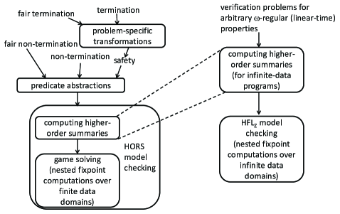
Figure 10: Comparison between HORS- and HFL-based approaches. In the HORS-based approaches (shown on the lefthand side), there are actually some feedback loops (due to counterexample-guided abstraction refinement, etc.), which are omitted. The right hand side shows the approach based on the reduction in Section 7. In the reductions in Section 5 and 6, the first phase is optimized for degenerate cases.

As shown on the righthand side of Figure 10, in our new HFL-based approach, we have extended the first phase of HORS model checking – the computation of higher-order procedure summaries – to deal with infinite data programs, and moved it up front; we then formalized the remaining problems as HFL model checking problems. That can be viewed as the essence of the reduction in Section 7, and the reductions in Sections 5 and 6 are those for degenerate cases. Advantages of the new approach include: (i) necessary information on infinite data is available in the second phase of least/greatest computations (cf. the discussion above on the HORS-based approach), and (ii) various verification problems boil down to the issue of how to prove least/greatest fixpoint formulas; thus we can reuse and share the techniques developed for different verification problems. The price to pay is that the first phase (especially a proof of its correctness) is technically more involved, because now we need to deal with infinite-data programs instead of HORS’s (which are essentially finite-data functional programs). That explains long proofs in Appendices (especially Appendix 0.D and 0.E).

References

- [1] Axelsson, R., Lange, M., Somla, R.: The complexity of model checking higher-order fixpoint logic. Logical Methods in Computer Science 3(2) (2007)
- [2] Bjørner, N., Gurfinkel, A., McMillan, K.L., Rybalchenko, A.: Horn clause solvers for program verification. In: Fields of Logic and Computation II - Essays Dedicated to Yuri Gurevich on the Occasion of His 75th Birthday. LNCS, vol. 9300, pp. 24–51. Springer (2015)
- [3] Bjørner, N., McMillan, K.L., Rybalchenko, A.: Program verification as satisfiability modulo theories. In: SMT 2012. EPiC Series in Computing, vol. 20, pp. 3–11. EasyChair (2012)
- [4] Bjørner, N., McMillan, K.L., Rybalchenko, A.: Higher-order program verification as satisfiability modulo theories with algebraic data-types. CoRR abs/1306.5264 (2013)
- [5] Blass, A., Gurevich, Y.: Existential fixed-point logic. In: Computation Theory and Logic, In Memory of Dieter Rödding. LNCS, vol. 270, pp. 20–36. Springer (1987)
- [6] Blume, M., Acar, U.A., Chae, W.: Exception handlers as extensible cases. In: Proceedings of APLAS 2008. LNCS, vol. 5356, pp. 273–289. Springer (2008)
- [7] Burn, T.C., Ong, C.L., Ramsay, S.J.: Higher-order constrained horn clauses for verification. PACMPL 2(POPL), 11:1–11:28 (2018)
- [8] Carayol, A., Serre, O.: Collapsible pushdown automata and labeled recursion schemes: Equivalence, safety and effective selection. In: LICS 2012. pp. 165–174. IEEE (2012)
- [9] Dijkstra, E.W.: Guarded commands, nondeterminacy and formal derivation of programs. Commun. ACM 18(8), 453–457 (1975)
- [10] Filliâtre, J.C., Paskevich, A.: Why3 — where programs meet provers. In: Felleisen, M., Gardner, P. (eds.) Proceedings of ESOP 2013. LNCS, vol. 7792, pp. 125–128. Springer (2013)
- [11] Grädel, E., Thomas, W., Wilke, T. (eds.): Automata, Logics, and Infinite Games: A Guide to Current Research, LNCS, vol. 2500. Springer (2002)
- [12] Grellois, C., Melliès, P.: Relational semantics of linear logic and higher-order model checking. In: Proceedings of CSL 2015. LIPIcs, vol. 41, pp. 260–276 (2015)
- [13] Haddad, A.: Model checking and functional program transformations. In: Proceedings of FSTTCS 2013. LIPIcs, vol. 24, pp. 115–126 (2013)
- [14] Hesselink, W.H.: Predicate-transformer semantics of general recursion. Acta Inf. 26(4), 309–332 (1989)
- [15] Hofmann, M., Chen, W.: Abstract interpretation from Büchi automata. In: Proceedings of CSL-LICS ’14. pp. 51:1–51:10. ACM (2014)
- [16] Igarashi, A., Kobayashi, N.: Resource usage analysis. ACM Trans. Prog. Lang. Syst. 27(2), 264–313 (2005)
- [17] Jurdzinski, M.: Small progress measures for solving parity games. In: Proceeding of STACS 2000. LNCS, vol. 1770, pp. 290–301. Springer (2000)
- [18] Knapik, T., Niwinski, D., Urzyczyn, P.: Higher-order pushdown trees are easy. In: FoSSaCS 2002. LNCS, vol. 2303, pp. 205–222. Springer (2002)
- [19] Kobayashi, N.: Types and higher-order recursion schemes for verification of higher-order programs. In: Proceedings of POPL. pp. 416–428. ACM Press (2009)
- [20] Kobayashi, N.: Model checking higher-order programs. Journal of the ACM 60(3) (2013)
- [21] Kobayashi, N., Lozes, É., Bruse, F.: On the relationship between higher-order recursion schemes and higher-order fixpoint logic. In: Proceedings of POPL 2017. pp. 246–259 (2017)
- [22] Kobayashi, N., Matsuda, K., Shinohara, A., Yaguchi, K.: Functional programs as compressed data. Higher-Order and Symbolic Computation (2013)
- [23] Kobayashi, N., Ong, C.H.L.: A type system equivalent to the modal mu-calculus model checking of higher-order recursion schemes. In: Proceedings of LICS 2009. pp. 179–188 (2009)
- [24] Kobayashi, N., Ong, C.H.L.: A type system equivalent to the modal mu-calculus model checking of higher-order recursion schemes. http://www-kb.is.s.u-tokyo.ac.jp/~koba/tmp/lics09-full.pdf. A longer version of [23] (2012)
- [25] Kobayashi, N., Sato, R., Unno, H.: Predicate abstraction and CEGAR for higher-order model checking. In: Proc. of PLDI. pp. 222–233. ACM Press (2011)
- [26] Koskinen, E., Terauchi, T.: Local temporal reasoning. In: Proceedings of CSL-LICS ’14. pp. 59:1–59:10. ACM (2014)
- [27] Kozen, D.: Results on the propositional -calculus. Theor. Comput. Sci. 27, 333–354 (1983)
- [28] Kuwahara, T., Sato, R., Unno, H., Kobayashi, N.: Predicate abstraction and CEGAR for disproving termination of higher-order functional programs. In: Proceedings of CAV 2015. LNCS, vol. 9207, pp. 287–303. Springer (2015)
- [29] Kuwahara, T., Terauchi, T., Unno, H., Kobayashi, N.: Automatic termination verification for higher-order functional programs. In: Proceedings of ESOP 2014. Lecture Notes in Computer Science, vol. 8410, pp. 392–411. Springer (2014)
- [30] Lange, M., Lozes, É., Guzmán, M.V.: Model-checking process equivalences. Theor. Comput. Sci. 560, 326–347 (2014)
- [31] Ledesma-Garza, R., Rybalchenko, A.: Binary reachability analysis of higher order functional programs. In: SAS 2012. LNCS, vol. 7460, pp. 388–404. Springer (2012)
- [32] Lozes, É.: A type-directed negation elimination. In: Proceedings FICS 2015. EPTCS, vol. 191, pp. 132–142 (2015)
- [33] Murase, A., Terauchi, T., Kobayashi, N., Sato, R., Unno, H.: Temporal verification of higher-order functional programs. In: Proceedings of POPL 2016. pp. 57–68 (2016)
- [34] Ong, C.H.L.: On model-checking trees generated by higher-order recursion schemes. In: LICS 2006. pp. 81–90. IEEE Computer Society Press (2006)
- [35] Ong, C.H.L., Ramsay, S.: Verifying higher-order programs with pattern-matching algebraic data types. In: Proceedings of POPL. pp. 587–598. ACM Press (2011)
- [36] Rondon, P.M., Kawaguchi, M., Jhala, R.: Liquid types. In: PLDI 2008. pp. 159–169 (2008)
- [37] Salvati, S., Walukiewicz, I.: Krivine machines and higher-order schemes. Information and Computation 239(Supplement C), 340 – 355 (2014), http://www.sciencedirect.com/science/article/pii/S0890540114000984
- [38] Sangiorgi, D.: Introduction to Bisimulation and Coinduction. Cambridge University Press (2012)
- [39] Skalka, C., Smith, S.F., Horn, D.V.: Types and trace effects of higher order programs. J. Funct. Program. 18(2), 179–249 (2008)
- [40] Terauchi, T.: Dependent types from counterexamples. In: Proceedings of POPL. pp. 119–130. ACM (2010)
- [41] Tobita, Y., Tsukada, T., Kobayashi, N.: Exact flow analysis by higher-order model checking. In: Proceedings of FLOPS 2012. LNCS, vol. 7294, pp. 275–289. Springer (2012)
- [42] Tsukada, T., Ong, C.L.: Compositional higher-order model checking via -regular games over böhm trees. In: Proceedings of CSL-LICS ’14. pp. 78:1–78:10. ACM (2014)
- [43] Unno, H., Kobayashi, N.: Dependent type inference with interpolants. In: PPDP 2009. pp. 277–288. ACM (2009)
- [44] Unno, H., Satake, Y., Terauchi, T.: Relatively complete refinement type system for verification of higher-order non-deterministic programs. PACMPL 2(POPL), 12:1–12:29 (2018)
- [45] Unno, H., Terauchi, T., Kobayashi, N.: Automating relatively complete verification of higher-order functional programs. In: POPL 2013. pp. 75–86. ACM (2013)
- [46] Viswanathan, M., Viswanathan, R.: A higher order modal fixed point logic. In: CONCUR. Lecture Notes in Computer Science, vol. 3170, pp. 512–528. Springer (2004)
- [47] Watanabe, K., Sato, R., Tsukada, T., Kobayashi, N.: Automatically disproving fair termination of higher-order functional programs. In: Proceedings of ICFP 2016. pp. 243–255. ACM (2016)
- [48] Winskel, G.: The Formal Semantics of Programming Languages: An Introduction. The MIT Press (1993)
- [49] Winskel, G.: Prime algebraicity. Theor. Comput. Sci. 410(41), 4160–4168 (2009)
- [50] Zhu, H., Nori, A.V., Jagannathan, S.: Learning refinement types. In: Proceedings of ICFP 2015. pp. 400–411. ACM (2015)