Performance of Complex Langevin Simulation in 0+1 dim. massive Thirring model at finite density
Abstract
Statistical sampling with the complex Langevin (CL) equation is applied to (0+1)-dimensional Thirring model, and its uniform-field variant, at finite fermion chemical potential . The CL simulation reproduces a crossover behavior which is similar to but actually deviating from the exact solution in the transition region, where we confirm that the CL simulation becomes susceptible to the drift singularities, i.e., zeros of the fermion determinant. In order to simulate the transition region with the CL method correctly, we examine two approaches, a reweighting method and a model deformation, in both of which a single thimble with an attractive fixed point practically covers the integration domain and the CL sampling avoids the determinant zeros. It turns out that these methods can reproduce the correct crossover behavior of the original model with using reference ensembles in the complexified space. However, they need evaluation of the reweighting factor, which scales with the system size exponentially. We discuss feasibility of applying these methods to the Thirring model and to more realistic theories.
1 Introduction
Simulating a fermion system at finite chemical potentials often leads to the notorious sign problem with a complex action in the path-integral formalism. Study of QCD phase diagram at finite densities is one of the most challenging subjects of this category. Recently, among other extensive attemptsdeForcrand:2010ys , two approaches which involve field complexification have been studied as a promising direction to the solution of the problem. Application of the Langevin equation to a complex action problem is a classic idea Parisi:1984cs ; Klauder:1983zm ; Klauder:1983sp , and has been attracting renewed attention with recent progress Aarts:2008rr ; Aarts:2008wh ; Aarts:2009dg ; Aarts:2009uq ; Aarts:2010aq ; Aarts:2010gr ; Aarts:2011ax ; Aarts:2011sf ; Aarts:2011zn ; Aarts:2012ft ; Aarts:2013uza ; Makino:2015ooa made in the last decade including exploratory applications to QCD at finite density in Seiler:2012wz ; Sexty:2013ica ; Aarts:2014bwa ; Aarts:2014kja ; Fodor:2015doa , also in Nagata:2016mmh (see Aarts:2013uxa ; Aarts:2014fsa ; Seiler:2017wvd for review). Generalization of the steepest-descent-path idea for oscillatory integrals to the multi-dimensional cases is called now the Lefschetz-thimble approach Cristoforetti:2012su ; Cristoforetti:2013wha ; Fujii:2013sra and has been applied to simple bosonic theories Cristoforetti:2013wha ; Fujii:2013sra ; Cristoforetti:2014gsa ; Tanizaki:2014xba ; Tanizaki:2014tua ; Tanizaki:2015pua ; Alexandru:2016san as well as fermionic theories Mukherjee:2014hsa ; Kanazawa:2014qma ; DiRenzo:2015foa ; Tanizaki:2015rda ; Fujii:2015bua ; Fujii:2015vha ; Alexandru:2015xva ; Alexandru:2015sua ; Alexandru:2016ejd . Furthermore several remarks are found in Aarts:2013fpa ; Aarts:2014nxa ; Fukushima:2015qza ; Nishimura:2017vav in conjunction with the two approaches.
Long-time evolution of the Langevin equation of real action
| (1) |
with a stochastic noise is a standard method to generate the equilibrium ensemble of configurations , which is shown by the spectral analysis of the associated Fokker-Planck operator. Apparently, the Langevin evolution can be applied to a complex action system , once the configuration space is complexified: , which results in the complex Langevin (CL) equation. One can solve CLE in practice by applying adaptive stepsize in the Langevin time to suppress numerical instability of the evolution trajectories Aarts:2009dg .
It has been recognized, however, that the resultant distribution in the complexified space converges to an incorrect solution in some cases, including fermionic systems at finite density SanoLattice2011 ; Pawlowski:2013pje ; Pawlowski:2013gag ; Mollgaard:2013qra ; Mollgaard:2014mga ; Hayata:2015lzj . Correctness of the CL method is argued relying on the holomorphic property of the associated Fokker-Planck equation with repeated use of integration by parts, with requiring the distribution localized in imaginary directions Aarts:2009uq ; Aarts:2011sf ; Aarts:2013uza . But the fermion determinant gives rise to a meromorphic drift force, and the condition for correctness of the method is revisited in Refs. Nishimura:2015pba ; Nagata:2015uga ; Nagata:2016vkn ; Aarts:2017vrv , where subtleties with the meromorphic drift term is carefully studied. It is pointed out that the singularities of the drift force give additional surface-term contribution in the integration by parts, and also that they prevent us from taking the continuum limit of the discretized CL equation, depending of the support of the CL sample distribution. It is claimed in Ref. Nagata:2016vkn that CL method gives the correct results if the distribution is suppressed at large drift magnitude exponentially, for large , or stronger.
In this work we examine statistical simulations with the CL equation applied to the (0+1) dimensional Thirring model, and its uniform-field variant, at finite chemical potential Pawlowski:2013pje ; Pawlowski:2013gag ; Pawlowski:2014ada ; Fujii:2015bua . This model is analytically solvable on a finite lattice, showing a smooth crossover with increasing . It has been used as a good benchmark for testing new methods for the sign problem in a fermionic system Pawlowski:2013pje ; Pawlowski:2014ada ; Fujii:2015bua ; Fujii:2015vha ; Alexandru:2015xva . The CL simulations are performed in (0+1) dimensional Thirring model and the results are compared with the analytic results Pawlowski:2013pje ; Fujii:2015bua , and the consistency condition are examinedPawlowski:2013pje . It has been known that CL simulation is successful at small and large outside the crossover, but converges to an incorrect solution in between.
Here we confirm numerically that for in the crossover region the CL simulations of the model becomes susceptible to the singularities of the drift term and the ensemble distribution is only power-suppressed in the vicinities of the determinant zeros, which makes the method unjustifiable thereNagata:2016vkn . From the structure of the drift flow field of the model, it seems inevitable that the CL sampling hits the vicinity of the drift singularities (fermion determinant zeros) for in the crossover region. At small or large , where CL method is successful, the determinant zeros locate outside the support of the CL ensemble.
In view of the thimble (steepest descent path) integration, the abrupt crossover behavior is resulted from the contributions of the multi thimbles connected via the determinant zerosTanizaki:2015rda ; Fujii:2015bua ; Fujii:2015vha . The destructive interference between multi-thimble contributions poses the global sign problem in numerical evaluation. In contrast, at zero or large , a single thimble practically covers the integration domain. In this latter case, the CL sampling around the thimble does not hit the determinant zeros.
Several attempts are made so far in order to extend the applicability of CL simulations to the crossover region. One is the reweighting method: Observables in the crossover region are computed by reweighting with the CL ensembles generated at a reference point within the (multi-) parameter space where the CL method is valid Bloch:2016jwt ; Bloch:2017ods ; Bloch:2017sfg , at the cost of the so-called reweighting factor. Deformation of the models is proposed in Tsutsui:2015tua ; Doi:2017gmk , where the fermion determinant is modified so that the determinant zeros become irrelevant in the CL sampling, and observables of the original model are re-expressed exactly in terms of those of the deformed models. Another model-deformation method is studied in Ito:2016efb with introduction of an auxiliary parameter into the fermion determinant to study the spontaneous symmetry breaking. The CL method is applied to a fermionic model within the applicable parameter region, and then the zero limit of the parameter is taken by extrapolation. The gauge cooling method is extended in Nagata:2016alq for avoiding the artificial singular drift problem in a random matrix model.
In this work, we examine the reweighting methodBloch:2017ods and model-deformation methodTsutsui:2015tua ; Doi:2017gmk . The latter may be regarded as a kind of reweighting method, for it needs evaluation of the reweighting factor, too, as seen in Eq. (4.1) below. In reweighting we use the CL ensembles generated with zero or large , for which the ensemble supports have no overlap with the vicinity of the zeros and also the corresponding thimble structure becomes simple. The reweighting method can reproduce the correct crossover behavior (for a small system size), which enforces the correctness of the CL ensembles generated outside the crossover region. Then we study the efficiency of the reweighting method by changing the system size. For deformation method, we find a subtlety in dealing with the pole of the fermion observables such as number and scalar densities. We will comment on this point, in addition to the efficiency of the method.
This paper is organized as follows: In the next section we present the definition of the model and its uniform-field variant, and perform CL simulations for them. We then analyze the success and failure of CL simulations by inspecting the ensemble distributions on the complex plane in relation to the zeros, critical points, and thimble structure in some detail, and make histograms of the drift force to test the criterion for the validity of CL method. We end Sec. 2 with a brief summary. In Sec. 3 we apply the re-weighting method to simulate the model in the crossover region using zero- and large- reference ensembles. Main focus is the efficiency of the re-weighting w.r.t. the system size toward larger systems. In Sec. 4 we examine the deformation method, where we encounter a difficulty due to the poles in the observable and/or numerical efficiency in this approach. Sec. 5 is devoted to Summary. Appendix A present analytic expressions for the determinant zeros in the deformed model.
2 Model
2.1 Thirring model in (0+1) dimensions
We deal with the lattice Thirring model with a single staggered ferimon in (0+1) dimensions at finite chemical potential . After unfolding the vector-type four-point interaction, we can write the partition function as a path integral over a compact auxiliary filed Pawlowski:2013pje ; Pawlowski:2013gag ; Pawlowski:2014ada ; Fujii:2015bua :
| (2) |
with the bosonic action and the fermion determinant 111 Note that we have omitted an irrelevant factor of in for notational simplicity.
| (3) |
where is the temporal lattice size, the inverse coupling constant, the fermion mass term. We have set the lattice unit and all the dimensionful quantities are measured in the lattice unit hereafter. We notice here that depends on the field configuration only through the sum . The sign problem arises from the complex determinant at nonzero in this model.
The analytic expression for is known as
| (4) |
where are the modified Bessel function of the first kind. The fermion number density and scalar density are obtained, respectively, as
| (5) |
with
| (6) |
and
| (7) |
with
| (8) |
At zero chemical potential , the fermion number density vanishes and the scalar density is nonzero . These densities show crossover-transition behavior as the chemical potential is increased at fixed , or temperature . In the zero temperature limit , the crossover behavior changes to a first-order transition at a critical value of .
2.2 Uniform-field model
For studying analytic properties of the CL sampling in the complexified configuration space, it is instructive to introduce a single-variable model which can be deduced from the (0+1) dimensional Thirring model by setting uniform-field condition, for all . Then the bosonic action reduces to and the “determinant” term becomes
| (9) |
The partition function of this model is given as
| (10) |
The fermion number density and scalar density are defined in the same way as before:
| (11) |
with
| (12) |
and
| (13) |
with
| (14) |
The parameter is a remnant of the lattice size, with which we can study the system size dependence in this uniform-field model. We use this model for examining the analytic properties of the CL sampling and the severity of the sign problem.
2.3 CL simulation
For the Thirring model in (0+1) dimensions, the CL evolution in the Langevin time with discrete step , is written collectively for the complexified variables () as
| (15) |
with the drift force
| (16) |
and with the real stochastic force whose average satisfies and . The sum becomes complex-valued, too. For the uniform-field model we have a single equation with the same structure as above, where the drift force reads
| (17) |
Notice that the zeros of the determinant give rise to singularities of the drift force in both cases.
Expectation values of observables are computed with the ensemble distribution sampled along with a CL trajectory as
| (18) |
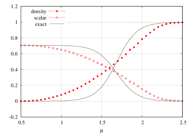
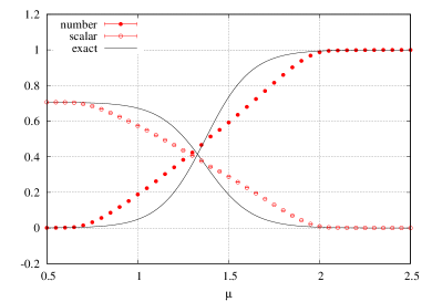
(a) (b)
We have performed the CL simulation for these models at finite . We set the model parameters as , , , and we choose for the Langevin time step. After steps for thermalization, we evolve the equation by steps with sampling the configurations in every steps. When the drift magnitude becomes large such that , we evolve the equation with a smaller step size to keep till is achieved. Since the model is periodic in , we restricted in the simulations.
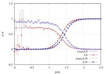
The simulation results for the fermion number density and scalar condensate in the Thirring model are plotted as a function of in Fig. 1 (a). The exact results (solid curves) clearly show smooth crossover behavior in the region of . In contrast, the CL results for and deviate from the exact ones, showing milder dependence on around the crossover region. They agree with the exact results for small and large values of . A similar trend is also seen in the CL result for the uniform-field model as shown in Fig. 1 (b); the exact solution shows crossover transition in the region of , while the CL result behaves almost linearly with increasing in the corresponding region.
2.4 CL ensembles, determinant zeros and thimbles
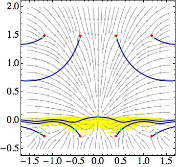
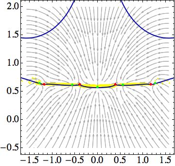
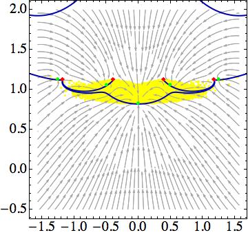
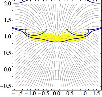
It has been noticed for some time that the CL method fails in crossover regions for simple fermionic models with singular drift terms, such as the chiral random matrix model, the models with modified Rayleigh distributions, Hubbard model, etc., in addition to the (0+1) dimensional Thirring model SanoLattice2011 ; Pawlowski:2013pje ; Pawlowski:2013gag ; Mollgaard:2013qra ; Mollgaard:2014mga ; Hayata:2015lzj . In order to understand the situation clearly, we present in Fig. 2 the scatter plots of the CL samples in the uniform field model for and with . We collected samples and show them with yellow dots in the complex plane. In the same figure, we also display the drift flow field (17) with gray arrows, and the zeros of the determinant in red diamonds, where the drift become singular. Green circles denote the fixed points of the drift force field.
Blue curves are the steepest descent paths for , or the thimbles in Lefschetz theory. The thimbles are defined by the union of integral curves of the anti-holomorphic flow
| (19) |
with the boundary condition, . It is known that a set of thimbles becomes equivalent to the original integration contour:
| (20) |
One important property of the anti-holomorphic flow is that is monotonically increasing with kept constant along the flow, especially on a thimble. This property motivated us to perform Monte Carlo simulations on thimblesCristoforetti:2012su ; Cristoforetti:2013wha ; Fujii:2013sra .
This anti-holomorphic flow field is obtained from the drift force field by flipping the sign of the real component. Under this transformation, zero points and critical points , which are saddle points and attractive (or repelling) points in CL method, respectively become attractive points 222 Since we assume that is bounded below, we don’t have repelling points here. and saddle points in Lefschetz theory. Since the total set of thimbles form a skeleton graph without loops, there must be an associated critical point for each zero point , which provides an endpoint for a thimble .
In Fig. 2, we first notice that the critical point on the imaginary axis is an attractive point of the drift force field for all the values of studied here, and it is always included in the CL ensemble. Indeed, thimble is always the most dominating one in the thimble integration in this model. At (Fig. 2 (a)), the distribution of the CL samples is elongated along the original integration contour, the real axis , having small extent in the imaginary direction. It also has a good overlap with the thimble emerging from the critical point . We note that the distribution apparently has no overlap with the vicinity of any .

(a) (b)
(c)
(d) (e)
At a slightly larger chemical potential (Fig. 2 (b)), however, the distribution gets expanded in the imaginary direction to have an overlap with the vicinity of some zeros of the determinant. This situation is understood as follows: With increasing , the zeros move upward together with their associated critical points 333 See Appendix A for the explicit expressions for ’s. , and a reconnection of the thimbles (the Stokes phenomenon) occurs between and 0.6. At the thimble terminates at the two zeros closest to the origin, and the integration contour now consists of multi thimbles. A change of the thimble structure must accompany a change of the drift flow pattern, because the anti-holomorphic flow defining the thimbles is obtained just by flipping the sign of the real component of the drift flow 17 of CL method.
We show a representative configuration of a CL ensemble, drift field and thimbles at in Fig. 2 (c), where the thimbles are connected with each other at ’s, and the CL samples are distributed closely to the thimbles 444 It is known that there is other models where a critical point of a relevant thimble becomes repulsive and not sampled in the CL sampling. . Until (Fig. 2 (d)), the CL sampling includes the vicinities of the zeros, and exactly in this region of , the CL results converge to the incorrect solution. Above this value of the chemical potential, as is seen in Fig. 2 (e), the CL samples are distributed away from any zeros and localized around the single thimble covering practically the whole integration contour. In this case, the CL simulation gives the the correct result (see Fig. 1 (b)).
Importance of multi-thimble contributions in the transition region is emphasized in Refs. Tanizaki:2015rda ; Fujii:2015bua ; each thimble has a complex phase of , and destructive interference among multi-thimble contributions is crucial for realizing the Silver-Blaze phenomenonCohen:2003kd , i.e., no response of the system to below a certain critical value at zero temperature.
Because the thimbles in the set which is equivalent to the original integration contour are connected at the determinant zeros and because the CL samples are well localized around the thimbles in this model, it seems almost inevitable that the CL samples the neighborhoods of the drift singularities (determinant zeros). In Fig. 2 (c), the critical points and zero points are aligned almost in a straight-line parallel to the real axis, and then these critical points become attractive nodes and these zeros are saddle points in the drift flow field. We also notice that in the thimble integration one needs to include correctly the complex phases from and the Jacobian in the change of the variables, while in the CL method observables are computed as a simple average of the samples distributed around the thimbles in the complex plane without any additional phase factors.
Outside the crossover region, the integration contour is dominated solely by a single thimble, and relative phases among the thimbles become irrelevant. In the CL approach, this implies that the vicinities of the determinant zeros are not sampled so that the simulations give the correct results.
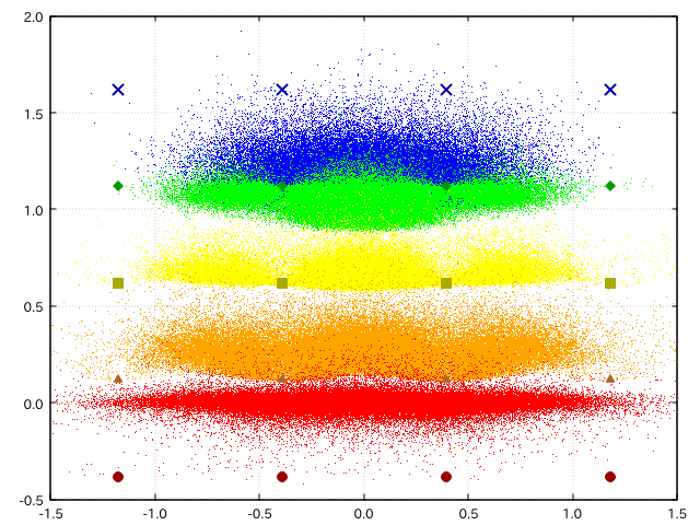
In Fig. 3, we show a scatter plot of the (0+1) dimensional model in complex space, for and with , , and in the complex plane. The zero manifold, where , projected on this plane becomes a set of points, which we denote with circles, triangles, squares, diamonds, and crosses for respective values of in Fig. 3.
We confirm that the CL ensembles overlap with the neighborhoods of the determinant zeros for in the crossover region (). We also note that the samples are scattered wider in imaginary direction than in the uniform-field model.
(a) (b)

(a) (b)
2.5 Histogram of drift force
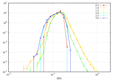
Recently authors of Ref. Nagata:2016vkn claimed that an exponential fall-off of the probability of the drift term at large magnitude is the necessary and sufficient condition for the correctness of the CL results. Indeed, the histogram of is very helpful to quantify the contributions from the vicinities of the zeros in the CL simulations.
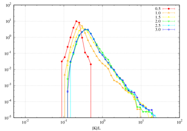
We make histograms of the drift force of the uniform-field model with , and for and in Fig. 4 (a) by binning the drift magnitude as (we chose here and integer). Outside the crossover region, and , we find that the histograms fall off very sharply and become vacant at large . But it develops a power-law tail for in the crossover region, which clearly show the fact that the CL sampling hits the vicinities of the determinant zeros. This result is consistent with the argument of Ref. Nagata:2016vkn .
In Fig. 4 (b), we make histograms of of the (0+1) dimensional Thirring model with =8, and for , 1.0, 1.5, 2.0, 2.5, 3.0. At small , for which the CL simulation is successful, the histogram is well localized around . But we find that a power-law-like distribution of appears for , which may be caused by the singularities of the force at the determinant zeros. From Fig. 1 (a), however, the value is well outside the crossover region and the CL simulation successfully reproduce the correct result. Moreover, from Fig. 3 the vicininities of the zeros are little sampled at this value of , in spite of the power-low tail appearing in the histogram. .
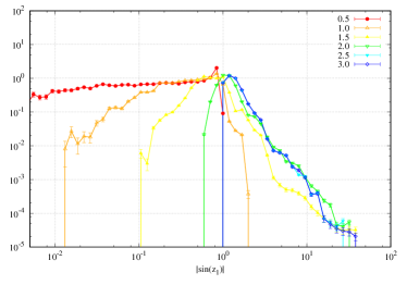
To measure the contributions from the vicinities of the drift singularities, we make histograms of in Fig. 5 (a). We find that the histogram is empty at large for and 3.0, i.e., for outside the crossover region, while the power-law tail appears for in the crossover. It is concluded, therefore, that the power-law-tail contribution from the neighborhoods of the drift singularities exists only in the crossover region to make the CL method dubious there.
Then the power-law tail at large in the histogram Fig. 4 (a) for large must come from the first term in the drift force, (16). This is indeed the case as can be confirmed by looking at the histogram of , for example, in Fig. 5 (b). We see that the probability of large develops as increases.
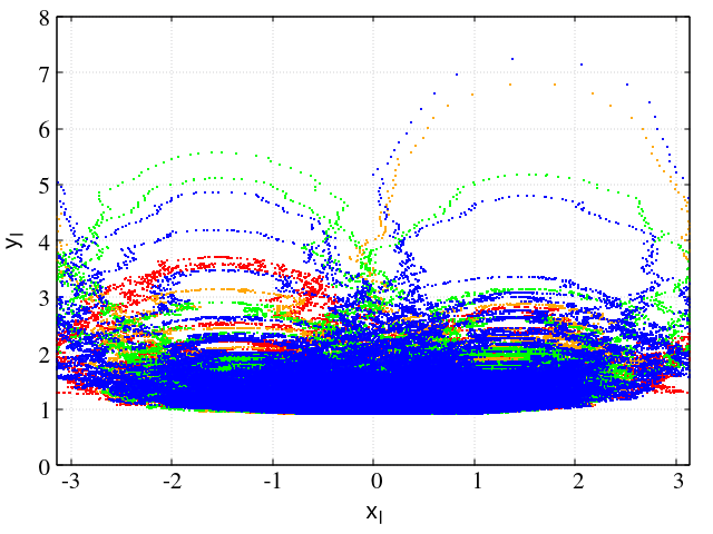
This power-law tail of the -distribution for large (=3) appears by fluctuations of () in imaginary direction. In the (0+1) dimensional model, with localized around the critical point (Fig. 3), a component can first fluctuate in real direction to the region with . Then a trajectory rides on a drift flow to imaginary direction, which is caused by term in the flow, (16), and the trajectory makes an excursion in the imaginary direction which then comes back to the region near (See Fig. 6). We have confirmed that the histogram of integrated over other variables is consistent with an exponentially decaying distribution with for . When plotted with respect to , the histogram decays with power law in large region, which is seen in Fig. 5 (b).
2.6 Short summary
We have seen that the CL simulation converges to an incorrect solution within the crossover region of the model, where CL samples the neighborhoods of the determinant zeros, , as seen in the histograms of the drift force and also in the scatter plots. This is the very situation where CL method becomes dubious as is argued in Refs. Nagata:2016vkn ; Aarts:2017vrv . We have also seen that it is almost inevitable for CL simulations to sample the vicinities of these zeros ’s from the observation of the drift flow pattern in the crossover region, where contributions from multi-thimble connected with each other via these zeros become important in the thimble integration.
Outside the crossover region, on the other hand, the CL simulation successfully reproduces the correct solution. In this region, the thimble structure in the complexified configuration space is so simple that a single thimble becomes practically equivalent to the original integration domain, and the CL ensemble is well localized around this single thimble without sampling the vicinity of any determinant zeros ’s.
In order to apply the CL simulation in the crossover region, therefore, we need methods which avoid sampling the vicinity of ’s. One possible approach to overcome this situation is the so-called re-weighting method, in which one evaluates the observables in the crossover region by using the ensemble generated in other parameter region where the CL method gives the correct resultsBloch:2017ods . Another approach is to express the observables with a deformed (or modified) model for which the CL simulation is successful without sampling the vicinity of its zerosTsutsui:2015tua .
We examine these two approaches one by one in the next two sections.
3 Reweighting method at finite
In order to compute the observables correctly in the crossover region, one can try the reweighting method with CL ensembles in the parameter space () where CL method works well Bloch:2017ods . We have observed that the CL simulation is successful for outside the crossover region, where a single thimble practically covers the original integration contour and the CL ensembles are distributed along this thimble. Based on this observation, we study here the reweighting method with the CL ensembles generated at a large reference chemical potential, which we call .
In this approach, we recast the expectation value of an observable as
| (21) |
where the subscript indicates that the expectation value is evaluated with the weight and similarly for . In usual reweighting, one introduces a real weight function so that one can perform Monte Carlo sampling. For our model we can choose or as the weight function. But in the context of CL simulations, one may take the system with large chemical potential outside the crossover region as the reference system, and perform the CL simulation to evaluate the observables using Eq. (21). The reweighting method with the CL method is expected to work as long as is outside the crossover region but the reference ensembles still have sufficient overlap with the physical one, as discussed below.
3.1 Reweighting factor
Severity of the sign problem in this approach appears in the evaluation of the reweighting factor with the reference ensemble
| (22) |
In the second line, we have changed the integration contour from the real axis to a set of the thimbles for the function , because the integrands are holomorphic. In the CL simulation with large , the ensembles are localized along a single thimble which covers the dominant part of the integration contour in the complex plane. This suggests that the integration with the CL method is closely related to the integration along the thimble , i.e., the second expression of eq. (22).
It is noteworthy that the reweighting factor is expressed with the average phase fluctuation factor Eq. (24) as
| (23) |
where the average phase fluactuation is defined as the integral along the thimbles:
| (24) |
This clearly shows that the average phase factor (24) is a good measure of the severity of the sign problem in evaluation of the reweighting factor. Note that the denominator of Eq. (24) is now an integral of a non-holomorphic function, and that the average phase factor (24) depends on the choice of the integration path. By setting , the integration path reduces to the real axis and the expression (24) coincides with the usual phase factor
| (25) |
because is real positive there.
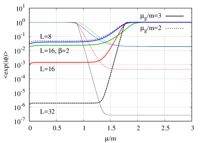
We plot in Fig. 7 the averaged phase factors, and as a function with fixed (dashed) and 3 (solid) for and in the uniform-field model. The phase average with is unity at small and starts to decrease around , which is close to the threshold value for the failure of the simple CL simulation. It continues to decrease until around and becomes constant for larger . But the value of the phase average at large is suppressed exponentially in ; it becomes as small as for at large , and in order to get signal at large , one needs at least samples in statistical sampling. For the number of required samples is likely to become more than . For it is more than .
In contrast, the phase average evaluated along the thimbles is almost unity on the large side. This can be understood by noting the fact that the location of the dominant thimble becomes less sensitive to the value of when is set to a larger value above the crossover region. One can show that for large the critical point appears at on the imaginary axis, independently of . Then the thimbles for large and locate very close to each other, on which the integrands are real positive up to the Jacobian, and therefore the phase factor in eq. (24) becomes close to unity.555In CL simulations the integration measure is replaced with the ensemble average, and the ensembles generated by the CL evolution with these and are closely overlapped with each other. At small , on the other hand, the phase average becomes small because the integrand of is now complex-valued and very oscillatory along the dominant thimble of in the complex plane. We notice here that the situation here is quite opposite to the reweighting at : one needs large ensembles exponentially in the size , to get signals at small , while the simulations at large becomes easier.
We also show in Fig. 7 the reweighting factor for but with , intending one step toward the continuum limit from and . In this change of parameters, the reweighting factors take the similar values to those in the case with and .


3.2 Uniform-field model
Now we apply the reweighting method to the uniform-field model with the parameters with choosing the reference chemical potential to and . As seen in Fig. 1, the value is well above the crossover region, where CL method gives the correct results.
For this parameter set, the phase average or becomes as small as of order , which implies that we will lose numerical accuracy by this factor in the reweighting. Thus, in order to detect significant signals, we collected samples in the CL simulations of steps with the step size by making measurements every 100 interval steps.
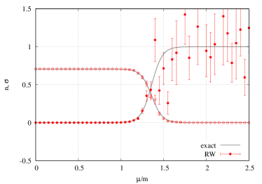
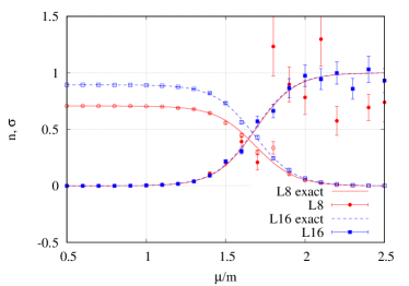
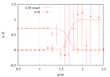
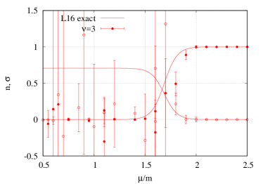
In Fig. 8, results of reweighting at (left panel) and (right panel) for are presented with red circles. The bars indicate the statistical uncertainties assuming that the samples with interval are independent. We find that the reweighting method reproduces the correct results reasonably for the fermion number and scalar densities. If we look closer in the crossover region , we find that the reweighting at works slightly better than the reweighting at . This can be understood from the smallness of the phase factors, and , presented in Fig. 7.
The results of the same model on the finer lattice (, ) at the one step toward the continuum limit, are also shown with squares in Fig. 8. We recognize here that the reweighting method works with similar quality between and .
We perform the same simulations for lower-temperature case, , and show the result in Fig. 9. The statistical uncertainties become substantially larger in this case than in the previous case. This is again consistent with the smallness of the phase average shown in Fig. 7. The ensemble size is still insufficient to assure a good accuracy of the numerical results. The size required for obtaining the significant numerical accuracy will increase exponentially with . We notice here that in the crossover region of the reweighting results at have smaller uncertainty bars than those at in Fig. 9.
3.3 Thirring model in (0+1) dimensions
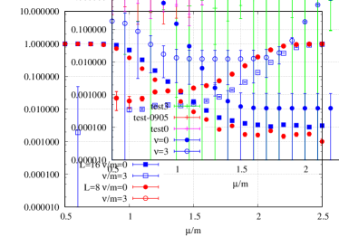
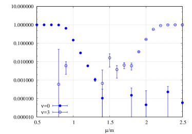
We collected samples with 200 interval steps (, ) to draw the figures in this subsection. First we show in Fig. 10 the expectation value of the phase average, the CL counterpart of Eq. (24). The left panel shows the results for and . We see that the phase average obtained in the phase quench simulation at (filled circles) decreases to about at large . In contrast, the phase average evaluated with the reference parameter (open circles) becomes a few times in the crossover region but even turns to be negative with substantial errors for . On the finer lattice, , the result for the phase average evaluated with ensemble (filled squares) becomes a bit larger in large region, while the phase factor evaluated with ensemble (open squares) takes smaller values in the crossover region, as compared to case. This results suggest that the sample points more than will be required to study these system with the CL simulations, if the statistical uncertainty scales with square root of the sample size.
However, when we decrease the temperature by changing from with fixed, the phase average becomes smaller by one order of magnitude with substantially larger statistical errors, as is shown in the right panel of Fig. 10. We performed CL simulations with and 3 to generate the reference ensembles of size , but after reweighting we did not obtain any significant results in the crossover region. This result suggests that we need to search more efficient reference parameters and in addition to , in order to apply the reweighting method at lower temperature, which we leave for future study.

4 Deformation method
Tsutsui and DoiTsutsui:2015tua proposed a model deformation for a simple fermionic model to avoid the problem of the determinant zeros, by noting an empirical relation between the multi-thimble structure of the model and the failure of the CL simulation. In this section, we examine the deformation method by applying it to the uniform field model.
4.1 Exact expressions
In Ref. Tsutsui:2015tua an extra term is added to the polynomial term of the original model so that the deformed model has a single thimble covering the integration contour and the CL mothod becomes applicable to the model. Then the observables of the original model are expressed exactly in terms of those of the deformed models, by utilizing the following identity 666The second expression is due to S. Shimasaki.:
| (26) |
where denote respectively the expectation values taken with the partition functions,
| (27) |
with certain functions, and . In the present model, we identify , and among many possibilities for we choose here with a reference chemical potential. (Hereafter, we denote the physical chemical potential . The expectation value is taken with the fermion quenched model without and factor. This identity will be beneficial if one can find such that CL simulation produces the correct results for even when it does not work for . Vanishing is the most beneficial case. But there is no general proof for the existence of such a special choice of for a given model.
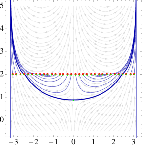
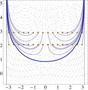
In the uniform-field model, we have seen that CL method gives the correct results for a large , where the thimble structure becomes simple and the original integration contour is practically covered with a single thimble. By choosing the reference chemical potential large, we can make the thimble structure of the deformed model (as well as ) simple for within the range considered here. For we draw the thimble structure of the deformed model with and (left) and 2 (right) in Fig. 13. All the zero points locate well above the real axis in the imaginary direction and the single dominant thimble practically covers the integration domain for in the range considered here (see Appendix A for analytic expressions for the zero points).
The sign problem in this expression remains in the multiplier appearing in Eq. (4.1): Both the integrands in the denominator and numerator become very oscillatory for large . This multiplier is actually the inverse of the reweighting factor as is indicated in the second line of Eq. (4.1).
We evaluate the exact expression (4.1) with CL method for the observables (12) and (14). We notice here, however, that CL simulations may hit the poles of these observables depending on the value of , although the poles of the drift term of the deformed model are avoided by choosing large. The CL simulation will not be justified for such values of in this approach.
Concerning this point, we like to remark that if we adopt also for the number density observable the deformed expressions,
| (28) | ||||
| (29) |
then we find another, but similar identity:
| (30) |
We also have a corresponding identity for with deformed expressions . The expression (II) has two good properties; (i) the pole locations of are the same as those of the drift term, which are avoided in the CL evolution by taking large enough, and (ii) we have analytic expressions for to be compared with the numerical results.
4.2 Numerical results
We present numerical results of the deformation method applied to the uniform-field model for and with . In the simulations we chose here and , and collected the samples with interval steps.
4.2.1 Case (I)

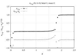


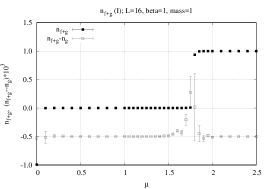

We display the numerical results of the deformation method (I) applied to the uniform field model for in the upper row of Fig. 14, and those for in the lower row. We choose here . For this value of the integration contours practically get covered by the dominant thimbles of , respectively. The left panels show the density obtained by formula (I), and the middle and right panels show the intermediate quantities appearing on RHS of formula (I).
We show in middle panels of Fig. 14 as a function of . The CL results for both and actually show abrupt changes around (and ). We have confirmed that they are almost consistent with the values obtained by integration along the thimbles of . In the thimble integration, these densities make jumps as the poles in the integrand (12) cross the integration contours, but they show abrupt but smooth change here because the CL ensembles extend over the complex plane, not on a line. We also show with an offset the difference there, which has a spike because the abrupt change of each term occurs at different because the CL ensembles for are not identical 777 If we evaluate and by integration along the thimble, the poles of their integrands cross the thimbles at different values of because the thimbles of are slightly different. As a result, the subtracted density shows a spike. In order for (I) to hold, one must choose the same integration contour in each term on RHS so that the pole contributions must cancel out on LHS of Eq. (4.1). .
As shown in left panel of Fig. 14, the numerical result of (I) for reproduces the crossover behavior fairly well except in the regions and , where we see the spike structure. In the CL simulations, a complete cancellation of the abrupt changes in the subtraction term on RHS is impossible to reproduce the exact result. Moreover the poles in the expression of the observable make the correctness of CL simulation very dubious.
In formula (I), the gradual dependence of the exact curve should be reproduced by a delicate combination of and , because is almost flat except for the abrupt changing point of . It is statistically challenging to evaluate accurately the subtraction and the reweighting factor (right panel) for larger size systems. Note the magnification factors and in the plot of the subtracted density for , respectively. The numerical severity is seen clearly in the result for as shown in the lower panels of Fig. 14, where we have much larger statistical errors.
4.2.2 Case (II)


In case (II), expressions for the observables have the poles at the same locations as the drift term, which are avoided in the CL simulation by taking large. Thus the fermion number densities, , will not show any abrupt dependence on , unlike to case (I). We show in Fig. 15 the fermion number density obtained for (upper) and 16 (lower) with and , by using formula (II) and compare it with the exact result [left] and its decomposition [right], (filled circles) and (crosses). In Fig. 15, dependence of numerical result for each term is smooth and very consistent with the exact result within the errors.
However, for the reference value large above the crossover value, both become nearly unity regardless of the value of within the range of our interest (see Eqs. (28) and (29)). After taking subtraction, , we are left with a tiny number as seen in the right panel of Fig. 15. In order to get the fermion number density , we multiply to this density difference the reweighting factor , whose evaluation becomes more difficult at the smaller and the larger . Although formula (II) gives a fair result in the crossover region for , the problem becomes already challenging for , as is seen in Fig. 15.
5 Summary
We have studied applicability of the LC simulation method to the Thirring model in (0+1) dimensions at finite , and its uniform-field variant.
The CL simulations reproduce the exact solution at small and large . However, they deviate from the exact one in the crossover region, where the CL ensemble distribution has an overlap with the neighborhoods of the determinant zeros, where the drift force becomes singular. This observation is consistent with the argument for correctness of the CL simulation, given in Refs. Nagata:2016vkn (see also Aarts:2017vrv ).
We have found that the ensemble distribution localizes around the thimbles in the CL simulations for the Thirring model, in which the critical points of the relevant thimbles behave as attractive points of the drift flow field and the zeros of the determinant become the saddle points of the flow. It seems inevitable in this model that the CL ensemble has an overlap with the determinant zeros whenever the corresponding thimble integration has contributions from multi thimbles connected via these zeros.
In order to extend the applicability of the CL simulation to the crossover region, we have attempted two methods, both of which make the thimble structure of the model simple to cover the integration path with a single thimble in view of the thimble integration. But we have noticed that both methods need the evaluation of the reweighting factor. With the direct reweighting method at large reference chemical potential , we can reproduce the correct crossover behavior of the observables as a function of physical chemical potential . In this sense, one can think of the ensemble generated by CL method physical when CL simulation is successful and can be used for the reweighting. In the deformation method, we also reproduce the correct result but there appears an unphysical structure when the observables have the poles coming from the original determinant zeros. But one can remove this unphysical structure by employing the deformed expressions for the observables in accord with the model.
For a large system size, however, both methods encounter a difficulty in evaluating the reweighting factor; the phase factor average amounts to a small value which scales exponentially with the system size. In the deformation method, we need to evaluate the subtraction of the two expectation values of the similar magnitudes, which gives an additional limitation on the method.
Here we only choose the chemical potential as a reference parameter, but one can consider other reweighting by taking other model parameters, such as the mass or temperature , etc., as reference parameters for the reweighting. We leave the examination of the multi-parameter reweighting method for future work.
The eigenvalue distribution of the fermion operator of the models here in the configuration space complexified by CL method is also intriguing quantity to be studied, as was discussed in Ref. Pawlowski:2013pje ; Splittorff:2014zca ; Mollgaard:2014mga .
Acknowledgement S.K. is very grateful to S. Shimasaki for useful discussions on this work. This work was supported in part by Grants-in-Aid of JSPS, # 16K05313 and 16K05343.
Appendix A Determinant zeros in uniform-field model
We show the zero points of the uniform-field model and those for the deformed model.
First, the analytic structure of the reference system is the same as with a simple replacement of ; the zeros in the uniform-field model, are given asFujii:2015bua
| (31) |
and there appear critical points associated to these zeros as seen in Fig. 2.
In order to understand the thimble structure of the modified model, , let us first find the zeros of . To this end, it is convenient to introduce defined by , in terms of which and with . Then the zero-point condition is recast as
| (32) |
Denoting the ratio , we easily find the zeros as
| (35) |
For the ’s line up in the plane along a straight line parallel to the real axis offset by to the imaginary direction. For they appear with an equal separation along the two straight lines separated by . In both cases the modified model has zeros in total, just as many as the original model. Setting large enough, we can make these zeros (and the associated critical points, too) appear with large imaginary axis in the complex plane. We note, however, that one critical point on the imaginary part remains sitting at (and another critical point on the axis) for large with fixed .
We show the thimble structure of for and 2 with in Fig. 13, for example. One recognizes that the original integration contour on the real axis can be replaced with a set of thimbles which includes the thimble starting at the critical point on the imaginary axis. This thimble gives the most important contribution to the integral. By increasing the value, we can move the critical points associated to the zeros further upward so that the single thimble becomes equivalent to the original integration contour.
References
- (1) P. de Forcrand, “Simulating QCD at finite density,” PoS LAT 2009, 010 (2009) [arXiv:1005.0539 [hep-lat]].
- (2) M. Creosoted et al. [AuroraScience Collaboration], “New approach to the sign problem in quantum field theories: High density QCD on a Lefschetz thimble,” Phys. Rev. D 86, 074506 (2012) [arXiv:1205.3996 [hep-lat]].
- (3) M. Cristoforetti, F. Di Renzo, A. Mukherjee and L. Scorzato, “Monte Carlo simulations on the Lefschetz thimble: Taming the sign problem,” Phys. Rev. D 88, no. 5, 051501 (2013) [arXiv:1303.7204 [hep-lat]].
- (4) H. Fujii, D. Honda, M. Kato, Y. Kikukawa, S. Komatsu and T. Sano, “Hybrid Monte Carlo on Lefschetz thimbles - A study of the residual sign problem,” JHEP 1310, 147 (2013) [arXiv:1309.4371 [hep-lat]].
- (5) M. Cristoforetti, F. Di Renzo, G. Eruzzi, A. Mukherjee, C. Schmidt, L. Scorzato and C. Torrero, Phys. Rev. D 89, no. 11, 114505 (2014) [arXiv:1403.5637 [hep-lat]].
- (6) Y. Tanizaki and T. Koike, “Real-time Feynman path integral with Picard-Lefschetz theory and its applications to quantum tunneling,” Annals Phys. 351, 250 (2014) [arXiv:1406.2386 [math-ph]].
- (7) Y. Tanizaki, Phys. Rev. D 91, no. 3, 036002 (2015) [arXiv:1412.1891 [hep-th]].
- (8) Y. Tanizaki, H. Nishimura and K. Kashiwa, “Evading the sign problem in the mean-field approximation through Lefschetz-thimble path integral,” Phys. Rev. D 91, no. 10, 101701 (2015) [arXiv:1504.02979 [hep-th]].
- (9) A. Alexandru, G. Basar, P. Bedaque, G. W. Ridgway and N. C. Warrington, “Study of symmetry breaking in a relativistic Bose gas using the contraction algorithm,” Phys. Rev. D 94, no. 4, 045017 (2016) doi:10.1103/PhysRevD.94.045017 [arXiv:1606.02742 [hep-lat]].
- (10) A. Alexandru, G. Basar, P. F. Bedaque, S. Vartak and N. C. Warrington, “Monte Carlo Study of Real Time Dynamics on the Lattice,” Phys. Rev. Lett. 117, no. 8, 081602 (2016) doi:10.1103/PhysRevLett.117.081602 [arXiv:1605.08040 [hep-lat]].
- (11) A. Mukherjee and M. Cristoforetti, “Lefschetz thimble Monte Carlo for many-body theories: A Hubbard model study,” Phys. Rev. B 90, no. 3, 035134 (2014) [arXiv:1403.5680 [cond-mat.str-el]].
- (12) T. Kanazawa and Y. Tanizaki, “Structure of Lefschetz thimbles in simple fermionic systems,” JHEP 1503, 044 (2015) [arXiv:1412.2802 [hep-th]].
- (13) F. Di Renzo and G. Eruzzi, “Thimble regularization at work: from toy models to chiral random matrix theories,” Phys. Rev. D 92, no. 8, 085030 (2015) doi:10.1103/PhysRevD.92.085030 [arXiv:1507.03858 [hep-lat]].
- (14) Y. Tanizaki, Y. Hidaka and T. Hayata, “Lefschetz-thimble analysis of the sign problem in one-site fermion model,” New J. Phys. 18 (2016) no.3, 033002 doi:10.1088/1367-2630/18/3/033002 [arXiv:1509.07146 [hep-th]].
- (15) H. Fujii, S. Kamata and Y. Kikukawa, “Lefschetz thimble structure in one-dimensional lattice Thirring model at finite density,” JHEP 1511, 078 (2015) Erratum: [JHEP 1602, 036 (2016)] doi:10.1007/JHEP02(2016)036, 10.1007/JHEP11(2015)078 [arXiv:1509.08176 [hep-lat]].
- (16) H. Fujii, S. Kamata and Y. Kikukawa, “Monte Carlo study of Lefschetz thimble structure in one-dimensional Thirring model at finite density,” JHEP 1512, 125 (2015) Erratum: [JHEP 1609, 172 (2016)] doi:10.1007/JHEP12(2015)125, 10.1007/JHEP09(2016)172 [arXiv:1509.09141 [hep-lat]].
- (17) A. Alexandru, G. Basar and P. Bedaque, “Monte Carlo algorithm for simulating fermions on Lefschetz thimbles,” Phys. Rev. D 93, no. 1, 014504 (2016) doi:10.1103/PhysRevD.93.014504 [arXiv:1510.03258 [hep-lat]].
- (18) A. Alexandru, G. Basar, P. F. Bedaque, G. W. Ridgway and N. C. Warrington, “Sign problem and Monte Carlo calculations beyond Lefschetz thimbles,” JHEP 1605, 053 (2016) doi:10.1007/JHEP05(2016)053 [arXiv:1512.08764 [hep-lat]].
- (19) A. Alexandru, G. Basar, P. F. Bedaque, G. W. Ridgway and N. C. Warrington, “Monte Carlo calculations of the finite density Thirring model,” Phys. Rev. D 95, no. 1, 014502 (2017) doi:10.1103/PhysRevD.95.014502 [arXiv:1609.01730 [hep-lat]].
- (20) G. Parisi, “On Complex Probabilities,” Phys. Lett. B 131, 393 (1983).
- (21) J. R. Klauder, “A Langevin Approach To Fermion And Quantum Spin Correlation Functions,” J. Phys. A 16, L317 (1983).
- (22) J. R. Klauder, “Coherent State Langevin Equations for Canonical Quantum Systems With Applications to the Quantized Hall Effect,” Phys. Rev. A 29, 2036 (1984).
- (23) G. Aarts and I. -O. Stamatescu, “Stochastic quantization at finite chemical potential,” JHEP 0809, 018 (2008) [arXiv:0807.1597 [hep-lat]].
- (24) G. Aarts, “Can stochastic quantization evade the sign problem? The relativistic Bose gas at finite chemical potential,” Phys. Rev. Lett. 102, 131601 (2009) [arXiv:0810.2089 [hep-lat]].
- (25) G. Aarts, F. A. James, E. Seiler and I. -O. Stamatescu, “Adaptive stepsize and instabilities in complex Langevin dynamics,” Phys. Lett. B 687, 154 (2010) [arXiv:0912.0617 [hep-lat]].
- (26) G. Aarts, E. Seiler and I. -O. Stamatescu, “The Complex Langevin method: When can it be trusted?,” Phys. Rev. D 81, 054508 (2010) [arXiv:0912.3360 [hep-lat]].
- (27) G. Aarts and F. A. James, “On the convergence of complex Langevin dynamics: The Three-dimensional XY model at finite chemical potential,” JHEP 1008, 020 (2010) [arXiv:1005.3468 [hep-lat]].
- (28) G. Aarts and K. Splittorff, “Degenerate distributions in complex Langevin dynamics: one-dimensional QCD at finite chemical potential,” JHEP 1008, 017 (2010) [arXiv:1006.0332 [hep-lat]].
- (29) G. Aarts, F. A. James, E. Seiler and I. -O. Stamatescu, “Complex Langevin: Etiology and Diagnostics of its Main Problem,” Eur. Phys. J. C 71, 1756 (2011) [arXiv:1101.3270 [hep-lat]].
- (30) G. Aarts, F. A. James, E. Seiler and I. O. Stamatescu, “Complex Langevin dynamics: criteria for correctness,” PoS LATTICE 2011, 197 (2011) [arXiv:1110.5749 [hep-lat]].
- (31) G. Aarts and F. A. James, “Complex Langevin dynamics in the SU(3) spin model at nonzero chemical potential revisited,” JHEP 1201, 118 (2012) [arXiv:1112.4655 [hep-lat]].
- (32) G. Aarts, F. A. James, J. M. Pawlowski, E. Seiler, D. Sexty and I. O. Stamatescu, “Stability of complex Langevin dynamics in effective models,” JHEP 1303, 073 (2013) [arXiv:1212.5231 [hep-lat]].
- (33) G. Aarts, P. Giudice and E. Seiler, “Localised distributions and criteria for correctness in complex Langevin dynamics,” Annals Phys. 337, 238 (2013) [arXiv:1306.3075 [hep-lat]].
- (34) H. Makino, H. Suzuki and D. Takeda, “Complex Langevin method applied to the 2D Yang-Mills theory,” Phys. Rev. D 92, no. 8, 085020 (2015) doi:10.1103/PhysRevD.92.085020 [arXiv:1503.00417 [hep-lat]].
- (35) E. Seiler, D. Sexty and I. -O. Stamatescu, “Gauge cooling in complex Langevin for QCD with heavy quarks,” Phys. Lett. B 723, 213 (2013) [arXiv:1211.3709 [hep-lat]].
- (36) D. Sexty, “Simulating full QCD at nonzero density using the complex Langevin equation,” Phys. Lett. B 729, 108 (2014) doi:10.1016/j.physletb.2014.01.019 [arXiv:1307.7748 [hep-lat]].
- (37) G. Aarts, E. Seiler, D. Sexty and I. O. Stamatescu, “Simulating QCD at nonzero baryon density to all orders in the hopping parameter expansion,” Phys. Rev. D 90, no. 11, 114505 (2014) [arXiv:1408.3770 [hep-lat]].
- (38) G. Aarts, F. Attanasio, B. Jäger, E. Seiler, D. Sexty and I. O. Stamatescu, “Exploring the phase diagram of QCD with complex Langevin simulations,” PoS LATTICE 2014, 200 (2014) [arXiv:1411.2632 [hep-lat]].
- (39) Z. Fodor, S. D. Katz, D. Sexty and C. Török, “Complex Langevin dynamics for dynamical QCD at nonzero chemical potential: A comparison with multiparameter reweighting,” Phys. Rev. D 92, no. 9, 094516 (2015) doi:10.1103/PhysRevD.92.094516 [arXiv:1508.05260 [hep-lat]].
- (40) K. Nagata, H. Matsufuru, J. Nishimura and S. Shimasaki, “Gauge cooling for the singular-drift problem in the complex Langevin method — an application to finite density QCD,” PoS LATTICE 2016, 067 (2016) [arXiv:1611.08077 [hep-lat]].
- (41) G. Aarts, L. Bongiovanni, E. Seiler, D. Sexty and I. O. Stamatescu, “Controlling complex Langevin dynamics at finite density,” Eur. Phys. J. A 49, 89 (2013) doi:10.1140/epja/i2013-13089-4 [arXiv:1303.6425 [hep-lat]].
- (42) G. Aarts, F. Attanasio, B. Jäger, E. Seiler, D. Sexty and I. O. Stamatescu, “QCD at nonzero chemical potential: recent progress on the lattice,” AIP Conf. Proc. 1701, 020001 (2016) doi:10.1063/1.4938590 [arXiv:1412.0847 [hep-lat]].
- (43) E. Seiler, “Status of Complex Langevin,” arXiv:1708.08254 [hep-lat].
- (44) G. Aarts, “Lefschetz thimbles and stochastic quantization: Complex actions in the complex plane,” Phys. Rev. D 88, no. 9, 094501 (2013) [arXiv:1308.4811 [hep-lat]].
- (45) G. Aarts, L. Bongiovanni, E. Seiler and D. Sexty, “Some remarks on Lefschetz thimbles and complex Langevin dynamics,” JHEP 1410, 159 (2014) [arXiv:1407.2090 [hep-lat]].
- (46) K. Fukushima and Y. Tanizaki, “Hamilton dynamics for Lefschetz-thimble integration akin to the complex Langevin method,” PTEP 2015, no. 11, 111A01 (2015) doi:10.1093/ptep/ptv152 [arXiv:1507.07351 [hep-th]].
- (47) J. Nishimura and S. Shimasaki, “Combining the complex Langevin method and the generalized Lefschetz-thimble method,” JHEP 1706, 023 (2017) doi:10.1007/JHEP06(2017)023 [arXiv:1703.09409 [hep-lat]].
- (48) T. Sano, H. Fujii and Y. Kikukawa, “Complex Langevin simulation applied to chiral random matrix model at finite density,” (2011), unpublished.
- (49) J. M. Pawlowski and C. Zielinski, “Thirring model at finite density in 0+1 dimensions with stochastic quantization: Crosscheck with an exact solution,” Phys. Rev. D 87, 094503 (2013) [arXiv:1302.1622 [hep-lat]].
- (50) J. M. Pawlowski and C. Zielinski, “Thirring model at finite density in 2+1 dimensions with stochastic quantization,” Phys. Rev. D 87, 094509 (2013) [arXiv:1302.2249 [hep-lat]].
- (51) A. Mollgaard and K. Splittorff, “Complex Langevin Dynamics for chiral Random Matrix Theory,” Phys. Rev. D 88, no. 11, 116007 (2013) [arXiv:1309.4335 [hep-lat]].
- (52) A. Mollgaard and K. Splittorff, “Full simulation of chiral random matrix theory at nonzero chemical potential by complex Langevin,” Phys. Rev. D 91, no. 3, 036007 (2015) [arXiv:1412.2729 [hep-lat]].
- (53) T. Hayata, Y. Hidaka and Y. Tanizaki, “Complex saddle points and the sign problem in complex Langevin simulation,” Nucl. Phys. B 911, 94 (2016) doi:10.1016/j.nuclphysb.2016.07.031 [arXiv:1511.02437 [hep-lat]].
- (54) J. Nishimura and S. Shimasaki, “New insights into the problem with a singular drift term in the complex Langevin method,” Phys. Rev. D 92, no. 1, 011501 (2015) [arXiv:1504.08359 [hep-lat]].
- (55) K. Nagata, J. Nishimura and S. Shimasaki, “Justification of the complex Langevin method with the gauge cooling procedure,” PTEP 2016, no. 1, 013B01 (2016) doi:10.1093/ptep/ptv173 [arXiv:1508.02377 [hep-lat]].
- (56) K. Nagata, J. Nishimura and S. Shimasaki, “Argument for justification of the complex Langevin method and the condition for correct convergence,” Phys. Rev. D 94, no. 11, 114515 (2016) doi:10.1103/PhysRevD.94.114515 [arXiv:1606.07627 [hep-lat]].
- (57) G. Aarts, E. Seiler, D. Sexty and I. O. Stamatescu, “Complex Langevin dynamics and zeroes of the fermion determinant,” JHEP 1705, 044 (2017) doi:10.1007/JHEP05(2017)044 [arXiv:1701.02322 [hep-lat]].
- (58) J. Bloch, J. Glesaaen, O. Philipsen, J. Verbaarschot and S. Zafeiropoulos, EPJ Web Conf. 137, 07030 (2017) doi:10.1051/epjconf/201713707030 [arXiv:1612.04621 [hep-lat]].
- (59) J. Bloch, “Reweighting complex Langevin trajectories,” Phys. Rev. D 95, no. 5, 054509 (2017) doi:10.1103/PhysRevD.95.054509 [arXiv:1701.00986 [hep-lat]].
- (60) J. Bloch, J. Meisinger and S. Schmalzbauer, “Reweighted complex Langevin and its application to two-dimensional QCD,” PoS LATTICE 2016, 046 (2017) [arXiv:1701.01298 [hep-lat]].
- (61) S. Tsutsui and T. M. Doi, “Improvement in complex Langevin dynamics from a view point of Lefschetz thimbles,” Phys. Rev. D 94, no. 7, 074009 (2016) doi:10.1103/PhysRevD.94.074009 [arXiv:1508.04231 [hep-lat]].
- (62) T. M. Doi and S. Tsutsui, “Multi-modification method toward solving sign problem,” arXiv:1709.05806 [hep-lat].
- (63) Y. Ito and J. Nishimura, “The complex Langevin analysis of spontaneous symmetry breaking induced by complex fermion determinant,” JHEP 1612, 009 (2016) doi:10.1007/JHEP12(2016)009 [arXiv:1609.04501 [hep-lat]].
- (64) K. Nagata, J. Nishimura and S. Shimasaki, “Gauge cooling for the singular-drift problem in the complex Langevin method - a test in Random Matrix Theory for finite density QCD,” JHEP 1607, 073 (2016) doi:10.1007/JHEP07(2016)073 [arXiv:1604.07717 [hep-lat]].
- (65) K. Splittorff, Phys. Rev. D 91, no. 3, 034507 (2015) doi:10.1103/PhysRevD.91.034507 [arXiv:1412.0502 [hep-lat]].
- (66) J. M. Pawlowski, I. O. Stamatescu and C. Zielinski, “Simple QED- and QCD-like Models at Finite Density,” Phys. Rev. D 92, no. 1, 014508 (2015) doi:10.1103/PhysRevD.92.014508 [arXiv:1402.6042 [hep-lat]].
- (67) T. D. Cohen, “Functional integrals for QCD at nonzero chemical potential and zero density,” Phys. Rev. Lett. 91, 222001 (2003) [hep-ph/0307089].