Modeling gasodynamic vortex cooling

Abstract

We aim at studying gasodynamic vortex cooling in an analytically solvable, thermodynamically consistent model that can explain limitations on the cooling efficiency. To this end, we study a angular plus radial flow between two (co-axial) rotating permeable cylinders. Full account is taken of compressibility, viscosity and heat conductivity. For a weak inward radial flow the model qualitatively describes the vortex cooling effect—both in terms of temperature and of decrease of the stagnation enthalpy—seen in short uniflow vortex (Ranque) tubes. The cooling does not result from external work, and its efficiency is defined as the ratio of the lowest temperature reached adiabatically (for the given pressure gradient) to the actually reached lowest temperature. We show that for the vortex cooling the efficiency is strictly smaller than 1, but in another configuration with an outward radial flow, we found that the efficiency can be larger than 1. This is related to both the geometry and the finite heat conductivity.

I Introduction

Air swirling through a cylindrical tube achieves temperature separation: next to the swirling axis the temperature is lower than the input temperature $T_{0}$, while far from the axis it is higher than $T_{0}$. This is the vortex cooling-heating effect discovered by G. Ranque more than 80 years ago ranque ; hilsch ; see graham ; gutsol ; xue ; guliguli for reviews. A temperature separation without cooling was observed also in highly-pressurized water balmer . An overall cooling (both output temperatures lower than $T_{0}$) was seen for certain vortex tubes finko .

Coolers based on the Ranque effect are convenient in specific applications, e.g. because they do not have moving parts. However, their efficiency is smaller than 1. Much effort was devoted to increase it, but the best efficiency is still $\simeq 0.6$ gutsol ; guliguli .

The flow inside the Ranque tube is highly complex: it is essentially three-dimensional and turbulent. Two configurations have been used: counter-flow and uniflow graham ; gutsol ; xue ; guliguli . In counter-flow vortex tubes the output flows are collected from two different ends of the cylinder, the cold air is extracted from a small aperture around the axis and close to the injection point, while the hot air comes out from the opposite end of the cylinder without being collimated close to the axis graham ; gutsol ; xue ; guliguli . Such tubes have both radial graham ; gutsol ; farouk and axial temperature separation eckert ; dinesh ; seca ; xue ; dubno . In the uniflow situation the air is injected circumferentially at one end of the tube, and both output flows are collected from the opposite end graham ; tai_uniflow . This radial temperature separation takes place close to the injection point of the air leites .

The full theory of the Ranque effect is elusive; there are several different approaches that attempt to describe the complex three-dimensional flow inside of the tube adiabat_aleks ; adiabat_canada ; adiabat_hashem ; crit_adiabat ; adiabat_dutch ; adiabat_kalashnik ; dorn ; penge ; knoer ; deemter ; reynolds . In particular, it is unclear what are the minimal ingredients needed to describe the effect.

Given the complexity of the original Ranque effect, and the necessity of understanding general limitations on the efficiency of gasodynamic cooling, it is desirable to come up with a simpler cooling set-up, where the complexities of the original Ranque effect are deliberately omitted. The quest for such a simplification was already considered in Ref. savino , where Savino and Ragsdal reported on an experimental realization of a short uniflow tube, where the flow is injected from the surface via permeable rotating wall, and the colder air is collected from the axis savino . Axial separation of temperature is absent, and the whole outgoing flow is cooled savino .

Guided by this experiment, we aim at understanding the phenomenon of vortex—and more general gasodynamic—cooling on a possibly simple theoretical model. We focus on a compressible angular flow between two rotating cylinders plus a radial motion via permeable cylinder walls; see Fig. 1. We work with a compressible flow, because experimental angular velocities are nearly sonic gutsol ; savino . Moreover, once we are interested by thermodynamic aspects (i.e. cooling efficiency), it is desirable to work in the compressible situation, where the thermodynamic description of the flow is complete and consistent. We assume that the flow is viscous, because (according to the Bernoulli’s theorem) the adiabatic motion of the fluid does not predict cooling in terms of stagnation enthalpy. However, precisely such cooling is observed experimentally savino . Hence viscosity is important guliguli , and then heat-conductivity is to be accounted for simultaneously with viscosity, because the Prandtl number of air is close to one both in laminar and turbulent regimes.

Our first result is that in the stationary regime of a weak radial flow and a quasi-solid angular (vortical) motion, the model predicts cooling both in terms of thermodynamic temperature and stagnation enthalpy. The efficiency of this cooling is smaller than 1. This qualitatively agrees with experiments savino . The agreement is achieved by using effective (turbulent or eddy) values of viscosity and heat-conductivity in the laminar flow model. Such an approach is well-known landau . Using turbulent diffusivites is crude but provides qualitative results knoer ; deemter ; reynolds that allow a theoretical understanding of the cooling effect.

The model predicts a stronger cooling effect for (radially) outward flow of fluid. The unique feature of this effect is that its cooling efficiency is larger than 1, i.e. the pressure gradient is employed more efficiently than for the adiabatic process. This effect agrees with the second law, and it is possible due to heat-conductivity.

Scenarios of cooling studied here do not amount to refrigeration, i.e. they are not achieved by investing an external work. Naturally, they do not result either from boundaries maintained at low temperature by a heat bath; to ensure this we need to pay a special attention to boundary conditions. Hence cooling efficiency is defined as the ratio of the lowest temperature reached adiabatically (for the given pressure gradient) to the actually reached lowest temperature.

Cylindrical vortices with radial flow were already studied in Refs. dorn ; penge ; deemter ; perl ; rott ; bell ; kolesov ; tilton ; terrill ; terrill_1 ; polonius , but the problem of finding cooling scenarios with proper boundary conditions was (to our knowledge) not posed. Dornbrand dorn and later on Pengelley penge studied the problem precisely having the same purpose as we: to get a solvable model for vortex cooling. But they did not account for boundary conditions and heat conduction and thus did not obtain proper cooling. Pengelley proposed a necessary condition for cooling that relates to the work done by viscous forces penge . Below we show that under certain additional limitations this condition is indeed able to produce cooling. Refs. knoer ; deemter ; reynolds used simplified turbulence theories of various types that account for radial heat conductivity and viscous vortex motion. A related, but more complete turbulent theory that also accounts for axial motion was given in Ref. perl . Refs. rott ; terrill ; terrill_1 ; kolesov focus on a laminar flow in the incompressible limit (but they account for axial motion). As our analysis shows, compressibility does not need to be large, but retaining it—and hence allowing for the proper coupling between thermodynamics and mechanics—is necessary for the proper theoretical description of cooling. Ref. bell did not employ the incompressible limit, but studied the problem without the outer cylinder. Several studies on convective heat transfer between concentric cylinders are reviewed in kumar ; arab ; kameroon .

The paper is organized as follows. Next section defines the problem and sets notations and dimensionless parameters. There we also discuss general limitations (in particular, on the cooling efficiency) imposed by the first and second laws. Section III focuses on the definition of cooling, which is not trivial (especially for permeable walls) and thus demands clarifications. Cooling scenarios of inward radial flow are studied in section IV. The extent to which this scenario agrees with experiments is discussed in section V. Section VI discusses the cooling of outward radial flow and shows that its efficiency is larger than one. Concluding remarks are given in the last section. Several technical questions are relegated to Appendices.

II The model

II.1 Navier-Stokes equation

The flow between two rotating concentric cylinders is described via cylindric coordinates $(r,\phi,z)$, and $\vec{v}=(v_{r},v_{\phi},v_{z})$ are components of the velocity. We assume that all the involved quantities depend only on $r$, e.g. $\vec{v}=\vec{v}(r)$. We also assume that $v_{z}=0$, since in the context of our problem it is useless to keep $v_{z}\not=0$, if it is a function of $r$ only. A schematic representation of the flow is displayed in Fig. 1.

In the stationary regime the Navier-Stokes equations for $v_{r}$ and $v_{\phi}$ read landau :

$$\rho(v_{r}\frac{{\rm d}v_{r}}{{\rm d}r}-\frac{v_{\phi}^{2}}{r})=-\frac{{\rm d}p}{{\rm d}r}+(\zeta+\frac{4\eta}{3})\,\frac{{\rm d}}{{\rm d}r}\left[\,\frac{1}{r}\,\frac{{\rm d}(rv_{r})}{{\rm d}r}\,\right],$$ (1)

$$\rho(v_{r}\frac{{\rm d}v_{\phi}}{{\rm d}r}+\frac{v_{r}v_{\phi}}{r})=\eta\left(\,\frac{1}{r}\frac{{\rm d}}{{\rm d}r}\left[r\frac{{\rm d}v_{\phi}}{{\rm d}r}\right]-\frac{v_{\phi}}{r^{2}}\,\right),$$ (2)

where $p$ is pressure, $\eta$ and $\zeta$ are viscosities, $\rho$ is the mass density; see Table 1. We assume that $\eta$ and $\zeta$ are constants, i.e. they do not depend on $p$, $\rho$ or $T$. Conservation of mass reads ($\vec{\nabla}$ is the gradient):

$$\partial_{t}\rho+\vec{\nabla}(\rho\vec{v})=r^{-1}\frac{{\rm d}}{{\rm d}r}(\rho rv_{r})=0,$$ (3)

$$\rho rv_{r}=c={\rm const},$$ (4)

where $c$ (a positive or negative constant) characterizes the radial flow. Eqs. (2, 4) transform to

$$\eta r^{2}\,\frac{{\rm d}^{2}v_{\phi}}{{\rm d}r^{2}}+(\eta-c)r\,\frac{{\rm d}v_{\phi}}{{\rm d}r}-(\eta+c)v_{\phi}=0.$$ (5)

This is a homogeneous equation linear in $v_{\phi}$. Its two independent solutions are obtained by putting $v_{\phi}\propto r^{a}$ into (5). The latter produces a quadratic equation for $a$. This equation has two solutions $a=-1$ and $a=1+\frac{c}{\eta}$.

We now impose boundary conditions on (resp.) inner and outer cylinder

$$v_{1}\equiv v_{\phi}(r_{1}),\qquad v_{2}\equiv v_{\phi}(r_{2}),$$ (6)

where $r_{2}>r_{1}$. Then (5) and (6) are solved as a linear combination of $a=-1$ and $a=1+\frac{c}{\eta}$ solutions of (5):

$$v_{\phi}(r)=v_{2}\,\hat{v}_{\phi}(x),\qquad x\equiv r/r_{2},$$ (7)

$$\hat{v}_{\phi}(x)=[(1-\alpha)x^{-1}+\alpha x^{1+\kappa}],$$ (8)

$$\kappa\equiv\frac{c}{\eta},\qquad\alpha\equiv\frac{1-(v_{1}r_{1})/(v_{2}r_{2})}{1-(r_{1}/r_{2})^{2+\kappa}},$$ (9)

where we introduced the dimensionless coordinate $x$; see Table 1. Eq. (8) is a weighted sum of two contributions: a potential vortex $1/x$ and a quasi-solid vortex $x^{1+k}$. The weight $\alpha$ can hold both $\alpha>1$ and $\alpha<0$.

Table 1: Variables and parameters. Dimensionless quantities are indicated by ^∗.

Variable/Parameter	Defined in Eq.	Description
$r_{2}>r_{1}$	(6)	Radii of the coaxial cylinders
$x=r/r_{2}$  ∗	(7)	Dimensionless radial distance
$x_{0}=r_{1}/r_{2}$  ∗	(28)	Dimensionless ratio of the radii
$v_{\phi}$	(1,2)	Angular velocity
$v_{2}=v_{\phi}(r_{2})$, $v_{1}=v_{\phi}(r_{1})$	(6)	Angular velocities of the coaxial cylinders
$v_{r}$	(1,2)	Radial velocity
$w=xv_{r}/v_{2}$  ∗	(21)	Dimensionless radial velocity
$\rho$	(1,2)	Mass density. Under normal conditions for air: $\rho=1.2$ kg/${\rm m}^{3}$
$p$	(1,2)	Pressure
$\rho\epsilon$	(10)	Internal energy density
$\rho s$	(39, 41)	Internal entropy density
$\lambda$	(10)	Heat-conductivity. Molecular value for air:
		$\lambda_{\rm mol}=0.02$ $\frac{\rm J}{\rm m\,s\,K}$. For turbulent value see section V.2.
$T$	(10)	Temperature measured in Kelvins
$\widehat{T}=\lambda T/(v_{2}^{2}\eta)$  ∗	(21)	Dimensionless temperature
$c=\rho v_{r}r$	(4)	Radial flow. $c$ is a constant with this model
$c_{p}$	(4)	Isobaric heat capacity. For air: $c_{p}=10^{3}$ $\frac{\rm J}{\rm kg\,K}$
$\hat{c}_{p}$  ∗	(17)	Dimensionless isobaric heat-capacity; $\hat{c}_{p}/(\hat{c}_{p}-1)=c_{p}/c_{v}$
		is the ratio of isobaric and isochoric heat-capacities
$\eta$, $\zeta$	(1,2)	Viscosities. Molecular value of air:
		$\eta_{\rm mol}=1.8\times 10^{-5}$ $\frac{{\rm kg}}{{\rm m\,\,s}}$. For turbulent value see section V.1.
$\chi=\eta/\zeta$  ∗	(23)	Ratio of viscosities
$\alpha=\frac{1-(v_{1}/v_{2})\,x_{0}}{1-x_{0}^{2+\kappa}}$   ∗	(9)	The weight of the quasi-solid vortex in the angular motion
$\kappa=c/\eta$  ∗	(22)	$|\kappa|$ is the Reynolds number related to the radial flow
$b=cc_{p}/\lambda$  ∗	(22)	$|b|$ is the Peclet number
$\beta$  ∗	(23,12)	$|\beta|$ is the analogue of the Reynolds number
		related to the radial flow of energy
${\rm Pr}=b/\kappa=\eta c_{p}/\lambda$  ∗	(26)	Prandtl number
$\hat{U}$  ∗	(34)	Stagnation enthalpy

II.2 Energy equation

The fluid energy equation reads landau

$$\partial_{t}(\frac{\rho\,\vec{v}^{2}}{2}+\rho\varepsilon)+\vec{\nabla}[\,\rho\vec{v}(\frac{\vec{v}^{2}}{2}+\varepsilon)+p\,\vec{v}+\vec{\mu}-\lambda\vec{\nabla}T\,]=0,$$ (10)

where $\frac{\rho\vec{v}^{2}}{2}+\rho\varepsilon$ is the energy density (kinetic energy plus internal energy), $\rho\vec{v}(\frac{\vec{v}^{2}}{2}+\varepsilon)$ is the advective energy flux, $p\vec{v}$ is the pressure-driven energy flux, $T$ is absolute temperature (measured in Kelvins), $\vec{\nabla}(\lambda\nabla T)$ is the heat flux with heat conductivity $\lambda$ (we assume that $\lambda$ does not depend on $p$, $\rho$ and $T$), $\mu_{k}=-\sum_{j}v_{j}\sigma_{jk}$ is the energy flow due to viscosity, and $\sigma_{jk}$ is the stress tensor landau .

With the assumptions and in the stationary regime the energy flux is $c_{\rm e}/r$, where $c_{\rm e}$ is a constant [cf. (4)]:

$$c_{\rm e}=cE-rv_{r}\sigma_{rr}-rv_{\phi}\sigma_{r\phi}-\lambda r\frac{{\rm d}T}{{\rm d}r},$$ (12)

$$E=\frac{v_{r}^{2}+v_{\phi}^{2}}{2}+\varepsilon+\frac{p}{\rho},$$

$$\sigma_{rr}=2\eta\frac{{\rm d}v_{r}}{{\rm d}r}+(\zeta-\frac{2\eta}{3})\,\frac{1}{r}\,\frac{{\rm d}(rv_{r})}{{\rm d}r},$$ (14)

$$\sigma_{r\phi}=\eta(\frac{{\rm d}v_{\phi}}{{\rm d}r}-\frac{v_{\phi}}{r}).$$

Here $E$ is the full energy (kinetic + internal + potential) per unit of mass; $-\lambda\,\frac{{\rm d}T}{{\rm d}r}$ is the heat flux due to the radial temperature gradient; $\sigma_{rr}$ and $\sigma_{r\phi}$ are the components of the stress tensor landau , $v_{r}\sigma_{rr}$ ($v_{\phi}\sigma_{r\phi}$) is the rate of radial (angular) work done by viscous forces. Eqs. (12–14) express the first law for the radial flow.

Eqs. (1) and (12) become closed after specifying the thermodynamic state equation; we choose it by assuming that the fluid holds the ideal gas laws [see Appendix A]:

$$p={R}\rho T/{\mu},$$ (15)

$$(\rho\varepsilon+{p})/{\rho}=c_{p}T,$$ (16)

$$c_{p}=\hat{c}_{p}\,R/\mu,$$ (17)

where $c_{p}>0$ is the (constant) heat capacity at fixed pressure, and $\hat{c}_{p}$ is a dimensionless number of order 1 (e.g. $\hat{c}_{p}\approx 3.5$ for air); see Table 1. $R=8.314$ J/K is the gas constant and $\mu$ is the molar mass (29 g for air).

II.3 Dimensionless parameters and variables

Employing (14–17) in (12), and (15, 16) in (1), we end up with the following dimensionless form of (respectively) (12) and (1):

$$(\frac{\kappa}{2}+1)\hat{v}_{\phi}^{2}-x\hat{v}_{\phi}\hat{v}^{\prime}_{\phi}+b\hat{T}-x\hat{T}^{\prime}-\beta~{}~{}~{}~{}~{}~{}~{}$$

$$+(\frac{\kappa}{2}+2)\frac{w^{2}}{x^{2}}-(\chi+\frac{4}{3})\frac{ww^{\prime}}{x}=0,$$ (18)

$$(\chi+\frac{4}{3})w^{\prime\prime}-(\kappa+\chi+\frac{4}{3})\frac{w^{\prime}}{x}+\frac{\kappa w}{x^{2}}$$

$$+\frac{\kappa\hat{v}_{\phi}^{2}}{w}-\frac{b\,x}{\hat{c}_{p}}\,(\hat{T}/{w})^{\prime}=0,$$ (19)

where $x=\frac{r}{r_{2}}$ [cf. (7, 9)], prime means $\frac{{\rm d}}{{\rm d}x}$, e.g.

$$\hat{v}_{\phi}^{\prime}=\frac{{\rm d}\hat{v}_{\phi}}{{\rm d}x},$$ (20)

and where we introduced [cf. Table 1]:

$$\hat{T}=\frac{\lambda}{v_{2}^{2}\eta}T,~{}~{}~{}~{}w=\frac{xv_{r}}{v_{2}}$$ (21)

$$b=\frac{cc_{p}}{\lambda},~{}~{}~{}~{}\kappa=\frac{c}{\eta},$$ (22)

$$\chi=\frac{\zeta}{\eta},~{}~{}~{}~{}\beta=\frac{c_{\rm e}}{\eta v_{2}^{2}}.$$ (23)

Here $|\kappa|$ is the Reynolds number related to the radial flow, while $b/\kappa$ is the Prandtl number. These and other dimensional and dimensionless parameters of the systems are discussed in Table 1. The angular Mach number ${\rm Ma}$ of the outer cylinder reads via the above parameters as

$${\rm Ma}=\sqrt{\frac{(\hat{c}_{p}-1)\kappa}{b\hat{T}}}=\frac{|v_{2}|}{v_{\rm sound}},$$ (24)

where $v_{\rm sound}=\sqrt{\frac{c_{p}T}{(\hat{c}_{p}-1)}}=\sqrt{\frac{\hat{c}_{p}}{\hat{c}_{p}-1}\,\frac{p}{\rho}}$ is the speed of sound for the ideal gas; see (15) and landau . The constant $\beta$ in (18) can be related to $\hat{T}^{\prime}(1)$ via $\hat{v}_{\phi}^{\prime}(1)$ [see (8)]:

$$\hat{T}^{\prime}(1)=-\beta+b\hat{T}(1)+(2+\frac{\kappa}{2})w^{2}(1)-(\chi+\frac{4}{3})w(1)w^{\prime}(1)$$

$$-\alpha(2+\kappa)+2+\frac{\kappa}{2}.$$ (25)

II.4 Scaling of temperature

The scaling over $v_{2}$ employed in (21) and in (7) does have a physical meaning, since below we show that cooling (i.e. temperature decrease) relates to the angular motion of the cylinders. The choice of the dimensionless temperature $\hat{T}$ is also a reasonable one because, using typical values of experiments gutsol ; savino , we find $\hat{T}\sim 1$. Indeed, using (21) we obtain

$$T(r_{2})=\hat{T}(1){v_{\rm sound}^{2}}\,\,{\rm Pr}\,\,{\rm Ma}/{c_{p}},$$ (26)

where $v_{\rm sound}$ is the sound velocity, and where ${\rm Pr}\equiv\eta c_{p}/\lambda$ and ${\rm Ma}=v_{\phi}(r_{2})/v_{\rm sound}$ are the (resp.) Prandtl and Mach numbers; cf. (24). Recall that $\hat{T}(1)=\hat{T}(x=1)$, where $x=r/r_{2}\leq 1$ is the dimensionless length. For air we take in (26): $c_{p}=10^{3}$ J/(kg  K) and $v_{\rm sound}=3.31\times 10^{2}$ m/s. In vortex cooling experiments, the input air has ${\rm Ma}\sim 1$ xue ; gutsol . Also ${\rm Pr}\sim 1$ holds for air . For an inward flow $c<0$, the input temperature is $T(r_{2})$. We get for it:

$$T(r_{2})\simeq\hat{T}(1)\times 100.$$ (27)

Thus room temperature $T(r_{2})\simeq 300$ K means $\hat{T}(1)\simeq 3$.

However, the above scaling of the dimensionless temperature $\hat{T}$ is not applicable for $v_{2}\to 0$. Then we should change $v_{2}\to v_{1}$ in (21, 23) and take instead of (7)

$${v}_{\phi}(r)=v_{1}\hat{v}_{\phi}(x),\quad\hat{v}_{\phi}(x)=\frac{x^{-1}-x^{1+\kappa}}{x_{0}^{-1}-x_{0}^{1+\kappa}},\quad x_{0}=\frac{r_{1}}{r_{2}}.$$ (28)

II.5 First law

Using (21–23), the energy balance (12) can be written in terms of dimensionless, local rates of energy $\widehat{E}$, radial work $\widehat{W}_{r}$, angular work $\widehat{W}_{\phi}$ and heat $\widehat{Q}$:

$$\widehat{E}(x)=\frac{c}{\eta v_{2}^{2}}[\,\frac{v_{r}^{2}(r)+v_{\phi}^{2}(r)}{2}+c_{p}T(r)\,]$$

$$=b\hat{T}+\frac{\kappa}{2}(\hat{v}_{\phi}^{2}+\frac{w^{2}}{x^{2}}),$$ (29)

$$\widehat{W}_{\phi}(x)=-\frac{r}{\eta v_{2}^{2}}\,v_{\phi}(r)\sigma_{r\phi}(r)=\hat{v}_{\phi}(x)[\,\hat{v}_{\phi}(x)-x\hat{v}_{\phi}^{\prime}(x)],$$ (30)

$$\widehat{W}_{r}(x)=-\frac{r}{\eta v_{2}^{2}}\,v_{r}(r)\sigma_{rr}(r)=\frac{2w^{2}}{x^{2}}-(\chi+\frac{4}{3})\frac{ww^{\prime}}{x},$$ (31)

$$\widehat{Q}(x)=-\frac{\lambda r}{\eta v_{2}^{2}}T^{\prime}(r_{1})=-x\hat{T}^{\prime}(x),$$ (32)

where we employed (21–23) and (6–9).

The first law reads from (12):

$$\Delta\widehat{E}+\Delta\widehat{W}_{r}+\Delta\widehat{W}_{\phi}+\Delta\widehat{Q}=0,$$ (33)

where $\Delta\widehat{E}\equiv\widehat{E}(1)-\widehat{E}(\frac{r_{1}}{r_{2}})$ etc. Note that $\Delta(\widehat{W}_{r}+\widehat{W}_{\phi})>0$ means that the system does work on the external sources which immerse the fluid into the system and rotate the cylinders, i.e. the work is extracted . We stress that this model of cooling is not completely autonomous, since it contains moving boundaries. The condition $\Delta\widehat{W}_{r}+\Delta\widehat{W}_{\phi}\geq 0$ means that cooling (if it is shown to exist) is not due to external forces that move boundaries.

Let us also give the dimensionless form of the stagnation enthalpy:

$$\hat{U}=\frac{1}{v_{2}^{2}}(\frac{\vec{v}^{2}}{2}+\frac{p}{\rho}+\varepsilon)=\frac{\hat{v}_{\phi}^{2}}{2}+\frac{w^{2}}{2x^{2}}+\frac{b\,\hat{T}}{\kappa},$$ (34)

which differs from (29) by the factor $c/\eta$ only.

II.6 Angular work

The work (30) done by rotating cylinders can be calculated in a closed form from (7, 9, 14):

$$\Delta\widehat{W}_{\phi}=2(1-\alpha)-\kappa\alpha-\left[\frac{1-\alpha}{x_{0}}+\alpha x_{0}^{1+\kappa}\right]\times$$

$$\left[\frac{2(1-\alpha)}{x_{0}}-\alpha\kappa x_{0}^{1+\kappa}\right],\quad x_{0}\equiv\frac{r_{1}}{r_{2}}.$$ (35)

Now radially outward flow means $\kappa\geq 0$ or $c\geq 0$; see (23). For this case we checked numerically that $\Delta{W}_{\phi}\leq 0$, i.e. the cylinders always invest work. In particular, $\Delta\widehat{W}_{\phi}=2(1-\alpha)^{2}(1-x_{0}^{-2})<0$ for $\kappa=0$. For inward flow $\kappa<0$ there are situations, where $\Delta{W}_{\phi}>0$, i.e. the work is extracted. Note from (7, 8) that $\kappa<0$ means that the angular velocity $v_{\phi}/r$ is a decreasing function of $r$.

II.7 Cooling efficiency

Any cooling process that is due to a pressure gradient can be usefully compared with the thermodynamic entropy-conserving (adiabatic) process, where the same pressure is employed for cooling. Let $(p_{\rm in},T_{\rm in})$ and $(p_{\rm out},T_{\rm out})$ be, respectively, the input and output pressure and temperature, and cooling $T_{\rm out}<T_{\rm in}$ is achieved due to $p_{\rm out}<p_{\rm in}$. For the considered ideal-gas model, the lowest temperature $T_{\rm out,\,ad}$ reached adiabatically reads [see Appendix A]:

$$\frac{T_{\rm out,\,ad}}{T_{\rm in}}=\left(\frac{p_{\rm out}}{p_{\rm in}}\right)^{1/\hat{c}_{p}},$$ (36)

where $\hat{c}_{p}$ is defined in (16); see also Table 1.

Hence one defines the cooling efficiency silverman :

$$\xi={T_{\rm out,\,ad}}/{T_{\rm out}},$$ (37)

which has the standard meaning of efficiency (result over effort), since the achieved result of cooling is related with $1/{T_{\rm out}}$. The pressure difference is a resource and it is quantified by $1/{T_{\rm out,\,ad}}$, hence definition (37) .

When quantifying cooling, people sometimes employ the Hilsch efficiency hilsch ; gutsol :

$$\xi_{\rm H}=\frac{T_{\rm in}-T_{\rm out}}{T_{\rm in}-T_{\rm out,\,ad}}.$$ (38)

The meaning of $\xi_{\rm H}$ differs from that of $\xi$, because $\xi_{\rm H}$ directly accounts for the input temperature $T_{\rm in}$. But they are related. As shown by(37), for $T_{\rm in}-T_{\rm out,\,ad}>0$ (a natural condition for cooling), $\xi<1$ ($\xi>1$) implies $\xi_{\rm H}<1$ ($\xi_{\rm H}>1$). However, $\xi_{\rm H}$ is less fundamental than $\xi$, since it does not appear directly in the efficiency bound imposed by the second law. We discuss this bound now.

II.8 Second law bound for cooling efficiency

The entropy balance of the fluid reads landau

$$\partial_{t}(\rho s)=-\vec{\nabla}[s\rho\vec{v}-\frac{\lambda}{T}\vec{\nabla}T]+s_{\rm prod},$$ (39)

where $\rho s$ is the entropy density, $s\rho\vec{v}$ and $-\frac{\lambda}{T}\vec{\nabla}T$ are, respectively, advective and thermal entropy flux. The entropy production $s_{\rm prod}>0$ is positive due to viscosity and heat conduction . In the stationary situation $\partial_{t}(\rho s)=0$, and (39) reads:

$$\frac{{\rm d}}{{\rm d}r}\left(cs-\frac{\lambda r}{T}\,\frac{{\rm d}T}{{\rm d}r}\,\right)=rs_{\rm prod}.$$ (40)

where we used (4). The ideal-gas entropy is [cf. Appendix A]:

$$s=c_{p}\left(-\frac{1}{\hat{c}_{p}}\ln[p]+\ln[T]-\ln\left[\frac{\mu}{R}\right]\right),$$ (41)

where we employed (15–17).

We consider two particular cases of the adiabatic process (36):

$$r_{\rm in}=r_{2},\quad r_{\rm out}=r_{1},\quad c<0,$$ (42)

$$r_{\rm in}=r_{1},\quad r_{\rm out}=r_{2},\quad c>0.$$ (43)

Now (37, 40, 42, 43) imply:

$$s(r_{2})-s(r_{1})={\rm sign}[-c]\,c_{p}\ln[\xi].$$ (44)

Integrating (40) over $r$ for $r_{1}<r<r_{2}$, using $s_{\rm prod}>0$, (41), (36) and (44), we get from (42, 43) an upper bound for the efficiency (37) that applies to both (42) and (43):

$$|b|\ln[\xi]\leq\frac{r_{1}}{T(r_{1})}\frac{{\rm d}T(r_{1})}{{\rm d}r}-\frac{r_{2}}{T(r_{2})}\frac{{\rm d}T(r_{2})}{{\rm d}r},$$ (45)

where $|b|$ is the Peclet number; see (22) and Table 1. The right-hand-side of (45) is non-zero due to heat conductivity. Hence if the heat-conduction is neglected (i.e. $\lambda=0$) the cooling efficiency holds $\xi<1$; see (45). We stress again that the inequality in (45) is due to positivity of the entropy production: $s_{\rm prod}>0$.

III Boundary conditions for cooling and for permeable walls

When studying cooling due to a confined gasodynamic flow one should exclude physically uninteresting cases, where the fluid is cooled due to cold thermal baths attached to boundaries or due to external work done by external forces.

Cooling demands that the temperature of the (radially) incoming fluid is larger than the temperature of the outgoing fluid. If there is a low-temperature boundary bath, the flow should be thermally isolated from it (adiabatic cooling). Whenever the radial flow is absent, thermal isolation is ensured by imposing vanishing heat flux at boundaries, e.g. at the outer boundary:

$$\frac{{\rm d}T(r_{2})}{{\rm d}r}=0.$$ (46)

If there is a flow through boundaries (i.e. permeable or porous walls), (46) does not hold, because there is a heat conductivity due to the fluid at the boundary.

In addition to known conditions for continuity of temperature and heat flux landau , there is now a specific condition to be satisfied on the adiabatic, permeable surface. To understand the origin of this condition, let us “decompose” the macroscopically homogeneous, permeable adiabatic outer surface into holes and solid parts. Recall that $(r,\phi,z)$ are the cylindric coordinates. Now for $(\phi,z)\in{\rm hole}$ and a small positive $\delta$, we get that $\frac{{\rm d}}{{\rm d}r}T(r_{2}-\delta;\phi,z)$ stays finite for $\delta\to 0+$. For $(\phi,z)\in{\rm solid}$, $\frac{{\rm d}}{{\rm d}r}T(r_{2}-\delta;\phi,z)$ goes to zero for $\delta\to 0$. Hence $|\frac{{\rm d}}{{\rm d}r}T(r_{2}-\delta)|>|\frac{{\rm d}}{{\rm d}r}T(r_{2})|$ after averaging over $(\phi,z)$ that recovers the macroscopically homogeneous permeable wall. Hence instead of (46) we obtain the following boundary condition

$$\left|\frac{{\rm d}T(r_{2}-\delta)}{{\rm d}r}\right|>\left|\frac{{\rm d}T(r_{2})}{{\rm d}r}\right|,~{}~{}{\rm sign}\left[\frac{{\rm d}T(r_{2})}{{\rm d}r}\right]\,\frac{{\rm d}^{2}T(r_{2})}{{\rm d}r^{2}}<0,$$ (47)

where ${\rm sign}[a]=1$ if $a\geq 0$ and ${\rm sign}[a]=-1$ if $a<0$, and where the second inequality in (47) follows from the first one under $\frac{{\rm d}}{{\rm d}r}T(r_{2})\not=0$ and $\delta\to 0+$. Naturally, the first inequality in (47) also holds for $\frac{{\rm d}}{{\rm d}r}T(r_{2})=0$, i.e. for an adiabatic wall.

Likewise, we have for the thermally isolated inner wall (for $\delta\to 0+$):

$$\left|\frac{{\rm d}T(r_{1}+\delta)}{{\rm d}r}\right|>\left|\frac{{\rm d}T(r_{1})}{{\rm d}r}\right|,~{}~{}{\rm sign}\left[\frac{{\rm d}T(r_{1})}{{\rm d}r}\right]\,\frac{{\rm d}^{2}T(r_{1})}{{\rm d}r^{2}}>0,$$ (48)

We stress that in the present model (with or without the radial flow) it is trivial to get arbitrary low temperatures in between of two cylinders. But generally these temperature profiles do not hold the boundary conditions (47) or (48), i.e. such scenarios of low temperatures do not constitute proper cooling, since they require that low temperatures pre-exist via boundary baths. In particular, Appendix B works out the Couette flow (laminar flow between 2 infinite rotating cylinders without radial motion) showing that the inhomogeneous temperature profile generated in this flow does not constitute cooling.

Conditions similar to (47, 48) are deduced for the radial velocity $v_{r}$ on a partially permeable wall. This is similar to the previous case in that $v_{r}=0$ for an impermeable wall; see (46). A derivation analogous to that of (47, 48) produces [cf. (4)]

$${\rm sign}[c]\,\frac{{\rm d}v_{r}(r_{2})}{{\rm d}r}<0,$$ (49)

$${\rm sign}[c]\,\frac{{\rm d}v_{r}(r_{1})}{{\rm d}r}>0,$$ (50)

for the outer and inner wall, respectively.

In the present model there are no solutions that support conditions (47, 48) and (49, 50) for both inner and outer permeable walls. Thus we should put them on the wall from which the cold flow is coming out (to ensure that low temperatures do not exist before cooling), and left the other boundary as a control surface assuming that both the velocity and temperature on this surface are given.

IV Cooling of inward flow

IV.1 Temperature profile for a weak radial flow

Recall from (21) and (9) that $\kappa$ and $w(x)$ are different dimensionless quantities although both are non-zero due to radial flow. We assume that $w(x)$ and its derivatives are small. Hence factors $(\frac{\kappa}{2}+2)\frac{w^{2}}{x^{2}}$ and $(\chi+\frac{4}{3})\frac{ww^{\prime}}{x}$ are neglected in (18). This can be done provided that $x$ is not very small. But the influence of the radial flow on the vortex characteristics is not neglected, i.e. $\kappa\not=0$; see (6–9). Now the remainder of (18), i.e. $(\frac{\kappa}{2}+1)\hat{v}_{\phi}^{2}-x\hat{v}_{\phi}\hat{v}^{\prime}_{\phi}+b\hat{T}-x\hat{T}^{\prime}-\beta=0$ can be solved explicitly as

$$\hat{T}(x)=g(x)+\frac{\beta}{b}+x^{b}\,C,$$ (51)

where $C$ is a constant, and where

$$g(x)\equiv\frac{2x^{\kappa}\alpha(\alpha-1)}{b-\kappa}-\frac{(1-\alpha)^{2}(4+\kappa)}{2(2+b)x^{2}}-\frac{\kappa\alpha^{2}x^{2+2\kappa}}{2(2-b+2\kappa)}.$$ (52)

Now $\beta$ and $C$ in (51) are conveniently expressed via $\hat{T}(1)$ and $\hat{T}^{\prime}(1)$, and the temperature profile reads from (51):

$$\hat{T}(x)-\hat{T}(1)=\frac{x^{b}-1}{b}\,[\,\hat{T}^{\prime}(1)-g^{\prime}(1)\,]+g(x)-g(1),$$ (53)

The approximation that led to (53, 52) is confirmed by solving numerically full equations (18, 19); see Figs. 2 and 3.

So far the weak radial flow approximation amounted to neglecting the radial velocity $v_{r}$ in the energy equation (18), but retaining it in the angular Navier-Stokes equation (2); see also (6–9). If we neglect the radial velocity $v_{r}$ also in the radial Navier-Stokes equation (1) [or equivalently in (19)] we obtain

$$\rho(r){v_{\phi}^{2}(r)}/{r}={\rm d}p/{\rm d}r.$$ (54)

This known equation is solved as

$$\frac{p(x)}{p(1)}=\exp\left[-\frac{\kappa\hat{c}_{p}}{b}\int_{x}^{1}\frac{{\rm d}y\,\hat{v}_{\phi}^{2}(y)}{y\hat{T}(y)}\right],$$ (55)

where $\hat{T}(x)$ and $\hat{v}_{\phi}(x)$ are given by (53, 52) and (7, 8), respectively. Eq. (55) shows that the (dimensionless) pressure is a monotonically increasing function of $x$.

There are cases, where (53, 52) are valid, but (54) [and (55)] is not. In section VI we show an important example of this type, where even if $w(x)\to 0$ is imposed in the vicinity of $x=1$, it does not hold for $x<1$, because $w(x)$ grows fast.

IV.2 Boundary conditions for inward radial flow

For inward flow $c\leq 0$ (hence $b\leq 0$ and $\kappa\leq 0$) we study cooling scenarios, where the higher temperature fluid enters into the system through the outer boundary at $x\equiv r/r_{2}=1$. Now for adiabatic boundary conditions, the lower temperature fluid leaves the system through the inner thermally isolated boundary at $x=x_{0}<1$ [cf. (48)]:

$$\hat{T}(1)>\hat{T}(x_{0}),\qquad\hat{T}^{\prime\prime}(x_{0})>0.$$ (56)

No specific conditions are put at $x=1$, i.e. it is taken as a control surface.

The adiabatic boundary condition (56) relates to the isothermal situation [$x_{0}\leq x\leq 1$]

$$\hat{T}(1)=\hat{T}(x_{0})>\hat{T}(x),$$ (57)

where $\hat{T}(x)$ assumes a minimum at some $x=x_{\rm min}$. Whenever (57) holds, one can take $x_{0}\gtrsim x_{\rm min}$ and this produce an example of (56).

Eq. (57) does not refer to a practically useful situation, since no cold fluid really comes out. Nevertheless, it is interesting, since the expected of behavior of the temperature is that it is larger inside of the fluid, i.e. for $\hat{T}(1)=\hat{T}(x_{0})$ we expect $\hat{T}(x)>\hat{T}(1)=\hat{T}(x_{0})$ landau . (The expectation is also confirmed by the example of the Couette flow in Appendix B.) This is because viscosity—which dissipates energy in the bulk of the fluid—generates heat that must be transported out of the boundaries landau . The expected behavior holds for $c>0$. But there are isothermal and adiabatic cooling scenarios for $c<0$; see Figs. 2 and 3. We now turn to discussing them.

IV.3 Cooling via quasi-solid vortex

Let us start with a quasi-solid vortex in (7, 8):

$$\alpha=1~{}~{}{\rm or}~{}~{}{v_{1}}/{v_{2}}=\left({r_{1}}/{r_{2}}\right)^{1+\kappa}.$$ (58)

The temperature for this situation reads from (53, 52):

$$\hat{T}(x)-\hat{T}(1)=\frac{[\,\hat{T}^{\prime}(1)+\frac{\kappa}{2}\,][x^{b}-1]}{b}+\frac{\kappa(x^{b}-x^{2+2\kappa})}{2(2+2\kappa-b)}.$$ (59)

Let us see to which extent (59) can hold condition (57). Now $\hat{T}^{\prime}({x}_{\rm min})=0$ leads to

$${x}_{\rm min}^{2-b+2\kappa}=1+\frac{(2-b+2\kappa)\hat{T}^{\prime}(1)}{\kappa(1+\kappa)},$$ (60)

$$\hat{T}^{\prime\prime}({x}_{\rm min})=-\kappa(1+\kappa){x}_{\rm min}^{2\kappa}.$$ (61)

Eq. (60) means that $\hat{T}^{\prime}({x}_{\rm min})=0$ has only one solution. Since this solution ought to be a minimum [cf. (57)], we have to require $\hat{T}^{\prime}(1)>0$ that together with $0\leq x\equiv\frac{r_{1}}{r_{2}}\leq 1$ leads from (60, 61) to $\kappa(1+\kappa)<0$ and $2(1+\kappa)>b$, or equivalently to

$$-1<\kappa<0,\quad 0<\hat{T}^{\prime}(1)<-\frac{\kappa(1+\kappa)}{2(1+\kappa)-b}.$$ (62)

Thus under conditions (62)—and naturally $x_{0}$ sufficiently smaller than $x_{\rm min}$—we get an isothermal cooling scenario (57). Taking $x_{0}\gtrsim x_{\rm min}$ we get instead an example of the adiabatic scenario (56); cf. the discussion after (57).

Eq. (58, 62) imply a quasi-solid vortex that is frequently observed experimentally. Examples of the above cooling scenario are presented in Figs. 2 and 3 for isothermal and adiabatic scenarios, respectively. Naturally, the cooling takes place both in terms of (thermodynamic) temperature $\hat{T}$ and stagnation enthalpy $\hat{U}$. We shall see below that conditions (58, 62) are sufficiently representative, i.e. more general cooling scenarios implied from (53) are close to those predicted by (58, 62).

IV.4 Magnitude and efficiency of cooling

Both adiabatic and isothermal cooling scenarios lead to relatively weak effects in the sense of

$$\frac{\hat{T}(1)-\hat{T}(x_{\rm min})}{{\rm min}[1,\hat{T}(1)]}\simeq 0.01-0.1.$$ (63)

The cooling magnitude in terms of stagnation enthalpy is larger; see Figs. 2-4.

The efficiency (37) of cooling under condition (56) is smaller than $1$:

$$\xi<1.$$ (64)

Whenever $\frac{{\rm d}}{{\rm d}r}T(r_{1})$ is sufficiently small, (64) follows directly from the second law bound (45), where $\frac{{\rm d}}{{\rm d}r}T(r_{2})>0$; cf. (42). Otherwise, (64) is confirmed numerically; see Figs. 2–4. Hence the Hilsch efficiency (38) also holds $\xi_{\rm H}<1$, as shown by Figs. 2–4.

For both isothermal and adiabatic cooling scenarios we obtain from (44, 64) for the entropy difference:

$$s(r_{2})-s(r_{1})=c_{p}\ln[\xi]<0.$$ (65)

Hence the final entropy is always larger than the initial one: ${s}(r_{1})>{s}(r_{2})$.

IV.5 Work and energetics

As shown by (35, 58), the work done by rotating cylinders is positive under conditions (62):

$$\Delta\widehat{W}_{\phi}=-\kappa(1-x_{0}^{2+2\kappa})>0,$$ (66)

which means that the work is extracted. The work $\widehat{W}_{r}$ done by radial external forces is small, but negative (i.e. it is invested), and the overall work is positive; see Figs. 2 and 3. Thus the set-up does not demand an external investment of work : cooling takes place due to the initial pressure larger than the final one, $p(1)>p(x_{0})$. In other words, cooling takes place due to the initial potential energy of the fluid.

Under isothermal boundary conditions both thermal baths (at $x=1$ and $x=x_{0}$, respectively) provide heat to the system. Using (57, 58) (and the fact that $w(x)$ is assumed to be small), we get from (29, 33)

$$\Delta\widehat{E}=\Delta\widehat{E}_{\rm kin}=\frac{\kappa}{2}(1-\hat{v}_{\phi}^{2}(x_{0})),$$ (67)

which is negative due to (58). Hence we also get cooling in terms of the stagnation enthalpy; see (34, 29). Eqs. (66, 67) are consistent with the first law (33), which for the present situation reads: $\Delta\widehat{E}+\Delta\widehat{W}=|\widehat{Q}_{1}|+|\widehat{Q}_{2}|$.

These features hold for other cases of isothermal and adiabatic cooling. Fig. 4 shows an isothermal scenario with $\alpha=-0.5$, where $\hat{v}_{\phi}(x)$ is again a concave, increasing function of $x$. Fig. 3 demonstrates an adiabatic cooling scenario that does not reduce to the isothermal case (whenever the latter holds one can obtain an adiabatic scenario by taking $x_{0}>x_{\rm min}$).

Let us write from (12, 29–32)

$$0=\left[-\widehat{E}(x)+x\hat{T}^{\prime}(x)-\widehat{W}_{\phi}(x)-\widehat{W}_{r}(x)\right]^{\prime}.$$ (68)

In (68) we assume that isothermal boundary conditions hold for $c<0$; hence $b$ and $\kappa$ are negative. Now $[-\widehat{E}(x)]^{\prime}>0$ for $x_{\rm min}\lesssim x$, because this means cooling in terms of the stagnation enthalpy. One also has $[x\hat{T}^{\prime}(x)]^{\prime}>0$ for $x_{\rm min}\approx x$. It appears also that $[-\widehat{W}_{r}(x)]^{\prime}>0$ has the same sign as $[-\widehat{E}(x)]^{\prime}>0$. Moreover, it quickly prevails over other factors; this is why for $c<0$ cooling exists only in the weak radial flow situation, where $\widehat{W}_{r}\to 0$.

Thus for holding (68) and achieving cooling we need

$$\widehat{W}_{\phi}^{\prime}(x)>0,$$ (69)

which—using (30, 7, 8)—is equivalent to

$$0>4(1-\alpha)^{2} + x^{2+\kappa}\alpha(1-\alpha)\kappa(\kappa-2)$$ (70)

$$+ 2x^{4+2\kappa}\alpha^{2}\kappa(\kappa+1).$$

Hence the validity of (69) (at least for certain values of $x$), i.e. the positivity of work, is a necessary condition for both isothermal and adiabatic cooling in the regime $c<0$. This condition was obtained in penge , but its necessary character was not properly stressed, in particular, because the heat conductivity and boundary conditions necessary for cooling were neglected. In particular, (69) can lead to mistakes if it is taken as a sufficient condition for cooling.

IV.6 Dependence of temperature profiles on the radial Reynolds number $\kappa$

The radial Reynolds number $\kappa=c/\eta$ [see Table 1] combines the radial flow $c$ and the viscosity $\eta$. Hence it is important to understand how the cooling temperature profiles depend on $\kappa$.

Now $\kappa$ can change—from one fluid to another—due to $c$ and/or due to $\eta$. We shall focus on the later scenario recalling that $\eta$ can be an effective (eddy or turbulent) viscosity; see section V for details. Anticipating some of discussions from section V, we recall that the effective viscosity changes together with the effective heat-conductivity $\lambda$ such that the Prandtl number ${\rm Pr}=b/\kappa$ is roughly a constant (also in the turbulent regime) shirokov . We also assume that the quasi-solid condition (58) holds, i.e. the ratio $v_{1}/v_{2}$ changes together with $\kappa$ so that $\alpha=1$ is kept fixed. All these conditions are observed in vortex tubes gutsol ; savino .

Fig. 5 shows temperature profiles (53) for different values of $\kappa$. (Recall that the approximate formula (53) is well-confirmed numerically). It is seen that the cooling effect disappears both for sufficiently small and large values of $\kappa$ (which we recall is negative for the outward flow due to $c<0$; see Table 1). This is because the boundary condition (56) ceases to hold. The cooling effect is locally maximal before its disappearance; see Fig. 5.

IV.7 Dependence of cooling on the rotation speed

Since the angular (vortical) motion is necessary for above cooling scenarios, we turn to studying in detail the dependence of cooling temperature profiles on the rotation speeds $v_{1}$ and $v_{2}$ of cylinders. It is natural to assume that these variables change by keeping the ratio $v_{1}/v_{2}$ fixed. Now $\alpha$ is fixed parameter as well [see (9)] and hence we stay within the quasi-solid vortex regime. This is useful, because this regime is observed experimentally for a broad regime of experimental parameters gutsol ; savino .

Since now $v_{2}$ is a variable we need to redefine $\hat{T}$ given by (21); see also Table 1. Instead of $\hat{T}$, we employ $\hat{T}_{0}=\frac{v_{2}^{2}}{v_{2,0}^{2}}\hat{T}=\frac{\lambda}{v_{2,0}^{2}\eta}T$ that equals to $\hat{T}$ evaluated at some fixed reference value $v_{2,0}$ of the velocity $v_{2}$, i.e. $\hat{T}_{0}$ does not already have a parametric depedence on $v_{2}$. Now we get instead of (53):

$$\hat{T}_{0}(x)- \hat{T}_{0}(1)=\frac{x^{b}-1}{b}\,[\,\hat{T}_{0}^{\prime}(1)-\epsilon g^{\prime}(1)\,]$$

$$+\epsilon[\,g(x)-g(1)\,],\quad\qquad\epsilon\equiv{v_{2}^{2}}/{v_{2,0}^{2}},$$ (71)

where $g(x)$ is still defined by (52), i.e. it does not have any parametric dependence on $v_{2}$ or on $\epsilon$. According to (71), a larger $\epsilon$ means a bigger deviation of $v_{2}$ from its reference values.

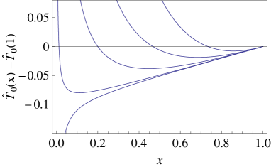
Figure 6: Dependence of temperature profiles $\hat{T}_{0}(x)-\hat{T}_{0}(1)$ on the rotation speed according to (71). A larger $\epsilon$ means a bigger deviation of $v_{2}$ from its reference values. From bottom to top: $\epsilon=0.78$ (no cooling is present, since neither (56), nor (57) hold), $\epsilon=0.81$, $\epsilon=1$, $\epsilon=1.5$ and $\epsilon=3$. The latter four curves demonstrate cooling. For other parameters we take [cf. Figs. 2 and 3]: $\hat{T}^{\prime}_{0}(1)=0.1$, $\alpha=1$, $b=-1$, $\kappa=-0.5$.

Fig. 6 shows temperature profiles (71) for different values of $\epsilon$ and for parameters given by (58, 62). For given values of parameters, there is a value of $v_{2}$, where the cooling effect is maximal, i.e. the lowest temperature is reached. For the parameters of Fig. 6 this critical value is found from $\epsilon=0.8$. When $v_{2}$ decreases from this critical value, the cooling effect ceases to exist, since the cooling boundary conditions—as given by (56) or (57)—cannot hold anymore, i.e. the curve in Fig. 6 that corresponds to $\epsilon=0.78$ is void of physical meaning. When $v_{2}$ increases from the critical value, the magnitude of vortex cooling—as measured by the lowest temperature reached—monotonously decreases. In particular, for a larger $\epsilon$, we need to take a larger $x_{0}=r_{1}/r_{2}$ (i.e. $x_{0}\to 1$) to achieve cooling; see Fig. 6.

V Relations with experiments

V.1 Effective viscosity

The actual flow in vortex tubes is highly turbulent gutsol . Hence if one uses hydrodynamic equations (in particular, Navier-Stockes equations) with constant values of viscosities $\eta$ and $\zeta$ and heat-conductivity $\lambda$, it is at very least necessary to employ there effective (i.e. turbulent or non-molecular) estimates for these parameters landau ; shirokov .

Taking into account that the considered flow is confined and inhomogeneous (i.e. there are radial and angular flows) we choose to estimate the turbulent viscosity $\eta$ via the Nusselt’s formula nusselt , which was originally proposed for estimating the turbulent viscosity in pipes. Ref. shirokov found that this formula applies for describing compressible turbulence in a sufficiently wide range of Reynolds numbers. The formula reads nusselt ; shirokov :

$$\eta=0.15\,\eta_{\rm mol}\left[\,\rho\,v_{\phi}\,l\,/\eta_{\rm mol}\,\right]^{3/4},$$ (72)

where $v_{\phi}$ is the characteristic value of the angular velocity, and $l$ is the characteristic length, and $\eta_{\rm mol}$ is the molecular viscosity: $\eta_{\rm mol}=1.8\times 10^{-5}$ kg/(m s) for the air. Also, taking in (72) typical experimental parameters for vortex tubes savino : $\rho=1.2$ kg/${\rm m}^{3}$, $v_{\phi}\simeq v_{\rm sound}=$331 m/s and $l=0.1$ m, we get

$$\eta\sim 0.085\,\,{\rm kg/(m\,s)},$$ (73)

which is several orders of magnitude larger than $\eta_{\rm mol}$. The estimate (73) roughly coincides with an estimate given in knoer via the mixing-length formula shirokov : $\eta=\rho\ell^{2}\frac{{\rm d}v_{\phi}}{{\rm d}r}$, where $\ell=\beta\frac{{\rm d}v_{\phi}}{{\rm d}r}\left/\frac{{\rm d}^{2}v_{\phi}}{{\rm d}r^{2}}\right.$ is the mixing length and where $\beta$ is a suitable numerical constant. It is this specific form of the mixing-length formula that can apply to compressible turbulence shirokov .

V.2 Comparison with experiment

Let us recall that the present model omits several physical factors that are met in realistic vortex tubes; see section I for a discussion of basic set-ups for vortex tubes. In particular, the axial motion is neglected, and the fluid is removed radially (in contrast to axial removal in vortex tubes). Hence the model set-up has one (not two) output temperatures, and the whole outgoing fluid is cooled (in contrast to the standard Ranque tube which has two output flows and achieves temperature separation gutsol ).

Taking into account (27), the magnitude of cooling is predicted from (63) to be around 10 K. Note that best vortex tubes provide (starting from 300 K) a larger cooling of order 70-80 K hilsch ; graham ; gutsol . Though such a stronger effect is lacking in the present model, we recall that in those cases only a part (e.g. $\sim 20$ % according to hilsch ) part of the overall flow is strongly cooled, the remaining part is heated up. In the present model the whole outgoing fluid is cooled.

The Hilsch efficiency $\xi_{\rm H}$ of cooling obtained in the present model is of order of $0.1-0.4$; see Figs. 2-4. It also agrees with experiments, though not for the most efficient vortex tubes, where $\xi_{\rm H}$ can be as high $0.6-0.7$ hilsch ; gutsol .

The magnitude of the radial flow over the angular flow, expressed by

$$w(1)=10^{-3}-10^{-4},$$ (74)

also agrees with experimental measurements gutsol ; xue , though it is to be stressed that these measurements were carried out for sufficiently long vortex tubes, where the axial velocities (neglected altogether in the present model) are definitely larger than the radial velocities. The quasi-solid vortex (58) for $\hat{v}_{\phi}(x)$ is also seen experimentally, though the experimental results also indicate that for $x\sim 1$, $\hat{v}_{\phi}(x)$ starts to decay, i.e. the quasi-solid vortex $\hat{v}_{\phi}(x)\sim x^{1+\kappa}$ (for our model we took $\kappa\sim-0.5$) changes towards the potential vortex $\hat{v}_{\phi}(x)\sim x^{-1}$ gutsol ; xue . This change of $\hat{v}_{\phi}(x)$ is given much importance in certain theories of vortex cooling graham ; gutsol , but is not present here.

The input density is estimated from (4, 21):

$$\rho(r_{2})=\frac{|\kappa|\,\eta}{w(1)\,r_{2}\,v_{\phi}(r_{2})}.$$ (75)

Estimating $r_{2}\simeq 0.1$ m (reasonable value for the outer radius of a vortex tube), $v_{\phi}(r_{2})\simeq v_{\rm sound}$ and $\eta$ for air as $\eta\simeq 0.085$ kg/(m  s) [see 73], we end up with $\rho(r_{2})\simeq\frac{10^{-3}}{w(1)}$ kg/(m  s) in (75). Estimating from the present model $w(1)\simeq 10^{-4}$ (and recalling $p=R\rho T/\mu$) we get that the input pressure is few times larger than the atmospheric pressure ranque .

Altogether, given limitations of the present model, and complications of the flow in real vortex tubes, one can say that the model is in a fair qualitative agreement with experiments, though it is far from predicting (and explaining) the features of best vortex tubes, those providing the largest efficiency or the largest magnitude of cooling.

Savino and Ragsdal presented a simplified set-up of vortex cooling effect savino that in several respects is similar to the present model. They studied two short (compared to the diameters) concentric cylinders; the length to diameter ratio was $0.1$ and $0.5$ for two different samples. (For traditional Ranque-Hilsch tubes the length to diameter ratio is 20–50). The rotating air enters radially from the whole outer permeable cylinder and leaves through the inner (smaller) cylinder. Rotational flow was created via the outer cylinder with Mach number $\simeq 0.2$. The velocity of this flow was much larger than that of the radial flow. The authors found a cooling effect in terms of the radial variation of the stagnation enthalpy (no data on thermodynamic temperature or velocities was given). The magnitude of this cooling effect is lower than predictions of the present model; cf. the stagnation enthalpy data in Figs. 2–3. They confirmed that the radial distribution of the stagnation enthalpy is established already near the end-wall of the tube and is not affected by the weak axial flow. In particular, the axial change of the stagnation enthalpy was much smaller than the radial one. (Hence it was legitimate to neglect the axial flow in the model.) They found that the experimental data can be described by (54), where pressure is balanced by the centrifugal force (this equation does not contain the viscosity explicitly). It was observed that the pressure decreases monotonically with the radius, as confirmed by (55) of the present model.

VI Cooling of outward flow

VI.1 Conditions for cooling

Now we assume that $c>0$ (i.e. $\kappa>0$ and $b>0$) and the outer boundary of the system is thermally isolated in the sense of (47). Hence the outgoing fluid being colder than in-coming one, this implies (for $c>0$) $\hat{T}^{\prime}(1)<0$, and then (47) demands

$$\hat{T}^{\prime\prime}(1)>0,$$ (76)

at the adiabatic outer boundary. No specific conditions are imposed at the inner boundary $r=r_{1}$ that can be thus considered as a control surface.

The full expression for $\hat{T}^{\prime\prime}(1)$ is worked out from (18, 19) [recall (25)]:

$$\hat{T}^{\prime\prime}(1)=\frac{b\hat{T}^{\prime}(1)w^{\prime}(1)}{\hat{c}_{p}w(1)}+[\frac{b(\hat{c}_{p}-1)}{\hat{c}_{p}}-1]\hat{T}^{\prime}(1)$$ (77)

$$-(\chi+\frac{1}{3})w^{\prime}(1)^{2}-(2w(1)-w^{\prime}(1))^{2}-(\alpha(2+\kappa)-2)^{2}.$$ (78)

The first line (77) contains potentially positive terms, while all terms in (78) are non-positive. Hence (76) demands that (78) is sufficiently small, e.g. via $w^{\prime}(1)\to 0$. Likewise, $\hat{T}^{\prime}(1)$ cannot be very small.

If $w(x)$ and $w^{\prime}(x)$ are sufficiently small, $\hat{T}(x)$ can be approximately determined from (53, 52). However, (54, 55) do not apply anymore, because the (dimensionless) pressure $\hat{p}(x)=\hat{T}(x)/w(x)$ is now a decreasing function of $x$ for $x\in[x_{0},1]$. Thus, $w(x)$ is now essential in (19) and it is important for determining the energetics. The physical reason for this is that the work $\Delta\widehat{W}_{r}$ [see (31)] done by viscous radial forces is relevant, as seen below.

Fig. 7 demonstrates the main outward-flow cooling scenario for $\alpha=1$; cf. (8). The magnitude of cooling is now sizable

$$[\hat{T}(x_{0})-\hat{T}(1)]/\hat{T}(x_{0})\geq 10.$$ (79)

The temperature profile $\hat{T}(x)$ shown in Fig. 7 coincides with that found from (59, 60), where now $\hat{T}^{\prime}(1)<0$ and $x_{\rm min}$ in (60) should be changed to $x_{\rm max}$, because this is now the maximum of $\hat{T}(x)$. Then one should take $x_{0}>x_{\rm max}$ so that the temperature decreases for $x_{0}<x<1$.

VI.2 Energetics, entropy and efficiency

We expectedly have

$$\widehat{Q}(x_{0})=-x_{0}\hat{T}^{\prime}(x_{0})>0,\qquad\widehat{Q}(1)=-\hat{T}^{\prime}(1)>0,$$ (80)

i.e. the heat enters from the inner boundary $x=x_{0}$ and leaves at the outer boundary $x=1$; see (48). We see numerically that $\hat{Q}_{1}\lesssim\hat{Q}_{2}$; see Fig. 7.

Now $\Delta\widehat{W}_{\phi}<0$ (rotating cylinders invest work), as we discussed after (30). But the radial external forces do extract work, $\Delta\widehat{W}_{r}>0$ as much that the total work is extracted [see Figs. 7, 8]:

$$\Delta\widehat{W}=\Delta\widehat{W}_{r}+\Delta\widehat{W}_{\phi}>0.$$ (81)

Moreover, the overall kinetic energy (see (29)) also increases, $\Delta\widehat{E}_{\rm kin}>0$ (albeit slightly, as seen in Fig. 7) due to contribution $\frac{\kappa}{2}(1-x_{0}^{2+2\kappa})$ of the vortex.

The most interesting aspect of this cooling scenario is that the cooling efficiency (37) is larger than $1$ [see Fig. 7]:

$$\xi\geq 1,$$ (82)

i.e. the adiabatic process provides less cooling, since now the heat transfer from the system is essential; see after (45). Together with (82), the Hilsch efficiency (38) is also larger than 1: $\xi_{\rm H}>1$; see Fig. 7.

Eq. (82) is thermodynamically consistent. Recalling (39, 43), we see that the upper bound (45) amounts to $\frac{x_{0}\hat{T}^{\prime}(x_{0})}{\hat{T}(x_{0})}-\frac{\hat{T}^{\prime}(1)}{\hat{T}(1)}$. This expression is positive; cf. (80). Hence it is possible to have (82) provided that the entropy production is sufficiently small, which appears to be the case, as confirmed numerically. We stress again that $\xi>1$ is possible due to heat conductivity; cf. the discussion after (45).

Due to (39) and (82), the entropy entering to the system is larger than the one that leaves it [cf. (65)]:

$$s(r_{2})-s(r_{1})=c_{p}\ln[1/\xi].$$ (83)

Thus we get that (without any investment of overall external work) the temperature, stagnation enthalpy and entropy decrease, while the kinetic energy increases. The outgoing fluid is more ordered, since not only its thermal energy decreases, but also the kinetic energy increases.

VI.3 Physical mechanisms of the effect and cooling without vortical motion

We saw around (68, 69) that in order to get inward flow cooling it is necessary to have an angular motion with the viscous forces doing work of the proper sign. Here the physical meaning of cooling can be clarified along the same lines. We get from (18) and (29–32)

$$0=\left[\widehat{E}(x)+\widehat{Q}(x)+\widehat{W}_{r}(x)+\widehat{W}_{\phi}(x)\right]^{\prime}.$$ (84)

Now cooling implies that outgoing fluid has lower energy: $\widehat{E}^{\prime}(x)<0$. Possible necessary conditions for cooling is provided by the heat conductivity: $\widehat{Q}^{\prime}(x)>0$, and/or by the work done via radial viscosity: $\widehat{W}_{r}^{\prime}(x)>0$. Figs. 7 and 8 show that both these conditions hold. The contribution of $\widehat{Q}^{\prime}(x)>0$ is larger than that of $\widehat{W}_{r}^{\prime}(x)>0$.

But the vortex contribution has the same sign as energy: $\widehat{W}_{\phi}^{\prime}(x)<0$; cf. with (69). Hence a similar cooling scenario is also possible without vortex, i.e. for $\hat{v}_{\phi}=0$ in (18, 19). In fact, eliminating the angular motion almost does not change the temperature profile in Fig. 7. The main difference with the above situation is that the kinetic energy decreases, $\Delta E_{\rm kin}<0$, since the vortex motion is now absent.

Note that to eliminate the vortex from equations of motion, one should take $v_{\phi}=0$ in (18, 19), and to suppress the last factor $-\alpha(2+\kappa)+2+\frac{\kappa}{2}$ in (25), as well as $-(\alpha(2+\kappa)-2)^{2}$ in (78). Definitions (21, 22, 23) of dimensionless parameters still apply, where now $v_{2}=v_{2,0}$ is an arbitrary characteristic velocity; see section IV.7. It drops out from (18, 19).

A simple analytical description of the temperature profile can be obtained from (18) assuming that the change of $w(x)$ can be neglected. (But note that the change of $w(x)$ within (19) cannot be neglected.) Taking in (18) $\hat{v}_{\phi}=0$, $w(x)=w(1)$ and $w^{\prime}(x)\to 0$, we get

$$\hat{T}(x)-\hat{T}(1)=\gamma[1-\frac{1}{x^{2}}]+[2\gamma-\hat{T}^{\prime}(1)]\,\frac{1-x^{b}}{b},$$ (85)

$$\gamma\equiv\frac{w(1)^{2}(4+\kappa)}{2(2+b)}.$$ (86)

Now $\hat{T}^{\prime}(x)=0$ is solved as $x_{\rm max}^{b+2}=\frac{2\gamma}{2\gamma-\hat{T}^{\prime}(1)}$. This solution exists only for $\hat{T}^{\prime}(1)<0$ (recall that $b>0$) and it is a maximum of $\hat{T}(x)$. Hence one should take $x_{0}>x_{\rm max}$ in order to get a monotonic decrease of temperature $\hat{T}(x)$ from $x=x_{0}$ till $x=1$.

One feature of this cooling scenario is that once $w(1)$ (the boundary condition for the outward flow) decreases, the solution of hydrodynamic equations (18, 19)) ceases to exist below a certain critical value of $w(1)$, because now $w(x_{0})$ becomes negative. Recall from (4) that a negative $w(x_{0})$ for $c>0$ is not acceptable, since it would mean a negative mass density $\rho$. Thus, if $w(1)$ is decreased, then $c$ also has to decrease, to keep the solution physical.

Generally, the magnitude (79) of the cooling increases upon decreasing the radial flow $c$, i.e. for $c\to 0$. This can be seen from (85) or from Figs. 8. But this limit $c\to 0$ is not useful, since it diminishes the cooling power $b(\hat{T}(x_{0})-\hat{T}(1))$.

VI.4 Geometric aspects of the cooling effect

Note that the present cooling scenario (without vortex) is specific for the cylindrical geometry. Its traces are seen in 1d (plane geometry), but the cooling as such is negligibly weak there; see Appendix C.

To understand the origin of this effect, let us take the situation, where all the velocities vanish (hence $c=0$). Due to the cylindrical geometry, (12) shows that there is still a non-trivial stationary temperatures profile, $c_{\rm e}=-\lambda rT_{0}^{\prime}$ that reads in terms of the dimensionless temperature $\hat{T}$ and dimensionless length $x=r/r_{2}$ ($x_{0}\leq x\leq 1$):

$$\hat{T}_{0}(x)-\hat{T}_{0}(1)=\hat{T}^{\prime}_{0}(1)\ln x.$$ (87)

Now it should be clear that (87) does not describe as such any cooling effect. Indeed, for $\hat{T}^{\prime}_{0}(1)\leq 0$ we should put a thermally isolated wall at $x=1$ (to avoid assuming the existence of even colder temperatures), which leads us to $\hat{T}^{\prime}_{0}(1)=0$, and hence to a constant temperature profile.

However, there is a relation between (87) and the temperature profiles obtained above for $c>0$ and illustrated in Figs. 7, and 8:

$$\hat{T}_{0}(x)>\hat{T}(x),$$ (88)

$${\rm if}~{}~{}~{}\hat{T}^{\prime}_{0}(1)=\hat{T}^{\prime}(1)<0~{}~{}~{}{\rm and}~{}~{}~{}\hat{T}_{0}(1)=\hat{T}(1),$$ (89)

where we note from (87) that $\hat{T}^{\prime\prime}_{0}(1)=-\hat{T}^{\prime}_{0}(1)$, i.e. for $\hat{T}^{\prime}_{0}(1)=\hat{T}^{\prime}(1)<0$, $\hat{T}_{0}^{\prime\prime}(1)$ agrees with the boundary condition (47) required for cooling.

Eqs. (88, 89)—which we verified numerically—show that the reported cooling effect is the modification of the formal temperature profile (87) to the physical, situation with $c>0$. In the 1d case (plane geometry) the general zero-velocity temperature profile (the analogue of (87)) is just $T_{0}={\rm const}$, which explains why the cooling effect is negligible there; see Appendix C.

VII Summary

We worked out a tractable model for describing gasodynamic cooling. The model extends the standard Couette flow between two coaxial cylinders by adding there a radial flow (hence demanding that cylinders are permeable). Only the radial dependence of relevant quantities is retained and the axial flow is neglected.

The model accounts for viscosity, heat-conductivity and compressibility; see section II. They are generally important for gasodynamic cooling, and there are at least two reasons for keeping each of them in the description. Viscosity is to be retained, (first) since we should achieve cooling also in terms of the stagnation enthalpy (as observed experimentally savino ), and (second) since due to turbulence the actual viscosity is much larger than its molecular value. Heat-conductivity is to be considered simultaneously with viscosity, since the Prandtl number of air is close to one. It is also important for ensuring boundary conditions of cooling. Compressibility is needed, because we need the proper relation between fluid mechanics and thermodynamics, and also because the involved angular velocities are sonic.

The emphasize of our study is not so much in describing details of the vortex cooling effect as observed in experimental examples of vortex tubes, but rather in showing how a hydrodynamic model can account for cooling via specific boundary conditions (see section III), and how already the simplest model can provide new (and thermodynamically consistent) predictions for cooling with efficiency larger than $1$.

We show that the model predicts a vortex cooling effect for an inward radial flow; see section IV. Though the general cause of cooling is in the pressure gradient that drives the flow, the local cause is related to the work done by viscous forces. The cooling effect comes in two versions—adiabatic and isothermal—that are closely related, but differ from each other by the boundary conditions. In several ways the obtained cooling effect is similar to what was experimentally seen in Ref. savino for a short uniflow vortex tube. In accordance with experimental results, the model predicts that the efficiency of vortex cooling is generically smaller than 1 [see section II.7], though the concrete values for the efficiency and for the magnitude of cooling are lower than what was observed for best vortex tubes.

The model predicts as well a cooling effect that was (to our knowledge) so far not observed experimentally; see section VI. This effect is realized for an outward flow and it does not need an angular (vortical) motion. Its cooling efficiency is larger than one, i.e. for the given gradient of pressure, this cooling is more efficient than the adiabatic (i.e. entropy conserving) thermodynamic process. This cooling effect is consistent with the second law, and it is possible due to heat-conductivity. It has partly a geometric origin, since it is negligible for the plane geometry.

There is an experimental report on the Hilsch efficiency being larger than 1 for a counter-flow tube (where only a part of the air is cooled) martyn . However, this result was was not reproducible in guliguli . According to the author of Ref. guliguli , the report concerned externally cooled vortex tubes; cf. our discussion in section III. Hence we conclude by stressing that cooling with an efficiency larger than one is an open problem.

Appendix A Ideal gas thermodynamics

We briefly recall ideal-gas formulas as applied in hydrodynamics. Thermodynamic relations of hydrodynamics are written for extensive quantities are divided by the overall number $N$ of involved particles and by the mass $m$ of a single particle. Thus the extensive ideal gas entropy

$$S=k_{\rm B}C_{v}\ln[p]+k_{\rm B}C_{p}\ln[V/(Nm)],$$ (90)

where $C_{v}$ and $C_{p}$ are heat-capacities and $V$ is the volume, becomes

$$s=\frac{S}{Nm}=\frac{k_{\rm B}}{m}\frac{C_{v}}{N}\ln[p]+\frac{k_{\rm B}}{m}\frac{C_{p}}{N}\ln[V/(Nm)]$$

$$=\frac{k_{\rm B}N_{A}}{N_{A}m}\hat{c}_{v}\ln[p]-\frac{k_{\rm B}N_{A}}{N_{A}m}\hat{c}_{p}\ln[\rho],$$ (91)

where $\rho=Nm/V$ is the mass density, $N_{A}$ is the Avogadro number, and where $\hat{c}_{v}$ and $\hat{c}_{p}$ are dimensionless numbers of order one:

$$\hat{c}_{p}-\hat{c}_{v}=1.$$ (92)

After denoting

$$k_{\rm B}N_{A}=R,\qquad N_{A}m=\mu,$$ (93)

where $R=8.314$ J/K is the gas constant, and $\mu$ is the molar mass, (91) reads:

$$s={c}_{v}\ln[p]-{c}_{p}\ln[\rho],$$ (94)

$$c_{v}=(R/\mu)\,\hat{c}_{v},~{}~{}c_{p}=(R/\mu)\,\hat{c}_{p}.$$ (95)

The full entropy $S$ (and similarly other extensive quantities) is obtained as $S=\int_{V}{\rm d}^{3}x\,\rho\,s$. Noting that the temperature $T$ is measured in Kelvins, the ideal gas equation of state $pV=k_{\rm B}NT$ becomes

$$p=(R/\mu)\,\rho T.$$ (96)

For purposes of dimensionless analysis, we write (94) as

$$s=c_{p}\left(-\frac{1}{\hat{c}_{p}}\ln[p]+\ln[T]-\ln\left[\frac{\mu}{R}\right]\right).$$ (97)

Eq. (97) implies that if the pressure and temperature adiabatically (i.e. for a constant entropy) change as $p\to p^{\prime}$ and $T\to T^{\prime}$, then

$${T^{\prime}}/{T}=\left({p^{\prime}}/{p}\right)^{1/\hat{c}_{p}}.$$ (98)

Appendix B Vortex flow without radial motion (Couette flow)

Consider the distribution of temperature inside of the vortex (7) when the radial motion is absent. This is one of standard problems of hydrodynamics (the Couette flow) and it is studied in many places; see e.g. landau ; dorfman . We reconsider this problem here, because we want to understand why specifically this situation does not contain any interesting stationary cooling scenario (contrary to remarks given in dorfman ). For

$$v_{r}=c=w=\kappa=b=0,$$ (99)

we get $(\frac{\kappa}{2}+1)\hat{v}_{\phi}^{2}-x\hat{v}_{\phi}\hat{v}^{\prime}_{\phi}+b\hat{T}-x\hat{T}^{\prime}-\beta=0$ from (18). This equation integrates and determines temperature inside of the vortex ($x\equiv r/r_{2}$)

$$\hat{T}(x)=\hat{T}(1)-(1-\alpha)^{2}(\frac{1}{x^{2}}-1)$$

$$+(\hat{T}^{\prime}(1)-2(1-\alpha)^{2})\ln x,~{}~{}~{}~{}x_{0}\equiv\frac{r_{1}}{r_{2}}\leq x\leq 1,~{}~{}$$ (100)

where we employed (25, 99) for expressing $\beta$ via $\hat{T}^{\prime}(1)$, and where $\alpha$ is given by (9) under $\kappa=0$:

$$\alpha=\frac{1-(v_{1}r_{1})/(v_{2}r_{2})}{1-(r_{1}/r_{2})^{2}}.$$ (101)

Note that taking the inner radius $r_{1}$ to zero, $r_{1}\to 0$, does not lead to anything interesting: in this limit we get $\alpha\to 1$, (100) implies $\hat{T}(x)=\hat{T}(1)+\hat{T}^{\prime}(1)\ln x$, but we have to assume also $\hat{T}^{\prime}(1)=0$ for preventing the singularity at $x\to 0$. Then $\hat{T}(x)$ does not depend on $x$. Hence $r_{1}$ should be kept finite.

Interesting (stationary) cooling scenarios are those, where the low temperatures created inside of the fluid are not due to even lower temperatures imposed on its boundary. In particular, if one of the boundaries is left without thermal isolation—so there is an active thermal bath working at this boundary—then the inside temperature should be lower than the temperature of this bath.

Let us start with the case, where no thermal isolation is imposed for both boundaries. Then $\hat{T}(x)$ should have a local minimum at some $x\in(x_{0},1)$. Eq. (100) shows that there is only one solution $x=x_{\rm max}$ of $\hat{T}^{\prime}(x)=0$:

$$x_{\rm max}=\sqrt{\frac{2(1-\alpha)^{2}}{2(1-\alpha)^{2}-\hat{T}^{\prime}(1)}}.$$ (102)

If $0<x_{\rm max}<1$ (for which it is necessary and sufficient that $\hat{T}^{\prime}(1)<0$), then $x_{\rm max}$ is the local maximum (not minimum) of $\hat{T}(x)$. Hence we get no cooling for this case.

Next, let us thermally isolate the outer boundary: $\hat{T}^{\prime}(1)=0$. We get from (100):

$$\hat{T}(x)-\hat{T}(1)=-(1-\alpha)^{2}\left(\frac{1}{x^{2}}-1-\ln[\frac{1}{x^{2}}]\right).$$ (103)

Then $\hat{T}(x)$ is a monotonically increasing function of $x$, i.e. the inside temperature $\hat{T}(x)$ is larger than the (inner) bath temperature $\hat{T}(x_{0})$. For a thermally isolated inner boundary, $\hat{T}^{\prime}(x_{0})=0$, $\hat{T}(x)$ is a monotonically decreasing function of $x$ [see (102)], i.e. again we get no interesting scenarios of cooling. There are no solutions when both boundaries are thermally isolated; see (100).

The absence of interesting cooling scenarios is confirmed by looking at the total work produced by external forces that rotate the cylinders. It reads from (35) [with $\kappa=0$]:

$$\widehat{W}_{\phi}=2(1-\alpha)^{2}(1-\frac{1}{x_{0}^{2}})<0.$$ (104)

The negativity of (104) means that the work is invested externally and dissipated for overcoming the viscous forces. This work leaves the system as heat.

Thus three regimes are impossible for the considered Couette flow:

– It cannot cool the fluid isothermally, i.e. when both boundaries are kept at the same temperature.

– It cannot cool the fluid adiabatically: no regime exists when one boundary is thermally isolated, while another one is subject to a thermal bath, and it is demanded to get the fluid colder than the active bath temperature. Hence low-temperatures present in the system according to (100) do not constitute any non-trivial cooling: they are due to the low-temperature bath present at one of boundaries. Put differently, for the Couette flow the active bath is the one with the lower temperature.

The above two conclusions seem to hold rather generally for stationary hydrodynamic systems without mass flow, though we so far did not get a general argument for their validity. At any rate they hold for the (generalized) Couette (sometimes also called Taylor-Dean) flow, where the fluid is subject to azimuthal driving with a volume force $\vec{f}$, where only the $\phi$-component $f_{\phi}(r)$ of $\vec{f}$ is non-zero, but it is an arbitrary function of $r$.

– The Couette flow cannot also function as a heat-engine, since—irrespectively of the values of $T(r_{2})$ and $T(r_{1})$—the work is always dissipated; see (104).

Appendix C 1d example of weak adiabatic cooling

Consider a 1d flow (from left to right) between two permeable plates separated by distance $L$. Continuity of mass leads to

$$\rho v=c_{1}={\rm const}.$$ (105)

1d Navier-Stokes and energy equations read in dimensionless form

$$\kappa\hat{v}^{2}(x)+\frac{b}{\hat{c}_{p}}\hat{T}(x)-(\chi+\frac{4}{3})\hat{v}(x)\hat{v}^{\prime}(x)=\gamma\hat{v}(x),$$ (106)

$$\frac{\kappa}{2}\hat{v}^{2}(x)+b\hat{T}(x)-(\chi+\frac{4}{3})\hat{v}(x)\hat{v}^{\prime}(x)-\hat{T}^{\prime}=\beta,$$ (107)

where $0\leq x\leq 1$, $L$ is the distance between two plates, $\beta$ and $\gamma$ are constants, and we introduced the following dimensionless parameters:

$$\hat{T}=\frac{\lambda}{v_{2}^{2}\eta}T,~{}~{}\hat{v}(x)=\frac{v(x)}{v(L)}$$ (108)

$$b=\frac{c_{1}c_{p}L}{\lambda},~{}~{}~{}~{}\kappa=\frac{c_{1}L}{\eta},$$ (109)

$$\chi=\frac{\zeta}{\eta},~{}~{}~{}\hat{c}_{p}=c_{p}(\mu/R).$$ (110)

The constants $\beta$ and $\gamma$ can be expressed via (respectively) $\hat{v}^{\prime}(1)$ and $\hat{T}^{\prime}(1)$:

$$\gamma=\kappa+\frac{b}{\hat{c}_{p}}\hat{T}(1)-(\chi+\frac{4}{3})\hat{v}^{\prime}(1),$$ (111)

$$\beta=\frac{1}{2}\kappa+b\hat{T}(1)-(\chi+\frac{4}{3})\hat{v}^{\prime}(1)-\hat{T}^{\prime}(1).$$ (112)

We obtain from (108–111):

$$\hat{T}^{\prime\prime}(1)=b\hat{T}^{\prime}(1)(1-\frac{1}{\hat{c}_{p}})-(\chi+\frac{4}{3})\hat{v}^{\prime}(1)^{2}+\frac{b}{\hat{c}_{p}}\hat{T}(1)\hat{v}^{\prime}(1).$$ (113)

Let us now look at conditions for adiabatic cooling. Now $c_{1}>0$ (hence $b>0$ and $\kappa>0$) and $\hat{v}>0$ from (105). Hence we look for

$$\hat{T}(0)>\hat{T}(1),\qquad\hat{T}^{\prime\prime}(1)>0.$$ (114)

The temperature profiles appear to be monotonic so that the first condition in (114) can be written as $\hat{T}^{\prime}(1)<0$. Then the first and second term in the right-hand-side of (113) are negative. Hence $\hat{T}^{\prime\prime}(1)>0$ can be satisfied only due to sufficiently large $\frac{b}{\hat{c}_{p}}\hat{T}(1)\hat{v}^{\prime}(1)>0$. This implies limitations on $T(1)$ (which cannot be sufficiently small) and on $|\hat{T}^{\prime}(1)|$ (which cannot be sufficiently large). Eventually, the adiabatic cooling appears to be a relatively small effect, though it is still possible in this model. For example, under $\chi=10$, $b=\kappa=10$, $\hat{c}_{p}=3.5$, $\hat{T}(1)=1$, $\hat{T}^{\prime}(1)=-0.1$ and $\hat{v}^{\prime}(1)=0.1$ (we have $\hat{v}(1)=1$ by definition) we get for the cooling magnitude $[\hat{T}(0)-\hat{T}(1)]/\hat{T}(0)=0.037$.

Appendix D Potential vortex

Another familiar type of vortex in (7, 8) is:

$$\alpha=0~{}~{}{\rm or}~{}~{}\frac{v_{1}}{v_{2}}=\frac{r_{2}}{r_{1}}.$$ (115)

Eqs. (53, 52) imply

$$\hat{T}(x)-\hat{T}(1) = [\hat{T}^{\prime}(1)-\frac{\kappa+4}{b+2}]\,\,\frac{x^{b}-1}{b}$$ (116)

$$+ \frac{\kappa+4}{2(b+2)}(1-x^{-2}).$$

Now $\hat{T}^{\prime}(x)=0$ is solved as

$$x^{-2-b}=1-\frac{(b+2)T^{\prime}(1)}{(w^{2}(1)+1)(\kappa+4)}.$$ (117)

Hence the minimum of $\hat{T}(x)$ for $\hat{T}^{\prime}(1)>0$ can exist only for

$$\kappa<-4,$$ (118)

i.e. only for radially inward flowing fluid ($c<0$).

Now the isothermal cooling is driven by the work done for rotating cylinders. Eqs. (35, 115) imply

$$\widehat{W}_{\phi}=2(1-x_{0}^{-2})<0,$$ (119)

while the kinetic energy change is now larger than zero; see (67, 115). Due to this, $\hat{U}(x_{0})>\hat{U}(1)$.

In other respects the two scenarios of cooling (quasi-solid and potential) are similar to each other: both have roughly the same magnitude, both need small radial velocities and both have efficiency $\xi$ smaller than $1$.

Figures

Figure 1: Cross-section of the flow: two coaxial permeable cylinders with radii $r_{1}$ and $r_{2}$ rotate with prescribed speeds. Solid vectors $\vec{v}_{\phi}={v}_{\phi}\vec{e}_{\phi}$ and $\vec{v}_{r}={v}_{r}\vec{e}_{r}$ refer to the velocity components of the flow for $r_{1}<r<r_{2}$. Here the radial flow is directed from the outer (larger) cylinder to the inner (smaller) cylinder. Now $|\vec{v}_{r}|<|\vec{v}_{\phi}|$, since the radial flow has to be smaller for cooling.

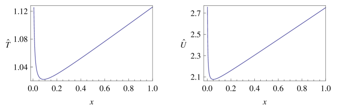
Figure 2: Isothermal cooling with inward flow ($c<0$) and quasi-solid vortex; see section IV.3. Dimensionless temperature $\hat{T}(x)$ and dimensionless stagnation enthalpy $\hat{U}(x)$ versus dimensionless distance $x$.
Left (right) figure: $\hat{T}(x)$ ($\hat{U}(x)$) versus $x=r/r_{2}$ for $x\in[x_{0},1]$, where $x_{0}=0.007347$.
The curves are obtained from numerical solution of (18, 19) for $\alpha=1$, $\kappa=-0.5$, $b=-1$, $\hat{c}_{p}=3.5$, $\beta=-1$ ($\hat{T}^{\prime}(1)=0.124$), $\chi=10$ and $\hat{T}(1)=1.126$, $w(1)=10^{-4}$, $w^{\prime}(1)=0$. These parameter values are consistent with experiments savino ; see (27), (62) and the related discussion, as well as (72), (74) and the related discussion.
The minimal dimensionless temperature is $\hat{T}_{\rm min}=\hat{T}(x_{\rm min})=1.0223$, $x_{\rm min}=0.008891$.
The energy values are: $\Delta\widehat{E}=-0.24699$, $\Delta\widehat{W}=0.48228$, $\Delta\widehat{W}_{r}=-0.01405$, $\widehat{Q}(x_{0})=-x_{0}\hat{T}^{\prime}(x_{0})=0.11129$, $\widehat{Q}(1)=-\hat{T}(1)=-0.124$; cf. (29–33).
The pressure $p(x)$ is a monotonically increasing function of $x\in[x_{0},1]$; cf. (55). $\hat{T}_{\rm ad}(x_{\rm min})=0.73556$. The Hilsch efficiency is $\xi_{\rm H}=0.26559$; cf. (38).
Upon decreasing the initial temperature, $x_{\rm min}$ increases, while both the magnitude and quality of cooling decrease, e.g. for $\hat{T}(1)=1.16$ we get $x_{\rm min}=0.50597$, $\hat{T}_{\rm min}=\hat{T}(x_{\rm min})=1.13083$ and $\xi_{\rm H}=0.13016$.
$w(x)$ (and hence $w(x)/x$) is a monotonically decreasing function of $x\in[x_{0},1]$. Thus condition (50) holds for the inner wall. Condition (49) for the outer wall cannot hold simultaneously with (50); this is why a permeable wall is not imposed at $r=r_{2}$. The latter is just a control surface within which we describe the flow.

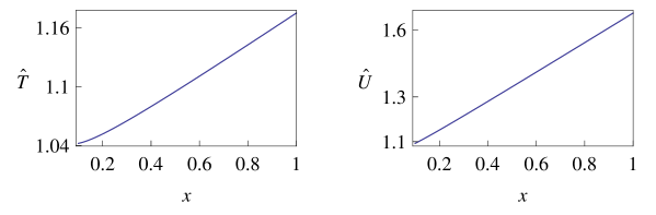
Figure 3: Adiabatic cooling with inward flow ($c<0$) and quasi-solid vortex. Dimensionless temperature $\hat{T}(x)$ and dimensionless stagnation enthalpy $\hat{U}(x)$ versus dimensionless distance $x$.
Left (right) figure: $\hat{T}(x)$ ($\hat{U}(x)$) versus $x=r/r_{2}$ for $x\in[x_{0},1]$, where $x_{0}=0.1$.
The curves are obtained from numerical solution of (18, 19) for $\alpha=1$, $\kappa=-0.5$, $b=-0.5$, $\hat{c}_{p}=3.5$, $\beta=-0.5$, $\chi=10$ and $\hat{T}(1)=1.175$, $w(1)=10^{-4}$, $w^{\prime}(1)=0$.
The minimal temperature is $\hat{T}(x_{0})=1.04233$. As required for an adiabatic, permeable inner boundary: $\hat{T}^{\prime\prime}(x_{0})=1.48034$; cf. (47, 48).
The energy values are: $\Delta\widehat{E}=-0.291278$, $\Delta\widehat{W}=0.44866$, $\widehat{Q}(x_{0})=-x_{0}\hat{T}^{\prime}(x_{0})=-0.0051$, $\widehat{Q}(1)=-\hat{T}^{\prime}(1)=-0.1625$; cf. (29–33).
Efficiency: $\hat{T}_{\rm ad}(x_{0})=0.52012$; see (36, 42). The Hilsch efficiency is $\xi_{\rm H}=0.2026$. Pressure $p(x)$ and $w(x)$ hold $p^{\prime}(x)>0$ and $w^{\prime}(x)<0$ for $x\in[x_{0},1]$.

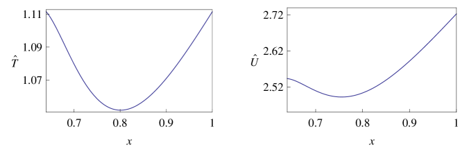
Figure 4: Isothermal cooling with inward flow and $\alpha=-0.5$ vortex. Dimensionless temperature $\hat{T}(x)$ and dimensionless stagnation enthalpy $\hat{U}(x)$ versus dimensionless distance $x$.
Left (right) figure: $\hat{T}(x)$ ($\hat{U}(x)$) versus $x=r/r_{2}$ for $x\in[x_{0},1]$, where $x_{0}=0.639472$.
The curves are obtained from numerical solution of (18, 19) for $\alpha=-0.5$, $\kappa=-4$, $b=-5$, $\hat{c}_{p}=3.5$, $\beta=-7$, $\chi=10$ and $\hat{T}(1)=1.1115$, $w(1)=0.01$, $w^{\prime}(1)=0$.
The minimal dimensionless temperature is $\hat{T}_{\rm min}=1.05166$ and it is reached for $x_{\rm min}=0.80077$.
The energy values are: $\Delta E=-1.62148$, $\Delta W=2.26812$, $\Delta W_{r}=-0.01403$, $\widehat{Q}(x_{0})=-x_{0}\hat{T}^{\prime}(x_{0})=0.204143$, $\widehat{Q}(1)=-\hat{T}^{\prime}(1)=-0.4425$.
The pressure $\hat{p}(x)$ ($w(x)$) is a monotonically increasing (decreasing) functions of $x\in[x_{0},1]$. $\hat{T}_{\rm ad}(x_{0})=0.952581$; see (36, 42). The Hilsch efficiency is $\xi_{\rm H}=0.376542$; cf. (38).

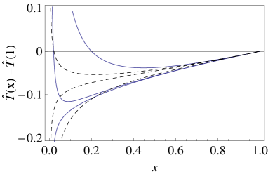
Figure 5: Dependence of the dimensionless temperature $\hat{T}(x)$ profiles [see (53)] on the radial Reynolds number, where the Prandtl number ${\rm Pr}=b/\kappa=2$ is fixed, the quasi-solid vortex condition $\alpha=1$ is obeyed [see (58)], and $\hat{T}^{\prime}(1)=0.1$.
Full, blue curves from top to bottom: $\kappa=-0.5$, $\kappa=-0.72$ and $\kappa=-0.725$. The first curve holds condition (56) for all $x_{0}$, the second one holds them for $x_{0}<0.21$, while the latter curve (with $\kappa=-0.725$) is void of physical meaning, since neither the adiabatic boundary condition (56), nor the isothermal condition (57) are satisfied for it.
Dashed, black curves from top to bottom: $\kappa=-0.3$, $\kappa=-0.25$ and $\kappa=-0.15$. For the curve with $\kappa=-0.25$ the adibatic boundary condition (56) holds for $x_{0}>0.447$. The whole curve with $\kappa=-0.15$ is void of the physical meaning, since neither (56), nor (57) hold.

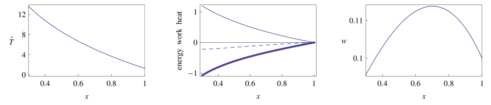
Figure 7: Adiabatic cooling with weak outward radial flow and quasi-solid vortex. Dimensionless temperature $\hat{T}(x)$, energy quantities and dimensionless radial velocity $w$ versus dimensionless distance $x$; see Table 1.
Eqs. (18, 19) are solved numerically for $\alpha=1$, $\kappa=0.1$, $b=0.1$, $\hat{c}_{p}=3.5$, $\beta=11$ ($\hat{T}^{\prime}(1)=-10.7867$), $\chi=10$, $\hat{T}(1)=1.295$, $w(1)=0.1$, and $w^{\prime}(1)=-0.1$ in the range $x=r/r_{2}\in[x_{0},1]$, where $x_{0}=0.3$.
Left figure: $\hat{T}(x)$ versus $x=r/r_{2}$ (the dimensionless stagnation enthalpy $\hat{U}(x)$ behaves similarly). A nearly identical temperature profile is obtained upon solving (18) with $w(x)=w(1)$ and $w^{\prime}(x)=0$.
Middle figure: the dimensionless energy $\widehat{E}(x)-\widehat{E}(1)$ (solid line), radial work $\widehat{W}_{r}(x)-\widehat{W}_{r}(1)$ (dashed line) and heat $\widehat{Q}(x)-\widehat{Q}(1)$ (bold line) versus $x$.
Right figure: $w(x)$ versus $x$. Condition (49) holds. It is written as $w(x_{0})>x_{0}w^{\prime}(x_{0})$ and $w(1)>w^{\prime}(1)$. The radial velocity $\propto w(x)/x$ is a monotonically decreasing function of $x$.
The minimal (maximal) dimensionless temperature is $\hat{T}(1)=1.295$ ($\hat{T}(x_{0})=13.6389$) and $\hat{T}^{\prime\prime}(1)=9.98$.
Energetics: $\Delta\widehat{E}=-1.1925$, $\Delta\widehat{E}_{\rm kin}=0.04188$, $\Delta\widehat{W}_{r}=0.21743$, $\Delta\widehat{W}=0.1245$, $\widehat{Q}(x_{0})=-x_{0}\hat{T}^{\prime}(x_{0})=9.7187$, $\widehat{Q}(1)=-\hat{T}^{\prime}(1)=10.885$.
Efficiency: $\hat{T}_{\rm ad}(1)=6.8718>\hat{T}(1)=1.295$ and the Hilsch efficiency is $\xi_{\rm H}=1.8241$. The pressure $p(x)$ is a decreasing function of $x$.

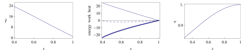
Figure 8: Adiabatic cooling with outward ($c>0$) radial flow and without vortex motion ($v_{\phi}=0$). Dimensionless temperature $\hat{T}(x)$, energy quantities and dimensionless radial velocity $w$ versus dimensionless distance $x$; see Table 1.
The curves are obtained from numerical solution of (18, 19) for $\kappa=1$, $b=1$, $\hat{c}_{p}=3.5$, $\beta=40$ ($\hat{T}^{\prime}(1)=-36.5$), $\chi=10$ and $\hat{T}(1)=1$, $w(1)=1$, $w^{\prime}(1)=0$.
Left figure: $\hat{T}(x)$ versus $x=r/r_{2}$ for $x\in[x_{0},1]$, where $x_{0}=0.4$ (the dimensionless stagnation enthalpy $\hat{U}(x)$ behaves similarly).
Middle figure: dimensionless energy $\widehat{E}(x)-\widehat{E}(1)$ (solid line), radial work $\widehat{W}_{r}(x)-\widehat{W}_{r}(1)$ (dashed line) and heat $\widehat{Q}(x)-\widehat{Q}(1)$ (bold line) versus $x$.
Right figure: $w(x)$ versus $x$. Condition (49) holds; cf. the data for Fig. 7. It also holds that $[w(x)/x]^{\prime}<0$.
The minimal dimensionless temperature is $\hat{T}(1)=1$ and $\hat{T}^{\prime\prime}(1)=6.4293$.
Energetics: $\Delta\widehat{E}_{\rm kin}=-1.8809$, $\Delta\widehat{W}=\widehat{W}_{r}=0.6676$, $\widehat{Q}(x_{0})=-x_{0}\hat{T}^{\prime}(x_{0})=12.9593$, $\widehat{Q}(1)=-\hat{T}^{\prime}(1)=36.5$.
Efficiency: $\hat{T}_{\rm ad}(1)=9.12373>\hat{T}(1)=1$ and the Hilsch efficiency is $\xi_{\rm H}=1.5719$. The pressure $p(x)$ is a decreasing function of $x$.

References

- (1) G. J. Ranque, Experiments on expansion in a vortex with simultaneous exhaust of hot air and cold air, J. Physique Radium, 4, 112 (1933).
- (2) R. Hilsch, The use of the expansion of gases in a centrifugal field as cooling process, Rev. Sci. Inst. 18, 108 (1947).
- (3) P.A. Graham, A theoretical study of fluid dynamic energy separation, Rep. No. TR-ES-721, George Washington Univ., Washington, DC, USA (1972).
- (4) A. Gutsol, The Ranque effect, Phys. Usp. 40, 639 (1997).
- (5) Y. Xue, M. Arjomandi and R. Kelso, A critical review of temperature separation in a vortex tube, Experimental Thermal and Fluid Science, 34, 1367 (2010).
- (6) A.I. Gulyaev, Vortex tubes and the vortex effect (Ranque effect), Soviet Physics Technical Physics 10, 1441 (1966).
- (7) R.T. Balmer, Pressure-Driven Ranque-Hilsch Temperature Separation in Liquids, Journal of Fluids Engineering, 110, 161 (1988).
- (8) V.E. Finko, Cooling and condensation of gas in a vortex flow, Soviet Physics Technical Physics, 28, 1089-1093 (1983). [Zhurnal Tekhnicheskoi Fiziki, 53, 1770-1776 (1983).]
- (9) T. Farouk, B. Farouk and A. Gutsol, Simulation of gas species and temperature separation in the counter-flow Ranque-Hilsch vortex tube using the large eddy simulation technique, Int. J. Heat and Mass Transfer 52, 3320 (2009).
- (10) J. P. Hartnett and E.R.G. Eckert, Experimental study of the velocity and temperature distribution in a high velocity vortex-type flow, Transactions of the ASME, 247-254 (Paper 55-A-108) (1957).
- (11) U. Behera, P.J. Paul, K. Dinesh and S. Jacob, Numerical investigations on flow behaviour and energy separation in Ranque-Hilsch vortex tube, Int. J. Heat and Mass Transfer 51, 6077 (2008).
- (12) A. Secchiaroli, R. Ricci, S. Montelpare, V. D’Alessandro, Numerical simulation of turbulent flow in a Ranque-Hilsch vortex tube, Int. J. Heat and Mass Transfer 52, 5496 (2009).
- (13) M.G. Dubinskii, Izvest. Akad. Nauk SSSR, Gas Flow in Rectilinear Channels, Otdel. Tekh. Nauk. 6, 47 (1955).
- (14) S. Eiamsa-ard and P. Promvonge, Review of Ranque-Hilsch effects in vortex tubes, Renewable and sustainable energy reviews, 12, 1822 (2008).
- (15) N.S. Torocheshnikov, I.L. Leites and V.M. Brodyanskii, A Study of the Effect of Temperature Separation of Air in a Direct-Flow Vortex Tube, Soviet Physics Technical Physics, 3, 1144 (1958). [Zhurnal Tekhnicheskoi Fiziki, 28, 1229 (1958).]
- (16) R. Liew, J. C. H. Zeegers, J. G. M. Kuerten, and W. R. Michalek, Maxwell’s Demon in the Ranque-Hilsch Vortex Tube, Phys. Rev. Lett. 109, 054503 (2012).
- (17) J. G. Polihronov and A. G. Straatman, Thermodynamics of Angular Propulsion in Fluids, Phys. Rev. Lett. 109, 054504 (2012).
- (18) T.S. Alekseev, The Nature of the Ranque Effect, Journal of Engineering Physics, 7, 121 (1964).
- (19) J.S. Hashem, A Comparative Study of Steady and Nonsteady-flow Energy Separators, Rep. No. RPI-TR-AE-6504, Rensselaer Polytechnic Inst., Troy NY, USA (1965).
- (20) M.V. Kalashnik and K. N. Visheratin, Cyclostrophic adjustment in swirling gas flows and the Ranque-Hilsch vortex tube effect, J. Exp. Theor. Phys. 106, 819 (2008).
- (21) A. P. Merkulov, A note on Alekseev’s article “The nature of the Ranque effect”, Journal of Engineering Physics and Thermophysics, 8, 474 (1965).
- (22) R. Kassner and E. Knoernschild, Friction laws and energy transfer in circular flow. Wright Patterson Air Force Base, Report PB-110936, parts I and II (1948). Available as http://www.dtic.mil/dtic/tr/fulltext/u2/a800229.pdf
- (23) J. J. van Deemter, On the theory of the Ranque-Hilsch cooling effect, Appl. Sci. Res. A 3, 174 (1952).
- (24) A.J. Reynolds, Energy flows in a vortex tube, Zeitschrift für angewandte Mathematik und Physik (ZAMP), 12, 343 (1961).
- (25) H. Dornbrand, Theoretical and experimental study of vortex tubes, Air Force Tech. Rep. no. 6123 (Republic Aviation Corporation) (1950).
- (26) C. D. Pengelley, Flow in a viscous vortex, J. App. Phys. 28, 86 (1957).
- (27) J.M. Savino and R.G. Ragsdale, Some Temperature and Pressure Measurements in Confined Vortex Fields, J. Heat Transfer 83, 33 (1961).
- (28) S. Ansumali, I.V. Karlin, and H.C. Ottinger, Thermodynamic theory of incompressible hydrodynamics, Phys. Rev. Lett. 94, 080602 (2005).
- (29) L.D. Landau and E.M. Lifshitz, Fluid Mechanics, Second Edition: Volume 6 (Course of Theoretical Physics), (Reed, Oxford, 1989).
- (30) R.G. Deissler and M. Perlmutter, Analysis of the flow and energy separation in a turbulent vortex, Int. J. Heat Mass Transfer 1, 173 (1960).
- (31) N. Rott, On the viscous core of a line vortex, I, J. App. Math. Phys. (ZAMP) 9, 543 (1958); On the viscous core of a line vortex, II, ibid., 10, 73 (1959).
- (32) P.G. Bellamy-Knights, Viscous compressible heat conducting spiralling flow, The Quarterly Journal of Mechanics and Applied Mathematics, 33, 321 (1980).
- (33) V. V. Kolesov and L. D. Shapakidze, Instabilities and transition in flows between two porous concentric cylinders with radial flow and a radial temperature gradient, Phys. Fluids, 23, 014107 (2011).
- (34) N. Tilton, D. Martinand, E. Serre and R.M. Lueptow, Pressure-driven radial flow in a Taylor-Couette cell, J. Fluid Mech. 660, 527 (2010).
- (35) R.M. Terrill, Flow through a porous annulus, Applied Scientific Research 17, 204 (1967).
- (36) R. M. Terrill, An exact solution for flow in a porous pipe, J. App. Math. Phys. (ZAMP), 33, 547 (1982).
- (37) T. Colonius, S.K. Lele and P. Moin, The free compressible viscous vortex, J. Fluid Mech. 230, 45 (1991).
- (38) R. Kumar, Study of natural convection in horizontal annuli, Int. J. Heat Mass. Trans. 31, 1137 (1988).
- (39) M.M. Rashidi et al, Investigation of heat transfer in a porous annulus with pulsating pressure gradient by homotopy analysis method, Arab J. Sci. Eng. (2014).
- (40) J. Hona, E.H. Nyobe and E. Pemha, Dynamic Behavior of a Steady Flow in an Annular Tube with Porous Walls at Different Temperatures, International Journal of Bifurcation and Chaos, 19, 2939 (2009).
- (41) M.P. Silverman, The vortex tube: a violation of the second law? Eur. J. Phys. 3, 88 (1982).
- (42) V.S. Martynovskii and A.M. Voitko, The efficiency of the Ranque vortex tube at low pressure, Teploenergetika, 2, 80 (1961).
- (43) L.A. Dorfman, Hydrodynamic resistance and the heat loss of rotating solids (Oliver & Boyd, 1963).
- (44) W. Nusselt, Technische Mechanik und Thermodynamik, Der Einfluss der Gastemperatur auf den Wärmeübergang im Rohr, 1, 277 (1930).
- (45) M.F. Shirokov, Physical Principles of Gasdynamics (Fizmatgiz, Moscow, 1958) (In Russian).