An FPT Algorithm Beating 2-Approximation for $k$-Cut

Abstract

In the $k$-Cut problem, we are given an edge-weighted graph $G$ and an integer $k$, and have to remove a set of edges with minimum total weight so that $G$ has at least $k$ connected components. Prior work on this problem gives, for all $h\in[2,k]$, a $(2-h/k)$-approximation algorithm for $k$-cut that runs in time $n^{O(h)}$. Hence to get a $(2-\varepsilon)$-approximation algorithm for some absolute constant $\varepsilon$, the best runtime using prior techniques is $n^{O(k\varepsilon)}$. Moreover, it was recently shown that getting a $(2-\varepsilon)$-approximation for general $k$ is NP-hard, assuming the Small Set Expansion Hypothesis.

If we use the size of the cut as the parameter, an FPT algorithm to find the exact $k$-Cut is known, but solving the $k$-Cut problem exactly is $W[1]$-hard if we parameterize only by the natural parameter of $k$. An immediate question is: can we approximate $k$-Cut better in FPT-time, using $k$ as the parameter?

We answer this question positively. We show that for some absolute constant $\varepsilon>0$, there exists a $(2-\varepsilon)$-approximation algorithm that runs in time $2^{O(k^{6})}\cdot\widetilde{O}(n^{4})$. This is the first FPT algorithm that is parameterized only by $k$ and strictly improves the $2$-approximation.

1 Introduction

We consider the $k$-Cut problem: given an edge-weighted graph $G=(V,E,w)$ and an integer $k$, delete a minimum-weight set of edges so that $G$ has at least $k$ connected components. This problem is a natural generalization of the global min-cut problem, where the goal is to break the graph into $k=2$ pieces. Somewhat surprisingly, the problem has poly-time algorithms for any constant $k$: the current best result gives an $\tilde{O}(n^{2k})$-time deterministic algorithm [Tho08]. On the approximation algorithms front, several $2$-approximation algorithms are known [SV95, NR01, RS08]. Even a trade-off result is known: for any $h\in[1,k]$, we can essentially get a $(2-\frac{h}{k})$-approximation in $n^{O(h)}$ time [XCY11]. Note that to get $(2-\varepsilon)$ for some absolute constant $\varepsilon>0$, this algorithm takes time $n^{O(\varepsilon k)}$, which may be undesirable for large $k$. On the other hand, achieving a $(2-\varepsilon)$-approximation is NP-hard for general $k$, assuming the Small Set Expansion Hypothesis (SSEH) [Man17].

What about a better fine-grained result when $k$ is small? Ideally we would like a runtime of $f(k)\mathrm{poly}(n)$ so it scales better as $k$ grows — i.e., an FPT algorithm with parameter $k$. Sadly, the problem is $W[1]$-hard with this parameterization [DECF⁺03]. (As an aside, we know how to compute the optimal $k$-Cut in time $f(|\mathsf{Opt}|)\cdot n^{2}$ [KT11, CCH⁺16], where $|\mathsf{Opt}|$ denotes the cardinality of the optimal $k$-Cut.) The natural question suggests itself: can we give a better approximation algorithm that is FPT in the parameter $k$?

Concretely, the question we consider in this paper is: If we parameterize $k$-Cut by $k$, can we get a $(2-\varepsilon)$-approximation for some absolute constant $\varepsilon>0$ in FPT time—i.e., in time $f(k)\mathrm{poly}(n)$? (The hard instances which show $(2-\varepsilon)$-hardness assuming SSEH [Man17] have $k=\Omega(n)$, so such an FPT result is not ruled out.) We answer the question positively.

Theorem 1.1 (Main Theorem).

There is an absolute constant $\varepsilon>0$ and an a $(2-\varepsilon)$-approximation algorithm for the $k$-Cut problem on general weighted graphs that runs in time $2^{O(k^{6})}\cdot\tilde{O}(n^{4})$.

Our current $\varepsilon$ satisfies $\varepsilon\geq 0.0003$ (see the calculations in §6). We hope that our result will serve as a proof-of-concept that we can do better than the factor of 2 in FPT$(k)$ time, and eventually lead to a deeper understanding of the trade-offs between approximation ratios and fixed-parameter tractability for the $k$-Cut problem. Indeed, our result combines ideas from approximation algorithms and FPT, and shows that considering both settings simultaneously can help bypass lower bounds in each individual setting, namely the $W[1]$-hardness of an exact FPT algorithm and the SSE-hardness of a polynomial-time $(2-\varepsilon)$-approximation.

To prove the theorem, we introduce two variants of $k$-Cut. Laminar $k$-cut is a special case of $k$-Cut where both the graph and the optimal solution are promised to have special properties, and Minimum Partial Vertex Cover (Partial VC) is a variant of $k$-Cut where $k-1$ components are required to be singletons, which served as a hard instance for both the exact $W[1]$-hardness and the $(2-\varepsilon)$-approximation SSE-hardness. Our algorithm consists of three main steps where each step is modular, depends on the previous one: an FPT-AS for Partial VC, an algorithm for Laminar $k$-cut, and a reduction from $k$-Cut to Laminar $k$-cut. In the following section, we give more intuition for our three steps.

1.1 Our Techniques

For this section, fix an optimal $k$-cut ${\cal S}^{*}=\{S^{*}_{1},\dots,S^{*}_{k}\}$, such that $w(\partial{S^{*}_{1}})\leq\dots\leq w(\partial{S^{*}_{k}})$. Let the optimal cut value be $\mathsf{Opt}:=w(E(S^{*}_{1},\dots,S^{*}_{k}))=\sum_{i=1}^{k}w(\partial{S^{*}_{i}})/2$; here $E(A_{1},\cdots,A_{k})$ denotes the edges that go between different sets in this partition. The $(2-2/k)$-approximation iterative greedy algorithm by Saran and Vazirani [SV95] repeatedly computes the minimum cut in each connected component and takes the cheapest one to increase the number of connected components by $1$. Its generalization by Xiao et al. [XCY11] takes the minimum $h$-cut instead of the minimum $2$-cut to achieve a $(2-h/k)$-approximation in time $n^{O(h)}$.

1.1.1 Step I: Minimum Partial Vertex Cover

The starting point for our algorithm is the $W[1]$-hardness result of Downey et al. [DECF⁺03]: the reduction from $k$-clique results in a $k$-Cut instance where the optimal solution consists of $k-1$ singletons separated from the rest of the graph. Can we approximate such instances well? Formally, the Partial VC problem asks: given a edge-weighted graph, find a set of $k-1$ vertices such that the total weight of edges hitting these vertices is as small as possible? Extending the result of Marx [Mar07] for the maximization version, our first conceptual step is an FPT-AS for this problem, i.e., an algorithm that given a $\delta>0$, runs in time $f(k,\delta)\cdot\mathrm{poly}(n)$ and gives a $(1+\delta)$-approximation to this problem.

1.1.2 Step II: Laminar $k$-cut

The instances which inspire our second idea are closely related to the hard instances above. One instance on which the greedy algorithm of Saran and Vazirani gives a approximation no better than $2$ for large $k$ is this: take two cliques, one with $k$ vertices and unit edge weights, the other with $k^{2}$ vertices and edge weights $1/(k+1)$, so that the weighted degree of all vertices is the same. (Pick one vertex from each clique and identify them to get a connected graph.) The optimal solution is to delete all edges of the small clique, at cost $\binom{k}{2}$. But if the greedy algorithm breaks ties poorly, it will cut out $k-1$ vertices one-by-one from the larger clique, thereby getting a cut cost of $\approx k^{2}$, which is twice as large. Again we could use Partial VC to approximate this instance well. But if we replace each vertex of the above instance itself by a clique of high weight edges, then picking out single vertices obviously does not work. Moreover, one can construct recursive and “robust” versions of such instances where we need to search for the “right” (near-)$k$-clique to break up. Indeed, these instances suggest the use of dynamic programming (DP), but what structure should we use DP on?

One feature of such “hard” instances is that the optimal $k$-Cut ${\cal S}^{*}=\{S_{1}^{*},\ldots,S_{k}^{*}\}$ is composed of near-min-cuts in the graph. Moreover, no two of these near-min-cuts cross each other. We now define the Laminar $k$-cut problem: find a $k$-Cut on an instance where none of the $(1+\varepsilon)$-min-cuts of the graph cross each other, and where each of the cut values $w(\partial{S_{i}^{*}})$ for $i=1,\ldots,k-1$ are at most $(1+\varepsilon)$ times the min-cut. Because of this laminarity (i.e., non-crossing nature) of the near-min-cuts, we can represent the near-min-cuts of the graph using a tree $\mathcal{T}$, where the nodes of $G$ sit on nodes of the tree, and edges of $\mathcal{T}$ represent the near-min-cuts of $G$. Rooting the tree appropriately, the problem reduces to “marking” $k-1$ incomparable tree nodes and take the near-min-cuts given by their parent edges, so that the fewest edges in $G$ are cut. Since all the cuts represented by $\mathcal{T}$ are near-min-cuts and almost of the same size, it suffices to mark $k-1$ incomparable nodes to maximize the number of edges in $G$ both of whose endpoints lie below a marked node. We call such edges saved edges. In order to get a $(2-\varepsilon)$-approximation for Laminar $k$-cut, it suffices to save $\approx\varepsilon k\mathsf{Mincut}$ weight of edges.

Note that if $\mathcal{T}$ is a star with $n$ leaves and each vertex in $G$ maps to a distinct leaf, this is precisely the Partial VC problem, so we do not hope to find the optimal solution (using dynamic programming, say). Moreover, extending the FPT-AS for Partial VC to this more general setting does not seem directly possible, so we take a different approach. We call a node an anchor if has some $s$ children which when marked would save $\approx\varepsilon s\mathsf{Mincut}$ weight. We take the following “win-win” approach: if there were $\Omega(k)$ anchors that were incomparable, we could choose a suitable subset of $k$ of their children to save $\approx\varepsilon k\mathsf{Mincut}$ weight. And if there were not, then all these anchors must lie within a subtree of $\mathcal{T}$ with at most $k$ leaves. We can then break this subtree into $2k$ paths and guess which paths contain anchors which are parents of the optimal solution. For each such guess we show how to use Partial VC to solve the problem and save a large weight of edges. Finally how to identify these anchors? Indeed, since all the mincuts are almost the same, finding an anchor again involves solving the Partial VC problem!

1.1.3 Step III: Reducing $k$-Cut to Laminar $k$-cut

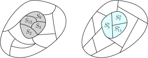
Figure 1: The blue set on the right, formed by $S_{5}^{*}\cup S_{7}^{*}\cup S_{11}^{*}$, conforms to the algorithm’s partition ${\cal S}$ on the left.

We now reduce the general $k$-Cut problem to Laminar $k$-cut. This reduction is again based on observations about the graph structure in cases where the iterative greedy algorithms do not get a $(2-\varepsilon$)-approximation. Suppose ${\cal S}=\{S_{1},\dots,S_{k^{\prime}}\}$ be the connected components of $G$ at some point of an iterative algorithm ($k^{\prime}\leq k$). For a subset $\emptyset\neq U\subsetneq V$, we say that $U$ conforms to partition ${\cal S}$ if there exists a subset $J\subsetneq[k^{\prime}]$ of parts such that $U=\cup_{j\in J}S_{j}$. One simple but crucial observation is the following: if there exists a subset $\emptyset\neq I\subsetneq[k]$ of indices such that $\cup_{i\in I}S^{*}_{i}$ conforms to ${\cal S}$ (i.e., $\cup_{i\in I}S^{*}_{i}=\cup_{j\in J}S_{j}$), we can “guess” $J$ to partition $V$ into the two parts $\cup_{i\in I}S^{*}_{i}$ and $\cup_{i\notin I}S^{*}_{i}$. Since the edges between these two parts belong to the optimal cut and each of them is strictly smaller than $V$, we can recursively work on each part without any loss.

Moreover, the number of choices for $J$ is at most $2^{k^{\prime}}$ and each guess produces one more connected component, so the total running time can be bounded by $f(k)$ times the running time of the rest of the algorithm, for some function $f(\cdot)$. Therefore, we can focus on the case where none of $\cup_{i\in I}S^{*}_{i}$ conforms to the algorithm’s partition ${\cal S}$ at any point during the algorithm’s execution.

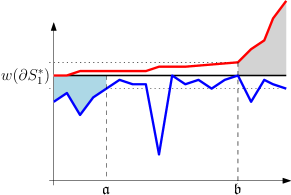
Figure 2: The blue curve shows cut sizes for algorithm’s cuts, red curve shows $w(\partial{S^{*}_{i}})$ values. The blue area (and in fact all the area below $w(\partial{S_{1}^{*}})$ and above the algorithm’s curve) makes the first inequality loose. The grey area (and in fact all the area above $w(\partial{S_{1}^{*}})$ and below OPT’s curve) makes the second inequality loose.

Now consider the iterative min-cut algorithm of Saran and Vazirani, and let $c_{i}$ be the cost of the min cut in the $i^{th}$ iteration ($1\leq i\leq k-1$). By our above assumption about non-conformity, none of $\cup_{i\in I}S^{*}_{i}$, and in particular the subset $S^{*}_{1}$, conform to the current components. This implies that deleting the remaining edges in $\partial S^{*}_{1}$ is a valid cut that increases the number of connected components by at least $1$, so $c_{i}\leq w(\partial{S^{*}_{1}})$. Then we have the following chain of inequalities:

$$\sum_{i=1}^{k-1}c_{i}\leq k\cdot w(\partial{S^{*}_{1}})\leq\sum_{i=1}^{k}w(\partial{S^{*}_{i}})=2\mathsf{Opt}.$$

If the iterative min-cut algorithm could not get a $(2-\varepsilon)$-approximation, the two inequalities above must be essentially tight. Hence almost all our costs $c_{i}$ must be close to $w(\partial{S^{*}_{1}})$ and almost all $w(\partial{S^{*}_{i}})$ must be close to $w(\partial{S^{*}_{1}})$. Slightly more formally, let $\mathfrak{a}\in[k]$ be the smallest integer such that $c_{\mathfrak{a}}\gtrsim w(\partial{S^{*}_{1}})$ —so that the first $\mathfrak{a}-1$ cuts are ones where we pay “much” less than $\partial{S^{*}_{1}}$ and make the first inequality loose. And let $\mathfrak{b}\in[k]$ be the smallest number such that $w(\partial{S^{*}_{\mathfrak{b}}})\gtrsim w(\partial{S^{*}_{1}})$ — so that the last $k-\mathfrak{b}$ cuts in OPT are much larger than $\partial{S^{*}_{1}}$ and make the second inequality loose. Then if the iterative min-cut algorithm is no better than a $2$-approximation, we can imagine that $\mathfrak{a}=o(k)$ and $\mathfrak{b}\geq k-o(k)$. For simplicity, let us assume that $\mathfrak{a}=1$ and $\mathfrak{b}=k$ here.

Indeed, instead of just considering min-cuts, suppose we also consider min-4-cuts, and take the one with better edges cut per number of new components. The arguments of the previous paragraph still hold, so $\mathfrak{a}=1$ implies that the best min-cuts and best min-4-way cuts (divided by 3) are roughly at least $w(\partial{S^{*}_{1}})$ in the original $G$. Since the min-cut is also at most $w(\partial{S^{*}_{1}})$, the weight of the min-cut is roughly $w(\partial{S^{*}_{1}})$ and none of the near-min-cuts cross (else we would get a good 4-way cut). I.e., the near-min-cuts in the graph form a laminar family. Together with the fact that $\partial{S^{*}_{1}},\dots,\partial{S^{*}_{k-1}}$ are near-min-cuts (we assumed $\mathfrak{b}=k$), this is precisely an instance of Laminar $k$-cut, which completes the proof!

Roadmap.

After some related work and preliminaries, we first present the details of the reduction from $k$-Cut to Laminar $k$-cut in Section 3. Then in Section 4 we give the algorithm for Laminar $k$-cut assuming an algorithm for Partial VC. Finally we give our FPT-AS for Partial VC in Section 5.

1.2 Other Related Work

The $k$-Cut problem has been widely studied. Goldschmidt and Hochbaum gave an $O(n^{(1/2-o(1))k^{2}})$-time algorithm [GH94]; they also showed that the problem is NP-hard when $k$ is part of the input. Karger and Stein improved this to an $O(n^{(2-o(1))k})$-time randomized Monte-Carlo algorithm using the idea of random edge-contractions [KS96]. After Kamidoi et al. [KYN07] gave an $O(n^{4k+o(1)})$-time deterministic algorithm based on divide-and-conquer, Thorup gave an $\tilde{O}(n^{2k})$-time deterministic algorithm based on tree packings [Tho08]. Small values of $k\in[2,6]$ also have been separately studied [NI92, HO94, BG97, Kar00, NI00, NKI00, Lev00].

On the approximation algorithms front, a $2(1-1/k)$-approximation was given by Saran and Vazirani [SV95]. Naor and Rabani [NR01], and Ravi and Sinha [RS08] later gave $2$-approximation algorithms using tree packing and network strength respectively. Xiao et al. [XCY11] completed the work of Kapoor [Kap96] and Zhao et al. [ZNI01] to generalize Saran and Vazirani to essentially give an $(2-h/k)$-approximation in time $n^{O(h)}$. Very recently, Manurangsi [Man17] showed that for any $\varepsilon>0$, it is NP-hard to achieve a $(2-\varepsilon)$-approximation algorithm in time $\mathrm{poly}(n,k)$ assuming the Small Set Expansion Hypothesis.

FPT algorithms: Kawarabayashi and Thorup give an $f(\mathsf{Opt})\cdot n^{2}$-time algorithm [KT11] for unweighted graphs. Chitnis et al. [CCH⁺16] used a randomized color-coding idea to give a better runtime, and to extend the algorithm to weighted graphs. In both cases, the FPT algorithm is parameterized by the cardinality of edges in the optimal $k$-Cut, not by $k$. For a comprehensive treatment of FPT algorithms, see the excellent book [CFK⁺15], and for a survey on approximation and FPT algorithms, see [Mar07].

Multiway Cut: A problem very similar to $k$-Cut is the Multiway Cut problem, where we are given $k$ terminals and want to disconnect the graph into at least $k$ pieces such that all terminals lie in distinct components. However, this problem behaves quite differently: it is NP-hard even for $k=3$ (and hence an $n^{f(k)}$ algorithm is ruled out); on the other hand several algorithms are known to approximate it to factors much smaller than $2$ (see, e.g., [BSW17] and references therein). FPT algorithms parameterized by the size of $\mathsf{Opt}$ are also known; see [CCF14] for the best result currently known.

2 Notation and Preliminaries

For a graph $G=(V,E)$, and a subset $S\subseteq V$, we use $G[S]$ to denote the subgraph induced by the vertex set $S$. For a collection of disjoint sets $S_{1},S_{2},\ldots,S_{t}$, let $E(S_{1},\ldots,S_{t})$ be the set of edges with endpoints in some $S_{i},S_{j}$ for $i\neq j$. Let $\partial S=E(S,V\setminus S)$. We say two cuts $(A,V\setminus A)$ and $(B,V\setminus B)$ cross if none of the four sets $A\setminus B,B\setminus A,A\cap B$, and $V\setminus(A\cup B)$ is empty. $\mathsf{Mincut}$ and Min-4-cut denote the weight of the min-2-cut and the min-4-cut respectively. A cut $(A,V\setminus A)$ is called $(1+\varepsilon)$-mincut if $w(A,V\setminus A)\leq(1+\varepsilon)\mathsf{Mincut}$.

Definition 2.1 (Laminar $k$-Cut$(\varepsilon_{1})$).

The input is a graph $G=(V,E)$ with edge weights, and two parameters $k$ and $\varepsilon_{1}$, satisfying two promises: (i) no two $(1+\varepsilon_{1})$-mincuts cross each other, and (ii) there exists a $k$-cut ${\cal S}^{\prime}=\{S_{1}^{\prime},\ldots,S_{k}^{\prime}\}$ in $G$ with $w(\partial(S_{i}^{\prime}))\leq(1+\varepsilon_{1})\mathsf{Mincut}(G)$ for all $i\in[1,k-1]$. Find a $k$-cut with the total weight. The approximation ratio is defined as the ratio of the weight of the returned cut to the weight of the $k$-Cut ${\cal S}^{\prime}$ (which can be possibly less than $1$).

Definition 2.2 (Minimum Partial Vertex Cover).

Given a graph $G=(V,E)$ with edge and vertex weights, and an integer $k$, find a vertex set $S\subseteq V$ with $|S|=k$ nodes, minimizing the weight of the edges hitting the set $S$ plus the weight of all vertices in $S$.

3 Reduction to $\textsc{Laminar }k\textsc{-cut}(\varepsilon_{1})$

In this section we give our reduction from $k$-Cut to $\textsc{Laminar }k\textsc{-cut}(\varepsilon_{1})$, showing that if we can get a better-than-2 approximation for the latter, we can beat the factor of two for the general $k$-Cut problem too. We assume the reader is familiar with the overview in Section 1.1.3. Formally, the main theorem is the following.

Theorem 3.1.

Suppose there exists a $(2-\varepsilon_{2})$-approximation algorithm for $\textsc{Laminar }k\textsc{-cut}(\varepsilon_{1})$ for some $\varepsilon_{1}\in(0,1/4)$ and $\varepsilon_{2}\in(0,1)$ that runs in time $f(k)\cdot g(n)$. Then there exists a $(2-\varepsilon_{3})$-approximation algorithm for $k$-Cut that runs in time $2^{O(k^{2}\log k)}\cdot f(k)\cdot(n^{4}\log^{3}n+g(n))$ for some constant $\varepsilon_{3}>0$.

Algorithm 1 $\text{Main}(G=(V,E,w),k)$

1:$k^{\prime}=1$, $S_{1}\leftarrow V$

2:while $k^{\prime}<k$  do

3:     for $\bm{\mathrm{r}}\in[k]^{k^{\prime}}$  do $\triangleright$ Further partition each $S_{i}$ into $r_{i}$ components by Laminar

4:         $|\bm{\mathrm{r}}|\leftarrow\sum_{j=1}^{k^{\prime}}r_{j}$; $\{C_{1},\dots,C_{|\bm{\mathrm{r}}|}\}\leftarrow\cup_{i\in[k^{\prime}]}\text{Laminar}(G[S_{i}],r_{i})$.

5:         if $|\bm{\mathrm{r}}|\geq k$ then $C_{k}\leftarrow C_{k}\cup\dots\cup C_{|\bm{\mathrm{r}}|}$

6:         else

7:              $\{C_{1},\dots,C_{k}\}\leftarrow\text{Complete}(G,k,C_{1},\dots,C_{|\bm{\mathrm{r}}|})$

8:         end if

9:         Record($\text{Guess}(\{C_{1},\dots,C_{k}\})$)

10:     end for

11:      $\triangleright$ Split some $S_{i}$ by a mincut or a min-4-cut

12:     if $k^{\prime}>k-3$ or $\min_{i\in[k^{\prime}]}\mathsf{Mincut}(G[S_{i}])\leq\min_{i\in[k^{\prime}]}\text{\sf{Min-4-cut}}(G[S_{i}])/3$ then

13:         $i\leftarrow\min_{i}\mathsf{Mincut}(G[S_{i}])$; $\{T_{1},T_{2}\}\leftarrow\text{Mincut}(G[S_{i}])$

14:         $S_{i}\leftarrow T_{1}$; $S_{k^{\prime}+1}\leftarrow T_{2}$; $c_{k^{\prime}}\leftarrow\mathsf{Mincut}(G[S_{i}])$; $k^{\prime}\leftarrow k^{\prime}+1$

15:     else

16:         $i\leftarrow\arg\min_{i}\text{\sf{Min-4-cut}}(G[S_{i}])$; $\{T_{1},\dots,T_{4}\}\leftarrow\text{Min-4-cut}(G[S_{i}])$; $S_{i}\leftarrow T_{1}$

17:         $S_{k^{\prime}+1},S_{k^{\prime}+2},S_{k^{\prime}+3}\leftarrow T_{2},T_{3},T_{4}$; $c_{k^{\prime}},c_{k^{\prime}+1},c_{k^{\prime}+2}\leftarrow\text{\sf{Min-4-cut}}(G[S_{i}])/3$; $k^{\prime}\leftarrow k^{\prime}+3$

18:     end if

19:end while

20:let ${\cal S}=\{S_{1},\ldots,S_{k}\}$ be the final reference $k$-partition.

21:Record($\text{Guess}(G,k,{\cal S})$)

22:Return the best recorded $k$-partition.

Algorithm 2 $\text{Complete}(G=(V,E,w),k,{\cal C}=\{C_{1},\ldots,C_{\ell}\})$

1:while $\ell<k$ do

2:     $i\leftarrow\min_{i\in[\ell]}\mathsf{Mincut}(G[C_{i}])$; $T_{1},T_{2}\leftarrow\text{Mincut}(G[C_{i}])$

3:     $C_{i}\leftarrow T_{1}$; $C_{\ell+1}\leftarrow T_{2}$; $\ell\leftarrow\ell+1$

4:end while

5:Return ${\cal C}:=\{C_{1},\dots,C_{k}\}$.

Algorithm 3 $\text{Guess}(G=(V,E,w),k,{\cal C}=\{C_{1},\dots,C_{k}\})$

1:Record($C_{1},\dots,C_{k}$) $\triangleright$ Returned partition no worse than starting partition

2:for $\emptyset\neq J\subsetneq[k]$  do

3:     for $k^{\prime}=1,2,\dots,k-1$  do

4:         $L\leftarrow\cup_{j\in J}C_{j}$; $R\leftarrow V\setminus L$ $\triangleright$ Divide $S_{i}$ into two groups, take union of each group

5:         $D_{1},\dots,D_{k^{\prime}}\leftarrow\text{Main}(G[L],k^{\prime})$ $\triangleright$ and recurse

6:         $D_{k^{\prime}+1},\dots,D_{k}\leftarrow\text{Main}(G[R],k-k^{\prime})$

7:         Record($D_{1},\dots,D_{k}$)

8:     end for

9:end for

10:Return the best recorded $k$-partition among all these guesses.

The main algorithm is shown in Algorithm 1 (“Main”). It maintains a “reference” partition ${\cal S}$, which is initially the trivial partition where all vertices are in the same part. At each point, it guesses how many pieces each part $S_{i}$ of this reference partition ${\cal S}$ should be split into using the “Laminar” procedure, and then extends this to a $k$-cut using greedy cuts if necessary (Lines 3–10). It then extends the reference partition by either taking the best min-cut or the best min-4-cut among all the parts (Lines 12–18).

Every time it has a $k$-partition, it guesses (using “Guess”) if the union of some of the parts equals some part of the optimal partition, and uses that to try get a better partition. If one of the guesses is right, we strictly increase the number of connected components by deleting edges in the optimal $k$-cut, so we can recursively solve the two smaller parts. If none of our guesses was right during the algorithm, our analysis in Section 3.1 shows that there exist values of $k^{\prime},\bm{\mathrm{r}}$ such that ${\cal C}=\{C_{1},\dots,C_{k}\}$ in Line 7, obtained from the reference partition ${\cal S}=\{S_{1},\dots,S_{k^{\prime}}\}$ by running Laminar($G[S_{i}],r_{i}$) for each $i\in[k^{\prime}]$ and using Complete if necessary to get $k$ components, beats the $2$-approximation. Finally, a couple words about each of the subroutines.

• Mincut$(G=(V,E,w))$ (resp. Min-4-cut$(G)$) returns the minimum $2$-cut (resp. $4$-cut) as a partition of $V$ into $2$ (resp. $4$) subsets.

• The subroutine “Laminar” returns a $(2-\varepsilon_{2})$-approximation for Laminar $k$-cut($\varepsilon_{1}$), using the algorithm from Theorem 4.1. Recall the definition of the problem in Definition 2.1.

• The operation “Record(${\cal P}$)” in Guess and Main takes a $k$-partition ${\cal P}$ and compares the weight of edges crossing this partition to the least-weight $k$-partition recorded thus far (within the current recursive call). If the current partition has less weight, it updates the best partition accordingly.

• Algorithm 2(“Complete”) is a simple algorithm that given an $\ell$-partition ${\cal P}$ for some $\ell\leq k$, outputs a $k$-partition by iteratively taking the mincut in the current graph.

• Algorithm 3(“Guess”), when given an $\ell$-partition ${\cal P}$ “guesses” if the vertices belonging to some parts of this partition $\{S_{j}\}_{j\in J}$ coincide with the union of some $k^{\prime}$ parts of the optimal partition. If so, we have made tangible progress: it recursively finds a small $k^{\prime}$-cut in the graph induced by $\cup_{j\in J}S_{j}$, and a small $k-k^{\prime}$ cut in the remaining graph. It returns the best of all these guesses.

3.1 The Approximation Factor

Lemma 3.2 (Approximation Factor).

$\text{Main}(G,k)$ achieves a $(2-\varepsilon_{3})$ approximation for some $\varepsilon_{3}>0$ that depends on $\varepsilon_{1},\varepsilon_{2}$ in Theorem 3.1.

Proof.

We prove the lemma by induction on $k$. The value of $\varepsilon_{3}$ will be determined later. The base case $k=1$ is trivial. Fix some value of $k$, and a graph $G$. Let ${\cal S}=\{S_{1},\dots,S_{k}\}$ be the final reference partition generated by the execution of $\text{Main}(G,k)$, and let $c_{1},\dots,c_{k-1}$ be the values associated with it. From the definition of the $c_{i}$’s in Procedure Main, $\sum_{i=1}^{k-1}c_{i}=w(E(S_{1},\dots,S_{k}))$. The $k$-partition returned by $\text{Main}(G,k)$ is no worse than this partition ${\cal S}$ (because of the update on line 21), and hence has cost at most $\sum_{i=1}^{k-1}c_{i}=w(E(S_{1},\dots,S_{k}))$. Let us fix an optimal $k$-cut ${\cal S}^{*}=\{S^{*}_{1},\dots,S^{*}_{k}\}$, and let $w(\partial{S^{*}_{1}})\leq\dots\leq w(\partial{S^{*}_{k}})$. Let $\mathsf{Opt}:=w(E(S^{*}_{1},\dots,S^{*}_{k}))=\sum_{i=1}^{k}w(\partial{S^{*}_{i}})/2$.

Definition 3.3 (Conformity).

For a subset $\emptyset\neq U\subsetneq V$, we say that $U$ conforms to partition ${\cal S}$ if there exists a subset $J\subsetneq[k]$ of parts such that $U=\cup_{j\in J}S_{j}$. (See Figure 1.)

The following claim shows that if there exists a subset $\emptyset\neq I\subsetneq[k]$ of indices such that $\cup_{i\in I}S^{*}_{i}$ conforms to ${\cal S}$, the induction hypothesis guarantees a $(2-\varepsilon_{3})$-approximation.

Claim 3.4.

Suppose there exists a subset $\emptyset\neq I\subsetneq[k]$ such that $\cup_{i\in I}S_{i}^{*}$ conforms to ${\cal S}$. Then $\text{Main}(G,k)$ achieves a $(2-\varepsilon_{3})$-approximation.

Proof.

Since $S^{*}_{I}:=\cup_{i\in I}S^{*}_{i}$ conforms to ${\cal S}$, during the run of $\text{Guess}(G,k,{\cal S})$ it will record the $k$-partition $(\text{Main}(G[S^{*}_{I}],|I|),\text{Main}(G[V\setminus S^{*}_{I}],k-|I|))$, and hence finally output a $k$-partition which cuts no more edges than this starting partition. By the induction hypothesis, $\text{Main}(G[S^{*}_{I}],|I|)$ gives a $|I|$-cut of $G[S^{*}_{I}]$ whose cost is at most $(2-\varepsilon_{3})$ times $w(E(S^{*}_{i})_{i\in I})$, and $\text{Main}(G[V\setminus S^{*}_{I}],k-|I|)$ outputs a $(k-|I|)$-cut of $G[V\setminus S^{*}_{I}]$ of cost at most $(2-\varepsilon_{3})$ times $w(E(S^{*}_{i})_{i\notin I})$. Thus, the value of the best $k$-partition returned by $\text{Main}(G,k)$ is at most

$$w(E(S^{*}_{I},V\setminus S^{*}_{I}))+(2-\varepsilon_{3})\left(w(E(S^{*}_{i})_{i\in I})+w(E(S^{*}_{i})_{i\notin I})\right)$$

$$\leq \ (2-\varepsilon_{3})w(E(S^{*}_{1},\dots,S^{*}_{k}))=(2-\varepsilon_{3})\mathsf{Opt}.\qed$$

Therefore, to prove Lemma 3.2, it suffices to assume that no collection of parts in $\mathsf{Opt}$ conforms to our partition at any point in the algorithm. I.e.,

(A1): for every subset $\emptyset\neq I\subsetneq[k]$, $\cup_{i\in I}S^{*}_{i}$ does not conform to ${\cal S}=\{S_{1},\dots,S_{k}\}$.

Next, we study how $\mathsf{Opt}$ is related to $w(\partial{S_{1}^{*}})$. Note that $\mathsf{Opt}\geq(k/2)\cdot w(\partial{S_{1}^{*}})$. The next claim shows that we can strictly improve the $2$-approximation if $\mathsf{Opt}$ is even slightly bigger than that.

Claim 3.5.

For every $i=1,\dots,k-1$, $c_{i}\leq w(\partial{S^{*}_{1}})$. Moreover, if $\mathsf{Opt}\geq(k-1)w(\partial{S_{1}^{*}})/(2-\varepsilon_{3})$, $\text{Main}(G,k)$ achieves a $(2-\varepsilon_{3})$-approximation.

Proof.

Consider the beginning of an arbitrary iteration of the while loop of $\text{Main}(G,k)$. Let $k^{\prime}$ and ${\cal S}^{\prime}=\{S_{1},\dots,S_{k^{\prime}}\}$ be the values at that iteration. By (A1), set $S_{1}^{*}$ does not conform to ${\cal S}^{\prime}$ (because ${\cal S}^{\prime}$ only gets subdivided as the algorithm proceeds, and $S_{1}^{*}$ does not conform to the final partition ${\cal S}$). So there exists some $i\in[k^{\prime}]$ such that $S_{i}$ intersects both $S^{*}_{1}$ and $V\setminus S^{*}_{1}$. If we consider $G[S_{i}]$ and its mincut,

$$\mathsf{Mincut}(G[S_{i}])\leq w(E(S_{i}\cap S^{*}_{1},S_{i}\setminus S^{*}_{1}))\leq w(\partial{S^{*}_{1}}).$$

Now the new $c_{j}$ values created in this iteration of the while loop are at most the smallest mincut value, so we have that each $c_{j}\leq w(\partial{S_{1}^{*}})$. Therefore,

$$w(E(S_{1},\dots,S_{k}))=\sum_{i=1}^{k-1}c_{i}\leq(k-1)\cdot w(\partial{S_{1}^{*}}),$$

and $\text{Main}(G,k)$ achieves a $(2-\varepsilon_{3})$-approximation if $(k-1)w(\partial{S^{*}_{1}})\leq(2-\varepsilon_{3})\mathsf{Opt}$. ∎

Consequently, it suffices to additionally assume that $\mathsf{Opt}$ is close to $(\nicefrac{{k}}{{2}})\,w(\partial{S^{*}_{1}})$. Formally,

(A2): $\mathsf{Opt}<w(\partial{S^{*}_{1}})\cdot\frac{k-1}{2-\varepsilon_{3}}$.

Recall that $\varepsilon_{1},\varepsilon_{2}>0$ are the parameters such that there is a $(2-\varepsilon_{2})$-approximation algorithm for $\textsc{Laminar }k\textsc{-cut}(\varepsilon_{1})$. Let $\mathfrak{a}\in[k]$ be the smallest integer such that $c_{\mathfrak{a}}>w(\partial{S^{*}_{1}})(1-\nicefrac{{\varepsilon_{1}}}{{3}})$ (set $\mathfrak{a}=k$ if there is no such integer). (See Figure 2.) In other words, $\mathfrak{a}$ is the value of $k^{\prime}$ in the while loop of $\text{Main}(G,k)$ when both $\min_{i}\mathsf{Mincut}(G[S_{i}])$ and $\min_{i}\text{\sf{Min-4-cut}}(G[S_{i}])/3$ are bigger than $w(\partial{S^{*}_{1}})(1-\nicefrac{{\varepsilon_{1}}}{{3}})$ for the first time. Let $\varepsilon_{4}>0$ be a constant satisfying

$$(2/3)\cdot\varepsilon_{1}\varepsilon_{4}\geq\varepsilon_{3}.$$ (1)

The next claim shows that we are done if $\mathfrak{a}$ is large.

Claim 3.6.

If $\mathfrak{a}\geq\varepsilon_{4}k$, $\text{Main}(G,k)$ achieves a $(2-\varepsilon_{3})$-approximation.

Proof.

If $\mathfrak{a}\geq\varepsilon_{4}k$, we have

$$\sum_{i=1}^{k-1}c_{i} \leq(\mathfrak{a}-1)(1-\nicefrac{{\varepsilon_{1}}}{{3}})\cdot w(\partial{S^{*}_{1}})+(k-\mathfrak{a})\cdot w(\partial{S^{*}_{1}})$$

$$\leq k\cdot w(\partial{S^{*}_{1}})\cdot(1-\nicefrac{{\varepsilon_{1}\varepsilon_{4}}}{{3}})\leq(2-(\nicefrac{{2}}{{3}})\varepsilon_{1}\varepsilon_{4})\mathsf{Opt}\leq(2-\varepsilon_{3})\mathsf{Opt}.\qed$$

Thus, we can assume that our algorithm finds very few cuts appreciably smaller than $w(\partial{S^{*}_{1}})$.

(A3): $\mathfrak{a}<\varepsilon_{4}k$.

Let $\mathfrak{b}\in[k]$ be the smallest number such that $w(\partial{S^{*}_{\mathfrak{b}}})>w(\partial{S^{*}_{1}})(1+\nicefrac{{\varepsilon_{1}}}{{3}})$; let it be $k$ if there is no such number. (Again, see Figure 2.) Observe that $\mathfrak{a}$ is defined based on our algorithm, whereas $\mathfrak{b}$ is defined based on the optimal solution. Let $\varepsilon_{5}>0$ be a constant satisfying:

$$\frac{1}{2-\varepsilon_{3}}\leq\frac{1+\nicefrac{{\varepsilon_{1}\varepsilon_{5}}}{{3}}}{2}~{}~{}~{}\Leftrightarrow~{}~{}~{}(1+\nicefrac{{\varepsilon_{1}\varepsilon_{5}}}{{3}})(2-\varepsilon_{3})\geq 2.$$ (2)

The next claim shows that $\mathfrak{b}$ should be close to $k$.

Claim 3.7.

$\mathfrak{b}\geq(1-\varepsilon_{5})k$.

Proof.

Suppose that $\mathfrak{b}<(1-\varepsilon_{5})k$. We have

$$\ \frac{k\cdot w(\partial{S^{*}_{1}})}{2-\varepsilon_{3}}\stackrel{{\scriptstyle\textbf{(A2)}}}{{>}}\mathsf{Opt}=\frac{1}{2}\sum_{i=1}^{k}w(\partial{S^{*}_{i}})$$

$$\geq \ \frac{w(\partial{S^{*}_{1}})}{2}\left((1-\varepsilon_{5})k+\varepsilon_{5}k(1+\varepsilon_{1}/3)\right)=\frac{k\cdot w(\partial{S^{*}_{1}})}{2}\left(1+\nicefrac{{\varepsilon_{1}\varepsilon_{5}}}{{3}}\right),$$

which contradicts (2). ∎

Therefore, we can also assume that very few cuts in $\mathsf{Opt}$ are appreciably larger than $w(\partial{S^{*}_{1}})$.

(A4): $\mathfrak{b}\geq(1-\varepsilon_{5})k$.

Constructing an Instance of Laminar Cut: In order to construct the instance for the problem, let $S^{*}_{\geq\mathfrak{b}}=\cup_{i=\mathfrak{b}}^{k}S^{*}_{i}$ be the union of these last few components from ${\cal S}^{*}$ which have “large” boundary. Consider the iteration of the while loop when $k^{\prime}=\mathfrak{a}$ and consider $S_{1},\dots,S_{\mathfrak{a}}$ in that iteration. By its definition, $c_{\mathfrak{a}}>w(\partial{S_{1}^{*}})(1-\nicefrac{{\varepsilon_{1}}}{{3}})$. Hence

$$\min_{i}\mathsf{Mincut}(G[S_{i}])>w(\partial{S_{1}^{*}})(1-\nicefrac{{\varepsilon_{1}}}{{3}}),$$ (3)

$$\min_{i}\text{\sf{Min-4-cut}}(G[S_{i}])>3w(\partial{S_{1}^{*}})(1-\nicefrac{{\varepsilon_{1}}}{{3}}).$$ (4)

In particular, (4) implies that no two near-min-cuts cross, since two crossing near-min-cuts will result in a $4$-cut of weight roughly at most $2w(\partial{S_{1}^{*}})$. However, we are not yet done, since we need to factor out the effects of the $\mathfrak{a}-1$ “small” cuts found by our algorithm. For this, we need one further idea.

Let $\bm{\mathrm{r}}=(r_{1},r_{2},\ldots,r_{\mathfrak{a}})\in[k]^{\mathfrak{a}}$ be such that $r_{i}$ is the number of sets $S^{*}_{1},\dots,S^{*}_{\mathfrak{b}-1},S^{*}_{\geq\mathfrak{b}}$ that intersect with $S_{i}$, and let $|\bm{\mathrm{r}}|:=\sum_{i=1}^{\mathfrak{a}}r_{i}$. If we consider the bipartite graph where the left vertices are the algorithm’s components $S_{1},\dots,S_{\mathfrak{a}}$, the right vertices are $S^{*}_{1},\dots,S^{*}_{\mathfrak{b}-1},S^{*}_{\geq\mathfrak{b}}$, and two sets have an edge if they intersect, then $|\bm{\mathrm{r}}|$ is the number of edges. Since there is no isolated vertex and the graph is connected (otherwise there would exist $\emptyset\neq I\subsetneq[k^{\prime}]$ and $\emptyset\neq J\subsetneq[k]$ with $\cup_{i\in I}S_{i}=\cup_{j\in J}S^{*}_{j}$ contradicting (A1)), the number of edges is $|\bm{\mathrm{r}}|\geq\mathfrak{a}+\mathfrak{b}-1$.

Claim 3.8.

For each $i$ with $r_{i}\geq 2$, the graph $G[S_{i}]$ satisfies the two promises of the problem $\textsc{Laminar }r_{i}\textsc{-cut}(\varepsilon_{1})$.

Proof.

Fix $i$ with $r_{i}\geq 2$. Let $J:=\{j\in[\mathfrak{b}-1]\mid S_{i}\cap S^{*}_{j}\neq\emptyset\}$ be the sets $S_{j}^{*}$ among the first $\mathfrak{b}-1$ sets in the optimal partition that intersect $S_{i}$. Since $|J|\geq r_{i}-1$ and $r_{i}\geq 2$, $|J|\geq 1$. Note that $(1-\nicefrac{{\varepsilon_{1}}}{{3}})\cdot w(\partial{S^{*}_{1}})<\mathsf{Mincut}(G[S_{i}])$ by (3). For every $j\in J$,

$$\mathsf{Mincut}(G[S_{i}])\leq w(E(S_{i}\cap S^{*}_{j},S_{i}\setminus S^{*}_{j}))\leq w(\partial{S^{*}_{j}})\leq(1+\varepsilon_{1}/3)\;w(\partial{S^{*}_{1}})\leq(1+\varepsilon_{1})\;\mathsf{Mincut}(G[S_{i}]).$$

The first and second inequality hold since both parts $S_{i}\cap S^{*}_{j}$ and $S_{i}\setminus S^{*}_{j}$ are nonempty, and hence deleting all the edges in $\partial{S_{j}^{*}}$ would separate $G[S_{i}]$. The third inequality is by the choice of $\mathfrak{b}$, and the last inequality uses (3) and the fact that $(1+\nicefrac{{\varepsilon_{1}}}{{3}})\leq(1+\varepsilon_{1})(1-\nicefrac{{\varepsilon_{1}}}{{3}})$ when $\varepsilon_{1}<1/4$.

This implies that in $G[S_{i}]$, for every $j\in J$, $(S_{i}\cap S^{*}_{j},S_{i}\setminus S^{*}_{j})$ is a $(1+\varepsilon_{1})$-mincut. Furthermore, in $G[S_{i}]$, no two $(1+\varepsilon_{1})$-mincuts cross because it will result a 4-cut of cost at most

$$2(1+\varepsilon_{1})\;\mathsf{Mincut}(G[S_{i}])\leq 2(1+\varepsilon_{1})(1+\varepsilon_{1}/3)\;w(\partial{S_{1}^{*}}),$$

contradicting (4). (Note that $2(1+\varepsilon_{1})(1+\nicefrac{{\varepsilon_{1}}}{{3}})\leq 3(1-\nicefrac{{\varepsilon_{1}}}{{3}})$ when $\varepsilon_{1}<1/4$.) Hence, in $G[S_{i}]$, the two promises for $\textsc{Laminar }r_{i}\textsc{-cut}(\varepsilon_{1})$ are satisfied. ∎

Our algorithm $\text{Main}(G,k$) runs $\text{Laminar}(G[S_{i}],r_{i})$ for each $i\in[\mathfrak{a}]$ when it sets $k^{\prime}=\mathfrak{a}$ and the vector $\bm{\mathrm{r}}$ as defined above. As in the algorithm, let ${\cal C}=\{C_{1},\dots,C_{k}\}$ be the partition obtained in Line 7. In other words, to obtain the $k$ sets $C_{1},\dots,C_{k}$ from the set $V$, we take the reference partition $S_{1},\dots,S_{\mathfrak{a}}$ and further partition these sets using Laminar to get $|\bm{\mathrm{r}}|$ parts $C_{1},\dots,C_{|\bm{\mathrm{r}}|}$. If $|\bm{\mathrm{r}}|\geq k$, we can merge the last $|\bm{\mathrm{r}}|-k+1$ parts to get exactly $k$ parts if we want (but we will not take any edge savings into account in this calculation). If $|\bm{\mathrm{r}}|<k$, we get $k-|\bm{\mathrm{r}}|$ more parts using the Complete procedure.

The total cost of this solution ${\cal C}$ is $w(E(C_{1},\dots,C_{k}))$, which is $\sum_{j=1}^{\mathfrak{a}-1}c_{j}\leq(\mathfrak{a}-1)w(\partial{S^{*}_{1}})$ plus the cost of $\text{Laminar}(G[S_{i}],r_{i})$ for all $i\in[\mathfrak{a}]$ and the cost of Complete. Since Claim 3.8 considers the partition of each $G[S_{i}]$ obtained by cutting edges belonging to the optimal $k$-partition, the sum of the cost of the $r_{i}$-partition we compare to in each Laminar $r_{i}$-cut is exactly $\mathsf{Opt}$. Hence the cost of the solution given by $\text{Laminar}(G[S_{i}],r_{i})$ summed over $i\in[\mathfrak{a}]$ is bounded by $(2-\varepsilon_{2})\mathsf{Opt}$, by the approximation assumption in Theorem 3.1.

If $\cup_{i\in I}S^{*}_{i}$ for some $\emptyset\neq I\subsetneq[k]$ conforms to ${\cal C}$, then since Main also records $\text{Guess}({\cal C})$, the proof of Claim 3.4 guarantees that $\text{Main}(G,k)$ gives a $(2-\varepsilon_{3})$ approximation using the induction hypothesis. Otherwise, $S^{*}_{1}$ does not conform to ${\cal C}$, so the arguments used in the proof of Claim 3.5 show that the cost of Complete is at most $(k-|\bm{\mathrm{r}}|)\,w(\partial{S^{*}_{1}})$ if $|\bm{\mathrm{r}}|\leq k$, and $0$ otherwise. Since $|\bm{\mathrm{r}}|\geq\mathfrak{a}+\mathfrak{b}-1$, the total cost $w(E(C_{1},\dots,C_{k}))$ is then bounded by

$$(\mathfrak{a}-1)w(\partial{S^{*}_{1}})+(2-\varepsilon_{2})\mathsf{Opt}+(k-\mathfrak{a}-\mathfrak{b}+1)w(\partial{S^{*}_{1}})$$

$$= \ (2-\varepsilon_{2})\mathsf{Opt}+(k-\mathfrak{b})w(\partial{S^{*}_{1}})$$

$$\leq \ (2-\varepsilon_{2})\mathsf{Opt}+\varepsilon_{5}k\cdot w(\partial{S^{*}_{1}})$$ (by (A4))

$$\leq \ (2-\varepsilon_{2}+2\varepsilon_{5})\mathsf{Opt}.$$

Therefore, if

$$\varepsilon_{3}\leq\varepsilon_{2}-2\varepsilon_{5},$$ (5)

then $\text{Main}(G,k)$ gives a $(2-\varepsilon_{3})$ approximation in every possible case. We set $\varepsilon_{3},\varepsilon_{4},\varepsilon_{5}>0$ so that they satisfy the three conditions (1), (2), and (5), namely,

$$(2/3)\cdot\varepsilon_{1}\varepsilon_{4}\geq\varepsilon_{3},\quad(1+\varepsilon_{1}\varepsilon_{5}/3)(2-\varepsilon_{3})\geq 2,\quad\varepsilon_{3}\leq\varepsilon_{2}-2\varepsilon_{5}.$$

(For instance, setting $\varepsilon_{4}=\varepsilon_{5}=\min(\varepsilon_{1},\varepsilon_{2})/3$ and $\varepsilon_{3}=\varepsilon_{4}^{2}$ works.) ∎

3.2 Running Time

We prove that this algorithm also runs in FPT time, finishing the proof of Theorem 3.1.

Lemma 3.9.

Suppose that $\text{Laminar}(G,k)$ runs in time $f(k)\cdot g(n)$. Then Main$(G,k)$ runs in time $2^{O(k^{2}\log k)}\cdot f(k)\cdot(g(n)+n^{4}\log^{3}n)$.

Proof.

Let $\mathsf{Time}(\text{P})$ denote the running time of a procedure P. Here each procedure is only parameterized by the number of sets it outputs (e.g., $\text{Main}(k),\text{Guess}(k),\text{Complete}(k),\text{Laminar}(k)$). We use the fact that the global min-cut can be computed in time $O(n^{2}\log^{3}n)$ [KS96] and the min-$4$-cut can be computed in $O(n^{4}\log^{3}n)$ [Lev00]. First, $\mathsf{Time}(\text{Complete}(k))=O(kn^{2}\log^{3}n)$. For Guess and Main,

$$\mathsf{Time}(\text{Guess}(k))\leq k\cdot 2^{k+1}\cdot(\mathsf{Time}(\text{Main}(k-1))+O(n)),$$

and

$$\mathsf{Time}(\text{Main}(k)) \leq k^{k}\cdot(\mathsf{Time}(\text{Laminar}(k))+\mathsf{Time}(\text{Guess}(k))+\mathsf{Time}(\text{Complete}(k)))+O(kn^{4}\log^{3}n)$$

$$\leq 2^{O(k\log k)}\cdot f(k)\cdot(g(n)+O(n^{4}\log^{3}n))+2^{O(k\log k)}\cdot\mathsf{Time}(\text{Main}(k-1)).$$

We can conclude $\mathsf{Time}(\text{Main}(k))\leq 2^{O(k^{2}\log k)}\cdot f(k)\cdot(g(n)+n^{4}\log^{3}n)$. ∎

4 An Algorithm for Laminar $k$-cut

Recall the definition of the Laminar $k$-cut problem: See 2.1

Let $\mathcal{O}_{\varepsilon_{1}}$ contain all partitions $S_{1},\ldots,S_{k}$ of $V$ with the restriction that the boundaries of the first $k-1$ parts is small—i.e., $w(\partial{S_{i}})\leq(1+\varepsilon_{1})\mathsf{Mincut}(G)$ for all $i\in[k-1]$. We emphasize that the weight of the last cut, i.e., $w(\partial{S_{k}})$, is unconstrained. In this section, we give an algorithm to find a $k$-partition (possibly not in $\mathcal{O}_{\varepsilon_{1}}$) with total weight

$$w(E(S_{1},\ldots,S_{k}))\leq(2-\varepsilon_{2})\min\limits_{\{S_{i}^{\prime}\}\in\mathcal{O}_{\varepsilon_{1}}}w(E(S_{1}^{\prime},\ldots,S_{k}^{\prime})).$$

Formally, the main theorem of this section is the following:

Theorem 4.1 (Laminar Cut Algorithm).

Suppose there exists a $(1+\delta)$-approximation algorithm for $\textsc{Partial }k\textsc{-VC}$ for some $\delta\in(0,1/24)$ that runs in time $f(k)\cdot g(n)$. Then, for any $\varepsilon_{1}\in(0,1/6-4\delta)$, there exists a $(2-\varepsilon_{2})$-approximation algorithm for $\textsc{Laminar }k\textsc{-cut}(\varepsilon_{1})$ that runs in time $2^{O(k)}f(k)(\tilde{O}(n^{4})+g(n))$ for some constant $\varepsilon_{2}>0$.

In the rest of this section we present the algorithm and the analysis. For a formal description, see the pseudocode in Appendix A.

4.1 Mincut Tree

The first idea in the algorithm is to consider the structure of a laminar family of cuts. Below, we introduce the concept of a mincut tree. The vertices of the mincut tree are called nodes, to distinguish them from the vertices of the original graph.

Definition 4.2 (Mincut Tree).

A tree $\mathcal{T}=(V_{\mathcal{T}},E_{\mathcal{T}},w_{\mathcal{T}})$ is a $(1+\varepsilon_{1})$-mincut tree on a graph $G=(V,E,w)$ with mapping $\phi:V\to V_{\mathcal{T}}$ if the following two sets are equivalent:

1. The set of all $(1+\varepsilon_{1})$-mincuts of $G$.

2. Cut a single edge $e\in E_{\mathcal{T}}$ of the tree, and let $A_{e}\subset V_{\mathcal{T}}$ be the nodes on one side of the cut. Define $S_{e}:=\phi^{-1}(A_{e})=\{v\mid\phi(v)\in A_{e}\}$ for each $e\in E_{\mathcal{T}}$, and take the set of cuts $\{(S_{e},V\setminus S_{e}):e\in E_{\mathcal{T}}\}$.

Moreover, for every pair of corresponding $(1+\varepsilon_{1})$-mincut $(S_{e},V\setminus S_{e})$ and edge $e\in E_{\mathcal{T}}$, we have $w_{\mathcal{T}}(e)=w(E(S_{e},V\setminus S_{e}))$.

We use the term mincut tree without the $(1+\varepsilon_{1})$ when the value of $\varepsilon_{1}$ is either implicit or irrelevant.

For the rest of this section, let

$${\mu}:=\mathsf{Mincut}(G)$$

for brevity. Observe that the last condition implies that ${\mu}\leq w_{\mathcal{T}}(e)\leq(1+\varepsilon_{1}){\mu}$ for all $e\in E_{\mathcal{T}}$. The existence of a mincut tree (and the algorithm for it) assuming laminarity, is standard, going back at least to Edmonds and Giles [EG77].

Theorem 4.3 (Mincut Tree Existence/Construction).

If the set of $(1+\varepsilon_{1})$-mincuts of a graph is laminar, then an $O(n)$-sized $(1+\varepsilon_{1})$-mincut tree always exists, and can be found in $O(n^{3})$ time.

Proof.

We refer the reader to [KV12, Section 2.2]. Fix a vertex $v\in V$, and for each $(1+\varepsilon_{1})$-mincut $(S,V\setminus S)$, pick the side that contains $v$; this family of subsets of $V$ satisfies the laminar condition in Proposition 2.12 of that book. Corollary 2.15 proves that this family has size $O(n)$, and the construction of $T$ in Proposition 2.14 gives the desired mincut tree. Furthermore, we can compute the mincut tree in $O(n^{3})$ time as follows: first precompute whether $X\subset Y$ for every two sets $X$ and $Y$ in the family, and then compute $T$ following the construction in the proof of Proposition 2.14. ∎

Definition 4.4 (Mincut Tree Terminology).

Let $\mathcal{T}$ be a rooted mincut tree. For $a\in V_{\mathcal{T}}$, define the following terms:

• $\mathrm{children}(a)$: the set of children of node $a$ in the rooted tree.

• $\mathrm{desc}(a)$: the set of descendants of $a$, i.e., nodes $b\in V_{\mathcal{T}}\setminus a$ whose path to the root includes $a$.

• $\mathrm{anc}(a)$: the set of ancestors of $a$, i.e., nodes $b\in V_{\mathcal{T}}\setminus a$ on the path from $a$ to the root.

• $\mathrm{subtree}(a)$: vertices in the subtree rooted at $a$, i.e., $\{a\}\cup\mathrm{desc}(a)$.

For the set of partitions $\mathcal{O}_{\varepsilon_{1}}$ (as defined at the beginning of this section), we observe the following.

Claim 4.5 (Representing Laminar Cuts in $\mathcal{T}$).

Let $\mathcal{T}=(V_{\mathcal{T}},E_{\mathcal{T}},w_{\mathcal{T}})$ be a $(1+\varepsilon_{1})$-mincut tree of $G=(V,E,w)$, and consider a partition $\{S_{1},\ldots,S_{k}\}\in\mathcal{O}_{\varepsilon_{1}}$. Then, there exists a root $r\in V_{\mathcal{T}}$ and nodes $a_{1},\ldots,a_{k-1}\in V_{\mathcal{T}}\setminus r$ such that if we root the tree $\mathcal{T}$ at $r$,

1. For any two nodes in $\{a_{1},\ldots,a_{k-1}\}$, neither is an ancestor of the other. (We call two such nodes incomparable).

2. For each $v_{i}$, let $A_{i}:=\mathrm{subtree}(a_{i})$, and let $A_{k}=V_{\mathcal{T}}\setminus\bigcup_{i=1}^{k-1}A_{i}$ (so that $r\in A_{k}$). We have the two equivalences $\{\phi^{-1}(A_{i})\mid i\in[k-1]\}=\{S_{1},\ldots,S_{k-1}\}$ and $\phi^{-1}(A_{k})=S_{k}$. In other words, the components $A_{i}\subset V_{\mathcal{T}}$, when mapped back by $\phi^{-1}$, correspond exactly to the sets $S_{i}\subset V$, with the additional guarantee that $A_{k}$ and $S_{k}$ match.

Proof.

Since $S_{i}$ is a $(1+\varepsilon_{1})$-mincut for each $i\in[k-1]$, there exists an edge $e_{i}\in E_{\mathcal{T}}$ such that the set $A_{i}^{\prime}$ of nodes on one side of $e_{i}$ satisfies $\phi^{-1}(A_{i}^{\prime})=S_{i}$. The sets $A_{i}^{\prime}$ for $i\in[k-1]$ are necessarily disjoint, and they cannot span all nodes in $V_{\mathcal{T}}$, since $S_{k}$ is still unaccounted for. If we root $\mathcal{T}$ at a node $r$ not in any $A_{i}^{\prime}$, then each $A_{i}^{\prime}$ is a subtree of the rooted $\mathcal{T}$. Altogether, the roots of the subtrees $A_{i}^{\prime}$ satisfy condition (1) of the lemma, and the $A_{i}^{\prime}$ themselves satisfy condition (2). ∎

For a graph $G=(V,E,w)$ and mincut tree $\mathcal{T}=(V_{\mathcal{T}},E_{\mathcal{T}},w_{\mathcal{T}})$ with mapping $\phi:V\to V_{\mathcal{T}}$, define $E_{G}(A,B)$ for $A,B\subset V_{\mathcal{T}}$ as $E\left(\phi^{-1}(A),\phi^{-1}(B)\right)$, i.e., the total weight of edges crossing the sets corresponding to $A$ and $B$ in $V$.

Observation 4.6.

Given a root $r\in V_{\mathcal{T}}$ and incomparable nodes $a_{1},\ldots,a_{k-1}\in V_{\mathcal{T}}\setminus r$, we can bound the corresponding partition $S_{1},\ldots,S_{k}$ as follows:

$$w(E(S_{1},\ldots,S_{k})) =\textstyle\sum_{i=1}^{k-1}w(\partial(S_{i}))-\sum_{i<j\leq k-1}w(E(S_{i},S_{j}))$$

$$=\textstyle\sum_{i=1}^{k-1}w_{\mathcal{T}}(e_{i})-\sum_{i<j\leq k-1}w(E_{G}(\mathrm{subtree}(a_{i}),\mathrm{subtree}(a_{j}))),$$

where $e_{i}$ is the parent edge of $v_{i}$ in the rooted tree.

Note that ${\mu}\leq w_{\mathcal{T}}(e)\leq(1+\varepsilon_{1}){\mu}$ for all $e\in E_{\mathcal{T}}$, so to approximately minimize the above expression for a fixed root $r$, it suffices to approximately maximize

$$\textstyle\mathsf{Saved}(a_{1},\ldots,a_{k-1}):=\sum\limits_{i<j\leq k-1}w(E_{G}(\mathrm{subtree}(a_{i}),\mathrm{subtree}(a_{j}))),$$

which we think of as the edges saved in the double counting of $\sum_{i=1}^{k-1}w_{\mathcal{T}}(e_{i})$. The actual approximation factor is made precise in the proof of Theorem 4.1.

To maximize the number of saved edges over all partitions in $\mathcal{O}_{\varepsilon_{1}}$, it suffices to try all possible roots $r$ and take the best partition. Therefore, for the rest of this section, we focus on maximizing $\mathsf{Saved}(a_{1},\ldots,a_{k-1})$ for a fixed root $r$. Let $\ell^{*}(r)$ be that maximum value for root $r$, and let $\mathsf{Opt}(r)=\{a_{1}^{*},\ldots,a_{k-1}^{*}\}\subset V_{\mathcal{T}}$ be the solution that attains it.

4.2 Anchors

Root the mincut tree $\mathcal{T}$ at $r$, and let $a_{1}^{*},\ldots,a_{k-1}^{*}$ be incomparable nodes in the solution $\mathsf{Opt}(r)$. First, observe that we can assume w.l.o.g. that for each node $a_{i}^{*}$, its parent node is an ancestor of some $a_{j}^{*}\neq a_{i}^{*}$: if not, we can replace $a_{i}^{*}$ with its parent, which can only increase $\mathsf{Saved}(a_{1}^{*},\ldots,a_{k-1}^{*})$.

Observation 4.7.

Consider nodes $a_{1}^{*},\ldots,a_{s}^{*}\in\mathsf{Opt}(r)$ which share the same parent $a\notin\mathsf{Opt}(r)$, and assume that $a$ has no other descendants. If we replace $a_{1}^{*},\ldots,a_{s}^{*}$ in $\mathsf{Opt}(r)$ with $a$, then we lose at most $\mathsf{Saved}(a_{1}^{*},\ldots,a_{s}^{*})$ in our solution.

If $\mathsf{Saved}(a_{1}^{*},\ldots,a_{s}^{*})$ is small, i.e., compared to $(s-1){\mu}$, then we do not lose too much. This idea motivates the idea of anchors.

Definition 4.8 (Anchors).

Let $\mathcal{T}=(V_{\mathcal{T}},E_{\mathcal{T}},w_{\mathcal{T}})$ be a rooted tree. For a fixed constant $\varepsilon_{3}>0$, define an $\varepsilon_{3}$-anchor to be a node $a\in V_{\mathcal{T}}$ such that there exists $s\in[2,k-1]$ and $s$ children $a_{1},\ldots,a_{s}$ such that $\mathsf{Saved}(a_{1},\ldots,a_{s})\geq\varepsilon_{3}(s-1){\mu}$. When the value of $\varepsilon_{3}$ is implicit, we use the term anchor, without the $\varepsilon_{3}$.

We now claim that we can transform any solution to another well-structured solution, with only a minimal loss.

Lemma 4.9 (Shifting Lemma).

Let $a_{1},\ldots,a_{k-1}$ be a set of incomparable nodes of a $(1+\varepsilon_{1})$-mincut tree $\mathcal{T}$. Then, there exists a set $b_{1},\ldots,b_{s}$ of incomparable nodes, for $1\leq s\leq k-1$, such that

1. The parent of every node $b_{i}$ is either an $\varepsilon_{3}$-anchor, or is an ancestor of some node $b_{j}\neq b_{i}$ whose parent is an anchor.

2. $\mathsf{Saved}(b_{1},\ldots,b_{s})\geq\mathsf{Saved}(a_{1},\ldots,a_{k-1})-\varepsilon_{3}(k-s){\mu}$.

In particular, if $\{a_{1},\ldots,a_{k-1}\}=\mathsf{Opt}(r)$, condition (2) implies $\mathsf{Saved}(b_{1},\ldots,b_{s})\geq\ell^{*}(r)-\varepsilon_{3}(k-1){\mu}$.

Proof.

We begin with the solution $b_{i}=a_{i}$ for all $i$, and iteratively shift non-anchors in the solution while maintaining the potential function $\Phi:=\mathsf{Saved}(b_{1},\ldots,b_{s})-\mathsf{Saved}(a_{1},\ldots,a_{k-1})+\varepsilon_{3}(k-s){\mu}$ nonnegative. At the beginning, $\Phi=0$. Suppose there is a node $b_{i}$ not satisfying condition (1). Choose one such $b_{i}$ of maximum depth in the tree, and let $b^{\prime}$ be its non-anchor parent. Then the only descendants of $b^{\prime}$ in the current solution are siblings of $b_{i}$. Replace $b_{i}$ and its $s^{\prime}$ siblings in the solution by $b^{\prime}$. Since $b^{\prime}$ is not an anchor, $\mathsf{Saved}(b_{1},\ldots,b_{s})$ drops by at most $\varepsilon_{3}(s^{\prime}-1){\mu}$. This drop is compensated by the decrease of the solution size from $s$ to $s-(s^{\prime}-1)$. ∎

Hence, at a loss of $\varepsilon_{3}(k-1){\mu}$, it suffices to focus on a solution $\mathsf{Opt}^{\prime}(r)$ which fulfills condition (1) of Lemma 4.9 and has $\mathsf{Saved}$ value $\ell^{\prime}(r)\geq\ell^{*}(r)-\varepsilon_{3}(k-1){\mu}$.

The rest of the algorithm splits into two cases. At a high level, if there are enough anchors in a mincut tree $\mathcal{T}$ that are incomparable with each other, then we can take such a set and be done. Otherwise, the set of anchors can be grouped into a small number of paths in $\mathcal{T}$, and we can afford to try all possible arrangements of anchors. But first we show how to find all the anchors in $\mathcal{T}$.

4.3 Finding Near-Anchors

Lemma 4.10 (Finding (Near-)Anchors).

Assume access to a $(1+\delta)$-approximation algorithm for $\textsc{Partial }k\textsc{-VC}$ running in time $f(k)\cdot g(n)$. Then, there is an algorithm running in time $O(n\cdot(n^{2}+k\cdot f(k)\cdot g(n)))$ that computes a set $\mathcal{A}$ of “near”-anchors in $\mathcal{T}$, i.e., vertices $a\in V_{\mathcal{T}}$ for which there exists an integer $s\in[2,k-1]$ and $s$ children $b_{1},\ldots,b_{s}$ such that $\mathsf{Saved}(b_{1},\ldots,b_{s})\geq\varepsilon_{3}(s-1){\mu}-\delta(1+\varepsilon_{1})s{\mu}$.

Proof.

To determine if a node $a$ is an anchor or not, for each integer $s\in[2,k-1]$ we wish to compute the maximum value of $\mathsf{Saved}(b_{1},\ldots,b_{s})$ for $b_{1},\ldots,b_{s}\in\mathrm{children}(a)$. Consider the following weighted, complete graph with vertex and edge weights: for each $b\in\mathrm{children}(a)$ create a vertex $x_{b}$, and the edge $(x_{b_{1}},x_{b_{2}})$ has weight $\mathsf{Saved}(b_{1},b_{2})$. Each vertex $x_{b}$ also has weight $(1+\varepsilon_{1}){\mu}-w(\partial x_{b})$, where $w(\partial x_{b})$ is the sum of the weights of edges incident to $x_{b}$. Note that this graph is $(1+\varepsilon_{1}){\mu}$-regular, if we include vertex weights in the definition of vertex degree.

Observe that $w(\partial x_{b})\leq\partial\left(\phi^{-1}(\mathrm{subtree}(b))\right)\leq(1+\varepsilon_{1}){\mu}$, since every edge in $G$ that contributes to $\mathsf{Saved}(b,b^{\prime})$ for another child $b^{\prime}$ also contributes to the cut $\partial\left(\phi^{-1}(\mathrm{subtree}(b))\right)$, which we know is $\leq(1+\varepsilon_{1}){\mu}$. Therefore, each vertex has a nonnegative weight. Also, a partial vertex cover on this graph with vertices $x_{b_{1}},\ldots,x_{b_{s}}$ has weight exactly $(1+\varepsilon_{1})s{\mu}-\mathsf{Saved}(b_{1},\ldots,b_{s})$.

Let $b_{1}^{*},\ldots,b_{s}^{*}\in\mathrm{children}(a)$ be the solution with maximum $\mathsf{Saved}(b_{1}^{*},\ldots,b_{s}^{*})$. To compute this maximum, we can build the above graph and run the $(1+\delta)$-approximate partial vertex cover algorithm from Theorem 5.1. The solution $b_{1},\ldots,b_{s}$ satisfies

$$(1+\varepsilon_{1})s{\mu}-\mathsf{Saved}(b_{1},\ldots,b_{s})\leq(1+\delta)\left((1+\varepsilon_{1})s{\mu}-\mathsf{Saved}(b_{1}^{*},\ldots,b_{s}^{*})\right),$$

so that

$$\mathsf{Saved}(b_{1},\ldots,b_{s}) \geq(1+\delta)\,\mathsf{Saved}(b_{1}^{*},\ldots,b_{s}^{*})-\delta(1+\varepsilon_{1})s{\mu}$$

$$\geq\mathsf{Saved}(b_{1}^{*},\ldots,b_{s}^{*})-\delta(1+\varepsilon_{1})s{\mu}.$$

We run this subprocedure for the vertex $a$ for each integer $2\leq s\leq\min\{|\mathrm{children}(a)|,k-1\}$, and mark vertex $a$ if there exists an integer $s$ such that the weight of saved edges is at least $\varepsilon_{3}(s-1){\mu}-\delta(1+\varepsilon_{1})s{\mu}$. The set $\mathcal{A}$ of near-anchors is exactly the set of marked vertices.

As for running time, for each node $a$, it takes $O(n^{2})$ time to construct the Partial VC graph and $O(k)\cdot f(k)\cdot g(n)$ time to solve $\textsc{Partial }s\textsc{-VC}$ for each $s\in[2,k-1]$. Repeating the above for each of the $O(n)$ nodes achieves the promised running time. ∎

4.4 Many Incomparable Near-Anchors

Lemma 4.11 (Many Anchors).

Suppose we have access to a $(1+\delta)$-approximation algorithm for $\textsc{Partial }k\textsc{-VC}$ running in time $f(k)\cdot g(n)$. Suppose the set $\mathcal{A}$ of near-anchors contains $k-1$ incomparable nodes from the mincut tree $\mathcal{T}$. Then, there is an algorithm computing a solution with $\mathsf{Saved}$ value $\geq\frac{1}{4}\varepsilon_{3}(k-1){\mu}-\delta(1+\varepsilon_{1})(k-1){\mu}$ for any $\delta>0$, running in time $O(n\cdot(n^{2}+k\cdot f(k)\cdot g(n)))$.

Proof.

First, we compute the set $\mathcal{A}$ in $O(n\cdot(n^{2}+k\cdot f(k)\cdot g(n))$ time, according to Lemma 4.10. If $\mathcal{A}$ contains $k-1$ incomparable nodes, we can find them in $O(n^{2})$ time by greedily choosing nodes in a topological, bottom-first order (see lines 4–11 in Algorithm 7). Each of these $k-1$ marked nodes $a_{1},\ldots,a_{k-1}$ has an associated value $s_{i}$, indicating that $a_{i}$ has some $s_{i}$ children whose $\mathsf{Saved}$ value is at least $\varepsilon_{3}(s_{i}-1){\mu}-\delta(1+\varepsilon_{1})s_{i}{\mu}$. If we consider a subset $A\subset[k-1]$ and choose the $s_{i}$ children for each $a_{i}$ with $i\in A$, then we get a set with $\sum_{i\in A}s_{i}$ nodes, whose total $\mathsf{Saved}$ value at least

$$\varepsilon_{3}\left(\sum_{i\in A}(s_{i}-1)\right){\mu}-\delta(1+\varepsilon_{1})\left(\sum_{i\in A}s_{i}\right){\mu}.$$

Assuming that $\sum_{i\in A}s_{i}\leq k-1$, i.e., we choose at most $k-1$ children, the second $\delta(1+\varepsilon_{1})\left(\sum_{i\in A}s_{i}\right){\mu}$ term is at most $\delta(1+\varepsilon_{1})(k-1){\mu}$. To optimize the $\varepsilon_{3}\left(\sum_{i\in A}(s_{i}-1)\right){\mu}$ term, we reduce to the following knapsack problem: we have $k-1$ items $i\in[k-1]$ where item $i$ has size $s_{i}\in[2,k-1]$ and value $s_{i}-1$, and our bag size is $k-1$. A knapsack solution of value $Z:=\sum_{i\in A}(s_{i}-1)$ translates to a solution with $\mathsf{Saved}$ value $\geq\varepsilon_{3}{\mu}\cdot Z-\delta(1+\varepsilon_{1})(k-1){\mu}$. By Lemma B.1, when $k\geq 5$, we can compute a solution $A\subset[k-1]$ of value $\geq(k-1)/4$ in $O(k)$ time. (If $k\leq 4$, we can use the exact $\tilde{O}(n^{4})$ $k$-Cut algorithm from [Lev00].) Selecting the children of each $u_{i}$ with $i\in A$ gives a total $\mathsf{Saved}$ value of at least $\frac{1}{4}\varepsilon_{3}(k-1){\mu}-\delta(1+\varepsilon_{1})(k-1){\mu}$. ∎

4.5 Few Incomparable Near-Anchors

Figure 3: Establishing the set of branches $\mathcal{B}$. The circled nodes on the left are the near-anchors. The middle graph is the tree $\mathcal{T}^{\prime}$. On the right, each non-black color is an individual branch; actually, the branches only consist of nodes, but we connect the nodes for visibility. Also, note that the root is its own branch. The red, orange, yellow, and green branches form an incomparable set.

If the condition in Lemma 4.11 does not hold, then there exist $\leq k-2$ paths from the root in $\mathcal{T}$ such that every node in the near-anchor set $\mathcal{A}$ lies on one of these paths. If we view the union of these paths as a tree $\mathcal{T}^{\prime}$ with $\leq k-2$ leaves, then we can partition the nodes in tree $\mathcal{T}^{\prime}$ into a collection $\mathcal{B}$ of at most $2k-3$ branches. Each branch $B$ is a collection of vertices obtained by taking either a leaf of $\mathcal{T}^{\prime}$ or a vertex of degree more than two, and all its immediate degree-2 ancestors; see Figure 3. Note that it is possible that the root node is its own branch. Hence, given two branches $B_{1},B_{2}\in\mathcal{B}$, either every node from $B_{1}$ is an ancestor of every node from $B_{2}$ (or vice versa), or else every node from $B_{1}$ is incomparable with every node from $B_{2}$.

Let $A^{\prime}\subseteq\mathcal{A}$ be the set of anchors with at least one child in $\mathsf{Opt}^{\prime}(r)=\{a_{1}^{*},\ldots,a_{s}^{*}\}$; recall that $\mathsf{Opt}^{\prime}(r)$ was produced by the shifting procedure in Lemma 4.9. Let $A^{*}\subseteq A^{\prime}$ be the minimal anchors in $A^{\prime}$, i.e., every anchor in $A^{\prime}$ that is not an ancestor of any other anchor in $A^{\prime}$. We know that every anchor in $A^{*}$ falls inside our set of branches, although the algorithm does not know where. Moreover, by condition (1) of Lemma 4.9, the parent of every $a_{i}^{*}\in\mathsf{Opt}^{\prime}(r)$ either lies in $A^{*}$, or is an ancestor of an anchor in $A^{*}$.

As a warm-up, consider the case where all the anchors in $A^{\prime}$ are contained within a single branch.

Figure 4: Left (Claim 4.12): The red nodes form our branch $B$, and the blue nodes form the set $\mathrm{children}((\{a^{*}\}\cup\mathrm{anc}(a^{*}))\cap B)$. The triangles are the subtrees participating in the Partial VC instance. Right (Lemma 4.13): The red nodes form our two incomparable branches. The green edges are internal edges, while the blue edges are external.

Claim 4.12 (Warm-up).

Assume there exists a $(1+\delta)$-approximation algorithm for $\textsc{Partial }k\textsc{-VC}$ running in time $f(k)\cdot g(n)$. Suppose the set of anchors $A^{\prime}$ with at least one child in $\mathsf{Opt}^{\prime}(r)$ is contained within a single branch $B$. Then there is an algorithm computing a solution with $\mathsf{Saved}$ value at least $\ell^{\prime}(r)-\delta(1+\varepsilon_{1})(k-1){\mu}$, running in time $O(n\cdot(n^{2}+f(k)\cdot g(n)))$.

Proof.

If all of $A^{\prime}$ lies on $B$, the minimal anchor $a^{*}\in A^{*}$ must also be in $B$. Moreover, for every $a_{i}^{*}\in\mathsf{Opt}^{\prime}(r)$, its parent is either $a^{*}$ or an ancestor of $a^{*}$, which means that $\mathsf{Opt}^{\prime}(r)\subseteq\mathrm{children}((\{a^{*}\}\cup\mathrm{anc}(a^{*}))\cap B)$. Since the nodes in $\mathrm{children}((\{a^{*}\}\cup\mathrm{anc}(a^{*}))\cap B)$ are incomparable (see Figure 4), we can construct the same graph as the one in Lemma 4.10 on all these nodes in $\mathrm{children}((\{a^{*}\}\cup\mathrm{anc}(a^{*}))\cap B)$ and run the Partial VC-based algorithm to get the same $\mathsf{Saved}$ guarantees (see Algorithm 4).

Therefore, the algorithm guesses the location of $a^{*}$ inside $B$ by trying all possible $|B|=O(n)$ nodes, and for each choice of $a^{*}$, runs the $(1-\delta)$-approximate Partial VC-based algorithm from Lemma 4.10 on the corresponding graph (see Algorithm 5). ∎

Now for the general case. Consider $\mathsf{Opt}^{\prime}(r)$ and the set of all branches $\mathcal{B}$. Let $\mathcal{B}^{*}\subseteq\mathcal{B}$ be the incomparable branches that contain the minimal anchors, i.e., those in $A^{*}$. We classify the $\ell(r^{\prime})$ saved edges in $\mathsf{Opt}^{\prime}(r)$ into two groups (see Figure 4): if an edge is saved between the subtrees below $a_{i}^{*},a_{j}^{*}\in\mathsf{Opt}^{\prime}(r)$ whose parent(s) belong to the same branch in $\mathcal{B}^{*}$, then call this an internal edge. Otherwise, it is an external edge: these are saved edges in $\mathsf{Opt}^{\prime}(r)$ that either go between two subtrees in different branches, or between subtrees in the same branch in $\mathcal{B}\setminus\mathcal{B}^{*}$. One of the two sets has $\geq\frac{1}{2}\ell^{\prime}(r)$ saved edges, and we provide two separate algorithms, one to approximate each group.

Lemma 4.13.

Assume there exists a $(1+\delta)$-approximation algorithm for $\textsc{Partial }k\textsc{-VC}$ running in time $f(k)\cdot g(n)$. Suppose that all anchors of $\mathsf{Opt}^{\prime}(r)$ are contained in a set $\mathcal{B}$ of $\leq 2k-3$ branches. Then there is an algorithm that computes a solution with $\mathsf{Saved}$ value $\geq\frac{1}{2}\ell^{\prime}(r)-\delta(1+\varepsilon_{1})(k-1){\mu}$, running in time $2^{O(k)}\cdot(n^{2}+f(k)\cdot g(n))$.

Proof.

Case I: internal edges $\geq\frac{1}{2}\ell^{\prime}$. For each branch $B\in\mathcal{B}$ and each $s\in[k-1]$, compute a solution of $s$ nodes that maximizes the number of internal edges within branch $\mathcal{B}$, in the same manner as in Claim 4.12; this takes time $O(k^{2}n\cdot(n^{2}+f(k)\cdot g(n)))$. Finally, guess all possible $\leq 2^{2k-3}$ subsets of incomparable branches; for each subset $\mathcal{B}^{\prime}\subseteq\mathcal{B}$, try all vectors $\mathbf{i}\in[k-1]^{\mathcal{B}^{\prime}}$ with $\sum_{B\in\mathcal{B}^{\prime}}i_{B}\leq k-1$, look up the solution using $i_{B}$ vertices in branch $B$, and sum up the total number of internal edges. Actually, trying all vectors $\mathbf{i}\in[k-1]^{\mathcal{B}^{\prime}}$ takes $k^{O(k)}$ time, but we can speed up this step to $\mathrm{poly}(k)$ time using dynamic programming. Since one of the guesses $\mathcal{B}^{\prime}$ will be $\mathcal{B}^{*}$, the best solution will save at $\geq\frac{1}{2}\ell^{\prime}(r)-\delta(1+\varepsilon_{1})(k-1){\mu}$ edges. The total running time for this case is $O(k^{2}\cdot f(k)\cdot g(n)+2^{2k}\cdot\mathrm{poly}(k))$.

Case II: external edges $\geq\frac{1}{2}\ell^{\prime}$. Again, we guess the set $\mathcal{B}^{*}\subset\mathcal{B}$ of incomparable branches containing minimal anchors $A^{*}$. For a branch $B\in\mathcal{B}^{*}$, let $a_{B}:=(a\in B:B\setminus a\subseteq\mathrm{desc}(a))$ be the “highest” node in $B$, that is an ancestor of every other node in $B$. For each branch, we can replace all nodes in $\mathsf{Opt}^{\prime}(r)$ that are descendants of $a_{B}$ with just $a_{B}$; doing can only increase the number of external edges. The new solution has all nodes contained in the set

$$\mathrm{children}\bigg{(}\mathrm{anc}\bigg{(}\bigcup_{B\in\mathcal{B}^{*}}\{a_{B}\}\bigg{)}\bigg{)},$$

which is a set of incomparable nodes. Therefore, we can construct the graph of Lemma 4.10 and use the Partial VC-based algorithm with this node set instead. This gives a solution with $\geq\frac{1}{2}\ell^{\prime}(r)-\delta(1+\varepsilon_{1})(k-1){\mu}$ saved edges. The total running time for this case is $O(2^{2k}\cdot(n^{2}+f(k)\cdot g(n)))$. ∎

4.6 Combining Things Together

Putting things together, we conclude with Theorem 4.1. We refer the reader to Algorithm 6 for the pseudocode of the entire algorithm.

Proof (Theorem 4.1)..

Let the original graph be $G=(V,E,w).$ We compute a $(1+\varepsilon_{1})$-mincut tree $\mathcal{T}=(V_{\mathcal{T}},E_{\mathcal{T}},w_{\mathcal{T}})$ with mapping $\phi:V\to V_{\mathcal{T}}$ in time $O(n^{3})$, following Theorem 4.3. Then, by running the two algorithms in Lemma 4.11 and Lemma 4.13, we compute a solution with $s\leq k-1$ vertices with $\mathsf{Saved}$ value at least

$$\max\left\{\frac{1}{4}\varepsilon_{3}(k-1){\mu}-\delta(1+\varepsilon_{1})(k-1){\mu},\ \frac{1}{2}\ell^{\prime}(r)-\delta(1+\varepsilon_{1})(k-1){\mu}\right\}$$

$$= \max\left\{\frac{1}{4}\varepsilon_{3}(k-1){\mu},\ \frac{1}{2}\ell^{\prime}(r)\right\}-\delta(1+\varepsilon_{1})(k-1){\mu}$$

for each root $r\in V_{\mathcal{T}}$ (see Algorithm 7). Using $\max\{p,q\}\geq(4p+2q)/6$ and $\ell^{\prime}(r)\geq\ell^{*}(r)-\varepsilon_{3}(k-1){\mu}$ we get a solution with $\mathsf{Saved}$ value at least

$$\frac{1}{6}\left(4\cdot\frac{1}{4}\varepsilon_{3}(k-1){\mu}+2\cdot\frac{1}{2}\left[\ell^{*}(r)-\varepsilon_{3}(k-1){\mu}\right]\right)-\delta(1+\varepsilon_{1})(k-1){\mu}$$

$$\geq \frac{1}{6}\ell^{*}(r)-2\delta(k-1){\mu},$$

using that $\varepsilon_{1}\leq 1$. In particular, the best solution $v_{1},\ldots,v_{s}\in V_{\mathcal{T}}$ over all $r$ satisfies

$$\mathsf{Saved}(v_{1},\ldots,v_{s})\geq\frac{1}{6}\ell^{*}-2\delta(k-1){\mu},$$

where $\ell^{*}(r)$ was replaced by $\ell^{*}$.

Let $v_{1},\ldots,v_{s}\in V_{\mathcal{T}}$ be our solution with $\mathsf{Saved}(v_{1},\ldots,v_{s})\geq\frac{1}{6}\ell^{*}-2\delta(k-1){\mu}$. Let $S_{1},\ldots,S_{s}\subset V$ be the corresponding subsets in $V$, i.e., $S_{i}:=\phi^{-1}(\mathrm{subtree}(v_{i}))$. Then, add the complement set $S_{s+1}:=V\setminus\bigcup_{i\in[s]}S_{i}$ to the solution, so that the sets $S_{i}$ partition $V$, and

$$w(E(S_{1},\ldots,S_{s+1}))\leq s(1+\varepsilon_{1}){\mu}-\left(\frac{1}{6}\ell^{*}-2\delta(k-1){\mu}\right).$$

Then, extend the solution to a $k$-partition using Algorithm 2. We now claim that every additional cut that Algorithm 2 makes is a $(1+\varepsilon_{1})$-mincut. To see this, observe that $S_{1}^{*},\ldots,S_{k-1}^{*}$ are all $(1+\varepsilon_{1})$-mincuts and one of them, say $S_{j}^{*}$, has to intersect some $S_{i}$. Then, the cut $(S_{i}\cap S_{j}^{*},S_{i}\setminus S_{j}^{*})$ is a $(1+\varepsilon_{1})$-mincut in $S_{i}$. We can repeat this argument as long as we have $<k$ components $S_{i}$.

At the end, we have a solution $S_{1}^{\prime},\ldots,S_{k}^{\prime}$ satisfying

$$w(E(S_{1}^{\prime},\ldots,S_{k}^{\prime})) \leq w(E(S_{1},\ldots,S_{s}))+(k-1-s)(1+\varepsilon_{1}){\mu}$$

$$\leq(k-1)(1+\varepsilon_{1}){\mu}-\left(\frac{1}{6}\ell^{*}-2\delta(k-1){\mu}\right)$$

Let $S^{*}_{1},\ldots,S^{*}_{k}$ be the optimal partition in $\mathcal{O}_{\varepsilon_{1}}$ satisfying $\phi(r)\in S^{*}_{k}$, and let $\ell^{*}$ be the maximum of $\mathsf{Saved}(v_{1}^{*},\ldots,v_{k-1}^{*})$ over incomparable $v_{1}^{*},\ldots,v_{k-1}^{*}$. Our solution has approximation ratio

$$\frac{w(E(S_{1},\ldots,S_{k}))}{w(E(S_{1}^{*},\ldots,S_{k}^{*}))} \leq\frac{(k-1)(1+\varepsilon_{1}){\mu}-\frac{1}{6}\ell^{*}+2\delta(k-1){\mu}}{(k-1){\mu}-\ell^{*}}$$

$$=\frac{(k-1)(1+\varepsilon_{1}){\mu}-\frac{1}{6}\ell^{*}}{(k-1){\mu}-\ell^{*}}+\frac{2\delta(k-1){\mu}}{(k-1){\mu}-\ell^{*}}$$

$$\leq 2(1+\varepsilon_{1})-\frac{1}{6}+4\delta,$$

with the worst case achieved at $\ell^{*}=\frac{1}{2}(k-1){\mu}$, which is the highest $\ell^{*}$ can be. Setting $\varepsilon_{2}:=1/6-2\varepsilon_{1}-4\delta$ concludes the proof.

As for running time, we run the algorithms in Lemma 4.11 and Lemma 4.13 sequentially, and the final running time is $\tilde{2}^{O(k)}f(k)(\tilde{O}(n^{4})+g(n))$. (The $\tilde{O}(n^{4})$ comes from the case when $k\leq 4$, in which we solve the problem exactly in $\tilde{O}(n^{4})$ time.) ∎

5 An FPT-AS for Minimum Partial Vertex Cover

Recall the Minimum Partial Vertex Cover (Partial VC) problem: the input is a graph $G=(V,E)$ with edge and vertex weights, and an integer $k$. For a set $S$, define $E_{S}$ to be the set of edges with at least one endpoint in $S$. The goal of the problem is to find a set $S$ with size $|S|=k$, minimizing the weight $w(E_{S})+w(S)$, i.e., the weight of all edges hitting $S$ plus the weight of all vertices in $S$. Our main theorem is the following.

Theorem 5.1 (Minimum Partial Vertex Cover).

There is a randomized algorithm for Partial VC on weighted graphs that, for any $\delta\in(0,1)$, runs in $O(2^{k^{6}/\delta^{3}}(m+k^{8}/\delta^{3})\,n\log n)$ time and outputs a $(1+\delta)$-approximation to Partial VC with probability $1-1/\mathrm{poly}(n)$.

We first extend a result of Marx [Mar07] to give a $(1+\delta)$-approximation algorithm for the case where $G$ has edge weights being integers in $\{1,\ldots,M\}$ and no vertex weights, and then show how to reduce the general case to this special case, losing only another $(1+\delta)$-factor.

5.1 Graphs with Bounded Weights

Lemma 5.2.

Let $\delta\leq 1$. There is a randomized algorithm for the Partial VC problem on simple graphs with edge weights in $\{1,\ldots,M\}$ (and no vertex weights) that runs in $O(m+Mk^{4}/\delta)$ time, and outputs a $(1+\delta)$-approximation with probability at least $2^{-(Mk^{2}/\delta)}$.

Proof.

This is a simple extension of a result for the maximization case given by Marx [Mar07]. We give two algorithms: one for the case when the optimal value is smaller than $\tau:=Mk^{2}/\delta$ (which returns the correct solution in time, but with probability $2^{-(Mk^{2}/\delta)}$), and another for the case of the optimal value being at least $\tau$ (which deterministically returns a $(1+\delta)$-approximation in linear time). We run both and return the better of the two solutions.

First, the case when the optimal value is at least $\tau$. Let the weighted degree of a node $v$, denoted $w(\partial v)$ be defined as $\sum_{e:v\in e}w(e)$. Observe that for any set $S$ with $|S|\leq k$,

$$0\leq\sum_{v\in S}w(\partial v)-w(E_{S})\leq M\cdot\binom{k}{2}.$$

Hence, if $S^{*}$ is the optimal solution and $w(E_{S^{*}})\geq\tau$, then picking the set of $k$ vertices with the least weighted degrees is a $(1+\delta)$-approximation.

Now for the case when the optimal value is at most $\tau$. In this case, the optimal set $S^{*}$ can have at most $\tau$ edges incident to it, since each edge must have weight at least $1$. Consider the color-coding scheme where we independently and uniformly colors the vertices of $G$ with two colors (red and blue). With probability $2^{-(\tau+k)}$, all the vertices in $S^{*}$ are colored red, and all the vertices in $N(S^{*})\setminus S^{*}$ are colored blue. Consider the “red components” in the graph obtained by deleting the blue vertices. Then $S^{*}$ is the union of one or more of these red components. To find it, define the “size” of a red component $C$ as the number of vertices in it, and the “cost” as the total weight of edges in $G$ that are incident to it (i.e., cost $=\sum_{e\in E:e\cap C\neq\emptyset}w(e)$.)

Now we can use dynamic programming to find a collection of red components with total size equal to $k$ and minimum total cost: this gives us $S$ (or some other solution of equal cost). Indeed, if we define the “type” of each component to be the tuple $(s,c)$ where $s\in[1\ldots k]$ is the size (we can drop components of size greater than $k$) and $c\in[1\ldots\tau]$ is the cost (we can drop all components of greater cost). Let $T(s,c)$ be the number of copies of type $(s,c)$, capped at $k$. Assume the types are numbered $\tau_{1},\tau_{2},\ldots,\tau_{k\tau}$. Now if $C(i,j)$ is the minimum cost we can have with components of type $\leq\tau_{i}=(s,c)$ whose total size is $j$, then

$$C(i,j)=\min_{0\leq\ell\leq T(s,c)}C(i-1,j-\ell s)+\ell c.$$

Finally, we return the component achieving $C(k\tau,k)$. This can all be done in $O(m+k^{2}\tau)$ time. ∎

Repeating the algorithm $O(2^{\tau+k}\log n)=O(2^{Mk^{2}/\delta+k}\log n)$ times and outputting the best set found in these repetitions gives an algorithm that finds a $(1+\delta)$-approximation with probability $1-1/\mathrm{poly}(n)$.

5.2 Solving The General Case

We now reduce the general Partial VC problem, where we have no bounds on the edge weights (and we have vertex weights), to the special case from the previous section.

The idea is simple: given a graph $G=(V,E)$ with edge and vertex weights, we construct a collection of $|V|$ simple graphs $\{H_{v}\}_{v\in V}$, each defined on the vertex set $V$ plus a couple new nodes, and having $O(|V|+|E|)$ edges, with each edge-weight $w^{\prime}(e)$ being an integer in $\{1,\ldots,M\}$ and $M=O(k/\delta)^{2}$, and with no vertex weights. We find a $(1+\delta/2)$-approximate Partial VC solution on each $H_{v}$, and then output the set $S$ which has the smallest weight (in $G$) among these. We show how to ensure that $S\subseteq V$ and that it is a $(1+\delta)$-approximation of the optimal solution in $G$.

Proof of Theorem 5.1.

Let $S^{*}$ be an optimal solution on $G$. Define the extended weighted degree of a vertex $v$, denoted by $\mathsf{Wdeg}(v)$, to be its vertex weight plus the weight of all edges adjacent to it. I.e., $\mathsf{Wdeg}(v):=w(v)+w(\partial v)$.

Firstly, assume we know a vertex $v^{*}\in S^{*}$ with the largest $\mathsf{Wdeg}(v^{*})$; we just enumerate over all vertices to find this vertex. We now proceed to construct the graph $H_{v^{*}}$. Let $L=\mathsf{Wdeg}(v^{*})$, and delete all vertices $u$ with $\mathsf{Wdeg}(u)>L$. Note that (a) any solution containing $v^{*}$ has total weight at least $L$, and (b) each remaining edge and vertex has weight $\leq L$.

Assume that $G$ is simple, since we can combine parallel edges together by summing their weights. Create two new vertices $p,q$, and add an edge of weight $Lk^{2}$ between them; this ensures that neither of these vertices is ever chosen in any near-optimal solution.

Let $\delta^{\prime}>0$ be a parameter to be fixed later; think of $\delta^{\prime}\approx\delta$. For each edge $e=(u,v)$ in the edge set $E$ that has weight $w(e)<L\delta^{\prime}/k^{2}$, remove this edge and add its weight $w(e)$ to the weight of both its endpoints $u,v$. Finally, when there are no more edges with $w(e)<L\delta^{\prime}/k^{2}$, for each vertex $u$ in $V$, create a new edge $\{u,p\}$ with weight being equal to the current vertex weight $w(u)$, and zero out the vertex weight. Let the new edge set be denoted by $E^{\prime}$. We claim that for any set $S\subseteq V$ of size $\leq k$,

$$\left(\sum_{e\in E^{\prime}:e\cap S}w(e)\right)-\left(\sum_{e\in E:e\cap S}w(e)+\sum_{v\in S}w(v)\right)\leq\delta^{\prime}L.$$

Indeed, the only change comes because of edges with weight $w(e)<L\delta^{\prime}/k^{2}$ and with both endpoints within $S$—these edges contributed once earlier, but replacing them by the two edges means we now count them twice. Since there are at most $\binom{k}{2}$ such edges, they can add at most $\delta^{\prime}L$.

At this point, all edges in the original edge set $E$ have weights in $[L\delta^{\prime}/k^{2},Lk^{2}]$; the only edges potentially having weights $<L\delta^{\prime}/k^{2}$ are those between vertices and the new vertex $p$. For any such edge with weight $<L\delta^{\prime}/k$, we delete the edge. This again changes the optimal solution by at most an additive $L\delta^{\prime}$, and ensure all edges in the new graph have weights in $[L\delta^{\prime}/k^{2},Lk^{2}]$. Note that since the optimal solution has value at least $L$ by our guess, these additive changes of $L\delta^{\prime}$ to the optimal solution mean a multiplicative change of only $(1+\delta^{\prime})$.

Finally, discretize the edge weights by rounding each edge weight to the closest integer multiple of $L\delta^{\prime 2}/k^{2}$. Since each edge weight $\geq L\delta^{\prime}/k^{2}$, each edge weight incurs a further multiplicative error at most $1+\delta^{\prime}$. Note that $M=k^{4}/\delta^{\prime 2}$. Now use Lemma 5.2 to get a $(1+\delta^{\prime})$-approximation for Partial VC on this instance with high probability. Setting $\delta^{\prime}=O(\delta)$ ensures that this solution is within a factor $(1+\delta)$ of that in $G$. ∎

6 Conclusion and Open Problems

Putting the sections together, we conclude with a proof of our main theorem.

Proof of Theorem 1.1.

Fix some $\delta\in(0,1/24)$. By Theorem 5.1, there is a $(1+\delta)$-approximation algorithm for $\textsc{Partial }k\textsc{-VC}$ running in time $O(2^{k^{6}/\delta^{3}}(m+k^{8}/\delta^{3})\,n\log n)=2^{O(k^{6})}n^{4}$ time. Plugging in $f(k):=2^{O(k^{6})}$ and $g(n):=n^{4}$ into Theorem 4.1, we get a $(2-\varepsilon_{2})$-approximation algorithm to $\textsc{Laminar }k\textsc{-cut}(\varepsilon_{1})$ in time $2^{O(k)}f(k)(n^{3}+g(n))=2^{O(k^{6})}n^{4}$, for a fixed $\varepsilon_{1}\in(0,1/6-4\delta)$. Plugging in $f(k):=2^{O(k^{6})}$ and $g(n):=n^{4}$ into Theorem 3.1 gives a $(2-\varepsilon_{3})$-approximation for k-Cut in time $2^{O(k^{2}\log k)}\cdot f(k)\cdot(n^{4}\log^{3}n+g(n))=2^{O(k^{6})}n^{4}\log^{3}n$.

Finally, for our approximation factor. Theorem 4.1 sets $\varepsilon_{2}:=1/6-2\varepsilon_{1}-4\delta$ for any small enough $\delta$. We can take $\varepsilon_{1}$ and $\varepsilon_{2}$ to be equal, so that $\varepsilon_{1}=\varepsilon_{2}=1/18-\nicefrac{{4}}{{3}}\cdot\delta$. Finally, setting $\varepsilon_{4}=\varepsilon_{5}=\min(\varepsilon_{1},\varepsilon_{2})/3$ and $\varepsilon_{3}:=\varepsilon_{4}^{2}$ in Theorem 3.1 gives $\varepsilon_{3}=1/54^{2}-\delta^{\prime}$ for some arbitrarily small $\delta^{\prime}>0$. In other words, our approximation factor is $2-1/54^{2}+\delta^{\prime}$, or $1.9997$ for an appropriately small $\delta^{\prime}$. ∎

Our result combines ideas from approximation algorithms and FPT algorithms and shows that considering both settings simultaneously can help bypass lower bounds in each individual setting, namely the $W[1]$-hardness of an exact FPT algorithm and the SSE-hardness of a polynomial-time $(2-\varepsilon)$-approximation. While our improvement is quantitatively modest, we hope it will prove qualitatively significant. Indeed, we hope these and other ideas will help resolve whether an $(1+\varepsilon)$-approximation algorithm exists in FPT time, and to show a matching lower and upper bound.

Acknowledgments.

We thank Marek Cygan for generously giving his time to many valuable discussions.

Appendix A Pseudocode for Laminar $k$-cut($\varepsilon_{1}$)

Algorithm 4 SubtreePartialVC$(G,\mathcal{T},A,s,\delta)$

if $|A|<s$ then

     return None

end if

for $a\in A$ do

     $C_{a}\leftarrow V(a)\cup\displaystyle\bigcup\limits_{a^{\prime}\in\mathrm{desc}(a)}V(a^{\prime})$

end for$\triangleright$ Assert: $C_{a}$ are all disjoint  

$\mathcal{C}\leftarrow\{C_{a}:a\in A\}$

$H\leftarrow\text{Contract}(G,\mathcal{C})$ $\triangleright$ For each $C_{a}\in\mathcal{C}$, contract all vertices in $C_{a}$ into a single vertex in $H$  

for $i\in[k-1]$ do

     $P_{i}\leftarrow\text{PartialVC}(H,i)$ $\triangleright$ $P_{i}\in V(H)^{i}$

     $\mathcal{S}_{i}\leftarrow\text{Expand}(H,P_{i})$ $\triangleright$ Map each $v\in P_{i}$ to the set of vertices in $V$ which contract to $v$ in $H$, and call the result $\mathcal{S}_{i}\in\left(2^{V}\right)^{i}$

end for

return $\{\mathcal{S}_{i}:i\in[s]\}$

Algorithm 5 SingleBranch$(G,\mathcal{T},B,k,\delta)$

for $a\in B$ do

     $\text{Record}(\text{SubtreePartialVC}(G,\mathcal{T},\mathrm{children}\left((\{a\}\cup\mathrm{anc}(a))\cap B\right),k-1,\delta))$

end for

Return the best recorded solution $\{v_{1},\ldots,v_{k-1}\}\in V_{\mathcal{T}}$.

Algorithm 6 Laminar$(G=(V,E,w),\mathcal{T},k,\varepsilon_{1},\delta)$

$\mathcal{T}=(V_{\mathcal{T}},E_{\mathcal{T}},w_{\mathcal{T}})\leftarrow\text{MincutTree}(G)$.

for $r\in V_{\mathcal{T}}$ do

     Root $\mathcal{T}$ at $r$.

     $\text{Record}(\text{LaminarRooted}(G,\mathcal{T},r,k,\varepsilon_{1},\delta))$

end for

Return the best recorded $k$-partition.

Algorithm 7 LaminarRooted$(G=(V,E,w),\mathcal{T},r,k,\delta_{1},\delta)$

for $a\in V(\mathcal{T})$ do

     $\{S_{a,i}:i\in[k-1]\}\leftarrow\text{SubtreePartialVC}(G,\mathcal{T},\mathrm{children}(a),k-1,\delta)$ $\triangleright$ $S_{a,i}\in\left(2^{V}\right)^{i}$

end for 

$A\leftarrow\emptyset$ $\triangleright$ $A\subset V(\mathcal{T})\times[k]$ is the set of anchors

for $a\in V(\mathcal{T})$ in topological order from leaf to root do

     $\varepsilon_{3}\leftarrow\frac{1-\delta}{4}-2\varepsilon_{1}$ $\triangleright$ The optimal value of $\varepsilon_{3}$

     $I_{a}\leftarrow\{i\in[k-1]:\text{Value}(P_{a,i})\geq\varepsilon_{3}(1-\delta)(i-1){\mu}\}$

     if $I_{a}\neq\emptyset$ and $\nexists(a^{\prime},i)\in A:a^{\prime}\in\mathrm{desc}(a)$ then $\triangleright$ Only take minimal anchors

         $A\leftarrow A\cup\{(a,\max I_{a})\}$

     end if

end for 

if $|A|\geq k-1$ then $\triangleright$ Case (K): Knapsack

     $A^{\prime}\leftarrow\text{Knapsack}(A)$ $\triangleright$ The Knapsack algorithm as described in Lemma 4.11

     $\mathcal{S}\leftarrow\displaystyle\bigcup\limits_{(a,i)\in A}\{S_{a,i}\}$ $\triangleright$ The partition for Case (K), to be computed. Assert: $|S|\leq k-1$

     $\text{Record}(\text{Complete}(G,k,\mathcal{S}))$

else

     $\mathcal{B}\leftarrow\text{Branches}(A)$ $\triangleright$ $\mathcal{B}\subset\left(2^{V(\mathcal{T})}\right)^{r}$ for some $k-1\leq r\leq 2k-3$  

     for $B\in\mathcal{B}$ do $\triangleright$ Case (B1): Compute branches independently

         $\{P_{B,i}:i\in[k-1]\}\leftarrow\text{SingleBranch}(G,\mathcal{T},B,k-1,\delta)$ $\triangleright$ $P_{B,i}\in V^{i}$

     end for

     $(\mathcal{B}^{*},\mathbf{i}^{*})\leftarrow\operatornamewithlimits{argmin}\limits_{\begin{subarray}{c}\mathcal{B}^{\prime}\subset\mathcal{B}\text{ incomparable},\\ \mathbf{i}\in[k-1]^{\mathcal{B}^{\prime}}:\ \sum_{B}i_{B}\ =\ k-1\end{subarray}}\ \displaystyle\sum\limits_{B\in\mathcal{B}^{\prime}}w(E(P_{B,i_{B}}))$ $\triangleright$ Computed by brute force

     $\mathcal{S}_{1}\leftarrow\bigcup_{B\in\mathcal{B}^{*}}\{P_{B,i_{B}}\}$ $\triangleright$ The partition in Case (B1)

     $\text{Record}(\text{Complete}(G,k,\mathcal{S}_{1}))$  

     for $B\in\mathcal{B}$ do $\triangleright$ Case (B2): Guess the branches with the anchors

         $a_{B}\leftarrow(a\in B:B\setminus a\subset\mathrm{desc}(a))$ $\triangleright$ $a_{B}$ is the common ancestor of branch $B$

     end for

     for $\mathcal{B}^{\prime}\subset\mathcal{B}$ s.t. $\nexists B_{1},B_{2}\in\mathcal{B}^{\prime}:B_{1}\subset\mathrm{desc}(B_{2})$ do $\triangleright$ Subsets whose branches are incomparable

         $A_{\mathcal{B}^{\prime}}\leftarrow\mathrm{children}\left(\bigcup_{B\in\mathcal{B}^{\prime}}\left(\{a_{B}\}\cup\mathrm{anc}(a_{B})\right)\right)$

         $\mathcal{S}_{2,\mathcal{B}^{\prime}}\leftarrow\text{SubtreePartialVC}(G,\mathcal{T},A_{\mathcal{B}^{\prime}},k-1,\delta)$ $\triangleright$ The partition for $\mathcal{B}^{\prime}$ in Case (B2)

         $\text{Record}(\text{Complete}(G,k,\mathcal{S}_{2,\mathcal{B}^{\prime}}))$

     end for

end if 

Return the best recorded $k$-partition.

Appendix B Missing Proofs

Lemma B.1.

Consider the knapsack instance of $k-1$ items $i\in[k-1]$ where item $i$ has size $s_{i}\in[2,k-1]$ and value $s_{i}-1$. There is an algorithm achieving value $\geq(k-1)/4$ for $k\geq 5$, running in $O(k)$ time.

Proof.

Consider the greedy knapsack solution where we always choose the heaviest item, if still possible. Let $A\in[k-1]$ be our solution. If our total size $\sum_{i\in A}s_{i}$ is at least $k-1-\sqrt{k}$, then our value is at least $\sum_{i\in A}(s_{i}-1)\geq\sum_{i\in A}s_{i}/2\geq(k-1-\sqrt{k})/2$. Otherwise, since we could not fit the next item of size at least $\sqrt{k}$ into our solution, all of our items have size at least $\sqrt{k}$. Furthermore, our total solution size is at least $(k-1)/2$, so $\sum_{i\in A}(s_{i}-1)\geq\sum_{i\in A}(1-1/\sqrt{k})s_{i}\geq(1-1/\sqrt{k})(k-1)/2$. When $k\geq 5$, the value is $\geq(1-1/\sqrt{5})(k-1)/2\geq(k-1)/4$. ∎

References

- [BG97] Michel Burlet and Olivier Goldschmidt. A new and improved algorithm for the -cut problem. Oper. Res. Lett., 21(5):225–227, 1997.
- [BSW17] Niv Buchbinder, Roy Schwartz, and Baruch Weizman. Simplex transformations and the multiway cut problem. In Proceedings of the Twenty-Eighth Annual ACM-SIAM Symposium on Discrete Algorithms, SODA 2017, pages 2400–2410, 2017.
- [CCF14] Yixin Cao, Jianer Chen, and Jia-Hao Fan. An parameterized algorithm for the multiterminal cut problem. Inf. Process. Lett., 114(4):167–173, 2014.
- [CCH+16] Rajesh Chitnis, Marek Cygan, MohammadTaghi Hajiaghayi, Marcin Pilipczuk, and Michał Pilipczuk. Designing FPT algorithms for cut problems using randomized contractions. SIAM J. Comput., 45(4):1171–1229, 2016.
- [CFK+15] Marek Cygan, Fedor V. Fomin, Łukasz Kowalik, Daniel Lokshtanov, Dániel Marx, Marcin Pilipczuk, Michał Pilipczuk, and Saket Saurabh. Parameterized algorithms. Springer, Cham, 2015.
- [DECF+03] Rodney G. Downey, Vladimir Estivill-Castro, Michael Fellows, Elena Prieto, and Frances A. Rosamund. Cutting up is hard to do: The parameterised complexity of -cut and related problems. Electronic Notes in Theoretical Computer Science, 78:209–222, 2003.
- [EG77] Jack Edmonds and Rick Giles. A min-max relation for submodular functions on graphs. pages 185–204. Ann. of Discrete Math., Vol. 1, 1977.
- [GH94] Olivier Goldschmidt and Dorit S. Hochbaum. A polynomial algorithm for the -cut problem for fixed . Math. Oper. Res., 19(1):24–37, 1994.
- [HO94] Jianxiu Hao and James B. Orlin. A faster algorithm for finding the minimum cut in a directed graph. J. Algorithms, 17(3):424–446, 1994. Third Annual ACM-SIAM Symposium on Discrete Algorithms (Orlando, FL, 1992).
- [Kap96] Sanjiv Kapoor. On minimum -cuts and approximating -cuts using cut trees. In Integer programming and combinatorial optimization (Vancouver, BC, 1996), volume 1084 of Lecture Notes in Comput. Sci., pages 132–146. Springer, Berlin, 1996.
- [Kar00] David R. Karger. Minimum cuts in near-linear time. J. ACM, 47(1):46–76, 2000.
- [KS96] David R. Karger and Clifford Stein. A new approach to the minimum cut problem. Journal of the ACM (JACM), 43(4):601–640, 1996.
- [KT11] Ken-ichi Kawarabayashi and Mikkel Thorup. The minimum -way cut of bounded size is fixed-parameter tractable. In Foundations of Computer Science (FOCS), 2011 IEEE 52nd Annual Symposium on, pages 160–169. IEEE, 2011.
- [KV12] Bernhard Korte and Jens Vygen. Combinatorial optimization, volume 21 of Algorithms and Combinatorics. Springer, Heidelberg, fifth edition, 2012. Theory and algorithms.
- [KYN07] Yoko Kamidoi, Noriyoshi Yoshida, and Hiroshi Nagamochi. A deterministic algorithm for finding all minimum -way cuts. SIAM J. Comput., 36(5):1329–1341, 2006/07.
- [Lev00] Matthew S Levine. Fast randomized algorithms for computing minimum 3, 4, 5, 6-way cuts. In Proceedings of the eleventh annual ACM-SIAM symposium on Discrete algorithms, pages 735–742. Society for Industrial and Applied Mathematics, 2000.
- [Man17] Pasin Manurangsi. Inapproximability of Maximum Edge Biclique, Maximum Balanced Biclique and Minimum -Cut from the Small Set Expansion Hypothesis. In 44th International Colloquium on Automata, Languages, and Programming (ICALP 2017), volume 80 of Leibniz International Proceedings in Informatics (LIPIcs), pages 79:1–79:14, 2017.
- [Mar07] Dániel Marx. Parameterized complexity and approximation algorithms. The Computer Journal, 51(1):60–78, 2007.
- [NI92] Hiroshi Nagamochi and Toshihide Ibaraki. Computing edge-connectivity in multigraphs and capacitated graphs. SIAM J. Discrete Math., 5(1):54–66, 1992.
- [NI00] Hiroshi Nagamochi and Toshihide Ibaraki. A fast algorithm for computing minimum 3-way and 4-way cuts. Math. Program., 88(3, Ser. A):507–520, 2000.
- [NKI00] Hiroshi Nagamochi, Shigeki Katayama, and Toshihide Ibaraki. A faster algorithm for computing minimum 5-way and 6-way cuts in graphs. J. Comb. Optim., 4(2):151–169, 2000.
- [NR01] Joseph Naor and Yuval Rabani. Tree packing and approximating -cuts. In Proceedings of the Twelfth Annual ACM-SIAM Symposium on Discrete Algorithms (Washington, DC, 2001), pages 26–27. SIAM, Philadelphia, PA, 2001.
- [RS08] R. Ravi and Amitabh Sinha. Approximating -cuts using network strength as a Lagrangean relaxation. European J. Oper. Res., 186(1):77–90, 2008.
- [SV95] Huzur Saran and Vijay V. Vazirani. Finding -cuts within twice the optimal. SIAM Journal on Computing, 24(1):101–108, 1995.
- [Tho08] Mikkel Thorup. Minimum -way cuts via deterministic greedy tree packing. In Proceedings of the fortieth annual ACM symposium on Theory of computing, pages 159–166. ACM, 2008.
- [XCY11] Mingyu Xiao, Leizhen Cai, and Andrew Chi-Chih Yao. Tight approximation ratio of a general greedy splitting algorithm for the minimum -way cut problem. Algorithmica, 59(4):510–520, 2011.
- [ZNI01] Liang Zhao, Hiroshi Nagamochi, and Toshihide Ibaraki. Approximating the minimum -way cut in a graph via minimum 3-way cuts. J. Comb. Optim., 5(4):397–410, 2001.