Fate of superconductivity in three-dimensional disordered Luttinger semimetals

Ipsita Mandal Max-Planck Institute for the Physics of Complex Systems
Noethnitzer Str. 38, 01187, Dresden, Germany
Abstract

Superconducting instability can occur in three-dimensional quadratic band crossing semimetals only at a finite coupling strength, due to the vanishing of density of states at the quadratic band touching point. Since realistic materials are always disordered to some extent, we study the effect of short-ranged-correlated disorder on this superconducting quantum critical point, using a controlled loop-expansion applying dimensional regularization. The renormalization group (RG) scheme allows us to determine the RG flows of the various interaction strengths, and shows that disorder destroys the superconducting quantum critical point. In fact, the system exhibits a runaway flow to strong disorder.

I Introduction

Three-dimensional isotropic systems with a quadratic band touching (QBT) point, supplemented by Coulomb interactions, were studied by Abrikosov back in 1971 with the renormalization group (RG) technique in 4ε4𝜀4-\varepsilon spatial dimensions [1]. It was argued that the long-ranged Coulomb interactions may stabilize a non-Fermi liquid ground state [1, 2]. Such a system is then possibly the simplest example of a non-Fermi liquid. Recently, there has been a revived interest in these systems [2, 3, 4, 5, 6] motivated by their relevance to pyrochlore iridates A2Ir2O7subscriptA2subscriptIr2subscriptO7\text{A}_{2}\text{Ir}_{2}\text{O}_{7} , where A is a lanthanide element [7, 8]. Furthermore, if the spin-orbit coupling is strong enough in three-dimensional gapless semiconductors, then it can cause the Fermi level to lie at a QBT point [9], and such a model is indeed relevant for gray tin (HgTe). These systems have been dubbed as “Luttinger semimetals” [10], since the low-energy electronic degrees of freedom are captured by the Luttinger Hamiltonian of inverted band gap semiconductors [11, 12]. The interplay of disorder and Coulomb interactions at the QBT has been investigated in Ref. [13, 14, 15, *ips-rahul-errata], where the RG flows of the coupling strengths show that disorder is a relevant perturbation to Abrikosov’s non-Fermi liquid fixed point, and that the disordered problem undergoes a runaway flow to strong disorder [14, 15, *ips-rahul-errata].

When the chemical potential is at the QBT point, an attractive four-fermion interaction can lead to a superconducting instability only at a finite coupling strength due to the vanishing density of states at QBT, leading to the possibility of a quantum critical point. Such a scenario for a clean system and in the absence of Coulomb interactions has been studied in Ref. [10] and a stable quantum critical point for s-wave superconductivity identified. Neglecting the Coulomb interaction is justified if it is rendered sufficiently weak by a large dielectric constant of the material. In this work, we examine the fate of this superconducting quantum critical point in the presence of disorder. It is worth mentioning that in the context of two-dimensional systems, interplay of superconducting critical points and disorder has been previously studied in Ref. [17, 18, 19] for the case of massless spinful Dirac fermions (relevant for graphene). The half-Heusler compound YPtBi is a noncentrosymmetric multiband superconductor with QBT point and a promising candidate for hosting topologically nontrivial superconducting states in three dimensions. The bulk and surface states of two prototypical pairing states in YPtBi, one preserving time-reversal symmetry, the other breaking it, have been studied in Ref. [20]. In Ref. [21], the authors have showed that for a centrosymmetric superconductor with a QBT point and a broken time-reversal symmetry, the low-energy excitation spectrum has two-dimensional Bogoliubov Fermi surfaces in the bulk instead of point or line nodes. Furthermore, instabilities of various non-Fermi liquid scenarios [22, 23, 24, 25] towards superconductivity have been studied extensively in the literature [26, 27, 28, 29, 30].

This paper is structured as follows: In Sec. II, we introduce the basic non-interacting model and add the superconducting s-wave pairing channel. In Sec. III, we revisit the existence of the infrared stable superconducting quantum critical point using the minimal subtraction scheme of RG. In Sec. IV, we study the interplay of superconductivity and disorder by the same RG scheme. We show that the superconducting quantum critical point is destroyed, and the problem continues to flow to strong disorder. We conclude with some discussion and overview in Sec. V. The appendices contain technical results used in the computations.

II Model

We consider a model for three-dimensional quadratic band crossings, where the low energy bands form a four-dimensional representation of the lattice symmetry group [2]. Then the standard 𝐤𝐩𝐤𝐩{\bf k}\cdot{\bf p} Hamiltonian for the non-interacting system, in the absence of disorder, can be written by using the five 4×4444\times 4 Euclidean Dirac matrices ΓasubscriptΓ𝑎\Gamma_{a} as [3]:

0=a=15da(𝐤)Γa+ξk2,subscript0superscriptsubscript𝑎15subscript𝑑𝑎𝐤subscriptΓ𝑎𝜉superscript𝑘2\mathcal{H}_{0}=\sum_{a=1}^{5}d_{a}({\bf k})\,\,\Gamma_{a}+\xi\,{k^{2}}\,, (1)

with the ΓasubscriptΓ𝑎\,\Gamma_{a} providing one of the (two possible) irreducible, four-dimensional Hermitian representations of the five-component Clifford algebra defined by the anticommutator {Γa,Γb}=2δabsubscriptΓ𝑎subscriptΓ𝑏2subscript𝛿𝑎𝑏\{\,\Gamma_{a},\,\Gamma_{b}\}=2\,\delta_{ab}. In d=3𝑑3d=3, the space of 4×4444\times 4 Hermitian matrices is spanned by the identity matrix, the five 4×4444\times 4 Gamma matrices ΓasubscriptΓ𝑎\Gamma_{a} and the ten distinct matrices Γab=12i[Γa,Γb]subscriptΓ𝑎𝑏12𝑖subscriptΓ𝑎subscriptΓ𝑏\Gamma_{ab}=\frac{1}{2\,i}\,[\Gamma_{a},\Gamma_{b}]. The five anticommutating gamma-matrices can always be chosen such that three are real and two are imaginary [31]. We choose a representation in which (Γ1,Γ2,Γ3)subscriptΓ1subscriptΓ2subscriptΓ3(\Gamma_{1},\Gamma_{2},\Gamma_{3}) are real and (Γ4,Γ5)subscriptΓ4subscriptΓ5(\Gamma_{4},\Gamma_{5}) are imaginary. The five functions da(𝐤)subscript𝑑𝑎𝐤d_{a}({\bf k}) are the real =22\ell=2 spherical harmonics, with the following structure:

d1(𝐤)subscript𝑑1𝐤\displaystyle d_{1}({\bf k}) =\displaystyle= 3kykz,d2(𝐤)=3kxkz,d3(𝐤)=3kxky,formulae-sequence3subscript𝑘𝑦subscript𝑘𝑧subscript𝑑2𝐤3subscript𝑘𝑥subscript𝑘𝑧subscript𝑑3𝐤3subscript𝑘𝑥subscript𝑘𝑦\displaystyle\sqrt{3}\,k_{y}\,k_{z}\,,\quad d_{2}({\bf k})=\sqrt{3}\,k_{x}\,k_{z}\,,\quad d_{3}({\bf k})=\sqrt{3}\,k_{x}\,k_{y}\,,
d4(𝐤)subscript𝑑4𝐤\displaystyle d_{4}({\bf k}) =\displaystyle= 3(kx2ky2)2,d5(𝐤)=2kz2kx2ky22.3superscriptsubscript𝑘𝑥2superscriptsubscript𝑘𝑦22subscript𝑑5𝐤2superscriptsubscript𝑘𝑧2superscriptsubscript𝑘𝑥2superscriptsubscript𝑘𝑦22\displaystyle\frac{\sqrt{3}\,(k_{x}^{2}-k_{y}^{2})}{2}\,,\quad d_{5}({\bf k})=\frac{2\,k_{z}^{2}-k_{x}^{2}-k_{y}^{2}}{2}\,. (2)

The isotropic ξk2𝜉superscript𝑘2\xi\,k^{2} term with no spinor structure introduces band-mass asymmetry to the band-structure.

II.1 Interactions for generating superconductivity

In this subsection, we review the derivation of the effective action which can lead to a superconducting instability, as discussed in Ref. [10]. In order to generate Cooper pairing, we add local attractive interactions, such that the zero-temperature Euclidean action is given by:

𝒮[ψ]=dτddx[ψ(τ+0)ψ+V(ψψ)2],𝒮delimited-[]𝜓d𝜏superscriptd𝑑𝑥delimited-[]superscript𝜓subscript𝜏subscript0𝜓𝑉superscriptsuperscript𝜓𝜓2\displaystyle\mathcal{S}[\psi]=\int\mbox{d}\tau\,\mbox{d}^{d}x\Bigl{[}\psi^{\dagger}\left(\partial_{\tau}+\mathcal{H}_{0}\right)\psi+V(\psi^{\dagger}\psi)^{2}\Bigr{]}, (3)

where τ𝜏\tau is the imaginary time, d𝑑d is the number of spatial dimensions, V<0𝑉0V<0 is an attractive coupling constant, and ψ(τ,𝐱)=(ψ1,ψ2,ψ3,ψ4)T𝜓𝜏𝐱superscriptsubscript𝜓1subscript𝜓2subscript𝜓3subscript𝜓4T\psi(\tau,{\bf x})=(\psi_{1},\psi_{2},\psi_{3},\psi_{4})^{\rm T} is the four-component Grassmann field. The engineering dimension of V𝑉V is [V]=2ddelimited-[]𝑉2𝑑[V]=2-d, which means that it is an irrelevant coupling in d=3𝑑3d=3. As a result, the conventional BCS pairing for infinitesimally small attractive V𝑉V is not possible. Physically, this is because the density of states vanishes at the QBT [32]. Nevertheless, there is a possibility of quantum phase transition at a sufficiently large value of coupling, where the system may lower its ground state energy by opening a gap at the Fermi level.

It was shown in Ref. [10] that there can be two competing superconducting orders: ϕ=ψTΓ45ψitalic-ϕdelimited-⟨⟩superscript𝜓TsubscriptΓ45𝜓\phi=\langle\psi^{\rm T}\,\,\Gamma_{45}\,\psi\rangle and ϕ~=ψTΓ45Γaψ~italic-ϕdelimited-⟨⟩superscript𝜓TsubscriptΓ45subscriptΓ𝑎𝜓\tilde{\phi}=\langle\psi^{\rm T}\,\,\Gamma_{45}\,\,\Gamma_{a}\,\psi\rangle, corresponding to s-wave and d-wave components, respectively. It was also argued that s-wave ordering is energetically preferred as the gap is rotationally symmetric. Therefore, we set ϕ~=0~italic-ϕ0\tilde{\phi}=0 and investigate only the case of s-wave superconducting instability.

To capture the above physics, we can write the effective Lagrangian as:

(ψ,ϕ)=𝜓italic-ϕabsent\displaystyle\mathcal{L}(\psi,\phi)= ψ[τ+𝐝(i)𝚪ξ2]ψ+ϕ(yτc2τ22+r)ϕ+ζ|ϕ|4superscript𝜓delimited-[]subscript𝜏𝐝i𝚪𝜉superscript2𝜓superscriptitalic-ϕ𝑦subscript𝜏superscript𝑐2superscriptsubscript𝜏2superscript2𝑟italic-ϕ𝜁superscriptitalic-ϕ4\displaystyle\,\psi^{\dagger}\left[\partial_{\tau}+{\bf d}\left(-{\rm i\,}\nabla\right)\cdot{\bf\Gamma}-{\xi}\,\nabla^{2}\right]\psi+\phi^{*}\left(y\,\partial_{\tau}-c^{2}\,\partial_{\tau}^{2}-\nabla^{2}+r\right)\phi+\zeta\,|\phi|^{4}
+g(ϕψΓ45ψ+ϕψTΓ45ψ).𝑔italic-ϕsuperscript𝜓subscriptΓ45superscript𝜓superscriptitalic-ϕsuperscript𝜓TsubscriptΓ45𝜓\displaystyle+g\left(\phi\,\psi^{\dagger}\,\Gamma_{45}\,\psi^{*}+\phi^{*}\psi^{\rm T}\,\Gamma_{45}\,\psi\right). (4)

The tuning parameter r𝑟r, as usual, is proportional to (VVc)𝑉subscript𝑉c\left(V-V_{\rm c}\right), where Vc<0subscript𝑉c0V_{\rm c}<0 is the critical value of the attractive interaction. Hence, the quantum critical is located at r=0𝑟0r=0. The complex bosonic field ϕitalic-ϕ\phi is coupled to the fermions as a Majorana mass [33]. The fields and the time coordinate have been rescaled such that the coefficients of the terms ψτψsuperscript𝜓subscript𝜏𝜓\psi^{\dagger}\,\partial_{\tau}\psi, [ψ𝐝(i)𝚪ψ]delimited-[]superscript𝜓𝐝i𝚪𝜓\left[\psi^{\dagger}\,{\bf d}\left(-{\rm i\,}\nabla\right)\cdot{\bf\Gamma}\,\psi\right], and [ϕ2ϕ]delimited-[]superscriptitalic-ϕsuperscript2italic-ϕ\left[-\phi^{*}\,\nabla^{2}\,\phi\right] are unity. We set r=0𝑟0r=0, assuming the theory to be close to its critical point.

II.2 Engineering dimensions

Let us determine the engineering dimensions of all the fields and coupling constants at the non-interacting Gaussian fixed point (g=ζ=0𝑔𝜁0g=\zeta=0) from the kinetic term with [x]=1delimited-[]𝑥1[x]=-1. Then, from the fermion dispersion, we get [τ]=2delimited-[]𝜏2[\tau]=-2, leading to [ψ(x)]=[ϕ(x)]=d2delimited-[]𝜓𝑥delimited-[]italic-ϕ𝑥𝑑2[\psi(x)]=[\phi(x)]=\frac{d}{2} and [ψ(P)]=[ϕ(P)]=d+42delimited-[]𝜓𝑃delimited-[]italic-ϕ𝑃𝑑42[\psi(P)]=[\phi(P)]=-\frac{d+4}{2}. Finally, [ξ]=[y]=0delimited-[]𝜉delimited-[]𝑦0[\xi]=[y]=0, [c]=1delimited-[]𝑐1[c]=-1, [g]=4d2delimited-[]𝑔4𝑑2[g]=\frac{4-d}{2} and [ζ]=2ddelimited-[]𝜁2𝑑[\zeta]=2-d. Hence, for d=4𝑑4d=4, the coupling g𝑔g is marginal. Since c𝑐c and ζ𝜁\zeta are irrelevant for any dimension d>2𝑑2d>2, we drop them.

Therefore, we study the s-wave superconducting quantum critical point of the system by generalizing the theory to d=4ε𝑑4𝜀d=4-\varepsilon spatial dimensions (assuming 0<ε10𝜀much-less-than10<\varepsilon\ll 1) in terms of the critical (r=0𝑟0r=0) effective action

𝒮0subscript𝒮0\displaystyle\mathcal{S}_{0} =dτddx[ψ{τ+da(i)Γaξ2}ψ+ϕ(yτ2)ϕ\displaystyle=\int d\tau\,d^{d}x\,\Big{[}{\psi}^{\dagger}\left\{\partial_{{\tau}}+d_{a}\left(-{\rm i\,}\nabla\right)\,\Gamma_{a}-{\xi}\,\nabla^{2}\right\}{\psi}+{\phi}^{*}\left({y}\,\partial_{{\tau}}-\nabla^{2}\right){\phi}
+gμε/2(ϕψΓ45ψ+ϕψTΓ45ψ)],\displaystyle\hskip 65.44142pt+{g}\,\mu^{\varepsilon/2}\left({\phi}\,{\psi}^{\dagger}\,\Gamma_{45}\,{\psi}^{*}+{\phi}^{*}\,{\psi}^{\rm T}\,\Gamma_{45}\,{\psi}\right)\Big{]}\,,

which includes all the relevant and marginal couplings at the Gaussian fixed point. A mass scale μ𝜇\mu is introduced to make g𝑔g dimensionless.

III Self-energies and beta functions for the clean case

In this section, we compute the self-energies of the fermions and complex bosons, generated due to the interaction between them. We use these results in the minimal subtraction scheme to determine the beta functions for the RG flows. Although similar calculations have already been done in Ref. [10], we find it necessary to rederive those because our RG scheme is different from Ref. [10], and also because the numerical factors obtained differ from the previous calculation.

We will consider the RG flow generated by changing ΛΛ\Lambda, which is the ultraviolet cut-off for the spatial momenta, by requiring that low-energy observables are independent of it. This is equivalent to a coarse-graining procedure of integrating out high-energy modes . We note that for quadratic dispersion, the ultraviolet cut-off for energy is ΛΛ\sqrt{\Lambda}. When the loop-diagrams have a divergent dependence on ΛΛ\Lambda, this turns into a pole in ε𝜀\varepsilon in the dimensional regularization scheme, where we perform the energy and momentum integrals by integrating from -\infty to \infty setting d=4ε𝑑4𝜀d=4-\varepsilon. For the angular integrals, we use the “Moon-scheme” described in Sec. B.

III.1 One-loop calculations

Let Σ1subscriptΣ1\Sigma_{1} and Π1subscriptΠ1\Pi_{1} denote the one-loop corrections to the fermion and boson self-energies, respectively, where we use the sign convention where the self-energy subtracts the bare action in the dressed propagator as G(P)=1G01(P)Σ1(P)𝐺𝑃1superscriptsubscript𝐺01𝑃subscriptΣ1𝑃G(P)=\frac{1}{G_{0}^{-1}(P)-\Sigma_{1}(P)} and D(P)=1D01(P)Π1(P)𝐷𝑃1superscriptsubscript𝐷01𝑃subscriptΠ1𝑃D(P)=\frac{1}{D_{0}^{-1}(P)-\Pi_{1}(P)}. Here we have used the convention P(𝐩,p0)𝑃𝐩subscript𝑝0P\equiv({\bf p},p_{0}), and denoted the zeroth order boson and fermion propagators by:

G0(P)=1(ip0+ξp2)𝟙N+𝐝(𝐩)𝚪=(ip0+ξp2)𝟙N+𝐝(𝐩)𝚪p02+(1ξ2)p42ip0ξp2,subscript𝐺0𝑃1𝑖subscript𝑝0𝜉superscript𝑝2subscriptdouble-struck-𝟙𝑁𝐝𝐩𝚪𝑖subscript𝑝0𝜉superscript𝑝2subscriptdouble-struck-𝟙𝑁𝐝𝐩𝚪superscriptsubscript𝑝021superscript𝜉2superscript𝑝42𝑖subscript𝑝0𝜉superscript𝑝2\displaystyle G_{0}(P)=\frac{1}{\left(i\,p_{0}+\xi\,p^{2}\right)\mathbb{1}_{N}+{\bf d}({\bf p})\cdot{\bf\Gamma}}=\frac{-\left(i\,p_{0}+\xi\,p^{2}\right)\mathbb{1}_{N}+{\bf d}({\bf p})\cdot{\bf\Gamma}}{p_{0}^{2}+\left(1-\xi^{2}\right)p^{4}-2\,i\,p_{0}\,\xi\,p^{2}}\,, (6)

and

D0(P)=1iyp0+p2.subscript𝐷0𝑃1𝑖𝑦subscript𝑝0superscript𝑝2\displaystyle D_{0}(P)=\frac{1}{i\,y\,p_{0}+p^{2}}\,. (7)

Note that we have generalized to N𝑁N fermion components (flavors), where N𝑁N is a multiple of four. In the Feynman diagrams, we will represent the fermion and boson propagators by solid and dashed lines, respectively.
Refer to caption
Refer to caption
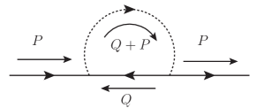
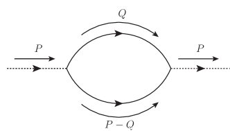
Figure 1: The one-loop (a) fermion and (b) boson self-energy diagrams.

Let us now compute one-loop self-energy corrections. A sample contraction of terms leading to the fermion self-energy can be written as:

ϕ(ψTΓ45ψ)ϕ(ψΓ45ψ)=(ϕϕ)ψα(Γ45)α,βψβψγ(Γ45)γ,δψδ=ψδ[(Γ45)δ,γ(G0T)γ,β(Γ45)β,αD0]ψα.superscriptitalic-ϕsuperscript𝜓𝑇subscriptΓ45𝜓italic-ϕsuperscript𝜓subscriptΓ45superscript𝜓superscriptitalic-ϕitalic-ϕsubscript𝜓𝛼superscriptsubscriptΓ45𝛼𝛽subscript𝜓𝛽subscriptsuperscript𝜓𝛾superscriptsubscriptΓ45𝛾𝛿subscriptsuperscript𝜓𝛿subscriptsuperscript𝜓𝛿delimited-[]superscriptsubscriptΓ45𝛿𝛾subscriptsuperscriptsubscript𝐺0𝑇𝛾𝛽superscriptsubscriptΓ45𝛽𝛼subscript𝐷0subscript𝜓𝛼\displaystyle\phi^{*}\left(\psi^{T}\,\Gamma_{45}\,\psi\right)\phi\left(\psi^{\dagger}\,\Gamma_{45}\,\psi^{*}\right)=\left(\phi^{*}\phi\right)\psi_{\alpha}\,\left(\Gamma_{45}\right)^{\alpha,\beta}\,\psi_{\beta}\,\psi^{*}_{\gamma}\,\left(\Gamma_{45}\right)^{\gamma,\delta}\,\psi^{*}_{\delta}=-\psi^{*}_{\delta}\left[\left(\Gamma_{45}\right)^{\delta,\gamma}\left(G_{0}^{T}\right)_{\gamma,\beta}\left(\Gamma_{45}\right)^{\beta,\alpha}\,D_{0}\right]\psi_{\alpha}\,.

There are two such terms possible. Similarly, a sample contraction of terms leading to the boson self-energy can be written as:

ϕ(ψTΓ45ψ)ϕ(ψΓ45ψ)=ϕϕ[ψα(Γ45)α,βψβ][ψγ(Γ45)γ,δψδ]superscriptitalic-ϕsuperscript𝜓𝑇subscriptΓ45𝜓italic-ϕsuperscript𝜓subscriptΓ45superscript𝜓italic-ϕsuperscriptitalic-ϕdelimited-[]subscript𝜓𝛼superscriptsubscriptΓ45𝛼𝛽subscript𝜓𝛽delimited-[]subscriptsuperscript𝜓𝛾superscriptsubscriptΓ45𝛾𝛿subscriptsuperscript𝜓𝛿\displaystyle\phi^{*}\left(\psi^{T}\,\Gamma_{45}\,\psi\right)\phi\left(\psi^{\dagger}\,\Gamma_{45}\,\psi^{*}\right)=\phi\,\phi^{*}\left[\psi_{\alpha}\left(\Gamma_{45}\right)^{\alpha,\beta}\psi_{\beta}\right]\left[\psi^{*}_{\gamma}\left(\Gamma_{45}\right)^{\gamma,\delta}\,\psi^{*}_{\delta}\right]
=ϕϕ[(G0T)δ,α(Γ45)α,β(G0)β,γ(Γ45)γ,δ]=ϕϕTr[G0TΓ45G0Γ45].absentitalic-ϕsuperscriptitalic-ϕdelimited-[]subscriptsuperscriptsubscript𝐺0𝑇𝛿𝛼superscriptsubscriptΓ45𝛼𝛽subscriptsubscript𝐺0𝛽𝛾superscriptsubscriptΓ45𝛾𝛿italic-ϕsuperscriptitalic-ϕTrdelimited-[]superscriptsubscript𝐺0𝑇subscriptΓ45subscript𝐺0subscriptΓ45\displaystyle=\phi\,\phi^{*}\left[\left(G_{0}^{T}\right)_{\delta,\alpha}\left(\Gamma_{45}\right)^{\alpha,\beta}\left(G_{0}\right)_{\beta,\gamma}\left(\Gamma_{45}\right)^{\gamma,\delta}\right]=\phi\,\phi^{*}{\rm Tr}\,\left[G_{0}^{T}\,\Gamma_{45}\,G_{0}\,\Gamma_{45}\right].

Again, there can be two such terms.

The explicit expressions for the fermion and self-energies are given by:

Σ1(P)subscriptΣ1𝑃\displaystyle\Sigma_{1}(P) =g2μεQD0(Q+P)Γ45G0T(Q)Γ45, andabsentsuperscript𝑔2superscript𝜇𝜀subscript𝑄subscript𝐷0𝑄𝑃subscriptΓ45superscriptsubscript𝐺0T𝑄subscriptΓ45 and\displaystyle=-g^{2}\mu^{\varepsilon}\int_{Q}D_{0}(Q+P)\,\Gamma_{45}\,G_{0}^{\rm T}(Q)\,\Gamma_{45}\,,\text{ and } (8)
Π1(P)subscriptΠ1𝑃\displaystyle\Pi_{1}(P) =g2μεQTr[Γ45G0(Q)Γ45G0T(PQ)],absentsuperscript𝑔2superscript𝜇𝜀subscript𝑄Trdelimited-[]subscriptΓ45subscript𝐺0𝑄subscriptΓ45superscriptsubscript𝐺0T𝑃𝑄\displaystyle=g^{2}\mu^{\varepsilon}\int_{Q}{\rm Tr}\,\left[\Gamma_{45}\,G_{0}(Q)\,\Gamma_{45}\,G_{0}^{\rm T}(P-Q)\right], (9)

respectively, as can be seen in Fig. 1. Throughout the paper, we have denoted the integrals by:

Q=q0𝐪,q0=dq02π,𝐪=ddq(2π)d.formulae-sequencesubscript𝑄subscriptsubscript𝑞0subscript𝐪formulae-sequencesubscriptsubscript𝑞0dsubscript𝑞02𝜋subscript𝐪superscriptd𝑑𝑞superscript2𝜋𝑑\displaystyle\int_{Q}=\int_{q_{0}}\int_{{\bf q}}\,,\quad\int_{q_{0}}=\int\frac{\mbox{d}q_{0}}{2\pi}\,,\quad\int_{{\bf q}}=\int\frac{\mbox{d}^{d}q}{(2\pi)^{d}}\,. (10)

Using Eq. (107), we get:

Σ1(P)subscriptΣ1𝑃\displaystyle\Sigma_{1}(P) =g2μεQD0(Q+P)G0(Q)absentsuperscript𝑔2superscript𝜇𝜀subscript𝑄subscript𝐷0𝑄𝑃subscript𝐺0𝑄\displaystyle=-g^{2}\mu^{\varepsilon}\int_{Q}D_{0}(Q+P)\,G_{0}(Q)
=g2μεQ(iq0+ξq2)𝟙N𝐝(𝐪)𝚪[q02+(1ξ2)q42iq0ξq2][iy(q0+p0)+(𝐪+𝐩)2],absentsuperscript𝑔2superscript𝜇𝜀subscript𝑄𝑖subscript𝑞0𝜉superscript𝑞2subscriptdouble-struck-𝟙𝑁𝐝𝐪𝚪delimited-[]superscriptsubscript𝑞021superscript𝜉2superscript𝑞42𝑖subscript𝑞0𝜉superscript𝑞2delimited-[]𝑖𝑦subscript𝑞0subscript𝑝0superscript𝐪𝐩2\displaystyle=g^{2}\mu^{\varepsilon}\int_{Q}\frac{\left(i\,q_{0}+\xi\,q^{2}\right)\mathbb{1}_{N}-{\bf d}({\bf q})\cdot{\bf\Gamma}}{\left[\,q_{0}^{2}+\left(1-\xi^{2}\right)q^{4}-2\,i\,q_{0}\,\xi\,q^{2}\right]\left[i\,y\,\left(q_{0}+p_{0}\right)+\left(\mathbf{q}+\mathbf{p}\right)^{2}\right]}\,, (11)
Π1(P)subscriptΠ1𝑃\displaystyle\Pi_{1}(P) =g2μεQTr[G0(Q)G0(PQ)].absentsuperscript𝑔2superscript𝜇𝜀subscript𝑄Trdelimited-[]subscript𝐺0𝑄subscript𝐺0𝑃𝑄\displaystyle=g^{2}\mu^{\varepsilon}\int_{Q}{\rm Tr}\,\left[G_{0}(Q)\,G_{0}(P-Q)\right]. (12)

Performing the trace in the numerator of Π1subscriptΠ1\Pi_{1} yields

Tr[{iq0+ξq2𝐝(𝐪)𝚪}{i(p0q0)+ξ(𝐩𝐪)2𝐝(𝐩𝐪)𝚪}]Trdelimited-[]𝑖subscript𝑞0𝜉superscript𝑞2𝐝𝐪𝚪𝑖subscript𝑝0subscript𝑞0𝜉superscript𝐩𝐪2𝐝𝐩𝐪𝚪\displaystyle{\rm Tr}\,\left[\left\{i\,q_{0}+\xi\,q^{2}-{\bf d}({\bf q})\cdot{\bf\Gamma}\right\}\left\{i\,\left(p_{0}-q_{0}\right)+\xi\,\left({\bf p}-{\bf q}\right)^{2}-{\bf d}\left({\bf p}-{\bf q}\right)\cdot{\bf\Gamma}\right\}\right]
=N[(iq0ξq2){i(q0p0)ξ(𝐪𝐩)2}+da(𝐪)da(𝐪𝐩)]absent𝑁delimited-[]𝑖subscript𝑞0𝜉superscript𝑞2𝑖subscript𝑞0subscript𝑝0𝜉superscript𝐪𝐩2subscript𝑑𝑎𝐪subscript𝑑𝑎𝐪𝐩\displaystyle=N\Bigl{[}(-i\,q_{0}-\xi\,q^{2})\Big{\{}i\left(q_{0}-p_{0}\right)-\xi\left({\bf q}-{\bf p}\right)^{2}\Big{\}}+d_{a}({\bf q})\,d_{a}({\bf q}-{\bf p})\Bigr{]}
=N[(iq0ξq2){i(q0p0)ξ(𝐪𝐩)2}+43{𝐪(𝐪𝐩)}2q23(𝐪𝐩)2],absent𝑁delimited-[]𝑖subscript𝑞0𝜉superscript𝑞2𝑖subscript𝑞0subscript𝑝0𝜉superscript𝐪𝐩243superscript𝐪𝐪𝐩2superscript𝑞23superscript𝐪𝐩2\displaystyle=N\Bigl{[}(-i\,q_{0}-\xi\,q^{2})\Big{\{}i\left(q_{0}-p_{0}\right)-\xi\left({\bf q}-{\bf p}\right)^{2}\Big{\}}+\frac{4}{3}\big{\{}{\bf q}\cdot({\bf q}-{\bf p})\big{\}}^{2}-\frac{q^{2}}{3}({\bf q}-{\bf p})^{2}\Bigr{]}\,, (13)

where we have used Eq. (118). Therefore,

Π1(P)=Qg2μεN[(iq0ξq2){i(q0p0)ξ(𝐪𝐩)2}+43{𝐪(𝐪𝐩)}2q23(𝐪𝐩)2][q02+(1ξ2)q42iq0ξq2][(p0q0)2+(1ξ2)(𝐩𝐪)42i(p0q0)ξ(𝐩𝐪)2].subscriptΠ1𝑃subscript𝑄superscript𝑔2superscript𝜇𝜀𝑁delimited-[]𝑖subscript𝑞0𝜉superscript𝑞2𝑖subscript𝑞0subscript𝑝0𝜉superscript𝐪𝐩243superscript𝐪𝐪𝐩2superscript𝑞23superscript𝐪𝐩2delimited-[]superscriptsubscript𝑞021superscript𝜉2superscript𝑞42𝑖subscript𝑞0𝜉superscript𝑞2delimited-[]superscriptsubscript𝑝0subscript𝑞021superscript𝜉2superscript𝐩𝐪42𝑖subscript𝑝0subscript𝑞0𝜉superscript𝐩𝐪2\displaystyle\Pi_{1}(P)=\int_{Q}\frac{g^{2}\mu^{\varepsilon}\,N\Bigl{[}(-i\,q_{0}-\xi\,q^{2})\Big{\{}i\left(q_{0}-p_{0}\right)-\xi\left({\bf q}-{\bf p}\right)^{2}\Big{\}}+\frac{4}{3}\big{\{}{\bf q}\cdot({\bf q}-{\bf p})\big{\}}^{2}-\frac{q^{2}}{3}({\bf q}-{\bf p})^{2}\Bigr{]}}{\left[q_{0}^{2}+\left(1-\xi^{2}\right)q^{4}-2\,i\,q_{0}\,\xi\,q^{2}\right]\,\left[\left(p_{0}-q_{0}\right)^{2}+\left(1-\xi^{2}\right)\left({\bf p}-{\bf q}\right)^{4}-2\,i\left(p_{0}-q_{0}\right)\xi\left({\bf p}-{\bf q}\right)^{2}\right]}\,. (14)

For the fermion self-energy, we first integrate over q0subscript𝑞0q_{0}, and then complete the squares in the denominator (using Feynman parametrization, if necessary) to make it easy to perform the 𝐪𝐪\mathbf{q}-integral:

Σ1(P)subscriptΣ1𝑃\displaystyle\Sigma_{1}(P) =g2με2𝐪1𝐝(𝐪)𝚪q2ip0y+q2(1+yξy)+p2+2𝐩𝐪absentsuperscript𝑔2superscript𝜇𝜀2subscript𝐪1𝐝𝐪𝚪superscript𝑞2𝑖subscript𝑝0𝑦superscript𝑞21𝑦𝜉𝑦superscript𝑝22𝐩𝐪\displaystyle=\frac{g^{2}\mu^{\varepsilon}}{2}\int_{{\bf q}}\frac{1-\frac{\mathbf{d}(\mathbf{q})\cdot\mathbf{\Gamma}}{q^{2}}}{i\,p_{0}\,y+q^{2}\left(1+y-\xi\,y\right)+p^{2}+2\,\mathbf{p}\cdot\mathbf{q}}
=p2g2y(1ξ)(μp)ε16π2(y+1ξy)3εip0g2y(μ|p0|)ε16π2(y+1ξy)2ε+[𝐝(𝐩)𝚪]g2(μp)ε48π2(y+1ξy)3ε+𝒪(ε0),absentsuperscript𝑝2superscript𝑔2𝑦1𝜉superscript𝜇𝑝𝜀16superscript𝜋2superscript𝑦1𝜉𝑦3𝜀𝑖subscript𝑝0superscript𝑔2𝑦superscript𝜇subscript𝑝0𝜀16superscript𝜋2superscript𝑦1𝜉𝑦2𝜀delimited-[]𝐝𝐩𝚪superscript𝑔2superscript𝜇𝑝𝜀48superscript𝜋2superscript𝑦1𝜉𝑦3𝜀𝒪superscript𝜀0\displaystyle=-\frac{p^{2}\,g^{2}\,y\left(1-\xi\right)\left(\frac{\mu}{p}\right)^{\varepsilon}}{16\,\pi^{2}\left(y+1-\xi\,y\right)^{3}\varepsilon}-\frac{i\,p_{0}\,g^{2}\,y\,\left(\frac{\mu}{\sqrt{\left|p_{0}\right|}}\right)^{\varepsilon}}{16\,\pi^{2}\left(y+1-\xi\,y\right)^{2}\varepsilon}+\frac{\left[\mathbf{d}(\mathbf{p})\cdot\mathbf{\Gamma}\right]g^{2}\left(\frac{\mu}{p}\right)^{\varepsilon}}{48\,\pi^{2}\left(y+1-\xi\,y\right)^{3}\varepsilon}+\mathcal{O}\left(\varepsilon^{0}\right), (15)

where, in the second line, we have used the relation in Eqs. (118) and (121).

For the boson self-energy, we integrate over q0subscript𝑞0q_{0}, employ partial fraction decomposition, complete the squares in the denominator (using Feynman parametrization, if necessary), before finally integrating over 𝐪𝐪\mathbf{q}:

Π1(P)subscriptΠ1𝑃\displaystyle\Pi_{1}(P) =13ip0g2Nξ(μ|p0|)ε288π2(1ξ2)2ε107p2g2N(μp)ε3456π2(1ξ2)ε+𝒪(ε0).absent13𝑖subscript𝑝0superscript𝑔2𝑁𝜉superscript𝜇subscript𝑝0𝜀288superscript𝜋2superscript1superscript𝜉22𝜀107superscript𝑝2superscript𝑔2𝑁superscript𝜇𝑝𝜀3456superscript𝜋21superscript𝜉2𝜀𝒪superscript𝜀0\displaystyle=\frac{13\,i\,p_{0}\,g^{2}\,N\,\xi\left(\frac{\mu}{\sqrt{\left|p_{0}\right|}}\right)^{\varepsilon}}{288\,\pi^{2}\left(1-\xi^{2}\right)^{2}\varepsilon}-\frac{107\,p^{2}\,g^{2}\,N\left(\frac{\mu}{p}\right)^{\varepsilon}}{3456\,\pi^{2}\left(1-\xi^{2}\right)\varepsilon}+\mathcal{O}\left(\varepsilon^{0}\right). (16)

III.2 RG equations

The counterterm action is given by:

𝒮CT=subscript𝒮𝐶𝑇absent\displaystyle{\mathcal{S}}_{CT}= P[ψ(P){A1ip0+A2da(𝐩)Γa+A3ξp2}ψ(P)+ϕ(P)(A4iyp0+A5p2)ϕ(P)]subscript𝑃delimited-[]superscript𝜓𝑃subscript𝐴1𝑖subscript𝑝0subscript𝐴2subscript𝑑𝑎𝐩subscriptΓ𝑎subscript𝐴3𝜉superscript𝑝2𝜓𝑃superscriptitalic-ϕ𝑃subscript𝐴4𝑖𝑦subscript𝑝0subscript𝐴5superscript𝑝2italic-ϕ𝑃\displaystyle\int_{P}\Big{[}{\psi}^{\dagger}(P)\left\{A_{1}\,i\,p_{0}+A_{2}\,d_{a}\left({\bf p}\right)\,\Gamma_{a}+A_{3}\,{\xi}\,p^{2}\right\}{\psi}(P)+{\phi}^{*}(P)\left(A_{4}\,i\,{y}\,p_{0}+A_{5}\,p^{2}\right){\phi}(P)\Big{]}
+gμε/2PKA6[ϕ(P)ψ(K)Γ45ψ(PK)+ϕ(P)ψT(PK)Γ45ψ(K)],𝑔superscript𝜇𝜀2subscript𝑃subscript𝐾subscript𝐴6delimited-[]italic-ϕ𝑃superscript𝜓𝐾subscriptΓ45superscript𝜓𝑃𝐾superscriptitalic-ϕ𝑃superscript𝜓T𝑃𝐾subscriptΓ45𝜓𝐾\displaystyle+{g}\,\mu^{\varepsilon/2}\int_{P}\int_{K}A_{6}\left[{\phi}(P)\,{\psi}^{\dagger}(K)\,\Gamma_{45}\,{\psi}^{*}(P-K)+{\phi}^{*}(P)\,{\psi}^{\rm T}(P-K)\,\Gamma_{45}\,{\psi}(K)\right],
Ansubscript𝐴𝑛\displaystyle A_{n} Zn1=λ=1Zn,λελ with n=1,2,3,4,5,6.formulae-sequenceabsentsubscript𝑍𝑛1superscriptsubscript𝜆1subscript𝑍𝑛𝜆superscript𝜀𝜆 with 𝑛123456\displaystyle\equiv\,Z_{n}-1=\sum_{\lambda=1}^{\infty}\frac{Z_{n,\lambda}}{\varepsilon^{\lambda}}\text{ with }n=1,2,3,4,5,6\,. (17)

Adding the counterterms to the original 𝒮0subscript𝒮0\mathcal{S}_{0}, and denoting the bare quantities by the index “B”, we obtain the renormalized action as:

𝒮rensubscript𝒮𝑟𝑒𝑛\displaystyle{\mathcal{S}}_{ren} =PB[ψ(PB){ip0B+da(𝐩B)Γa+ξBpB2}ψ(PB)+ϕ(PB)(iyBp0B+pB2)ϕ(PB)]absentsubscriptsubscript𝑃𝐵delimited-[]superscript𝜓subscript𝑃𝐵𝑖subscript𝑝subscript0𝐵subscript𝑑𝑎subscript𝐩𝐵subscriptΓ𝑎subscript𝜉𝐵superscriptsubscript𝑝𝐵2𝜓subscript𝑃𝐵superscriptitalic-ϕsubscript𝑃𝐵𝑖subscript𝑦𝐵subscript𝑝subscript0𝐵superscriptsubscript𝑝𝐵2italic-ϕsubscript𝑃𝐵\displaystyle=\int_{P_{B}}\Big{[}{\psi}^{\dagger}(P_{B})\left\{i\,p_{0_{B}}+d_{a}\left({\bf p}_{B}\right)\,\Gamma_{a}+{\xi}_{B}\,p_{B}^{2}\right\}{\psi}(P_{B})+{\phi}^{*}(P_{B})\left(i\,{y}_{B}\,p_{0_{B}}+p_{B}^{2}\right){\phi}(P_{B})\Big{]}
+gBPBKB[ϕ(PB)ψ(KB)Γ45ψ(PBKB)+ϕ(PB)ψT(PBKB)Γ45ψ(KB)].subscript𝑔𝐵subscriptsubscript𝑃𝐵subscriptsubscript𝐾𝐵delimited-[]italic-ϕsubscript𝑃𝐵superscript𝜓subscript𝐾𝐵subscriptΓ45superscript𝜓subscript𝑃𝐵subscript𝐾𝐵superscriptitalic-ϕsubscript𝑃𝐵superscript𝜓Tsubscript𝑃𝐵subscript𝐾𝐵subscriptΓ45𝜓subscript𝐾𝐵\displaystyle+{g}_{B}\int_{P_{B}}\int_{K_{B}}\left[{\phi}(P_{B})\,{\psi}^{\dagger}(K_{B})\,\Gamma_{45}\,{\psi}^{*}(P_{B}-K_{B})+{\phi}^{*}(P_{B})\,{\psi}^{\rm T}(P_{B}-K_{B})\,\Gamma_{45}\,{\psi}(K_{B})\right]. (18)

The bare and renormalized quantitites are related by the following convention:

(p0)B=Z1p0,𝐩B=Z2𝐩,ψB(PB)=Zψψ(P),ϕB(PB)=Zϕϕ(P),formulae-sequencesubscriptsubscript𝑝0𝐵subscript𝑍1subscript𝑝0formulae-sequencesubscript𝐩𝐵subscript𝑍2𝐩formulae-sequencesubscript𝜓𝐵subscript𝑃𝐵subscript𝑍𝜓𝜓𝑃subscriptitalic-ϕ𝐵subscript𝑃𝐵subscript𝑍italic-ϕitalic-ϕ𝑃\displaystyle(p_{0})_{B}=Z_{1}\,p_{0}\,,\quad{\bf p}_{B}=\sqrt{Z_{2}}\,{\bf p}\,,\quad\psi_{B}(P_{B})=\sqrt{Z_{\psi}}\,\psi(P)\,,\quad\phi_{B}(P_{B})=\sqrt{Z_{\phi}}\,\phi(P)\,,
ξB=Z3Z2ξ,yB=Z2Z4Z1Z5y,gB=Z6Z21d+24Z1Z5gμε/2,Zψ=1Z1Z2d2,Zϕ=Z5Z1Z21+d2,formulae-sequencesubscript𝜉𝐵subscript𝑍3subscript𝑍2𝜉formulae-sequencesubscript𝑦𝐵subscript𝑍2subscript𝑍4subscript𝑍1subscript𝑍5𝑦formulae-sequencesubscript𝑔𝐵subscript𝑍6superscriptsubscript𝑍21𝑑24subscript𝑍1subscript𝑍5𝑔superscript𝜇𝜀2formulae-sequencesubscript𝑍𝜓1subscript𝑍1superscriptsubscript𝑍2𝑑2subscript𝑍italic-ϕsubscript𝑍5subscript𝑍1superscriptsubscript𝑍21𝑑2\displaystyle\xi_{B}=\frac{Z_{3}}{Z_{2}}\,\xi\,,\quad y_{B}=\frac{Z_{2}\,Z_{4}}{Z_{1}\,Z_{5}}\,y\,,\quad g_{B}=\frac{Z_{6}\,Z_{2}^{1-\frac{d+2}{4}}}{\sqrt{Z_{1}\,Z_{5}}}\,g\,\mu^{\varepsilon/2},\quad Z_{\psi}=\frac{1}{Z_{1}\,Z_{2}^{\frac{d}{2}}}\,,\quad Z_{\phi}=\frac{Z_{5}}{Z_{1}\,Z_{2}^{1+\frac{d}{2}}}\,, (19)

with the tree-level mass dimensions [p0]=2delimited-[]subscript𝑝02[p_{0}]=2, [𝐩]=1delimited-[]𝐩1[{\bf p}]=1, [ξ]=[y]=0.delimited-[]𝜉delimited-[]𝑦0[\xi]=[y]=0\,.

Let us define:

zτ=2+lnZ1lnμ,zr=1+12lnZ1lnμ,ηψ=12lnZψlnμ,ηϕ=12lnZϕlnμ,formulae-sequencesubscript𝑧𝜏2subscript𝑍1𝜇formulae-sequencesubscript𝑧𝑟112subscript𝑍1𝜇formulae-sequencesubscript𝜂𝜓12subscript𝑍𝜓𝜇subscript𝜂italic-ϕ12subscript𝑍italic-ϕ𝜇\displaystyle z_{\tau}=2+\frac{\partial\ln{Z_{1}}}{\partial\ln\mu}\,,\quad z_{r}=1+\frac{1}{2}\frac{\partial\ln{Z_{1}}}{\partial\ln\mu}\,,\quad\eta_{\psi}=\frac{1}{2}\frac{\partial\ln Z_{\psi}}{\partial\ln\mu}\,,\quad\eta_{\phi}=\frac{1}{2}\frac{\partial\ln Z_{\phi}}{\partial\ln\mu}\,, (20)

where zτsubscript𝑧𝜏z_{\tau} and zrsubscript𝑧𝑟z_{r} are the quantum scaling dimensions for k0subscript𝑘0k_{0} and 𝐤𝐤\mathbf{k}, respectively. Furthermore, ηψsubscript𝜂𝜓\eta_{\psi} and ηϕsubscript𝜂italic-ϕ\eta_{\phi} are the anomalous dimensions of the fermion and the boson, respectively, and can be expressed as:

2ηψ2subscript𝜂𝜓\displaystyle 2\,\eta_{\psi} =2+dzτdzr,2ηϕ=4+dzτ(2+d)zr+1Z5Z5lnμ.formulae-sequenceabsent2𝑑subscript𝑧𝜏𝑑subscript𝑧𝑟2subscript𝜂italic-ϕ4𝑑subscript𝑧𝜏2𝑑subscript𝑧𝑟1subscript𝑍5subscript𝑍5𝜇\displaystyle={2+d-z_{\tau}-d\,z_{r}}\,,\quad 2\,\eta_{\phi}=4+d-z_{\tau}-\left(2+d\right)z_{r}+\frac{1}{Z_{5}}\frac{\partial Z_{5}}{\partial\ln\mu}\,. (21)

Since the bare quantitites do not depend on μ𝜇\mu, their total derivative with respect to μ𝜇\mu should vanish. Therefore, dlngBdlnμ=0𝑑subscript𝑔𝐵𝑑𝜇0\frac{d\ln g_{B}}{d\ln\mu}=0 gives:

glnμβg=[ε2+(1d2)(zr1)12lnZ5lnμ+lnZ6lnμ+1zτ2]g.𝑔𝜇subscript𝛽𝑔delimited-[]𝜀21𝑑2subscript𝑧𝑟112subscript𝑍5𝜇subscript𝑍6𝜇1subscript𝑧𝜏2𝑔\displaystyle-\frac{\partial g}{\partial\ln\mu}\equiv-\beta_{g}=\left[\frac{\varepsilon}{2}+\left(1-\frac{d}{2}\right)\left(z_{r}-1\right)-\frac{1}{2}\frac{\partial\ln Z_{5}}{\partial\ln\mu}+\frac{\partial\ln Z_{6}}{\partial\ln\mu}+1-\frac{z_{\tau}}{2}\right]\,g\,. (22)

To one-loop order, we have Zn=1+Zn,1εsubscript𝑍𝑛1subscript𝑍𝑛1𝜀Z_{n}=1+\frac{Z_{n,1}}{\varepsilon}, where

Z1,1subscript𝑍11\displaystyle Z_{1,1} =g2y16π2(1+yξy)2,Z2,1=g248π2(1+yξy)3,Z3,1=g2y(1ξ)16π2(1+yξy)3ξ,formulae-sequenceabsentsuperscript𝑔2𝑦16superscript𝜋2superscript1𝑦𝜉𝑦2formulae-sequencesubscript𝑍21superscript𝑔248superscript𝜋2superscript1𝑦𝜉𝑦3subscript𝑍31superscript𝑔2𝑦1𝜉16superscript𝜋2superscript1𝑦𝜉𝑦3𝜉\displaystyle=-\frac{g^{2}\,y}{16\,\pi^{2}\left(1+y-\xi\,y\right)^{2}}\,,\quad Z_{2,1}=\frac{g^{2}}{48\,\pi^{2}\left(1+y-\xi\,y\right)^{3}}\,,\quad Z_{3,1}=-\frac{g^{2}\,y\left(1-\xi\right)}{16\,\pi^{2}\left(1+y-\xi\,y\right)^{3}\xi}\,,
Z4,1subscript𝑍41\displaystyle Z_{4,1} =13Ng2ξ288π2(1ξ2)2y,Z5,1=107Ng23456π2(1ξ2),Z6,1=0.formulae-sequenceabsent13𝑁superscript𝑔2𝜉288superscript𝜋2superscript1superscript𝜉22𝑦formulae-sequencesubscript𝑍51107𝑁superscript𝑔23456superscript𝜋21superscript𝜉2subscript𝑍610\displaystyle=\frac{13\,N\,g^{2}\,\xi}{288\,\pi^{2}\left(1-\xi^{2}\right)^{2}y}\,,\quad Z_{5,1}=-\frac{107\,N\,g^{2}}{3456\,\pi^{2}\left(1-\xi^{2}\right)}\,,\quad Z_{6,1}=0\,. (23)

Using the expansions:

zτ=zτ(0),zr=zr(0),ηψ=ηψ(0)+εηψ(1),ηϕ=ηϕ(0)+εηϕ(1),formulae-sequencesubscript𝑧𝜏subscriptsuperscript𝑧0𝜏formulae-sequencesubscript𝑧𝑟subscriptsuperscript𝑧0𝑟formulae-sequencesubscript𝜂𝜓superscriptsubscript𝜂𝜓0𝜀superscriptsubscript𝜂𝜓1subscript𝜂italic-ϕsuperscriptsubscript𝜂italic-ϕ0𝜀superscriptsubscript𝜂italic-ϕ1\displaystyle z_{\tau}=z^{(0)}_{\tau}\,,\quad z_{r}=z^{(0)}_{r}\,,\quad\eta_{\psi}=\eta_{\psi}^{(0)}+\varepsilon\,\eta_{\psi}^{(1)}\,,\quad\eta_{\phi}=\eta_{\phi}^{(0)}+\varepsilon\,\eta_{\phi}^{(1)}\,,
βξ=βξ(0)+εβξ(1),βy=βy(0)+εβy(1),βg=βg(0)+εβg(1),formulae-sequencesubscript𝛽𝜉superscriptsubscript𝛽𝜉0𝜀superscriptsubscript𝛽𝜉1formulae-sequencesubscript𝛽𝑦superscriptsubscript𝛽𝑦0𝜀superscriptsubscript𝛽𝑦1subscript𝛽𝑔superscriptsubscript𝛽𝑔0𝜀superscriptsubscript𝛽𝑔1\displaystyle\beta_{\xi}=\beta_{\xi}^{(0)}+\varepsilon\,\beta_{\xi}^{(1)}\,,\quad\beta_{y}=\beta_{y}^{(0)}+\varepsilon\,\beta_{y}^{(1)}\,,\quad\beta_{g}=\beta_{g}^{(0)}+\varepsilon\,\beta_{g}^{(1)}\,, (24)

and comparing the powers of ε𝜀\varepsilon from the μ𝜇\mu-derivatives of the Eqs. (III.2), we get:

zτ=2+g2y16π2(1+yξy)2,zr=1g296π2(1+yξy)3,formulae-sequencesubscript𝑧𝜏2superscript𝑔2𝑦16superscript𝜋2superscript1𝑦𝜉𝑦2subscript𝑧𝑟1superscript𝑔296superscript𝜋2superscript1𝑦𝜉𝑦3\displaystyle z_{\tau}=2+\frac{g^{2}\,y}{16\,\pi^{2}\left(1+y-\xi\,y\right)^{2}}\,,\quad z_{r}=1-\frac{g^{2}}{96\,\pi^{2}\left(1+y-\xi\,y\right)^{3}}\,,
ηψ=g2ε192π2(1+yξy)3+g248π2(1+yξy)3g2y32π2(1+yξy)2,subscript𝜂𝜓superscript𝑔2𝜀192superscript𝜋2superscript1𝑦𝜉𝑦3superscript𝑔248superscript𝜋2superscript1𝑦𝜉𝑦3superscript𝑔2𝑦32superscript𝜋2superscript1𝑦𝜉𝑦2\displaystyle\eta_{\psi}=-\frac{g^{2}\,\varepsilon}{192\,\pi^{2}\left(1+y-\xi\,y\right)^{3}}+\frac{g^{2}}{48\,\pi^{2}\left(1+y-\xi\,y\right)^{3}}-\frac{g^{2}\,y}{32\,\pi^{2}\left(1+y-\xi\,y\right)^{2}}\,,
ηϕ=g2ε192π2(1+yξy)3+g2π2[107N6912(1ξ2)y32(1+yξy)2+132(1+yξy)3],subscript𝜂italic-ϕsuperscript𝑔2𝜀192superscript𝜋2superscript1𝑦𝜉𝑦3superscript𝑔2superscript𝜋2delimited-[]107𝑁69121superscript𝜉2𝑦32superscript1𝑦𝜉𝑦2132superscript1𝑦𝜉𝑦3\displaystyle\eta_{\phi}=-\frac{g^{2}\,\varepsilon}{192\,\pi^{2}\left(1+y-\xi\,y\right)^{3}}+\frac{g^{2}}{\pi^{2}}\left[\frac{107\,N}{6912\left(1-\xi^{2}\right)}-\frac{y}{32\left(1+y-\xi\,y\right)^{2}}+\frac{1}{32\left(1+y-\xi\,y\right)^{3}}\right]\,, (25)

and the beta-functions:

βξ=ξ+3(1ξ)y48π2(1+yξy)3g2,subscript𝛽𝜉𝜉31𝜉𝑦48superscript𝜋2superscript1𝑦𝜉𝑦3superscript𝑔2\displaystyle\beta_{\xi}=-\frac{\xi+3\left(1-\xi\right)y}{48\,\pi^{2}\left(1+y-\xi\,y\right)^{3}}\,g^{2}\,,
βy=g2π2[13Nξ288(1ξ2)2+107Ny3456(1ξ2)+y216(1+yξy)2+y48(1+yξy)3],subscript𝛽𝑦superscript𝑔2superscript𝜋2delimited-[]13𝑁𝜉288superscript1superscript𝜉22107𝑁𝑦34561superscript𝜉2superscript𝑦216superscript1𝑦𝜉𝑦2𝑦48superscript1𝑦𝜉𝑦3\displaystyle\beta_{y}=\frac{g^{2}}{\pi^{2}}\left[\frac{13\,N\,\xi}{288\left(1-\xi^{2}\right)^{2}}+\frac{107\,N\,y}{3456\left(1-\xi^{2}\right)}+\frac{y^{2}}{16\left(1+y-\xi\,y\right)^{2}}+\frac{y}{48\left(1+y-\xi\,y\right)^{3}}\right]\,,
βg=εg2+g3π2[107N6912(1ξ2)+y32(1+yξy)2196(1+yξy)3].subscript𝛽𝑔𝜀𝑔2superscript𝑔3superscript𝜋2delimited-[]107𝑁69121superscript𝜉2𝑦32superscript1𝑦𝜉𝑦2196superscript1𝑦𝜉𝑦3\displaystyle\beta_{g}=-\frac{\varepsilon\,g}{2}+\frac{g^{3}}{\pi^{2}}\left[\frac{107\,N}{6912\left(1-\xi^{2}\right)}+\frac{y}{32\left(1+y-\xi\,y\right)^{2}}-\frac{1}{96\left(1+y-\xi\,y\right)^{3}}\right]. (26)

III.3 Fixed points and their stability

The fixed points (ξ,y,g)superscript𝜉superscript𝑦superscript𝑔\left(\xi^{*},y^{*},{g}^{*}\right) are given by:

(0, 0, 0) and (0, 0,±246πε107N72).0 0 0 and 0 0plus-or-minus246𝜋𝜀107𝑁72\displaystyle\left(0,\,0,\,0\right)\text{ and }\left(0,\,0,\,\pm\frac{24\,\sqrt{6}\,\pi\,\sqrt{\varepsilon}}{\sqrt{107\,N-72}}\right). (27)
Refer to caption
Refer to caption
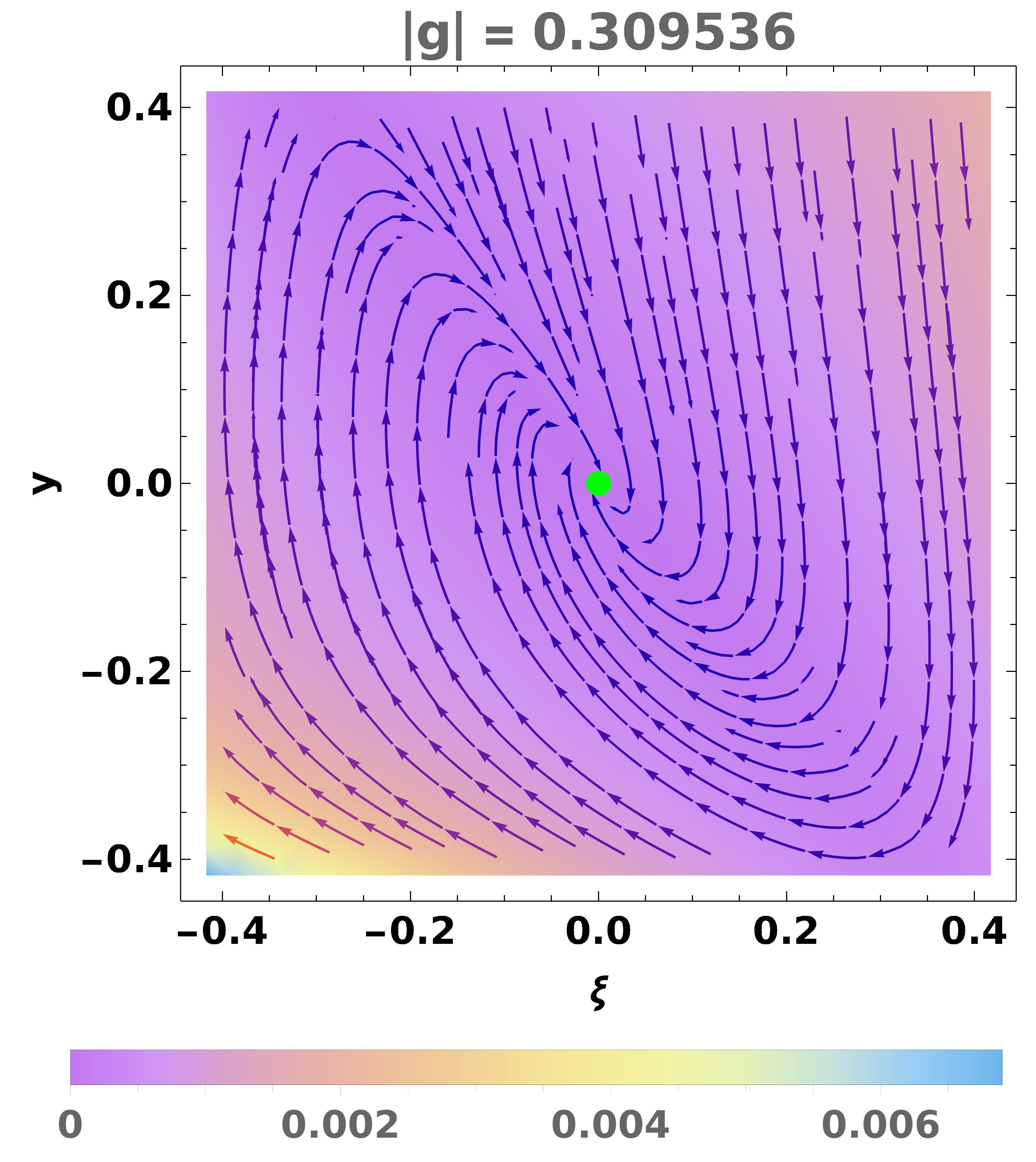
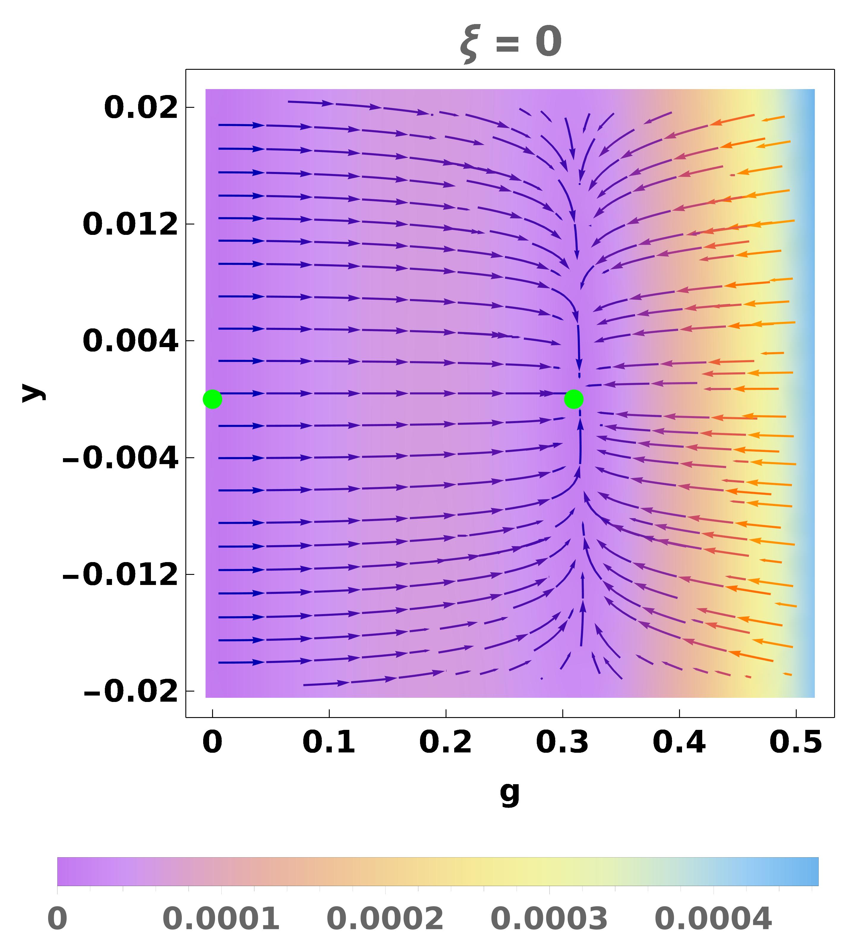
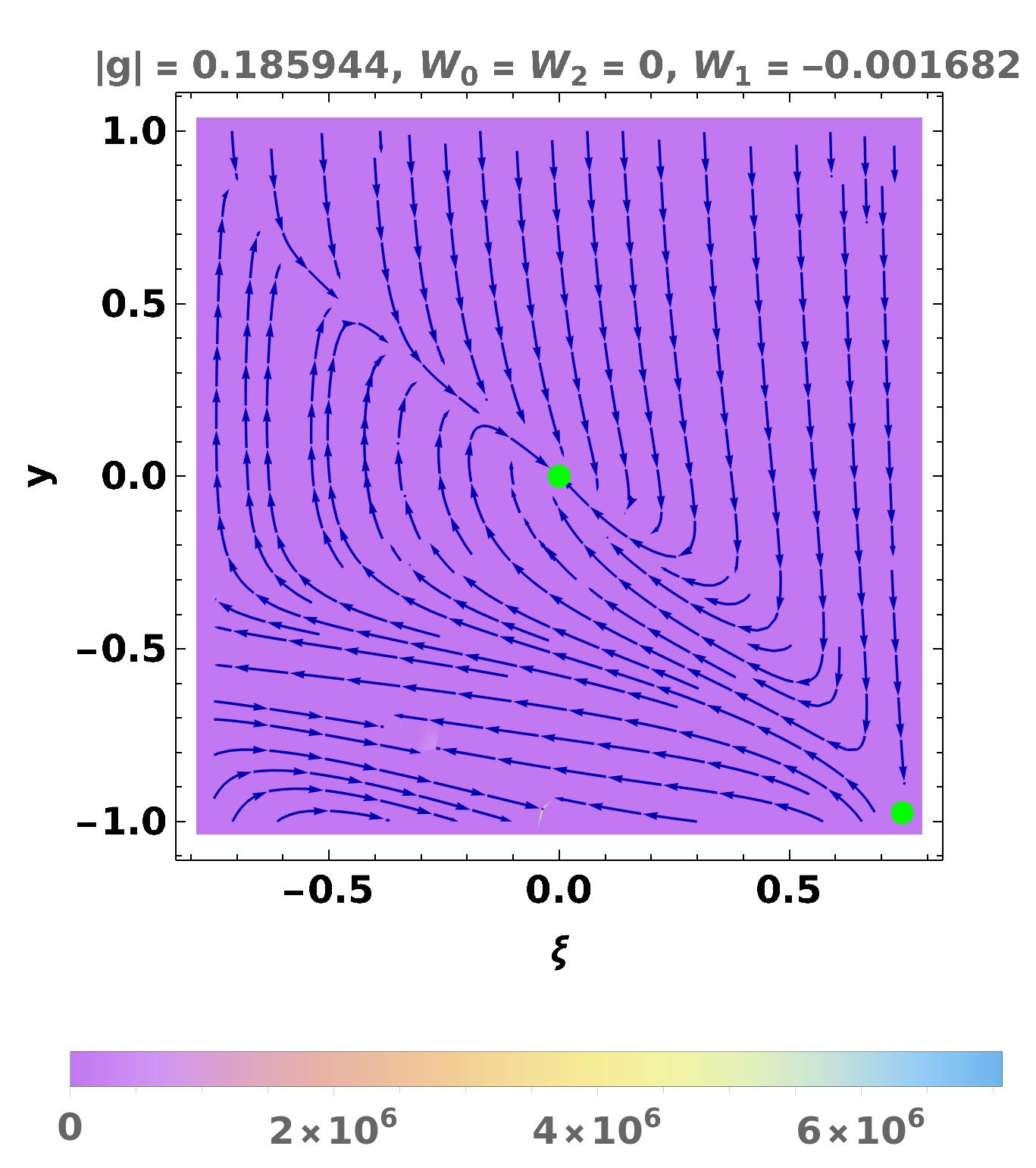
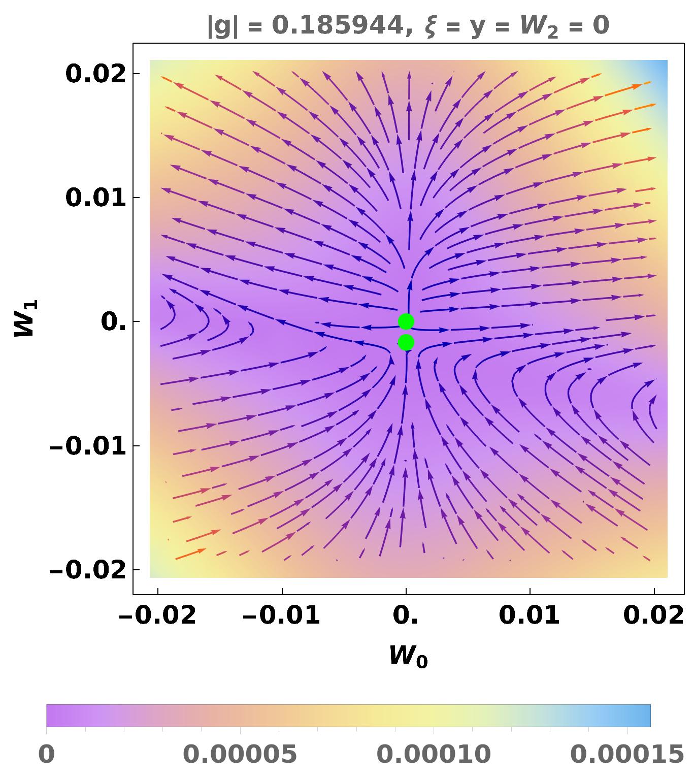
Figure 2: The RG flow diagrams for the clean system (no disorder) for N=4𝑁4N=4 and ε=0.001𝜀0.001\varepsilon=0.001. The green dots show the positions of the RG fixed points.

To analyze the stability of the non-Gaussian fixed point at |g|=246πε107N72superscript𝑔246𝜋𝜀107𝑁72|g^{*}|=\frac{24\,\sqrt{6}\,\pi\,\sqrt{\varepsilon}}{\sqrt{107\,N-72}}, we write down the linearized flow equations in its vicinity, which are:

ddl(δξδyδg)|(ξ,y,g)(δξδyδg).\displaystyle\frac{d}{dl}\left(\begin{array}[]{c}\delta\xi\\ \delta y\\ \delta g\end{array}\right)\Bigg{\rvert}_{(\xi^{*},\,y^{*},\,g^{*})}\approx\mathcal{M}\left(\begin{array}[]{c}\delta\xi\\ \delta y\\ \delta g\end{array}\right). (34)

Here l=lnμ𝑙𝜇l=-\ln\mu is the logarithmic length scale determining the RG flows towards the infrared, and

=ε107N72(722160156N107N720051846πε107N7272107N).𝜀107𝑁72722160156𝑁107𝑁720051846𝜋𝜀107𝑁7272107𝑁\displaystyle\mathcal{M}=\frac{\varepsilon}{107\,N-72}\left(\begin{array}[]{ccc}72&216&0\\ -156\,N&-107\,N-72&0\\ 0&-\frac{5184\,\sqrt{6}\,\pi\,\sqrt{\varepsilon}}{\sqrt{107\,N-72}}&72-107\,N\\ \end{array}\right)\,. (38)

The eigenvalues of \mathcal{M} are given by:

(ε,ε236±11449N2103968N+207362107N72ε).𝜀𝜀2plus-or-minus3611449superscript𝑁2103968𝑁207362107𝑁72𝜀\displaystyle\left(-\varepsilon,\,-\frac{\varepsilon}{2}-\frac{36\pm\frac{\sqrt{11449\,N^{2}-103968\,N+20736}}{2}}{107\,N-72}\,\varepsilon\right). (39)

For N=4𝑁4N=4 or N=8𝑁8N=8, the last two eigenvalues are complex conjugates of each other, and have negative real parts. The nonzero imaginary parts of the pair of complex eigenvalues (with negative real parts) indicate that the fixed point is a stable (or attractive) limit cycle in the yξ𝑦𝜉y-\xi-plane [cf. Fig. 2(a)]. For N>8𝑁8N>8, all the eigenvalues are real and negative. These results show that this non-Gaussian fixed point is stable in the infrared. On the other hand, the Gaussian fixed point is unstable, as the eigenvalues of the stability matrix are (ε/2, 0, 0)𝜀2 0 0\left(\varepsilon/2,\,0,\,0\right). Two representative RG flow diagrams are shown in Fig. 2.

IV Effect of short-range-correlated disorder

In this section, we consider the effect of adding disorder to the system of the form:

Hdis=ddx[V0(x)(ψψ)τ+V1(x)a(ψΓaψ)τ++V2(x)a<b(ψΓabψ)τ],\displaystyle H_{dis}=\int d^{d}x\,\Big{[}V_{0}(x)\,\left(\psi^{{\dagger}}\,{\psi}\right)_{\tau}+V_{1}(x)\,\sum\limits_{a}\left(\psi^{{\dagger}}\,\Gamma_{a}\,{\psi}\right)_{\tau}++V_{2}(x)\,\sum\limits_{a<b}\left(\psi^{{\dagger}}\,\Gamma_{ab}\,{\psi}\right)_{\tau}\Big{]}\,, (40)

where Vα(x)subscript𝑉𝛼𝑥V_{\alpha}(x)’s are produced by impurities or defects with and without spinor structure. We consider the case of short-range-correlated disorder such that

Vα(x)Vα(x)avg=Wαδ(xx)δαα.subscriptdelimited-⟨⟩subscript𝑉𝛼𝑥subscript𝑉superscript𝛼superscript𝑥𝑎𝑣𝑔subscript𝑊𝛼𝛿𝑥superscript𝑥subscript𝛿𝛼superscript𝛼\displaystyle\langle V_{\alpha}(x)\,V_{\alpha^{\prime}}(x^{\prime})\rangle_{avg}=W_{\alpha}\,\delta(x-x^{\prime})\,\delta_{\alpha\alpha^{\prime}}\,. (41)

The parameter Wαsubscript𝑊𝛼W_{\alpha} measures the strength of the disorder induced by the distribution of impurities. We introduce n𝑛n copies of the fields ψψi𝜓subscript𝜓𝑖\psi\to\psi_{i} with i[1,n]𝑖1𝑛i\in[1,n], and average over the disorder using Eq. (41). This is the standard treatment of disorder in the replica formalism, where the number of replicas n0𝑛0n\rightarrow 0 at the end of the computation. The replica term in the action is then given by:

Sdis=subscript𝑆disabsent\displaystyle S_{\text{dis}}= W0μεi,j=1n𝑑τ𝑑τddx(ψiψi)τ(ψjψj)τW1μεi,j=1na𝑑τ𝑑τddx(ψiΓaiψi)τ(ψjΓajψj)τsubscript𝑊0superscript𝜇𝜀superscriptsubscript𝑖𝑗1𝑛differential-d𝜏differential-dsuperscript𝜏superscript𝑑𝑑𝑥subscriptsuperscriptsubscript𝜓𝑖subscript𝜓𝑖𝜏subscriptsuperscriptsubscript𝜓𝑗subscript𝜓𝑗superscript𝜏subscript𝑊1superscript𝜇𝜀superscriptsubscript𝑖𝑗1𝑛subscript𝑎differential-d𝜏differential-dsuperscript𝜏superscript𝑑𝑑𝑥subscriptsuperscriptsubscript𝜓𝑖superscriptsubscriptΓ𝑎𝑖subscript𝜓𝑖𝜏subscriptsuperscriptsubscript𝜓𝑗superscriptsubscriptΓ𝑎𝑗subscript𝜓𝑗superscript𝜏\displaystyle-W_{0}\,\mu^{\varepsilon}\sum\limits_{i,j=1}^{n}\int d\tau\,d\tau^{\prime}\,d^{d}x\,(\psi_{i}^{{\dagger}}\,{\psi_{i}})_{\tau}\,(\psi_{j}^{{\dagger}}\,\psi_{j})_{\tau^{\prime}}-W_{1}\,\mu^{\varepsilon}\sum\limits_{i,j=1}^{n}\sum\limits_{a}\int d\tau\,d\tau^{\prime}\,d^{d}x\,({\psi_{i}}^{{\dagger}}\,\Gamma_{a}^{i}\,{\psi_{i}})_{\tau}\,(\psi_{j}^{{\dagger}}\,\Gamma_{a}^{j}\,\psi_{j})_{\tau^{\prime}}
W2μεi,j=1na<b𝑑τ𝑑τddx(ψiΓabiψi)τ(ψjΓabjψj)τ,subscript𝑊2superscript𝜇𝜀superscriptsubscript𝑖𝑗1𝑛subscript𝑎𝑏differential-d𝜏differential-dsuperscript𝜏superscript𝑑𝑑𝑥subscriptsuperscriptsubscript𝜓𝑖superscriptsubscriptΓ𝑎𝑏𝑖subscript𝜓𝑖𝜏subscriptsuperscriptsubscript𝜓𝑗superscriptsubscriptΓ𝑎𝑏𝑗subscript𝜓𝑗superscript𝜏\displaystyle-W_{2}\,\mu^{\varepsilon}\sum\limits_{i,j=1}^{n}\sum\limits_{a<b}\int d\tau\,d\tau^{\prime}\,d^{d}x\,({\psi_{i}}^{{\dagger}}\,\Gamma_{ab}^{i}\,{\psi_{i}})_{\tau}\,(\psi_{j}^{{\dagger}}\,\Gamma_{ab}^{j}\,\psi_{j})_{\tau^{\prime}}\,, (42)

where i𝑖i and j𝑗j denote the replica indices. The tree-level mass dimension of Wαsubscript𝑊𝛼W_{\alpha} is [Wα]=4ddelimited-[]subscript𝑊𝛼4𝑑[W_{\alpha}]=4-d. Let us denote the corresponding matrices by Mαsubscript𝑀𝛼M_{\alpha}, such that

(M0,M1,M2)=(𝟙Nc,Γa,Γab),subscript𝑀0subscript𝑀1subscript𝑀2subscriptdouble-struck-𝟙subscript𝑁𝑐subscriptΓ𝑎subscriptΓ𝑎𝑏\displaystyle\left(M_{0},M_{1},M_{2}\right)=(\mathbb{1}_{N_{c}},\Gamma_{a},\Gamma_{ab})\,, (43)

where Ncsubscript𝑁𝑐N_{c} is the dimensionality of the gamma matrices. For the current problem, Nc=5subscript𝑁𝑐5N_{c}=5.

IV.1 Fermion self-energy correction from disorder
Refer to caption
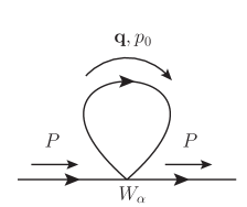
Figure 3: One-loop correction to fermion self-energy from a disorder vertex.

A sample contraction of terms leading to the one-loop correction to fermion self-energy from a disorder vertex looks like:

(ψMψ)(ψMψ)superscript𝜓𝑀𝜓superscript𝜓𝑀𝜓\displaystyle\left(\psi^{\dagger}\,M\,\psi\right)\left(\psi^{\dagger}\,M\,\psi\right) =(ψγMγ,δψδ)(ψλMλ,σψσ)=ψγ[Mγ,δ(G0)δ,λMλ,σ]ψσ.absentsubscriptsuperscript𝜓𝛾superscript𝑀𝛾𝛿subscript𝜓𝛿subscriptsuperscript𝜓𝜆superscript𝑀𝜆𝜎subscript𝜓𝜎subscriptsuperscript𝜓𝛾delimited-[]superscript𝑀𝛾𝛿subscriptsubscript𝐺0𝛿𝜆superscript𝑀𝜆𝜎subscript𝜓𝜎\displaystyle=\left(\psi^{*}_{\gamma}\,M^{\gamma,\delta}\psi_{\delta}\right)\left(\psi^{*}_{\lambda}\,M^{\lambda,\sigma}\psi_{\sigma}\right)=\psi^{*}_{\gamma}\left[M^{\gamma,\delta}\,\left(G_{0}\right)_{\delta,\lambda}\,M^{\lambda,\sigma}\right]\psi_{\sigma}\,.

Therefore, the one-loop fermion self-energy correction from disorder, shown in Fig. 3, is given by the term:

Σ1d(P)subscriptΣ1𝑑𝑃\displaystyle\Sigma_{1d}(P) =2με[W0𝐪G0(𝐪,p0)+W1a𝐪ΓaG0(𝐪,p0)Γa+W2a<b𝐪ΓabG0(𝐪,p0)Γab]absent2superscript𝜇𝜀delimited-[]subscript𝑊0subscript𝐪subscript𝐺0𝐪subscript𝑝0subscript𝑊1subscript𝑎subscript𝐪subscriptΓ𝑎subscript𝐺0𝐪subscript𝑝0subscriptΓ𝑎subscript𝑊2subscript𝑎𝑏subscript𝐪subscriptΓ𝑎𝑏subscript𝐺0𝐪subscript𝑝0subscriptΓ𝑎𝑏\displaystyle=-2\,\mu^{\varepsilon}\left[W_{0}\int_{{\bf q}}G_{0}({\bf q},p_{0})+W_{1}\sum_{a}\int_{{\bf q}}\Gamma_{a}\,G_{0}({\bf q},p_{0})\,\Gamma_{a}+W_{2}\sum_{a<b}\int_{{\bf q}}\Gamma_{ab}\,G_{0}({\bf q},p_{0})\,\Gamma_{ab}\right]
=2με[W0+NcW1+Nc(Nc1)2]𝐪iq0ξq2p02+(1ξ2)q42ip0ξq2absent2superscript𝜇𝜀delimited-[]subscript𝑊0subscript𝑁𝑐subscript𝑊1subscript𝑁𝑐subscript𝑁𝑐12subscript𝐪𝑖subscript𝑞0𝜉superscript𝑞2superscriptsubscript𝑝021superscript𝜉2superscript𝑞42𝑖subscript𝑝0𝜉superscript𝑞2\displaystyle=-2\,\mu^{\varepsilon}\left[W_{0}+N_{c}\,W_{1}+\frac{N_{c}\left(N_{c}-1\right)}{2}\right]\int_{{\bf q}}\,\frac{-i\,q_{0}-\xi\,q^{2}}{p_{0}^{2}+\left(1-\xi^{2}\right)q^{4}-2\,i\,p_{0}\,\xi\,q^{2}}
=(1+ξ2)ip0[W0+NcW1+Nc(Nc1)2]4π2(1ξ2)2ε(μ|p0|)ε+𝒪(ε0),absent1superscript𝜉2𝑖subscript𝑝0delimited-[]subscript𝑊0subscript𝑁𝑐subscript𝑊1subscript𝑁𝑐subscript𝑁𝑐124superscript𝜋2superscript1superscript𝜉22𝜀superscript𝜇subscript𝑝0𝜀𝒪superscript𝜀0\displaystyle=\frac{\left(1+\xi^{2}\right)i\,p_{0}\left[W_{0}+N_{c}\,W_{1}+\frac{N_{c}\left(N_{c}-1\right)}{2}\right]}{4\,\pi^{2}\left(1-\xi^{2}\right)^{2}\varepsilon}\left(\frac{\mu}{\sqrt{|p_{0}|}}\right)^{\varepsilon}+\mathcal{O}\left(\varepsilon^{0}\right), (44)

using Eqs. (100) and (101).

IV.2 Fermion-boson vertex correction from disorder
Refer to caption
Refer to caption
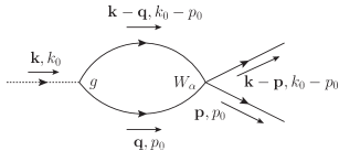
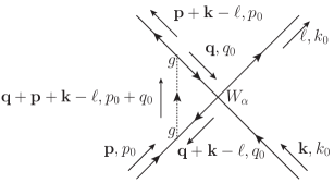
Figure 4: One-loop correction to (a) fermion-boson vertex from disorder, and (b) disorder from fermion-boson vertex.

Let us compute the one-loop fermion-boson vertex correction coming from the disorder vertices. A sample contraction of terms leading to this looks like:

ϕ(ψTΓ45ψ)(ψMψ)(ψMψ)superscriptitalic-ϕsuperscript𝜓𝑇subscriptΓ45𝜓superscript𝜓𝑀𝜓superscript𝜓𝑀𝜓\displaystyle\phi^{*}\left(\psi^{T}\,\Gamma_{45}\,\psi\right)\left(\psi^{\dagger}\,M\,\psi\right)\left(\psi^{\dagger}\,M\,\psi\right) =ϕ(ψα(Γ45)α,βψβ)(ψγMγ,δψδ)(ψλMλ,σψσ)absentsuperscriptitalic-ϕsubscript𝜓𝛼superscriptsubscriptΓ45𝛼𝛽subscript𝜓𝛽subscriptsuperscript𝜓𝛾superscript𝑀𝛾𝛿subscript𝜓𝛿subscriptsuperscript𝜓𝜆superscript𝑀𝜆𝜎subscript𝜓𝜎\displaystyle=\phi^{*}\left(\psi_{\alpha}\left(\Gamma_{45}\right)^{\alpha,\beta}\,\psi_{\beta}\right)\left(\psi^{*}_{\gamma}\,M^{\gamma,\delta}\psi_{\delta}\right)\left(\psi^{*}_{\lambda}\,M^{\lambda,\sigma}\psi_{\sigma}\right)
=ϕψδ[(G0)α,γMγ,δ(Γ45)α,β(G0)β,λMλ,σ]ψσabsentsuperscriptitalic-ϕsubscript𝜓𝛿delimited-[]subscriptsubscript𝐺0𝛼𝛾superscript𝑀𝛾𝛿superscriptsubscriptΓ45𝛼𝛽subscriptsubscript𝐺0𝛽𝜆superscript𝑀𝜆𝜎subscript𝜓𝜎\displaystyle=\phi^{*}\,\psi_{\delta}\left[\left(G_{0}\right)_{\alpha,\gamma}\,M^{\gamma,\delta}\left(\Gamma_{45}\right)^{\alpha,\beta}\,\left(G_{0}\right)_{\beta,\lambda}\,M^{\lambda,\sigma}\right]\psi_{\sigma}
=ϕψδ[(MT)δ,γ(G0T)γ,α(Γ45)α,β(G0)β,λMλ,σ]ψσ.absentsuperscriptitalic-ϕsubscript𝜓𝛿delimited-[]superscriptsuperscript𝑀𝑇𝛿𝛾subscriptsuperscriptsubscript𝐺0𝑇𝛾𝛼superscriptsubscriptΓ45𝛼𝛽subscriptsubscript𝐺0𝛽𝜆superscript𝑀𝜆𝜎subscript𝜓𝜎\displaystyle=\phi^{*}\,\psi_{\delta}\left[\left(M^{T}\right)^{\delta,\gamma}\left(G_{0}^{T}\right)_{\gamma,\alpha}\left(\Gamma_{45}\right)^{\alpha,\beta}\,\left(G_{0}\right)_{\beta,\lambda}\,M^{\lambda,\sigma}\right]\psi_{\sigma}\,.

or

ϕ(ψΓ45ψ)(ψMψ)(ψMψ)italic-ϕsuperscript𝜓subscriptΓ45superscript𝜓superscript𝜓𝑀𝜓superscript𝜓𝑀𝜓\displaystyle\phi\left(\psi^{\dagger}\,\Gamma_{45}\,\psi^{*}\right)\left(\psi^{\dagger}\,M\,\psi\right)\left(\psi^{\dagger}\,M\,\psi\right) =ϕ(ψα(Γ45)α,βψβ)(ψγMγ,δψδ)(ψλMλ,σψσ)absentitalic-ϕsubscriptsuperscript𝜓𝛼superscriptsubscriptΓ45𝛼𝛽subscriptsuperscript𝜓𝛽subscriptsuperscript𝜓𝛾superscript𝑀𝛾𝛿subscript𝜓𝛿subscriptsuperscript𝜓𝜆superscript𝑀𝜆𝜎subscript𝜓𝜎\displaystyle=\phi\left({\psi^{\dagger}}_{\alpha}\left(\Gamma_{45}\right)^{\alpha,\beta}\,\psi^{*}_{\beta}\right)\left(\psi^{*}_{\gamma}\,M^{\gamma,\delta}\psi_{\delta}\right)\left(\psi^{*}_{\lambda}\,M^{\lambda,\sigma}\psi_{\sigma}\right)
=ϕψγ[Mγ,δ(G0)δ,α(Γ45)α,β(G0)σ,βMλ,σ]ψλabsentitalic-ϕsubscriptsuperscript𝜓𝛾delimited-[]superscript𝑀𝛾𝛿subscriptsubscript𝐺0𝛿𝛼superscriptsubscriptΓ45𝛼𝛽subscriptsubscript𝐺0𝜎𝛽superscript𝑀𝜆𝜎subscriptsuperscript𝜓𝜆\displaystyle=\phi\,\psi^{*}_{\gamma}\left[M^{\gamma,\delta}\left(G_{0}\right)_{\delta,\alpha}\left(\Gamma_{45}\right)^{\alpha,\beta}\,\left(G_{0}\right)_{\sigma,\beta}\,M^{\lambda,\sigma}\right]\psi^{*}_{\lambda}
=ϕψγ[Mγ,δ(G0)δ,α(Γ45)α,β(G0T)β,σ(MT)σ,λ]ψλ.absentitalic-ϕsubscriptsuperscript𝜓𝛾delimited-[]superscript𝑀𝛾𝛿subscriptsubscript𝐺0𝛿𝛼superscriptsubscriptΓ45𝛼𝛽subscriptsuperscriptsubscript𝐺0𝑇𝛽𝜎superscriptsuperscript𝑀𝑇𝜎𝜆subscriptsuperscript𝜓𝜆\displaystyle=\phi\,\psi^{*}_{\gamma}\left[M^{\gamma,\delta}\left(G_{0}\right)_{\delta,\alpha}\left(\Gamma_{45}\right)^{\alpha,\beta}\,\left(G_{0}^{T}\right)_{\beta,\sigma}\,\left(M^{T}\right)^{\sigma,\lambda}\right]\psi^{*}_{\lambda}\,.

Therefore, we need to evaluate loop integrals of the form:

I(α)𝐼𝛼\displaystyle I(\alpha) =2gWαμ3ε2𝐪MαG0(𝐤𝐪,k0p0)Γ45G0T(𝐪,p0)MαTabsent2𝑔subscript𝑊𝛼superscript𝜇3𝜀2subscript𝐪subscript𝑀𝛼subscript𝐺0𝐤𝐪subscript𝑘0subscript𝑝0subscriptΓ45superscriptsubscript𝐺0𝑇𝐪subscript𝑝0superscriptsubscript𝑀𝛼𝑇\displaystyle=-2\,g\,W_{\alpha}\,\mu^{\frac{3\,\varepsilon}{2}}\int_{{\bf q}}M_{\alpha}\,G_{0}({\bf k}-{\bf q},k_{0}-p_{0})\,\Gamma_{45}\,G_{0}^{T}({\bf q},p_{0})\,M_{\alpha}^{T}
=2gWαμ3ε2𝐪MαG0(𝐤𝐪,k0p0)G0(𝐪,p0)Γ45MαTabsent2𝑔subscript𝑊𝛼superscript𝜇3𝜀2subscript𝐪subscript𝑀𝛼subscript𝐺0𝐤𝐪subscript𝑘0subscript𝑝0subscript𝐺0𝐪subscript𝑝0subscriptΓ45superscriptsubscript𝑀𝛼𝑇\displaystyle=-2\,g\,W_{\alpha}\,\mu^{\frac{3\,\varepsilon}{2}}\int_{{\bf q}}M_{\alpha}\,G_{0}({\bf k}-{\bf q},k_{0}-p_{0})\,G_{0}({\bf q},p_{0})\,\Gamma_{45}\,M_{\alpha}^{T}
=2gWαμ3ε2𝐪Mα[i(p0k0)ξ(𝐪𝐤)2+𝐝(𝐪𝐤)𝚪][ip0ξq2+𝐝(𝐪)𝚪]Γ45MαT[(p0k0)2+(1ξ2)(𝐪𝐤)4+2i(p0k0)ξ(𝐪𝐤)2][p02+(1ξ2)q42ip0ξq2],absent2𝑔subscript𝑊𝛼superscript𝜇3𝜀2subscript𝐪subscript𝑀𝛼delimited-[]𝑖subscript𝑝0subscript𝑘0𝜉superscript𝐪𝐤2𝐝𝐪𝐤𝚪delimited-[]𝑖subscript𝑝0𝜉superscript𝑞2𝐝𝐪𝚪subscriptΓ45subscriptsuperscript𝑀𝑇𝛼delimited-[]superscriptsubscript𝑝0subscript𝑘021superscript𝜉2superscript𝐪𝐤42𝑖subscript𝑝0subscript𝑘0𝜉superscript𝐪𝐤2delimited-[]superscriptsubscript𝑝021superscript𝜉2superscript𝑞42𝑖subscript𝑝0𝜉superscript𝑞2\displaystyle=-2\,g\,W_{\alpha}\,\mu^{\frac{3\,\varepsilon}{2}}\int_{{\bf q}}\frac{M_{\alpha}\left[i\left(p_{0}-k_{0}\right)-\xi\,\left({\bf q}-{\bf k}\right)^{2}+\mathbf{d}\left({\bf q}-{\bf k}\right)\cdot\mathbf{\Gamma}\right]\,\left[-i\,p_{0}-\xi\,q^{2}+\mathbf{d}\left(\mathbf{q}\right)\cdot\mathbf{\Gamma}\right]\Gamma_{45}\,M^{T}_{\alpha}}{\left[\left(p_{0}-k_{0}\right)^{2}+\left(1-\xi^{2}\right)\left(\mathbf{q}-\mathbf{k}\right)^{4}+2\,i\left(p_{0}-k_{0}\right)\,\xi\,\left(\mathbf{q}-\mathbf{k}\right)^{2}\right]\left[\,p_{0}^{2}+\left(1-\xi^{2}\right)q^{4}-2\,i\,p_{0}\,\xi\,q^{2}\,\right]}\,, (45)

corresponding to the one-loop vertex correction figure shown in Fig. 4(a). We set 𝐤=k0=0𝐤subscript𝑘00{\bf k}=k_{0}=0 without any loss of generality, as this will still allow us to extract the divergent part.

Using Eq. (107), for α=(0,1)𝛼01\alpha=(0,1), we get:

I(α)𝐼𝛼\displaystyle I(\alpha) =2gWαμ3ε2𝐪Mα[ip0ξq2+𝐝(𝐪𝐤)𝚪][ip0ξq2+𝐝(𝐪)𝚪]Mα[p02+(1ξ2)q4+2ip0ξ(𝐪𝐤)2][p02+(1ξ2)q42ip0ξq2]Γ45.absent2𝑔subscript𝑊𝛼superscript𝜇3𝜀2subscript𝐪subscript𝑀𝛼delimited-[]𝑖subscript𝑝0𝜉superscript𝑞2𝐝𝐪𝐤𝚪delimited-[]𝑖subscript𝑝0𝜉superscript𝑞2𝐝𝐪𝚪subscript𝑀𝛼delimited-[]superscriptsubscript𝑝021superscript𝜉2superscript𝑞42𝑖subscript𝑝0𝜉superscript𝐪𝐤2delimited-[]superscriptsubscript𝑝021superscript𝜉2superscript𝑞42𝑖subscript𝑝0𝜉superscript𝑞2subscriptΓ45\displaystyle=-2\,g\,W_{\alpha}\,\mu^{\frac{3\,\varepsilon}{2}}\int_{{\bf q}}\frac{M_{\alpha}\left[i\,p_{0}-\xi\,q^{2}+\mathbf{d}\left({\bf q}-\mathbf{k}\right)\cdot\mathbf{\Gamma}\right]\,\left[-i\,p_{0}-\xi\,q^{2}+\mathbf{d}\left(\mathbf{q}\right)\cdot\mathbf{\Gamma}\right]M_{\alpha}}{\left[p_{0}^{2}+\left(1-\xi^{2}\right)q^{4}+2\,i\,p_{0}\,\xi\,\left(\mathbf{q}-\mathbf{k}\right)^{2}\right]\left[\,p_{0}^{2}+\left(1-\xi^{2}\right)q^{4}-2\,i\,p_{0}\,\xi\,q^{2}\,\right]}\,\Gamma_{45}\,. (46)

Using Eq. (108), we get:

I(2)𝐼2\displaystyle I(2) =2gW2μ3ε2𝐪M2[ip0ξ(𝐪𝐤)2+𝐝(𝐪𝐤)𝚪][ip0ξq2+𝐝(𝐪)𝚪]M2[p02+(1ξ2)(𝐪𝐤)4+2ip0ξ(𝐪𝐤)2][p02+(1ξ2)q42ip0ξq2]Γ45.absent2𝑔subscript𝑊2superscript𝜇3𝜀2subscript𝐪subscript𝑀2delimited-[]𝑖subscript𝑝0𝜉superscript𝐪𝐤2𝐝𝐪𝐤𝚪delimited-[]𝑖subscript𝑝0𝜉superscript𝑞2𝐝𝐪𝚪subscript𝑀2delimited-[]superscriptsubscript𝑝021superscript𝜉2superscript𝐪𝐤42𝑖subscript𝑝0𝜉superscript𝐪𝐤2delimited-[]superscriptsubscript𝑝021superscript𝜉2superscript𝑞42𝑖subscript𝑝0𝜉superscript𝑞2subscriptΓ45\displaystyle=2\,g\,W_{2}\,\mu^{\frac{3\,\varepsilon}{2}}\int_{{\bf q}}\frac{M_{2}\left[i\,p_{0}-\xi\,\left({\bf q}-{\bf k}\right)^{2}+\mathbf{d}\left({\bf q}-{\bf k}\right)\cdot\mathbf{\Gamma}\right]\,\left[-i\,p_{0}-\xi\,q^{2}+\mathbf{d}\left(\mathbf{q}\right)\cdot\mathbf{\Gamma}\right]M_{2}}{\left[p_{0}^{2}+\left(1-\xi^{2}\right)\left(\mathbf{q}-\mathbf{k}\right)^{4}+2\,i\,p_{0}\,\xi\,\left(\mathbf{q}-\mathbf{k}\right)^{2}\right]\left[\,p_{0}^{2}+\left(1-\xi^{2}\right)q^{4}-2\,i\,p_{0}\,\xi\,q^{2}\,\right]}\,\Gamma_{45}\,. (47)

Let us now compute the integral

J𝐽\displaystyle J 𝐪[ip0ξq2+𝐝(𝐪)𝚪][ip0ξq2+𝐝(𝐪)𝚪][p02+(1ξ2)q4+2ip0ξq2][p02+(1ξ2)q42ip0ξq2].absentsubscript𝐪delimited-[]𝑖subscript𝑝0𝜉superscript𝑞2𝐝𝐪𝚪delimited-[]𝑖subscript𝑝0𝜉superscript𝑞2𝐝𝐪𝚪delimited-[]superscriptsubscript𝑝021superscript𝜉2superscript𝑞42𝑖subscript𝑝0𝜉superscript𝑞2delimited-[]superscriptsubscript𝑝021superscript𝜉2superscript𝑞42𝑖subscript𝑝0𝜉superscript𝑞2\displaystyle\equiv\int_{{\bf q}}\frac{\left[i\,p_{0}-\xi\,q^{2}+\mathbf{d}\left({\bf q}\right)\cdot\mathbf{\Gamma}\right]\,\left[-i\,p_{0}-\xi\,q^{2}+\mathbf{d}\left(\mathbf{q}\right)\cdot\mathbf{\Gamma}\right]}{\left[p_{0}^{2}+\left(1-\xi^{2}\right)q^{4}+2\,i\,p_{0}\,\xi\,q^{2}\right]\left[\,p_{0}^{2}+\left(1-\xi^{2}\right)q^{4}-2\,i\,p_{0}\,\xi\,q^{2}\,\right]}\,. (48)

Dropping the terms which do not contribute to vertex correction, we are left with:

Jsuperscript𝐽\displaystyle J^{\prime} 𝐪(ip0+ξq2)(ip0ξq2)+𝐝2(𝐪)[p02+(1ξ2)q4]2+4p02ξ2q4=(1+ξ2)|p0|ε28π2(1ξ2)ε+𝒪(ε0).absentsubscript𝐪𝑖subscript𝑝0𝜉superscript𝑞2𝑖subscript𝑝0𝜉superscript𝑞2superscript𝐝2𝐪superscriptdelimited-[]superscriptsubscript𝑝021superscript𝜉2superscript𝑞424superscriptsubscript𝑝02superscript𝜉2superscript𝑞41superscript𝜉2superscriptsubscript𝑝0𝜀28superscript𝜋21superscript𝜉2𝜀𝒪superscript𝜀0\displaystyle\equiv\int_{{\bf q}}\frac{-\left(i\,p_{0}+\xi\,q^{2}\right)\left(i\,p_{0}-\xi\,q^{2}\right)+{\bf d}^{2}(\mathbf{q})}{\left[\,p_{0}^{2}+\left(1-\xi^{2}\right)q^{4}\right]^{2}+4\,p_{0}^{2}\,\xi^{2}\,q^{4}}=\frac{\left(1+\xi^{2}\right)|p_{0}|^{-\frac{\varepsilon}{2}}}{8\,\pi^{2}\left(1-\xi^{2}\right)\varepsilon}+\mathcal{O}\left(\varepsilon^{0}\right). (49)

Hence, using Eqs. (100) and (101) in Eqs. (46) and (47), the divergent part of the fermion-boson vertex correction from disorder is given by:
ΓV=gμε2(1+ξ2)[W0+NcW1Nc(Nc1)W22]4π2(1ξ2)ε(μ|p0|)ε.subscriptΓ𝑉𝑔superscript𝜇𝜀21superscript𝜉2delimited-[]subscript𝑊0subscript𝑁𝑐subscript𝑊1subscript𝑁𝑐subscript𝑁𝑐1subscript𝑊224superscript𝜋21superscript𝜉2𝜀superscript𝜇subscript𝑝0𝜀\displaystyle\Gamma_{V}=-\frac{g\,\mu^{\frac{\varepsilon}{2}}\left(1+\xi^{2}\right)\left[W_{0}+N_{c}\,W_{1}-\frac{N_{c}\left(N_{c}-1\right)W_{2}}{2}\right]}{4\,\pi^{2}\left(1-\xi^{2}\right)\varepsilon}\left(\frac{\mu}{\sqrt{|p_{0}|}}\right)^{\varepsilon}\,. (50)

IV.3 Corrections to disorder vertices from fermion-boson vertex

Fig. 4(b) shows how the fermion-boson vertex can generate a one-loop correction for each disorder vertex. A sample contraction of terms leading to this looks like:

ϕ(ψTΓ45ψ)ϕ(ψΓ45ψ)(ψMψ)(ψMψ)=ϕϕ[ψα(Γ45)α,βψβ][ψγ(Γ45)γ,δψδ](ψλMλ,σψσ)(ψMψ)superscriptitalic-ϕsuperscript𝜓𝑇subscriptΓ45𝜓italic-ϕsuperscript𝜓subscriptΓ45superscript𝜓superscript𝜓𝑀𝜓superscript𝜓𝑀𝜓italic-ϕsuperscriptitalic-ϕdelimited-[]subscript𝜓𝛼superscriptsubscriptΓ45𝛼𝛽subscript𝜓𝛽delimited-[]subscriptsuperscript𝜓𝛾superscriptsubscriptΓ45𝛾𝛿subscriptsuperscript𝜓𝛿subscriptsuperscript𝜓𝜆superscript𝑀𝜆𝜎subscript𝜓𝜎superscript𝜓𝑀𝜓\displaystyle\phi^{*}\left(\psi^{T}\,\Gamma_{45}\,\psi\right)\phi\left(\psi^{\dagger}\,\Gamma_{45}\,\psi^{*}\right)\left(\psi^{\dagger}\,M\,\psi\right)\left(\psi^{\dagger}\,M\,\psi\right)=\phi\,\phi^{*}\left[\psi_{\alpha}\left(\Gamma_{45}\right)^{\alpha,\beta}\,\psi_{\beta}\right]\left[\psi^{*}_{\gamma}\left(\Gamma_{45}\right)^{\gamma,\delta}\,\psi^{*}_{\delta}\right]\left(\psi^{*}_{\lambda}\,M^{\lambda,\sigma}\psi_{\sigma}\right)\left(\psi^{\dagger}\,M\,\psi\right)
=D0[ψα(Γ45)α,βψβ](ψλMλ,σψσ)[ψγ(Γ45)γ,δψδ](ψMψ)absentsubscript𝐷0delimited-[]subscript𝜓𝛼superscriptsubscriptΓ45𝛼𝛽subscript𝜓𝛽subscriptsuperscript𝜓𝜆superscript𝑀𝜆𝜎subscript𝜓𝜎delimited-[]subscriptsuperscript𝜓𝛾superscriptsubscriptΓ45𝛾𝛿subscriptsuperscript𝜓𝛿superscript𝜓𝑀𝜓\displaystyle=D_{0}\left[\psi_{\alpha}\left(\Gamma_{45}\right)^{\alpha,\beta}\,\psi_{\beta}\right]\left(\psi^{*}_{\lambda}\,M^{\lambda,\sigma}\psi_{\sigma}\right)\left[\psi^{*}_{\gamma}\left(\Gamma_{45}\right)^{\gamma,\delta}\,\psi^{*}_{\delta}\right]\left(\psi^{\dagger}\,M\,\psi\right)
=D0[ψα(Γ45)α,β(G0)β,λMλ,σ(G0)σ,γ(Γ45)γ,δψδ](ψMψ)absentsubscript𝐷0delimited-[]subscript𝜓𝛼superscriptsubscriptΓ45𝛼𝛽subscriptsubscript𝐺0𝛽𝜆superscript𝑀𝜆𝜎subscriptsubscript𝐺0𝜎𝛾superscriptsubscriptΓ45𝛾𝛿subscriptsuperscript𝜓𝛿superscript𝜓𝑀𝜓\displaystyle=D_{0}\left[\psi_{\alpha}\left(\Gamma_{45}\right)^{\alpha,\beta}\,\left(G_{0}\right)_{\beta,\lambda}M^{\lambda,\sigma}\left(G_{0}\right)_{\sigma,\gamma}\left(\Gamma_{45}\right)^{\gamma,\delta}\,\psi^{*}_{\delta}\right]\left(\psi^{\dagger}\,M\,\psi\right)
=[ψδ{D0(Γ45)δ,γ(G0T)γ,σ(MT)σ,λ(G0T)λ,α(Γ45)α,β}ψβ](ψMψ).absentdelimited-[]subscriptsuperscript𝜓𝛿subscript𝐷0superscriptsubscriptΓ45𝛿𝛾subscriptsuperscriptsubscript𝐺0𝑇𝛾𝜎superscriptsuperscript𝑀𝑇𝜎𝜆subscriptsuperscriptsubscript𝐺0𝑇𝜆𝛼superscriptsubscriptΓ45𝛼𝛽subscript𝜓𝛽superscript𝜓𝑀𝜓\displaystyle=-\left[\psi^{*}_{\delta}\left\{D_{0}\,\left(\Gamma_{45}\right)^{\delta,\gamma}\left(G_{0}^{T}\right)_{\gamma,\sigma}\left(M^{T}\right)^{\sigma,\lambda}\left(G_{0}^{T}\right)_{\lambda,\alpha}\left(\Gamma_{45}\right)^{\alpha,\beta}\right\}\psi_{\beta}\right]\left(\psi^{\dagger}\,M\,\psi\right).

There are eight such terms.

Using Eqs. (107) and (108), The contributions will be given by integrals of the form:

4(1)2Wαg2μ2εQΓ45G0T(Q)MαTG0T(𝐪+𝐤,q0)Γ45D0(𝐪+𝐩+𝐤,p0+q0)4superscript12subscript𝑊𝛼superscript𝑔2superscript𝜇2𝜀subscript𝑄subscriptΓ45superscriptsubscript𝐺0𝑇𝑄superscriptsubscript𝑀𝛼𝑇superscriptsubscript𝐺0𝑇𝐪𝐤bold-ℓsubscript𝑞0subscriptΓ45subscript𝐷0𝐪𝐩𝐤bold-ℓsubscript𝑝0subscript𝑞0\displaystyle 4\,(-1)^{2}\,W_{\alpha}\,g^{2}\,\mu^{2\,\varepsilon}\int_{Q}\Gamma_{45}\,G_{0}^{T}(Q)\,M_{\alpha}^{T}\,G_{0}^{T}({\bf q}+{\bf k}-\bm{\ell},q_{0})\,\Gamma_{45}\,D_{0}\left({\bf q}+{\bf p}+{\bf k}-\bm{\ell},p_{0}+q_{0}\right)
=4ΩαWαg2μ2εQG0(Q)MαG0(𝐪+𝐤,q0)D0(𝐪+𝐩+𝐤,p0+q0),absent4subscriptΩ𝛼subscript𝑊𝛼superscript𝑔2superscript𝜇2𝜀subscript𝑄subscript𝐺0𝑄subscript𝑀𝛼subscript𝐺0𝐪𝐤bold-ℓsubscript𝑞0subscript𝐷0𝐪𝐩𝐤bold-ℓsubscript𝑝0subscript𝑞0\displaystyle=4\,\Omega_{\alpha}\,W_{\alpha}\,g^{2}\,\mu^{2\,\varepsilon}\int_{Q}G_{0}(Q)\,M_{\alpha}\,G_{0}({\bf q}+{\bf k}-\bm{\ell},q_{0})\,D_{0}\left({\bf q}+{\bf p}+{\bf k}-\bm{\ell},p_{0}+q_{0}\right)\,, (51)

where Ωα=1subscriptΩ𝛼1\Omega_{\alpha}=1 for α=0𝛼0\alpha=0 and α=1𝛼1\alpha=1, while Ωα=1subscriptΩ𝛼1\Omega_{\alpha}=-1 for α=2𝛼2\alpha=2. For extracting the divergent parts, we can set 𝐩=𝐤==0𝐩𝐤bold-ℓ0{\bf p}={\bf k}=\bm{\ell}=0.

Using Eqs. (100), (101), (102) and (121), the contributions for scalar, vector, and tensor disorders reduce to:

Js=4W0g2μ2εQ(iq0+ξq2)2+q4[q02+(1ξ2)q42iq0ξq2]2[iy(q0+p0)+q2],subscript𝐽𝑠4subscript𝑊0superscript𝑔2superscript𝜇2𝜀subscript𝑄superscript𝑖subscript𝑞0𝜉superscript𝑞22superscript𝑞4superscriptdelimited-[]superscriptsubscript𝑞021superscript𝜉2superscript𝑞42𝑖subscript𝑞0𝜉superscript𝑞22delimited-[]𝑖𝑦subscript𝑞0subscript𝑝0superscript𝑞2\displaystyle J_{s}=4\,W_{0}\,g^{2}\,\mu^{2\,\varepsilon}\int_{Q}\frac{\left(i\,q_{0}+\xi\,q^{2}\right)^{2}+q^{4}}{\left[q_{0}^{2}+\left(1-\xi^{2}\right)q^{4}-2\,i\,q_{0}\,\xi\,q^{2}\right]^{2}\left[i\,y\left(q_{0}+p_{0}\right)+q^{2}\right]}\,, (52)
Jv=4W1g2μ2εQ(iq0+ξq2)2(Nc2)q4Nc[q02+(1ξ2)q42iq0ξq2]2[iy(q0+p0)+q2],subscript𝐽𝑣4subscript𝑊1superscript𝑔2superscript𝜇2𝜀subscript𝑄superscript𝑖subscript𝑞0𝜉superscript𝑞22subscript𝑁𝑐2superscript𝑞4subscript𝑁𝑐superscriptdelimited-[]superscriptsubscript𝑞021superscript𝜉2superscript𝑞42𝑖subscript𝑞0𝜉superscript𝑞22delimited-[]𝑖𝑦subscript𝑞0subscript𝑝0superscript𝑞2\displaystyle J_{v}=4\,W_{1}\,g^{2}\,\mu^{2\,\varepsilon}\int_{Q}\frac{\left(i\,q_{0}+\xi\,q^{2}\right)^{2}-\frac{\left(N_{c}-2\right)q^{4}}{N_{c}}}{\left[q_{0}^{2}+\left(1-\xi^{2}\right)q^{4}-2\,i\,q_{0}\,\xi\,q^{2}\right]^{2}\left[i\,y\left(q_{0}+p_{0}\right)+q^{2}\right]}\,, (53)
Jt=4W2g2μ2εQ(iq0+ξq2)2+(Nc4)q4Nc[q02+(1ξ2)q42iq0ξq2]2[iy(q0+p0)+q2].subscript𝐽𝑡4subscript𝑊2superscript𝑔2superscript𝜇2𝜀subscript𝑄superscript𝑖subscript𝑞0𝜉superscript𝑞22subscript𝑁𝑐4superscript𝑞4subscript𝑁𝑐superscriptdelimited-[]superscriptsubscript𝑞021superscript𝜉2superscript𝑞42𝑖subscript𝑞0𝜉superscript𝑞22delimited-[]𝑖𝑦subscript𝑞0subscript𝑝0superscript𝑞2\displaystyle J_{t}=-4\,W_{2}\,g^{2}\,\mu^{2\,\varepsilon}\int_{Q}\frac{\left(i\,q_{0}+\xi\,q^{2}\right)^{2}+\frac{\left(N_{c}-4\right)q^{4}}{N_{c}}}{\left[q_{0}^{2}+\left(1-\xi^{2}\right)q^{4}-2\,i\,q_{0}\,\xi\,q^{2}\right]^{2}\left[i\,y\left(q_{0}+p_{0}\right)+q^{2}\right]}\,. (54)

On performing the integrals, we get:

Js=g2W0μεy4π2(1+yξy)2ε(μ|p0|)ε+𝒪(ε0),subscript𝐽𝑠superscript𝑔2subscript𝑊0superscript𝜇𝜀𝑦4superscript𝜋2superscript1𝑦𝜉𝑦2𝜀superscript𝜇subscript𝑝0𝜀𝒪superscript𝜀0\displaystyle J_{s}=\frac{g^{2}\,W_{0}\,\mu^{\varepsilon}\,y}{4\,\pi^{2}\left(1+y-\xi\,y\right)^{2}\,\varepsilon}\left(\frac{\mu}{\sqrt{|p_{0}|}}\right)^{\varepsilon}+\mathcal{O}\left(\varepsilon^{0}\right), (55)
Jv=g2W1με[1+2yNc(1+y)(Nc1)ξy]4π2Nc(1+yξy)2ε(μ|p0|)ε+𝒪(ε0),subscript𝐽𝑣superscript𝑔2subscript𝑊1superscript𝜇𝜀delimited-[]12𝑦subscript𝑁𝑐1𝑦subscript𝑁𝑐1𝜉𝑦4superscript𝜋2subscript𝑁𝑐superscript1𝑦𝜉𝑦2𝜀superscript𝜇subscript𝑝0𝜀𝒪superscript𝜀0\displaystyle J_{v}=\frac{g^{2}\,W_{1}\,\mu^{\varepsilon}\,\left[1+2\,y-N_{c}\,(1+y)-(N_{c}-1)\,\xi\,y\right]}{4\,\pi^{2}\,N_{c}\left(1+y-\xi\,y\right)^{2}\,\varepsilon}\left(\frac{\mu}{\sqrt{|p_{0}|}}\right)^{\varepsilon}+\mathcal{O}\left(\varepsilon^{0}\right), (56)
Jt=g2W2με[2y(Nc4+2ξ)]4π2Nc(1+yξy)2ε(μ|p0|)ε+𝒪(ε0),subscript𝐽𝑡superscript𝑔2subscript𝑊2superscript𝜇𝜀delimited-[]2𝑦subscript𝑁𝑐42𝜉4superscript𝜋2subscript𝑁𝑐superscript1𝑦𝜉𝑦2𝜀superscript𝜇subscript𝑝0𝜀𝒪superscript𝜀0\displaystyle J_{t}=\frac{g^{2}\,W_{2}\,\mu^{\varepsilon}\,\left[2-\,y\,(N_{c}-4+2\,\xi)\,\right]}{4\,\pi^{2}\,N_{c}\left(1+y-\xi\,y\right)^{2}\,\varepsilon}\left(\frac{\mu}{\sqrt{|p_{0}|}}\right)^{\varepsilon}+\mathcal{O}\left(\varepsilon^{0}\right), (57)

for the scalar, vector, and tensor disorder vertices, respectively.

IV.4 Corrections to disorder vertices from themselves

The loop corrections to the disorder lines themselves come from the fully connected contractions of

δSdis𝛿subscript𝑆dis\displaystyle\delta S_{\text{dis}} =12𝑑τ𝑑τ𝑑τ′′𝑑τ′′′dd𝐱dd𝐱i,j,k,l=1n𝒞ijkl, whereabsent12differential-d𝜏differential-dsuperscript𝜏differential-dsuperscript𝜏′′differential-dsuperscript𝜏′′′superscript𝑑𝑑𝐱superscript𝑑𝑑superscript𝐱superscriptsubscript𝑖𝑗𝑘𝑙1𝑛subscript𝒞𝑖𝑗𝑘𝑙 where\displaystyle=\frac{1}{2}\int d\tau\,d\tau^{\prime}\,d\tau^{\prime\prime}\,d\tau^{\prime\prime\prime}\,d^{d}\mathbf{x}\,d^{d}\mathbf{x}^{\prime}\sum\limits_{i,j,k,l=1}^{n}\mathcal{C}_{ijkl}\,,\text{ where}
𝒞ijklsubscript𝒞𝑖𝑗𝑘𝑙\displaystyle\mathcal{C}_{ijkl} =α,α=02WαWα(ψiMαiψi)𝐱,τ(ψjMαjψj)𝐱,τ(ψkMαkψk)𝐱,τ′′(ψlMαlψl)𝐱,τ′′′,absentsuperscriptsubscript𝛼superscript𝛼02subscript𝑊𝛼subscript𝑊superscript𝛼subscriptsuperscriptsubscript𝜓𝑖subscriptsuperscript𝑀𝑖𝛼subscript𝜓𝑖𝐱𝜏subscriptsuperscriptsubscript𝜓𝑗subscriptsuperscript𝑀𝑗𝛼subscript𝜓𝑗𝐱superscript𝜏subscriptsuperscriptsubscript𝜓𝑘subscriptsuperscript𝑀𝑘superscript𝛼subscript𝜓𝑘superscript𝐱superscript𝜏′′subscriptsuperscriptsubscript𝜓𝑙subscriptsuperscript𝑀𝑙superscript𝛼subscript𝜓𝑙superscript𝐱superscript𝜏′′′\displaystyle=\sum\limits_{\alpha,\alpha^{\prime}=0}^{2}W_{\alpha}\,W_{\alpha^{\prime}}\left(\psi_{i}^{{\dagger}}\,M^{i}_{\alpha}\,{\psi_{i}}\right)_{\mathbf{x},\tau}\left(\psi_{j}^{{\dagger}}\,M^{j}_{\alpha}\,\psi_{j}\right)_{\mathbf{x},\tau^{\prime}}\left(\psi_{k}^{{\dagger}}\,M^{k}_{\alpha^{\prime}}\,\psi_{k}\right)_{\mathbf{x}^{\prime},\tau^{\prime\prime}}\left({\psi_{l}}^{{\dagger}}\,M^{l}_{\alpha^{\prime}}\,\psi_{l}\right)_{\mathbf{x}^{\prime},\tau^{\prime\prime\prime}}\,, (58)

where we have kept track of the replica indices on the ΓΓ\Gamma-matrices. We need to consider three types of diagrams, as enumerated below:

  1. 1.

    A sample contraction of terms leading to a ZS diagram from disorder vertices takes the form:

    WαWαi,j,k,l(ψiMαiψi)𝐱,τ(ψjMαjψj)𝐱,τ(ψkMαkψk)𝐱,τ′′(ψlMαlψl)𝐱,τ′′′subscript𝑊𝛼subscript𝑊superscript𝛼subscript𝑖𝑗𝑘𝑙subscriptsubscriptsuperscript𝜓𝑖subscriptsuperscript𝑀𝑖𝛼subscript𝜓𝑖𝐱𝜏subscriptsubscriptsuperscript𝜓𝑗subscriptsuperscript𝑀𝑗𝛼subscript𝜓𝑗𝐱superscript𝜏subscriptsubscriptsuperscript𝜓𝑘subscriptsuperscript𝑀𝑘superscript𝛼subscript𝜓𝑘superscript𝐱superscript𝜏′′subscriptsubscriptsuperscript𝜓𝑙subscriptsuperscript𝑀𝑙superscript𝛼subscript𝜓𝑙superscript𝐱superscript𝜏′′′\displaystyle W_{{\alpha}}\,W_{{\alpha^{\prime}}}\sum\limits_{i,j,k,l}\left(\psi^{\dagger}_{i}\,M^{i}_{\alpha}\,\psi_{i}\right)_{\mathbf{x},\tau}\left(\psi^{\dagger}_{j}\,M^{j}_{\alpha}\,\psi_{j}\right)_{\mathbf{x},\tau^{\prime}}\left(\psi^{\dagger}_{k}\,M^{k}_{\alpha^{\prime}}\,\psi_{k}\right)_{\mathbf{x}^{\prime},\tau^{\prime\prime}}\left(\psi^{\dagger}_{l}\,M^{l}_{\alpha^{\prime}}\,\psi_{l}\right)_{\mathbf{x}^{\prime},\tau^{\prime\prime\prime}}
    =WαWαδ(ττ′′)δ(𝐱𝐱)i,j,l(ψiMαiψi)𝐱,τTr(G0jMαjG0jMαj)𝐱,τ(ψlMαlψl)𝐱,τ′′′absentsubscript𝑊𝛼subscript𝑊superscript𝛼𝛿superscript𝜏superscript𝜏′′𝛿𝐱superscript𝐱subscript𝑖𝑗𝑙subscriptsubscriptsuperscript𝜓𝑖subscriptsuperscript𝑀𝑖𝛼subscript𝜓𝑖𝐱𝜏Trsubscriptsuperscriptsubscript𝐺0𝑗superscriptsubscript𝑀𝛼𝑗superscriptsubscript𝐺0𝑗subscriptsuperscript𝑀𝑗superscript𝛼𝐱superscript𝜏subscriptsubscriptsuperscript𝜓𝑙subscriptsuperscript𝑀𝑙superscript𝛼subscript𝜓𝑙𝐱superscript𝜏′′′\displaystyle=-W_{\alpha}\,W_{\alpha^{\prime}}\,\delta(\tau^{\prime}-\tau^{\prime\prime})\,\delta(\mathbf{x}-\mathbf{x}^{\prime})\sum\limits_{i,j,l}\left(\psi^{\dagger}_{i}\,M^{i}_{\alpha}\,\psi_{i}\right)_{\mathbf{x},\tau}\text{Tr}\left(G_{0}^{j}\,M_{\alpha}^{j}\,G_{0}^{j}\,M^{j}_{\alpha^{\prime}}\right)_{\mathbf{x},\tau^{\prime}}\left(\psi^{\dagger}_{l}\,M^{l}_{\alpha^{\prime}}\,\psi_{l}\right)_{\mathbf{x},\tau^{\prime\prime\prime}}
    =nTr(G0MαG0Mα)𝐱,τWαWαδ(τ′′τ′′′)δ(𝐱𝐱)i,j(ψiMαiψi)τ(ψjMαjψj)𝐱,τ′′′.absent𝑛Trsubscriptsubscript𝐺0subscript𝑀𝛼subscript𝐺0subscript𝑀superscript𝛼𝐱superscript𝜏subscript𝑊𝛼subscript𝑊superscript𝛼𝛿superscript𝜏′′superscript𝜏′′′𝛿𝐱superscript𝐱subscript𝑖𝑗subscriptsubscriptsuperscript𝜓𝑖superscriptsubscript𝑀𝛼𝑖subscript𝜓𝑖𝜏subscriptsubscriptsuperscript𝜓𝑗subscriptsuperscript𝑀𝑗superscript𝛼subscript𝜓𝑗𝐱superscript𝜏′′′\displaystyle=-n\,\text{Tr}\left(G_{0}\,M_{\alpha}\,G_{0}\,M_{\alpha^{\prime}}\right)_{\mathbf{x},\tau^{\prime}}W_{\alpha}\,W_{\alpha^{\prime}}\,\delta(\tau^{\prime\prime}-\tau^{\prime\prime\prime})\,\delta(\mathbf{x}-\mathbf{x}^{\prime})\sum\limits_{i,j}\left(\psi^{\dagger}_{i}\,M_{\alpha}^{i}\,\psi_{i}\right)_{\tau}\left(\psi^{\dagger}_{j}\,M^{j}_{\alpha^{\prime}}\,\psi_{j}\right)_{\mathbf{x},\tau^{\prime\prime\prime}}. (59)

    Hence, a ZS diagram comes with a factor of n𝑛n, which vanishes upon taking the replica limit n0𝑛0n\rightarrow 0.

  2. 2.

    For the VC diagrams, a sample contraction of terms looks like:

    WαWαi,j,k,l(ψiMαiψi)𝐱,τ(ψjMαjψj)𝐱,τ(ψkMαkψk)𝐱,τ′′(ψlMαlψl)𝐱,τ′′′subscript𝑊𝛼subscript𝑊superscript𝛼subscript𝑖𝑗𝑘𝑙subscriptsubscriptsuperscript𝜓𝑖superscriptsubscript𝑀𝛼𝑖subscript𝜓𝑖𝐱𝜏subscriptsubscriptsuperscript𝜓𝑗superscriptsubscript𝑀𝛼𝑗subscript𝜓𝑗𝐱superscript𝜏subscriptsubscriptsuperscript𝜓𝑘superscriptsubscript𝑀superscript𝛼𝑘subscript𝜓𝑘superscript𝐱superscript𝜏′′subscriptsubscriptsuperscript𝜓𝑙superscriptsubscript𝑀superscript𝛼𝑙subscript𝜓𝑙superscript𝐱superscript𝜏′′′\displaystyle W_{\alpha}\,W_{\alpha^{\prime}}\sum\limits_{i,j,k,l}\left(\psi^{\dagger}_{i}\,M_{\alpha}^{i}\,\psi_{i}\right)_{\mathbf{x},\tau}\left(\psi^{\dagger}_{j}\,M_{\alpha}^{j}\,\psi_{j}\right)_{\mathbf{x},\tau^{\prime}}\left(\psi^{\dagger}_{k}\,M_{\alpha^{\prime}}^{k}\,\psi_{k}\right)_{\mathbf{x}^{\prime},\tau^{\prime\prime}}\left(\psi^{\dagger}_{l}\,M_{\alpha^{\prime}}^{l}\,\psi_{l}\right)_{\mathbf{x}^{\prime},\tau^{\prime\prime\prime}}
    =WαWαδ(ττ′′)δ(ττ′′′)δ(𝐱𝐱)i,j(ψiMαiψj)𝐱,τ(ψjMαjG0jMαjG0jMαbψb)𝐱,τ′′.absentsubscript𝑊𝛼subscript𝑊superscript𝛼𝛿superscript𝜏superscript𝜏′′𝛿superscript𝜏superscript𝜏′′′𝛿𝐱superscript𝐱subscript𝑖𝑗subscriptsubscriptsuperscript𝜓𝑖subscriptsuperscript𝑀𝑖𝛼subscript𝜓𝑗𝐱𝜏subscriptsubscriptsuperscript𝜓𝑗superscriptsubscript𝑀superscript𝛼𝑗superscriptsubscript𝐺0𝑗subscriptsuperscript𝑀𝑗𝛼superscriptsubscript𝐺0𝑗superscriptsubscript𝑀superscript𝛼𝑏subscript𝜓𝑏𝐱superscript𝜏′′\displaystyle=W_{\alpha}\,W_{\alpha^{\prime}}\,\delta(\tau^{\prime}-\tau^{\prime\prime})\,\delta(\tau^{\prime}-\tau^{\prime\prime\prime})\,\delta(\mathbf{x}-\mathbf{x}^{\prime})\sum\limits_{i,j}\left(\psi^{\dagger}_{i}\,M^{i}_{\alpha}\,\psi_{j}\right)_{\mathbf{x},\tau}\left(\psi^{\dagger}_{j}\,M_{\alpha^{\prime}}^{j}\,G_{0}^{j}\,M^{j}_{\alpha}\,G_{0}^{j}\,M_{\alpha^{\prime}}^{b}\,\psi_{b}\right)_{\mathbf{x},\tau^{\prime\prime}}. (60)

    A VC diagram with two Wαsubscript𝑊𝛼W_{\alpha} vertices can emerge in 8 distinct way. Gathering all the factors, and setting the external frequency p0=0subscript𝑝00p_{0}=0 for easily extracting the divergent part, we find a correction to the
    (a) scalar vertex from

    Γ00VC=4W02μ2ε𝐪G0(𝐪,p0)G0(𝐪,p0)=(1+ξ2)W02με2π2(1ξ2)2ε(μ|p0|)ε.superscriptsubscriptΓ00𝑉𝐶4superscriptsubscript𝑊02superscript𝜇2𝜀subscript𝐪subscript𝐺0𝐪subscript𝑝0subscript𝐺0𝐪subscript𝑝01superscript𝜉2superscriptsubscript𝑊02superscript𝜇𝜀2superscript𝜋2superscript1superscript𝜉22𝜀superscript𝜇subscript𝑝0𝜀\displaystyle\Gamma_{00}^{VC}=4\,W_{0}^{2}\,\mu^{2\varepsilon}\int_{{\bf q}}G_{0}({\bf q},p_{0})\,G_{0}({\bf q},p_{0})=\frac{\left(1+\xi^{2}\right)W_{0}^{2}\,\mu^{\varepsilon}}{2\,\pi^{2}\left(1-\xi^{2}\right)^{2}\varepsilon}\left(\frac{\mu}{\sqrt{\left|p_{0}\right|}}\right)^{\varepsilon}. (61)

    (b) vector vertex from

    Γ11VCsuperscriptsubscriptΓ11𝑉𝐶\displaystyle\Gamma_{11}^{VC} =4W12μ2εΓaiΓbj𝐪G0j(𝐪,p0)ΓajG0j(𝐪,p0)Γbjabsent4superscriptsubscript𝑊12superscript𝜇2𝜀superscriptsubscriptΓ𝑎𝑖superscriptsubscriptΓ𝑏𝑗subscript𝐪superscriptsubscript𝐺0𝑗𝐪subscript𝑝0superscriptsubscriptΓ𝑎𝑗superscriptsubscript𝐺0𝑗𝐪subscript𝑝0superscriptsubscriptΓ𝑏𝑗\displaystyle=4\,W_{1}^{2}\,\mu^{2\varepsilon}\,\Gamma_{a}^{i}\,\Gamma_{b}^{j}\int_{{\bf q}}G_{0}^{j}({\bf q},p_{0})\,\Gamma_{a}^{j}\,G_{0}^{j}({\bf q},p_{0})\,\Gamma_{b}^{j}
    =(Nc2)(2Nc1+ξ2)W12μεΓaiΓaj2π2(1ξ2)2ε(μ|p0|)ε.absentsubscript𝑁𝑐22subscript𝑁𝑐1superscript𝜉2superscriptsubscript𝑊12superscript𝜇𝜀superscriptsubscriptΓ𝑎𝑖superscriptsubscriptΓ𝑎𝑗2superscript𝜋2superscript1superscript𝜉22𝜀superscript𝜇subscript𝑝0𝜀\displaystyle=-\frac{\left(N_{c}-2\right)\left(\frac{2}{N_{c}}-1+\xi^{2}\right)W_{1}^{2}\,\mu^{\varepsilon}\,\Gamma_{a}^{i}\,\Gamma_{a}^{j}}{2\,\pi^{2}\left(1-\xi^{2}\right)^{2}\varepsilon}\left(\frac{\mu}{\sqrt{\left|p_{0}\right|}}\right)^{\varepsilon}. (62)

    (c) tensor vertex from

    Γ22VCsuperscriptsubscriptΓ22𝑉𝐶\displaystyle\Gamma_{22}^{VC} =4W22μ2εΓabiΓcdj𝐪G0j(𝐪,p0)ΓabjG0j(𝐪,p0)Γcdjabsent4superscriptsubscript𝑊22superscript𝜇2𝜀superscriptsubscriptΓ𝑎𝑏𝑖superscriptsubscriptΓ𝑐𝑑𝑗subscript𝐪superscriptsubscript𝐺0𝑗𝐪subscript𝑝0superscriptsubscriptΓ𝑎𝑏𝑗superscriptsubscript𝐺0𝑗𝐪subscript𝑝0superscriptsubscriptΓ𝑐𝑑𝑗\displaystyle=4\,W_{2}^{2}\,\mu^{2\varepsilon}\,\Gamma_{ab}^{i}\,\Gamma_{cd}^{j}\int_{{\bf q}}G_{0}^{j}({\bf q},p_{0})\,\Gamma_{ab}^{j}\,G_{0}^{j}({\bf q},p_{0})\,\Gamma_{cd}^{j}
    =(1+ξ24Nc)(Nc29Nc+16)W22μεΓabiΓabj4π2(1ξ2)2ε(μ|p0|)ε.absent1superscript𝜉24subscript𝑁𝑐superscriptsubscript𝑁𝑐29subscript𝑁𝑐16superscriptsubscript𝑊22superscript𝜇𝜀superscriptsubscriptΓ𝑎𝑏𝑖superscriptsubscriptΓ𝑎𝑏𝑗4superscript𝜋2superscript1superscript𝜉22𝜀superscript𝜇subscript𝑝0𝜀\displaystyle=\frac{\left(1+\xi^{2}-\frac{4}{N_{c}}\right)\left(N_{c}^{2}-9N_{c}+16\right)W_{2}^{2}\,\mu^{\varepsilon}\,\Gamma_{ab}^{i}\,\Gamma_{ab}^{j}}{4\,\pi^{2}\left(1-\xi^{2}\right)^{2}\varepsilon}\left(\frac{\mu}{\sqrt{\left|p_{0}\right|}}\right)^{\varepsilon}. (63)

    VC diagrams with mixed lines can emerge in one of two ways, each of which corrects a different bare vertex and comes with a combinatorial factor of 444. The contributions can be listed as:
    (a)

    Γ01VCsuperscriptsubscriptΓ01𝑉𝐶\displaystyle\Gamma_{01}^{VC} =4W0W1μ2εΓbj𝐪G0j(𝐪,p0)G0j(𝐪,p0)Γbj=(1+ξ2)NcW0W1με2π2(1ξ2)2ε(μ|p0|)ε,absent4subscript𝑊0subscript𝑊1superscript𝜇2𝜀superscriptsubscriptΓ𝑏𝑗subscript𝐪superscriptsubscript𝐺0𝑗𝐪subscript𝑝0superscriptsubscript𝐺0𝑗𝐪subscript𝑝0superscriptsubscriptΓ𝑏𝑗1superscript𝜉2subscript𝑁𝑐subscript𝑊0subscript𝑊1superscript𝜇𝜀2superscript𝜋2superscript1superscript𝜉22𝜀superscript𝜇subscript𝑝0𝜀\displaystyle=4\,W_{0}\,W_{1}\,\mu^{2\varepsilon}\,\Gamma_{b}^{j}\int_{{\bf q}}G_{0}^{j}({\bf q},p_{0})\,G_{0}^{j}({\bf q},p_{0})\,\Gamma_{b}^{j}=\frac{\left(1+\xi^{2}\right)N_{c}\,W_{0}\,W_{1}\,\mu^{\varepsilon}}{2\,\pi^{2}\left(1-\xi^{2}\right)^{2}\varepsilon}\left(\frac{\mu}{\sqrt{\left|p_{0}\right|}}\right)^{\varepsilon}, (64)

    correcting the scalar vertex.

    (b)

    Γ10VC=4W0W1μ2εΓai𝐪G0j(𝐪,p0)ΓajG0j(𝐪,p0)=(2Nc1+ξ2)W0W1μεΓaiΓaj2π2(1ξ2)2ε(μ|p0|)ε,superscriptsubscriptΓ10𝑉𝐶4subscript𝑊0subscript𝑊1superscript𝜇2𝜀superscriptsubscriptΓ𝑎𝑖subscript𝐪superscriptsubscript𝐺0𝑗𝐪subscript𝑝0superscriptsubscriptΓ𝑎𝑗superscriptsubscript𝐺0𝑗𝐪subscript𝑝02subscript𝑁𝑐1superscript𝜉2subscript𝑊0subscript𝑊1superscript𝜇𝜀superscriptsubscriptΓ𝑎𝑖superscriptsubscriptΓ𝑎𝑗2superscript𝜋2superscript1superscript𝜉22𝜀superscript𝜇subscript𝑝0𝜀\displaystyle\Gamma_{10}^{VC}=4\,W_{0}\,W_{1}\,\mu^{2\varepsilon}\,\Gamma_{a}^{i}\,\int_{{\bf q}}G_{0}^{j}({\bf q},p_{0})\,\Gamma_{a}^{j}\,G_{0}^{j}({\bf q},p_{0})=\frac{\left(\frac{2}{N_{c}}-1+\xi^{2}\right)\,W_{0}\,W_{1}\,\mu^{\varepsilon}\,\Gamma_{a}^{i}\,\Gamma_{a}^{j}}{2\,\pi^{2}\left(1-\xi^{2}\right)^{2}\varepsilon}\left(\frac{\mu}{\sqrt{\left|p_{0}\right|}}\right)^{\varepsilon}, (65)

    correcting the vector vertex.

    (c)

    Γ02VC=4W0W2μ2εΓabj𝐪G0j(𝐪,p0)G0j(𝐪,p0)Γabj=(1+ξ2)Nc(Nc1)W0W2με4π2(1ξ2)2ε(μ|p0|)ε,superscriptsubscriptΓ02𝑉𝐶4subscript𝑊0subscript𝑊2superscript𝜇2𝜀superscriptsubscriptΓ𝑎𝑏𝑗subscript𝐪superscriptsubscript𝐺0𝑗𝐪subscript𝑝0superscriptsubscript𝐺0𝑗𝐪subscript𝑝0superscriptsubscriptΓ𝑎𝑏𝑗1superscript𝜉2subscript𝑁𝑐subscript𝑁𝑐1subscript𝑊0subscript𝑊2superscript𝜇𝜀4superscript𝜋2superscript1superscript𝜉22𝜀superscript𝜇subscript𝑝0𝜀\displaystyle\Gamma_{02}^{VC}=4\,W_{0}\,W_{2}\,\mu^{2\varepsilon}\,\Gamma_{ab}^{j}\int_{{\bf q}}G_{0}^{j}({\bf q},p_{0})\,G_{0}^{j}({\bf q},p_{0})\,\Gamma_{ab}^{j}=\frac{\left(1+\xi^{2}\right)N_{c}\left(N_{c}-1\right)\,W_{0}\,W_{2}\,\mu^{\varepsilon}}{4\,\pi^{2}\left(1-\xi^{2}\right)^{2}\varepsilon}\left(\frac{\mu}{\sqrt{\left|p_{0}\right|}}\right)^{\varepsilon}, (66)

    correcting the scalar vertex.

    (d)

    Γ20VC=4W0W2μ2εΓabi𝐪G0j(𝐪,p0)ΓabjG0j(𝐪,p0)=(1+ξ24/Nc)W0W2μεΓabiΓabj2π2(1ξ2)2ε(μ|p0|)ε,superscriptsubscriptΓ20𝑉𝐶4subscript𝑊0subscript𝑊2superscript𝜇2𝜀superscriptsubscriptΓ𝑎𝑏𝑖subscript𝐪superscriptsubscript𝐺0𝑗𝐪subscript𝑝0superscriptsubscriptΓ𝑎𝑏𝑗superscriptsubscript𝐺0𝑗𝐪subscript𝑝01superscript𝜉24subscript𝑁𝑐subscript𝑊0subscript𝑊2superscript𝜇𝜀superscriptsubscriptΓ𝑎𝑏𝑖superscriptsubscriptΓ𝑎𝑏𝑗2superscript𝜋2superscript1superscript𝜉22𝜀superscript𝜇subscript𝑝0𝜀\displaystyle\Gamma_{20}^{VC}=4\,W_{0}\,W_{2}\,\mu^{2\varepsilon}\,\Gamma_{ab}^{i}\int_{{\bf q}}G_{0}^{j}({\bf q},p_{0})\,\Gamma_{ab}^{j}\,G_{0}^{j}({\bf q},p_{0})=\frac{\left(1+\xi^{2}-4/N_{c}\right)W_{0}\,W_{2}\,\mu^{\varepsilon}\,\Gamma_{ab}^{i}\,\Gamma_{ab}^{j}}{2\,\pi^{2}\left(1-\xi^{2}\right)^{2}\varepsilon}\left(\frac{\mu}{\sqrt{\left|p_{0}\right|}}\right)^{\varepsilon}, (67)

    correcting the tensor vertex.

    (e)

    Γ12VCsuperscriptsubscriptΓ12𝑉𝐶\displaystyle\Gamma_{12}^{VC} =4W1W2μ2εΓaiΓcdj𝐪G0j(𝐪,p0)ΓajG0j(𝐪,p0)Γcdjabsent4subscript𝑊1subscript𝑊2superscript𝜇2𝜀superscriptsubscriptΓ𝑎𝑖superscriptsubscriptΓ𝑐𝑑𝑗subscript𝐪superscriptsubscript𝐺0𝑗𝐪subscript𝑝0superscriptsubscriptΓ𝑎𝑗superscriptsubscript𝐺0𝑗𝐪subscript𝑝0superscriptsubscriptΓ𝑐𝑑𝑗\displaystyle=4\,W_{1}\,W_{2}\,\mu^{2\varepsilon}\,\Gamma_{a}^{i}\,\Gamma_{cd}^{j}\int_{{\bf q}}G_{0}^{j}({\bf q},p_{0})\,\Gamma_{a}^{j}\,G_{0}^{j}({\bf q},p_{0})\,\Gamma_{cd}^{j}
    =(Nc4)(Nc1)(2Nc1+ξ2)W1W2μεΓaiΓaj4π2(1ξ2)2ε(μ|p0|)ε,absentsubscript𝑁𝑐4subscript𝑁𝑐12subscript𝑁𝑐1superscript𝜉2subscript𝑊1subscript𝑊2superscript𝜇𝜀superscriptsubscriptΓ𝑎𝑖superscriptsubscriptΓ𝑎𝑗4superscript𝜋2superscript1superscript𝜉22𝜀superscript𝜇subscript𝑝0𝜀\displaystyle=\frac{\left(N_{c}-4\right)\left(N_{c}-1\right)\left(\frac{2}{N_{c}}-1+\xi^{2}\right)W_{1}\,W_{2}\,\mu^{\varepsilon}\,\Gamma_{a}^{i}\,\Gamma_{a}^{j}}{4\,\pi^{2}\left(1-\xi^{2}\right)^{2}\varepsilon}\left(\frac{\mu}{\sqrt{\left|p_{0}\right|}}\right)^{\varepsilon}, (68)

    correcting the vector vertex.

    (f)

    Γ21VCsuperscriptsubscriptΓ21𝑉𝐶\displaystyle\Gamma_{21}^{VC} =4W1W2μ2εΓabiΓcj𝐪G0j(𝐪,p0)ΓabjG0j(𝐪,p0)Γcjabsent4subscript𝑊1subscript𝑊2superscript𝜇2𝜀superscriptsubscriptΓ𝑎𝑏𝑖superscriptsubscriptΓ𝑐𝑗subscript𝐪superscriptsubscript𝐺0𝑗𝐪subscript𝑝0superscriptsubscriptΓ𝑎𝑏𝑗superscriptsubscript𝐺0𝑗𝐪subscript𝑝0superscriptsubscriptΓ𝑐𝑗\displaystyle=4\,W_{1}\,W_{2}\,\mu^{2\varepsilon}\,\Gamma_{ab}^{i}\,\Gamma_{c}^{j}\int_{{\bf q}}G_{0}^{j}({\bf q},p_{0})\,\Gamma_{ab}^{j}\,G_{0}^{j}({\bf q},p_{0})\,\Gamma_{c}^{j}
    =(Nc4)(1+ξ24Nc)W1W2μεΓabiΓabj2π2(1ξ2)2ε(μ|p0|)ε,absentsubscript𝑁𝑐41superscript𝜉24subscript𝑁𝑐subscript𝑊1subscript𝑊2superscript𝜇𝜀superscriptsubscriptΓ𝑎𝑏𝑖superscriptsubscriptΓ𝑎𝑏𝑗2superscript𝜋2superscript1superscript𝜉22𝜀superscript𝜇subscript𝑝0𝜀\displaystyle=\frac{\left(N_{c}-4\right)\left(1+\xi^{2}-\frac{4}{N_{c}}\right)W_{1}\,W_{2}\,\mu^{\varepsilon}\,\Gamma_{ab}^{i}\,\Gamma_{ab}^{j}}{2\,\pi^{2}\left(1-\xi^{2}\right)^{2}\varepsilon}\left(\frac{\mu}{\sqrt{\left|p_{0}\right|}}\right)^{\varepsilon}, (69)

    correcting the tensor vertex.

  3. 3.

    For the BCS and ZS diagrams, sample contractions look like:

    WαWαi,j,k,l(ψiMαiψi)τ(ψjMαjψj)τ(ψkMαkψk)τ′′(ψlMαlψl)τ′′′subscript𝑊𝛼subscript𝑊superscript𝛼subscript𝑖𝑗𝑘𝑙subscriptsubscriptsuperscript𝜓𝑖superscriptsubscript𝑀𝛼𝑖subscript𝜓𝑖𝜏subscriptsubscriptsuperscript𝜓𝑗superscriptsubscript𝑀superscript𝛼𝑗subscript𝜓𝑗superscript𝜏subscriptsubscriptsuperscript𝜓𝑘superscriptsubscript𝑀𝛼𝑘subscript𝜓𝑘superscript𝜏′′subscriptsubscriptsuperscript𝜓𝑙superscriptsubscript𝑀superscript𝛼𝑙subscript𝜓𝑙superscript𝜏′′′\displaystyle W_{\alpha}\,W_{\alpha^{\prime}}\sum\limits_{i,j,k,l}\left(\psi^{\dagger}_{i}\,M_{\alpha}^{i}\,\psi_{i}\right)_{\tau}\left(\psi^{\dagger}_{j}\,M_{\alpha^{\prime}}^{j}\,\psi_{j}\right)_{\tau^{\prime}}\left(\psi^{\dagger}_{k}\,M_{\alpha}^{k}\,\psi_{k}\right)_{\tau^{\prime\prime}}\left(\psi^{\dagger}_{l}\,M_{\alpha^{\prime}}^{l}\,\psi_{l}\right)_{\tau^{\prime\prime\prime}}
    =WαWαδ(ττ)δ(τ′′τ′′′)i,j(ψiMαiG0iMαiψi)τ(ψjMαjG0jMαjψj)τ′′,absentsubscript𝑊𝛼subscript𝑊superscript𝛼𝛿𝜏superscript𝜏𝛿superscript𝜏′′superscript𝜏′′′subscript𝑖𝑗subscriptsubscriptsuperscript𝜓𝑖superscriptsubscript𝑀𝛼𝑖superscriptsubscript𝐺0𝑖superscriptsubscript𝑀superscript𝛼𝑖subscript𝜓𝑖𝜏subscriptsubscriptsuperscript𝜓𝑗superscriptsubscript𝑀𝛼𝑗superscriptsubscript𝐺0𝑗superscriptsubscript𝑀superscript𝛼𝑗subscript𝜓𝑗superscript𝜏′′\displaystyle=W_{\alpha}\,W_{\alpha^{\prime}}\,\delta(\tau-\tau^{\prime})\,\delta(\tau^{\prime\prime}-\tau^{\prime\prime\prime})\sum\limits_{i,j}\left(\psi^{\dagger}_{i}\,M_{\alpha}^{i}\,G_{0}^{i}\,M_{\alpha^{\prime}}^{i}\,\psi_{i}\right)_{\tau}\left(\psi^{\dagger}_{j}\,M_{\alpha}^{j}\,G_{0}^{j}\,M_{\alpha^{\prime}}^{j}\,\psi_{j}\right)_{\tau^{\prime\prime}}, (70)

    and

    WαWαδ(ττ)δ(τ′′τ′′′)i,j(ψiMαiG0iMαiψa)τ(ψjMαjG0jMαjψj)τ′′,subscript𝑊𝛼subscript𝑊superscript𝛼𝛿𝜏superscript𝜏𝛿superscript𝜏′′superscript𝜏′′′subscript𝑖𝑗subscriptsubscriptsuperscript𝜓𝑖superscriptsubscript𝑀𝛼𝑖superscriptsubscript𝐺0𝑖superscriptsubscript𝑀superscript𝛼𝑖subscript𝜓𝑎𝜏subscriptsubscriptsuperscript𝜓𝑗superscriptsubscript𝑀superscript𝛼𝑗superscriptsubscript𝐺0𝑗superscriptsubscript𝑀𝛼𝑗subscript𝜓𝑗superscript𝜏′′\displaystyle W_{\alpha}\,W_{\alpha^{\prime}}\,\delta(\tau-\tau^{\prime})\,\delta(\tau^{\prime\prime}-\tau^{\prime\prime\prime})\sum\limits_{i,j}\left(\psi^{\dagger}_{i}\,M_{\alpha}^{i}\,G_{0}^{i}\,M_{\alpha^{\prime}}^{i}\,\psi_{a}\right)_{\tau}\left(\psi^{\dagger}_{j}\,M_{\alpha^{\prime}}^{j}\,G_{0}^{j}\,M_{\alpha}^{j}\,\psi_{j}\right)_{\tau^{\prime\prime}}, (71)

    respectively.

    Each of these one-loop corrections comes with an overall factor of 222, and the final answer depends on the nature of the internal disorder lines. The contributions, combining the BCS and ZS’ counterparts, can be listed as:
    (a)

    Π00BCS+ZS=4W02μ2ε𝐪G0i(𝐪,p0)G0j(𝐪,p0)=[ξ22π2(1ξ2)2ε+ΓaiΓaj2π2(1ξ2)2Ncε]W02με(μ|p0|)ε,superscriptsubscriptΠ00𝐵𝐶𝑆𝑍superscript𝑆4superscriptsubscript𝑊02superscript𝜇2𝜀subscript𝐪superscriptsubscript𝐺0𝑖𝐪subscript𝑝0superscriptsubscript𝐺0𝑗𝐪subscript𝑝0delimited-[]superscript𝜉22superscript𝜋2superscript1superscript𝜉22𝜀superscriptsubscriptΓ𝑎𝑖superscriptsubscriptΓ𝑎𝑗2superscript𝜋2superscript1superscript𝜉22subscript𝑁𝑐𝜀superscriptsubscript𝑊02superscript𝜇𝜀superscript𝜇subscript𝑝0𝜀\displaystyle\Pi_{00}^{BCS+ZS^{\prime}}=4\,W_{0}^{2}\,\mu^{2\varepsilon}\int_{{\bf q}}G_{0}^{i}({\bf q},p_{0})\,G_{0}^{j}({\bf q},p_{0})=\left[\frac{\xi^{2}}{2\,\pi^{2}\left(1-\xi^{2}\right)^{2}\varepsilon}+\frac{\Gamma_{a}^{i}\,\Gamma_{a}^{j}}{2\,\pi^{2}\left(1-\xi^{2}\right)^{2}N_{c}\,\varepsilon}\right]W_{0}^{2}\,\mu^{\varepsilon}\left(\frac{\mu}{\sqrt{\left|p_{0}\right|}}\right)^{\varepsilon}, (72)

    correcting both the scalar and vector vertices.

    (b)

    Π11BCS+ZSsuperscriptsubscriptΠ11𝐵𝐶𝑆𝑍superscript𝑆\displaystyle\Pi_{11}^{BCS+ZS^{\prime}} =2W12μ2ε𝐪ΓaiG0i(𝐪,p0)Γbi[Γaj(𝐪,p0)G0j(𝐪,p0)Γbj+ΓbjG0j(𝐪,p0)Γaj]absent2superscriptsubscript𝑊12superscript𝜇2𝜀subscript𝐪superscriptsubscriptΓ𝑎𝑖superscriptsubscript𝐺0𝑖𝐪subscript𝑝0superscriptsubscriptΓ𝑏𝑖delimited-[]superscriptsubscriptΓ𝑎𝑗𝐪subscript𝑝0superscriptsubscript𝐺0𝑗𝐪subscript𝑝0superscriptsubscriptΓ𝑏𝑗superscriptsubscriptΓ𝑏𝑗superscriptsubscript𝐺0𝑗𝐪subscript𝑝0superscriptsubscriptΓ𝑎𝑗\displaystyle=2\,W_{1}^{2}\,\mu^{2\varepsilon}\int_{{\bf q}}\Gamma_{a}^{i}\,G_{0}^{i}({\bf q},p_{0})\,\Gamma_{b}^{i}\left[\Gamma_{a}^{j}({\bf q},p_{0})\,G_{0}^{j}({\bf q},p_{0})\,\Gamma_{b}^{j}+\Gamma_{b}^{j}\,G_{0}^{j}({\bf q},p_{0})\,\Gamma_{a}^{j}\right]
    =[ξ2Nc2π2(1ξ2)2ε+(3Nc2)ΓaiΓaj2π2(1ξ2)2Ncε]W12με(μ|p0|)ε,absentdelimited-[]superscript𝜉2subscript𝑁𝑐2superscript𝜋2superscript1superscript𝜉22𝜀3subscript𝑁𝑐2superscriptsubscriptΓ𝑎𝑖superscriptsubscriptΓ𝑎𝑗2superscript𝜋2superscript1superscript𝜉22subscript𝑁𝑐𝜀superscriptsubscript𝑊12superscript𝜇𝜀superscript𝜇subscript𝑝0𝜀\displaystyle=\left[\frac{\xi^{2}\,N_{c}}{2\,\pi^{2}\left(1-\xi^{2}\right)^{2}\varepsilon}+\frac{\left(3\,N_{c}-2\right)\Gamma_{a}^{i}\,\Gamma_{a}^{j}}{2\,\pi^{2}\left(1-\xi^{2}\right)^{2}N_{c}\,\varepsilon}\right]W_{1}^{2}\,\mu^{\varepsilon}\left(\frac{\mu}{\sqrt{\left|p_{0}\right|}}\right)^{\varepsilon}, (73)

    correcting both the scalar and vector vertices.

    (c)

    Π22BCS+ZSsuperscriptsubscriptΠ22𝐵𝐶𝑆𝑍superscript𝑆\displaystyle\Pi_{22}^{BCS+ZS^{\prime}} =2W22μ2ε𝐪ΓabiG0i(𝐪,p0)Γcdi[ΓabjG0j(𝐪,p0)Γcdj+ΓcdjG0j(𝐪,p0)Γabj]absent2superscriptsubscript𝑊22superscript𝜇2𝜀subscript𝐪superscriptsubscriptΓ𝑎𝑏𝑖superscriptsubscript𝐺0𝑖𝐪subscript𝑝0superscriptsubscriptΓ𝑐𝑑𝑖delimited-[]superscriptsubscriptΓ𝑎𝑏𝑗superscriptsubscript𝐺0𝑗𝐪subscript𝑝0superscriptsubscriptΓ𝑐𝑑𝑗superscriptsubscriptΓ𝑐𝑑𝑗superscriptsubscript𝐺0𝑗𝐪subscript𝑝0superscriptsubscriptΓ𝑎𝑏𝑗\displaystyle=2\,W_{2}^{2}\,\mu^{2\varepsilon}\int_{{\bf q}}\Gamma_{ab}^{i}\,G_{0}^{i}({\bf q},p_{0})\,\Gamma_{cd}^{i}\left[\Gamma_{ab}^{j}\,G_{0}^{j}({\bf q},p_{0})\,\Gamma_{cd}^{j}+\Gamma_{cd}^{j}\,G_{0}^{j}({\bf q},p_{0})\,\Gamma_{ab}^{j}\right]
    =[6+13ξ22π2(1ξ2)2ε+(17+15ξ2)ΓaiΓaj5π2(1ξ2)2ε3ξ2ΓabiΓabjπ2(1ξ2)2ε]W22με(μ|p0|)ε,absentdelimited-[]613superscript𝜉22superscript𝜋2superscript1superscript𝜉22𝜀1715superscript𝜉2superscriptsubscriptΓ𝑎𝑖superscriptsubscriptΓ𝑎𝑗5superscript𝜋2superscript1superscript𝜉22𝜀3superscript𝜉2superscriptsubscriptΓ𝑎𝑏𝑖superscriptsubscriptΓ𝑎𝑏𝑗superscript𝜋2superscript1superscript𝜉22𝜀superscriptsubscript𝑊22superscript𝜇𝜀superscript𝜇subscript𝑝0𝜀\displaystyle=\left[\frac{6+13\,\xi^{2}}{2\,\pi^{2}\left(1-\xi^{2}\right)^{2}\varepsilon}+\frac{\left(17+15\,\xi^{2}\right)\Gamma_{a}^{i}\,\Gamma_{a}^{j}}{5\,\pi^{2}\left(1-\xi^{2}\right)^{2}\varepsilon}-\frac{3\,\xi^{2}\,\Gamma_{ab}^{i}\,\Gamma_{ab}^{j}}{\pi^{2}\left(1-\xi^{2}\right)^{2}\varepsilon}\right]W_{2}^{2}\,\mu^{\varepsilon}\left(\frac{\mu}{\sqrt{\left|p_{0}\right|}}\right)^{\varepsilon}, (74)

    correcting the scalar, vector, and tensor vertices.

    (d)

    Π01BCS+ZS+Π10BCS+ZSsuperscriptsubscriptΠ01𝐵𝐶𝑆𝑍superscript𝑆superscriptsubscriptΠ10𝐵𝐶𝑆𝑍superscript𝑆\displaystyle\Pi_{01}^{BCS+ZS^{\prime}}+\Pi_{10}^{BCS+ZS^{\prime}} =4W0W1μ2ε𝐪G0i(𝐪,p0)Γai[G0j(𝐪,p0)Γaj+ΓajG0j(𝐪,p0)]absent4subscript𝑊0subscript𝑊1superscript𝜇2𝜀subscript𝐪superscriptsubscript𝐺0𝑖𝐪subscript𝑝0superscriptsubscriptΓ𝑎𝑖delimited-[]superscriptsubscript𝐺0𝑗𝐪subscript𝑝0superscriptsubscriptΓ𝑎𝑗superscriptsubscriptΓ𝑎𝑗superscriptsubscript𝐺0𝑗𝐪subscript𝑝0\displaystyle=4\,W_{0}\,W_{1}\,\mu^{2\varepsilon}\int_{{\bf q}}G_{0}^{i}({\bf q},p_{0})\,\Gamma_{a}^{i}\left[G_{0}^{j}({\bf q},p_{0})\,\Gamma_{a}^{j}+\Gamma_{a}^{j}\,G_{0}^{j}({\bf q},p_{0})\right]
    =[ξ2π2(1ξ2)2ε+ΓaiΓajπ2(1ξ2)2Ncε]W0W1με(μ|p0|)ε,absentdelimited-[]superscript𝜉2superscript𝜋2superscript1superscript𝜉22𝜀superscriptsubscriptΓ𝑎𝑖superscriptsubscriptΓ𝑎𝑗superscript𝜋2superscript1superscript𝜉22subscript𝑁𝑐𝜀subscript𝑊0subscript𝑊1superscript𝜇𝜀superscript𝜇subscript𝑝0𝜀\displaystyle=\left[\frac{\xi^{2}}{\pi^{2}\left(1-\xi^{2}\right)^{2}\varepsilon}+\frac{\Gamma_{a}^{i}\,\Gamma_{a}^{j}}{\pi^{2}\left(1-\xi^{2}\right)^{2}N_{c}\,\varepsilon}\right]W_{0}\,W_{1}\,\mu^{\varepsilon}\left(\frac{\mu}{\sqrt{\left|p_{0}\right|}}\right)^{\varepsilon}, (75)

    correcting both the scalar and vector vertices.

    (e)

    Π02BCS+ZS+Π20BCS+ZSsuperscriptsubscriptΠ02𝐵𝐶𝑆𝑍superscript𝑆superscriptsubscriptΠ20𝐵𝐶𝑆𝑍superscript𝑆\displaystyle\Pi_{02}^{BCS+ZS^{\prime}}+\Pi_{20}^{BCS+ZS^{\prime}} =4W0W2μ2ε𝐪G0i(𝐪,p0)Γabi[G0j(𝐪,p0)Γabj+ΓabjG0j(𝐪,p0)]absent4subscript𝑊0subscript𝑊2superscript𝜇2𝜀subscript𝐪superscriptsubscript𝐺0𝑖𝐪subscript𝑝0superscriptsubscriptΓ𝑎𝑏𝑖delimited-[]superscriptsubscript𝐺0𝑗𝐪subscript𝑝0superscriptsubscriptΓ𝑎𝑏𝑗superscriptsubscriptΓ𝑎𝑏𝑗superscriptsubscript𝐺0𝑗𝐪subscript𝑝0\displaystyle=4\,W_{0}\,W_{2}\,\mu^{2\varepsilon}\int_{{\bf q}}G_{0}^{i}({\bf q},p_{0})\,\Gamma_{ab}^{i}\left[G_{0}^{j}({\bf q},p_{0})\,\Gamma_{ab}^{j}+\Gamma_{ab}^{j}\,G_{0}^{j}({\bf q},p_{0})\right]
    =(3/10+ξ2)ΓabiΓabjπ2(1ξ2)2εW0W2με(μ|p0|)ε,absent310superscript𝜉2superscriptsubscriptΓab𝑖superscriptsubscriptΓab𝑗superscript𝜋2superscript1superscript𝜉22𝜀subscript𝑊0subscript𝑊2superscript𝜇𝜀superscript𝜇subscript𝑝0𝜀\displaystyle=\frac{\left(3/10+\xi^{2}\right)\Gamma_{\text{ab}}^{i}\,\Gamma_{\text{ab}}^{j}}{\pi^{2}\left(1-\xi^{2}\right)^{2}\varepsilon}\,W_{0}\,W_{2}\,\mu^{\varepsilon}\left(\frac{\mu}{\sqrt{\left|p_{0}\right|}}\right)^{\varepsilon}, (76)

    correcting the tensor vertex.

    (f)

    Π12BCS+ZS+Π21BCS+ZSsuperscriptsubscriptΠ12𝐵𝐶𝑆𝑍superscript𝑆superscriptsubscriptΠ21𝐵𝐶𝑆𝑍superscript𝑆\displaystyle\Pi_{12}^{BCS+ZS^{\prime}}+\Pi_{21}^{BCS+ZS^{\prime}} =4W1W2μ2ε𝐪ΓaiG0i(𝐪,p0)Γbci[ΓajG0j(𝐪,p0)Γbcj+ΓbcjG0j(𝐪,p0)Γaj]absent4subscript𝑊1subscript𝑊2superscript𝜇2𝜀subscript𝐪superscriptsubscriptΓ𝑎𝑖superscriptsubscript𝐺0𝑖𝐪subscript𝑝0superscriptsubscriptΓ𝑏𝑐𝑖delimited-[]superscriptsubscriptΓ𝑎𝑗superscriptsubscript𝐺0𝑗𝐪subscript𝑝0superscriptsubscriptΓ𝑏𝑐𝑗superscriptsubscriptΓ𝑏𝑐𝑗superscriptsubscript𝐺0𝑗𝐪subscript𝑝0superscriptsubscriptΓ𝑎𝑗\displaystyle=4\,W_{1}\,W_{2}\,\mu^{2\varepsilon}\int_{{\bf q}}\Gamma_{a}^{i}\,G_{0}^{i}({\bf q},p_{0})\,\Gamma_{bc}^{i}\left[\Gamma_{a}^{j}\,G_{0}^{j}({\bf q},p_{0})\,\Gamma_{bc}^{j}+\Gamma_{bc}^{j}\,G_{0}^{j}({\bf q},p_{0})\,\Gamma_{a}^{j}\right]
    =34+15ξ210π2(1ξ2)2εW1W2με(μ|p0|)ε,absent3415superscript𝜉210superscript𝜋2superscript1superscript𝜉22𝜀subscript𝑊1subscript𝑊2superscript𝜇𝜀superscript𝜇subscript𝑝0𝜀\displaystyle=\frac{34+15\,\xi^{2}}{10\,\pi^{2}\left(1-\xi^{2}\right)^{2}\varepsilon}\,W_{1}\,W_{2}\,\mu^{\varepsilon}\left(\frac{\mu}{\sqrt{\left|p_{0}\right|}}\right)^{\varepsilon}, (77)

    correcting the tensor vertex.

For calculational convenience, the final results have been gathered and tabulated in Tables 1 and 2.

Coupling W0subscript𝑊0W_{0} W1subscript𝑊1W_{1} W2subscript𝑊2W_{2}
W0subscript𝑊0W_{0} Z7,1(1+ξ2)W02π2(1ξ2)2subscript𝑍711superscript𝜉2subscript𝑊02superscript𝜋2superscript1superscript𝜉22Z_{7,1}\rightarrow\frac{-\left(1+\xi^{2}\right)W_{0}}{2\,\pi^{2}\left(1-\xi^{2}\right)^{2}} Z7,1(1+ξ2)NcW12π2(1ξ2)2subscript𝑍711superscript𝜉2subscript𝑁𝑐subscript𝑊12superscript𝜋2superscript1superscript𝜉22Z_{7,1}\rightarrow-\frac{\left(1+\xi^{2}\right)N_{c}\,W_{1}}{2\,\pi^{2}\left(1-\xi^{2}\right)^{2}} Z7,1(1+ξ2)Nc(Nc1)W24π2(1ξ2)2subscript𝑍711superscript𝜉2subscript𝑁𝑐subscript𝑁𝑐1subscript𝑊24superscript𝜋2superscript1superscript𝜉22Z_{7,1}\rightarrow-\frac{\left(1+\xi^{2}\right)N_{c}\left(N_{c}-1\right)W_{2}}{4\,\pi^{2}\left(1-\xi^{2}\right)^{2}}
W1subscript𝑊1W_{1} Z8,1(2Nc1+ξ2)W02π2(1ξ2)2subscript𝑍812subscript𝑁𝑐1superscript𝜉2subscript𝑊02superscript𝜋2superscript1superscript𝜉22Z_{8,1}\rightarrow\frac{\left(\frac{2}{N_{c}}-1+\xi^{2}\right)W_{0}}{2\,\pi^{2}\left(1-\xi^{2}\right)^{2}} Z8,1(Nc2)(2Nc1+ξ2)W12π2(1ξ2)2subscript𝑍81subscript𝑁𝑐22subscript𝑁𝑐1superscript𝜉2subscript𝑊12superscript𝜋2superscript1superscript𝜉22Z_{8,1}\rightarrow\frac{\left(N_{c}-2\right)\left(\frac{2}{N_{c}}-1+\xi^{2}\right)W_{1}}{2\,\pi^{2}\left(1-\xi^{2}\right)^{2}} Z8,1(Nc4)(Nc1)(2Nc1+ξ2)W24π2(1ξ2)2subscript𝑍81subscript𝑁𝑐4subscript𝑁𝑐12subscript𝑁𝑐1superscript𝜉2subscript𝑊24superscript𝜋2superscript1superscript𝜉22Z_{8,1}\rightarrow-\frac{\left(N_{c}-4\right)\left(N_{c}-1\right)\left(\frac{2}{N_{c}}-1+\xi^{2}\right)W_{2}}{4\,\pi^{2}\left(1-\xi^{2}\right)^{2}}
W2subscript𝑊2W_{2} Z9,1(1+ξ24Nc)W02π2(1ξ2)2subscript𝑍911superscript𝜉24subscript𝑁𝑐subscript𝑊02superscript𝜋2superscript1superscript𝜉22Z_{9,1}\rightarrow-\frac{\left(1+\xi^{2}-\frac{4}{N_{c}}\right)W_{0}}{2\,\pi^{2}\left(1-\xi^{2}\right)^{2}} Z9,1(Nc4)(1+ξ24Nc)W12π2(1ξ2)2εsubscript𝑍91subscript𝑁𝑐41superscript𝜉24subscript𝑁𝑐subscript𝑊12superscript𝜋2superscript1superscript𝜉22𝜀Z_{9,1}\rightarrow-\frac{\left(N_{c}-4\right)\left(1+\xi^{2}-\frac{4}{N_{c}}\right)W_{1}}{2\,\pi^{2}\left(1-\xi^{2}\right)^{2}\varepsilon} Z9,1(1+ξ24Nc)(Nc29Nc+16)W24π2(1ξ2)2subscript𝑍911superscript𝜉24subscript𝑁𝑐superscriptsubscript𝑁𝑐29subscript𝑁𝑐16subscript𝑊24superscript𝜋2superscript1superscript𝜉22Z_{9,1}\rightarrow-\frac{\left(1+\xi^{2}-\frac{4}{N_{c}}\right)\left(N_{c}^{2}-9N_{c}+16\right)W_{2}}{4\,\pi^{2}\left(1-\xi^{2}\right)^{2}}
Table 1: Contributions to Zn,1subscript𝑍𝑛1Z_{n,1} (for n=7, 8, 9𝑛789n=7,\,8,\,9) from the disorder-only VC diagrams.
Coupling W0subscript𝑊0W_{0} W1subscript𝑊1W_{1} W2subscript𝑊2W_{2}
W0subscript𝑊0W_{0} Z7,1ξ2W02π2(1ξ2)2subscript𝑍71superscript𝜉2subscript𝑊02superscript𝜋2superscript1superscript𝜉22Z_{7,1}\rightarrow-\frac{\xi^{2}\,W_{0}}{2\,\pi^{2}\left(1-\xi^{2}\right)^{2}} Z8,1W022π2(1ξ2)2NcW1subscript𝑍81superscriptsubscript𝑊022superscript𝜋2superscript1superscript𝜉22subscript𝑁𝑐subscript𝑊1Z_{8,1}\rightarrow-\frac{W_{0}^{2}}{2\,\pi^{2}\left(1-\xi^{2}\right)^{2}N_{c}\,W_{1}} Z7,1ξ2W1π2(1ξ2)2subscript𝑍71superscript𝜉2subscript𝑊1superscript𝜋2superscript1superscript𝜉22Z_{7,1}\rightarrow-\frac{\xi^{2}\,W_{1}}{\pi^{2}\left(1-\xi^{2}\right)^{2}} Z8,1W0π2(1ξ2)2Ncsubscript𝑍81subscript𝑊0superscript𝜋2superscript1superscript𝜉22subscript𝑁𝑐Z_{8,1}\rightarrow-\frac{W_{0}}{\pi^{2}\left(1-\xi^{2}\right)^{2}N_{c}} Z9,1(ξ2+310)W0π2(1ξ2)2subscript𝑍91superscript𝜉2310subscript𝑊0superscript𝜋2superscript1superscript𝜉22Z_{9,1}\rightarrow-\frac{\left(\xi^{2}+\frac{3}{10}\right)W_{0}}{\pi^{2}\left(1-\xi^{2}\right)^{2}}
W1subscript𝑊1W_{1} included in (W0,W1)subscript𝑊0subscript𝑊1(W_{0},\,W_{1}) cell Z7,1ξ2NcW122π2(1ξ2)2W0subscript𝑍71superscript𝜉2subscript𝑁𝑐superscriptsubscript𝑊122superscript𝜋2superscript1superscript𝜉22subscript𝑊0Z_{7,1}\rightarrow-\frac{\xi^{2}\,N_{c}\,W_{1}^{2}}{2\,\pi^{2}\left(1-\xi^{2}\right)^{2}W_{0}} Z8,1(3Nc2)W22π2(1ξ2)2Ncsubscript𝑍813subscript𝑁𝑐2subscript𝑊22superscript𝜋2superscript1superscript𝜉22subscript𝑁𝑐Z_{8,1}\rightarrow-\frac{\left(3\,N_{c}-2\right)W_{2}}{2\,\pi^{2}\left(1-\xi^{2}\right)^{2}N_{c}} Z9,1(34+15ξ2)W110π2(1ξ2)2subscript𝑍913415superscript𝜉2subscript𝑊110superscript𝜋2superscript1superscript𝜉22Z_{9,1}\rightarrow-\frac{\left(34+15\,\xi^{2}\right)W_{1}}{10\,\pi^{2}\left(1-\xi^{2}\right)^{2}}
W2subscript𝑊2W_{2} included in (W0,W2)subscript𝑊0subscript𝑊2(W_{0},\,W_{2}) cell included in (W1,W2)subscript𝑊1subscript𝑊2(W_{1},\,W_{2}) cell Z7,1(6+13ξ2)W222π2(1ξ2)2W0subscript𝑍71613superscript𝜉2superscriptsubscript𝑊222superscript𝜋2superscript1superscript𝜉22subscript𝑊0Z_{7,1}\rightarrow-\frac{\left(6+13\,\xi^{2}\right)W_{2}^{2}}{2\,\pi^{2}\left(1-\xi^{2}\right)^{2}W_{0}} Z8,1(17+15ξ2)W225π2(1ξ2)2W1subscript𝑍811715superscript𝜉2superscriptsubscript𝑊225superscript𝜋2superscript1superscript𝜉22subscript𝑊1Z_{8,1}\rightarrow-\frac{\left(17+15\,\xi^{2}\right)W_{2}^{2}}{5\,\pi^{2}\left(1-\xi^{2}\right)^{2}W_{1}} Z9,13ξ2W2π2(1ξ2)2subscript𝑍913superscript𝜉2subscript𝑊2superscript𝜋2superscript1superscript𝜉22Z_{9,1}\rightarrow\frac{3\,\xi^{2}\,W_{2}}{\pi^{2}\left(1-\xi^{2}\right)^{2}}
Table 2: Contributions to Zn,1subscript𝑍𝑛1Z_{n,1} (for n=7, 8, 9𝑛789n=7,\,8,\,9) from the BCS and ZS diagrams.

IV.5 RG equations

The counterterm action for the disorder part is given by:

𝒮CTdis=subscriptsuperscript𝒮dis𝐶𝑇absent\displaystyle{\mathcal{S}}^{\text{dis}}_{CT}= μεi,jp0k0(m=14𝐩m)(2π)dδd(𝐩1+𝐩3𝐩2𝐩4)superscript𝜇𝜀subscript𝑖𝑗subscriptsubscript𝑝0subscriptsubscript𝑘0superscriptsubscriptproduct𝑚14subscriptsubscript𝐩𝑚superscript2𝜋𝑑superscript𝛿𝑑subscript𝐩1subscript𝐩3subscript𝐩2subscript𝐩4\displaystyle-\mu^{\varepsilon}\sum\limits_{i,j}\int_{p_{0}}\int_{k_{0}}\left(\prod\limits_{m=1}^{4}\int_{{\bf p}_{m}}\right)\left(2\,\pi\right)^{d}\,\delta^{d}\left({\bf p}_{1}+{\bf p}_{3}-{\bf p}_{2}-{\bf p}_{4}\right)
×[A7W0{ψi(𝐩1,p0)ψi(𝐩2,p0)}{ψj(𝐩3,k0)ψj(𝐩4,k0)}\displaystyle\hskip 42.67912pt\times\Big{[}\,A_{7}\,W_{0}\left\{\psi_{i}^{{\dagger}}({\bf p}_{1},p_{0})\,{\psi_{i}}({\bf p}_{2},p_{0})\right\}\left\{\psi_{j}^{{\dagger}}({\bf p}_{3},k_{0})\,{\psi_{j}}({\bf p}_{4},k_{0})\right\}
+A8W1a{ψi(𝐩1,p0)Γaiψi(𝐩2,p0)}{ψj(𝐩3,k0)Γajψj(𝐩4,k0)}subscript𝐴8subscript𝑊1subscript𝑎superscriptsubscript𝜓𝑖subscript𝐩1subscript𝑝0superscriptsubscriptΓ𝑎𝑖subscript𝜓𝑖subscript𝐩2subscript𝑝0superscriptsubscript𝜓𝑗subscript𝐩3subscript𝑘0superscriptsubscriptΓ𝑎𝑗subscript𝜓𝑗subscript𝐩4subscript𝑘0\displaystyle\hskip 56.9055pt+A_{8}\,W_{1}\sum\limits_{a}\left\{\psi_{i}^{{\dagger}}({\bf p}_{1},p_{0})\,\Gamma_{a}^{i}\,{\psi_{i}}({\bf p}_{2},p_{0})\right\}\left\{\psi_{j}^{{\dagger}}({\bf p}_{3},k_{0})\,\Gamma_{a}^{j}\,{\psi_{j}}({\bf p}_{4},k_{0})\right\}
+A9W2a<b{ψi(𝐩1,p0)Γabiψi(𝐩2,p0)}{ψj(𝐩3,k0)Γabjψj(𝐩4,k0)}],\displaystyle\hskip 56.9055pt+A_{9}\,W_{2}\sum\limits_{a<b}\left\{\psi_{i}^{{\dagger}}({\bf p}_{1},p_{0})\,\Gamma_{ab}^{i}\,{\psi_{i}}({\bf p}_{2},p_{0})\right\}\left\{\psi_{j}^{{\dagger}}({\bf p}_{3},k_{0})\,\Gamma_{ab}^{j}\,{\psi_{j}}({\bf p}_{4},k_{0})\right\}\,\Big{]}\,, (78)

where An=Zn1=λ=1Zn,λελsubscript𝐴𝑛subscript𝑍𝑛1superscriptsubscript𝜆1subscript𝑍𝑛𝜆superscript𝜀𝜆A_{n}=Z_{n}-1=\sum\limits_{\lambda=1}^{\infty}\frac{Z_{n,\lambda}}{\varepsilon^{\lambda}} as before.

Adding these counterterms, the disorder part of the renormalized action is:

𝒮rendis=subscriptsuperscript𝒮dis𝑟𝑒𝑛absent\displaystyle{\mathcal{S}}^{\text{dis}}_{ren}= i,jp0Bk0B(m=14𝐩mB)(2π)dδd(𝐩1B+𝐩3B𝐩2B𝐩4B)subscript𝑖𝑗subscriptsubscript𝑝subscript0𝐵subscriptsubscript𝑘subscript0𝐵superscriptsubscriptproduct𝑚14subscriptsubscript𝐩subscript𝑚𝐵superscript2𝜋𝑑superscript𝛿𝑑subscript𝐩subscript1𝐵subscript𝐩subscript3𝐵subscript𝐩subscript2𝐵subscript𝐩subscript4𝐵\displaystyle-\sum\limits_{i,j}\int_{p_{0_{B}}}\int_{k_{0_{B}}}\left(\prod\limits_{m=1}^{4}\int_{{\bf p}_{m_{B}}}\right)\left(2\,\pi\right)^{d}\,\delta^{d}\left({\bf p}_{1_{B}}+{\bf p}_{3_{B}}-{\bf p}_{2_{B}}-{\bf p}_{4_{B}}\right)
×[W0B{ψiB(𝐩1B,p0B)ψiB(𝐩2B,p0B)}{ψjB(𝐩3B,k0B)ψjB(𝐩4B,k0B)}\displaystyle\hskip 28.45274pt\times\Big{[}\,{W_{0}}_{B}\left\{{\psi_{i}}_{B}^{{\dagger}}({\bf p}_{1_{B}},p_{0_{B}})\,{\psi_{i}}_{B}({\bf p}_{2_{B}},p_{0_{B}})\right\}\left\{{\psi_{j}}_{B}^{{\dagger}}({\bf p}_{3_{B}},k_{0_{B}})\,{\psi_{j}}_{B}({\bf p}_{4_{B}},k_{0_{B}})\right\}
+W1Ba{ψiB(𝐩1B,p0B)ΓaiψiB(𝐩2B,p0B)}{ψjB(𝐩3B,k0B)ΓajψjB(𝐩4B,k0B)}subscriptsubscript𝑊1𝐵subscript𝑎superscriptsubscriptsubscript𝜓𝑖𝐵subscript𝐩subscript1𝐵subscript𝑝subscript0𝐵superscriptsubscriptΓ𝑎𝑖subscriptsubscript𝜓𝑖𝐵subscript𝐩subscript2𝐵subscript𝑝subscript0𝐵superscriptsubscriptsubscript𝜓𝑗𝐵subscript𝐩subscript3𝐵subscript𝑘subscript0𝐵superscriptsubscriptΓ𝑎𝑗subscriptsubscript𝜓𝑗𝐵subscript𝐩subscript4𝐵subscript𝑘subscript0𝐵\displaystyle\hskip 42.67912pt+{W_{1}}_{B}\sum\limits_{a}\left\{{\psi_{i}}_{B}^{{\dagger}}({\bf p}_{1_{B}},p_{0_{B}})\,\Gamma_{a}^{i}\,{\psi_{i}}_{B}({\bf p}_{2_{B}},p_{0_{B}})\right\}\left\{{\psi_{j}}_{B}^{{\dagger}}({\bf p}_{3_{B}},k_{0_{B}})\,\Gamma_{a}^{j}\,{\psi_{j}}_{B}({\bf p}_{4_{B}},k_{0_{B}})\right\}
+W2Ba<b{ψiB(𝐩1B,p0B)ΓabiψiB(𝐩2B,p0B)}{ψjB(𝐩3B,k0B)ΓabjψjB(𝐩4B,k0B)}],\displaystyle\hskip 42.67912pt+{W_{2}}_{B}\sum\limits_{a<b}\left\{{\psi_{i}}_{B}^{{\dagger}}({\bf p}_{1_{B}},p_{0_{B}})\,\Gamma_{ab}^{i}\,{\psi_{i}}_{B}({\bf p}_{2_{B}},p_{0_{B}})\right\}\left\{{\psi_{j}}_{B}^{{\dagger}}({\bf p}_{3_{B}},k_{0_{B}})\,\Gamma_{ab}^{j}\,{\psi_{j}}_{B}({\bf p}_{4_{B}},k_{0_{B}})\right\}\Big{]}\,, (79)

where, in addition to Eq. (III.2), we now have:

W0B=Z7μεZ2d/2W0,W1B=Z8μεZ2d/2W1,W2B=Z9μεZ2d/2W2.formulae-sequencesubscriptsubscript𝑊0𝐵subscript𝑍7superscript𝜇𝜀superscriptsubscript𝑍2𝑑2subscript𝑊0formulae-sequencesubscriptsubscript𝑊1𝐵subscript𝑍8superscript𝜇𝜀superscriptsubscript𝑍2𝑑2subscript𝑊1subscriptsubscript𝑊2𝐵subscript𝑍9superscript𝜇𝜀superscriptsubscript𝑍2𝑑2subscript𝑊2\displaystyle{W_{0}}_{B}=\frac{Z_{7}\,\mu^{\varepsilon}}{Z_{2}^{d/2}}\,W_{0}\,,\quad{W_{1}}_{B}=\frac{Z_{8}\,\mu^{\varepsilon}}{Z_{2}^{d/2}}\,W_{1}\,,\quad{W_{2}}_{B}=\frac{Z_{9}\,\mu^{\varepsilon}}{Z_{2}^{d/2}}\,W_{2}\,. (80)

The disorder beta functions are now obtained from dlnWαBdlnμ=0𝑑subscriptsubscript𝑊𝛼𝐵𝑑𝜇0\frac{d\ln{W_{\alpha}}_{B}}{d\ln\mu}=0, which take the form:

W0lnμβW0subscript𝑊0𝜇subscript𝛽subscript𝑊0\displaystyle-\frac{\partial W_{0}}{\partial\ln\mu}\equiv-\beta_{W_{0}} =[ε+lnZ7lnμ+d(1zr)]W0,absentdelimited-[]𝜀subscript𝑍7𝜇𝑑1subscript𝑧𝑟subscript𝑊0\displaystyle=\Big{[}\varepsilon+\frac{\partial\ln Z_{7}}{\partial\ln\mu}+d\left(1-z_{r}\right)\Big{]}\,W_{0}\,,
W1lnμβW0subscript𝑊1𝜇subscript𝛽subscript𝑊0\displaystyle-\frac{\partial W_{1}}{\partial\ln\mu}\equiv-\beta_{W_{0}} =[ε+lnZ8lnμ+d(1zr)]W1,absentdelimited-[]𝜀subscript𝑍8𝜇𝑑1subscript𝑧𝑟subscript𝑊1\displaystyle=\Big{[}\varepsilon+\frac{\partial\ln Z_{8}}{\partial\ln\mu}+d\left(1-z_{r}\right)\Big{]}\,W_{1}\,,
W2lnμβW0subscript𝑊2𝜇subscript𝛽subscript𝑊0\displaystyle-\frac{\partial W_{2}}{\partial\ln\mu}\equiv-\beta_{W_{0}} =[ε+lnZ9lnμ+d(1zr)]W2.absentdelimited-[]𝜀subscript𝑍9𝜇𝑑1subscript𝑧𝑟subscript𝑊2\displaystyle=\Big{[}\varepsilon+\frac{\partial\ln Z_{9}}{\partial\ln\mu}+d\left(1-z_{r}\right)\Big{]}\,W_{2}\,. (81)

Using all the loop-calculation results (see also Tables 1 and 2), we find that:

Z1,1subscript𝑍11\displaystyle Z_{1,1} =g2y16π2(1+yξy)2+(1+ξ2)[W0+NcW1+Nc(Nc1)2]4π2(1ξ2)2,absentsuperscript𝑔2𝑦16superscript𝜋2superscript1𝑦𝜉𝑦21superscript𝜉2delimited-[]subscript𝑊0subscript𝑁𝑐subscript𝑊1subscript𝑁𝑐subscript𝑁𝑐124superscript𝜋2superscript1superscript𝜉22\displaystyle=-\frac{g^{2}\,y}{16\,\pi^{2}\left(1+y-\xi\,y\right)^{2}}+\frac{\left(1+\xi^{2}\right)\left[W_{0}+N_{c}\,W_{1}+\frac{N_{c}\left(N_{c}-1\right)}{2}\right]}{4\,\pi^{2}\left(1-\xi^{2}\right)^{2}}\,,\quad
Z2,1subscript𝑍21\displaystyle Z_{2,1} =g248π2(1+yξy)3,Z3,1=g2y(1ξ)16π2(1+yξy)3ξ,formulae-sequenceabsentsuperscript𝑔248superscript𝜋2superscript1𝑦𝜉𝑦3subscript𝑍31superscript𝑔2𝑦1𝜉16superscript𝜋2superscript1𝑦𝜉𝑦3𝜉\displaystyle=\frac{g^{2}}{48\,\pi^{2}\left(1+y-\xi\,y\right)^{3}}\,,\quad Z_{3,1}=-\frac{g^{2}\,y\left(1-\xi\right)}{16\,\pi^{2}\left(1+y-\xi\,y\right)^{3}\xi}\,,
Z4,1subscript𝑍41\displaystyle Z_{4,1} =13Ng2ξ288π2(1ξ2)2y,Z5,1=107Ng23456π2(1ξ2),Z6,1=(1+ξ2)[W0+NcW1Nc(Nc1)W22]4π2(1ξ2),formulae-sequenceabsent13𝑁superscript𝑔2𝜉288superscript𝜋2superscript1superscript𝜉22𝑦formulae-sequencesubscript𝑍51107𝑁superscript𝑔23456superscript𝜋21superscript𝜉2subscript𝑍611superscript𝜉2delimited-[]subscript𝑊0subscript𝑁𝑐subscript𝑊1subscript𝑁𝑐subscript𝑁𝑐1subscript𝑊224superscript𝜋21superscript𝜉2\displaystyle=\frac{13\,N\,g^{2}\,\xi}{288\,\pi^{2}\left(1-\xi^{2}\right)^{2}y}\,,\quad Z_{5,1}=-\frac{107\,N\,g^{2}}{3456\,\pi^{2}\left(1-\xi^{2}\right)}\,,\quad Z_{6,1}=-\frac{\left(1+\xi^{2}\right)\left[W_{0}+N_{c}\,W_{1}-\frac{N_{c}\left(N_{c}-1\right)W_{2}}{2}\right]}{4\,\pi^{2}\left(1-\xi^{2}\right)}\,,
Z7,1subscript𝑍71\displaystyle Z_{7,1} =g2y4π2(1+yξy)2absentsuperscript𝑔2𝑦4superscript𝜋2superscript1𝑦𝜉𝑦2\displaystyle=-\frac{g^{2}\,y}{4\,\pi^{2}\left(1+y-\xi\,y\right)^{2}}
ξ2(W12Nc+2W02+7W1W0+10W2W0+13W22)+W0W1Nc+W02+6W22+10W0W22π2(1ξ2)2W0,superscript𝜉2superscriptsubscript𝑊12subscript𝑁𝑐2superscriptsubscript𝑊027subscript𝑊1subscript𝑊010subscript𝑊2subscript𝑊013superscriptsubscript𝑊22subscript𝑊0subscript𝑊1subscript𝑁𝑐superscriptsubscript𝑊026superscriptsubscript𝑊2210subscript𝑊0subscript𝑊22superscript𝜋2superscript1superscript𝜉22subscript𝑊0\displaystyle\qquad-\frac{\xi^{2}\left(W_{1}^{2}\,N_{c}+2\,W_{0}^{2}+7\,W_{1}\,W_{0}+10\,W_{2}\,W_{0}+13\,W_{2}^{2}\right)+W_{0}\,W_{1}\,N_{c}+W_{0}^{2}+6\,W_{2}^{2}+10\,W_{0}\,W_{2}}{2\,\pi^{2}\left(1-\xi^{2}\right)^{2}W_{0}}\,,
Z8,1subscript𝑍81\displaystyle Z_{8,1} =g2[1ξy(Nc1)Nc(1+y)+2y]4π2Nc(1+yξy)2absentsuperscript𝑔2delimited-[]1𝜉𝑦subscript𝑁𝑐1subscript𝑁𝑐1𝑦2𝑦4superscript𝜋2subscript𝑁𝑐superscript1𝑦𝜉𝑦2\displaystyle=-\frac{g^{2}\left[1-\xi\,y\left(N_{c}-1\right)-N_{c}\left(1+y\right)+2\,y\right]}{4\,\pi^{2}\,N_{c}\left(1+y-\xi\,y\right)^{2}}
Ncξ2[15W22+2W1W2+W1(W03W1)]+W02+9W12+85W22W0W1+7W1W210π2(1ξ2)2W1,subscript𝑁𝑐superscript𝜉2delimited-[]15superscriptsubscript𝑊222subscript𝑊1subscript𝑊2subscript𝑊1subscript𝑊03subscript𝑊1superscriptsubscript𝑊029superscriptsubscript𝑊1285superscriptsubscript𝑊22subscript𝑊0subscript𝑊17subscript𝑊1subscript𝑊210superscript𝜋2superscript1superscript𝜉22subscript𝑊1\displaystyle\qquad-\frac{N_{c}\,\xi^{2}\left[15\,W_{2}^{2}+2\,W_{1}\,W_{2}+W_{1}\left(W_{0}-3\,W_{1}\right)\right]+W_{0}^{2}+9\,W_{1}^{2}+85\,W_{2}^{2}-W_{0}\,W_{1}+7\,W_{1}\,W_{2}}{10\,\pi^{2}\left(1-\xi^{2}\right)^{2}W_{1}}\,,
Z9,1subscript𝑍91\displaystyle Z_{9,1} =g2[2y(2ξ+Nc4)]4π2Nc(1+yξy)2Ncξ2(3W0+4W18W2)+4W0+35W12W210π2(1ξ2)2.absentsuperscript𝑔2delimited-[]2𝑦2𝜉subscript𝑁𝑐44superscript𝜋2subscript𝑁𝑐superscript1𝑦𝜉𝑦2subscript𝑁𝑐superscript𝜉23subscript𝑊04subscript𝑊18subscript𝑊24subscript𝑊035subscript𝑊12subscript𝑊210superscript𝜋2superscript1superscript𝜉22\displaystyle=-\frac{g^{2}\left[2-y\left(2\,\xi+N_{c}-4\right)\right]}{4\,\pi^{2}\,N_{c}\left(1+y-\xi\,y\right)^{2}}-\frac{N_{c}\,\xi^{2}\left(3\,W_{0}+4\,W_{1}-8\,W_{2}\right)+4\,W_{0}+35\,W_{1}-2\,W_{2}}{10\,\pi^{2}\left(1-\xi^{2}\right)^{2}}\,. (82)

Finally, using the expansions in Eq. (24), and

βW0=βW0(0)+εβW0(1),βW1=βW1(0)+εβW1(1),βW2=βW2(0)+εβW2(1),formulae-sequencesubscript𝛽subscript𝑊0superscriptsubscript𝛽subscript𝑊00𝜀superscriptsubscript𝛽subscript𝑊01formulae-sequencesubscript𝛽subscript𝑊1superscriptsubscript𝛽subscript𝑊10𝜀superscriptsubscript𝛽subscript𝑊11subscript𝛽subscript𝑊2superscriptsubscript𝛽subscript𝑊20𝜀superscriptsubscript𝛽subscript𝑊21\displaystyle\beta_{W_{0}}=\beta_{W_{0}}^{(0)}+\varepsilon\,\beta_{W_{0}}^{(1)}\,,\quad\beta_{W_{1}}=\beta_{W_{1}}^{(0)}+\varepsilon\,\beta_{W_{1}}^{(1)}\,,\quad\beta_{W_{2}}=\beta_{W_{2}}^{(0)}+\varepsilon\,\beta_{W_{2}}^{(1)}\,, (83)

we get:

zτ=2+g2y16π2(1+yξy)2(1+ξ2)[Nc(W1+2W2)+W0]4π2(1ξ2)2,zr=1g296π2(1+yξy)3,formulae-sequencesubscript𝑧𝜏2superscript𝑔2𝑦16superscript𝜋2superscript1𝑦𝜉𝑦21superscript𝜉2delimited-[]subscript𝑁𝑐subscript𝑊12subscript𝑊2subscript𝑊04superscript𝜋2superscript1superscript𝜉22subscript𝑧𝑟1superscript𝑔296superscript𝜋2superscript1𝑦𝜉𝑦3\displaystyle z_{\tau}=2+\frac{g^{2}\,y}{16\,\pi^{2}\left(1+y-\xi\,y\right)^{2}}-\frac{\left(1+\xi^{2}\right)\left[N_{c}\left(W_{1}+2\,W_{2}\right)+W_{0}\right]}{4\,\pi^{2}\left(1-\xi^{2}\right)^{2}}\,,\quad z_{r}=1-\frac{g^{2}}{96\,\pi^{2}\left(1+y-\xi\,y\right)^{3}}\,,
ηψ=g2ε192π2(1+yξy)3+g248π2(1+yξy)3g2y32π2(1+yξy)2+(1+ξ2)[Nc(W1+2W2)+W0]8π2(1ξ2)2,subscript𝜂𝜓superscript𝑔2𝜀192superscript𝜋2superscript1𝑦𝜉𝑦3superscript𝑔248superscript𝜋2superscript1𝑦𝜉𝑦3superscript𝑔2𝑦32superscript𝜋2superscript1𝑦𝜉𝑦21superscript𝜉2delimited-[]subscript𝑁𝑐subscript𝑊12subscript𝑊2subscript𝑊08superscript𝜋2superscript1superscript𝜉22\displaystyle\eta_{\psi}=-\frac{g^{2}\,\varepsilon}{192\,\pi^{2}\left(1+y-\xi\,y\right)^{3}}+\frac{g^{2}}{48\,\pi^{2}\left(1+y-\xi\,y\right)^{3}}-\frac{g^{2}\,y}{32\,\pi^{2}\left(1+y-\xi\,y\right)^{2}}+\frac{\left(1+\xi^{2}\right)\left[N_{c}\left(W_{1}+2\,W_{2}\right)+W_{0}\right]}{8\,\pi^{2}\left(1-\xi^{2}\right)^{2}}\,,
ηϕ=g2ε192π2(1+yξy)3+g2π2[107N6912(1ξ2)y32(1+yξy)2+132(1+yξy)3]+(1+ξ2)[Nc(W1+2W2)+W0]8π2(1ξ2)2,subscript𝜂italic-ϕsuperscript𝑔2𝜀192superscript𝜋2superscript1𝑦𝜉𝑦3superscript𝑔2superscript𝜋2delimited-[]107𝑁69121superscript𝜉2𝑦32superscript1𝑦𝜉𝑦2132superscript1𝑦𝜉𝑦31superscript𝜉2delimited-[]subscript𝑁𝑐subscript𝑊12subscript𝑊2subscript𝑊08superscript𝜋2superscript1superscript𝜉22\displaystyle\eta_{\phi}=-\frac{g^{2}\,\varepsilon}{192\,\pi^{2}\left(1+y-\xi\,y\right)^{3}}+\frac{g^{2}}{\pi^{2}}\left[\frac{107\,N}{6912\left(1-\xi^{2}\right)}-\frac{y}{32\left(1+y-\xi\,y\right)^{2}}+\frac{1}{32\left(1+y-\xi\,y\right)^{3}}\right]+\frac{\left(1+\xi^{2}\right)\left[N_{c}\left(W_{1}+2\,W_{2}\right)+W_{0}\right]}{8\,\pi^{2}\left(1-\xi^{2}\right)^{2}}\,, (84)

and the beta-functions:

βξsubscript𝛽𝜉\displaystyle\beta_{\xi} =ξ+3(1ξ)y48π2(1+yξy)3g2,absent𝜉31𝜉𝑦48superscript𝜋2superscript1𝑦𝜉𝑦3superscript𝑔2\displaystyle=-\frac{\xi+3\left(1-\xi\right)y}{48\,\pi^{2}\left(1+y-\xi\,y\right)^{3}}\,g^{2}\,,
βysubscript𝛽𝑦\displaystyle\beta_{y} =g2π2[13Nξ288(1ξ2)2+107Ny3456(1ξ2)+y216(1+yξy)2+y48(1+yξy)3]y(1+ξ2)[Nc(W1+2W2)+W0]4π2(1ξ2)2,absentsuperscript𝑔2superscript𝜋2delimited-[]13𝑁𝜉288superscript1superscript𝜉22107𝑁𝑦34561superscript𝜉2superscript𝑦216superscript1𝑦𝜉𝑦2𝑦48superscript1𝑦𝜉𝑦3𝑦1superscript𝜉2delimited-[]subscript𝑁𝑐subscript𝑊12subscript𝑊2subscript𝑊04superscript𝜋2superscript1superscript𝜉22\displaystyle=\frac{g^{2}}{\pi^{2}}\left[\frac{13\,N\,\xi}{288\left(1-\xi^{2}\right)^{2}}+\frac{107\,N\,y}{3456\left(1-\xi^{2}\right)}+\frac{y^{2}}{16\left(1+y-\xi\,y\right)^{2}}+\frac{y}{48\left(1+y-\xi\,y\right)^{3}}\right]-\frac{y\left(1+\xi^{2}\right)\left[N_{c}\left(W_{1}+2\,W_{2}\right)+W_{0}\right]}{4\,\pi^{2}\left(1-\xi^{2}\right)^{2}}\,,
βgsubscript𝛽𝑔\displaystyle\beta_{g} =εg2+g3π2[107N6912(1ξ2)+y32(1+yξy)2196(1+yξy)3]g(3W0+15W110W2)(1+ξ2)8π2(1ξ2)2,absent𝜀𝑔2superscript𝑔3superscript𝜋2delimited-[]107𝑁69121superscript𝜉2𝑦32superscript1𝑦𝜉𝑦2196superscript1𝑦𝜉𝑦3𝑔3subscript𝑊015subscript𝑊110subscript𝑊21superscript𝜉28superscript𝜋2superscript1superscript𝜉22\displaystyle=-\frac{\varepsilon\,g}{2}+\frac{g^{3}}{\pi^{2}}\left[\frac{107\,N}{6912\left(1-\xi^{2}\right)}+\frac{y}{32\left(1+y-\xi\,y\right)^{2}}-\frac{1}{96\left(1+y-\xi\,y\right)^{3}}\right]-\frac{g\left(3\,W_{0}+15\,W_{1}-10\,W_{2}\right)\left(1+\xi^{2}\right)}{8\,\pi^{2}\left(1-\xi^{2}\right)^{2}}\,,
βW0subscript𝛽subscript𝑊0\displaystyle\beta_{W_{0}} =εW0g2W04π2(1+yξy)2[16(1+yξy)y]absent𝜀subscript𝑊0superscript𝑔2subscript𝑊04superscript𝜋2superscript1𝑦𝜉𝑦2delimited-[]161𝑦𝜉𝑦𝑦\displaystyle=-\varepsilon\,W_{0}-\frac{g^{2}\,W_{0}}{4\,\pi^{2}\left(1+y-\xi\,y\right)^{2}}\left[\frac{1}{6\left(1+y-\xi\,y\right)}-y\right]
ξ2[NcW12+2W02+7W1W0+10W2W0+13W22]+NcW0W1+W02+6W22+10W0W22π2(1ξ2)2,superscript𝜉2delimited-[]subscript𝑁𝑐superscriptsubscript𝑊122superscriptsubscript𝑊027subscript𝑊1subscript𝑊010subscript𝑊2subscript𝑊013superscriptsubscript𝑊22subscript𝑁𝑐subscript𝑊0subscript𝑊1superscriptsubscript𝑊026superscriptsubscript𝑊2210subscript𝑊0subscript𝑊22superscript𝜋2superscript1superscript𝜉22\displaystyle\qquad-\frac{\xi^{2}\left[N_{c}\,W_{1}^{2}+2\,W_{0}^{2}+7\,W_{1}\,W_{0}+10\,W_{2}\,W_{0}+13\,W_{2}^{2}\right]+N_{c}\,W_{0}\,W_{1}+W_{0}^{2}+6\,W_{2}^{2}+10\,W_{0}\,W_{2}}{2\,\pi^{2}\left(1-\xi^{2}\right)^{2}}\,,
βW1subscript𝛽subscript𝑊1\displaystyle\beta_{W_{1}} =εW1+g2W129+6y[7+y(34ξ2+ξ)]120π2(1+yξy)3absent𝜀subscript𝑊1superscript𝑔2subscript𝑊1296𝑦delimited-[]7𝑦34superscript𝜉2𝜉120superscript𝜋2superscript1𝑦𝜉𝑦3\displaystyle=-\varepsilon\,W_{1}+g^{2}\,W_{1}\,\frac{29+6\,y\left[7+y\left(3-4\,\xi^{2}+\xi\right)\right]}{120\,\pi^{2}\left(1+y-\xi\,y\right)^{3}}
ξ2[15W22+2W1W2+NcW1(W03W1)]+W02+9W12+85W22W0W1+7W1W210π2(1ξ2)2,superscript𝜉2delimited-[]15superscriptsubscript𝑊222subscript𝑊1subscript𝑊2subscript𝑁𝑐subscript𝑊1subscript𝑊03subscript𝑊1superscriptsubscript𝑊029superscriptsubscript𝑊1285superscriptsubscript𝑊22subscript𝑊0subscript𝑊17subscript𝑊1subscript𝑊210superscript𝜋2superscript1superscript𝜉22\displaystyle\qquad-\frac{\xi^{2}\left[15\,W_{2}^{2}+2\,W_{1}\,W_{2}+N_{c}\,W_{1}\left(W_{0}-3\,W_{1}\right)\right]+W_{0}^{2}+9\,W_{1}^{2}+85\,W_{2}^{2}-W_{0}\,W_{1}+7\,W_{1}\,W_{2}}{10\,\pi^{2}\left(1-\xi^{2}\right)^{2}}\,,
βW2subscript𝛽subscript𝑊2\displaystyle\beta_{W_{2}} =εW2W2[g27+6y{14ξ+(ξ1)(1+2ξ)y}120π2(1+yξy)3+ξ2(3W0+4W18W2)Nc+4W0+35W12W210π2(1ξ2)2].absent𝜀subscript𝑊2subscript𝑊2delimited-[]superscript𝑔276𝑦14𝜉𝜉112𝜉𝑦120superscript𝜋2superscript1𝑦𝜉𝑦3superscript𝜉23subscript𝑊04subscript𝑊18subscript𝑊2subscript𝑁𝑐4subscript𝑊035subscript𝑊12subscript𝑊210superscript𝜋2superscript1superscript𝜉22\displaystyle=-\varepsilon\,W_{2}-W_{2}\left[g^{2}\,\frac{7+6\,y\left\{1-4\,\xi+\left(\xi-1\right)\left(1+2\,\xi\right)y\right\}}{120\,\pi^{2}\left(1+y-\xi\,y\right)^{3}}+\frac{\xi^{2}\left(3\,W_{0}+4\,W_{1}-8\,W_{2}\right)N_{c}+4\,W_{0}+35\,W_{1}-2\,W_{2}}{10\,\pi^{2}\left(1-\xi^{2}\right)^{2}}\right]\,. (85)
Refer to caption
Refer to caption
Refer to caption
Refer to caption
Refer to caption
Refer to caption
Figure 5: The RG flow diagrams in the presence of disorder, for N=4𝑁4N=4 and ε=0.001𝜀0.001\varepsilon=0.001. The green dots show the positions of the RG fixed points.

IV.6 Fixed points and their stability

Let us now examine the structure of the above RG equations in Eq. (85). First, we note that a fixed point with ξ=y=0𝜉𝑦0\xi=y=0 still exists, for which we can have either g=0𝑔0g=0 or |g|=1263W0+15W110W2+4π2ε107N72𝑔1263subscript𝑊015subscript𝑊110subscript𝑊24superscript𝜋2𝜀107𝑁72|g|=\frac{12\,\sqrt{6}\,\sqrt{3\,W_{0}+15\,W_{1}-10\,W_{2}+4\,\pi^{2}\,\varepsilon}}{\sqrt{107\,N-72}}. For these fixed points, there are many allowed values of the Wαsubscript𝑊𝛼W_{\alpha}’s. Since the expressions for the fixed point values (|g|,W0,W1,W2)superscript𝑔superscriptsubscript𝑊0superscriptsubscript𝑊1superscriptsubscript𝑊2\left(|g^{*}|,W_{0}^{*},W_{1}^{*},W_{2}^{*}\right) of the coupling constants for generic N𝑁N and ε𝜀\varepsilon are complicated, we list them for N=4𝑁4N=4 and ε=0.001𝜀0.001\varepsilon=0.001:

(0, 0, 0, 0),(0.309536, 0, 0, 0),(0, 0,0.0109662, 0),(0.185944,0,0.00168214,0),0 0 0 00.309536 0 0 00 00.0109662 00.18594400.001682140\displaystyle(0,\,0,\,0,\,0),\quad(0.309536,\,0,\,0,\,0),\quad(0,\,0,\,-0.0109662,\,0),\quad(0.185944,0,-0.00168214,0),
(0,0.0121472,0.0015184, 0),(0, 0.0131595,0.00657974, 0),(0,0.00146036,0.00307,0.00145627),00.01214720.0015184 000.01315950.00657974 000.001460360.003070.00145627\displaystyle(0,\,-0.0121472,\,-0.0015184,\,0),\quad(0,\,0.0131595,\,-0.00657974,\,0),\quad(0,0.00146036,-0.00307,-0.00145627),
(0, 0.00976256,0.00399371,0.00101687),(0,0.0119048,0.00146232,0.000052146),00.009762560.003993710.0010168700.01190480.001462320.000052146\displaystyle(0,\,0.00976256,\,-0.00399371,\,-0.00101687),\quad(0,\,-0.0119048,\,-0.00146232,\,-0.000052146),
(0,0.000729334,0.00264258, 0.00164414),(0.111891, 0.000979658,0.00320206,0.0010772),00.0007293340.002642580.001644140.1118910.0009796580.003202060.0010772\displaystyle(0,\,-0.000729334,\,-0.00264258,\,0.00164414),\quad(0.111891,\,0.000979658,\,-0.00320206,\,-0.0010772),
(0.124301, 0.00601502,0.00379805,0.000581355).0.1243010.006015020.003798050.000581355\displaystyle(0.124301,\,0.00601502,\,-0.00379805,\,-0.000581355). (86)

The stability of each fixed point can be determined from the linearized flow equations in the vicinity of the fixed point, which can be represented as:

ddl(δξδyδgδW0δW1δW2)|(ξ,y,g,W0,W1,W2)~(δξδyδgδW0δW1δW2),\displaystyle\frac{d}{dl}\left(\begin{array}[]{c}\delta\xi\\ \delta y\\ \delta g\\ \delta W_{0}\\ \delta W_{1}\\ \delta W_{2}\end{array}\right)\Bigg{\rvert}_{\left(\xi^{*},y^{*},g^{*},W_{0}^{*},W_{1}^{*},W_{2}^{*}\right)}\approx\tilde{\mathcal{M}}\left(\begin{array}[]{c}\delta\xi\\ \delta y\\ \delta g\\ \delta W_{0}\\ \delta W_{1}\\ \delta W_{2}\end{array}\right), (99)

where ~~\tilde{\mathcal{M}} is composed of the appropriate coefficients of the linearized equations. Now, for g=0𝑔0g=0, βξsubscript𝛽𝜉\beta_{\xi} is trivially zero, and a nonzero ξ𝜉\xi can be generated only via a nonzero g𝑔g. Hence, for the g=0𝑔0g=0 case, there is always a zero eigenvalue for the ξ𝜉\xi direction. Evaluating the eigenvalues of the stability matrix, one can easily verify that all the fixed points are unstable in the infrared, except the one with (ξ=0,y=0,g=0,W0=0,W1=0.0109662,W2=0)formulae-sequencesuperscript𝜉0formulae-sequencesuperscript𝑦0formulae-sequencesuperscript𝑔0formulae-sequencesuperscriptsubscript𝑊00formulae-sequencesuperscriptsubscript𝑊10.0109662superscriptsubscript𝑊20(\xi^{*}=0,\,y^{*}=0,\,g^{*}=0,\,W_{0}^{*}=0,\,W_{1}^{*}=-0.0109662,\,W_{2}^{*}=0). The latter has an ~~\tilde{\mathcal{M}} with five negative eigenvalues and one zero eigenvalue (corresponding to δξ𝛿𝜉\delta\xi), implying marginal stability.

Some representative plots are shown in Fig. 5. From the analysis of the RG flow equations, we find that for a negative initial value of W1subscript𝑊1W_{1}, there is a marginally stable fixed point at finite disorder couplings and zero g𝑔g. However, for a positive initial value of W1subscript𝑊1W_{1}, all disorder couplings flow towards strong positive disorder, as the zero disorder fixed point is unstable. The nonzero g𝑔g fixed points are always unstable. Hence, we conclude that the presence of disorder destroys the superconducting quantum critical point.

V Analysis and discussion

We have analyzed the effect of short-range correlated disorder on the superconducting quantum critical point in systems with quadratic band crossings in three dimensions. We have employed a perturbative RG framework in the minimal subtraction scheme. The problem includes all types of disorder as well as band-mass asymmetry (due to the term ξk2𝜉superscript𝑘2\xi\,k^{2} in the Hamiltonian of Eq. (1)). We have found that disorder disrupts any possibility of getting a non-trivial stable superconducting quantum critical point at weak coupling. Furthermore, the system exhibits a runaway flow to strong disorder for any positive value of the vector disorder coupling.

The possibility of the conventional BCS type of superconductivity is already ruled out for these systems even in the clean limit, due to the vanishing density of states at the QBT point. Although superconductivity can occur at a finite coupling strength leading to a quantum critical point in the clean limit, presence of disorder completely destroys this as well.

We should remember that in our ε𝜀\varepsilon expansion, we have to put ε=1𝜀1\varepsilon=1 in the final results, in the same spirit as for the case of the Wilson-Fisher fixed point. We have not done higher loop calculations to check that the overall coefficients are significantly smaller than one-loop ones. Hence, our conclusions are suggestive taken into account the above fact. Furthermore, we neglected Coulomb interaction and it would be interesting to see the conclusions in presence of the Coulomb interaction. Lastly, in future works one can study the effect of cubic anisotropy in the scenario considered.

VI Acknowledgments

We thank Rahul M. Nandkishore, Shouvik Sur, Igor Boettcher, and Kush Saha for helpful discussions.

Appendix A Gamma matrix algebra

In this appendix, we list various identities which follow from the Clifford algebra. First, for Ncsubscript𝑁𝑐N_{c} gamma matrices ΓasubscriptΓ𝑎{\Gamma_{a}} (a=1,2,,Nc)𝑎12subscript𝑁𝑐(a=1,2,\ldots,N_{c}), we have

aΓaΓa=Nc.subscript𝑎subscriptΓ𝑎subscriptΓ𝑎subscript𝑁𝑐\displaystyle\sum\limits_{a}\Gamma_{a}\,\Gamma_{a}=N_{c}\,. (100)

Other relations that have been used in various computations in the main text are:

a<bΓabΓab=Nc(Nc1)2,subscript𝑎𝑏subscriptΓ𝑎𝑏subscriptΓ𝑎𝑏subscript𝑁𝑐subscript𝑁𝑐12\displaystyle\sum\limits_{a<b}\Gamma_{ab}\,\Gamma_{ab}=\frac{N_{c}\left(N_{c}-1\right)}{2}\,, (101)
ΓfΓabΓf=(Nc4)Γab,subscriptΓ𝑓subscriptΓ𝑎𝑏subscriptΓ𝑓subscript𝑁𝑐4subscriptΓ𝑎𝑏\displaystyle\Gamma_{f}\,\Gamma_{ab}\,\Gamma_{f}=\left(N_{c}-4\right)\Gamma_{ab}\,, (102)
ΓcdΓab=ΓabΓcd+2i(δacΓdb+δadΓbc+δbcΓad+δbdΓca),subscriptΓ𝑐𝑑subscriptΓ𝑎𝑏subscriptΓ𝑎𝑏subscriptΓ𝑐𝑑2𝑖subscript𝛿𝑎𝑐subscriptΓ𝑑𝑏subscript𝛿𝑎𝑑subscriptΓ𝑏𝑐subscript𝛿𝑏𝑐subscriptΓ𝑎𝑑subscript𝛿𝑏𝑑subscriptΓ𝑐𝑎\displaystyle\Gamma_{cd}\,\Gamma_{ab}=\Gamma_{ab}\,\Gamma_{cd}+2\,i\left(\delta_{ac}\,\Gamma_{db}+\delta_{ad}\,\Gamma_{bc}+\delta_{bc}\,\Gamma_{ad}+\delta_{bd}\,\Gamma_{ca}\right), (103)
aΓabΓac=(Nc1)ΓbΓc+iΓcb.subscript𝑎subscriptΓ𝑎𝑏subscriptΓ𝑎𝑐subscript𝑁𝑐1subscriptΓ𝑏subscriptΓ𝑐𝑖subscriptΓ𝑐𝑏\displaystyle\sum\limits_{a}\Gamma_{ab}\,\Gamma_{ac}=\left(N_{c}-1\right)\Gamma_{b}\,\Gamma_{c}+i\,\Gamma_{cb}\,. (104)

In our representation, where Γ1,2,3subscriptΓ123\Gamma_{1,2,3} are real and Γ4,5subscriptΓ45\Gamma_{4,5} are imaginary, we have:

(Γa)T=ζaΓa, where ζa={1a=1,2,31a=4,5,formulae-sequencesuperscriptsubscriptΓ𝑎Tsubscript𝜁𝑎subscriptΓ𝑎 where subscript𝜁𝑎cases1𝑎1231𝑎45\displaystyle(\Gamma_{a})^{\rm T}=\zeta_{a}\,\Gamma_{a},\text{ where }\zeta_{a}=\begin{cases}1&a=1,2,3\\ -1&a=4,5\end{cases}, (105)

which follows from Γa=ΓasuperscriptsubscriptΓ𝑎subscriptΓ𝑎\Gamma_{a}^{\dagger}=\Gamma_{a}. Furthermore,

Γ45Γa=ζaΓaΓ45,subscriptΓ45subscriptΓ𝑎subscript𝜁𝑎subscriptΓ𝑎subscriptΓ45\displaystyle\Gamma_{45}\,\Gamma_{a}=\zeta_{a}\,\Gamma_{a}\,\Gamma_{45}, (106)

following from the fact that Γ45subscriptΓ45\Gamma_{45} is proportional to the product of Γ4subscriptΓ4\Gamma_{4} and Γ5subscriptΓ5\Gamma_{5}. Thus, we have

Γ45T=(Γ5)T(Γ4)T(Γ4)T(Γ5)T2i=Γ5Γ4Γ4Γ52i=Γ45,Γ45(Γa)T=ΓaΓ45,formulae-sequencesuperscriptsubscriptΓ45𝑇superscriptsubscriptΓ5𝑇superscriptsubscriptΓ4𝑇superscriptsubscriptΓ4𝑇superscriptsubscriptΓ5𝑇2𝑖subscriptΓ5subscriptΓ4subscriptΓ4subscriptΓ52𝑖subscriptΓ45subscriptΓ45superscriptsubscriptΓ𝑎TsubscriptΓ𝑎subscriptΓ45\displaystyle\Gamma_{45}^{T}=\frac{\left(\Gamma_{5}\right)^{T}\left(\Gamma_{4}\right)^{T}-\left(\Gamma_{4}\right)^{T}\left(\Gamma_{5}\right)^{T}}{2\,i}=\frac{\Gamma_{5}\,\Gamma_{4}-\Gamma_{4}\,\Gamma_{5}}{2\,i}=-\Gamma_{45}\,,\quad\Gamma_{45}\,(\Gamma_{a})^{\rm T}=\Gamma_{a}\,\Gamma_{45}\,, (107)

and

Γ45(ΓaΓb)T=Γ45ΓbTΓaT=ΓbΓ45ΓaT=ΓbΓaΓ45,Γ45(Γab)T=ΓabΓ45.formulae-sequencesubscriptΓ45superscriptsubscriptΓ𝑎subscriptΓ𝑏TsubscriptΓ45superscriptsubscriptΓ𝑏TsuperscriptsubscriptΓ𝑎TsubscriptΓ𝑏subscriptΓ45superscriptsubscriptΓ𝑎TsubscriptΓ𝑏subscriptΓ𝑎subscriptΓ45subscriptΓ45superscriptsubscriptΓ𝑎𝑏TsubscriptΓ𝑎𝑏subscriptΓ45\displaystyle\Gamma_{45}\,(\Gamma_{a}\,\Gamma_{b})^{\rm T}=\Gamma_{45}\,\Gamma_{b}^{\rm T}\,\Gamma_{a}^{\rm T}=\Gamma_{b}\,\Gamma_{45}\,\Gamma_{a}^{\rm T}=\Gamma_{b}\,\Gamma_{a}\,\Gamma_{45}\,,\quad\Gamma_{45}\,(\Gamma_{ab})^{\rm T}=-\Gamma_{ab}\,\Gamma_{45}\,. (108)

Since Nc=5subscript𝑁𝑐5N_{c}=5 for the current problem, we can use the relations:

ΓabΓf=i(δafΓbδbfΓa)εabfcdΓcd2,ΓfΓab=i(δbfΓaδafΓb)εabfcdΓcd2,formulae-sequencesubscriptΓ𝑎𝑏subscriptΓ𝑓𝑖subscript𝛿𝑎𝑓subscriptΓ𝑏subscript𝛿𝑏𝑓subscriptΓ𝑎subscript𝜀𝑎𝑏𝑓𝑐𝑑subscriptΓ𝑐𝑑2subscriptΓ𝑓subscriptΓ𝑎𝑏𝑖subscript𝛿𝑏𝑓subscriptΓ𝑎subscript𝛿𝑎𝑓subscriptΓ𝑏subscript𝜀𝑎𝑏𝑓𝑐𝑑subscriptΓ𝑐𝑑2\displaystyle\Gamma_{ab}\,\Gamma_{f}=i\left(\delta_{af}\,\Gamma_{b}-\delta_{bf}\,\Gamma_{a}\right)-\frac{\varepsilon_{abfcd}\,\Gamma_{cd}}{2}\,,\quad\Gamma_{f}\,\Gamma_{ab}=i\left(\delta_{bf}\,\Gamma_{a}-\delta_{af}\,\Gamma_{b}\right)-\frac{\varepsilon_{abfcd}\,\Gamma_{cd}}{2}\,, (109)
εabcdeεabklm=6(δdlδemδdmδel),subscript𝜀𝑎𝑏𝑐𝑑𝑒subscript𝜀𝑎𝑏𝑘𝑙𝑚6subscript𝛿𝑑𝑙subscript𝛿𝑒𝑚subscript𝛿𝑑𝑚subscript𝛿𝑒𝑙\displaystyle\varepsilon_{abcde}\,\varepsilon_{abklm}=6\left(\delta_{dl}\,\delta_{em}-\delta_{dm}\,\delta_{el}\right), (110)
εabcdeεabclm=2(δclδekδdm+δckδdlδemδckδdmδelδclδdkδem+δcmδdkδelδcmδdlδek).subscript𝜀𝑎𝑏𝑐𝑑𝑒subscript𝜀𝑎𝑏𝑐𝑙𝑚2subscript𝛿𝑐𝑙subscript𝛿𝑒𝑘subscript𝛿𝑑𝑚subscript𝛿𝑐𝑘subscript𝛿𝑑𝑙subscript𝛿𝑒𝑚subscript𝛿𝑐𝑘subscript𝛿𝑑𝑚subscript𝛿𝑒𝑙subscript𝛿𝑐𝑙subscript𝛿𝑑𝑘subscript𝛿𝑒𝑚subscript𝛿𝑐𝑚subscript𝛿𝑑𝑘subscript𝛿𝑒𝑙subscript𝛿𝑐𝑚subscript𝛿𝑑𝑙subscript𝛿ek\displaystyle\varepsilon_{abcde}\,\varepsilon_{abclm}=2\left(\delta_{cl}\,\delta_{ek}\,\delta_{dm}+\delta_{ck}\,\delta_{dl}\,\delta_{em}-\delta_{ck}\,\delta_{dm}\,\delta_{el}-\delta_{cl}\,\delta_{dk}\,\delta_{em}+\delta_{cm}\,\delta_{dk}\,\delta_{el}-\delta_{cm}\,\delta_{dl}\,\delta_{\text{ek}}\right). (111)

Using the above, we get:

a<bΓabiΓei(ΓabjΓej+ΓejΓabj)subscript𝑎𝑏subscriptsuperscriptΓ𝑖𝑎𝑏subscriptsuperscriptΓ𝑖𝑒subscriptsuperscriptΓ𝑗𝑎𝑏subscriptsuperscriptΓ𝑗𝑒subscriptsuperscriptΓ𝑗𝑒subscriptsuperscriptΓ𝑗𝑎𝑏\displaystyle\sum\limits_{a<b}\Gamma^{i}_{ab}\,\Gamma^{i}_{e}\left(\Gamma^{j}_{ab}\,\Gamma^{j}_{e}+\Gamma^{j}_{e}\,\Gamma^{j}_{ab}\right) =3a<bΓabiΓabj,absent3subscript𝑎𝑏superscriptsubscriptΓ𝑎𝑏𝑖superscriptsubscriptΓ𝑎𝑏𝑗\displaystyle=3\sum\limits_{a<b}\Gamma_{ab}^{i}\,\Gamma_{ab}^{j}\,, (112)
a<b,c,fΓabiΓfiΓci(ΓabjΓfjΓcj+ΓcjΓfjΓabj)subscript𝑎𝑏𝑐𝑓subscriptsuperscriptΓ𝑖𝑎𝑏subscriptsuperscriptΓ𝑖𝑓subscriptsuperscriptΓ𝑖𝑐subscriptsuperscriptΓ𝑗𝑎𝑏subscriptsuperscriptΓ𝑗𝑓subscriptsuperscriptΓ𝑗𝑐subscriptsuperscriptΓ𝑗𝑐subscriptsuperscriptΓ𝑗𝑓subscriptsuperscriptΓ𝑗𝑎𝑏\displaystyle\sum\limits_{a<b,\,c,\,f}\Gamma^{i}_{ab}\,\Gamma^{i}_{f}\,\Gamma^{i}_{c}\left(\Gamma^{j}_{ab}\,\Gamma^{j}_{f}\,\Gamma^{j}_{c}+\Gamma^{j}_{c}\,\Gamma^{j}_{f}\,\Gamma^{j}_{ab}\right) =34a<bΓabiΓabj,absent34subscript𝑎𝑏superscriptsubscriptΓ𝑎𝑏𝑖superscriptsubscriptΓ𝑎𝑏𝑗\displaystyle=34\sum\limits_{a<b}\Gamma_{ab}^{i}\,\Gamma_{ab}^{j}\,, (113)
a<b,c<d,eΓabiΓeiΓcdi(ΓabjΓejΓcdj+ΓcdjΓejΓabj)subscriptformulae-sequence𝑎𝑏𝑐𝑑𝑒subscriptsuperscriptΓ𝑖𝑎𝑏subscriptsuperscriptΓ𝑖𝑒subscriptsuperscriptΓ𝑖𝑐𝑑subscriptsuperscriptΓ𝑗𝑎𝑏subscriptsuperscriptΓ𝑗𝑒subscriptsuperscriptΓ𝑗𝑐𝑑subscriptsuperscriptΓ𝑗𝑐𝑑subscriptsuperscriptΓ𝑗𝑒subscriptsuperscriptΓ𝑗𝑎𝑏\displaystyle\sum\limits_{a<b,\,c<d,\,e}\Gamma^{i}_{ab}\,\Gamma^{i}_{e}\,\Gamma^{i}_{cd}\left(\Gamma^{j}_{ab}\,\Gamma^{j}_{e}\,\Gamma^{j}_{cd}+\Gamma^{j}_{cd}\,\Gamma^{j}_{e}\,\Gamma^{j}_{ab}\right) =60+68aΓaiΓaj,absent6068subscript𝑎superscriptsubscriptΓ𝑎𝑖superscriptsubscriptΓ𝑎𝑗\displaystyle=60+68\sum\limits_{a}\Gamma_{a}^{i}\,\Gamma_{a}^{j}\,, (114)
a<b,c<dΓabiΓcdi(ΓabjΓcdj+ΓcdjΓabj)subscriptformulae-sequence𝑎𝑏𝑐𝑑subscriptsuperscriptΓ𝑖𝑎𝑏subscriptsuperscriptΓ𝑖𝑐𝑑subscriptsuperscriptΓ𝑗𝑎𝑏subscriptsuperscriptΓ𝑗𝑐𝑑subscriptsuperscriptΓ𝑗𝑐𝑑subscriptsuperscriptΓ𝑗𝑎𝑏\displaystyle\sum\limits_{a<b,\,c<d}\Gamma^{i}_{ab}\,\Gamma^{i}_{cd}\left(\Gamma^{j}_{ab}\,\Gamma^{j}_{cd}+\Gamma^{j}_{cd}\,\Gamma^{j}_{ab}\right) =26+12aΓaiΓaj12a<bΓabiΓabj.absent2612subscript𝑎superscriptsubscriptΓ𝑎𝑖superscriptsubscriptΓ𝑎𝑗12subscript𝑎𝑏superscriptsubscriptΓ𝑎𝑏𝑖superscriptsubscriptΓ𝑎𝑏𝑗\displaystyle=26+12\sum\limits_{a}\Gamma_{a}^{i}\,\Gamma_{a}^{j}-12\sum\limits_{a<b}\Gamma_{ab}^{i}\,\Gamma_{ab}^{j}\,. (115)

Appendix B dasubscript𝑑𝑎d_{a}-function algebra

We state some non-trivial relations for functions da(𝐩)subscript𝑑𝑎𝐩d_{a}({\bf p}) derived in Ref. [10]. Firstly, we have:

ada(𝐩)da(𝐤)=1d1[d×(𝐩𝐤)2p2k2].subscript𝑎subscript𝑑𝑎𝐩subscript𝑑𝑎𝐤1𝑑1delimited-[]𝑑superscript𝐩𝐤2superscript𝑝2superscript𝑘2\displaystyle\sum_{a}d_{a}({\bf p})\,d_{a}({\bf k})=\frac{1}{d-1}\left[d\times({\bf p}\cdot{\bf k})^{2}-p^{2}\,k^{2}\right]. (116)

For 𝐤=𝐩𝐤𝐩{\bf k}={\bf p} we obtain:

ada2(𝐩)=p4.subscript𝑎superscriptsubscript𝑑𝑎2𝐩superscript𝑝4\displaystyle\sum_{a}d_{a}^{2}({\bf p})=p^{4}. (117)

For d=4𝑑4d=4, we get:

ada(𝐩)da(𝐤)=13[4(𝐩𝐤)2p2k2].subscript𝑎subscript𝑑𝑎𝐩subscript𝑑𝑎𝐤13delimited-[]4superscript𝐩𝐤2superscript𝑝2superscript𝑘2\displaystyle\sum_{a}d_{a}({\bf p})\,d_{a}({\bf k})=\frac{1}{3}\left[4\,({\bf p}\cdot{\bf k})^{2}-p^{2}\,k^{2}\right]. (118)

Due to reasons explained in Ref. [14], we have used the regularization scheme developed by Moon et al [2]. This involves continuing to four dimensions while keeping the angular and gamma matrix structure the same as in d=3𝑑3d=3. This translates into performing the radial momentum integrals with respect to a d=4ε𝑑4𝜀d=4-\varepsilon dimensional measure p3εdp(2π)4εsuperscript𝑝3𝜀𝑑𝑝superscript2𝜋4𝜀\int\frac{p^{3-\varepsilon}dp}{(2\pi)^{4-\varepsilon}}, but computing the angular momentum integrals only over the two-sphere parametrized by the polar and azimuthal angles (θ𝜃\theta and φ𝜑\varphi). Nevertheless, the overall angular integral of an angle-independent function is taken to be 2π22superscript𝜋22\,\pi^{2} (since this is the total solid angle in d=4𝑑4d=4), and hence, the angular integrals are normalized accordingly. Therefore, the angular integrations are performed with respect to the measure

𝑑S()π20π𝑑θ02π𝑑φsinθ(),differential-d𝑆𝜋2superscriptsubscript0𝜋differential-d𝜃superscriptsubscript02𝜋differential-d𝜑𝜃\int dS\,\,(\ldots)\equiv\frac{\pi}{2}\int_{0}^{\pi}d\theta\int_{0}^{2\pi}d\varphi\,\sin\theta\,\,(\ldots)\,, (119)

where the π/2𝜋2\pi/2 is inserted for the sake of normalization. We refer to this as the “Moon scheme”.

Defining da(𝐩)=p2d^a(𝐩)subscript𝑑𝑎𝐩superscript𝑝2subscript^𝑑𝑎𝐩d_{a}({\bf p})=p^{2}\,\hat{d}_{a}({\bf p}), we have:

𝑑Sd^a(𝐩)=0,differential-d𝑆subscript^𝑑𝑎𝐩0\displaystyle\int dS\,\hat{d}_{a}({\bf p})=0\,, (120)
𝑑Sd^a(𝐩)d^b(𝐩)=2π2δabNc.differential-d𝑆subscript^𝑑𝑎𝐩subscript^𝑑𝑏𝐩2superscript𝜋2subscript𝛿𝑎𝑏subscript𝑁𝑐\displaystyle\int dS\,\hat{d}_{a}({\bf p})\,\hat{d}_{b}({\bf p})=\frac{2\,\pi^{2}\,\delta_{ab}}{N_{c}}\,. (121)

References

  • Abrikosov [1974] A. A. Abrikosov, Calculation of critical indices for zero-gap semiconductors, JETP 39, 709 (1974).
  • Moon et al. [2013] E.-G. Moon, C. Xu, Y. B. Kim, and L. Balents, Non-fermi-liquid and topological states with strong spin-orbit coupling, Phys. Rev. Lett. 111, 206401 (2013).
  • Janssen and Herbut [2015] L. Janssen and I. F. Herbut, Nematic quantum criticality in three-dimensional fermi system with quadratic band touching, Phys. Rev. B 92, 045117 (2015).
  • Herbut and Janssen [2014] I. F. Herbut and L. Janssen, Topological mott insulator in three-dimensional systems with quadratic band touching, Phys. Rev. Lett. 113, 106401 (2014).
  • Janssen and Herbut [2017] L. Janssen and I. F. Herbut, Phase diagram of electronic systems with quadratic Fermi nodes in 2<d<42𝑑42<d<4: 2+ε2𝜀2+\varepsilon expansion, 4ε4𝜀4-\varepsilon expansion, and functional renormalization group, Phys. Rev. B 95, 075101 (2017).
  • Kondo et al. [2015] T. Kondo, M. Nakayama, R. Chen, J. J. Ishikawa, E. G. Moon, T. Yamamoto, Y. Ota, W. Malaeb, H. Kanai, Y. Nakashima, Y. Ishida, R. Yoshida, H. Yamamoto, M. Matsunami, S. Kimura, N. Inami, K. Ono, H. Kumigashira, S. Nakatsuji, L. Balents, and S. Shin, Quadratic fermi node in a 3d strongly correlated semimetal, Nature Communications 610.1038/ncomms10042 (2015).
  • Yanagishima and Maeno [2001] D. Yanagishima and Y. Maeno, Metal-nonmetal changeover in pyrochlore iridates, Journal of the Physical Society of Japan 70, 2880 (2001).
  • Matsuhira et al. [2007] K. Matsuhira, M. Wakeshima, R. Nakanishi, T. Yamada, A. Nakamura, W. Kawano, S. Takagi, and Y. Hinatsu, Metal–insulator transition in pyrochlore iridates ln2ir2o7 (ln = nd, sm, and eu), Journal of the Physical Society of Japan 76, 043706 (2007).
  • Abrikosov and Beneslavskii [1971] A. A. Abrikosov and S. Beneslavskii, Possible existence of substances intermediate between metals and dielectrics, JETP 32, 699 (1971).
  • Boettcher and Herbut [2016] I. Boettcher and I. F. Herbut, Superconducting quantum criticality in three-dimensional luttinger semimetals, Phys. Rev. B 93, 205138 (2016).
  • Luttinger [1956] J. M. Luttinger, Quantum theory of cyclotron resonance in semiconductors: General theory, Phys. Rev. 102, 1030 (1956).
  • Shindou and Murakami [2009] R. Shindou and S. Murakami, Effects of disorder in three-dimensional Z2subscript𝑍2{Z}_{2} quantum spin hall systems, Phys. Rev. B 79, 045321 (2009).
  • Lai et al. [2014] H.-H. Lai, B. Roy, and P. Goswami, Disordered and interacting parabolic semimetals in two and three dimensions, ArXiv e-prints  (2014), arXiv:1409.8675 [cond-mat.str-el] .
  • Nandkishore and Parameswaran [2017] R. M. Nandkishore and S. A. Parameswaran, Disorder-driven destruction of a non-fermi liquid semimetal studied by renormalization group analysis, Phys. Rev. B 95, 205106 (2017).
  • Mandal and Nandkishore [2018] I. Mandal and R. M. Nandkishore, Interplay of coulomb interactions and disorder in three-dimensional quadratic band crossings without time-reversal symmetry and with unequal masses for conduction and valence bands, Phys. Rev. B 97, 125121 (2018).
  • Mandal and Nandkishore [2022] I. Mandal and R. M. Nandkishore, Erratum: Interplay of coulomb interactions and disorder in three-dimensional quadratic band crossings without time-reversal symmetry and with unequal masses for conduction and valence bands [Phys. Rev. B 97, 125121 (2018)], Phys. Rev. B 105, 039901 (2022).
  • Nandkishore et al. [2013] R. Nandkishore, J. Maciejko, D. A. Huse, and S. L. Sondhi, Superconductivity of disordered dirac fermions, Phys. Rev. B 87, 174511 (2013).
  • Potirniche et al. [2014] I.-D. Potirniche, J. Maciejko, R. Nandkishore, and S. L. Sondhi, Superconductivity of disordered dirac fermions in graphene, Phys. Rev. B 90, 094516 (2014).
  • Wang et al. [2017] J. Wang, P.-L. Zhao, J.-R. Wang, and G.-Z. Liu, Superconductivity in two-dimensional disordered dirac semimetals, Phys. Rev. B 95, 054507 (2017).
  • Timm et al. [2017] C. Timm, A. P. Schnyder, D. F. Agterberg, and P. M. R. Brydon, Inflated nodes and surface states in superconducting half-heusler compounds, Phys. Rev. B 96, 094526 (2017).
  • Agterberg et al. [2017] D. F. Agterberg, P. M. R. Brydon, and C. Timm, Bogoliubov fermi surfaces in superconductors with broken time-reversal symmetry, Phys. Rev. Lett. 118, 127001 (2017).
  • Dalidovich and Lee [2013] D. Dalidovich and S.-S. Lee, Perturbative non-fermi liquids from dimensional regularization, Phys. Rev. B 88, 245106 (2013).
  • Mandal and Lee [2015] I. Mandal and S.-S. Lee, Ultraviolet/infrared mixing in non-fermi liquids, Phys. Rev. B 92, 035141 (2015).
  • Mandal [2016a] I. Mandal, Uv/ir mixing in non-fermi liquids: higher-loop corrections indifferent energy ranges, The European Physical Journal B 89, 278 (2016a).
  • Sur and Lee [2016] S. Sur and S.-S. Lee, Anisotropic non-fermi liquids, Phys. Rev. B 94, 195135 (2016).
  • Chung et al. [2013] S. B. Chung, I. Mandal, S. Raghu, and S. Chakravarty, Higher angular momentum pairing from transverse gauge interactions, Phys. Rev. B 88, 045127 (2013).
  • Wang et al. [2014] Z. Wang, I. Mandal, S. B. Chung, and S. Chakravarty, Pairing in half-filled Landau level, Annals of Physics 351, 727 (2014).
  • Metlitski et al. [2015] M. A. Metlitski, D. F. Mross, S. Sachdev, and T. Senthil, Cooper pairing in non-fermi liquids, Phys. Rev. B 91, 115111 (2015).
  • Mandal [2016b] I. Mandal, Superconducting instability in non-fermi liquids, Phys. Rev. B 94, 115138 (2016b).
  • Mandal [2017] I. Mandal, Scaling behaviour and superconducting instability in anisotropic non-Fermi liquids, Annals of Physics 376, 89 (2017).
  • Herbut [2012] I. F. Herbut, Isospin of topological defects in dirac systems, Phys. Rev. B 85, 085304 (2012).
  • Nozières and Schmitt-Rink [1985] P. Nozières and S. Schmitt-Rink, Bose condensation in an attractive fermion gas: From weak to strong coupling superconductivity, Journal of Low Temperature Physics 59, 195 (1985).
  • Herbut [2013] I. F. Herbut, Majorana mass, time reversal symmetry, and the dimension of space, Phys. Rev. D 87, 085002 (2013).