Can power spectrum observations rule out slow-roll inflation?

Abstract

The spectral index of scalar perturbations is an important observable that allows us to learn about inflationary physics. In particular, a detection of a significant deviation from a constant spectral index could enable us to rule out the simplest class of inflation models. We investigate whether future observations could rule out canonical single-field slow-roll inflation given the parameters allowed by current observational constraints. We find that future measurements of a constant running (or running of the running) of the spectral index over currently available scales are unlikely to achieve this. However, there remains a large region of parameter space (especially when considering the running of the running) for falsifying the assumed class of slow-roll models if future observations accurately constrain a much wider range of scales.

1 Introduction

One of the main achievements of the recent era of precision cosmology has been the increasing quality of measurements of the cosmic microwave background (CMB) across the sky, for example by the Planck mission [1]. These have been invaluable in constraining physics in the very early Universe. In particular, these measurements can be used to measure the scale-dependence of the primordial power spectrum, and have been instrumental in establishing cosmic inflation as the most popular paradigm for the universe before the hot big bang.

Despite this success, so far only two perturbation parameters of relevance to inflationary models have been measured to be non-zero: the amplitude of the scalar power spectrum and its spectral index, $n_{s}$. One consequence of this lack of measured observables is a difficulty in differentiating between different specific models of inflation, though the non-observation of primordial tensor modes already provides a powerful constraint on broad classes of inflationary models [2]. Finding new measurable observables that could falsify some of the remaining allowed models is one of the main goals of modern cosmology.

Although recent attempts at finding such observables have focused mostly on non-Gaussian signals in higher-order correlation functions [3, 4], there are still a few relevant quantities at the level of the power spectrum whose precision should be noticeably improved by future probes [5, 6, 7, 8, 9]. The running ($\alpha_{s}$) and the running of the running ($\beta_{s}$) of the spectral index of scalar perturbations are examples of parameters that can be measured more accurately in the future and are predicted to have very small magnitude (compared to $n_{s}-1$) in the simplest classes of canonical single-field slow-roll inflation. This is especially interesting because, even though current constraints on these quantities are compatible with zero, their best-fit values have an amplitude comparable to $n_{s}-1$ [10, 1, 11]. A future detection of $\alpha_{s}$ or $\beta_{s}$ could in principle provide strong evidence against these simplest classes of inflationary models.

While a detection of $\alpha_{s}$ or $\beta_{s}$ at the same order as $n_{s}-1$ would rule out the simplest slow-roll models, the implications for the wider class of canonical single-field slow-roll inflation models are less obvious and require a more general treatment. In this paper, we study the more general implications using the well-studied formalism for computing power spectra developed in Refs. [12, 13, 14, 15, 16]. Although we fall short of a completely generic conclusion, our results are sufficient to show that it is much harder to rule out slow roll than the simplest arguments suggest.

Section 2 of this paper is devoted to motivating our treatment and introducing the formalism it is based on; section 3 explains how to assess whether specific values of $\alpha_{s}$ and $\beta_{s}$ are compatible with slow-roll inflation; and section 4 presents the results (with the main technical details of the calculations being left to the appendices), including a comparison with current observational bounds (effectively extending the analysis made with WMAP data in [17]). Finally, in section 5, we summarize our conclusions, including a discussion of future prospects.

Throughout this work we assume a $\Lambda$CDM cosmology evolving according to general relativity seeded by fluctuations from single-field inflation, and use natural units with $c=\hbar=M_{P}^{2}=\left(8\pi G\right)^{-1}=1$.

2 General slow-roll approximation

In canonical single-field inflation, the energy density of the Universe is dominated by that of a scalar field, $\phi$ (the inflaton), and thus the Hubble parameter of a flat FLRW metric is given by the first Friedmann equation as

$$3H^{2}=\frac{1}{2}\dot{\phi}^{2}+V\left(\phi\right),$$ (2.1)

where $V$ is the inflaton potential and $H$ is the Hubble parameter. The inflaton obeys the equation of motion

$$\ddot{\phi}+3H\dot{\phi}+V^{\prime}\left(\phi\right)=0,$$ (2.2)

where the prime denotes differentiation with respect to argument (here with respect to $\phi$) and the dot denotes differentiation with respect to time.

A simplifying assumption often used to study inflation models is the slow-roll approximation, which states that the inflaton rolls down its potential slowly enough that:

1. its kinetic energy is much less than its potential energy, i.e.,

   $$\epsilon\equiv-\frac{\dot{H}}{H^{2}}=\frac{1}{2}\left(\frac{\dot{\phi}}{H}\right)^{2}\ll 1;$$ (2.3)

2. $\ddot{\phi}$ can be neglected in Eq. (2.2), i.e.,

   $$\left|\delta_{1}\right|\equiv\left|\frac{\ddot{\phi}}{H\dot{\phi}}\right|\ll 1.$$ (2.4)

If this simplification is valid (which is the case for most models compatible with observations), it is straightforward to compute the evolution of background quantities from the slow-roll equations

$$3H^{2}\simeq V,$$ (2.5)

$$3H\dot{\phi}+V^{\prime}\simeq 0$$ (2.6)

(which follow trivially from applying the slow-roll approximation to Eqs. (2.1) and (2.2), respectively).

The quantities $\epsilon$ and $\delta_{1}$ defined above are known as the slow-roll parameters (note that there are several popular alternative definitions and notations for $\delta_{1}$). It is also possible to define “higher-order” slow-roll parameters, for example as

$$\delta_{n}\equiv\frac{1}{H^{n}\dot{\phi}}\frac{d^{n}\dot{\phi}}{dt^{n}}.$$ (2.7)

Although these parameters are not strictly important for establishing whether the slow-roll approximation is valid, in practice it is often necessary to make assumptions regarding their relative smallness in order to be able to compute the corresponding spectrum of scalar perturbations consistently to a given order.

2.1 The scalar power spectrum in slow-roll inflation

As previously noted by Stewart and Gong [12, 18], the slow-roll approximation is not always sufficient to accurately calculate the power spectrum of scalar perturbations.

The equation of motion for the Fourier modes of the scalar perturbations is [19]

$$\frac{d^{2}\varphi_{k}}{d\xi^{2}}+\left(k^{2}-\frac{1}{z}\frac{d^{2}z}{d\xi^{2}}\right)\varphi_{k}=0,$$ (2.8)

where $z\equiv\frac{a\dot{\phi}}{H}$, the gauge-invariant curvature perturbation is $-\varphi_{k}/z$, $\xi\equiv-\eta$ is minus the conformal time (varying from $\infty$ in the infinite past to $0$ in the infinite future), and we assume asymptotic boundary conditions

$$\varphi_{k}\longrightarrow\begin{cases}\frac{e^{ik\xi}}{\sqrt{2k}},&k\xi\rightarrow\infty\\ A_{k}z,&k\xi\rightarrow 0\end{cases},$$ (2.9)

where $A_{k}$ is a constant for each wave vector $k$.

To keep track of the approximations that will be needed, it is useful to use the rescaled variables

$$y\equiv\sqrt{2k}\varphi_{k},$$ (2.10)

$$x\equiv k\xi.$$ (2.11)

Using these we can rewrite the equation of motion for each Fourier mode as

$$\frac{d^{2}y}{dx^{2}}+\left(1-\frac{2}{x^{2}}\right)y=\frac{g\left(\ln x\right)}{x^{2}}y,$$ (2.12)

where the important function $g$ is defined in terms of

$$f\left(\ln\xi\right)\equiv\frac{2\pi a\xi\dot{\phi}}{H}$$ (2.13)

as

$$g\left(\ln x\right)\equiv\left[\frac{f^{\prime\prime}-3f^{\prime}}{f}\right]_{\xi=\frac{x}{k}}.$$ (2.14)

The power spectrum can be straightforwardly (although not necessarily easily) calculated by solving Eq. (2.12) and then finding

$$\mathcal{P}\left(k\right)=\lim_{x\rightarrow 0}\left|\frac{xy}{f}\right|^{2}.$$ (2.15)

The homogeneous solution (for $g=0$),

$$y_{0}\left(x\right)=\left(1+\frac{i}{x}\right)e^{ix},$$ (2.16)

together with the relation (which is justified later in appendix A)

$$\xi=\frac{1}{aH}\left(1+\mathcal{O}\left(g\right)\right)$$ (2.17)

lead, at zeroth order in $g$, to the simple scale-invariant power spectrum

$$\mathcal{P}_{0}\left(k\right)=\lim_{x\rightarrow 0}\left|\frac{i}{f}\right|^{2}=\frac{H^{4}}{\left(2\pi\dot{\phi}\right)^{2}}.$$ (2.18)

The standard slow-roll result can then be obtained by arguing that in a more general slow-roll scenario (with small $g\neq 0$) the leading contribution to the power spectrum (with corrections being suppressed by terms of order $g$) will still be given by Eq. (2.18) if the now non-constant terms are evaluated at some point around horizon crossing.

2.2 The spectral index in general slow-roll inflation

The slow-roll approximation has been sufficient to derive the standard lowest-order result of Eq. (2.18). However, to derive the standard first-order prediction for the spectral index [20],

$$n_{s}-1\equiv\frac{d\ln\mathcal{P}}{d\ln k}=-4\epsilon-2\delta_{1}$$ (2.19)

(where the slow-roll parameters are to be evaluated around the time of horizon crossing), the first-order corrections to Eq. (2.18) must only give at most a second-order contribution to $n_{s}-1$, which is not true in general. Ignoring those corrections, as is usually done, requires a hierarchy for higher-order slow-roll parameters such that [12, 13]

$$\left|\delta_{n+1}\right|\ll\left|\delta_{n}\right|,$$ (2.20)

which does not necessarily follow from the “vanilla” slow-roll assumptions.

Assuming this hierarchy of slow-roll parameters, the leading-order prediction for the running of the spectral index becomes

$$\alpha_{s}\equiv\frac{dn_{s}}{d\ln k}=-2\delta_{2}-8\epsilon^{2}+2\delta_{1}^{2}-10\epsilon\delta_{1},$$ (2.21)

so that (barring fine-tuning effects) $\alpha_{s}\sim{\cal{O}}\left(\left|n_{s}-1\right|^{2}\right)\ll\left|n_{s}-1\right|$, which motivates the naive expectation that $\alpha_{s}$ be negligible in slow-roll inflation. Mutatis mutandis, it can be seen that the equivalent expectation for the running of the running,

$$\beta_{s}\equiv\frac{d^{2}n_{s}}{d\ln k^{2}},$$ (2.22)

is that $\left|\beta_{s}\right|\sim{\cal{O}}\left(\left|n_{s}-1\right|^{3}\right)\ll\left|\alpha_{s}\right|\ll\left|n_{s}-1\right|$.

As is shown in figure 1, although current constraints are consistent with small $\alpha_{s}$ and $\beta_{s}$ as predicted by the naive hierarchy, much larger values are still currently allowed. Indeed, the posteriors currently peak substantially away from zero, especially for $\beta_{s}$ (largely due to the low-$\ell$ feature in the CMB temperature power spectrum [21]). Improved future constraints on $\alpha_{s}$ and $\beta_{s}$ that peak away from zero could rule out the simplest class of inflationary models (characterized by the slow-roll approximation and the hierarchy in Eq. (2.20)), but a more general statement about the wider class of canonical single-field slow-roll inflation models requires a more general treatment.

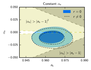
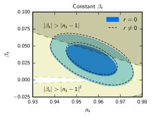
Figure 1: Constraints from Planck 2015 TT+lowTEB [1] and BICEP-Keck [22] on a constant $\alpha_{s}$ (left) and a constant $\beta_{s}$ (marginalized over $\alpha_{s}$ at the pivot scale; right), both against $n_{s}$ at the pivot scale. Dashed black contours assume a null tensor-to-scalar ratio, $r$, whereas blue contours marginalize over it. The light shaded region corresponds to the part of the parameter space where the quantity in the vertical axis becomes greater than $\left|n_{s}-1\right|^{2}$ and the dark shaded region is where it becomes greater than $\left|n_{s}-1\right|$. The naive expectation is that the true value of $\alpha_{s}$ (left) should be close to the boundary of the unshaded region and far away from the dark shaded region, whereas that of $\beta_{s}$ (right) should be well inside the unshaded region. Current constraints allow a much greater area of the parameter space.

A few ways to approach modelling a more general slow-roll scenario are available in the literature [12, 14, 23, 16, 15, 24, 25, 26, 27, 28]. In this work, we use the results from Ref. [16] (which in turn use the results from Ref. [14]), which we briefly review.

To solve for the power spectrum (Eq. (2.15)) we need to solve for the modes $y$. The second-order linear differential equation in Eq. (2.12) can be solved for $y$ using Green’s functions, with solution satisfying the boundary conditions of Eq. (2.9) given implicitly by

$$y\left(x\right)=y_{0}\left(x\right)+\frac{i}{2}\intop_{x}^{\infty}\frac{du}{u^{2}}g\left(\ln u\right)\left[y_{0}^{*}\left(u\right)y_{0}\left(x\right)-y_{0}^{*}\left(x\right)y_{0}\left(u\right)\right]y\left(u\right).$$ (2.23)

This can be solved iteratively for $y$ to successively higher order in $g$ (assuming $\left|g\right|<1$) by substituting the previous order result into the right-hand side of Eq. (2.23) (starting with $y\left(u\right)=y_{0}\left(u\right))$. The result for the power spectrum at the desired order can then be obtained by substituting into Eq. (2.15) and simplifying as much as possible. The result for the scalar power spectrum correct to quadratic order in $g$ is then [14]

$$\ln\mathcal{P}\left(\ln k\right)=\intop_{0}^{\infty}\frac{d\xi}{\xi}\left[-k\xi W^{\prime}\left(k\xi\right)\right]\left[\ln\frac{1}{f\left(\ln\xi\right)^{2}}+\frac{2}{3}\frac{f^{\prime}\left(\ln\xi\right)}{f\left(\ln\xi\right)}\right]+\frac{\pi^{2}}{2}\left[\intop_{0}^{\infty}\frac{d\xi}{\xi}m\left(k\xi\right)\frac{f^{\prime}\left(\ln\xi\right)}{f\left(\ln\xi\right)}\right]^{2}\\ -2\pi\intop_{0}^{\infty}\frac{d\xi}{\xi}m\left(k\xi\right)\frac{f^{\prime}\left(\ln\xi\right)}{f\left(\ln\xi\right)}\intop_{\xi}^{\infty}\frac{d\zeta}{\zeta}\frac{1}{k\zeta}\frac{f^{\prime}\left(\ln\zeta\right)}{f\left(\ln\zeta\right)}+{\cal{O}}\left(g^{3}\right),$$ (2.24)

where $W$ and $m$ are window functions defined by

$$W\left(x\right)=\frac{3\sin\left(2x\right)}{x^{3}}-\frac{3\cos\left(2x\right)}{x^{2}}-\frac{3\sin\left(2x\right)}{2x}-1$$ (2.25)

and

$$m\left(x\right)=\frac{2}{\pi}\left[\frac{1}{x}-\frac{\cos\left(2x\right)}{x}-\sin\left(2x\right)\right].$$ (2.26)

In this paper we are interested in relating properties of the observable power spectrum to those of the inflationary model, so we need the inverse version of this result, which can be shown to be [16]

$$\ln\frac{1}{f\left(\ln\xi\right)^{2}}=\intop_{0}^{\infty}\frac{dk}{k}m\left(k\xi\right)\ln\mathcal{P}\left(\ln k\right)-\frac{\pi^{2}}{8}\intop_{0}^{\infty}\frac{dk}{k}m\left(k\xi\right)\left[\intop_{0}^{\infty}\frac{dl}{l}\frac{\mathcal{P}^{\prime}(\ln l)}{\mathcal{P}(\ln l)}\intop_{0}^{\infty}\frac{d\zeta}{\zeta}m\left(k\zeta\right)m\left(l\zeta\right)\right]^{2}\\ +\frac{\pi}{2}\intop_{0}^{\infty}\frac{dl}{l}\frac{\mathcal{P}^{\prime}(\ln l)}{\mathcal{P}(\ln l)}\intop_{0}^{\infty}\frac{dq}{q}\frac{\mathcal{P}^{\prime}(\ln q)}{\mathcal{P}(\ln q)}\intop_{0}^{\infty}\frac{d\zeta}{\zeta}m\left(l\zeta\right)\intop_{0}^{\infty}\frac{dk}{k^{2}}m\left(k\xi\right)m\left(k\zeta\right)\intop_{\zeta}^{\infty}\frac{d\chi}{\chi^{2}}m\left(q\chi\right).$$ (2.27)

3 Exploring the limits of slow-roll

3.1 How slow is slow-roll?

To assess how much running there can be in slow-roll inflation, we would like some objective criteria to decide whether any given inflationary model is slow-roll or not. The “$\ll$” signs in Eqs. (2.3)-(2.4) defining the slow-roll approximations do not allow a clear distinction unless the numbers being compared are orders of magnitude apart. To make matters worse, Eq. (2.4) has been defined in the literature in terms of a number of slightly different slow-roll parameters (usually referred to as $\eta$), all of which would lead to different classifications of borderline cases even if we were to decide on an objective meaning for “$\ll$” in these equations.

When faced with this sort of problem it is important not to get lost in an overly semantic discussion. One pragmatic reason to care about whether a model falls under the category of slow-roll is simply to know whether the power spectrum can be straightforwardly computed using results like Eq. (2.18) and Eq. (2.24). Therefore, from the perspective of this work, the best way to define slow-roll is in terms of a quantity that can quantify how precise this formula actually is. From the derivation, the most natural quantity appears to be the parameter $g$. Unfortunately, this will result in a slightly stronger definition than using just the slow-roll approximation, as it discards scenarios in which $\delta_{2}$ is large but $\epsilon$ and $\delta_{1}$ remain small (see appendix A). Nevertheless, it is a weak enough definition that we will be able to qualitatively improve on the simplistic constraints in subsection 2.2.

Instead of committing to any arbitrary definition of what a “very small” number is, we show, for each combination of observable parameter values, how large $g$ can become during the period of time in which observable scales crossed the horizon. The reader can not only decide which values are “not small” on his/her own, but also have a good understanding of the meaning of any specific choice: the larger the allowed values, the less accurate our formulas.

3.2 Outline of the method

We start by parameterizing the observed scalar power spectrum as

$$\ln\mathcal{P}\left(\ln k\right)=\sum_{n=0}^{N}\frac{\beta_{n}}{n!}\left(\ln\frac{k}{k_{0}}\right)^{n},$$ (3.1)

where $k_{0}$ is a pivot scale and the $\beta_{n}$ coefficients are to be constrained by observations. Of course,

$$\begin{split}&\beta_{0}\equiv\ln\mathcal{P}_{0}\\ &\beta_{1}\equiv n_{s}-1\\ &\beta_{2}\equiv\alpha_{s}\\ &\beta_{3}\equiv\beta_{s}\end{split}$$ (3.2)

where $\mathcal{P}_{0}$ is the magnitude of the power spectrum at the pivot scale. For the purposes of this work, we will be interested in the cases with $N=2$ and $N=3$, for which $\beta_{N}$ have already been constrained by the Planck collaboration [1]. A natural extension of our calculations is sufficient to deal with cases with higher $N$ should observational constraints on higher-order runnings become available (it has been claimed such constraints could come from minihalo effects on 21cm fluctuations [9]). Likewise, radically different parameterizations of the power spectrum can be incorporated by making the appropriate changes to Eq. (3.1).

For each point in the $\left(\beta_{0},\beta_{1},...,\beta_{N}\right)$ parameter space, we want to know to what extent a canonical single-field inflation model must violate slow-roll during the interval of time during which observable scales left the horizon (i.e., how large its respective $g$ function must become during that time).

We proceed by defining a $g\left(\ln x\right)$ for every $k$ by inserting the power spectrum from Eq. (3.1) into Eq. (2.27), and then the resulting $f\left(\ln\xi\right)$ into Eq. (2.14). The main obstacle in the way of this calculation is the computation of the integrals in Eq. (2.27) when the power spectrum is a polynomial in $\ln\frac{k}{k_{0}}$, as we assume (in Eq. (3.1)). To solve these integrals for power spectra with non-null $\beta_{s}$, we extended known results for the standard hierarchy in the slow-roll approximation [16] (see appendix B). The results are polynomials in $\ln\left(k_{0}\xi\right)$, so $g$ can then be found straightforwardly from Eq. (2.14) by differentiation.

Once these $g$ functions have been found for $k$ corresponding to observable scales, we check the absolute value of $g$ at $x=1+\epsilon=1+\frac{r}{16}$, corresponding to the time of horizon-crossing to leading order in $\epsilon$ (see, e.g., Eqs. (A.2) and (A.9) in appendix A).

4 Results

The method described in section 3 was implemented in a Python code using the results from appendix B. This allowed us to draw contour plots indicating how large $g$ can get during the relevant epochs for different pivot values of $n_{s}$, $\alpha_{s}$, and $\beta_{s}$, assuming that Eq. (3.1) holds for a specific range of observable scales. In this work we present results for three different ranges of observable scales, from $k_{\rm min}=10^{-3}\mathrm{Mpc^{-1}}$ (set by the largest scales that can be reasonably well measured) up to: $k_{\rm max}=0.3\mathrm{Mpc^{-1}}$ (spanning about 6 efoldings), roughly corresponding to the smallest scale well constrained by Planck; $k_{\rm max}=100\mathrm{Mpc^{-1}}$ (spanning about 12 efoldings), roughly corresponding to a future constraint from 21cm observations [29, 9]; and $k_{\rm max}=10^{4}\mathrm{Mpc^{-1}}$ (spanning about 16 efoldings), roughly corresponding to the smallest scale constrained by spectral distortions [30]. The pivot scale is taken to be $k_{0}=0.05\mathrm{Mpc^{-1}}$, the Planck pivot scale.

In order to make statements about the status of this class of canonical single-field slow-roll inflation, we use CosmoMC [32, 33] to superimpose current constraints from Planck 2015 data (temperature plus low-$\ell$ polarization, TT + lowTEB [1]) and the latest BICEP-KECK-Planck joint analysis [22], showing the $1\sigma$ and $2\sigma$ allowed regions. Additionally, we plot contours for the inferred maximum values of $g$ from current observations against $\alpha_{s}$ and $\beta_{s}$.

4.1 Constant running ($N=2$)

If we limit ourselves to the case with constant $\alpha_{s}$ (corresponding to $N=2$ in Eq. (3.1)) we have only two relevant observables: $\alpha_{s}$ and $n_{s}$ at the pivot scale. The corresponding plots for the magnitude of $g$ can be found in figure 2.

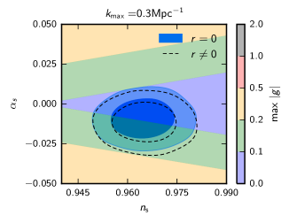
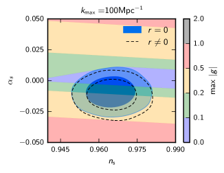
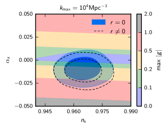
Figure 2: Slow-roll and observational constraints on parameterizations of the power spectrum with a constant $\alpha_{s}$. The observational contours are Planck 2015 TT+lowTEB and joint BICEP-Keck-Planck constraints for a constant $\alpha_{s}$ and $n_{s}$ at the pivot scale. Dashed black contours assume a null tensor-to-scalar ratio, $r$, whereas blue contours marginalise over allowed values of $r\geq 0$. The coloured areas indicate the maximum magnitude of $g$ during the interval of time during which constrained scales left the horizon. Note that for $g>1$ our method breaks down as Eq. (2.24) ceases to be valid.

For the currently constrained range of scales even the 2$\sigma$ observational contours never go beyond the $\left|g\right|<0.2$ line (which is still comfortably much less than unity). Even our futuristic scenario with $k_{\rm max}=100\rm{Mpc^{-1}}$ has the 2$\sigma$ contour being well inside the $\left|g\right|<0.5$ region (which corresponds to a borderline case for which the designation of “slow-roll” is rather dubious, but which still does not allow us to make a very strong statement). Only a futuristic scenario with $k_{\rm max}=10^{4}\rm{Mpc^{-1}}$ would permit a measurement of constant $\alpha_{s}$ to provide a strong test of slow roll. However, constraints from spectral distortions would depend on integrals of the power spectrum over the range $1{\rm Mpc}^{-1}\lesssim k\lesssim 10^{4}{\rm Mpc}^{-1}$, and cannot on their own establish the constancy of $\alpha_{s}$ (even if they could accurately measure $\alpha_{s}$ provided it is assumed to be constant [30]).

These conclusions are confirmed (and more easily seen) in the plots in figure 3, which show the bounds on the maximum magnitude of $g$ inferred from the bounds on the running and the spectral index. Note that their asymmetric boomerang shape is due to the modulus sign in $\left|g\right|$ as well as the significant deviation of the Planck best-fit value for $\alpha_{s}$ from zero.

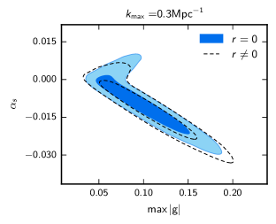
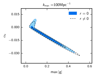
Figure 3: Bounds, over the constrained ranges of scales, on the maximum magnitude of $g$ inferred from Planck 2015 TT+lowTEB and joint BICEP-Keck-Planck constraints on a constant $\alpha_{s}$ marginalized over $n_{s}$ at the pivot scale. Filled contours assume $r=0$ whereas solid lines marginalize over allowed values of $r\geq 0$.

4.2 Constant running of the running ($N=3$)

If we allow the running to vary with a constant $\beta_{s}$ (corresponding to $N=3$ in Eq. (3.1)) we have three relevant observables: the constant $\beta_{s}$, as well as the values of $\alpha_{s}$ and $n_{s}$ at the pivot scale. In order to illustrate typical constraints, we present the plots corresponding to $\beta_{s}=0.029$ (the Planck best fit) in figure 4 (higher values of $\beta_{s}$ would result in a more dramatic version of these plots, whereas lower values would yield plots more similar to those in figure 2).

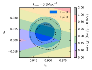
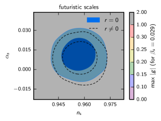
Figure 4: Slow-roll and observational constraints on parameterizations of the power spectrum with a constant $\beta_{s}=0.029$. The observational contours are Planck 2015 TT+lowTEB and joint BICEP-Keck-Planck constraints for $\alpha_{s}$ and $n_{s}$ at the pivot scale. Dashed black contours assume a null tensor-to-scalar ratio, $r$, whereas blue contours marginalise over allowed values of $r\geq 0$. The coloured areas indicate the maximum magnitude of $g$ during the interval of time during which the constrained scales left the horizon (“futuristic scales” denoting both $k_{\rm max}=100\rm{Mpc^{-1}}$ and $k_{\rm max}=10^{4}\rm{Mpc^{-1}}$). Note that for $g>1$ (as is the case everywhere on the plot on the right-hand side) our method breaks down as Eq. (2.24) ceases to be valid.

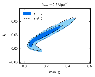
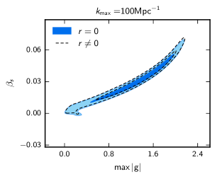
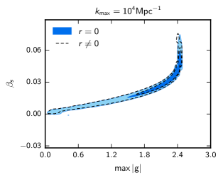
Figure 5: Bounds, over the constrained ranges of scales, on the maximum magnitude of $g$ inferred from Planck 2015 TT+lowTEB and BICEP-Keck constraints on a constant $\beta_{s}$ marginalized over $\alpha_{s}$ and $n_{s}$ at the pivot scale. Filled contours assume $r=0$ whereas solid lines marginalize over allowed values of $r\geq 0$. Note that for $g>1$ our method breaks down as Eq. (2.24) ceases to be valid.

To comment more generally on whether this class of slow-roll models can be ruled out by measuring $\beta_{s}$ over the range of its currently allowed possible values, it is easier to focus on the constraints on the maximum magnitude of $g$ shown in figure 5 (since they conveniently reduce the relevant three-dimensional information to simple two-dimensional contours). The current preference for $\beta_{s}\neq 0$ is driven by large scales, but small-scale data is consistent with constant spectral index, so as more small-scale data is added it is plausible that constraints on $\beta_{s}$ will converge to be closer to zero in the future. However, if they do not, it is quite possible that a future detection of non-zero running of the running could significantly disfavour this class of single-field slow-roll inflation, but only if information on a slightly wider range of scales is obtained (about an extra efolding should suffice for large values of $\beta_{s}$ to clearly lead to high values of $\left|g\right|$, given how some are already at the borderline $\left|g\right|\sim 0.5$.). In particular, a future detection near Planck’s current best fit ($\beta_{s}=0.029$) could clearly rule out this class of slow roll.

That the larger values of constant $\beta_{s}$ would rule out simple slow-roll inflation models should not be a surprise. An intuitive argument for this uses the fact that, under fairly general assumptions, to leading order in slow roll, $n_{s}-1$ can be written in a simpler form as a sum of small $\delta_{n}$ parameters (of which Eq. (2.19) is the first-order truncation) [12]. If $\beta_{s}=\mathcal{O}(0.05)$ and constant, $n_{s}$ would change by $\mathcal{O}(1)$ over the observable range of scales, implying that this form of $n_{s}-1$ cannot be valid everywhere.

4.3 Consequences for the power spectrum

It is interesting to consider what current data say about the allowed range for the small-scale power spectrum that could be observed by future data. Assuming that the parameterization we have used (with constant $\beta_{s}$) can be extended, current Planck constraints with non-zero $\beta_{s}$ allow the power spectrum to grow to order unity at the smallest scales we consider (which would already be ruled out by other probes [30, 34]). Therefore, it is instructive to see how the requirement of slow roll (as defined by a maximum allowed magnitude of $g$ over constrained scales) would affect this extrapolation, and how that compares with the effect of the naive expectations resulting from the imposition of the usual hierarchy on slow-roll parameters.

Our inferred constraints on the power spectrum are shown in figure 6: the assumption of slow roll leads to significantly tilted and narrower bounds on the small-scale power spectrum (compared to assuming only Planck constraints), especially for the case of constant $\beta_{s}$.

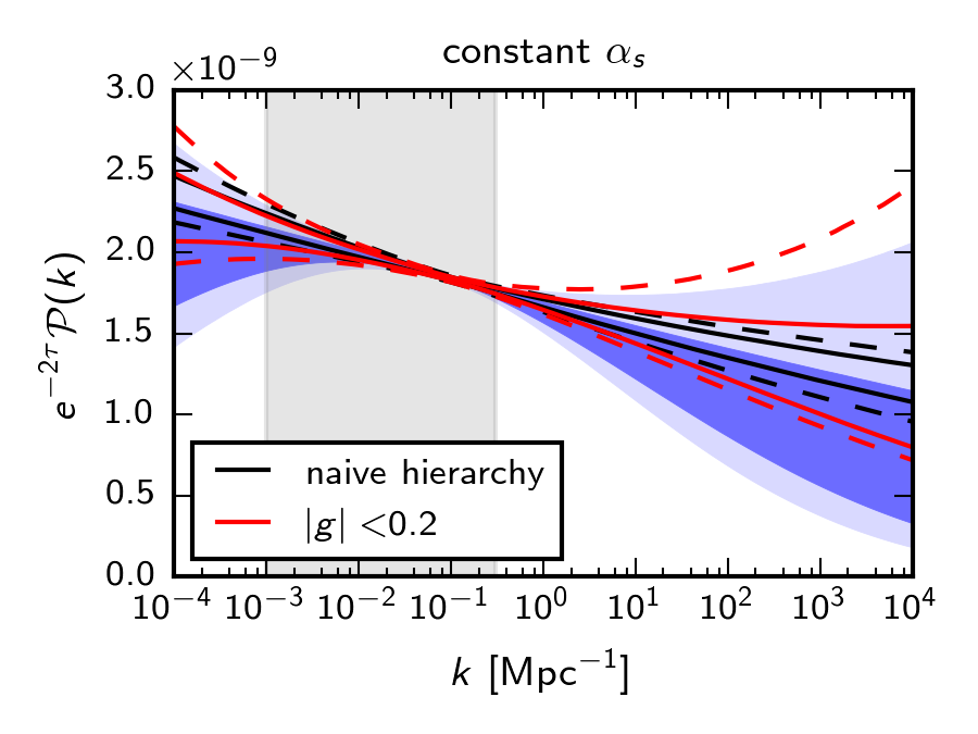
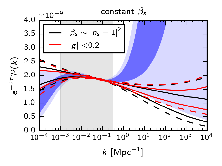
Figure 6: Consequences of the imposition of slow roll (defined by the smallness of $g$) for the power spectrum scaled by $e^{-2\tau}$, where $\tau$ is the optical depth (whose value affects the amplitude of the spectrum, but not its shape). The blue contours represent the 68% (dark blue) and 95% (light blue) limits on the allowed values of the power spectrum (rescaled by a factor of $e^{-2\tau}$) extrapolated from Planck 2015 TT+lowTEB constraints (over gray shaded scales) assuming a constant $\alpha_{s}$ (left) and a constant $\beta_{s}$ (right), for different values of $k$. The solid and dashed red contours represent the 68% and 95% limits on the fraction of these spectra for which $\left|g\right|<0.2$ for the range of scales corresponding to $10^{-3}\rm{Mpc^{-1}}<k<10^{4}\rm{Mpc^{-1}}$. The solid and dashed black contours represent the 68% and 95% limits on the fraction of these spectra corresponding to the unshaded regions in figure 1 (note that for the plot on the right the limits of this region already violate the naive expectation for the magnitude of $\beta_{s}$).

5 Conclusions

We devised a straightforward method to assess whether specific observed values of the running (of the running) of the spectral index are consistent with canonical single-field slow-roll inflation. We showed that slow roll is much harder to discard than simple expectations based on a hierarchy of slow-roll parameters suggest, and in particular that for constant running any of the currently allowed values would not necessarily imply a violation of slow roll over observable scales. However, a detection of constant $\beta_{s}$ significantly away from zero could be much more powerful: a firmer detection over currently-available scales could be enough to restrict slow-roll inflation to a region of borderline validity, and future data over a wider range of scales could invalidate slow roll for the simple parameterization of the power spectrum assumed.

There are, however, a couple of limitations of our approach:

- Firstly, we redefined slow-roll as meaning $\left|g\right|\ll 1$, which, despite not assuming any hierarchy of slow-roll parameters, is a somewhat stronger condition than the general definition of $\epsilon,\left|\delta_{1}\right|\ll 1$ (see the conclusions of appendix A). Nevertheless, this still corresponds to a very simple and wide class of models, including all the ones which make the wider class so popular (slow-roll formulae for the power spectrum should break down for the models left out).

- Secondly, we follow a constructive approach: for each specific combination of observable parameters $\{n_{s},\alpha_{s},\beta_{s},...\}$ we find a function $g\left(\ln\xi\right)$ which generates them and check whether it breaks our weaker definition of slow-roll during the time during which observably measurable scales crossed the horizon. Inevitably, we can only find (or fail to find) examples of models which generate power spectra of the specific kind assumed (in the case of this work, with constant $\alpha_{s}$ or $\beta_{s}$). In the case of constant $\alpha_{s}$, an existence proof is sufficient to demonstrate that models do not violate slow roll. However, in cases where slow-roll is violated, our assumption is restrictive and different parameterizations (e.g., involving oscillatory features, or large-scale features) might lead to different conclusions. It would be straightforward to generalize our method to constrain both higher-order runnings and completely different parameterizations by making appropriate changes to Eq. (3.1).

Due to its smallness, the tensor-to-scalar ratio does not noticeably affect our results.

6 Acknowledgements

We thank Ewan Stewart and Daniel Passos for helpful comments.

JV is supported by an STFC studentship, CB is supported by a Royal Society University Research Fellowship, and AL acknowledges support from the European Research Council under the European Union’s Seventh Framework Programme (FP/2007-2013) / ERC Grant Agreement No. [616170] and from the Science and Technology Facilities Council [grant number ST/L000652/1].

Appendix A $g$ and the slow-roll parameters

In this work, slow-roll is tested via the $g$ function defined in Eq. (2.14) rather than directly via the slow-roll parameters. We relate the two here.

A.1 Slow-roll parameters from conformal time

The main difficulty in relating $g$ to the slow-roll parameters stems from the terms in $g$ which are related to the conformal time. We thus start by manipulating the usual expression for (minus) the conformal time,

$$\xi\left(t\right)=\intop_{t}^{\infty}\frac{dt^{{}^{\prime}}}{a\left(t^{{}^{\prime}}\right)}=\intop_{a\left(t\right)}^{\infty}\frac{da}{Ha^{2}}=\frac{1}{a\left(t\right)H\left(t\right)}-\intop_{a\left(t\right)}^{\infty}\frac{\dot{H}}{H^{2}}\frac{da}{a\dot{a}}=\frac{1}{a\left(t\right)H\left(t\right)}-\intop_{a\left(t\right)}^{\infty}\frac{\dot{H}}{H^{2}}\frac{da}{a^{2}H}.$$ (A.1)

Using Eq. (2.3), we write it as

$$\xi=\frac{1}{aH}\left[1+\bar{\epsilon}\right],$$ (A.2)

where $\bar{\epsilon}$ is given by

$$\bar{\epsilon}\left(\xi\right)\equiv a\left(\xi\right)H\left(\xi\right)\intop_{0}^{\xi}\epsilon(\tilde{\xi})d\tilde{\xi}=\frac{1}{\left\langle\epsilon\right\rangle_{\xi}^{-1}-1},$$ (A.3)

$\left\langle\epsilon\right\rangle$ being the conformal time average of $\epsilon$ at a given instant, defined as

$$\left\langle\epsilon\right\rangle_{\xi}\equiv\frac{1}{\xi}\intop_{0}^{\xi}\epsilon(\tilde{\xi})d\tilde{\xi.}$$ (A.4)

From Eq. (2.3), it can be easily seen that

$$\frac{d\epsilon}{d\ln\xi}=-\left(1+\bar{\epsilon}\right)\left(2\epsilon^{2}+2\epsilon\delta_{1}\right),$$ (A.5)

so variations in $\epsilon$ are second-order in slow roll and thus $\left\langle\epsilon\right\rangle$ and $\bar{\epsilon}$ are not expected to differ from $\epsilon$ at first order.

In fact, if we further assume that $\epsilon$ is well-behaved (in the sense that it can be expressed as a Taylor series in the domain of integration of Eq. (A.4)), we can write $\left\langle\epsilon\right\rangle$ as

$$\left\langle\epsilon\right\rangle_{\xi}=\epsilon+\sum_{n=1}^{\infty}\frac{d^{n}\epsilon}{d\xi^{n}}\frac{\left(-\xi\right)^{n}}{\left(n+1\right)!}=\epsilon+\sum_{n=1}^{\infty}\left(-aH\right)^{-n}\frac{d^{n}\epsilon}{d\xi^{n}}\frac{\left(1+\bar{\epsilon}\right)^{n}}{\left(n+1\right)!}.$$ (A.6)

Combining this with Eq. (A.5) and its equivalent for $\delta_{n}$,

$$\frac{d\delta_{n}}{d\ln\xi}=-\left(1+\bar{\epsilon}\right)\left(\delta_{n+1}+n\epsilon\delta_{n}-n\delta_{1}\delta_{n}\right),$$ (A.7)

it can be seen that, to second order in the slow-roll parameters,

$$\left\langle\epsilon\right\rangle_{\xi}\approx\epsilon+2\left(\epsilon+\sum_{p=1}^{\infty}\delta_{p}\right)\epsilon$$ (A.8)

(the right-hand side being evaluated at minus conformal time $\xi$) and

$$\bar{\epsilon}\approx\epsilon\left(1+3\epsilon+2\sum_{p=1}^{\infty}\delta_{p}\right).$$ (A.9)

A.2 $g$ from $f$

Using these results, the $f$ function defined in Eq. (2.13) can be written as

$$f\left(\ln x\right)=2\pi\frac{\dot{\phi}}{H^{2}}\left[1+\bar{\epsilon}\right].$$ (A.10)

Now, using

$$\frac{d\ln\dot{\phi}}{d\ln\xi}=-\left(1+\bar{\epsilon}\right)\delta_{1},$$ (A.11)

$$\frac{d\ln H}{d\ln\xi}=\left(1+\bar{\epsilon}\right)\epsilon,$$ (A.12)

and

$$\frac{d\bar{\epsilon}}{d\ln\xi}=\left(1+\bar{\epsilon}\right)\left(\epsilon-\bar{\epsilon}+\epsilon\bar{\epsilon}\right),$$ (A.13)

we can find

$$\frac{d\ln f}{d\ln\xi}=-\bar{\epsilon}-\epsilon-\delta_{1}-\bar{\epsilon}\epsilon-\bar{\epsilon}\delta_{1}.$$ (A.14)

In addition, using also Eqs. (A.5) and (A.7), we can find

$$\frac{d^{2}\ln f}{d\ln\xi^{2}}=\left(1+\bar{\epsilon}\right)\left(\bar{\epsilon}-\epsilon+\delta_{2}+\bar{\epsilon}\delta_{1}+\bar{\epsilon}\delta_{2}+\epsilon^{2}+2\epsilon\delta_{1}-\delta_{1}^{2}+\bar{\epsilon}\epsilon^{2}-\bar{\epsilon}\delta_{1}^{2}\right).$$ (A.15)

Finally, using the definition of $g$ (Eq. (2.14)), we have

$$g\left(\ln x\right)=\left[4\bar{\epsilon}+2\epsilon+3\delta_{1}+\delta_{2}+2\bar{\epsilon}^{2}+4\bar{\epsilon}\epsilon+5\bar{\epsilon}\delta_{1}+2\bar{\epsilon}\delta_{2}+2\epsilon^{2}+4\epsilon\delta_{1}+2\bar{\epsilon}^{2}\epsilon+2\bar{\epsilon}^{2}\delta_{1}\right.\\ \left.+\bar{\epsilon}^{2}\delta_{2}+4\bar{\epsilon}\epsilon^{2}+6\bar{\epsilon}\epsilon\delta_{1}+\bar{\epsilon}\delta_{1}^{2}+2\bar{\epsilon}^{2}\epsilon^{2}+2\bar{\epsilon}^{2}\epsilon\delta_{1}+\bar{\epsilon}^{2}\delta_{1}^{2}\right]_{\xi=\frac{x}{k}}.$$ (A.16)

Appendix B Evaluating the integrals

We shall see how each of the integrals in Eq. (2.27) can be calculated in a straightforward (albeit tedious) manner when assuming Eq. (3.1).

B.1 $\mathcal{I}_{1}(\xi)\equiv\intop_{0}^{\infty}\frac{dk}{k}m\left(k\xi\right)\ln\mathcal{P}\left(\ln k\right)$

Assuming Eq. (3.1), this term can be rewritten as

$$\mathcal{I}_{1}(\xi)=\sum_{n=0}^{N}\frac{\beta_{n}}{n!}\intop_{0}^{\infty}\frac{dk}{k}m\left(k\xi\right)\left(\ln\frac{k}{k_{0}}\right)^{n}\equiv\sum_{n=0}^{N}\frac{\beta_{n}}{n!}I_{n}\left(k_{0}\xi\right),$$ (B.1)

where we have defined

$$I_{n}\left(y\right)\equiv\intop_{0}^{\infty}\frac{dx}{x}m\left(x\right)\left(\ln\frac{x}{y}\right)^{n}=\sum_{k=0}^{n}\left(\begin{array}[]{c}n\\ k\end{array}\right)I_{n-k}\left(1\right)\left(-\ln y\right)^{k}=\sum_{k=0}^{n}\left(\begin{array}[]{c}n\\ k\end{array}\right)I_{k}\left(1\right)\left(-\ln y\right)^{n-k}.$$ (B.2)

One way of iteratively computing the constant terms $I_{k}\left(1\right)$ is by considering the more general family of integrals,

$$\tilde{I}_{k}\left(\alpha\right)\equiv\intop_{0}^{\infty}\frac{dx}{x}m\left(x\right)\left(\ln x\right)^{k}x^{\alpha},$$ (B.3)

which are related to the terms we want to compute by

$$\tilde{I}_{k}\left(0\right)=I_{k}\left(1\right).$$ (B.4)

The $\tilde{I}_{k}$ obey the recursive formula

$$\frac{\partial\tilde{I}_{k}\left(\alpha\right)}{\partial\alpha}=\tilde{I}_{k+1}\left(\alpha\right),$$ (B.5)

which gives us a simple way to generate all the integrals we are interested in (since we are not interested in non-integer $n$). The recursion can start from $\tilde{I}_{0}$, which can be shown to be the continuous version of

$$\tilde{I}_{0}\left(\alpha\right)=-\frac{2^{1-\alpha}}{\pi}\left(1+\alpha\right)\Gamma\left(\alpha-1\right)\sin\left(\frac{\pi}{2}\alpha\right).$$ (B.6)

Putting all of this together, we can finally write the relevant integrals up to $N=3$ as

$$I_{0}\left(k_{0}\xi\right)=1$$ (B.7)

$$I_{1}\left(k_{0}\xi\right)=-\ln\left(k_{0}\xi\right)-\gamma+2-\ln 2$$ (B.8)

$$I_{2}\left(k_{0}\xi\right)=\ln^{2}\left(k_{0}\xi\right)+\left(-4+2\gamma+2\ln 2\right)\ln\left(k_{0}\xi\right)+\frac{\pi^{2}}{12}+\gamma\left(-4+\gamma+2\ln 2\right)+\left(\ln 2-2\right)^{2}$$ (B.9)

$$I_{3}\left(k_{0}\xi\right)=-\ln^{3}\left(k_{0}\xi\right)+3\left(2-\gamma-\ln 2\right)\ln^{2}\left(k_{0}\xi\right)\\ -\frac{1}{4}\left(12\left(\gamma-2\right)^{2}+\pi^{2}+12\ln 2\left(-4+2\gamma+\ln 2\right)\right)\ln\left(k_{0}\xi\right)\\ +\frac{1}{4}\left(48+2\pi^{2}-8\zeta\left(3\right)-\gamma\left(48+4\left(\gamma-6\right)\gamma+\pi^{2}\right)\right.\\ \left.-4\ln^{3}2+24\ln^{2}2-12\gamma\ln^{2}2-\left(12\left(\gamma-2\right)^{2}+\pi^{2}\right)\ln 2\right),$$ (B.10)

where $\gamma\simeq 0.5772$ is the Euler-Mascheroni constant and $\zeta$ is the Riemann zeta function, the next integral (which it turns out will be relevant further ahead) being given by

$$I_{4}\left(k_{0}\xi\right)=\ln^{4}\left(k_{0}\xi\right)+4\left(-2+\gamma+\ln 2\right)\ln^{3}\left(k_{0}\xi\right)\\ +\frac{1}{2}\left(12\gamma^{2}+\pi^{2}+24\gamma\left(\ln 2-2\right)+12\left(\ln 2-2\right)^{2}\right)\ln^{2}\left(k_{0}\xi\right)\\ +\left(8\zeta\left(3\right)-48+4\ln^{3}2-24\ln^{2}2+48\ln 2+4\gamma^{3}\right.\\ \left.+\gamma\left(\pi^{2}+12\left(\ln 2-2\right)^{2}\right)+12\gamma^{2}\left(\ln 2-2\right)+\pi^{2}\left(\ln 2-2\right)\right)\times\ln\left(k_{0}\xi\right)\\ -16\zeta\left(3\right)+\gamma\left(4\left(2\zeta\left(3\right)-12+\ln^{3}2-6\ln^{2}2+12\ln 2\right)+\pi^{2}\left(\ln 2-2\right)\right)\\ +8\zeta\left(3\right)\ln 2+\frac{19\pi^{4}}{240}+2\pi^{2}+\gamma^{4}+48+\ln^{4}2-8\ln^{3}2\\ +\frac{1}{2}\pi^{2}\ln^{2}2+24\ln^{2}2-2\pi^{2}\ln 2-48\ln 2+4\gamma^{3}\left(\ln 2-2\right)+\frac{1}{2}\gamma^{2}\left(\pi^{2}+12\left(\ln 2-2\right)^{2}\right).$$ (B.11)

B.2 $\mathcal{I}_{2}(\xi)\equiv-\frac{\pi^{2}}{8}\intop_{0}^{\infty}\frac{dk}{k}m\left(k\xi\right)\left[\intop_{0}^{\infty}\frac{dl}{l}\frac{\mathcal{P}^{\prime}(\ln l)}{\mathcal{P}(\ln l)}\intop_{0}^{\infty}\frac{d\zeta}{\zeta}m\left(k\zeta\right)m\left(l\zeta\right)\right]^{2}$

Assuming Eq. (3.1), this term can be written as

$$\mathcal{I}_{2}(\xi)=-\frac{\pi^{2}}{8}\intop_{0}^{\infty}\frac{dk}{k}m\left(k\xi\right)\left[\sum_{n=0}^{N-1}\frac{\beta_{n+1}}{n!}\intop_{0}^{\infty}\frac{dl}{l}\intop_{0}^{\infty}\frac{d\zeta}{\zeta}m\left(k\zeta\right)m\left(l\zeta\right)\left(\ln\frac{l}{k_{0}}\right)^{n}\right]^{2}.$$ (B.12)

It is convenient to focus first on the integral being squared, which we can write as a sum of terms of the form

$$\intop_{0}^{\infty}\frac{dl}{l}\intop_{0}^{\infty}\frac{d\zeta}{\zeta}m\left(k\zeta\right)m\left(l\zeta\right)\left(\ln\frac{l}{k_{0}}\right)^{n}=\intop_{0}^{\infty}\frac{d\zeta}{\zeta}m\left(k\zeta\right)I_{n}\left(k_{0}\zeta\right),$$ (B.13)

where we changed the order of integration and used the definition of $I_{n}$ from Eq. (B.2). Given that these functions can be quite messy in appearance, but are always polynomials in $\ln\left(k_{0}\xi\right)$, we write them as

$$I_{n}\left(k_{0}\xi\right)\equiv\sum_{i=0}^{n}c_{n}\left[i\right]\ln^{i}\left(k_{0}\xi\right),$$ (B.14)

where the $c_{n}\left[i\right]$ coefficients can be found as described in subsection B.1 (the relevant ones being trivially obtained by comparison with Eqs. (B.7), (B.8), (B.9), (B.10), and (B.11)). This “inner” integral thus becomes

$$\intop_{0}^{\infty}\frac{d\zeta}{\zeta}m\left(k\zeta\right)I_{n}\left(k_{0}\zeta\right)=\sum_{i=0}^{n}c_{n}\left[i\right]\intop_{0}^{\infty}\frac{d\zeta}{\zeta}m\left(k\zeta\right)\ln^{i}\left(k_{0}\zeta\right)=\sum_{i=0}^{n}\sum_{j=0}^{i}c_{n}\left[i\right]c_{i}\left[j\right]\left(\ln\frac{k}{k_{0}}\right)^{j}.$$ (B.15)

Substituting this into Eq. (B.12) and changing the order of summation we are left with

$$\sum_{n=0}^{N-1}\frac{\beta_{n+1}}{n!}\intop_{0}^{\infty}\frac{dl}{l}\intop_{0}^{\infty}\frac{d\zeta}{\zeta}m\left(k\zeta\right)m\left(l\zeta\right)\left(\ln\frac{l}{k_{0}}\right)^{n}=\sum_{j=0}^{N-1}\tilde{c}_{N}\left[j\right]\left(\ln\frac{k}{k_{0}}\right)^{j},$$ (B.16)

where we have defined

$$\tilde{c}_{N}\left[j\right]\equiv\sum_{n=j}^{N-1}\sum_{i=j}^{n}\frac{\beta_{n+1}}{n!}c_{n}\left[i\right]c_{i}\left[j\right].$$ (B.17)

Finally, we can tackle the full double integral, writing

$$\mathcal{I}_{2}(\xi)=-\frac{\pi^{2}}{8}\sum_{i=0}^{N-1}\sum_{j=0}^{N-1}\tilde{c}_{N}\left[i\right]\tilde{c}_{N}\left[j\right]\intop_{0}^{\infty}\frac{dk}{k}m\left(k\xi\right)\left(\ln\frac{k}{k_{0}}\right)^{i+j}$$ (B.18)

which, using Eq. (B.14) once more, simplifies to

$$\mathcal{I}_{2}(\xi)=-\frac{\pi^{2}}{8}\sum_{i=0}^{N-1}\sum_{j=0}^{N-1}\sum_{s=0}^{i+j}\tilde{c}_{N}\left[i\right]\tilde{c}_{N}\left[j\right]c_{i+j}\left[s\right]\ln^{s}\left(k_{0}\xi\right).$$ (B.19)

Here, we finally see why Eq. (B.11) was needed (since $s$ can vary up to $s=4$ for $N=3$).

B.3 $\mathcal{I}_{3}(\xi)\equiv\frac{\pi}{2}\intop_{0}^{\infty}\frac{dl}{l}\frac{\mathcal{P}^{\prime}(\ln l)}{\mathcal{P}(\ln l)}\intop_{0}^{\infty}\frac{dq}{q}\frac{\mathcal{P}^{\prime}(\ln q)}{\mathcal{P}(\ln q)}\intop_{0}^{\infty}\frac{d\zeta}{\zeta}m\left(l\zeta\right)\intop_{0}^{\infty}\frac{dk}{k^{2}}m\left(k\xi\right)m\left(k\zeta\right)\intop_{\zeta}^{\infty}\frac{d\chi}{\chi^{2}}m\left(q\chi\right)$

Assuming Eq. (3.1), this term can be written as

$$\mathcal{I}_{3}(\xi)=\frac{\pi}{2}\sum_{n=0}^{N-1}\sum_{s=0}^{N-1}\frac{\beta_{n+1}}{n!}\frac{\beta_{s+1}}{s!}\times\\ \intop_{0}^{\infty}\frac{dl}{l}\intop_{0}^{\infty}\frac{dq}{q}\intop_{0}^{\infty}\frac{d\zeta}{\zeta}m\left(l\zeta\right)\intop_{0}^{\infty}\frac{dk}{k^{2}}m\left(k\xi\right)m\left(k\zeta\right)\intop_{\zeta}^{\infty}\frac{d\chi}{\chi^{2}}m\left(q\chi\right)\left(\ln\frac{l}{k_{0}}\right)^{n}\left(\ln\frac{q}{k_{0}}\right)^{s},$$ (B.20)

which we now can solve using a similar method to the previous subsections. For example, using Eq. (B.14) and integrating with respect to $l$ and $q$ we are left with

$$\sum_{n=0}^{N-1}\sum_{s=0}^{N-1}\sum_{i=0}^{n}\sum_{j=0}^{s}\frac{\pi}{2}\frac{\beta_{n+1}}{n!}\frac{\beta_{s+1}}{s!}c_{n}\left[i\right]c_{s}\left[j\right]\intop_{0}^{\infty}\frac{d\zeta}{\zeta}\ln^{i}\left(k_{0}\zeta\right)\intop_{0}^{\infty}\frac{dk}{k^{2}}m\left(k\xi\right)m\left(k\zeta\right)\intop_{\zeta}^{\infty}\frac{d\chi}{\chi^{2}}\ln^{j}\left(k_{0}\chi\right).$$ (B.21)

Focussing on the integral with respect to $\chi$, a simple change of variables gives

$$\intop_{\zeta}^{\infty}\frac{d\chi}{\chi^{2}}\ln^{j}\left(k_{0}\chi\right)=k_{0}\intop_{k_{0}\zeta}^{\infty}\frac{dx}{x^{2}}\ln^{j}\left(x\right)=k_{0}\intop_{\ln\left(k_{0}\zeta\right)}^{\infty}t^{j}e^{-t}dt\equiv k_{0}\Gamma\left(j+1,\ln\left(k_{0}\zeta\right)\right)$$ (B.22)

where $\Gamma$ is the (upper) incomplete gamma function. Since $j$ is an integer, this can be explicitly written as the type of polynomial we are interested in by using the known relation

$$\Gamma\left(j+1,\ln\left(k_{0}\zeta\right)\right)=\frac{j!}{k_{0}\zeta}\sum_{\sigma=0}^{j}\frac{\ln^{\sigma}\left(k_{0}\zeta\right)}{\sigma!}.$$ (B.23)

The full integral thus becomes

$$\sum_{n=0}^{N-1}\sum_{s=0}^{N-1}\sum_{i=0}^{n}\sum_{j=0}^{s}\sum_{\sigma=0}^{j}\frac{\beta_{n+1}}{n!}\frac{\beta_{s+1}}{s!}\frac{\pi}{2}\frac{j!}{\sigma!}c_{n}\left[i\right]c_{s}\left[j\right]\intop_{0}^{\infty}\frac{d\zeta}{\zeta^{2}}\intop_{0}^{\infty}\frac{dk}{k^{2}}m\left(k\xi\right)m\left(k\zeta\right)\ln^{i+\sigma}\left(k_{0}\zeta\right),$$ (B.24)

which can be tackled by noticing that

$$\intop_{0}^{\infty}\frac{d\zeta}{\zeta^{2}}m\left(k\zeta\right)\ln^{i+\sigma}\left(k_{0}\zeta\right)=k\intop_{0}^{\infty}\frac{dx}{x^{2}}m\left(x\right)\ln^{i+\sigma}\left(\frac{k_{0}}{k}x\right)\\ =\sum_{\rho=0}^{i+\sigma}\binom{i+\sigma}{\rho}k\left(\ln\frac{k_{0}}{k}\right)^{\rho}\intop_{0}^{\infty}\frac{dx}{x^{2}}m\left(x\right)\left(\ln x\right)^{i+\sigma-\rho}\equiv\sum_{\rho=0}^{i+\sigma}\binom{i+\sigma}{\rho}k\left(\ln\frac{k_{0}}{k}\right)^{\rho}\tilde{I}_{i+\sigma-\rho}\left(-1\right),$$ (B.25)

where in the last step we used the definition of $\tilde{I}$ from Eq. (B.3). The full integral is therefore reduced to a sextuple sum of single integrals,

$$\sum_{n=0}^{N-1}\sum_{s=0}^{N-1}\sum_{i=0}^{n}\sum_{j=0}^{s}\sum_{\sigma=0}^{j}\sum_{\rho=0}^{i+\sigma}\frac{\beta_{n+1}}{n!}\frac{\beta_{s+1}}{s!}\frac{\pi}{2}\binom{i+\sigma}{\rho}\frac{j!}{\sigma!}\tilde{I}_{i+\sigma-\rho}\left(-1\right)c_{n}\left[i\right]c_{s}\left[j\right]\intop_{0}^{\infty}\frac{dk}{k}m\left(k\xi\right)\left(-\ln\frac{k}{k_{0}}\right)^{\rho}.$$ (B.26)

The remaining integral is simply $\left(-1\right)^{\rho}I_{\rho}\left(k_{0}\xi\right)$, allowing us to write the final result as the following septuple sum of known and given terms (keeping in mind that the method for finding out any $\tilde{I}$ was shown in subsection B.1)

$$\sum_{n=0}^{N-1}\sum_{s=0}^{N-1}\sum_{i=0}^{n}\sum_{j=0}^{s}\sum_{\sigma=0}^{j}\sum_{\rho=0}^{i+\sigma}\sum_{\delta=0}^{\rho}\frac{\beta_{n+1}}{n!}\frac{\beta_{s+1}}{s!}\frac{\pi}{2}\binom{i+\sigma}{\rho}\frac{j!}{\sigma!}\left(-1\right)^{\rho}\tilde{I}_{i+\sigma-\rho}\left(-1\right)c_{n}\left[i\right]c_{s}\left[j\right]c_{\rho}\left[\delta\right]\ln^{\delta}\left(k_{0}\xi\right),$$ (B.27)

References

- [1] Planck collaboration, P. A. R. Ade et al., Planck 2015 results. XX. Constraints on inflation, Astron. Astrophys. 594 (2016) A20, [1502.02114].
- [2] J. Martin, C. Ringeval and V. Vennin, Encyclopaedia Inflationaris, Phys. Dark Univ. 5-6 (2014) 75–235, [1303.3787].
- [3] V. Vennin, K. Koyama and D. Wands, Inflation with an extra light scalar field after Planck, JCAP 1603 (2016) 024, [1512.03403].
- [4] S. Renaux-Petel, Primordial non-Gaussianities after Planck 2015: an introductory review, Comptes Rendus Physique 16 (2015) 969–985, [1508.06740].
- [5] P. Adshead, R. Easther, J. Pritchard and A. Loeb, Inflation and the Scale Dependent Spectral Index: Prospects and Strategies, JCAP 1102 (2011) 021, [1007.3748].
- [6] K. Kohri, Y. Oyama, T. Sekiguchi and T. Takahashi, Precise Measurements of Primordial Power Spectrum with 21 cm Fluctuations, JCAP 1310 (2013) 065, [1303.1688].
- [7] G. Cabass, A. Melchiorri and E. Pajer, distortions or running: A guaranteed discovery from CMB spectrometry, Phys. Rev. D93 (2016) 083515, [1602.05578].
- [8] J. B. Muñoz, E. D. Kovetz, A. Raccanelli, M. Kamionkowski and J. Silk, Towards a measurement of the spectral runnings, JCAP 1705 (2017) 032, [1611.05883].
- [9] T. Sekiguchi, T. Takahashi, H. Tashiro and S. Yokoyama, 21 cm Angular Power Spectrum from Minihalos as a Probe of Primordial Spectral Runnings, 1705.00405.
- [10] BICEP2, Planck collaboration, P. Ade et al., Joint Analysis of BICEP2/ and Data, Phys.Rev.Lett. 114 (2015) 101301, [1502.00612].
- [11] G. Cabass, E. Di Valentino, A. Melchiorri, E. Pajer and J. Silk, Constraints on the running of the running of the scalar tilt from CMB anisotropies and spectral distortions, Phys. Rev. D94 (2016) 023523, [1605.00209].
- [12] E. D. Stewart, The Spectrum of density perturbations produced during inflation to leading order in a general slow roll approximation, Phys. Rev. D65 (2002) 103508, [astro-ph/0110322].
- [13] S. Dodelson and E. Stewart, Scale dependent spectral index in slow roll inflation, Phys. Rev. D65 (2002) 101301, [astro-ph/0109354].
- [14] J. Choe, J.-O. Gong and E. D. Stewart, Second order general slow-roll power spectrum, JCAP 0407 (2004) 012, [hep-ph/0405155].
- [15] M. Joy, E. D. Stewart, J.-O. Gong and H.-C. Lee, From the spectrum to inflation: An Inverse formula for the general slow-roll spectrum, JCAP 0504 (2005) 012, [astro-ph/0501659].
- [16] M. Joy and E. D. Stewart, From the spectrum to inflation: a second order inverse formula for the general slow-roll spectrum, JCAP 0602 (2006) 005, [astro-ph/0511476].
- [17] R. Easther and H. Peiris, Implications of a Running Spectral Index for Slow Roll Inflation, JCAP 0609 (2006) 010, [astro-ph/0604214].
- [18] J.-O. Gong and E. D. Stewart, The Density perturbation power spectrum to second order corrections in the slow roll expansion, Phys. Lett. B510 (2001) 1–9, [astro-ph/0101225].
- [19] E. D. Stewart and D. H. Lyth, A More accurate analytic calculation of the spectrum of cosmological perturbations produced during inflation, Phys. Lett. B302 (1993) 171–175, [gr-qc/9302019].
- [20] A. R. Liddle and D. H. Lyth, COBE, gravitational waves, inflation and extended inflation, Phys. Lett. B291 (1992) 391–398, [astro-ph/9208007].
- [21] Planck collaboration, P. A. R. Ade et al., Planck 2013 results. XVI. Cosmological parameters, Astron. Astrophys. 571 (2014) A16, [1303.5076].
- [22] BICEP2, Keck Array collaboration, P. A. R. Ade et al., Improved Constraints on Cosmology and Foregrounds from BICEP2 and Keck Array Cosmic Microwave Background Data with Inclusion of 95 GHz Band, Phys. Rev. Lett. 116 (2016) 031302, [1510.09217].
- [23] C. Dvorkin and W. Hu, Generalized Slow Roll for Large Power Spectrum Features, Phys. Rev. D81 (2010) 023518, [0910.2237].
- [24] H. Motohashi and W. Hu, Generalized Slow Roll in the Unified Effective Field Theory of Inflation, Phys. Rev. D96 (2017) 023502, [1704.01128].
- [25] H. Motohashi and W. Hu, Running from Features: Optimized Evaluation of Inflationary Power Spectra, Phys. Rev. D92 (2015) 043501, [1503.04810].
- [26] W. Hu, Generalized slow roll for tensor fluctuations, Phys. Rev. D89 (2014) 123503, [1405.2020].
- [27] A. Achucarro, V. Atal, B. Hu, P. Ortiz and J. Torrado, Inflation with moderately sharp features in the speed of sound: Generalized slow roll and in-in formalism for power spectrum and bispectrum, Phys. Rev. D90 (2014) 023511, [1404.7522].
- [28] P. Adshead, W. Hu and V. Miranda, Bispectrum in Single-Field Inflation Beyond Slow-Roll, Phys. Rev. D88 (2013) 023507, [1303.7004].
- [29] A. Loeb and M. Zaldarriaga, Measuring the small - scale power spectrum of cosmic density fluctuations through 21 cm tomography prior to the epoch of structure formation, Phys. Rev. Lett. 92 (2004) 211301, [astro-ph/0312134].
- [30] J. Chluba, A. L. Erickcek and I. Ben-Dayan, Probing the inflaton: Small-scale power spectrum constraints from measurements of the CMB energy spectrum, Astrophys. J. 758 (2012) 76, [1203.2681].
- [31] I. Ben-Dayan and R. Takahashi, Constraints on small-scale cosmological fluctuations from SNe lensing dispersion, Mon. Not. Roy. Astron. Soc. 455 (2016) 552–562, [1504.07273].
- [32] A. Lewis and S. Bridle, Cosmological parameters from CMB and other data: A Monte Carlo approach, Phys. Rev. D66 (2002) 103511, [astro-ph/0205436].
- [33] A. Lewis, Efficient sampling of fast and slow cosmological parameters, Phys. Rev. D87 (2013) 103529, [1304.4473].
- [34] B. J. Carr, K. Kohri, Y. Sendouda and J. Yokoyama, New cosmological constraints on primordial black holes, Phys. Rev. D81 (2010) 104019, [0912.5297].
- [35] D. Wands, K. A. Malik, D. H. Lyth and A. R. Liddle, A New approach to the evolution of cosmological perturbations on large scales, Phys. Rev. D62 (2000) 043527, [astro-ph/0003278].