Multiple glass transitions and higher order replica symmetry breaking of binary mixtures

Abstract

We extend the replica liquid theory in order to describe the multiple glass transitions of binary mixtures with large size disparities, by taking into account the two-step replica symmetry breaking (2RSB). We determine the glass phase diagram of the mixture of large and small particles in the large-dimension limit where the mean-field theory becomes exact. When the size ratio of particles is beyond a critical value, the theory predicts three distinct glass phases; (i) the 1RSB double glass where both components vitrify simultaneously, (ii) the 1RSB single glass where only large particles are frozen while small particles remain mobile, and (iii) a new glass phase called the 2RSB double glass where both components vitrify simultaneously but with an energy landscape topography distinct from the 1RSB double glass.

I Introduction

Size dispersity of constituent atoms, molecules, or colloids is ubiquitous in glassy systems. For most model glass formers employed in numerical studies, the size dispersion is deliberately introduced in order to avoid the crystallization. In experiments of colloidal or polymeric glasses, it is simply difficult to eliminate. When the size dispersity is small, it does not affect the nature of the glass transition qualitatively; it only shifts the transition point or changes the fragility slightly Foffi et al. (2004); Tanaka et al. (2010). However, if the size dispersity is large, the nature of the glass transition qualitatively and even dramatically changes. Due to the separation of the associated length and time scales, dynamics of constituent particles with different sizes decouple from each other Angell et al. (2000). A wide class of glassy systems exhibit such decoupling phenomena, which include ionic Martin (1991), metallic  Faupel et al. (2003), and polymeric glasses Mayer et al. (2008a, b), as well as colloidal suspensions Imhof and Dhont (1995a, b); Hendricks et al. (2015). The simplest model which shows the decoupling is the binary mixture of large and small spherical particles with the disparate size ratio $R\equiv\sigma_{L}/\sigma_{S}\gg 1$, where $\sigma_{L}$ and $\sigma_{S}$ are the diameters of large and small particles, respectively. In the limit of $R=\infty$, small particles behave as a solvent and only large particles undergo the glass transition. As $R$ is reduced to the order of unity, dynamics of small and large particles couple again and vitrify simultaneously. The question is when and how the dynamics of the two components decouple and the nature of the glass transition is altered as $R$ is systematically changed .

Several experimental studies on binary colloidal mixtures Imhof and Dhont (1995a, b); Hendricks et al. (2015) have reported such dynamical decoupling and the existence of multiple phases called the single glass where only large particles are frozen and double glass where both components vitrify simultaneously. But the properties of different glass phases remain elusive. Several simulation studies Moreno and Colmenero (2006a, b); Voigtmann and Horbach (2009) hint the onset of the decoupling of the dynamics near the glass transition point. However, the size ratios and time scales which can be covered by simulations are limited. Currently, theoretical understanding of the decoupling phenomena largely relies on the mode-coupling theory (MCT) Bengtzelius et al. (1984); Gotze (2009). Early studies have shown the decoupling of dynamics of small and large particles qualitatively Bosse and Thakur (1987); Bosse and Kaneko (1995) and a recent detailed analysis predicted the emergence of rich multiple glass phases Voigtmann (2011). However, due to the series of uncontrolled approximations inherent in the MCT, it is difficult to assess the interplay of separate length scales and the validity of the theory. Also, the other dynamical theory called self-consistent generalized Langevin equation predicts a slightly different phase diagram for binary mixtures in three dimensions Lázaro-Lázaro et al. (2019); Elizondo-Aguilera and Voigtmann (2019). One resolution is to take the large-dimension limit where mean-field theories including the MCT are expected to become exact, but the validity of the current version of the MCT in this limit remains controversial Kirkpatrick and Wolynes (1987a); Schmid and Schilling (2010); Ikeda and Miyazaki (2010); Jin and Charbonneau (2015); Maimbourg et al. (2016).

In this work, we tackle this decoupling problem of the binary glasses by constructing a statistical mechanical mean-field theory. Our theory is based on the replica liquid theory (RLT) Monasson (1995); Mézard and Parisi (1999); Parisi and Zamponi (2010), which was originally developed based on the classic mean-field spin-glass theory Kirkpatrick and Wolynes (1987b, a); Kirkpatrick et al. (1989); Bouchaud and Biroli (2004). When the size dispersity is moderate, or the system is simply mono-disperse, the output of the RLT can be summarized as follows. The dynamic transition point which the MCT prescribes corresponds to the spinodal point in the RLT Kirkpatrick and Wolynes (1987a). Beyond the spinodal point, the RLT predicts the proliferation of exponentially large number of metastable states, or minima, in the free energy landscape. The logarithm of the number is the so-called configurational entropy $\Sigma$. The RLT describes the thermodynamic, or ideal, glass transition at the point where $\Sigma$ vanishes Kirkpatrick et al. (1989); Monasson (1995). This transition is accompanied by the one-step replica symmetry breaking (1RSB). This scenario becomes exact in the mean-field (or large $d$) limit Parisi and Zamponi (2010); Kurchan et al. (2012).

The RLT was extended to the binary mixtures, but it fails to predict the decoupling phenomena even when the size ratio is large within the 1RSB ansatz Coluzzi et al. (1999, 2000); Biazzo et al. (2009, 2010). For the spin-glass models which have the well-separated length/energy scales, there arises the two-step replica symmetry breaking (2RSB) phase as the stable solution Ikeda and Ikeda (2016); Crisanti and Leuzzi (2007); Crisanti et al. (2011); Crisanti and Leuzzi (2015), which naturally captures the decoupling Ikeda and Ikeda (2016). In this work, we develop the RLT of the binary mixtures taking fully both one and two step replica symmetry breakings into account. The new RLT predicts both single and double glass phases and the physical mechanism can be explained in the context of the energy landscape picture Goldstein (1969); Sastry et al. (1998). Interestingly, the new theory also predicts a new glass phase which is characterized by the 2RSB hierarchical structure of the free energy landscape.

II Replica method

The replica method allows us to calculate the number of metastable states and their entropic contribution to the free energy. Before going to the details of the model and calculations, here we briefly sketch the main idea of the replica method.

II.1 1RSB

In the case of the 1RSB, we may simply label the free energy minima as $\alpha=1,2,\ldots$. We introduce $m$ copies (replicas) of the original system, which allows us to calculate the number of the minima, as explained below. Then, the partition sum of the system is  Mézard and Parisi (1999); Parisi and Zamponi (2010)

$$Z_{m}=\sum_{\alpha}e^{-Nm\beta f_{\alpha}}$$

$$=\int dfe^{N(\Sigma(f)-\beta f)}=e^{N(\Sigma(f^{*})-m\beta f^{*})},$$ (1)

where $N$ is the number of particles, $\beta$ is the inverse temperature $\beta=1/k_{\rm B}T$, and $f^{*}$ is the saddle point of the integration over $f$, which can be calculated as

$$f^{*}=-\frac{1}{\beta}\frac{\partial\log Z_{m}}{\partial m}.$$ (2)

$\Sigma(f)$ is the configurational entropy,

$$\Sigma(f)\equiv\frac{1}{N}\log\sum_{\alpha}\delta(f-f_{\alpha}).$$ (3)

The saddle point value of $\Sigma$ can be calculated as follows Monasson (1995):

$$\frac{\log Z_{m}}{N}\approx-\beta mf^{*}+\Sigma(f^{*})$$

$$\to\Sigma(m)=\frac{\log Z_{m}}{N}+m\beta f^{*}=-m^{2}\frac{\partial}{\partial m}\left(\frac{\log Z_{m}}{mN}\right).$$ (4)

Finite configurational entropy $\lim_{m\to 1}\Sigma>0$ means that the system is glassy but still in the liquid state from the thermodynamic point of view. Vanishing of the configurational entropy $\lim_{m\to 1}\Sigma\to 0$ means a thermodynamic transition to an ideal glass state. Below the ideal glass transition point, $m=1$ is no longer the most stable solution, and $m$ should be determined by $\Sigma(m)=0$, leading to $m<1$. In the context of the 1RSB formalism, $m=1$ corresponds to the liquid state, while $m<1$ corresponds to the thermodynamic glass state Monasson (1995); Mézard and Parisi (1999); Parisi and Zamponi (2010). The above scenario is established theoretically in the limit $d\to\infty$ Parisi and Zamponi (2010); Kurchan et al. (2012).

II.2 2RSB

In the case of the 2RSB, it is natural to label different free energy minimum with an index with two components $\alpha=(\alpha_{L},\alpha_{S})$, where $\alpha_{L}=1,2,\ldots$ represents configurations of the large (L) particles. For each of such configurations of the L particles, there are many configurations of the small (S) particles for which we label as $\alpha_{S}=1,2,\ldots$. This hierarchical structure can be expressed by dividing $m$ replicas into $m/m_{1}$ subgroups. The partition sum of the system can be expressed as

$$Z_{m}=\sum_{\alpha_{L}}\left(\sum_{\alpha_{S}\in\alpha_{L}}e^{-Nm_{1}\beta f_{\alpha_{L},\alpha_{S}}}\right)^{\frac{m}{m_{1}}}=\sum_{\alpha_{L}}e^{-N\frac{m}{m_{1}}\beta f_{\alpha_{L}}},$$

$$e^{-N\beta f_{\alpha_{L}}}\equiv\sum_{\alpha_{S}\in\alpha_{L}}e^{-Nm_{1}\beta f_{\alpha_{L},\alpha_{S}}}.$$ (5)

In the last equation, we have introduced $f_{\alpha_{L}}$ which is the free energy associated with a given configuration $\alpha_{L}$ of the L particles obtained by taking a partial trace over the S particles. Here the sum $\sum_{\alpha_{s}\in\alpha_{L}}$ denotes a trace over the configurations of the S particles associated with a configuration $\alpha_{L}$ of the L particles. The additional parameters $m$ and $m_{1}$ are introduced as theoretical tools to detect the glass transitions. Note that, in the special case $m=m_{1}$, Eq. (5) reduces back to the normal one Eq. (1). Then we are naturally lead to introduce two kinds of configurational entropy associated with the L and S particles,

$$\Sigma_{1}(f)\equiv\frac{1}{N}\log\sum_{\alpha_{L}}\delta(f-f_{\alpha_{L}}),$$

$$\Sigma_{2}(f;\alpha_{L})\equiv\frac{1}{N}\log\sum_{\alpha_{s}\in\alpha_{L}}\delta(f-f_{\alpha_{L},\alpha_{S}}).$$ (6)

The latter represents the number of energy minima with different configurations of the S particles with a fixed configuration $\alpha_{L}$ of the L particle. Repeating the similar argument of that of the 1RSB, we can calculate the entropic contributions from L particles $\Sigma_{1}$ and S particles $\Sigma_{2}$ as Obuchi et al. (2010); Ikeda and Ikeda (2016)

$$\Sigma_{1}=-m^{2}\frac{\partial}{\partial m}\left(\frac{\log Z_{m}}{mN}\right),$$

$$\Sigma_{2}=-m_{1}^{2}\frac{\partial}{\partial m_{1}\partial m}\left(\frac{\log Z_{m}}{mN}\right).$$ (7)

In the 2RSB case, thermodynamic glass transitions of the L and S particles can take place either simultaneously or separately. Physically, we anticipate the following two ideal glass phases Obuchi et al. (2010); Ikeda and Ikeda (2016). One possibility is that both the L and S particles are in an ideal glass state such that $\Sigma_{1}=\Sigma_{2}=0$ and thus $m<1$ and $m_{1}<1$. The other possibility is that only the L particles are in an ideal glass state while the S particles still remain in the liquid state so that $\Sigma_{1}=0$ but $\Sigma_{2}>0$ thus $m<1$ but $m_{1}=1$.

III Model

We consider a binary mixture of large (L) and small (S) spherical particles interacting with a potential with a finite range, such as a harmonic potential, given by $v_{\mu\nu}(r)=\phi(r/\sigma_{\mu\nu})\theta(1-r/\sigma_{\mu\nu})$, where $\theta(x)$ is the Heaviside step function, $\mu,\nu\in\{L,S\}$ denotes the type of particles, and $\sigma_{LL}$ and $\sigma_{SS}$ are the diameters of large and small particles, respectively. We also assume that the potential is additive, i.e., $\sigma_{LS}=(\sigma_{LL}+\sigma_{SS})/2$. The reason to consider a finite ranged potential is merely for technical simplicity; as shown later, the functional form of $\phi(r)$ and temperature become irrelevant parameters in the large-dimension limit. There are only two relevant parameters to characterize the thermodynamic phase diagram; the volume fractions of each component $\varphi_{\mu}=N_{\mu}V_{d}(\sigma_{\mu\mu})/V$ $(\mu\in\{L,S\})$, or equivalently the total volume fraction $\varphi=\varphi_{S}+\varphi_{L}$ and the concentration fraction (of small component), $x=\varphi_{S}/(\varphi_{L}+\varphi_{S})$. Here, $V_{d}(\sigma)$ is the volume of a $d$-dimensional hypersphere with the diameter $\sigma$, $N_{\mu}$ denotes the particle number of the $\mu$-component, and $V$ is a volume of the system. We represent the size ratio as

$$\frac{\sigma_{LL}}{\sigma_{SS}}\equiv 1+\frac{R}{d},$$ (8)

so that the volume ratio, $V_{d}(\sigma_{LL})/V_{d}(\sigma_{SS})=(\sigma_{LL}/\sigma_{SS})^{d}$, remains finite in the limit of $d\rightarrow\infty$.

IV 1RSB analysis

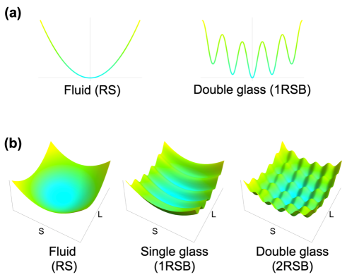
Figure 1: Schematic depiction of the free energy landscape. (a) 1RSB formalism where the horizontal axis represents the configuration of both large and small particles. (b) 2RSB formalism where the coordinates labels “L” ans “S” represent the configurations of large and small particles, respectively.

First, we consider the conventional RLT with the 1RSB ansatz (1RSB-RLT). The landscape considered in the 1RSB formalism is schematically drawn in FIG. 1 (a). In the fluid, or the replica symmetric (RS) phase, the free energy has a single minimum corresponding to equilibrium fluid, while in the 1RSB phase, the free energy has multiple minima each of which represents a different glass state. The main idea of the RLT is to introduce the $m$ copies (replicas) of the original system to distinguish the different glass states, which is referred to as the overlap. The overlap, or similarity, between the configurations of different replicas is finite within a same glass state, but zero between different minima Monasson (1995); Mézard and Parisi (1999); Biazzo et al. (2009); Parisi and Zamponi (2010). The 1RSB-RLT for monodisperse systems is well developed Parisi and Zamponi (2010) and the extension to binary mixtures is straightforward Parisi and Zamponi (2010); Biazzo et al. (2009), aside from a subtlety related to the particle exchange in a glass state Coluzzi et al. (1999); Ikeda et al. (2016); Ozawa and Berthier (2017); Ikeda et al. (2017); Ikeda and Zamponi (2019). Following the strategy of Ref. Parisi and Zamponi (2010), we introduce the density distribution function in the replica space as density of molecules made of replicas,

$$\rho_{\mu}(\underline{\bm{r}})=\sum_{i\ {\rm for}\ \mu\ {\rm particles}}\left\langle\prod_{a=1}^{m}\delta(\bm{r}^{a}-\bm{r}_{i}^{a})\right\rangle,$$ (9)

where $\underline{\bm{r}}=\{\bm{r}^{1},\cdots,\bm{r}^{m}\}$ represents the set of the particle positions in the replica space Biazzo et al. (2009); Parisi and Zamponi (2010), and $\mu\in\{L,S\}$ denotes the particle species. Expanding the free energy of the replicated system by $\rho_{\mu}(\underline{\bm{r}})$, we obtain

$$\log Z_{m} =\sum_{\mu\in\{L,S\}}\int d\underline{\bm{r}}\rho_{\mu}(\underline{\bm{r}})(1-\log\rho_{\mu}(\underline{\bm{r}})),$$

$$+\sum_{\mu\nu\in\{L,S\}}\frac{1}{2}\int d\underline{\bm{r}}d\underline{\bm{r}}^{\prime}\rho_{\mu}(\underline{\bm{r}})\rho_{\nu}(\underline{\bm{r}}^{\prime})f_{\mu\nu}(\underline{\bm{r}}-\underline{\bm{r}}^{\prime})+O(\rho^{3}),$$ (10)

where we intoduced the Mayer function defined by

$$f_{\mu\nu}(\underline{\bm{r}}-\underline{\bm{r}}^{\prime}) =\prod_{a=1}^{m}e^{-\beta v_{\mu\nu}(\bm{r}^{a}-{\bm{r}^{\prime}}^{a})}-1.$$ (11)

In the $d\to\infty$ limit, the $O(\rho^{3})$ term is negligible compared to the first and second order terms Parisi et al. (2020). Furthermore, in this limit, only the first and second cumulants of $\rho_{\mu}(\underline{\bm{r}})$ are relevant Parisi et al. (2020), meaning that Eq. (9) can be represented by the Gaussian function as Biazzo et al. (2009); Parisi and Zamponi (2010)

$$\rho_{\mu}(\underline{\bm{r}}) =\rho_{\mu}\int d\bm{R}\prod_{a=1}^{m}\gamma_{A_{\mu}}(\bm{r}^{a}-\bm{R}),$$ (12)

where $\gamma_{A}(\bm{r})=(2\pi A)^{-d/2}e^{-\frac{\left|\bm{r}\right|^{2}}{2A}}$. $A_{\mu}$ represents the strength of the correlation between $m$ replicas. This is to be determined by the saddle point condition, as described below. Substituting Eq. (12) into Eq. (10), we obtain

$$\log Z_{m}=\sum_{\mu}N_{\mu}\left[-\frac{d}{2}(1-m)\log 2\pi A_{\mu}-\frac{d}{2}(1-m-\log m)\right]$$

$$+\sum_{\mu}N_{\mu}\left(1-\log\rho_{\mu}\right)+\frac{1}{2}\sum_{\mu\nu}\frac{N_{\mu}N_{\nu}}{V}\int d\bm{r}\left(q_{\mu\nu}^{m}(\bm{r})-1\right),$$ (13)

with

$$q_{\mu\nu}(\bm{r}) =\int d\bm{R}\gamma_{A_{\mu}+A_{\nu}}(\bm{r}+\bm{R})e^{-\beta v_{\mu\nu}(\bm{R})}.$$ (14)

We first calculate the dynamical transition point $\varphi_{d}$ of our model at which the non-trivial solution of $A_{\mu}$ arises. $A_{\mu}$ can be calculated from the saddle point condition $\partial_{A_{\mu}}\log Z_{m}=0$ by taking $m\to 1$ limit for fixed $d$ and then taking the limit of $d\to\infty$ afterwards. For simplicity, below, we investigate the hard-sphere limit ($T\rightarrow 0+$). The result of monodisperse hard spheres in the large-dimension limit Parisi and Zamponi (2010) can be easily extended to binary mixtures. The saddle point condition leads to

$$\frac{1}{\hat{A}_{L}} \sim\tilde{\varphi}\left[(1-x)M(\hat{A}_{L})+xe^{r/2}M\left(\frac{\hat{A}_{L}+\hat{A}_{S}}{2}\right)\right],$$

$$\frac{1}{\hat{A}_{S}} \sim\tilde{\varphi}\left[xM(\hat{A}_{S})+(1-x)e^{-r/2}M\left(\frac{\hat{A}_{L}+\hat{A}_{S}}{2}\right)\right],$$ (15)

where we defined $\hat{A}_{\mu}=d^{2}A_{\mu}/\sigma_{\mu\mu}^{2}$ and introduced the reduced density as

$$\tilde{\varphi}=\frac{2^{d}\varphi}{d}.$$ (16)

$M(\hat{A})$ is the auxiliary function defined by

$$M(\hat{A}) =-\int dye^{y}\log\left[\Theta\left(\frac{y+\hat{A}}{\sqrt{4\hat{A}}}\right)\right]\frac{\partial}{\partial\hat{A}}\Theta\left(\frac{y+\hat{A}}{\sqrt{4\hat{A}}}\right),$$

$$\Theta(x) =\frac{1}{2}\left(1+{\rm erf}(x)\right).$$ (17)

Solving Eqs. (15) numerically, we obtain $A_{\mu}$ and $\varphi_{d}$. We show the resultant (dynamic) phase diagram in FIG. 2. When the size ratio between large and small particles, $R$ defined by Eq. (8), is small, the dynamical transitions of large and small particles take place simultaneously (see the left panel of FIG. 2). One observes only the double glass phase in which all particles are frozen. Contrarily, if $R$ is sufficiently large ($\geq R_{c}\approx 0.6$), the glass phase splits into the two phases. See the right panel of FIG. 2. At small $x$ and at modelete densities, one obtains the single glass phase in which only large particles are frozen. As the density further increases, small particles undergo the dynamical transition and enter to the double glass phase. At large $x$’s, on the contrary, the system enters to the double glass phase from the fluid phase without bypassing the slngle glass phase.

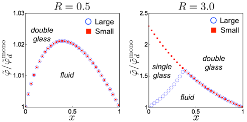
Figure 2: Dynamic phase diagram for $R=0.5$ and $R=3.0$: The circles and filled squares denote the dynamical transition points of large and small particles, respectively. The $y$-axis is scaled by the dynamical transition point of the monodisperse system, $\tilde{\varphi}_{d}^{\rm mono}$.

Next, we discuss the thermodynamic glass transition point, $\varphi_{K}$, where the configurational entropy vanishes. In the large-dimension limit, the thermodynamic glass transition density scales as $\varphi_{K}=O(2^{-d}d\log d)$ and the cage size scales as $A_{\mu}=O(1/d^{2}\log d)$ Parisi and Zamponi (2010), leading to $\gamma_{A_{\mu}}(x)\sim\delta(x)$ and $q_{\mu\nu}(r)\sim e^{-\beta v_{\mu\nu}(r)}$. Substituting this into Eq. (13), we obtain the asymptotic form of the free energy near the thermodynamic glass transition point,

$$\frac{\log Z_{m}}{Nm} =\frac{1}{m}\left[\frac{d}{2}\log d-\frac{\varphi}{2}\frac{(1-x+xe^{R/2})^{2}}{1-x+xe^{R}}I(m)\right]-d\log d,$$ (18)

where

$$I(m) =\int_{-\infty}^{\infty}\!\!\mbox{d}y~{}e^{y}\left[1-e^{-m\hat{\beta}\hat{\phi}(y)}\right]$$ (19)

with $\hat{\phi}(y)=d^{2}\phi\left(1+{y}/{d}\right)$. $\varphi_{K}$ is calculated by $\lim_{m\to 1}\Sigma(m)=0$ Parisi and Zamponi (2010), where the configurational entropy $\Sigma(m)$ is give by Eq. (4). After some manipulations, we obtain

$$\hat{\varphi}_{K}(x) =\frac{\varphi_{K}(x)}{\varphi_{K}^{\rm mono}}=\frac{1-x+xe^{R}}{(1-x+xe^{R/2})^{2}},$$ (20)

where $\varphi^{\rm mono}_{K}=2^{-d}d\log d/h(1)$ with $h(m)=-m^{2}\partial_{m}(I(m)/m)$ denotes the thermodynamic glass transition density for the one-component system. Eq. (20) implies that the thermodynamics transition point does not depend on $\beta$ and $v_{\mu\nu}$, if one uses the reduced density

$$\hat{\varphi}=\frac{\varphi}{\varphi_{K}^{\rm mono}}.$$ (21)

Typical phase diagrams predicted by Eq. (20) are shown in FIG. 3. As mentioned before, the 1RSB RLT fails to describe the decoupling of the thermodynamic glass transition points of large and small particles.

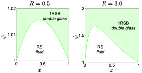
Figure 3: 1RSB phase diagram for $R=0.5$ and $R=3$: The solid line denotes the normalized thermodynamic glass transition point, $\hat{\varphi}_{K}$.

V 2RSB analysis

Next, we introduce the 2RSB ansatz into the RLT, motivated by the recent study of a binary version of mean-field spin-glass model Ikeda and Ikeda (2016). To discuss the decoupling, we separately consider the configuration of large and small particles, as shown in FIG. 1 (b). For sufficiently small $\varphi$, the system is in the RS fluid phase, where the free energy has a single minimum (FIG. 1 (b) left). For intermediate $\varphi$’s, there appears the single glass phase described by the 1RSB, where large particles are vitrified while small particles are mobile. The minimum of the free energy splits into multiple glass states due to the configuration of large particles (FIG. 1 (b) middle). For sufficiently large $\varphi$, small particles also vitrify, as a consequence, the minima further split due to the emergence of the multi-valley for the configuration of small particles (FIG. 1 (b) right). Only the 2RSB formalism can describe this hierarchical structure and the decoupling of the thermodynamic glass transition points of large and small particles. The RLT with the 2RSB ansatz is formulated by dividing $m$ replicas into $m/m_{1}$ sub-groups, each of which contains $m_{1}$ replicas. The $m_{1}$ replicas of small particles within a same sub-group are constrained around their center of mass, whereas the replicas of different sub-groups can move independently. For large particles, all $m$ replicas are constrained around their center of mass. In other words, the replicated liquid is a $(m/m_{1}+1)$-component molecular mixture which consists of $m/m_{1}$ types of molecules composed of $m_{1}$ small particles and one type of molecules composed of $m$ large particles. Note that the higher order RSB is a natural consequence of consecutive transitions of each component, and this picture is distinct from the full RSB transition recently studied in the context of the marginal glass transition where each RSB state corresponds to one frozen state Charbonneau et al. (2014).

Based on the 2RSB ansatz, one can write down the free energy of the replica liquid using the virial expansion of the standard grand canonical partition function, which reads

$$\log Z_{m}=\int\mbox{d}\underline{\bm{r}}\rho_{L}(\underline{\bm{r}})(1-\log\rho_{L}(\underline{\bm{r}}))+\sum_{k=1}^{m/m_{1}}\int\mbox{d}\underline{\bm{r}}^{k}\rho_{S_{k}}(\underline{\bm{r}}^{k})(1-\log\rho_{S_{k}}(\underline{\bm{r}}^{k}))+\frac{1}{2}\int\mbox{d}\underline{\bm{r}}d\underline{\bm{r}}^{\prime}\rho_{L}(\underline{\bm{r}})\rho_{L}(\underline{\bm{r}}^{\prime})f_{LL}(\underline{\bm{r}}-\underline{\bm{r}}^{\prime})$$

$$+\sum_{k=1}^{m/m_{1}}\frac{1}{2}\int\mbox{d}\underline{\bm{r}}^{k}d\underline{\bm{r}}^{\prime k}\rho_{S_{k}}(\underline{\bm{r}}^{k})\rho_{S_{k}}(\underline{\bm{r}}^{\prime k})f_{SS}(\underline{\bm{r}}^{k}-\underline{\bm{r}}^{\prime k})+\sum_{k=1}^{m/m_{1}}\int\mbox{d}\underline{\bm{r}}d\underline{\bm{r}}^{\prime k}\rho_{L}(\underline{\bm{r}})\rho_{S_{k}}(\underline{\bm{r}}^{\prime k})f_{LS}(\underline{\bm{r}}^{k}-\underline{\bm{r}}^{\prime k})+O(\rho_{L}^{3},\rho_{S_{k}}^{3}).$$ (22)

In this expression, $\rho_{S_{k}}$ is the density field of small particles of the $k$-th type  . $\underline{\bm{r}}=\{\bm{r}^{1},\cdots,\bm{r}^{m}\}$ and $\underline{\bm{r}}^{k}=\{\bm{r}^{1,k},\cdots,\bm{r}^{m_{1},k}\}$ represent their coordinates in the replica space. $f_{\mu\nu}(\underline{\bm{r}}-\underline{\bm{r}}^{\prime})$ $(\mu,\nu\in L,S_{k})$ is the Mayer function defined by

$$f_{\mu\nu}(\underline{\bm{r}}-\underline{\bm{r}}^{\prime}) =\prod_{a}e^{-\beta v_{\mu\nu}(\bm{r}^{a}-\bm{r}^{\prime,a})}-1,$$ (23)

where the product over $a$ is made only for the replicas commonly included in the $\mu$ and $\nu$ molecules. The first and second terms of Eq. (22) are the ideal gas parts and the third to fifth terms represent the interaction contributions Parisi and Zamponi (2010). As before, we give the profiles of $\rho_{L}(\underline{\bm{r}})$ and $\rho_{S_{k}}(\underline{\bm{r}}^{k})$ as Gaussian Parisi and Zamponi (2010), which is known to be exact in the large-dimension limit Kurchan et al. (2012).

It should be emphasized that, in the large-dimension limit, only the lowest order term in the Mayer expansions survives, which simplifies the analysis considerably. This implies that, in the large-dimension limit, the so-called depletion force, a short-ranged attraction between large particles induced by small ones, is absent Asakura and Oosawa (1954); Dijkstra et al. (1999), which is intrinsically the higher order effect.

The glass phases are determined by optimizing the free energy, Eq. (22), with respect to $m$, $m_{1}$, and the cage sizes. The thermodynamic glass transition density $\varphi_{K}$ is the point at which the configurational entropy vanishes. In the vicinity of $\varphi_{K}\sim O(d\log d)$ Parisi and Zamponi (2010), the free energy can be simplified and written by an asymptotic expression

$$\frac{\log Z_{m}}{Nm} =g_{1}(m)+g_{2}(m_{1})-d\log d,$$ (24)

with the auxiliary functions defined by

$$g_{1}(m) =\frac{1}{m}\bigg{[}\frac{1-x}{1-x+xe^{R}}\frac{d}{2}\log d-\frac{2^{d}\varphi}{2}\frac{(1-x)^{2}}{1-x+xe^{R}}I(m)\bigg{]},$$

$$g_{2}(m_{1}) =\frac{1}{m_{1}}\bigg{[}\frac{xe^{R}}{1-x+xe^{R}}\frac{d}{2}\log d$$

$$-\frac{2^{d}\varphi}{2}\frac{x^{2}e^{R}+2x(1-x)e^{R/2}}{1-x+xe^{R}}I(m_{1})\bigg{]}.$$ (25)

Inside the glass phases, $\varphi>\varphi_{K}$, $m$ and $m_{1}$ become smaller than unity. There are two possibilities, $m<m_{1}<1$ and $m=m_{1}<1$, which should be treated separately.

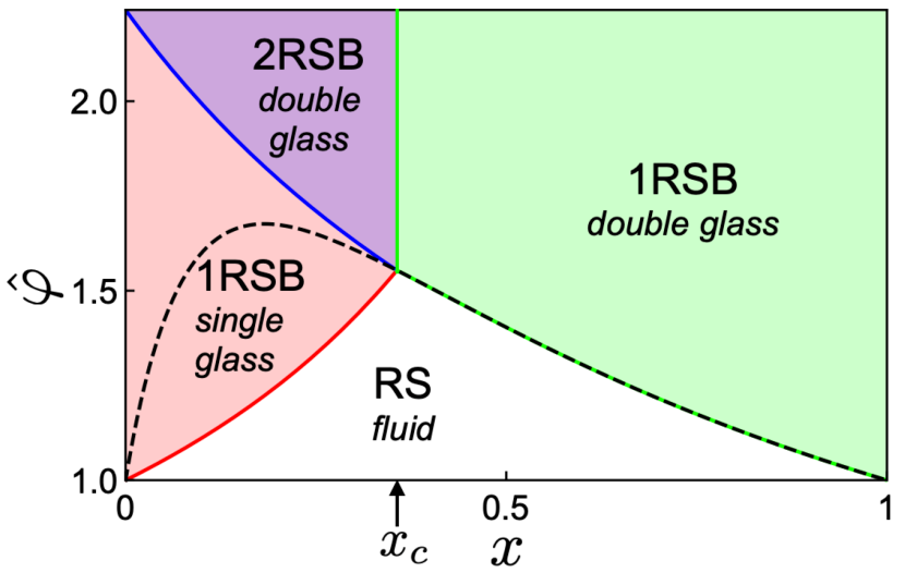
Figure 4: Full phase diagram for $R=3$. $x$ is the concentration fraction of small particles. $\hat{\varphi}$ is the packing fraction divided by the glass transition point of the one-component system. The broken line is the glass transition line obtained by the 1RSB-RLT.

In the case of $m<m_{1}<1$, the glass phase is characterized by the 2RSB free energy (FIG. 1 (b)). $m$ and $m_{1}$ are determined by solving the saddle point equations, $\Sigma_{1}=0$ and $\Sigma_{2}=0$. Substituting Eq. (24) into Eqs. (7), we get

$$\frac{h(m)}{h(1)} =\frac{\varphi_{K}^{\rm mono}}{\varphi(1-x)},~{}~{}\frac{h(m_{1})}{h(1)}=\frac{\varphi_{K}^{\rm mono}}{\varphi\left[x+2(1-x)e^{-R/2}\right]}.$$ (26)

$\varphi_{K}$ for large particles is obtained as the 1RSB solution by setting $m=1$ in the first equation of Eq. (26) as

$$\varphi_{K}^{\rm 1RSB}(x) =\frac{\varphi_{K}^{\rm mono}}{1-x}.$$ (27)

Similarly, $\varphi_{K}$ for small particles is obtained as the 2RSB solution by setting $m_{1}=1$ in the second equation of Eq. (26);

$$\varphi_{K}^{\rm 2RSB}(x) =\frac{\varphi_{K}^{\rm mono}}{x+2(1-x)e^{-R/2}}.$$ (28)

In the case of $m=m_{1}<1$, on the other hand, the glass phase is described by the 1RSB free energy (see Sec. IV). The 1RSB and 2RSB free energies become identical when the fraction is

$$x_{c}=\frac{1-2e^{-R/2}}{2(1-e^{-R/2})}.$$ (29)

This equation determines the phase boundary between the 1RSB and 2RSB glass phases. When $x<x_{c}$, the 2RSB phase is more stable than 1RSB phase and vice versa for $x>x_{c}$. For $x_{c}$ to be positive, $R$ must be larger than $R_{c}=2\log 2$, which is the necessary condition for the 2RSB phase or equivalently the decoupling of the two glass transitions. Note that all the arguments above are independent of the temperature and shape of the potential $v_{\mu\nu}(r)$, as it is obvious by rescaling the density by

$$\hat{\varphi}=\frac{\varphi}{\varphi_{K}^{\rm mono}}.$$ (30)

Combining all results discussed above, we draw the thermodynamic glass phase diagram. If $R<R_{c}$, the phase diagram is determined by the 1RSB-RLT and only a single glass phase exists. If $R>R_{c}$, four different phases emerge as shown in FIG. 4. At very low densities, the system is in the RS (fluid) phase where the solution with $m=m_{1}=1$ is the most stable. If $\varphi$ is large and $x$ is close to $1$, the solution with $m=m_{1}<1$ is the most stable, and the system is in the 1RSB phase where all particles are frozen. We refer to this phase as the 1RSB double glass phase. In this phase, the majority is small particles, and they drive the system into the glass phase. In other words, large particles are embedded in vitrified small particles. Indeed, $\varphi_{K}(x)$ smoothly converges to $\varphi_{K}^{\rm mono}$ in the one-component limit, $x\to 1$. As $x$ decreases and crosses $x_{c}$, the system undergoes the transition from the 1RSB ($m=m_{1}<1$) to 2RSB ($m<m_{1}<1$). We refer to this phase as the 2RSB double glass. As $x$ decreases further, $m<m_{1}=1$ becomes stable and small particles melt into a fluid phase whereas large particles remain frozen. We refer to this phase as the 1RSB single glass. The difference between the 1RSB and 2RSB double glass phases should be emphasized.

As the density is increased for a fixed $x$ below $x_{c}$, the system undergoes the two step glass transitions: first from the fluid to the 1RSB single glass and then to the 2RSB double glass phase. In order to clarify the nature of this multiple transitions, we calculate the configurational entropy, $\Sigma$, from the 2RSB free energy given by Eq. (22). It can be written as a sum of the two contribution, $\Sigma=\Sigma_{1}+\Sigma_{2}$ Obuchi et al. (2010). Here $\Sigma_{1}$ is the configurational entropy of large particles corresponding to the large metabasins generated by large particles. $\Sigma_{2}$ is the configurational entropy of small particles corresponding to the basins inside the one of the metabasins. We evaluate $\Sigma$ using the asymptotic expression of the free energy, Eq. (24), and Eqs. (7). FIG. 5 is the density dependence of $\Sigma$ for $R=3$ and $x=0.2$. The result of the (meta-stable) 1RSB solution is also shown with the dashed line for a reference. One observes that $\Sigma$ bends twice; first at $\hat{\varphi}_{K}^{\rm 1RSB}$, where $\Sigma_{1}$ vanishes and the second at $\hat{\varphi}_{K}^{\rm 2RSB}$, where $\Sigma_{2}$ vanishes, and thus the whole configurational entropy dies out.

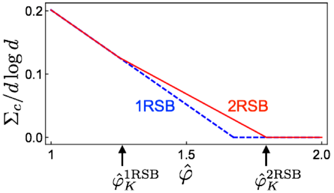
Figure 5: The density dependence of the configurational entropy for $R=3$ and $x=0.2$ which is smaller than $x_{c}<0.36$. The solid and dashed lines represent the 2RSB and 1RSB results, respectively. The arrows indicates the transition point from the fluid to 1RSB(2) and the transition point from the 1RSB(2) to 2RSB phases.

VI Summary and conclusions

In summary, we developed a new formalism of the RLT for binary mixtures of large and small particles based on the 2RSB ansatz. We determined the glass phase diagram for a hardsphere-like fluid in infinite dimension. The theory predicts that when the size ratio $R$ is larger than a critical value, $R_{c}$, the hierarchical energy landscape emerges and the decoupling of the glass transition of large and small particles takes place. As a consequence, there arise several distinct glass phases: the 1RSB double glass, 1RSB single glass, and the 2RSB double glass phases.

It should be addressed that the 1RSB and 2RSB double glasses are distinct phases with qualitative and topographical differences in their free energy landscapes. The energy landscape in the 2RSB phase has the two-step hierarchical structure where the two levels correspond to the configurations of large and small particles, respectively. It is desirable to design experimental setup or simulation method which allows to delineate the difference of the two phases. We suspect that a mechanical response or nonlinear rheology measurement would be one of ideal candidates Shikata (2001); Pham et al. (2006); Koumakis and Petekidis (2011); Yoshino and Zamponi (2014). For example, an anomalous two-step yielding in colloidal binary mixtures has been reported Sentjabrskaja et al. (2013), which may be a reflection of complex and hierarchical energy landscape. Note that in a recent simulation study of hard-spheres near the jamming transition, two glass phases characterized by different status of the replica symmetry breaking are indeed separated well by rheological measurement Jin and Yoshino (2017). The shape of the phase diagram predicted by our theory is qualitatively consistent with experiment and numerical results Imhof and Dhont (1995a, b); Moreno and Colmenero (2006a, b); Hendricks et al. (2015); the single glass phase is located at high density and small $x$ region while the double glass phase is at high density and large $x$ region. For more quantitative comparison, it is necessary to extend our theory to finite dimensions.

The relationship of our theory with the MCT, on the other hand, remains somewhat elusive. First, our theory does not distinguish the self and collective density correlations, in contrast to the MCT in finite $d$. This simplifies the analysis but simultaneously reduces the diversity of the phase diagram. Second, the MCT is usually identified with the dynamical transition point of the replica liquid theory . However our theory shows that the description of the single and double glass phases at smaller $x$ requires the 2RSB ansatz. This means that the nature of the decoupling predicted by the MCT is essentially different from those of thermodynamic theory.

We believe that our higher order replica symmetric breaking picture is not restricted to binary mixtures of disparate size ratios, but can be adapted for other decoupling phenomena of the glass transitions, e.g., the decoupling of translational and rotational motions in anisotropic particles. These are left for the future work.