The three-dimensional structure of swirl-switching in bent pipe flow

Abstract

Swirl-switching is a low-frequency oscillatory phenomenon which affects the Dean vortices in bent pipes and may cause fatigue in piping systems. Despite thirty years worth of research, the mechanism that causes these oscillations and the frequencies that characterise them remain unclear. Here we show that a three-dimensional wave-like structure is responsible for the low-frequency switching of the dominant Dean vortex. The present study, performed via direct numerical simulation, focuses on the turbulent flow through a $90^{\circ}$ pipe bend preceded and followed by straight pipe segments. A pipe with curvature $0.3$ (defined as ratio between pipe radius and bend radius) is studied for a bulk Reynolds number $\Rey=11\,700$, corresponding to a friction Reynolds number $\Rey_{\tau}\approx 360$. Synthetic turbulence is generated at the inflow section and used instead of the classical recycling method in order to avoid the interference between recycling and swirl-switching frequencies. The flow field is analysed by three-dimensional proper orthogonal decomposition (POD) which for the first time allows the identification of the source of swirl-switching: a wave-like structure that originates in the pipe bend. Contrary to some previous studies, the flow in the upstream pipe does not show any direct influence on the swirl-switching modes. Our analysis further shows that a three-dimensional characterisation of the modes is crucial to understand the mechanism, and that reconstructions based on 2D POD modes are incomplete.

1 Introduction

Bent pipes are an essential component of a large number of industrial machines and processes. They are ideal for increasing mass and momentum transfer, passively mixing different fluids, which makes them effective as heat exchangers, inverters, and other appliances. For a review of the applications of bent pipes in industry see Vashisth et al. (2008); the most recent advances in experiments and simulations can be found in the review by Kalpakli Vester et al. (2016). The high mass and momentum transfer is generated by the secondary motion caused by the centrifugal force acting on the fluid in the curved sections. This secondary motion, which is of Prandtl’s first kind, takes the shape of two counter-rotating vortices, illustrated in figure 1, which move the fluid towards the outside of the bend, along the centreline, and back towards the inside along the wall, therefore increasing the mass and momentum transfer across the pipe section.

These vortices were first observed by Boussinesq (1868) and Eustice (1910), and later described analytically by Dean (1928) from whom they received the name of Dean vortices. The intensity of these vortices increases with Reynolds number, here based on pipe diameter and bulk velocity (i.e., $\Rey=DU_{b}/\nu$, where $\nu$ is the kinematic viscosity of the fluid), as well as with pipe curvature, defined as the ratio between pipe radius and bend radius, $\delta=R/R_{c}$ (see Canton et al. 2017 for laminar flow; Noorani et al. 2013, the review by Kalpakli Vester et al. 2016, and references therein, for turbulent flows).

For laminar, steady flow the Dean vortices are symmetric with respect to the bend symmetry plane (the $I$-$O$ plane in figure 1); but when the flow becomes unstable the vortices start oscillating periodically (Kühnen et al., 2014, 2015; Canton et al., 2016). These large-scale oscillations are caused by the appearance of periodic travelling waves which, as also observed in other flows (see, e.g. Hof et al., 2004), are at the base of transition to turbulence for toroidal and helical pipes.

A different kind of large-scale oscillations is observed for high Reynolds numbers: here the turbulent flow is modulated by a low-frequency alternation of the dominant Dean vortex. This vortex alternation excites the pipe structure and is presumed to be the cause of structural, low-frequency oscillations observed in heat exchangers (e.g. in microgravity conditions such as in a test for the international space station; Brücker, 1998), as well as the origin of secondary motion in the bends of the cooling system of nuclear reactors (Kalpakli Vester et al., 2016). The Dean vortex alternation was initially, and unexpectedly, observed by Tunstall & Harvey (1968), who experimentally studied the turbulent flow through a sharp, L-shaped bend ($\delta=1$). These authors measured “low random-frequency” switches between two distinct states and, by means of flow visualisations, were able to identify an either clockwise or anti-clockwise predominance of the swirling flow following the bent section. The switching was found to have a Strouhal number $St=fD/U_{b}$ highly dependent on $\Rey$ and comprised between $2\times 10^{-4}$ and $4.5\times 10^{-3}$. Tunstall & Harvey attributed the origin of the switching to the presence of a separation bubble in the bend and to the “occasional existence of turbulent circulation entering the bend”.

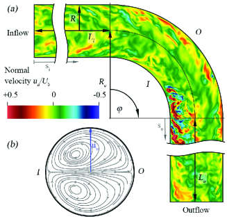
Figure 1: Schematic of the computational domain. (a) A section of the pipe with curvature $\delta=R/R_{c}=0.3$, including the definition of the geometrical parameters and an instantaneous flow field coloured by normal velocity, i.e., normal to the bend symmetry plane. (b) Streamlines of the mean cross-flow showing the Dean vortices on a cross-section extracted at $s_{o}=0$. An animated view of the setup is provided in the supplementary online material, movie1.m4v.

To the best of our knowledge, the first author to continue the work by Tunstall & Harvey (1968) was Brücker (1998), who analysed the phenomenon via particle image velocimetry (PIV) and coined the term “swirl-switching”. Brücker studied a smoothly curved pipe with $\delta=0.5$ and identified the oscillations as a continuous transition between two mirror-symmetric states with one Dean cell larger than the other. He confirmed that the switching takes place only when the flow is turbulent, and he reported two distinct peaks, $St=0.03$ and $0.12$, at frequencies considerably higher than those measured by Tunstall and Harvey, despite the lower Reynolds numbers considered.

Rütten et al. (2001, 2005) were the first to numerically study swirl-switching by performing large-eddy simulations (LES) for $\delta=0.167$ and $0.5$. The main result of this analysis is that the switching takes place even without flow separation; moreover, Rütten and co-workers found that the structure of the switching is more complex than just the alternation between two distinct symmetric states, since the outer stagnation point “can be found at any angular position within $\pm 40^{\circ}$”. Rütten et al. found a high-frequency peak at $St\approx 0.2$, attributed to a shear-layer instability, and, only for their high Reynolds number case, one low-frequency peak for $St\approx 5.5\times 10^{-3}$, which was connected to the swirl-switching. However, the simulations for Rütten et al.’s work were performed by using a “recycling” method, where the results from a straight pipe simulation were used as inflow condition for the bent pipe. These periodic straight pipes were of length $L=3.5D$ and $5D$ and likely influenced the frequencies measured in the bent pipes since the periodicity of the straight pipes introduced a forcing for $St=U_{b}/L=1/3.5$ and $1/5$, respectively.

Sakakibara et al. (2010) were the first to analyse the flow by means of two-dimensional proper orthogonal decomposition (2D POD) performed on snapshots extracted from stereo PIV. Their results for $\delta=0.75$ reveal anti-symmetric structures that span the entire pipe cross-section and contain most of the energy of the flow. A spectral analysis of the corresponding time coefficients shows peaks between $St\approx 0.07$ at $s_{o}=2D$ and $St\approx 0.02$ for $s_{o}=25D$, in the range found by Brücker (1998). In a subsequent work Sakakibara & Machida (2012) conjectured that the swirl-switching is caused by very large-scale motions (VLSM) formed in the straight pipe preceding the bend.

Hellström et al. (2013) and Kalpakli & Örlü (2013) also presented results based on 2D POD. The former performed experiments for $\delta=0.5$ and found non-symmetric modes resembling a tilted variant of the Dean vortices with $St=0.16$ and $0.33$, corresponding to the shear-layer instabilities found by Rütten et al. (2005). Kalpakli & Örlü (2013), on the other hand, studied a pipe with $\delta=0.31$; differently from previous works, the section of straight pipe following the bend was only $0.67$ diameters long. Their results at the exit of this short segment show clearly antisymmetric modes as most dominant structures. The swirl-switching frequency obtained from the POD time coefficients was $St=0.04$; peaks of $St=0.12$ and $0.18$ were also measured but were found not to be related to swirl-switching. In a later work Kalpakli Vester et al. (2015) repeated the experiments for $\delta=0.39$ and found again a dominant frequency corresponding to $St=0.04$.

Carlsson et al. (2015) performed LES in a geometry similar to that of Kalpakli & Örlü (2013), namely, with a short straight section following the bend, for four different curvatures. The inflow boundary condition was generated by means of a recycling method, as in Rütten et al. (2001, 2005), with a straight pipe of length $7D$, exciting the flow in the bent pipe at $St=1/7$. The three lower curvatures were therefore dominated by the spurious frequencies artificially created in the straight pipe by the recycling method, while the frequencies measured for $\delta=1$, corresponding to $0.5<St<0.6$, were in the same range identified by Hellström et al. (2013) but were found to be mesh dependent.

Noorani & Schlatter (2016) were the first to investigate the swirl-switching by means of direct numerical simulations (DNS). By using a toroidal pipe they showed that swirl-switching is not caused by structures coming from the straight pipe preceding the bend, but is a phenomenon inherent to the curved section. Two curvatures were investigated, $\delta=0.1$ and $0.3$, and both presented a pair of antisymmetric Dean vortices as the most energetic POD mode with $St=0.01$ and $0.087$.

Table 1 summarises the main results of the aforementioned studies. It is clear from this literature review that there is a strong disagreement among previous works not only on what is the mechanism that leads to swirl-switching, but also on what is the frequency that characterises this phenomenon. In the present work an answer to both questions will be given, which will also explain the discrepancies between previous studies.

The paper continues with a description of the numerical methods employed for the analysis, presented in §2, devoting special attention to the inflow boundary conditions. The results of the simulations and POD analysis are presented in §3 and are discussed and compared with the literature in §4.

Reference	$\delta$	$\Rey$	$St$
Tunstall & Harvey (1968)	$1$	$50\,000$ – $230\,000$	$2\times 10^{-4}$ – $4.5\times 10^{-3}$
Brücker (1998)	$0.5$	$5\,000$	$0.03$, $0.12$
Rütten et al. (2001, 2005)	$0.167$, $0.5$	$27\,000$	$5.5\times 10^{-3}$
Sakakibara et al. (2010)	$0.75$	$120\,000$	$0.02$ – $0.07$
Hellström et al. (2013)	$0.5$	$25\,000$	$0.16$, $0.33$
Kalpakli & Örlü (2013)	$0.31$	$34\,000$	$0.04$
Kalpakli Vester et al. (2015)	$0.39$	$24\,000$	$0.04$
Carlsson et al. (2015)	$0.32$, $0.5$, $0.7$, $1$	$34\,000$	$0.003$ – $0.01$, $0.13$, $0.5$ – $0.6$
Noorani & Schlatter (2016)	$0.1$, $0.3$	$11\,700$	$0.01$, $0.087$

Table 1: Reference Strouhal numbers measured in previous studies and attributed to swirl-switching. The analysis in the present work is performed at $\Rey=11\,700$ in a bent pipe with curvature $\delta=0.3$.

2 Analysis methods

2.1 Numerical discretisation

The present analysis is performed via DNS of the incompressible Navier–Stokes equations. The equations are discretised with the spectral-element code Nek5000 (Fischer et al., 2008) using a $\mathbb{P}_{N}-\mathbb{P}_{N-2}$ formulation. After an initial mesh-dependency study, the polynomial order was set to $N=8$ for the velocity and, consequently, $N=6$ for the pressure. We consider a $90^{\circ}$ bent pipe with curvature $\delta=0.3$ for a Reynolds number $\Rey=11\,700$, corresponding to a friction Reynolds number $\Rey_{\tau}\approx 360$ (referred to the straight pipe sections). A straight pipe of length $L_{i}=7D$ precedes the bent section (see §3.1), and a second straight segment of length $L_{o}=15D$ follows it. Further details about the mesh, including element number and size, are reported in table 2. The supplementary video movie1.m4v shows the setup and a visualization of the flow.

	$n_{\mathrm{el}}$	$n_{\mathrm{dof}}$	$\Delta r^{+}$	$\Delta(R\theta)^{+}$	$\Delta z^{+}$
$\delta=0.3$	$480\,000$	$595\,258\,500$	$(0.56,4.89)$	$(2.26,4.40)$	$(0.93,10.29)$

Table 2: Details of the mesh employed in the present work. $n_{\mathrm{el}}$ corresponds to the number of hexahedral elements, while $n_{\mathrm{dof}}$ is the total number of degrees of freedom (velocity and pressure). Quantities indicated as $(\cdot)^{+}$ are reported in viscous scaling, and the numbers between parenthesis correspond to minimum and maximum values.

2.2 Inflow boundary and divergence-free synthetic eddy method

Since the aim of the present work is to reproduce and study swirl-switching, a periodic or quasi-periodic phenomenon, the treatment of the inflow boundary is of utmost importance. The flow field prescribed at the inflow boundary should not introduce any artificial frequency, in order to avoid the excitation of unphysical phenomena or a modification of the frequencies inherent to the swirl-switching. A recycling method, as the one used by Rütten et al. (2001, 2005) and Carlsson et al. (2015), should therefore be avoided, as highlighted in §1.

In the present work the velocity field at the inlet boundary of the straight pipe preceding the bend is prescribed via a divergence-free synthetic eddy method (DFSEM). This method, introduced by Poletto et al. (2011) and based on the original work by Jarrin et al. (2006), works by prescribing a mean flow modulated in time by fluctuations in the vorticity field. The superposition of the two reproduces up to second order the mean turbulent fluctuations of a reference flow and requires a short streamwise adjustment length to fully reproduce all quantities. The fluctuations are provided by a large number of randomly distributed “vorticity spheres” (or “eddies”) which are generated and advected with the bulk velocity in a fictitious cylindrical container located around the inflow section. When a sphere exits the container, a new, randomly located sphere is created to substitute it. The cylindrical container is dimensioned such that newly created eddies do not touch the inlet plane upon their creation and they have stopped affecting it before exiting the container, i.e., the cylinder extends from $-\max(D_{\text{eddies}})$ to $\max(D_{\text{eddies}})$ (see figure 5 in Poletto et al., 2013, for an illustration of the container).

The random numbers required to create the fluctuations are generated on a single processor with a pseudo random number generator (Chandler & Northrop, 2003) featuring an algorithmic period of $2^{1376}$ iterations, large enough to exclude any periodicity in the simulations, which feature approximately $10\,000$ synthetic eddies. The size of the spheres is selected to match the local integral turbulence length scale, and their intensity is scaled to recover the reference turbulent kinetic energy, producing isotropic but heterogeneous second-order moments. The method prescribes isotropic turbulence, instead of the correct anisotropic variant, because it was shown that the former leads to a shorter adjustment length in wall-bounded flows (see figure 11 in Jarrin et al., 2006). In order to satisfy the continuity equation, no synthetic turbulence is created below $(R-r)^{+}<10$; however, this does not significantly affect the adjustment length since the dynamics of the viscous sublayer are faster than the mean and converge to a fully developed state in a shorter distance. The turbulence statistics necessary for the method, specifically the mean flow $U(r)$, the turbulent kinetic energy $k(r)$, and the dissipation rate $\epsilon(r)$, were extracted from the straight pipe DNS performed by El Khoury et al. (2013). Section 3.1 presents the validation of our implementation of the DFSEM; more details can be found in Hufnagel (2016).

2.3 Proper orthogonal decomposition

Besides point measures, we use POD (Lumley, 1967) to extract coherent structures from the DNS flow fields and identify the mechanism responsible for swirl-switching. More specifically, we use snapshot POD (Sirovich, 1987) where $n$ three-dimensional, full-domain flow fields of dimension $d$ (corresponding to the number of velocity unknowns) are stored as snapshots. POD decomposes the flow in a set of orthogonal spatial modes $\boldsymbol{\varPhi}_{i}(\boldsymbol{x})$ and corresponding time coefficients $a_{i}(t)$ ranked by kinetic energy content, in decreasing order. The most energetic structure extracted by POD corresponds to the mean flow and will be herein named “zeroth mode”, while the term “first mode” will be reserved for the first time-dependent structure.

A series of instantaneous flow fields (snapshots) is ordered column-wise in a matrix $\boldsymbol{S}\in\mathbb{R}^{d\times n}$ and decomposed as:

$$\boldsymbol{S}=\boldsymbol{U}\boldsymbol{\Sigma}\boldsymbol{V}^{\intercal}=\sum_{i=1}^{d}\boldsymbol{\varPhi}_{i}a_{i},$$ (1)

where $\boldsymbol{U}\in\mathbb{R}^{d\times d}$, $\boldsymbol{\Sigma}=diag(\sigma_{1},\sigma_{2},\cdots,\sigma_{m},0)$, with $m=\min(d,n)$, and $\boldsymbol{V}\in\mathbb{R}^{n\times n}$. The decomposition in (1) is obtained by computing the singular value decomposition (SVD) of $\boldsymbol{M}^{1/2}\boldsymbol{S}\boldsymbol{T}^{1/2}$, where $\boldsymbol{M}$ is the mass matrix and $\boldsymbol{T}$ is the temporal weights matrix, which results in $\tilde{\boldsymbol{U}}\boldsymbol{\Sigma}\tilde{\boldsymbol{V}}^{\intercal}$, where $\tilde{\boldsymbol{U}}$ and $\tilde{\boldsymbol{V}}$ are unitary matrices ($\tilde{\boldsymbol{U}}^{\intercal}\tilde{\boldsymbol{U}}=\boldsymbol{I}$ and $\tilde{\boldsymbol{V}}^{\intercal}\tilde{\boldsymbol{V}}=\boldsymbol{I}$); the POD modes are then obtained as $\boldsymbol{U}=\boldsymbol{M}^{-1/2}\tilde{\boldsymbol{U}}$ and $\boldsymbol{V}=\boldsymbol{T}^{-1/2}\tilde{\boldsymbol{V}}$. To improve the convergence of the decomposition, we exploit the symmetry of the pipe about the $I-O$ plane, which results into a statistical symmetry for the flow, and store an additional mirror image for each snapshot (Berkooz et al., 1993).

3 Results and analysis

3.1 Inflow validation

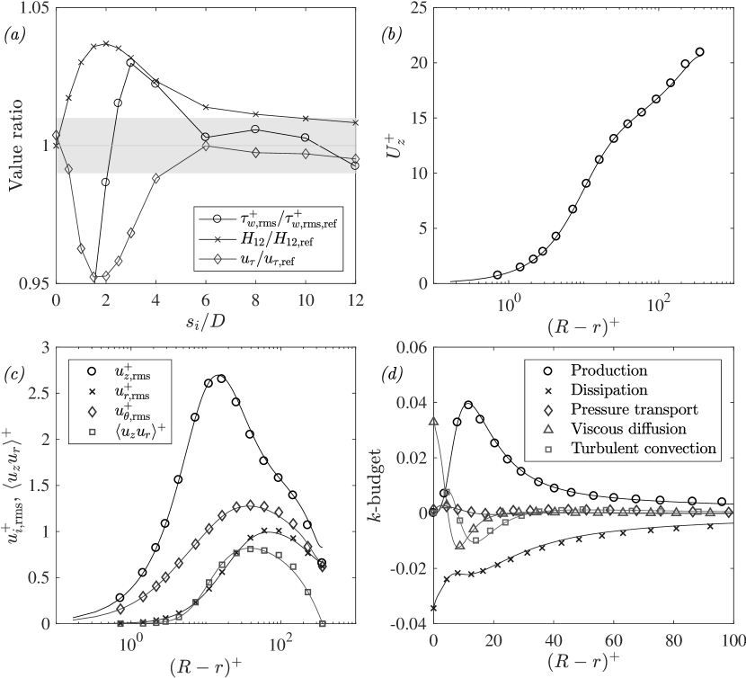
Figure 2: Recovery of fully developed turbulence statistics for the divergence-free synthetic eddy method at $\Rey_{\tau}=360$, compared to the reference values by El Khoury et al. (2013). Panel (a) shows the ratio between the DFSEM and the reference data as a function of streamwise distance from the inflow plane. The grey shaded area indicates a $\pm 1\%$ tolerance with respect to the data by El Khoury et al. (2013). Panels (b-d) show classical statistical profiles as a function of radial position at $s_{i}=5D$. Solid lines indicate the reference data, while symbols represent the current results (note that the number of shown points is reduced and does therefore not represent the grid resolution; see table 2).

An auxiliary simulation for $\Rey_{\tau}=360$ was set up to test the performance of the DFSEM in a $25D$ long straight pipe, provided with the same mesh characteristics used for the bent pipes. Classical statistical quantities were used for the validation and compared with the reference values by El Khoury et al. (2013). The comparison is presented in figure 2(a) as a function of distance from the inflow boundary, and shows that the DFSEM approaches a fully developed turbulent state (within $\pm 1\%$ of error) at approximately $5D$ from the inflow boundary. Figures 2(b-d) present the velocity, stress profiles, and the turbulent kinetic energy budget at the chosen streamwise position of $s_{i}=5D$, which confirm the recovery of fully developed turbulence by the divergence-free synthetic eddy method.

A length of $7D$ was therefore chosen for the straight pipe preceding the bent section, in order to allow for some tolerance and to account for the (weak, up to $1D$) upstream influence of the Dean vortices (Anwer et al., 1989; Sudo et al., 1998). For comparison, the more commonly used approach where random noise is prescribed at the inflow requires a development length between $50$ and $110D$ (Doherty et al., 2007). POD modes were also computed to further check the correctness of this method. The results, not reported here for conciseness, were in good agreement with those presented by Carlsson et al. (2015) for a periodic straight pipe, that is, streamwise invariant modes with azimuthal wavenumbers between $3$ and $7$.

3.2 Two-dimensional POD

Two-dimensional POD, considering all three velocity components, is employed as a first step in the analysis of swirl-switching. Instantaneous velocity fields are saved at a distance of $2D$ from the end of the bent section and are used, with their mirror images, to assemble the snapshot matrices (Berkooz et al., 1993). $1\,234$ velocity fields were saved at a sampling frequency of $St=0.25$, and the sampling was started only after the solution had reached a statistically steady state. As a consequence of exploiting the mirror symmetry, all modes are either symmetric or antisymmetric, a condition to which they would converge provided that a sufficient number of snapshots had been saved.

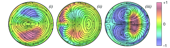
Figure 3: Pseudocolor of the streamwise velocity component and streamlines of the in-plane velocity components for the first three POD modes (i–iii). The modes are oriented as in figure 1(b). The snapshots were extracted at $s_{o}=2D$.

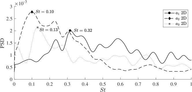
Figure 4: Welch’s power spectral density estimate for the time coefficients $a_{i}$ of the most energetic 2D POD modes. The frequencies are scaled with pipe diameter and bulk velocity. The 2D modes were extracted at $s_{o}=2D$. The markers and corresponding labels report the frequency of the highest peak of each spectrum.

The first three modes are shown in figure 3 by means of pseudocolors of their streamwise velocity component and streamlines of the in-plane velocity components. Two out of three modes are antisymmetric: (i, ii) and are in the form of a single swirl covering the whole pipe section, (i), and a double swirl, (ii), formed by two counter-rotating vortices disposed along the inner-outer direction on the symmetry plane. The third mode, (iii), resembles a harmonic of the Dean vortices.

These findings are in agreement with previous experimental work, such as that of Sakakibara et al. (2010) and Kalpakli & Örlü (2013), which attributed the dynamics of swirl-switching to the antisymmetric modes. The frequency content of these modes is presented in figure 4, in terms of Welch’s power spectral density estimate for the time coefficients of the first three modes, corresponding to the structures shown in figure 3. It can be observed that the spectra have a low peak-to-noise ratio and that each mode is characterised by a different spectrum and peak frequency, in agreement with previous 2D POD studies: see, e.g., figure 8 in Hellström et al. (2013), which presents peaks with similar values to the present ones, although their study was for a slightly larger curvature of $\delta=0.5$. This fact has caused some confusion in the past, with disagreeing authors attributing different causes to the various peaks, without being able to come to the same conclusion about the frequency, nor the structure, of swirl-switching. The reason is that swirl-switching is caused by a three-dimensional wave-like structure, as will be shown by 3D POD in §3.3, and a two-dimensional cross-flow analysis cannot distinguish between the spatial and temporal amplitude modulations created by the passage of the wave. A simple analytical demonstration of this concept is provided in the Appendix, and shows that conclusions drawn from a flow reconstruction based on 2D POD modes (see, e.g., Hellström et al., 2013) are incomplete.

3.3 Three-dimensional POD

For the 3D POD, the same snapshots as for 2D POD were used. In order to reduce memory requirements, the snapshots were interpolated on a coarser mesh before computing the POD. This is, however, not a problem because the swirl-switching is related to large-scale fluctuations in the flow.

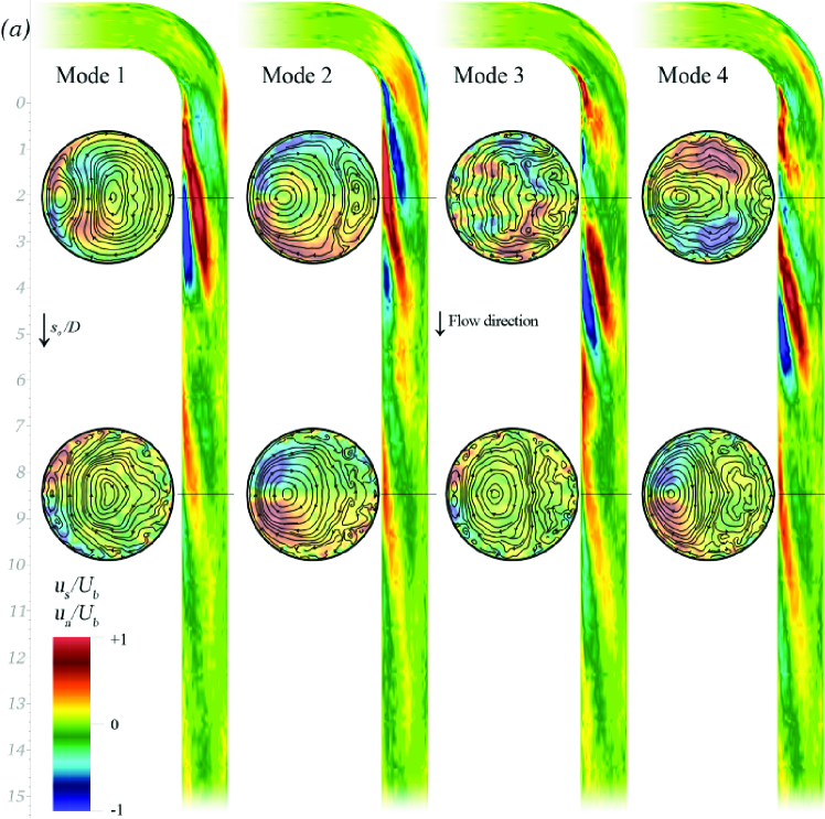
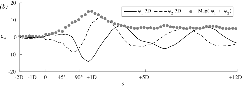
Figure 5: Panel (a) shows the four most energetic three-dimensional POD modes. The four longitudinal cuts show pseudocolours of the normal velocity component $u_{n}$, while the eight cross-sections display the in-plane streamlines and are coloured by streamwise velocity $u_{s}$. The supplementary material includes two videos showing the reconstruction of the flow based on these modes. Panel (b) shows the swirl intensity, measured by circulation $\Gamma$, along the streamwise axis of the two most energetic modes, $\phi_{1}$ and $\phi_{2}$, and their envelope. The spatially decaying, wave-like behaviour can be appreciated.

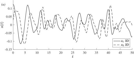
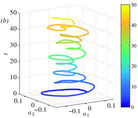
Figure 6: Time coefficients $a_{i}(t)$ of the two most energetic three-dimensional POD modes. Panel (a) shows the temporal signal, which allows to observe the qualitative quarter-period phase shift of mode 2 with respect to mode 1; panel (b) shows the (colorcoded) time over coefficients $a_{1}$ and $a_{2}$, illustrating the oscillating character. The time axis is (arbitrarily) cut at $t=50D/U_{b}$ for illustration purposes, the total recorded signal is over $300D/U_{b}$.

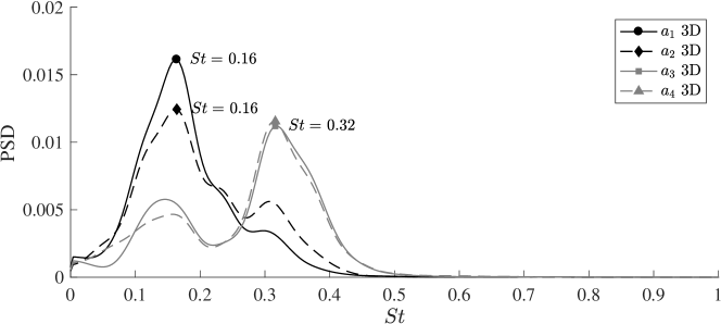
Figure 7: Welch’s power spectral density estimate for the time coefficients $a_{i}$ of the most energetic 3D POD modes. The frequencies are scaled with pipe diameter and bulk velocity. The markers and corresponding labels report the frequency corresponding to the peak of each spectrum. The range of the Strouhal number is identical to that of figure 4 to ease comparison.

The four most energetic modes are depicted in figure 5 by means of pseudocolors of normal and streamwise velocity components, as well as streamlines of the in-plane velocity. It can be observed that the modes come in pairs: 1-2 and 3-4, as is usual for POD modes and their time coefficients in a convective flow. The first coherent structure extracted by the POD is formed by modes $1$ and $2$ and constitutes a damped wave-like structure that is convected by the mean flow (see figure 5 for the spatial structure and figure 6 for the corresponding time coefficients; the supplementary video movie2_modes0-2.mov shows their behaviour in time). This is not a travelling wave such as those observed in transitional flows, as the ones of the examples mentioned in the introduction, but a coherent structure extracted by POD from a developed turbulent background that persists in fully developed turbulence, and is just a regular component of the flow on which irregular turbulent fluctuations are superimposed (see, e.g., Manhart & Wengle, 1993, for a similar case). Nevertheless, the present wave-like structure could be a surviving remnant of pre-existing, purely time-periodic, flow structures formed in the bent section and arising in the process of transition to turbulence past bends (see, e.g., the case of the flow past a circular cylinder by Sipp & Lebedev, 2007). It was found that the first instability of the flow inside of a toroidal pipe is characterised by the appearance of travelling waves (Kühnen et al., 2014; Canton et al., 2016). It is therefore possible that similar waves appear in the transition to turbulence of the present flow case, and continue to modulate the large scales of the flow at high Reynolds numbers while being submerged in small-scale turbulence. To support this hypothesis, the frequencies and wavelengths of the present coherent structures are in the same range as those measured in toroidal pipes (Canton et al., 2016), and Brücker (1998) observed swirl-switching even for $\Rey$ as low as $2\,000$, although the measured oscillations had very low amplitude.

The present modes are, obviously, not strictly periodic in space nor in time: as can be seen in figure 5(b) showing the swirl intensity, the intensity of the modes is essentially zero upstream of the bend ($s<0$), reaches a maximum at about $1D$ downstream of the bend end, and then decreases with the distance from the bend. Furthermore, the respective time coefficients are only quasiperiodic, as can be observed from their temporal signal, depicted in figure 6(a), and by their frequency spectra, figure 7(a). Nevertheless, it can be observed in figure 5 that the spatial structure of these modes is qualitatively sinusoidal along the streamwise direction $s_{o}$, with a wavelength of about $7$ pipe diameters. The figures in Brücker (1998) actually already suggest the appearance of a wave-like structure in the presence of swirl-switching.

This wave-like structure is formed by two counter-rotating swirls, visible in the 2D cross-sections in figure 5, which are advected in the streamwise direction while decaying in intensity and, at the same time, move from the inside of the bend towards the outside, as can be seen in the longitudinal cuts in figure 5 and in the supplementary video movie2_modes0-2.mov. The temporal amplitude of these modes is also qualitatively cyclic, as illustrated by the projection along the time coefficients in figure 6(b). The wave-like behaviour can be appreciated even better in the aforementioned video showing the flow reconstructed with these two modes, movie2_modes0-2.mov. Modes $1$ and $2$ are phase-shifted by a quarter of their quasi-period: figure 5 shows that the structure of mode $2$ is located approximately a quarter of a wavelength further downstream of the structure of mode $1$; while, figure 6 illustrates the constant delay of the time coefficient of mode $2$ with respect to that of mode $1$.

The second structure, formed by modes $3$ and $4$, has a spatial layout that closely resembles that of the first pair, i.e., it is also a wave-like structure, and constitutes the first “harmonic” of the wave formed by modes $1$ and $2$. The spatial structure of modes $3$ and $4$ has half of the main wavelength of modes $1$ and $2$, and the highest peak in the spectrum of the third and fourth time coefficients is at exactly twice the frequency of the peaks of $a_{1}$ and $a_{2}$, as can be seen in figure 7(a). The video movie3_modes0-4.mov shows the reconstruction of the flow field by including modes $3$ and $4$. It can be observed that these modes introduce oscillations with higher frequency and smaller amplitude when compared to the reconstruction employing only modes $1$ and $2$.

As can be observed from figure 5, the modes do not present any connection to the straight pipe section preceding the bend. This is in direct contrast with the findings of Carlsson et al. (2015), whose results were likely altered by the interference of an intrinsic frequency and wavelength on the recycling inflow boundary with the structure of the swirl-switching. Our results are, instead, in agreement with Noorani & Schlatter (2016) who observed swirl-switching in a toroidal pipe (i.e., in the absence of a straight upstream section) confirming that these large-scale oscillations are not caused by structures formed in the straight pipe, but by an effect which is intrinsic to the bent section.

The power spectral density analysis of the time coefficients of these modes, computed as a Welch’s estimate, is presented in figure 7. One can see that, unlike the PSD of the two-dimensional POD modes (figure 4), the three-dimensional modes present two distinct peaks, one per pair of modes. The peak for the first modal pair is located at $St\approx 0.16$, which is in the range of Strouhal numbers found by both Brücker (1998) and Hellström et al. (2013). More importantly, this frequency is the lowest for this pair of modes and matches that given by the wavelength and propagation speed of the wave as well as that of the swirl-switching, as observed by reconstructing the flow field with the most energetic POD modes (see the online movies).

The present analyses were also performed on a pipe with curvature $\delta=0.1$ for the same Reynolds number. Swirl-switching was observed in this case as well, with dynamics which is qualitatively identical to the one observed for $\delta=0.3$, but is characterised by lower frequencies, peaking at $St\approx 0.045$. The lower frequencies and larger scales (wavelength of about $20D$) characterising the wave-like structure at this curvature meant that a quantitative analysis was too expensive with the present setup. We have therefore limited this work to the study of one curvature only, but preliminary, not converged results can be found in Hufnagel (2016).

4 Summary and conclusions

This work presents the first DNS analysis of swirl-switching in a $90^{\circ}$ bent pipe. The simulations were performed by using a synthetic eddy method to generate high-quality inflow conditions, in an effort to avoid any interference between the incoming flow and the dynamics of the flow in the bent section, as was observed in previous studies. Three-dimensional POD was used to isolate the dominant structures of the flow. This method allowed the identification of a wave-like structure, originating in the bent section, constituted by the first modal pair. A reconstruction of the flow field using the most energetic modal pair confirmed that the swirl-switching is caused by this structure.

The swirl-switching frequency found in the present study is in the range of those deduced by Brücker (1998) and Hellström et al. (2013). The structure of the modes, which presents no connection to the upstream straight pipe, confirms what was conjectured by Noorani & Schlatter (2016), who observed swirl-switching in a toroidal pipe, namely that swirl-switching is a phenomenon intrinsic to the bent pipe section.

Clearly, the present findings are in contrast with previous conclusions drawn from flow reconstructions based on 2D POD modes and Taylor’s frozen turbulence hypothesis (see, e.g., Hellström et al., 2013): the 2D analysis mixes convection and true temporal variation, and thus cannot reveal the full three-dimensional structure of travelling modes. This does not only apply to the present flow case, but to any streamwise inhomogeneous flow in which 2D POD is utilised in the cross-flow direction.

The wave-like structure found in the present study is different from those observed in transitional flows (see, e.g. Hof et al., 2004), in the sense that it is simply a coherent structure extracted by POD from a turbulent background flow, as opposed to an exact coherent state. Nevertheless, we conjecture that this structure may be a surviving remnant of a global instability caused by the bend (Kühnen et al., 2014; Canton et al., 2016).

Financial support by the Swedish Research Council (VR) is gratefully acknowledged. Computer time was provided by the Swedish National Infrastructure for Computing (SNIC). We acknowledge that part of the results of this research have been achieved using the DECI resource SiSu based in Finland at CSC with support from the PRACE aisbl. This material is also based in part upon work supported by the US Department of Energy, office of Science, under contract DE-AC02-06CH11357.

5 Considerations on the use of 2D POD

This section explains, analytically, the reasons why a two-dimensional cross-flow POD analysis is an ineffective tool for understanding swirl-switching. In order to capture the essence of the phenomenon, the example is without spatial dissipation and noise, but these can be added at will without changing the discussion or the results. A Matlab script performing the operations described in this section is provided as part of the supplementary online material.

Consider a sine wave of period $2\pi l$, travelling at speed $v$, and with amplitude modulated at a frequency $\omega/(2\pi)$:

$$g(x,t)=\sin\left(\frac{x-vt}{l}\right)\cos\left(\omega t\right).$$ (2)

When measuring its passage at a given spatial position, say $g(x_{m},t)$, the recorded time signal will contain two frequencies, $f_{1}=(\omega-v/l)/(2\pi)$ and $f_{2}=(\omega+v/l)/(2\pi)$, that combine the spatial component, $f_{s}=v/(2\pi l)$, and the temporal component, $f_{t}=\omega/(2\pi)$. This combination is a result of the fact that $g$ can be rewritten, using one prosthaphaeresis formula, separating the time and space dependencies:

$$g(x,t)=\frac{1}{2}\sin\left[\frac{x}{l}+\left(\omega-\frac{v}{l}\right)t\right]+\frac{1}{2}\sin\left[\frac{x}{l}-\left(\omega+\frac{v}{l}\right)t\right].$$ (3)

The two components, $f_{s}$ and $f_{t}$, would be measured in isolation if the function $g$ were a pure travelling wave ($\omega=0$) or a pure standing wave ($v=0$). However, when both aspects are present ($\omega\neq 0$ and $v\neq 0$) a complete knowledge of $g$ is necessary in order to separate $f_{s}$ from $f_{t}$. This, clearly, is possible in the present example, where the analytical expression of $g(x,t)$ is known. When studying an unknown phenomenon (such as swirl-switching) the knowledge of $f_{1}$ and $f_{2}$ is insufficient: one does not know what is causing the measured frequencies: it could be two travelling waves advected at different speeds (or provided with different period); two standing waves modulated at different frequencies; or, as in this case, one travelling wave with modulated amplitude.

This problem can transferred to a POD analysis as well: the 2D POD in the pipe corresponds to a zero-dimensional POD in this example, which employs the measurements $g(x_{m},t_{i})$ as snapshots, while the 3D POD of the bent pipe flow corresponds to a one-dimensional POD which uses the function $g(x,t_{i})$ over the whole $x$ domain as snapshots.

The 0D POD returns a single mode which assumes a value of either $+1$ or $-1$ and does not provide any information about the spatial structure of $g$. The spectrum of the time coefficient corresponding to this single mode contains both frequencies $f_{1}$ and $f_{2}$. When using 0D POD one does not have any information about the spatial nature of $g$, and is lead to believe that the oscillations measured in $x_{m}$ are caused by two periodic phenomena with frequencies $f_{1}$ and $f_{2}$. This likely is what has caused so much disagreement in the literature about the value of the Strouhal number related to the swirl-switching and on the 2D POD mode responsible for this phenomenon. The answer is that none of the 2D POD modes reported in the literature is actually the swirl-switching mode, and the Strouhal numbers extracted from time coefficients do not provide a correct description.

A 1D POD analysis of the function $g$, which is the analogue of the 3D POD in the bent pipe, provides the correct answers. It results in two sinusoidal modes which, with the corresponding time coefficients, reproduce the complete travelling and oscillatory behaviour of $g$. The spectra of the time coefficients still contain only $f_{1}$ and $f_{2}$, but have a much higher peak to noise ratio compared to the 0D POD, as observed in the bent pipe by comparing figures 4 and 7. Moreover, by analysing the reconstruction of $g$, they allow the separation of $f_{s}$ from $f_{t}$.

It is now clear why in the case of a streamwise-dependent spatial structure, such as the one creating swirl-switching (as shown in §3.3), only a fully three-dimensional analysis can correctly identify the actual spatial and temporal components.

References

- Anwer et al. (1989) Anwer, M., So, R. M. C. & Lai, Y. G. 1989 Perturbation by and recovery from bend curvature of a fully developed turbulent pipe flow. Phys. Fluids 1, 1387–1397.
- Berkooz et al. (1993) Berkooz, G., Holmes, P. & Lumley, J. L. 1993 The proper orthogonal decomposition in the analysis of turbulent flows. Annu. Rev. Fluid Mech. 25, 539–575.
- Boussinesq (1868) Boussinesq, M. J. 1868 Mémoire sur l’influence des frottements dans les mouvements réguliers des fluides. J. Math. Pure Appl. 13, 377–424.
- Brücker (1998) Brücker, C. 1998 A time-recording DPIV-study of the swirl-switching effect in a bend flow. In Proc. 8th Int. Symp. Flow Vis., pp. 171.1–171.6. Sorrento (NA), Italy.
- Canton et al. (2017) Canton, J., Örlü, R. & Schlatter, P. 2017 Characterisation of the steady, laminar incompressible flow in toroidal pipes covering the entire curvature range. Int. J. Heat Fluid Flow 66, 95–107.
- Canton et al. (2016) Canton, J., Schlatter, P. & Örlü, R. 2016 Modal instability of the flow in a toroidal pipe. J. Fluid Mech. 792, 894–909.
- Carlsson et al. (2015) Carlsson, C., Alenius, E. & Fuchs, L. 2015 Swirl switching in turbulent flow through pipe bends. Phys. Fluids 27, 085112.
- Chandler & Northrop (2003) Chandler, R. & Northrop, P. 2003 Fortran random number generation. http://www.ucl.ac.uk/~ucakarc/work/randgen.html.
- Dean (1928) Dean, W. R. 1928 The streamline motion of fluid in a curved pipe. Phil. Mag. 5, 673–693.
- Doherty et al. (2007) Doherty, J., Monty, J. & Chong, M. 2007 The development of turbulent pipe flow. In 16th Australas. Fluid Mech. Conf., pp. 266–270.
- El Khoury et al. (2013) El Khoury, G. K., Schlatter, P., Noorani, A., Fischer, P. F., Brethouwer, G. & Johansson, A. V. 2013 Direct numerical simulation of turbulent pipe flow at moderately high Reynolds numbers. Flow, Turbul. Combust. 91, 475–495.
- Eustice (1910) Eustice, J. 1910 Flow of water in curved pipes. Proc. R. Soc. London, Ser. A 84, 107–118.
- Fischer et al. (2008) Fischer, P. F., Lottes, J. W. & Kerkemeier, S. G. 2008 Nek5000 Web page, http://nek5000.mcs.anl.gov.
- Hellström et al. (2013) Hellström, L. H. O., Zlatinov, M. B., Cao, G. & Smits, A. J. 2013 Turbulent pipe flow downstream of a bend. J. Fluid Mech. 735, R7.
- Hof et al. (2004) Hof, B., van Doorne, C. W. H., Westerweel, J., Nieuwstadt, F. T. M., Faisst, H., Eckhardt, B., Wedin, H., Kerswell, R. R. & Waleffe, F. 2004 Experimental observation of nonlinear traveling waves in turbulent pipe flow. Science 305, 1594–1598.
- Hufnagel (2016) Hufnagel, L. 2016 On the swirl-switching in developing bent pipe flow with direct numerical simulation. Msc thesis, KTH Mechanics, Stockholm, Sweden.
- Jarrin et al. (2006) Jarrin, N., Benhamadouche, S., Laurence, D. & Prosser, R. 2006 A synthetic-eddy-method for generating inflow conditions for large-eddy simulations. Int. J. Heat Fluid Flow 27, 585–593.
- Kalpakli & Örlü (2013) Kalpakli, A. & Örlü, R. 2013 Turbulent pipe flow downstream a pipe bend with and without superimposed swirl. Int. J. Heat Fluid Flow 41, 103–111.