Algebra, coalgebra, and minimization
in polynomial differential equations

Abstract.

We consider reasoning and minimization in systems of polynomial ordinary differential equations (ode’s). The ring of multivariate polynomials is employed as a syntax for denoting system behaviours. We endow this set with a transition system structure based on the concept of Lie derivative, thus inducing a notion of $\mathcal{L}$-bisimulation. We prove that two states (variables) are $\mathcal{L}$-bisimilar if and only if they correspond to the same solution in the ode’s system. We then characterize $\mathcal{L}$-bisimilarity algebraically, in terms of certain ideals in the polynomial ring that are invariant under Lie-derivation. This characterization allows us to develop a complete algorithm, based on building an ascending chain of ideals, for computing the largest $\mathcal{L}$-bisimulation containing all valid identities that are instances of a user-specified template. A specific largest $\mathcal{L}$-bisimulation can be used to build a reduced system of ode’s, equivalent to the original one, but minimal among all those obtainable by linear aggregation of the original equations. A computationally less demanding approximate reduction and linearization technique is also proposed.

1. Introduction

The past few years have witnessed a surge of interest in computational models based on ordinary differential equations (ode’s), ranging from continuous-time Markov chains (e.g. [4]) and process description languages oriented to bio-chemical systems (e.g. [42, 5, 13]), to deterministic approximations of stochastic systems (e.g. [18, 41]), and hybrid systems (e.g. [39, 37, 29]).

From a computational point of view, our motivation to study ode’s arises from the following problems.

1. Reasoning: provide methods to automatically prove and discover identities involving the system variables.

2. Reduction: provide methods to automatically reduce, and possibly minimize, the number of variables and equations of a system, in such a way that the reduced system retains all the relevant information of the original one.

Reasoning may help an expert (a chemist, a biologist, an engineer) to prove or to disprove certain system properties, even before actually solving, simulating or realizing the system. Often, the identities of interest take the form of conservation laws. For instance, chemical reactions often enjoy a mass conservation law, stating that the sum of the concentrations of two or more chemical species, is a constant. More generally, one would like tools to automatically discover all laws of a given form. Pragmatically, before actually solving or simulating a given system, it can be critical to reduce the system to a size that can be handled by a solver or a simulator.

Our goal is showing that these issues can be dealt with by a mix of algebraic and coalgebraic techniques. We will consider initial value problems, specified by a system of ode’s of the form $\dot{x}_{i}=f_{i}(x_{1},...,x_{N})$, for $i=1,...,N$, plus initial conditions. The functions $f_{i}$s are called drifts; here we will focus on the case where the drifts are multivariate polynomials in the variables $x_{1},..,x_{N}$. Practically, the majority of functions found in applications is in, or can be encoded into this format (possibly under restrictions on the initial conditions), including exponential, trigonometric, logarithmic and rational functions.

A more detailed account of our work follows. We introduce the ring of multivariate polynomials as a syntax for denoting the behaviours induced by the given initial value problem (Section 2). In other words, a behaviour is any polynomial combination of the individual components $x_{i}(t)$ ($i=1,..,N$) of the (unique) system solution. We then endow the polynomial ring with a transition system, based on a purely syntactic notion of Lie derivative (Section 3). This structure naturally induces a notion of bisimulation over polynomials, $\mathcal{L}$-bisimilarity, that is in agreement with the underlying ode’ s. In particular, any two variables $x_{i}$ and $x_{j}$ are $\mathcal{L}$-bisimilar if and only the corresponding solutions are the same, $x_{i}(t)=x_{j}(t)$ (this generalizes to polynomial behaviours as expected). This way, one can prove identities between two behaviours, for instance conservation laws, by exhibiting bisimulations containing the given pair . The resulting proof method is greatly enhanced by introducing a polynomial version of the up to technique of [36]. In order to turn this method into a fully automated proof procedure, we first characterize $\mathcal{L}$-bisimulation algebraically, in terms of certain ideals in the polynomial ring that are invariant under Lie-derivation (Section 4). This characterization leads to an algorithm that, given a user-specified template, returns the set of all its instances that are valid identities in the system (Section 5). One may use this algorithm, for instance, to discover all the conservation laws of the system involving terms up to a given degree. The algorithm implies building an ascending chain of ideals until stabilization, and relies on a few basic concepts from Algebraic Geometry, notably Gröbner bases [20]. The output of the algorithm is in turn essential to build a reduced system of ode’s, equivalent to the original one, but featuring a minimal number of equations and variables, in the class of systems that can be obtained by linear aggregation from the original one (Section 6). A computationally less demanding approximate reduction and linearization technique is proposed (Section 7). This may be an attractive alternative, because it is entirely based on linear algebraic, hence efficient, techniques, and produces ‘small’ linear systems. In particular, $m$ linear equations are sufficient to guarantee an approximation within $O(t^{m})$ of the original system. We then illustrate the results of some simple experiments we have conducted using a prototype implementation (in Python) of our algorithms (Section 8). Our approach is mostly related to some recent work on equivalences for ode’s by Cardelli et al. [14] and to work in the area of hybrid systems. We discuss this and other related work, as well as some possible directions for future work, in the concluding section (Section 9). In the interest of readability, some proofs and technical material have been confined to a separate appendix (Appendix A).

To sum up, we give the following contributions.

1. A complete bisimulation-based proof technique to reason on the polynomial behaviours induced by a system of ode’s.

2. An algorithm to find all the valid polynomial identities induced by the given system and fitting a user-specified template.

3. An algorithm to build a reduced, equivalent system that is minimal in the class of all linear aggregations of the original system.

4. An algorithm to build a small linear system, approximating within $O(t^{m})$ the original system.

2. Preliminaries

Let us fix an integer $N\geq 1$ and a set of $N$ distinct variables $x_{1},...,x_{N}$. We will denote by $\mathrm{\mathbf{x}}$ the column vector $(x_{1},...,x_{N})^{T}$. We let $\mathbb{R}[\mathrm{\mathbf{x}}]$ denote the set of multivariate polynomials in the variables $x_{1},...,x_{N}$ with coefficients in $\mathbb{R}$, and let $p,q$ range over it. Here we regard polynomials as syntactic objects. Given an integer $d\geq 0$, by $\mathbb{R}_{d}[\mathrm{\mathbf{x}}]$ we denote the set of polynomials of degree $\leq d$. As an example, $p=2xy^{2}+(1/5)wz+yz+1$ is a polynomial of degree $\deg(p)=3$, that is $p\in\mathbb{R}_{3}[x,y,z,w]$, with monomials $xy^{2}$, $wz$, $yz$ and 1. Depending on the context, with a slight abuse of notation it may be convenient to let a polynomial denote the induced function $\mathbb{R}^{N}\rightarrow\mathbb{R}$, defined as expected. In particular, $x_{i}$ can be seen as denoting the projection on the $i$-th coordinate.

A (polynomial) vector field is a vector of $N$ polynomials, $F=(f_{1},...,f_{N})^{T}$, seen as a function $F:\mathbb{R}^{N}\rightarrow\mathbb{R}^{N}$. A vector field $F$ and an initial condition $v_{0}\in\mathbb{R}^{N}$ together define an initial value problem $\mathbf{\Phi}=(F,v_{0})$, often written in the following form

$$\mathbf{\Phi}:\;\left\{\begin{array}[]{rcl}{\dot{\mathrm{\mathbf{x}}}(t)}&=&F(\mathrm{\mathbf{x}}(t))\\ \mathrm{\mathbf{x}}(0)&=&v_{0}\,.\end{array}\right.$$ (1)

The functions $f_{i}$ in $F$ are called drifts in this context. A solution to this problem is a differentiable function $\mathrm{\mathbf{x}}(t):D\rightarrow\mathbb{R}^{N}$, for some nonempty open interval $D\subseteq\mathbb{R}$ containing 0, which fulfills the above two equations, that is: $\frac{d}{dt}\mathrm{\mathbf{x}}(t)=F(\mathrm{\mathbf{x}}(t))$ for each $t\in D$ and $\mathrm{\mathbf{x}}(0)=v_{0}$. By the Picard-Lindelöf theorem [2], there exists a nonempty open interval $D$ containing 0, over which there is a unique solution, say $\mathrm{\mathbf{x}}(t)=(x_{1}(t),...,x_{N}(t))^{T}$, to the problem. In our case, as $F$ is infinitely often differentiable, the solution is seen to be analytic in $D$: each $x_{i}(t)$ admits a Taylor series expansion in a neighborhood of 0. For definiteness, we will take the domain of definition $D$ of $\mathrm{\mathbf{x}}(t)$ to be the largest symmetric open interval where for each $i=1,...,N$, the Taylor expansion from 0 of $x_{i}(t)$ converges pointwise to $x_{i}(t)$ (possibly $D=\mathbb{R}$). The resulting vector function of $t$, $\mathrm{\mathbf{x}}(t)$, is called the time trajectory of the system.

Given a differentiable function $g:E\rightarrow\mathbb{R}$, for some open set $E\subseteq\mathbb{R}^{N}$, the Lie derivative of $g$ along $F$ is the function $E\rightarrow\mathbb{R}$ defined as

$$\mathcal{L}_{F}(g) \stackrel{{\scriptstyle\triangle}}{{=}} \langle\nabla g,F\rangle=\sum_{i=1}^{N}(\frac{\partial g}{\partial x_{i}}\cdot f_{i})\,.$$

The Lie derivative of the sum $h+g$ and product $h\cdot g$ functions obey the familiar rules

$$\mathcal{L}_{F}(h+g) = \mathcal{L}_{F}(h)+\mathcal{L}_{F}(g)$$ (2)

$$\mathcal{L}_{F}(h\cdot g) = h\cdot\mathcal{L}_{F}(g)+\mathcal{L}_{F}(h)\cdot g\,.$$ (3)

Note that $\mathcal{L}_{F}(x_{i})=f_{i}$. Moreover if $p\in\mathbb{R}_{d}[\mathrm{\mathbf{x}}]$ then $\mathcal{L}_{F}(p)\in\mathbb{R}_{d+d^{\prime}}[\mathrm{\mathbf{x}}]$, for some integer $d^{\prime}\geq 0$ that depends on $d$ and on $F$. This allows us to view the Lie derivative of polynomials along a polynomial field $F$ as a purely syntactic mechanism, that is as a function $\mathcal{L}_{F}:\mathbb{R}[\mathrm{\mathbf{x}}]\rightarrow\mathbb{R}[\mathrm{\mathbf{x}}]$ that does not assume anything about the solution of (1). Informally, we can view $p$ as a program, and taking the Lie derivative of $p$ can be interpreted as unfolding the definitions of the variables $x_{i}$’s, according to the equations in (1) and to the formal rules for product and sum derivation, (2) and (3). We will pursue this view systematically in Section 3.

Consider $N=4$, $\mathrm{\mathbf{x}}=(x,y,z,w)^{T}$ and the set of polynomials $\mathbb{R}[\mathrm{\mathbf{x}}]$. The vector field $F=(xz+z,yw+z,z,w)^{T}$ and the initial condition $v_{0}=(0,0,1,1)^{T}$ together define an initial value problem (with no particular physical meaning) $\mathbf{\Phi}=(F,v_{0})$. This problem can be equivalently written in the form

$$\left\{\begin{array}[]{rcl}{\dot{x}(t)}&=&x(t)z(t)+z(t)\\ {\dot{y}(t)}&=&y(t)w(t)+z(t)\\ {\dot{z}(t)}&=&z(t)\\ {\dot{w}(t)}&=&w(t)\\ \mathrm{\mathbf{x}}(0)&=&v_{0}\,=\,(0,0,1,1)^{T}\,.\end{array}\right.$$ (4)

As an example of Lie derivative, if $p=2xy^{2}+wz$, we have $\mathcal{L}_{F}(p)=4wxy^{2}+2wz+2xy^{2}z+4xyz+2y^{2}z$.

The connection between time trajectories, polynomials and Lie derivatives can be summed up as follows. For any polynomial $p\in\mathbb{R}[\mathrm{\mathbf{x}}]$, the function $p\circ\mathrm{\mathbf{x}}(t):D\rightarrow\mathbb{R}$, obtained by composing $p$ as a function ${\mathbb{R}}^{N}\rightarrow{\mathbb{R}}$ with the time trajectory $\mathrm{\mathbf{x}}(t):D\rightarrow{\mathbb{R}}^{N}$, is analytic: we let $p(\mathrm{\mathbf{x}}(t))$ denote the extension of this function over the largest symmetric open interval of convergence (possibly coinciding with $\mathbb{R}$) of its Taylor expansion from 0. We will call $p(\mathrm{\mathbf{x}}(t))$ the polynomial behaviour induced by $p$ and by the initial value problem (1). The connection between Lie derivatives of $p$ along $F$ and the initial value problem (1) is given by the following equations, which can be readily checked. Here and in the sequel, we let $p(v_{0})$ denote the real number obtained by evaluating $p$ at $v_{0}$.

$$p(\mathrm{\mathbf{x}}(t))_{|t=0} = p(v_{0})$$ (5)

$$\frac{d\,}{dt}p(\mathrm{\mathbf{x}}(t)) = (\mathcal{L}_{F}(p))(\mathrm{\mathbf{x}}(t))\,.$$ (6)

More generally, defining inductively $\mathcal{L}^{(0)}_{F}(p)\stackrel{{\scriptstyle\triangle}}{{=}}p$ and $\mathcal{L}^{(j+1)}_{F}(p)\stackrel{{\scriptstyle\triangle}}{{=}}\mathcal{L}_{F}(\mathcal{L}^{j}_{F}(p))$, we have the following equation for the $j$-th derivative of $p(\mathrm{\mathbf{x}}(t))$ ($j=0,1,...$)

$$\frac{d^{j}\,}{dt^{j}}p(\mathrm{\mathbf{x}}(t)) = (\mathcal{L}^{(j)}_{F}(p))(\mathrm{\mathbf{x}}(t))\,.$$ (7)

In the sequel, we shall often abbreviate $\mathcal{L}^{(j)}_{F}(p)$ as $p^{(j)}$, and shall omit the subscript _F from $\mathcal{L}_{F}$ when clear from the context.

3. Coalgebraic semantics of polynomial ode’s

In this section we show how to endow the polynomial ring with a transition relation structure, hence giving rise to coalgebra. Bisimilarity in this coalgebra will correspond to equality between polynomial behaviours.

We recall that a (Moore) coalgebra (see e.g. [34]) with outputs in a set $O$ is a triple $C=(S,\delta,o)$ where $S$ is a set of states, $\delta:S\rightarrow S$ is a transition function, and $o:S\rightarrow O$ is an output function. A bisimulation in $C$ is a binary relation $R\subseteq S\times S$ such that whenever $s\,R\,t$ then: (a) $o(s)=o(t)$, and (b) $\delta(s)\,R\,\delta(t)$. It is an (easy) consequence of the general theory of bisimulation that a largest bisimulation over $S$, called bisimilarity and denoted by $\sim$, exists, is the union of all bisimulation relations, and is an equivalence relation over $S$.

Given an initial value problem $\mathbf{\Phi}=(F,v_{0})$ of the form (1), the triple

$$C_{\mathbf{\Phi}}\stackrel{{\scriptstyle\triangle}}{{=}}(\mathbb{R}[\mathrm{\mathbf{x}}],\mathcal{L}_{F},o)$$

forms a coalgebra with outputs in $\mathbb{R}$, where: (1) $\mathbb{R}[\mathrm{\mathbf{x}}]$ is the set of states; (2) $\mathcal{L}_{F}$ acts as the transition function; and (3) $o$ defined as $o(p)\stackrel{{\scriptstyle\triangle}}{{=}}p(v_{0})$ is the output function. Note that this definition of coalgebra is merely syntactic, and does not presuppose anything about the solution of the given initial value problem. When the standard definition of bisimulation over coalgebras is instantiated to $C_{\mathbf{\Phi}}$, it yields the following.

[$\mathcal{L}$-bisimulation $\sim_{\mathbf{\Phi}}$] Let $\mathbf{\Phi}$ be an initial value problem. A binary relation $R\subseteq\mathbb{R}[\mathrm{\mathbf{x}}]\times\mathbb{R}[\mathrm{\mathbf{x}}]$ is a $\mathcal{L}$-bisimulation if, whenever $p\,R\,q$ then: (a) $p(v_{0})=q(v_{0})$, and (b) $\mathcal{L}(p)\,R\,\mathcal{L}(q)$. The largest $\mathcal{L}$-bisimulation over $\mathbb{R}[\mathrm{\mathbf{x}}]$ is denoted by $\sim_{\mathbf{\Phi}}$.

We now introduce a new coalgebra with outputs in $\mathbb{R}$. Let $\mathcal{A}$ denote the family of real valued functions $f$ such that $f$ is analytic at 0 and $f$’s domain of definition coincides with the open interval of convergence of its Taylor series (nonempty, centered at 0, possibly coinciding with $\mathbb{R}$). We define the coalgebra of analytic functions as

$$C_{\mathrm{an}}\stackrel{{\scriptstyle\triangle}}{{=}}(\mathcal{A},(\cdot)^{\prime},o_{\mathrm{an}})$$

where $(f)^{\prime}=\frac{df}{dt}$ is the standard derivative, and $o_{\mathrm{fin}}(f)\stackrel{{\scriptstyle\triangle}}{{=}}f(0)$ is the output function. We recall that a morphism $\mu$ between two coalgebras with outputs in the same set, $\mu:C_{1}\rightarrow C_{2}$, is a function from states to states that preserves transitions ($\mu(\delta_{1}(s))=\delta_{2}(\mu(s))$) and outputs ($o_{1}(s)=o_{2}(\mu(s))$). It is a standard (and easy) result of coalgebra that a morphism maps bisimilar states into bisimilar states: $s\sim_{1}s^{\prime}$ implies $\mu(s)\sim_{2}\mu(s^{\prime})$.

The coalgebra $C_{\mathrm{an}}$ has a special status, in that, given any coalgebra $C$ with outputs in $\mathbb{R}$, if there is a morphism from $C$ to $C_{\mathrm{an}}$, this morphism is guaranteed to be unique. For our purposes, it is enough to focus on $C=C_{\mathbf{\Phi}}$. We define the function $\mu:\mathbb{R}[\mathrm{\mathbf{x}}]\rightarrow\mathcal{A}$ as

$$\mu(p) \stackrel{{\scriptstyle\triangle}}{{=}} p(\mathrm{\mathbf{x}}(t))\,.$$

Theorem 1 (coinduction).

$\mu$ is the unique morphism from $C_{\mathbf{\Phi}}$ to $C_{\mathrm{an}}$. Moreover, the following coinduction principle is valid: $p\sim_{\mathbf{\Phi}}q$ in $C_{\mathbf{\Phi}}$ if and only if $p(\mathrm{\mathbf{x}}(t))=q(\mathrm{\mathbf{x}}(t))$ in $\mathcal{A}$.

Proof 3.1.

The function $\mu$ given above is well defined, because $p(\mathrm{\mathbf{x}}(t))\in\mathcal{A}$, and is a morphism: for output and transition preservation, use (5) and (6), respectively. By the above recalled standard result in coalgebra, then $p\sim_{\mathbf{\Phi}}q$ implies $p(\mathrm{\mathbf{x}}(t))\sim q(\mathrm{\mathbf{x}}(t))$ in $C_{\mathrm{an}}$. Assume now that $\nu$ is a morphism from $C_{\mathbf{\Phi}}$ to $C_{\mathrm{an}}$. From the definition of morphism and bisimulation, it is readily checked that for each $p$, $\mu(p)\sim\nu(p)$ in $C_{\mathrm{an}}$. Finally, we check that $\sim$ in $C_{\mathrm{an}}$ coincides with equality: indeed, if two functions are bisimilar in $\mathcal{A}$, then they have the same Taylor coefficients (this is shown by induction on the order of the derivatives, relying on the fact that $f\sim g$ means $f(0)=g(0)$ and $f^{\prime}\sim g^{\prime}$); the vice-versa is obvious. This completes the proof of both parts of the statement.

Remark 2 (categorical presentation).

Existence of a morphism from any coalgebra with outputs in ${\mathbb{R}}$ into $C_{\mathrm{an}}$ is not guaranteed: for instance, the sequence (stream) of coefficients of any series with a radius of convergence 0, such as $(0!,1!,2!,...,i!,...)$, trivially induces a coalgebra from which no morphism to $C_{\mathrm{an}}$ exists. In this sense, $C_{\mathrm{an}}$ is not final. Note that $C_{\mathrm{an}}$ can be injected into the coalgebra of streams in the sense of Rutten [34], which is indeed final.

In a more categorical perspective, $C_{\mathrm{an}}$ induces a so-called covariety – see e.g. [22] – that is, the category of coalgebras that have a unique morphism into $C_{\mathrm{an}}$: $C_{\mathrm{an}}$ is of course final in this covariety. How to characterise such covariety more explicitly, for example in terms of comonads, is left for future research.

Theorem 1 allows one to prove polynomial relations among the components $x_{i}(t)$ of $\mathrm{\mathbf{x}}(t)$, say that $p(\mathrm{\mathbf{x}}(t))=q(\mathrm{\mathbf{x}}(t))$, by coinduction, that is, by exhibiting a suitable $\mathcal{L}$-bisimulation relating the polynomials $p$ and $q$.

For $N=2$, consider the vector field $F=(x_{2},-x_{1})^{T}$ with the initial value $v_{0}=(0,1)^{T}$. The binary relation $R\subseteq\mathbb{R}[x_{1},x_{2}]\times\mathbb{R}[x_{1},x_{2}]$ defined thus

$$R=\{\,(0,0),\,(x_{1}^{2}+x_{2}^{2},1)\,\}$$

is easily checked to be an $\mathcal{L}$-bisimulation. Thus we have proved the polynomial relation $x_{1}^{2}(t)+x_{2}^{2}(t)=1$. Note that the unique solution to the given initial value problem is the pair of functions $\mathrm{\mathbf{x}}(t)=(\sin(t),\cos(t))^{T}$. This way we have proven the familiar trigonometric identity $\sin(t)^{2}+\cos(t)^{2}=1$.

This proof method can be greatly enhanced by a so called $\mathcal{L}$-bisimulation up to technique, in the spirit of [36]. This can be regarded as a form of up-to context technique, since we are just considering the closure w.r.t. the syntax, that is, the algebraic structure of the polynomial ring.

[$\mathcal{L}$-bisimulation up to] Let $R\subseteq\mathbb{R}[\mathrm{\mathbf{x}}]\times\mathbb{R}[\mathrm{\mathbf{x}}]$ be a binary relation. Consider the binary relation $\widehat{R}$ defined by: $p\,\widehat{R}\,q$ iff there are $m\geq 0$ and polynomials $h_{i},p_{i},q_{i}$ ($i=1,...,m$) such that: $p=\sum_{i=1}^{m}h_{i}p_{i}$ and $q=\sum_{i=1}^{m}h_{i}q_{i}$ and $p_{i}\,R\,q_{i}$, for $i=1,...,m$.

A relation $R\subseteq\mathbb{R}[\mathrm{\mathbf{x}}]\times\mathbb{R}[\mathrm{\mathbf{x}}]$ is a $\mathcal{L}$-bisimulation up to if, whenever $p\,R\,q$ then: (a) $p(v_{0})=q(v_{0})$, and (b) $\mathcal{L}(p)\,\widehat{R}\,\mathcal{L}(q)$.

Note that, from the definition, for each relation $R$ we have $R\subseteq\widehat{R}$.

Lemma 3.

Let $R$ be an $\mathcal{L}$-bisimulation up to. Then $\widehat{R}$ is an $\mathcal{L}$-bisimulation, consequently $R\,\subseteq\,\sim_{\mathbf{\Phi}}$.

Proof 3.2.

In order to check that $\widehat{R}$ is an $\mathcal{L}$-bisimulation, assume that $p\,\widehat{R}\,q$, that is $p=\sum_{i=1}^{m}h_{i}p_{i}$ and $q=\sum_{i=1}^{m}h_{i}q_{i}$, for some $h_{i},p_{i},q_{i}$ ($i=1,...,m$) as specified by Definition 2. It is immediate to check that $p(v_{0})=q(v_{0})$, which proves condition (a) of the definition of $\mathcal{L}$-bisimulation. Furthermore, for each $i=1,..,m$, we have by assumption that $\mathcal{L}(p_{i})\,\widehat{R}\,\mathcal{L}(q_{i})$. That is, for suitable $g_{ij}$’s and $r_{ij}$’s, we have

$$\mathcal{L}(p_{i}) =\sum_{j}g_{ij}r_{ij} \mathcal{L}(q_{i}) =\sum_{j}g_{ij}s_{ij} r_{ij}\, R\,s_{ij}\,.$$

Recalling the rules for the Lie derivative, (2) and (3), we have

$$\mathcal{L}(p) =\;\sum_{i}h_{i}\mathcal{L}(p_{i})+\mathcal{L}(h_{i})p_{i} =\sum_{i}h_{i}\sum_{j}g_{ij}r_{ij}+\mathcal{L}(h_{i})p_{i} =\sum_{i}\sum_{j}h_{i}g_{ij}r_{ij}+\sum_{i}\mathcal{L}(h_{i})p_{i}$$

$$\widehat{R}\;\sum_{i}\sum_{j}h_{i}g_{ij}s_{ij}+\sum_{i}\mathcal{L}(h_{i})q_{i} =\sum_{i}h_{i}\sum_{j}g_{ij}s_{ij}+\sum_{i}\mathcal{L}(h_{i})q_{i} =\sum_{i}h_{i}\mathcal{L}(q_{i})+\mathcal{L}(h_{i})q_{i}\hskip 31.2982pt$$

$$=\;\mathcal{L}(q)\mbox{\ }\,.$$

This proves condition (b) of the definition of $\mathcal{L}$-bisimulation.

Consider the initial value problem of Example 2 and the relation defined below

$$R\;=\;\{\,(xz^{j},yw^{j})\,,\,(z^{j},w^{j})\,:\,j\geq 0\}\,.$$

It is easy to check that $R$ is an $\mathcal{L}$-bisimulation up to. As an example, let us check condition (b) for a pair $(xz^{j},yw^{j})$:

$$\mathcal{L}(xz^{j})\,=\,(xz+z)z^{j}+jxz^{j}\,=\,(xz^{j+1}+jxz^{j}+zz^{j})\;\widehat{R}\;(yw^{j+1}+jyw^{j}+zw^{j})\,=\,(yw+z)w^{j}+jyw^{j}\,=\,\mathcal{L}(yw^{j})\,.$$

This proves that $x(t)=y(t)$ and that $z(t)=w(t)$. In the next two sections we will prove that this technique can be fully automated by resorting to the concept of ideal in a polynomial ring.

4. Algebraic characterization of $\mathcal{L}$-bisimilarity

We first review the notion of polynomial ideal from Algebraic Geometry, referring the reader to e.g. [20] for a comprehensive treatment. A set of polynomials $I\subseteq\mathbb{R}[\mathrm{\mathbf{x}}]$ is an ideal if: (1) $0\in I$, (2) $I$ is closed under sum +, (3) $I$ is absorbing under product $\cdot$, that is $p\in I$ implies $h\cdot p\in I$ for each $h\in\mathbb{R}[\mathrm{\mathbf{x}}]$. Given a set of polynomials $S$, the ideal generated by $S$, denoted by $\big{\langle}\,\,S\,\,\big{\rangle}$, is defined as

$$\left\{\sum_{j=1}^{m}h_{j}p_{j}\,:\,\text{ $m\geq 0$, $h_{j}\in\mathbb{R}[\mathrm{\mathbf{x}}]$ and $p_{j}\in S$, for }j=1,...,m\right\}\,.$$ (8)

The polynomial coefficients $h_{j}$ in the above definition are called multipliers. It is clear that $\big{\langle}\,\,S\,\,\big{\rangle}$ is the smallest ideal containing $S$, which implies that $\big{\langle}\,\,\big{\langle}\,\,S\,\,\big{\rangle}\,\,\big{\rangle}=\big{\langle}\,\,S\,\,\big{\rangle}$. Any set $S$ such that $\big{\langle}\,\,S\,\,\big{\rangle}=I$ is called a basis of $I$. Every ideal in the polynomial ring $\mathbb{R}[\mathrm{\mathbf{x}}]$ is finitely generated, that is has a finite basis (a version of Hilbert’s basis theorem).

$\mathcal{L}$-bisimulations can be connected to certain types of ideals. This connection relies on Lie derivatives. First, we define the Lie derivative of any set $S\subseteq\mathbb{R}[\mathrm{\mathbf{x}}]$ as follows

$$\mathcal{L}(S) \stackrel{{\scriptstyle\triangle}}{{=}} \{\mathcal{L}(p):p\in S\}\,.$$

We say that $S$ is a pre-fixpoint of $\mathcal{L}$ if $\mathcal{L}(S)\subseteq S$. $\mathcal{L}$-bisimulations can be characterized as particular pre-fixpoints of $\mathcal{L}$ that are also ideals, called invariants.

[invariant ideals] Let $\mathbf{\Phi}=(F,v_{0})$. An ideal $I$ is a $\mathbf{\Phi}$-invariant if: (a) $p(v_{0})=0$ for each $p\in I$, and (b) $I$ is a pre-fixpoint of $\mathcal{L}_{F}$.

We will drop the $\mathbf{\Phi}$- from $\mathbf{\Phi}$-invariant whenever this is clear from the context. The following definition and lemma provide the link between invariants and $\mathcal{L}$-bisimulation.

[kernel] The kernel of a binary relation $R\subseteq{\mathbb{R}}[\mathrm{\mathbf{x}}]\times{\mathbb{R}}[\mathrm{\mathbf{x}}]$ is $\ker(R)\stackrel{{\scriptstyle\triangle}}{{=}}\{p-q:p\,R\,q\}$.

Lemma 4.

Let $R$ be a binary relation. If $R$ is an $\mathcal{L}$-bisimulation then $\big{\langle}\,\,\ker(R)\,\,\big{\rangle}$ is an invariant. Conversely, given an invariant $I$, then $R=\{(p,q):p-q\in I\}$ is an $\mathcal{L}$-bisimulation.

Consequently, proving that $p\sim_{\mathbf{\Phi}}q$ is equivalent to exhibiting an invariant $I$ such that $p-q\in I$.

Consider the initial value problem of Example 3. Let $I=\big{\langle}\,\,\{x-y,z-w\}\,\,\big{\rangle}$. Let us check that $I$ is an invariant. Let $p=h_{1}(x-y)+h_{2}(z-w)$ be a generic element of $I$. Clearly $p(v_{0})=0$, thus condition (a) is satisfied. Concerning (b), we consider the two summands separately:

$$\mathcal{L}(h_{1}(x-y)) = \mathcal{L}(h_{1})(x-y)+h_{1}\mathcal{L}(x-y)$$

$$= \mathcal{L}(h_{1})(x-y)+h_{1}(xz+z-(yz+w))$$

$$= \big{(}\mathcal{L}(h_{1})+h_{1}z\big{)}(x-y)+h_{1}(z-w)$$

$$\in I$$

$$\mathcal{L}(h_{2}(z-w)) = \mathcal{L}(h_{1})(z-w)+h_{1}\mathcal{L}(z-w)$$

$$= \mathcal{L}(h_{1})(z-w)+h_{1}(z-w)$$

$$= \big{(}\mathcal{L}(h_{1})+h_{1}\big{)}(z-w)$$

$$\in I\,.$$

Consequently, $\mathcal{L}(p)=\mathcal{L}(h_{1}(x-y))+\mathcal{L}(h_{2}(z-w))\in I$.

A more general problem than equivalence checking is finding all valid polynomial equations of a given form. We will illustrate an algorithm to this purpose in the next section.

The following result sums up the different characterization of $\mathcal{L}$-bisimilarity $\sim_{\mathbf{\Phi}}$. In what follows, we will denote the constant zero function in $\mathcal{A}$ simply by $0$ and consider the following set of polynomials.

$$\mathcal{Z}_{\mathbf{\Phi}} \stackrel{{\scriptstyle\triangle}}{{=}} \{p:p(\mathrm{\mathbf{x}}(t))\mbox{ is identically }0\,\}\,.$$

The following result also proves that $\mathcal{Z}_{\mathbf{\Phi}}$ is the largest $\mathbf{\Phi}$-invariant.

Theorem 5 ($\mathcal{L}$-bisimilarity via ideals).

We have the following characterizations of $\mathcal{L}$-bisimilarity. For any pair of polynomials $p$ and $q$:

$$p\,\sim_{\mathbf{\Phi}}\,q\;\text{ iff }\;p-q \in \ker(\sim_{\mathbf{\Phi}})$$ (9)

$$= \mathcal{Z}_{\mathbf{\Phi}}$$ (10)

$$= \left\{p:\,p^{(j)}(v_{0})=0\text{ for each }j\geq 0\right\}$$ (11)

$$= \bigcup\left\{I:\,I\text{ is a $\mathbf{\Phi}$-invariant }\right\}\,.$$ (12)

5. Computing invariants

By Theorem 5, proving $p\sim_{\mathbf{\Phi}}q$ means finding an invariant $I$ such that $p-q\in I\subseteq\mathcal{Z}_{\mathbf{\Phi}}$. More generally, we focus here on the problem of finding invariants that include a user-specified set of polynomials. In the sequel, we will make use of the following two basic facts about ideals, for whose proof we refer the reader to [20].

1. Any infinite ascending chain of ideals in a polynomial ring, $I_{0}\subseteq I_{1}\subseteq\cdots$, stabilizes at some finite $k$. That is, there is $k\geq 0$ such that $I_{k}=I_{k+j}$ for each $j\geq 0$. This is just another version of Hilbert’s basis theorem.

2. The ideal membership problem, that is, deciding whether $p\in I$, given $p$ and a finite set of $S$ of generators (such that $I=\big{\langle}\,\,S\,\,\big{\rangle}$), is decidable (provided the coefficients used in $p$ and in $S$ can be finitely represented), although it requires exponential space in the number of variables. The ideal membership will be further discussed later on in the section.

The main idea is introduced by the naive algorithm presented below.

5.1. A naive algorithm

Suppose we want to decide whether $p\in\mathcal{Z}_{\mathbf{\Phi}}$. It is quite easy to devise an algorithm that computes the smallest invariant containing $p$, or returns ‘no’ in case no such invariant exists, i.e. in case $p\notin\mathcal{Z}_{\mathbf{\Phi}}$. Consider the successive Lie derivatives of $p$, $p^{(j)}=\mathcal{L}^{(j)}(p)$ for $j=0,1,...$. For each $j\geq 0$, let $I_{j}\stackrel{{\scriptstyle\triangle}}{{=}}\big{\langle}\,\,\{p^{(0)},...,p^{(j)}\}\,\,\big{\rangle}$. Let $m$ be the least integer such that either

• $p^{(m)}(v_{0})\neq 0$, or

• $I_{m}=I_{m+1}$.

If (a) occurs, then $p\notin\mathcal{Z}_{\mathbf{\Phi}}$, so we return ‘no’ (Theorem 5(11)); if (b) occurs, then $I_{m}$ is the least invariant containing $p$. Note that the integer $m$ is well defined: $I_{0}\subseteq I_{1}\subseteq I_{2}\subseteq\cdots$ forms an infinite ascending chain of ideals, which must stabilize in a finite number of steps (fact 1 at the beginning of the section). In particular, as soon as $I_{i+1}=I_{i}$ the chain gets stable, as a consequence of the derivation rules (2) and (3).

Checking condition (b) amounts to deciding if $p^{(m+1)}\in I_{m}$. This is an instance of the ideal membership problem, which can be solved effectively. Generally speaking, given a polynomial $p$ and finite set of polynomials $S$, deciding the ideal membership $p\in I=\big{\langle}\,\,S\,\,\big{\rangle}$ can be accomplished by first transforming $S$ into a Gröbner basis $G$ for $I$ (via, e.g. the Buchberger’s algorithm), then computing $r$, the residual of $p$ modulo $G$ (via a sort generalised division of $p$ by $G$): one has that $p\in I$ if and only if $r=0$ (again, this procedure can be carried out effectively only if the coefficients involved in $p$ and $S$ are finitely representable; in practice, one often confines to rational coefficients). We refer the reader to [20] for further details on the ideal membership problem. Known procedures to compute Gröbner bases have exponential worst-case space complexity depending on the number of variables, although may perform reasonably well in some concrete cases. One should in any case invoke such procedures parsimoniously. Here is a small example to illustrate the above outlined algorithm.

Consider again the initial value problem of Example 3. Let $p=x-y$. With the help of a computer algebra system, we can easily check the following.

• $p^{(0)}=p$ and $p^{(0)}(v_{0})=0$;

• $p^{(1)}=xz-yw$, $p^{(1)}(v_{0})=0$ and $p^{(1)}\notin I_{0}=\big{\langle}\,\,\{p^{(0)}\}\,\,\big{\rangle}$;

• $p^{(2)}=-w^{2}y-wy-wz+xz^{2}+xz+z^{2}$, $p^{(2)}(v_{0})=0$ and $p^{(2)}\notin I_{1}=\big{\langle}\,\,\{p^{(0)},p^{(1)}\}\,\,\big{\rangle}$

• $p^{(3)}=-w^{3}y-3w^{2}y-w^{2}z-wy-3wz+xz^{3}+3xz^{2}+xz+z^{3}+3z^{2}$, $p^{(3)}(v_{0})=0$ and finally $p^{(3)}\in I_{2}=\big{\langle}\,\,\{p^{(0)},p^{(1)},p^{(2)}\}\,\,\big{\rangle}$.

Hence $I_{2}$ is the least invariant containing $p=x-y$, thus proving that $x-y\in\mathcal{Z}_{\mathbf{\Phi}}$.

We will introduce below a more general algorithm, which can also deal with (infinite) sets of user-specified polynomials. First, we need to introduce the concept of template.

5.2. Templates

Polynomial templates have been introduced by Sankaranarayanan, Sipma and Manna in [37] as a means to compactly specify sets of polynomials. Fix a tuple of $n\geq 1$ of distinct parameters, say $\mathrm{\mathbf{a}}=(a_{1},...,a_{n})$, disjoint from $\mathrm{\mathbf{x}}$. Let $Lin(\mathrm{\mathbf{a}})$, ranged over by $\ell$, be the set of linear expressions with coefficients in $\mathbb{R}$ and variables in $\mathrm{\mathbf{a}}$; e.g. $\ell=5a_{1}+42a_{2}-3a_{3}$ is one such expression. A template is a polynomial in $Lin(\mathrm{\mathbf{a}})[\mathrm{\mathbf{x}}]$, that is, a polynomial with linear expressions as coefficients; we let $\pi$ range over templates. For example, the following is a template:

$$\pi = (5a_{1}+(3/4)a_{3})xy^{2}+(7a_{1}+(1/5)a_{2})xz+(a_{2}+42a_{3})\,.$$

Given a vector $v=(\lambda_{1},...,\lambda_{n})^{T}\in\mathbb{R}^{n}$, we will let $\ell[v]\in\mathbb{R}$ denote the result of replacing each parameter $a_{i}$ with $\lambda_{i}$, and evaluating the resulting expression; we will let $\pi[v]\in\mathbb{R}[\mathrm{\mathbf{x}}]$ denote the polynomial obtained by replacing each $\ell$ with $\ell[v]$ in $\pi$. Given a set $S\subseteq\mathbb{R}^{n}$, we let $\pi[S]$ denote the set $\{\pi[v]\,:\,v\in S\}\subseteq\mathbb{R}[\mathrm{\mathbf{x}}]$.

The (formal) Lie derivative of $\pi$ is defined as expected, once linear expressions are treated as constants; note that $\mathcal{L}(\pi)$ is still a template. It is easy to see that the following property is true: for each $\pi$ and $v$, one has $\mathcal{L}(\pi[v])=\mathcal{L}(\pi)[v]$. This property extends as expected to the $j$-th Lie derivative ($j\geq 0$)

$$\mathcal{L}^{(j)}(\pi[v]) = \mathcal{L}^{(j)}(\pi)[v]\,.$$ (13)

5.3. A double chain algorithm

We present an algorithm that, given a template $\pi$ with $n$ parameters, returns a pair $(V,J)$, where $V\subseteq\mathbb{R}^{n}$ is such that $\pi[\mathbb{R}^{n}]\cap\mathcal{Z}_{\mathbf{\Phi}}=\pi[V]$, and $J$ is the smallest invariant that includes $\pi[V]$. We first give a purely mathematical description of the algorithm, postponing its effective representation to the next subsection. The algorithm is based on building two chains of sets, a descending chain of vector spaces and an (eventually) ascending chain of ideals. The ideal chain is used to detect the stabilization of the sequence. In fact, in the sequence of vector spaces below, $V_{i+1}=V_{i}$ does not in itself imply that $V_{i+k}=V_{i}$ for each $k\geq 1$. Formally, for each $i\geq 0$, consider the sets

$$V_{i} \stackrel{{\scriptstyle\triangle}}{{=}} \{v\in\mathbb{R}^{n}\,:\,\pi^{(j)}[v](v_{0})=0\text{ for }j=0,...,i\,\}$$ (14)

$$J_{i} \stackrel{{\scriptstyle\triangle}}{{=}} \big{\langle}\,\,\bigcup_{j=0}^{i}\pi^{(j)}[V_{i}]\,\,\big{\rangle}\,.$$ (15)

It is easy to check that each $V_{i}\subseteq\mathbb{R}^{n}$ is a vector space over $\mathbb{R}$ of dimension $\leq n$. Now let $m\geq 0$ be the least integer such that the following conditions are both true:

$$V_{m+1} = V_{m}$$ (16)

$$J_{m+1} = J_{m}\,.$$ (17)

The algorithm returns $(V_{m},J_{m})$. Note that the integer $m$ is well defined: indeed, $V_{0}\supseteq V_{1}\supseteq\cdots$ forms an infinite descending chain of finite-dimensional vector spaces, which must stabilize in finitely many steps. In other words, we can consider the least $m^{\prime}$ such that $V_{m^{\prime}}=V_{m^{\prime}+k}$ for each $k\geq 1$. Then $J_{m^{\prime}}\subseteq J_{m^{\prime}+1}\subseteq\cdots$ forms an infinite ascending chain of ideals, which must stabilize at some $m\geq m^{\prime}$. Therefore there must be some index $m$ such that (16) and (17) are both satisfied, and we choose the least such $m$.

The next theorem states the correctness and relative completeness of this abstract algorithm. Informally, the algorithm will output the largest space $V_{m}$ such that $\pi[V_{m}]\subseteq\mathcal{Z}_{\mathbf{\Phi}}$ and the smallest invariant $J_{m}$ witnessing this inclusion. Note that, while typically the user will be interested in $\pi[V_{m}]$, $J_{m}$ as well may contain useful information, such as higher order, nonlinear conservation laws. We need a technical lemma.

Lemma 6.

Let $V_{m},J_{m}$ be the sets returned by the algorithm. Then for each $j\geq 1$, one has $V_{m}=V_{m+j}$ and $J_{m}=J_{m+j}$.

Theorem 7 (correctness and relative completeness).

Let $V_{m},J_{m}$ be the sets returned by the algorithm for a polynomial template $\pi$.

• $\pi[V_{m}]=\mathcal{Z}_{\mathbf{\Phi}}\cap\pi[\mathbb{R}^{n}]$;

• $J_{m}$ is the smallest invariant containing $\pi[V_{m}]$.

Proof 5.1.

Concerning part (a), we first note that $\pi[v]\in\mathcal{Z}_{\mathbf{\Phi}}\cap\pi[\mathbb{R}^{n}]$ means $(\pi[v])^{(j)}(v_{0})=\pi^{(j)}[v](v_{0})=0$ for each $j\geq 0$ (Theorem 5(11)), which, by definition, implies $v\in V_{j}$ for each $j\geq 0$, hence $v\in V_{m}$. Conversely, if $v\in V_{m}=V_{m+1}=V_{m+2}=\cdots$ (here we are using Lemma 6), then by definition $(\pi[v])^{(j)}(v_{0})=\pi^{(j)}[v](v_{0})=0$ for each $j\geq 0$, which implies that $\pi[v]\in\mathcal{Z}_{\mathbf{\Phi}}$ (again Theorem 5(11)). Note that in proving both inclusions we have used property (13).

Concerning part (b), it is enough to prove that: (1) $J_{m}$ is an invariant, (2) $J_{m}\supseteq\mathcal{Z}_{\mathbf{\Phi}}\cap\pi[\mathbb{R}^{n}]$, and (3) for any invariant $I$ such that $\mathcal{Z}_{\mathbf{\Phi}}\cap\pi[\mathbb{R}^{n}]\subseteq I$, we have that $J_{m}\subseteq I$. We first prove (1), that $J_{m}$ is an invariant. Indeed, for each $v\in V_{m}$ and each $j=0,...,m-1$, we have $\mathcal{L}(\pi^{(j)}[v])=\pi^{(j+1)}[v]\in J_{m}$ by definition, while for $j=m$, since $v\in V_{m}=V_{m+1}$, we have $\mathcal{L}(\pi^{(m)}[v])=\pi^{(m+1)}[v]\in J_{m+1}=J_{m}$ (note that in both cases we have used property (13)). Concerning (2), note that $J_{m}\supseteq\pi[V_{m}]=\mathcal{Z}_{\mathbf{\Phi}}\cap\pi[\mathbb{R}^{n}]$ by virtue of part (a). Concerning (3), consider any invariant $I\supseteq\mathcal{Z}_{\mathbf{\Phi}}\cap\pi[\mathbb{R}^{n}]$. We show by induction on $j=0,1,...$ that for each $v\in V_{m}$, $\pi^{(j)}[v]\in I$; this will imply the wanted statement. Indeed, $\pi^{(0)}[v]=\pi[v]\in\mathcal{Z}_{\mathbf{\Phi}}\cap\pi[\mathbb{R}^{n}]$, as $\pi[V_{m}]\subseteq\mathcal{Z}_{\mathbf{\Phi}}$ by (a). Assuming now that $\pi^{(j)}[v]\in I$, by invariance of $I$ we have $\pi^{(j+1)}[v]=\mathcal{L}(\pi^{(j)}[v])\in I$ (again, we have used here property (13)).

According to Theorem 7(a), given a template $\pi$ and $v\in\mathbb{R}^{n}$, checking if $\pi[v]\in\pi[V_{m}]$ is equivalent to checking if $v\in V_{m}$, which can be effectively done knowing a basis $B_{m}$ of $V_{m}$. We show how to effectively compute such a basis in the following.

5.4. Effective representation

For $i=0,1,...$, we have to give effective ways to:

1. represent the sets $V_{i},J_{i}$ in (14) and (15); and

2. check the termination conditions (16) and (17).

It is quite easy to address (i) and (ii) in the case of the vector spaces $V_{i}$. For each $i$, consider the linear expression $\pi^{(i)}(v_{0})$. By factoring out the parameters $a_{1},...,a_{n}$ in this expression, we can write, for a suitable (row) vector of coefficients $t_{i}=(t_{i1},...,t_{in})\in\mathbb{R}^{1\times n}$:

$$\pi^{(i)}(v_{0}) = t_{i1}\cdot a_{1}+\cdots+t_{in}\cdot a_{n}$$

The condition on $v\in\mathbb{R}^{n}$, $\pi^{(i)}[v](v_{0})=0$, can then be translated into the linear constraint on $v$

$$t_{i}\cdot v = 0\,.$$ (18)

Letting $T_{i}\in\mathbb{R}^{i\times n}$ denote the matrix obtained by stacking the rows $t_{1},...,t_{i}$ on above the other, we see that $V_{i}$ is the right null space of $T_{i}$. That is (here, $\mathbf{0}_{i}$ denotes the null vector in $\mathbb{R}^{i}$):

$$V_{i} = \{v\in\mathbb{R}^{n}\,:\,T_{i}v=\mathbf{0}_{i}\,\}\,.$$

Checking whether $V_{i}=V_{i+1}$ or not amounts then to checking whether the vector $t_{i+1}$ is or not linearly dependent from the rows in $T_{i}$, which can be accomplished by standard and efficient linear algebraic techniques. In practice, the linear constraints (18) can be resolved and propagated incrementally, as they are generated, following the computation of the derivatives $\pi^{(i)}$. Concerning the representation of the ideals $J_{i}$, we will use the following lemma.

Lemma 8.

Let $V\subseteq\mathbb{R}^{n}$ be a vector space with $B$ as a basis, and $\pi_{1},...,\pi_{k}$ be templates. Then $\big{\langle}\,\,\cup_{j=0}^{k}\pi_{j}[V]\,\,\big{\rangle}=\big{\langle}\,\,\cup_{j=0}^{k}\pi_{j}[B]\,\,\big{\rangle}$.

Now let $B_{i}$ be a finite basis of $V_{i}$, which can be easily built from the matrix $T_{i}$. By the previous lemma, $\cup_{j=1}^{i}\pi^{(j)}[B_{i}]$ is a finite set of generators for $J_{i}$: this solves the representation problem. Concerning the termination condition, we note that, after checking that actually $V_{i}=V_{i+1}$, checking $J_{i}=J_{i+1}$ reduces to checking that

$$\pi^{(i+1)}[B_{i}] \subseteq \big{\langle}\,\,\cup_{j=0}^{i}\pi^{(j)}[B_{i}]\,\,\big{\rangle}\;=\;J_{i}\,.$$ (19)

To check this inclusion, one can apply standard computer algebra techniques. For example, one can check if $\pi^{(i+1)}[b]\in J_{i}$ for each $b\in B_{i}$, thus solving $|B_{i}|$ ideal membership problems, for one and the same ideal $J_{i}$. As already discussed, this presupposes the computation of a Gröbner basis for $J_{i}$, a potentially expensive operation. One advantage of the above algorithm, over methods proposed in program analysis with termination conditions based on testing ideal membership (e.g. [32]), is that (19) is not checked at every iteration, but only when $V_{i+1}=V_{i}$ (the latter a relatively inexpensive check). In the Appendix (Subsection A.2), we also discuss a sufficient condition which does not involve Gröbner bases, but leads to an incomplete algorithm.

Consider the initial value problem of Example 2 and the template $\pi=a_{1}x+a_{2}y+a_{3}z+a_{4}w$. We run the double chain algorithm with this system and template as inputs. In what follows, $v=(v_{1},v_{2},v_{3},v_{4})^{T}$ will denote a generic vector in $\mathbb{R}^{4}$. Recall that $\mathrm{\mathbf{x}}=(x,y,z,w)^{T}$ and $v_{0}=(0,0,1,1)^{T}$.

• For each $v\in\mathbb{R}^{4}$: $\pi^{(0)}[v](v_{0})=(v_{1}x+v_{2}y+v_{3}z+v_{4}w)(v_{0})=0$ if and only if $v\in V_{0}\stackrel{{\scriptstyle\triangle}}{{=}}\{v\,:\,v_{3}=-v_{4}\}$.

• For each $v\in V_{0}$: $\pi^{(1)}[v](v_{0})=(v_{1}xz+v_{1}z+v_{2}wy+v_{2}z+v_{4}w-v_{4}z)(v_{0})=0$ if and only if $v\in V_{1}\stackrel{{\scriptstyle\triangle}}{{=}}\{v\in V_{0}:v_{1}=-v_{2}\}$.

• For each $v\in V_{1}$: $\pi^{(2)}[v](v_{0})=(v_{2}w^{2}y+v_{2}wy+v_{2}wz-v_{2}xz^{2}-v_{2}xz-v_{2}z^{2}+v_{4}w-v_{4}z)(v_{0})=0$ if and only if $v\in V_{2}\stackrel{{\scriptstyle\triangle}}{{=}}V_{1}$.
  Being $V_{2}=V_{1}$, we also check if $J_{2}=J_{1}$. A basis of $V_{1}$ is $B_{1}=\{b_{1},b_{2}\}$ with $b_{1}=(-1,1,0,0)^{T}$ and $b_{2}=(0,0,-1,1)^{T}$. According to (19), we have therefore to check if, for $\ell=1,2$:

  $$\pi^{(2)}[b_{\ell}] \in J_{1}\stackrel{{\scriptstyle\triangle}}{{=}}\big{\langle}\,\,\{\pi^{(0)}[b_{1}],\pi^{(0)}[b_{2}],\pi^{(1)}[b_{1}],\pi^{(1)}[b_{2}]\}\,\,\big{\rangle}\,.$$

  With the help of a computer algebra system, one computes a Gröbner basis for $J_{1}$ as $G_{1}=\{x-y,z-w\}$. Then one can reduce $\pi^{(2)}[b_{1}]=w^{2}y+wy+wz-xz^{2}-xz-z^{2}$ modulo $G_{1}$ and obtain $\pi^{(2)}[b_{1}]=h_{1}(x-y)+h_{2}(z-w)$, with $h_{1}=-z^{2}-z$ and $h_{2}=-wy-yz-y-z$, thus proving that $\pi^{(2)}[b_{1}]\in J_{1}$. One proves similarly that $\pi^{(2)}[b_{2}]\in J_{1}$. This shows that $J_{2}=J_{1}$.

Hence the algorithm terminates with $m=1$ and returns $(V_{1},J_{1})$, or, concretely, $(B_{1},G_{1})$. In particular, $x-y\in\mathcal{Z}_{\mathbf{\Phi}}$, or equivalently $x(t)=y(t)$. Similarly for $z-w$.

Remark 9 (notational convention: result template).

According to Theorem 7(a), given a template $\pi$ and $v\in\mathbb{R}^{n}$, checking if $\pi[v]\in\pi[V_{m}]$ is equivalent to checking if $v\in V_{m}$, which can be effectively done knowing the basis $B_{m}$ of $V_{m}$ concretely returned by the algorithm (another, equivalent possibility, is checking if $v$ is orthogonal to the space $V_{m}^{\bot}$, which is built in the minimization phase, see next section).

In practice, it is more convenient to represent the whole set $\pi[V]$ returned by the algorithm more compactly, in terms of a new $m$-parameters result template $\pi^{\prime}$ such that $\pi^{\prime}[{\mathbb{R}}^{m}]=\pi[V]$. For instance, in the previous example, the result template

$$\pi^{\prime} = a_{1}x-a_{1}y+a_{2}z-a_{2}w$$

represents the algorithm’s outcome $\pi[V_{2}]$, in the precise sense that $\pi[V_{2}]=\pi^{\prime}[\mathbb{R}^{2}]$.

Remark 10 (linear systems).

Consider the case of a linear system, that is, when the drifts $f_{i}$ in $F$ are linear functions of the $x_{i}$’s. Consider the chain $V_{0}\supseteq V_{1}\supseteq\cdots$ in (14). It is easy to prove that as soon as $V_{m+1}=V_{m}$ then the chain has stabilized, that is $V_{m+k}=V_{m}$ for each $k\geq 0$. Therefore, for linear systems, stabilization can be detected without looking at the ideals chain (15), hence dispensing with Gröbner bases. The resulting single chain algorithm boils down to the ‘refinement’ algorithm of [7, Th.2].

Remark 11.

We end this section pointing out that the naive algorithm of Subsection 5.1 admits a generalization that works with templates as well. Specifically, one can regard templates as polynomials in both the variables $\mathrm{\mathbf{x}}$ and parameters $\mathbf{a}$, and compute the invariant ideal in ${\mathbb{R}}[\mathbf{x},\mathbf{a}]$ generated by all Lie derivatives of the given template $\pi$. Having computed this, one substitutes $v_{0}$ for $\mathrm{\mathbf{x}}$. This procedure is related to what is done by Müller-Olm and Seidl in the discrete-time case [26] (further coniderations in the concluding section).

In any case, the idea of the algorithm in Subsection 5.2 is to avoid treating the parameters in the template symbolically— which is important, bearing in mind that the ideal membership problem requires exponential space in the number of variables.

6. Minimization

We present a method for reducing the size of an initial value problem. The resulting reduced problem, while equivalent in a precise sense to the original problem, is minimal in terms of number of equations and variables, among all systems that can be obtained by linear aggregations of the original equations.

The method takes as an input the space $V_{m}$ returned by the double chain algorithm in the preceding section when fed with a certain linear template. The method itself is quite simple and only relies on simple linear algebraic operations that can be efficiently automated.

The basic idea is projecting the original system of equations onto a suitably chosen subspace of $\mathbb{R}^{N}$. Consider the linear template

$$\pi = a_{1}\cdot x_{1}+\cdots+a_{N}\cdot x_{N}$$ (20)

where the $a_{i}$’s are distinct parameters. By applying the algorithm of the preceding section to this template, we obtain a subspace $V\stackrel{{\scriptstyle\triangle}}{{=}}V_{m}\subseteq\mathbb{R}^{N}$. Consider now the orthogonal complement of $V$ in $\mathbb{R}^{N}$ (where $\langle\cdot,\cdot\rangle$ is the usual scalar product between vectors in $\mathbb{R}^{N}$ and $v,w$ denote generic vectors in $\mathbb{R}^{N}$)

$$W \stackrel{{\scriptstyle\triangle}}{{=}} V^{\bot}\;=\;\{w\in\mathbb{R}^{N}\,:\,\langle w,v\rangle=0\text{ for each }v\in V\}\,.$$

We show that the trajectory $\mathrm{\mathbf{x}}(t)$ lies entirely in $W$, that is $\mathrm{\mathbf{x}}(t)\in W$ for each $t$ in the open interval of definition, say $D$, of the trajectory. Indeed, by virtue of Theorem 7(a), we have that $v\in V$ if and only if (here $v=(\lambda_{1},...,\lambda_{N})^{T}$)

$$\begin{array}[]{rclclcl}\langle\mathrm{\mathbf{x}},v\rangle&=&\sum_{i=1}^{N}\lambda_{i}x_{i}&=&\pi[v]&\in&\mathcal{Z}_{\mathbf{\Phi}}\,.\end{array}$$

By definition of $\mathcal{Z}_{\mathbf{\Phi}}$, this means that $v\in V$ if and only if

$$\begin{array}[]{rclclcl}\langle\mathrm{\mathbf{x}}(t),v\rangle&=&\sum_{i=1}^{N}\lambda_{i}x_{i}(t)&=&\pi[v](t)&=&0\;\;\text{ for each }t\end{array}$$

that is $\mathrm{\mathbf{x}}(t)\in W$ for each $t$ in the open interval $D$ of definition of $\mathrm{\mathbf{x}}(t)$. In other words, $v\in V$ if and only if $v$ is orthogonal to each $\mathrm{\mathbf{x}}(t)$, for $t\in D$, or $V=\{\mathrm{\mathbf{x}}(t):t\in D\}^{\bot}$. This is equivalent to the following crucial lemma.

Lemma 12.

$W=V^{\bot}=\mathrm{span}\{\,\mathrm{\mathbf{x}}(t):t\in D\,\}$.

The fact that the trajectory $\mathrm{\mathbf{x}}(t)$ entirely lies in, and in fact generates, the subspace $W$, suggests that we can obtain a more economical representation of $\mathrm{\mathbf{x}}(t)$ by adopting a system of coordinates in this subspace. More formally, let $B$ be any orthonormal basis of $W$. It is convenient to represent $B$ as a matrix of $l$ independent column vectors, $B=[b_{1}|\cdots|b_{l}]\in\mathbb{R}^{N\times l}$, where $l\stackrel{{\scriptstyle\triangle}}{{=}}\dim(W)\leq N$ (in fact, $l\leq m+1$ as well; this is discussed in the Appendix, Subsection A.3, where an efficient method for building $B$ out of the successive Lie derivatives of $\pi$ is explained). Recall that orthonormality means $B^{T}B=I_{l}$, with $I_{l}$ the $l\times l$ identity matrix. The orthogonal projection of any $v$ onto $W$ has, w.r.t. $B$, coordinates $B^{T}v$, which is of course a vector in $\mathbb{R}^{l}$. Define now

$$\mathrm{\mathbf{y}}(t) \stackrel{{\scriptstyle\triangle}}{{=}} B^{T}\mathrm{\mathbf{x}}(t)\;\;\text{ for each }t\in D\,.$$ (21)

Since each $\mathrm{\mathbf{x}}(t)\in W$, each $\mathrm{\mathbf{x}}(t)$ is a fixpoint of the projection, so with the above definition we have

$$\mathrm{\mathbf{x}}(t) = BB^{T}\mathrm{\mathbf{x}}(t)$$ (22)

$$= B\mathrm{\mathbf{y}}(t)\,.$$

From the last equation, it is easy to check that $\mathrm{\mathbf{y}}(t)$ is a solution, hence the unique analytic solution in a suitable interval, of the following reduced problem $\mathbf{\Psi}=(G,\mathrm{\mathbf{y}}(0))$, where $F$ denotes the vector field of the original initial value problem:

$$\mathbf{\Psi}:\;\left\{\begin{array}[]{rcl}\dot{\mathrm{\mathbf{y}}}(t)&=&B^{T}F\left(B\mathrm{\mathbf{y}}(t)\right)\\ \mathrm{\mathbf{y}}(0)&=&B^{T}\mathrm{\mathbf{x}}(0)\,.\end{array}\right.$$ (23)

In order to check that $\mathrm{\mathbf{y}}(t)$ as defined in (21) satisfies the first equation of (23), observe that, by definition we have:

$$\dot{\mathrm{\mathbf{y}}}(t) = B^{T}\dot{\mathrm{\mathbf{x}}}(t)$$

$$= B^{T}F\left(\mathrm{\mathbf{x}}(t)\right)$$

$$= B^{T}F\left(B\mathrm{\mathbf{y}}(t)\right)$$

where the last equality follows from (22). The second equality of (23) is trivially seen to be true. Note that the reduced system (23) features $l\leq N$ differential equations. In particular, observe that the vector field $G$ of the reduced system is obtained by replacing each variable $x_{i}$ in the original $F$ with a linear combination of the variables $y_{j}$’ s, as dictated by $B$, and then linearly aggregating the resulting $N$ terms, as dictated by $B^{T}$. As a consequence, the maximum degree in the reduced $G$ does not exceed the maximum degree in the original $F$.

Equation (22) naturally extends to any polynomial behaviour. That is, for any polynomial $p\in\mathbb{R}[\mathrm{\mathbf{x}}]$, we have $p(\mathrm{\mathbf{x}}(t))=p\left(\mathrm{\mathbf{x}}(t)\right)=p\left(B\mathrm{\mathbf{y}}(t)\right)$. In the end, we have proven the following result, which shows that we can exactly recover any behaviour induced by the original system from the reduced system.

Theorem 13 (exact reduction).

Let $\mathrm{\mathbf{y}}(t)$ be the unique analytic solution of the (reduced) problem (23). Then, $\mathrm{\mathbf{x}}(t)=B\mathrm{\mathbf{y}}(t)$. Moreover, for any polynomial behaviour $p(\mathrm{\mathbf{x}}(t))$ induced by the original problem (1), we have $p(\mathrm{\mathbf{x}}(t))=p\left(B\mathrm{\mathbf{y}}(t)\right)$.

The reduced system is minimal among all systems obtained as linear aggregations of the original system. In the next result, the interpretation of the $k$-dimensional vector function $\mathrm{\mathbf{z}}(t)$ is that it may (but need not) arise as the solution of any system with $k$ equations.

Theorem 14 (minimality).

Assume for some $N\times k$ matrix $C$ and vector function $\mathrm{\mathbf{z}}(t)$, we have $\mathrm{\mathbf{x}}(t)=C\mathrm{\mathbf{z}}(t)$, for each $t\in D$. Then $k\geq l$.

Proof 6.1.

Assume $k\leq N$ (otherwise there is nothing to prove). As the trajectory $\mathrm{\mathbf{x}}(t)$ spans $W$ (Lemma 12), which has dimension $l$, we can form a rank $l$ matrix $E$ as $E=[\mathrm{\mathbf{x}}(t_{1})|\cdots|\mathrm{\mathbf{x}}(t_{l})]=[C\mathrm{\mathbf{z}}(t_{1})|\cdots|C\mathrm{\mathbf{z}}(t_{l})]=C[\mathrm{\mathbf{z}}(t_{1})|\cdots|\mathrm{\mathbf{z}}(t_{l})]$, for suitable points $t_{1},...,t_{l}$. As in general $\mathrm{rk}(AB)\leq\min\{\mathrm{rk}(A),\mathrm{rk}(B)\}$, we have $\mathrm{rk}(C)\geq l$. But $k\geq\mathrm{rk}(C)$, which implies the thesis.

As a corollary of Theorem 13, we obtain a further characterization of $\mathcal{L}$-bisimilarity, which shows that we can also reason syntactically on polynomial behaviours in terms of the reduced system. In particular, $\mathcal{L}$-bisimilarity between pairs of individual variables reduces to plain equality between the corresponding rows of $B$, which allows one to easily form equivalence classes of variables if desired. Let us denote by $G=(g_{1},...,g_{l})^{T}$ the polynomial vector field of the reduced system. Note that $G$ is expressed in terms of the variables $\mathrm{\mathbf{y}}=(y_{1},...,y_{l})^{T}$, more precisely $G=B^{T}F(B\mathrm{\mathbf{y}})$.

Corollary 15.

Let $p,q\in\mathbb{R}[\mathrm{\mathbf{x}}]$. Then $p\sim_{\mathbf{\Phi}}q$ in $C_{\mathbf{\Phi}}$ if and only if $p(B\mathrm{\mathbf{y}})\sim_{\mathbf{\Psi}}q(B\mathrm{\mathbf{y}})$ in $C_{\mathbf{\Psi}}$. In particular, $x_{i}\sim_{\mathbf{\Phi}}x_{j}$ in if and only if row $i$ equals row $j$ in $B$.

Let us consider again the problem of Example 3. Recall from Example 5.4 that the algorithm for computing invariants stops with $m=1$ returning $V_{1},J_{1}$. In particular, $V\stackrel{{\scriptstyle\triangle}}{{=}}V_{1}=\mathrm{span}\{(1,-1,0,0)^{T},\,(0,0,1,-1)^{T}\}$. It is easily checked that $W=V^{\bot}=\mathrm{span}\{c_{1},c_{2}\}$, where $c_{1}=(1/\sqrt{2},1/\sqrt{2},0,0)^{T}$ and $c_{2}=(0,0,1/\sqrt{2},1/\sqrt{2})^{T}$ are orthonormal vectors. Hence we let the basis matrix be $B=[c_{1}|c_{2}]$. By applying (23), we build the minimal system in the variables $\mathrm{\mathbf{y}}=(y_{1},y_{2})^{T}$ shown below.

$$\left\{\begin{array}[]{rcl}\dot{y}_{1}(t)&=&\frac{1}{\sqrt{2}}y_{1}(t)y_{2}(t)+y_{2}(t)\\ \dot{y}_{2}(t)&=&y_{2}(t)\\ \mathrm{\mathbf{y}}(0)&=&(0,\sqrt{2})^{T}\,.\end{array}\right.$$

Note that the first and second rows of $B$ are equal, as well as the third and the fourth, which proves (again) that $x(t)=y(t)$ and $z(t)=w(t)$.

7. Approximate reduction and linearization

If one is ready to accept some degree of approximation, it is possible to build a reduced system in a simpler, linear form. To this purpose, we will illustrate a method for approximate linearization. The polynomial behaviours induced by the original and by the reduced system will in general differ by a term which is $O(t^{m})$, for some prescribed $m$. This may be useful for analysis of the beaviour of the system around a chosen operation point $t_{0}$, which here will be conventionally fixed as $t_{0}=0$. The approximation can of course be very bad for $t$ too far from $0$ (see in the concluding section the discussion on tpwl for a strategy to possibly recover global accuracy). The method is based entirely on simple linear algebraic manipulations. Another attractive feature is that the reduced system, besides being linear, is quite small, featuring no more than $m$ equations. We will also give conditions under which the reduction is exact.

Let $S\subseteq\mathbb{R}[\mathrm{\mathbf{x}}]$ be a set of polynomials of bounded degree – that is, there is $k$ such that $\deg(p)\leq k$ for each $p\in S$. For example, one might take $S=\pi[\mathbb{R}^{n}]$, for a certain template $\pi$ with $n$ parameters. Assume we are interested in computing/simulating the set of functions $\{p(\mathrm{\mathbf{x}}(t))\,:\,p\in S\}\subseteq\mathcal{A}$ and are ready to accept an approximation error around 0 of order $m$, for a fixed $m\geq 1$.

The basic idea is viewing $\mathcal{L}$ as a linear operator on the vector space of polynomials, and then taking its projection onto a small, suitably chosen subspace. Let $\mathcal{M}=\{\alpha_{1},...,\alpha_{M}\}$ be the set of distinct monomials appearing in the polynomials of $\cup_{j=0}^{m-1}\mathcal{L}^{(j)}(S)$. Let $U_{\mathcal{M}}$ be the set of polynomials that can be generated starting from $\mathcal{M}$. Clearly, $U_{\mathcal{M}}\subseteq\mathbb{R}_{d}[\mathrm{\mathbf{x}}]$ for some $d$ large enough. Moreover, when we regard polynomials as (column) vectors whose components are indexed by monomials, totally ordered in some way, $U_{\mathcal{M}}$ is isomorphic to $\mathbb{R}^{M}$ as a $M$-dimensional vector space over the field $\mathbb{R}$. Let $\mathrm{pr}_{U_{\mathcal{M}}}$ be the orthogonal projection from $\mathbb{R}[\mathrm{\mathbf{x}}]$ onto $U_{\mathcal{M}}$, and consider the function $\mathrm{pr}_{V}\circ\mathcal{L}:U_{\mathcal{M}}\rightarrow U_{\mathcal{M}}$. We denote by $L$ the $M\times M$ matrix representing $\mathrm{pr}_{U_{\mathcal{M}}}\circ\mathcal{L}$ w.r.t. the canonical basis of $U_{\mathcal{M}}$, that is $\mathcal{M}$. By definition, $(\mathrm{pr}_{U_{\mathcal{M}}}\circ\mathcal{L})_{|S}=\mathcal{L}_{|S}$. This implies that, for each $p\in S$, $\mathcal{L}(p)=Lp$, and more generally that

$$\mathcal{L}^{(j)}(p) = L^{j}p\ \ \ \text{ ($p\in S$ and $0\leq j\leq m-1$).}$$ (24)

Moreover, if we evaluate the given monomials at $v_{0}$ and let

$${\mathbf{\phi}}^{T} \stackrel{{\scriptstyle\triangle}}{{=}} (\alpha_{1}(v_{0}),...,\alpha_{M}(v_{0}))$$

then

$$(\mathcal{L}^{(j)}(p))(v_{0}) = \phi^{T}L^{j}p\ \ \ \text{{\small($p\in S$ and $0\leq j\leq m-1$).}}$$ (25)

Now consider the subspace of $K_{m}$ defined as follows

$$K_{m} \stackrel{{\scriptstyle\triangle}}{{=}} \mathrm{span}\left\{{\mathbf{\phi}},L^{T}{\mathbf{\phi}},...,(L^{T})^{m-1}{\mathbf{\phi}}\right\}\,.$$ (26)

This is the order-$m$ Krylov space generated by the matrix $L^{T}$ and by ${\mathbf{\phi}}$.

Fix now any orthonormal basis of $K_{m}$, which we may represent as a $M\times l$ matrix $B=[b_{1}|...|b_{l}]$, for some $l\leq m$ (orthonormality means $B^{T}B=I_{l}$). The orthogonal projection from $U_{\mathcal{M}}$ onto $K_{m}$ is therefore given by $\mathrm{pr}_{K_{m}}(v)=BB^{T}v$. Consider the function that, taken a vector $v\in U_{\mathcal{M}}$, applies $L^{T}$ and then projects onto $K_{m}$

$$v\mapsto\mathrm{pr}_{K_{m}}(L^{T}v)=BB^{T}L^{T}v\,.$$

When restricted to $K_{m}$, this defines a linear morphism $K_{m}\rightarrow K_{m}$. Call $A$ the $l\times l$ matrix representing this morphism w.r.t. the basis $B$. Explicitly,

$$A = B^{T}L^{T}B\,.$$

Lemma 16.

For $0\leq j\leq m-1$, we have $(L^{T})^{j}{\mathbf{\phi}}=BA^{j}B^{T}{\mathbf{\phi}}$.

Proof 7.1.

This is an easy consequence of the fact that, for any $v\in K_{m}$, $v=BB^{T}v$, and of the definition of $A$.

Let us now introduce a new vector of $l$ variables, $\mathrm{\mathbf{y}}=(y_{1},...,y_{l})^{T}$ and consider the following linear initial value problem, given by the matrix $A$

$$\left\{\begin{array}[]{rcl}\dot{\mathrm{\mathbf{y}}}(t)&=&A\mathrm{\mathbf{y}}(t)\\ \mathrm{\mathbf{y}}(0)&=&B^{T}{\mathbf{\phi}}\,.\end{array}\right.$$ (27)

Let us denote by $\mathrm{\mathbf{y}}(t)=(y_{1}(t),...,y_{l}(t))^{T}$ the (unique) analytic solution of this system. Recall that, given $p\in\mathbb{R}[\mathrm{\mathbf{x}}]$, we let $p(\mathrm{\mathbf{x}}(t))\in\mathcal{A}$ denote the function which extends $p\circ\mathrm{\mathbf{x}}(t)$. The following theorem says that, given $p\in S$, we can reconstruct $p(\mathrm{\mathbf{x}}(t))$, within an approximation of order $m$, by taking a linear combination of the $y_{i}(t)$ s, with coefficients given by projecting $p$ (as a vector in $U_{\mathcal{M}}$) onto $K_{m}$.

Theorem 17.

Let $p\in S$ and let $\mathrm{\mathbf{y}}(t)$ be the unique solution of the (reduced) problem (27). Then $p(\mathrm{\mathbf{x}}(t))-p^{T}B\mathrm{\mathbf{y}}(t)=O(t^{m})$ as $t\rightarrow 0$.

Proof 7.2.

By definition, the derivatives of $\mathrm{\mathbf{y}}(t)$ from the $0$-th through the $(m-1)$-th, evaluated at $t=0$, can be written as follows:

$$\mathrm{\mathbf{y}}(0) = B^{T}{\mathbf{\phi}}$$

$$\mathrm{\mathbf{y}}^{(1)}(0) = AB^{T}{\mathbf{\phi}}$$

$$\vdots$$

$$\mathrm{\mathbf{y}}^{(m-1)}(0) = A^{m-1}B^{T}{\mathbf{\phi}}\,.$$

Therefore, for $j=0,...,m-1$, we have

$$p^{(j)}(0) = (\mathcal{L}^{(j)}(p))(\mathrm{\mathbf{x}}(t))_{|t=0}$$

$$= (\mathcal{L}^{(j)}(p))(v_{0})$$

$$= {\mathbf{\phi}}^{T}L^{j}p$$

$$= p^{T}(L^{T})^{j}{\mathbf{\phi}}$$

$$= p^{T}BA^{j}B^{T}{\mathbf{\phi}}$$ (29)

$$= p^{T}B\mathrm{\mathbf{y}}^{(j)}(0)$$ (30)

$$= \frac{d^{j}}{dt^{j}}\left((p^{T}B)\mathrm{\mathbf{y}}(t)\right)_{|t=0}$$ (31)

where: (7.2) is (25), (29) follows from Lemma 16, (30) from the above expressions for the derivatives of $\mathrm{\mathbf{y}}(t)$ at 0. This way, we have proved that the first $m$ coefficients in the Taylor expansion around 0 of $p(\mathrm{\mathbf{x}}(t))$ and $(p^{T}B)\mathrm{\mathbf{y}}(t)$ are the same, which is the wanted statement.

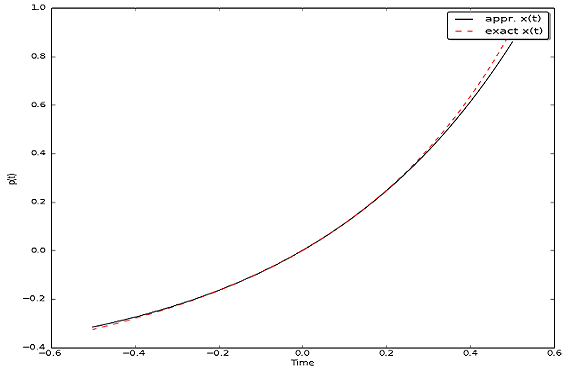
Figure 1. Plots of exact and approximate solutions.

Consider again the system of Example 3. Assume we are interested in the behaviours described by $S=\{x,y,z,w\}$. The following reduced linear system in the variables $\mathrm{\mathbf{y}}=(y_{1},y_{2},y_{3})^{T}$, which guarantees an approximation of order $m=3$ for those behaviours, can be obtained by applying the method.

$$\left\{\begin{array}[]{rclclcl}\dot{y}_{1}&=&3y_{1}/2&+&\sqrt{5}y_{2}/10&+&\sqrt{30}y_{3}/30\\ \dot{y}_{2}&=&\sqrt{5}y_{1}/2&+&11y_{2}/10&+&\sqrt{6}y_{3}11/30\\ \dot{y}_{3}&=&&&\sqrt{6}y_{2}/5&+&4y_{3}/10\\ \mathrm{\mathbf{y}}(0)&=&\lx@intercol(2,0,0)^{T}\,.\hfil\lx@intercol\end{array}\right.$$ (32)

We do not report the full $4\times 3$ matrix $B$ here, but only mention that, following Theorem 17, the approximated version of $x(t)$ can be obtained from $\mathrm{\mathbf{y}}(t)$ as: $\hat{x}(t)=(1,0,0,0)\cdot B\mathrm{\mathbf{y}}(t)=\sqrt{5}y_{2}(t)/5-\sqrt{30}y_{3}(t)/10$. The plots in Figure 1 show that the approximation is quite good around $t=0$.

We finally give a sufficient condition for exactness. This condition applies, for example, to linear systems, that is when the drifts $f_{i}$ in $F$ are linear functions. Consider the sequence of Krylov spaces $K_{1},K_{2},...$ that can be built according to equation (26). A Krylov space $K_{m}$ is said to be invariant if $K_{m+1}\subseteq K_{m}$. Of course there always exists $m\leq M$ such that $K_{m}$ is invariant; moreover the condition of invariance for $K_{m}$ can be efficiently detected (see [35]).

Corollary 18.

Assume $\mathcal{M}$ includes all monomials in $\cup_{j\geq 0}\mathcal{L}^{(j)}(S)$. Choose $m$ such that $K_{m}$ is invariant. Then, with the notation introduced above, $p(\mathrm{\mathbf{x}}(t))=p^{T}B\mathrm{\mathbf{y}}(t)$.

Proof 7.3.

Under the given condition, $\mathcal{L}^{(j)}(p)=Lp$ for any $j\geq 0$ and $p\in S$. Moreover, since $K_{m}=K_{m+1}=\cdots$, the statement in Lemma 16 also holds for any $j\geq m$, hence for any $j$. This allows one to extend the proof given in 17 to prove that the Taylor coefficients of $p(\mathrm{\mathbf{x}}(t))$ and $(p^{T}B)\mathrm{\mathbf{y}}(t)$ are all the same.

Remark 19 (on computing the matrices $A$ and $B$).

There exist relatively efficient and numerically stable methods to build the pair of matrices $A$ and $B$ needed in the construction of the reduced system. One of these methods is the Arnoldi algorithm [3, 35], which takes $O(Nz\cdot m)$ floating-point operations, and as much memory if a sparse storage scheme is adopted. Here $Nz$ denotes the number of nonzero elements in the matrix $L$: this is $O(M^{2})$ in the worst case, but it will be typically much smaller, as polynomials arising in applications tend to be sparse. Moreover, the method need not a fully stored matrix $L$, but only a handle to the matrix-vector multiplication function $u\mapsto L^{T}u$. Using appropriate data structures, this method can be implemented according to an ‘on-the-fly’ strategy, where the terms are unfolded as needed.

8. Examples

Although the focus of the present paper is mostly on theory, it is instructive to put a proof-of-concept implementation of our algorithms at work on a few simple examples taken from the literature. We illustrate below two cases, a linear and a nonlinear system.

8.1. Example 1: linearity and weighted automata

The purpose of this example is to argue that, when the transition structure induced by the Lie-derivatives is considered, $\mathcal{L}$-bisimilarity is fundamentally a linear-time semantics. We first introduce weighted automata, a more compact way of representing the transition structure of the coalgebra $C_{\mathbf{\Phi}}$.

A (finite- or infinite-state) weighted automaton is like an ordinary automaton, save that both states and transitions are equipped with weights from $\mathbb{R}$. Given $F$ and $v_{0}$, we can build a weighted automaton with monomials as states, weighted transitions given by the rule $\alpha\xrightarrow{\;\lambda\;}\beta$ iff $\mathcal{L}_{F}(\alpha)=\lambda\beta+q$ for some polynomial $q$ not comprising $\beta$ as a monomial, and real $\lambda\neq 0$, and where each state $\alpha$ is assigned weight $\alpha(v_{0})$. As an example, consider the weighted automaton in Figure 2, where the state weights (not displayed) are 1 for $x_{10}$, and 0 for any other state.

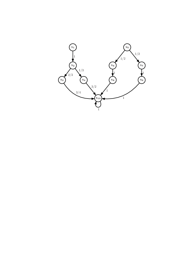
Figure 2. A weighted automaton.

This automaton is generated – and in fact codes up – a system of ode’s with ten variables, where $\dot{x}_{1}=x_{2}$, $\dot{x}_{2}=(2/3)x_{3}+(1/3)x_{4}$ etc., with the initial condition as specified by the state weights ($x_{1}(0)=0$ etc.).

A run in a weighted automaton is a path in the graph from a state to a state. The run’s weight is the product of all involved transition weights and the last state’s weight. In the standard linear-time semantics of weighted automata, each state $\alpha$ is assigned a function $\sigma_{\alpha}:\mathbb{N}\rightarrow\mathbb{R}$ (a stream, in the terminology of Rutten [34]) such that $\sigma_{\alpha}(i)$ is obtained by summing up all the weights of the runs involving $i$ transitions starting from $s$; e.g. $\sigma_{x_{1}}(3)=1\times\frac{2}{3}\times\frac{3}{4}+1\times\frac{1}{3}\times\frac{3}{2}=1$. Standard results in coalgebra (or a simple direct proof) ensure that this semantics is in agreement with bisimulation, in the sense that for any pair of states (in our case, monomials) $\alpha$ and $\beta$, $\alpha\sim_{\mathbf{\Phi}}\beta$ if and only $\sigma_{\alpha}=\sigma_{\beta}$; we refer the interested reader to [34, 6] for details on this construction and result.

When applied to our example, these results imply for instance that $x_{1}(t)=x_{5}(t)$. In fact, when invoked with this system and $\pi=\sum_{i=1}^{10}a_{i}x_{i}$ as inputs, the double chain algorithm terminates at $m=2$ (in about 0.3 s; this being a linear system, Gröbner bases are never actually needed), returning $\pi[V_{2}]=a_{1}(x_{6}-x_{7})+a_{2}(x_{8}-x_{9})+a_{3}(x_{6}-x_{2})+a_{4}(x_{5}-x_{1})+a_{5}(\frac{3}{2}x_{8}-x_{4})+a_{6}(\frac{3}{4}x_{8}-x_{3})$. This implies the expected equality $x_{1}=x_{5}$ (let $a_{4}=1$ and $a_{i}=0$ for $i\neq 4$ in the returned template), as well as other equalities, such as $x_{2}=x_{6}=x_{7}$ and $x_{8}=x_{9}$. All in all, $V_{2}$ being a 6-dimensional space, we will have a 4-dimensional $W=V_{2}^{\bot}$, that is a minimal system with 4 equations, a 60% reduction.

8.2. Example 2: nonlinear conservation laws

The law of the simple pendulum is $\frac{d^{2}}{dt^{2}}\theta=\frac{g}{\ell}\cos\theta$, where $\theta$ is the angle from the roof to the rod measured clockwise, $\ell$ is the length of the rod and $g$ is gravity acceleration (see picture on the right). If we assume the initial condition $\theta(0)=0$, this can be translated into the polynomial initial value problem below, where $\mathrm{\mathbf{x}}=(\theta,\omega,x,y)^{T}$. The meaning of the variables is $\omega=\dot{\theta}$, $x=\cos\theta$ and $y=\sin\theta$. We assume for simplicity $\ell=1$ and $g=9$.

$$\left\{\begin{array}[]{rcl}\dot{\theta}&=&\omega\\ \dot{\omega}&=&\frac{g}{\ell}x\\ \dot{x}&=&-y\omega\\ \dot{y}&=&x\omega\\ \mathrm{\mathbf{x}}(0)&=&(0,0,\ell,0)^{T}\,.\end{array}\right.$$

For this system, the double chain algorithm reports that there is no nontrivial linear conservation law (after $m=6$ iterations and about 0.3 s). We then ask the algorithm to find all the conservation laws of order two, that is we use the template ($\alpha$ ranges over monomials) $\pi=\sum_{\alpha_{i}\,:\,\deg(\alpha_{i})\leq 2}a_{i}\alpha_{i}$ as input. The algorithm terminates after $m=16$ iterations (in about 7 s). The invariant $J_{16}$ contains all the wanted conservation laws. The returned Gröbner basis for it is $G=\{x^{2}+y^{2}-1,\omega^{2}-18y\}$. The first term here just expresses the trigonometric identity $(\cos\theta)^{2}+(\sin\theta)^{2}=1$. Recalling that the (tangential) speed of the bob is $v=\ell\dot{\theta}=\ell\omega$, and that its vertical distance from the roof is $h=\ell\sin\theta=\ell y$, we see that the second term, considering our numerical values for $\ell,g$, is equivalent to the equation $\frac{1}{2}v^{2}=gh$, which, when multiplied by the mass $m$ of the bob, yields the law of conservation of energy $\frac{1}{2}mv^{2}=mgh$ (acquired kinetic energy = lost potential energy).

9. Conclusion, further and related work

We have presented a framework for automatic reasoning and reduction in systems of polynomial ode’s. In particular, we offer algorithms to: (1) compute the most general set of identities valid in the system that fit a user-specified template; and, (2) build a minimal system equivalent to the original one. These algorithms are based on a mix of simple algebraic and coalgebraic techniques.

9.1. Directions for further work

Scalability of our approach is an issue, as, already for simple systems, the Gröbner basis construction involved in the double chain algorithm can be computationally quite demanding. Further experimentation, relying on a well-engineered implementation of the method, and considering sizeable case studies, is called for in order to assess this aspect. One would also like to extend the present approach so as to deal with regions of possible initial values, rather than fixing one such value. This is important, e.g., in the treatment of hybrid systems (see below). After the short version of the present paper [9] appeared, some preliminary progress towards this goal has been made, see [10]. Concerning minimization, we note that the reduced system may not preserve the structure of the original one, e.g. as to the meaning of variables: this may be problematic in certain application domains, such as system biology. In the future, we intend to investigate this issue. Approximate reductions in the sense of System Theory [1] are also worth investigating. One problem of the approach described in Section 7 is that the reduced system depends on a fixed initial condition $v_{0}$. Obtaining bounds on the approximation error is another aspect that deserves further investigation. Some preliminary progress on these issues is reported in [11].

9.2. Related work

Bisimulations for weighted automata are related to our approach, because, as argued in subsection 8.1, Lie-derivation can be naturally represented by such an automaton. Algorithms for computing largest bisimulations on finite weighted automata have been studied by Boreale et al. [7, 6]. A crucial ingredient in these algorithms is the representation of bisimulations as finite-dimensional vector spaces. Approximate versions of this technique have also been recently considered in relation to Markov chains [8]. As discussed in Remark 10, in the case of linear systems, the algorithm in the present paper reduces to that of [7, 6]. Algebraically, moving from linear to polynomial systems corresponds to moving from vector spaces to ideals, hence from linear bases to Gröbner bases. From the point of view automata, this step leads to considering infinite weighted automata. In this respect, the present work may be also be related to the automata-theoretic treatment of linear ode’s by Fliess and Reutenauer [21].

Although there exists a rich literature dealing with linear aggregation of systems of ode’s (e.g. [1, 25, 40, 27]), we are not aware of fully automated approaches to minimization (Theorem 14), with the notable exception of a series of recent works by Cardelli and collaborators [14, 15, 16]. Mostly related to ours is [14]. There, for an extension of the polynomial ode  format called IDOL, the authors introduce two flavours of differential equivalence, called Forward (fde) and Backward (bde). They provide a symbolic, SMT-based partition refining algorithms to compute the largest equivalence of each type. fde groups variables in such a way that the corresponding quotient system recovers the sum of the original solutions in each class, whatever the initial condition. However, precise information on the individual original solutions cannot in general be recovered from the reduced system. In bde, variables grouped together are guaranteed to have the same solution. Therefore the quotient system permits in this case to fully recover the original solutions. As such, bde can be compared directly to our $\mathcal{L}$-bisimulation.

An important difference is that bde  may tell apart variables that have the same solution. As already seen, this is not the case with $\mathcal{L}$-bisimilarity, which is correct and complete. An important consequence of this difference is that the quotient system produced by bde is not minimal, whereas that produced by $\mathcal{L}$-bisimulation is, in a precise sense. In concrete cases, this may imply a significant size difference. For example, in the linear system of Subsection 8.1, bde finds only two equalities, leading to a quotient system of eight states; on the other hand, the minimal system produced by $\mathcal{L}$-bisimulation has four states. For what concerns reasoning, we note that, being based on partitions of variables, bde cannot express relations involving polynomial, or even linear, combinations of variables. Finally, the approach of [14] and ours rely on two quite different algorithmic decision techniques, SMT and Gröbner bases, both of which have exponential worst-case complexity. As shown by the experiments reported in [14], in practice bde and fde have proven quite effective at system reduction. At the moment, we lack similar experimental evidence for $\mathcal{L}$-bisimilarity. We also note that, limited to the case of polynomials of degree two, a polynomial algorithm for bde exists [15].

Linear aggregation and lumping of (polynomial) systems of ode’s are well known in the literature, se e.g. [1, 27, 25, 40] and references therein. However, as pointed out by Cardelli et al. [14], no general algorithms for computing the largest equivalence, hence the minimal exact reduction (in the sense of our Theorem 14) was known.

The seminal paper of Sankaranarayanan, Sipma and Manna [37] introduced polynomial ideals to find invariants of hybrid systems. Indeed, the study of the safety of hybrid systems can be shown to reduce constructively to the problem of generating invariants for their differential equations [30]. The results in [37] have been subsequently refined and simplified by Sankaranarayanan using pseudoideals [38], which enable the discovery of polynomial invariants of a special form. Other authors have adapted this approach to the case of imperative programs, see e.g. [12, 26, 32] and references therein. Reduction and minimization seem to be not a concern in this field.

Platzer has introduced differential dynamic logic to reason on hybrid systems [29]. The rules of this logic implement a fundamentally inductive, rather than coinductive, proof method. Mostly related to ours is Ghorbal and Platzer’s recent work on polynomial invariants [23]. One one hand, they characterize algebraically invariant regions of vector fields – as opposed to initial value problems, as we do. On the other hand, they offer sufficient conditions under which the trajectories induced by specific initial values satisfy all instances of a polynomial template (cf. [23, Prop.3]). The latter result compares with ours, but the resulting method appears to be not (relatively) complete in the sense of our double chain algorithm. Moreover, the computational prerequisites of [23] (symbolic linear programming, exponential size matrices, symbolic root extraction) are very different from ours, and much more demanding. Again, minimization is not addressed.

Ideas from Algebraic Geometry have been fruitfully applied also in Program Analysis. Relevant to our work is Müller-Olm and Seidl’s [26], where an algorithm to compute all polynomial invariants up to a given degree of an imperative program is provided. Similarly to what we do, they reduce the core problem to a linear algebraic one. However, being the setting in [26] discrete rather than continuous, the techniques employed there are otherwise quite different, mainly because: (a) the construction of the ideal chain is driven by the program’s operational semantics, rather than by Lie derivatives; (b) the found polynomial invariants must be valid under all initial program states, not just under the user specified one. If transferred to a continuous setting, condition (b) would lead in most cases to trivial invariants.

In nonlinear Control Theory, there is a huge amount of literature on Model Order Reduction (mor), that aims at reducing the size of a given system, while preserving some properties of interest, such as stability and passivity. A well established approach relies on building truncated Taylor expansions of the given sysytems [24, 28], repeated at various points along a trajectory of interest, to keep the approximation error globally small: a technique known as trajectory piece-wise linear (tpwl) mor, see e.g. [31]. One wonders whether our approximate linearization technique of Section 7 might conveniently serve as a building block of this strategy.

The present paper is the extended and revised version of [9]. W.r.t. [9], here we include complete proofs, the discussion of up-to techniques in Section 3, the approximate linearization technique of Section 7 and an extended and updated discussion of further and related work in the present section.

Appendix A Proofs and additional technical material

A.1. Proofs

Proof A.1 (Proof of Theorem 5.).

We check each of the equivalences (9–12) in turn.

• If $p\sim_{\mathbf{\Phi}}q$ then $p-q\in\ker(\sim_{\mathbf{\Phi}})$ by definition of $\ker$. Conversely, assume $p-q\in{\ker(\sim_{\mathbf{\Phi}})}$ $\subseteq$ $\big{\langle}\,\,\ker(\sim_{\mathbf{\Phi}})\,\,\big{\rangle}$. Since, by first part of Lemma 4 with $R=\sim_{\mathbf{\Phi}}$, the last set is an invariant, by the second part of the same lemma we obtain the wanted $p\sim_{\mathbf{\Phi}}q$, hence (9).

• Since $p\sim_{\mathbf{\Phi}}q$ implies $(p-q)(t)=0$, and $r(t)=0$ implies $r\sim_{\mathbf{\Phi}}0$ (in both cases by Theorem 1), from the definition of $\ker(\sim_{\mathbf{\Phi}})$ the second equality (10) immediately follows.

• A polynomial behaviour $p(\mathrm{\mathbf{x}}(t))$ is identically 0 in $\mathcal{A}$ if and only if all its derivatives $\frac{d}{dt^{j}}p(\mathrm{\mathbf{x}}(t))$, $j\geq 0$, vanish at 0, and this, via (7) and (5), yields (11).

• Note that if $p\in I$, with $I$ an invariant, then $p^{(j)}(v_{0})=0$ for each $j\geq 0$ (easily shown by induction on $j$). Conversely, if $p^{(j)}(v_{0})=0$ for each $j$, then $J=\big{\langle}\,\,\{p,p^{(1)},p^{(2)},...\}\,\,\big{\rangle}$ is an invariant and contains $p$. To check invariance of $J$, consider a generic $q\in J$, $q=\sum_{i}h_{i}p^{(j_{i})}$: it is immediate that $q(v_{0})=0$ and that $\mathcal{L}(q)=\sum_{i}\mathcal{L}(h_{i})p^{(j_{i})}+\sum_{i}h_{i}p^{(j_{i}+1)}\in J$. This way we have also proven the last equation (12).

Proof A.2 (Proof of Lemma 6.).

We proceed by induction on $j$. The base case $j=1$ follows from the definition of $m$. Assuming by induction hypothesis that $V_{m}=\cdots=V_{m+j}$ and that $J_{m}=\cdots=J_{m+j}$, we prove now that $V_{m}=V_{m+j+1}$ and that $J_{m}=J_{m+1+1}$. The key to the proof is the following fact

$$\pi^{(m+j+1)}[v] \in J_{m}\;\;\text{ for each }v\in V_{m}\,.$$ (33)

From this fact the thesis will follow, indeed:

1. $V_{m}=V_{m+j+1}$. To see this, observe that for each $v\in V_{m+j}=V_{m}$ (the equality here follows from the induction hypothesis), it follows from (33) that $\pi^{(m+j+1)}[v]$ can be written as a finite sum of the form $\sum_{l}h_{l}\cdot\pi^{(j_{l})}[u_{l}]$, with $0\leq j_{l}\leq m$ and $u_{l}\in V_{m}$. As a consequence, $\pi^{(m+j+1)}[v](v_{0})=0$, which shows that $v\in V_{m+j+1}$. This proves that $V_{m+j+1}\supseteq V_{m+j}=V_{m}$; the reverse inclusion is obvious;

2. $J_{m}=J_{m+j+1}$. As a consequence of $V_{m+j+1}=V_{m+j}(=V_{m})$ (the previous point), we can write

   $$J_{m+j+1} = \big{\langle}\,\,\cup_{i=0}^{m+j}\pi^{(i)}[V_{m+j}]\cup\pi^{(m+j+1)}[V_{m+j}]\,\,\big{\rangle}$$

   $$= \big{\langle}\,\,J_{m+j}\cup\pi^{(m+j+1)}[V_{m+j}]\,\,\big{\rangle}$$

   $$= \big{\langle}\,\,J_{m}\cup\pi^{(m+j+1)}[V_{m}]\,\,\big{\rangle}$$

   where the last step follows by induction hypothesis. From (33), we have that $\pi^{(m+j+1)}[V_{m}]\subseteq J_{m}$, which implies the thesis for this case, as $\big{\langle}\,\,J_{m}\,\,\big{\rangle}=J_{m}$.

We prove now (33). Fix any $v\in V_{m}$. First, note that $\pi^{(m+j+1)}[v]=\mathcal{L}(\pi^{(m+j)}[v])$ (here we are using (13)). As by induction hypothesis $\pi^{(m+j)}[V_{m}]=\pi^{(m+j)}[V_{m+j}]\subseteq J_{m+j}=J_{m}$, we have that $\pi^{(m+j)}[v]$ can be written as a finite sum $\sum_{l}h_{l}\cdot\pi^{(j_{l})}[u_{l}]$, with $0\leq j_{l}\leq m$ and $u_{l}\in V_{m}$. Applying the rules of Lie derivatives (2), (3), we find that $\pi^{(m+j+1)}[v]=\mathcal{L}(\pi^{(m+j)}[v])$ equals

$$\sum_{l}\left(h_{l}\cdot\pi^{(j_{l}+1)}[u_{l}]+\mathcal{L}(h_{l})\cdot\pi^{(j_{l})}[u_{l}]\right)\,.$$

Now, for each $u_{l}$, $u_{l}\in V_{m}=V_{m+1}$, each term $\pi^{(j_{l}+1)}[u_{l}]$, with $0\leq j_{l}+1\leq m+1$, is by definition in $J_{m+1}=J_{m}$. This shows that $\pi^{(m+j+1)}[v]\in J_{m}$, as required.

Proof A.3 (Proof of Corollary 15.).

Concerning the first part, let us denote by $\mathcal{Z}_{\mathbf{\Psi}}$ the largest invariant induced by $\mathbf{\Psi}$ in the polynomial ring $\mathbb{R}[\mathrm{\mathbf{y}}]$, according to Theorem 5. We have: $p\sim_{\mathbf{\Phi}}q$ in $\mathbb{R}[\mathrm{\mathbf{x}}]$ if and only if $(p-q)\in\mathcal{Z}_{\mathbf{\Phi}}$ (Theorem 5(10)) if and only if $(p-q)\circ\mathrm{\mathbf{x}}(t)=0$ (Theorem 5(9)) if and only if $(p-q)\circ B\mathrm{\mathbf{y}}(t)=0$ (Theorem 13) if and only if $(p(B\mathrm{\mathbf{y}})-q(B\mathrm{\mathbf{y}}))\left(t\right)=0$ if and only if $(p(B\mathrm{\mathbf{y}})-q(B\mathrm{\mathbf{y}}))\in\mathcal{Z}_{\mathbf{\Psi}}$ (Theorem 5(9)) if and only if $p(B\mathrm{\mathbf{y}})\sim_{\mathbf{\Psi}}q(B\mathrm{\mathbf{y}})$ in $\mathbb{R}[\mathrm{\mathbf{y}}]$ (Theorem 5(10)).

Concerning the second part, denoting by $e_{i}$ the $i$-th canonical vector in $\mathbb{R}^{N}$, note that: $x_{i}\sim_{\mathbf{\Phi}}x_{j}$ if and only if $x_{i}-x_{j}\in\mathcal{Z}_{\mathbf{\Phi}}$ if and only if $e_{i}-e_{j}\in V_{m}$ if and only if $e_{i}-e_{j}\bot W$ if and only if $B^{T}(e_{i}-e_{j})=0$, from which the thesis follows for this case.

A.2. Pseudoideals

We briefly discuss a sufficient condition for establishing the condition (19), that is $J_{i+1}=J_{i}$, which does not involve Gröbner bases, but only linear algebraic computations, and can therefore lead to a gain in efficiency. We ill make use of a bit of new notation. For a set of polynomials $S$ and an integer $k\geq 0$, denote by $\big{\langle}\,\,S\,\,\big{\rangle}_{k}$ the subset of $\big{\langle}\,\,S\,\,\big{\rangle}$ generated from $S$ by only using multiplier polynomials $h_{j}$ of degree $\leq k$ (cf. equation (8)); this is a pseudo ideal of degree $k$, in the terminology of Colón [19]. We can choose $k\geq 0$ and replace (19) by the following stronger condition

$$\pi^{(i+1)}[B_{i}] \subseteq \big{\langle}\,\,\cup_{j=0}^{i}\pi^{(j)}[B_{i}]\,\,\big{\rangle}_{k}\,.$$ (34)

If (34) is true then of course also (19) is true, while the converse is not valid in general. Condition (34) can be checked by linear algebraic techniques, which do not involve Gröbner bases computations. Indeed, a pseudo ideal $\big{\langle}\,\,S\,\,\big{\rangle}_{k}$ has the structure of a vector space over $\mathbb{R}$ of dimension $|S|\cdot M$, where $M$ is the number of distinct monomials of degree $\leq k$. However, the resulting algorithm is not guaranteed to terminate.

A.3. Building an orthonormal basis of $V^{\bot}$

We use here to the terminology of Section 6. Let us first work out a convenient characterization of the space $W=V^{\bot}$. Consider the successive Lie derivatives of the vector $\mathrm{\mathbf{x}}=(x_{1},...,x_{N})^{T}$, taken componentwise, that is the vectors of polynomials $\mathrm{\mathbf{x}}^{(j)}=(x_{1}^{(j)},...,x_{N}^{(j)})^{T}$, for $j=0,1,..$. Once evaluated at $v_{0}$, these become vectors in $\mathbb{R}^{N}$. We claim that

$$W = \mathrm{span}\left\{\mathrm{\mathbf{x}}(v_{0}),\mathrm{\mathbf{x}}^{(1)}(v_{0}),...,\mathrm{\mathbf{x}}^{(m)}(v_{0})\right\}\,.$$ (35)

Indeed, we have, by definition of $V$ (here $v=(\lambda_{1},...,\lambda_{N})^{T}$ denotes a generic vector in $\mathbb{R}^{N}$)

$$V = V_{m}$$

$$= \left\{v\,:\,\sum_{i=1}^{N}\lambda_{i}x^{(j)}_{i}(v_{0})=0\text{ for }j=0,...,m\right\}$$

$$= \left\{v\,:\,\langle v,\mathrm{\mathbf{x}}^{(j)}(v_{0})\rangle=0\text{ for }j=0,...,m\right\}$$

$$= \left\{\mathrm{\mathbf{x}}(v_{0}),\mathrm{\mathbf{x}}^{(1)}(v_{0}),...,\mathrm{\mathbf{x}}^{(m)}(v_{0})\right\}^{\bot}$$

which is equivalent to (35). Note that $l=\dim(W)\leq m+1,N$ (and typically one will have $l\ll N$). Therefore, a way to build an orthonormal basis $B$ for $W$ is just to apply the Gram-Schmidt orthonormalization process to the set of vectors on the right-hand side of (35). This process can in fact carried out incrementally, as the vectors of Lie derivatives $\mathrm{\mathbf{x}}^{(j)}$ are computed.

References

- [1] A.C. Antoulas. Approximation of Large-scale Dynamical Systems. SIAM, 2005.
- [2] V.I. Arnold. Ordinary Differential Equations. The MIT Press, ISBN 0-262-51018-9, 1978.
- [3] W. E. Arnoldi. The principle of minimized iterations in the solution of the matrix eigenvalue problem. Quarterly of Applied Mathematics, vol. 9, pp. 17-29, 1951.
- [4] M. Bernardo. A survey of Markovian behavioral equivalences. In Formal Methods for Performance Evaluation, vol. 4486 of LNCS, pages 180-219. Springer, 2007.
- [5] M. L. Blinov, J. R. Faeder, B. Goldstein, and W. S. Hlavacek. BioNet-Gen: software for rule-based modeling of signal transduction based on the interactions of molecular domains. Bioinformatics, 20(17): 3289-3291, 2004.
- [6] F. Bonchi, M.M. Bonsangue, M. Boreale, J.J.M.M. Rutten, and A. Silva. A coalgebraic perspective on linear weighted automata. Inf. Comput. 211: 77-105, 2012.
- [7] M. Boreale. Weighted Bisimulation in Linear Algebraic Form. Proc. of CONCUR 2009, LNCS 5710, pp. 163-177, Springer, 2009.
- [8] M. Boreale. Analysis of Probabilistic Systems via Generating Functions and Padé Approximation. ICALP 2015 (2): 82-94, LNCS 9135, Springer, 2015. Extended version available as DiSIA working paper 2016/10, http://local.disia.unifi.it/wp_disia/2016/wp_disia_2016_10.pdf.
- [9] M. Boreale. Algebra, coalgebra, and minimization in polynomial differential equations. In Proc. of FoSSACS 2017:71–87, LNCS 10203, Springer, 2017. Conference version of the present paper.
- [10] M. Boreale. Complete algorithms for algebraic strongest postconditions and weakest preconditions in polynomial ode’s. In Proc. of SOFSEM’18, LNCS 10706: 442–455, Springer. Full version available as http://arxiv.org/abs/1708.05377, 2017.
- [11] M. Boreale. Algorithms for exact and approximate linear abstractions of polynomial continuous systems. HSCC 2018: 207–216, ACM, 2018.
- [12] D. Cachera, Th. Jensen, A. Jobi, and F. Kirchner. Inference of Polynomial Invariants for Imperative Programs: A Farewell to Gröbner Bases. SAS 2012, LNCS 7460: 58-74, Springer, 2012.
- [13] L. Cardelli. On process rate semantics. Theoretical Computer Science, 391(3):190-215, 2008.
- [14] L. Cardelli, M. Tribastone, M. Tschaikowski, and A. Vandin. Symbolic Computation of Differential Equivalences, POPL 2016, ACM, 2016.
- [15] L. Cardelli, M. Tribastone, M. Tschaikowski, and A. Vandin. Efficient Syntax-driven Lumping of Differential Equations, TACAS 2016:93-111, LNCS 9636, Springer, 2016.
- [16] L. Cardelli, M. Tribastone, M. Tschaikowski, and A. Vandin. Comparing Chemical Reaction Networks: A Categorical and Algorithmic Perspective, LICS 2016, IEEE, 2016.
- [17] L. Cardelli, M. Tribastone, M. Tschaikowski, and A. Vandin. ERODE: Evaluation and Reduction of Ordinary Differential Equations. Available from http://sysma.imtlucca.it/tools/erode/.
- [18] F. Ciocchetta and J. Hillston. Bio-PEPA:A framework for the modelling and analysis of biological systems. Theoretical Computer Science, 410 (33-34):3065-3084, 2009
- [19] M. Colón. Polynomial approximations of the relational semantics of imperative programs. Science of Computer Programming 64: 76-9, 2007.
- [20] D. Cox, J. Little, and D. O’Shea. Ideals, Varieties, and Algorithms An Introduction to Computational Algebraic Geometry and Commutative Algebra. Undergraduate Texts in Mathematics, Springer, 2007.
- [21] M. Fliess, and C. Reutenauer. Theorie de Picard-Vessiot des Systèmes Reguliers. Colloque Nat. CNRS-RCP567, Belle-ile sept. 1982, in Outils et Modèles Mathématiques pour l’Automatique l’Analyse des systèmes et le tratement du signal. CNRS, 1983.
- [22] H.P. Gumm, Tobias Schröder. Covarieties and complete covarieties. Theoretical Computer Science 260(1):71-86, Elsevier, 2001.
- [23] K. Ghorbal, A. Platzer. Characterizing Algebraic Invariants by Differential Radical Invariants. TACAS 2014: 279-294, 2014. Extended version available from http://reports-archive.adm.cs.cmu.edu/anon/2013/CMU-CS-13-129.pdf.
- [24] P. Li and L. Pileggi. Compact reduced-order modeling of weakly nonlinear analog and RF circuits. IEEE Trans. Comput.-Aided Des. Integr. Circuits Syst., vol. 24, no. 2, pp. 184-203, 2005.
- [25] G. Li, H. Rabitz, and J. Tóth. A general analysis of exact nonlinear lumping in chemical kinetics. Chemical Engineering Science 49 (3), 343-361, 1994.
- [26] M. Müller-Olm and H. Seidl. Computing polynomial program invariants. Information Processing Letters 91(5), 233-244, 2004.
- [27] M.S. Okino and M.L. Mavrovouniotis. Simplification of mathematical models of chemical reaction systems. Chemical Reviews, 2(98):391-408, 1998.
- [28] J.R. Phillips. Projection-based approaches for model reduction of weakly nonlinear time-varying systems. IEEE Trans. Comput.-Aided Des., vol. 22, no. 2, pp. 171-187, 2003.
- [29] A. Platzer. Differential dynamic logic for hybrid systems. J. Autom. Reasoning 41(2), 143-189, 2008.
- [30] A. Platzer. Logics of dynamical systems. In LICS 2012: 13-24, IEEE, 2012.
- [31] M. Rewienski and J. White. A trajectory piecewise-linear approach to model order reduction and fast simulation of nonlinear circuits and micromachined devices. IEEE Trans. Comput.-Aided Des., vol. 22, no. 2, pp. 155-170, 2003.
- [32] E. Rodríguez-Carbonell and D. Kapur. Generating all polynomial invariants in simple loops. Journal of Symbolic Computation 42(4), 443-476, 2007.
- [33] J. Roychowdhury. Reduced-order modelling of time-varying systems. IEEE Trans. Circuits Syst.-II: Analog Digital Signal Process., vol. 46, no. 10, pp. 1273-1288, 1999.
- [34] J.J.M.M. Rutten. Behavioural differential equations: a coinductive calculus of streams, automata, and power series. Theoretical Computer Science, 308(1–3): 1–53, 2003.
- [35] Y. Saad. Iterative methods for sparse linear systems. SIAM, 2003.
- [36] D. Sangiorgi. Beyond Bisimulation: The “up-to” Techniques. FMCO 2005: 161-171, 2005.
- [37] S. Sankaranarayanan, H. Sipma, and Z. Manna. Non-linear loop invariant generation using Gröbner bases. POPL 2004.
- [38] S. Sankaranarayanan. Automatic invariant generation for hybrid systems using ideal fixed points. HSCC 2010: 221-230, ACM, 2010.
- [39] A. Tiwari. Approximate reachability for linear systems. HSCC 2003: 514-525, ACM, 2003.
- [40] J. Tóth, G. Li, H. Rabitz, and A. S. Tomlin. The effect of lumping and expanding on kinetic differential equations. SIAM Journal on Applied Mathematics, 57(6):1531-1556, 1997.
- [41] M. Tribastone, S. Gilmore, and J. Hillston. Scalable differential analysis of process algebra models. IEEE Trans. Software Eng., 38(1):205-219, 2012.
- [42] E. O. Voit. Biochemical systems theory: A review. ISRN Biomathematics, 2013:53, 2013.