An efficient relativistic density-matrix renormalization group implementation in a matrix-product formulation

Abstract

We present an implementation of the relativistic quantum-chemical density matrix renormalization group (DMRG) approach based on a matrix-product formalism. Our approach allows us to optimize matrix product state (MPS) wave functions including a variational description of scalar-relativistic effects and spin–orbit coupling from which we can calculate, for example, first-order electric and magnetic properties in a relativistic framework. While complementing our pilot implementation (S. Knecht et al., J. Chem. Phys., 140, 041101 (2014)) this work exploits all features provided by its underlying non-relativistic DMRG implementation based on an matrix product state and operator formalism. We illustrate the capabilities of our relativistic DMRG approach by studying the ground-state magnetization as well as current density of a paramagnetic $f^{9}$ dysprosium complex as a function of the active orbital space employed in the MPS wave function optimization.

I Introduction

With the advent of the density-matrix renormalization group (DMRG) approach White (1992, 1993); Schollwöck (2005, 2011) in (non-relativistic) quantum chemistry Legeza et al. (2008); Chan et al. (2008); Chan and Zgid (2009); Marti and Reiher (2010, 2011); Chan and Sharma (2011); Wouters and van Neck (2014); Kurashige (2014); Yanai et al. (2015); Olivares-Amaya et al. (2015); Szalay et al. (2015); Knecht et al. (2016a); Chan et al. (2016), approximate solutions for a complete-active-space (CAS)-type problem within chemical accuracy became computationally feasible on a routine basis albeit the fact that variational optimization merely involves a polynomial number of parameters. The combination with a self-consistent-field orbital optimization ansatz (DMRG-SCF) Zgid and Nooijen (2008a); Ghosh et al. (2008); Zgid and Nooijen (2008b); Sun, Yang, and Chan (2017); Ma et al. (2017) makes active orbital spaces accessible that surpass the CASSCF limit by about five to six times. Yet, the construction of a (chemically) meaningful active orbital space poses a fundamental challenge that calls for automation Stein and Reiher (2016); Stein, von Burg, and Reiher (2016); Stein and Reiher (2017); Sayfutyarova et al. (2017). In contrast to early work on ab initio DMRG Schollwöck (2005), recent efforts on the quantum-chemical DMRG algorithm Schollwöck (2011) focused on a variational optimization of a special class of ansatz states called matrix product states (MPSs) Östlund and Rommer (1995); Verstraete, Porras, and Cirac (2004) in connection with a matrix-product operator (MPO) representation of the quantum-chemical Hamiltonian Murg et al. (2010); Keller et al. (2015); Keller and Reiher (2016); Chan et al. (2016); Nakatani .

Combining the principles of quantum mechanics Dirac (1948) and special relativity Einstein (1905) into relativistic quantum mechanics, Dirac Dirac (1928) put forward a (one-electron) theory which constitutes the central element of relativistic quantum chemistry Dyall and Fægri (2007); Reiher and Wolf (2009). In this framework, deviations in the description of the electron dynamics increase compared to (nonrelativistic) Schrödinger quantum mechanics as one considers electrons moving (in the vicinity of a heavy nucleus) at velocities close to the speed of light. Consequently, the differences between results of relativistic quantum calculations employing a finite and an infinite speed of light, respectively — which are for the latter case equivalent to results from conventional nonrelativistic calculations based on the Schrödinger equation — can serve as a definition for the chemical concept of “relativistic effects”.

The latter are commonly split into kinematic relativistic effects (sometimes also referred to as scalar-relativistic effects) and magnetic effects both of which grow approximately quadratic with the atomic number $Z$ Pyykkö (1988). A scalar-relativistic theory therefore considers only kinematic relativistic effects whereas a fully relativistic theory includes both kinematic relativistic and magnetic effects. Kinematic relativistic effects reflect changes of the non-relativistic kinetic energy operator while spin-orbit (SO) interaction, which is the dominant magnetic effect (for heavy elements), originates from a coupling of the electron spin to the induced magnetic field resulting from its orbital motion in the field created by the other charged particles, namely the nuclei and remaining electrons Saue (2011). Encounters of relativistic effects are ubiquitous in the chemistry and physics of heavy elements compounds, see for example Refs. 36, 37 and 40 and references therein. Besides kinematic relativistic effects, SO interactions are also expected to strongly influence the chemical bonding and reactivity in heavy-element containing molecular systems Cotton (2006); Schwerdtfeger (2014). For example, Ruud and co-workers Demissie et al. (2016) as well as Gaggioli et al. Gaggioli et al. (2016) recently highlighted distinguished cases of mercury- and gold-catalyzed reactions where SO coupling effects are driving the main reaction mechanisms by paving the way for catalytic pathways that would otherwise not even have been accessible.

Considering a prototypical molecular, open-shell lanthanide complex, we aim in this work at the calculation of (static) magnetic properties which either require SO-coupled wave functions such as molecular g-factors and electron-nucleus hyperfine coupling, which are central parameters in electron paramagnetic resonance (EPR) spectroscopy Harriman (1978); Kaupp, Bühl, and Malkin (2004), or assume a particular simple form in a relativistic framework, including, for example, the magnetization and current density Reiher and Wolf (2009). We will pay particular attention to the latter two properties since they play a particular role for the eligibility of open-shell lanthanide tags in spin-labeling of protein complexes Jeschke and Polyhach (2007); Clore and Iwahara (2009); Jeschke (2012); Goldfarb (2014); Bertini et al. (2017).

As open-shell electronic structures are often governed by strong electron correlation effects, their computational description calls for a multiconfigurational ansatz Szalay et al. (2012); Roca-Sanjuan, Aquilante, and Lindh (2012) which usually set out from a spin-free (non-relativistic or scalar-relativistic) formulation. Here, electron correlation is commonly split into a static contribution and a dynamic contribution with the latter often being treated in a subsequent step by (internally-contracted) multi-reference perturbation or configuration interaction theories Szalay et al. (2012); Roca-Sanjuan, Aquilante, and Lindh (2012). Their zeroth-order wave function is typically of CAS-type such as CASSCF or DMRG(-SCF) which are assumed to be able to adequately grasp static electron correlation effects. In this context, additional challenges may be encountered in particular for heavy-element complexes which arise from the large number of (unpaired) valence electrons to be correlated, i.e., the $(n-2)f\ (n-1)d\ ns\ np$ manifold of $f$-elements, as well as the occurrence of near-degeneracies of electronic states. To arrive at SO-coupled eigenstates in such a spin-free setting, requires then to invoke a so-called two-step SO procedure (see for example Refs. 54; 55; 56; 57; 58 for recent developments based on CAS- and DMRG-like formulations). Notably, this procedure relies on an additivity of electron correlation and SO effects or a weak polarization of orbitals due to SO interaction, or both. Moreover, it entails the need to take into account a priori a sufficiently large number of spin-free electronic states for the evaluation of the spin-orbit Hamiltonian matrix elements in order to ensure convergence of the SO-coupled eigenstates. Hence, the predictive potential of such two-step approaches is inevitably limited for a finite set of spin-free states. By contrast, a genuine relativistic DMRG model, initially proposed for a “traditional” (i.e. non-MPO based formulation) DMRG model in Ref. 59 and proposed in this work within an efficient MPS/MPO framework of the DMRG algorithm, addresses simultaneously all of the above issues by providing access to large active orbital spaces combined with a variational description of relativistic effects in the orbital basis.

The paper is organized as follows: We first briefly review the concept of representing a wave function and an operator in a matrix-product ansatz, respectively, including a short summary of the variational optimization of an MPS wave function in such a model. In Section III, a relativistic Hamiltonian framework suitable for a variational description of SO coupling is introduced and a detailed account of its implementation in an MPS/MPO setting of the DMRG ansatz is given. In addition, we illustrate the calculation of first-order molecular properties within our relativistic DMRG model. Subsequently, after providing computational details in Section IV.1, we assess in Section IV.2 the numerical performance of our present implementation with respect to the calculation of absolute energies for the sample molecule thallium hydride. In Section IV.3, we demonstrate the applicability of our relativistic MPS/MPO-based DMRG model for the calculation of magnetic properties in a real-space approach at the example of a large Dy(III)-containing molecular complex. Conclusions and an outlook concerning future work based on the presented relativistic DMRG model are summarized in Section V.

II Matrix product states and matrix product operators

We briefly introduce in this section the concepts of expressing a quantum state as an MPS and a (Hermitian) operator as an MPO in a non- or scalar-relativistic framework which will constitute the basis for our genuine relativistic DMRG model — including a variational account of SO coupling — discussed in Section III. Our notation closely follows the presentations of Refs. 30 and 60. A comprehensive review of the DMRG approach in an MPS/MPO formulation can be found in Ref. 4.

II.1 MPS

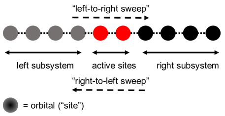
Figure 1: Alignment of orbitals (“sites”) of a given active orbital space on a fictitious (as indicated by the connecting $\cdots$) one-dimensional lattice. The latter is partitioned into a left and right subsystem as well as active sites on which DMRG many-electron basis states are constructed and successively optimized in a variational approach. While traversing (“sweeping”) through the lattice from left to right, the left subsystem is gradually enlarged by the left active site whereas the leftmost site on the right subsystem becomes active. Reaching the end of the lattice initiates a right-to-left sweep and the procedure is reversed.

Consider an arbitrary state $\left|\Psi\right>$ in a Hilbert space spanned by ($N$ electrons distributed in) $L$ spatial orbitals that are assumed to be ordered in a favorable fashion Keller and Reiher (2014) on a fictitious one-dimensional lattice. In a traditional (CI-like) ansatz, $\left|\Psi\right>$ is commonly expressed as a linear superposition of occupation number vectors (ONVs) $\left|\boldsymbol{k}\right>$ with the expansion coefficients $c_{k_{1}\ldots k_{L}}$

$$\left|\Psi\right>=\sum\limits_{{\boldsymbol{k}}}c_{\boldsymbol{k}}\left|\boldsymbol{k}\right>=\sum\limits_{k_{1},\ldots,k_{L}}c_{k_{1}\ldots k_{L}}\left|k_{1}\ldots k_{L}\right>\ .$$ (1)

Note that, in a non-relativistic formulation, each local space is of dimension four corresponding to the possible local basis states

$$k_{l}=\left\{\left|\uparrow\downarrow\right>,\left|\uparrow\right>,\left|\downarrow\right>,\left|0\right>\right\}\ ,$$ (2)

for the $l$-th spatial orbital. By contrast, in an MPS representation of $\left|\Psi\right>$, the CI coefficients $\{c_{k_{1}\ldots k_{L}}\}$ are written as a product of $m_{l-1}\times m_{l}$-dimensional matrices $M^{k_{l}}=\{M^{k_{l}}_{a_{l-1}a_{l}}\}$, i.e., four matrices corresponding to the local space dimension,

$$\left|\Psi\right> =\sum_{k_{1},\ldots,k_{L}}\sum_{a_{1},\ldots,a_{L-1}}M^{k_{1}}_{1a_{1}}M^{k_{2}}_{a_{1}a_{2}}\cdots M^{k_{L}}_{a_{L-1}1}\left|k_{1}\ldots k_{L}\right>=\sum_{\boldsymbol{k}}M^{k_{1}}M^{k_{2}}\cdots M^{k_{L}}\left|\boldsymbol{k}\right>\ .$$ (3)

Given the $\{c_{k_{1}\ldots k_{L}}\}$ being scalar coefficients, requires that the final contraction of the matrices $M^{k_{l}}$ must yield a scalar number. This further implies that the first and the last matrices in Eq. (3) are in practice $1\times m_{1}$-dimensional row and $m_{L-1}\times 1$-dimensional column vectors, respectively. The introduction of some maximum dimension $m$ for the matrices $M^{k_{l}}$, with $m$ commonly referred to as number of renormalized block states White (1993), constitutes the fundamental idea that facilitates to approximate a full CI-type wave function (cf. Eq. (1)) to chemical accuracy while merely requiring to optimize a polynomial number of parameters in an MPS wave function ansatz.

Moreover, the partitioning of the CI coefficients in products of the $M^{k_{l}}$ matrices given in Eq. (3) is not unique, i.e., $\left|\Psi\right>$ may be expressed (through successive applications of a singular value decomposition) in different ways such as in a left-canonical form Schollwöck (2011)

$$\left|\Psi\right>=\sum_{\boldsymbol{k}}A^{k_{1}}A^{k_{2}}\cdots A^{k_{L}}\left|\boldsymbol{k}\right>,$$ (4)

with

$$\sum_{k_{l}}A^{k_{l}\dagger}A^{k_{l}}=I\ ,$$ (5)

where $I$ is the unit matrix and the $A^{k_{l}}$ matrices are referred to as left-normalized MPS tensors. Similarly, the MPS can be written in right-canonical form Schollwöck (2011)

$$\left|\Psi\right>=\sum_{\boldsymbol{k}}B^{k_{1}}B^{k_{2}}\cdots B^{k_{L}}\left|\boldsymbol{k}\right>\ ,$$ (6)

where the $B^{k_{l}}$ matrices are right-normalized, satisfying the condition

$$\sum_{\sigma_{k}}B^{k_{l}}B^{k_{l}\dagger}=I\ .$$ (7)

The non-uniqueness, which allows us to express an MPS in different forms originates from the existence of a gauge degree of freedom Schollwöck (2011). Considering for a given MPS two adjacent sets of matrices $M^{k_{l}}$ and $M^{k_{l+1}}$ with matching bond dimensions $m$, it can be shown Schollwöck (2011) that the MPS is invariant with respect to a right (left) multiplication with matrix $X$ of dimension $m\times m$,

$$M^{k_{l}}\rightarrow M^{k_{l}}X\,\,\,\forall k_{l},\qquad\ M^{k_{l+1}}\rightarrow X^{-1}M^{k_{l+1}}\,\,\,\forall k_{l}\ ,$$ (8)

provided that $X$ is invertible and non-singular.

The gauge freedom may therefore be further exploited to express the MPS of Eq. (3) in mixed-canonical form at sites (orbitals) $\{l,l+1\}$ Schollwöck (2011)

$$\left|\Psi\right>=\sum_{\boldsymbol{k}}\sum_{a_{1},\cdots,a_{L-1}}A_{1a_{1}}^{k_{1}}\cdots A_{a_{l-2}a_{l-1}}^{k_{l-1}}M_{a_{l-1},a_{l+1}}^{k_{l}k_{l+1}}B_{a_{l+1}a_{l+2}}^{k_{l+2}}\cdots B_{a_{L-1}1}^{k_{L}}\left|\boldsymbol{k}\right>\ ,$$ (9)

where the MPS tensors $A^{k_{l-1}}=\{A^{k_{l-1}}_{a_{l-2}a_{l-1}}\}$ and $B^{k_{l-1}}=\{B^{k_{l+2}}_{a_{l+1}a_{l+2}}\}$ are left- and right-normalized, respectively, as shown in Eqs. (5) and (7) and $M_{a_{l-1},a_{l+1}}^{k_{l}k_{l+1}}$ is a two-site MPS tensor

$$M_{a_{l-1},a_{l+1}}^{k_{l}k_{l+1}}=\sum\limits_{a_{l}}M_{a_{l-1},a_{l}}^{k_{l}}M_{a_{l},a_{l+1}}^{k_{l+1}}\ .$$ (10)

The mixed-canonical form will be a central element of the two-site DMRG optimization algorithm outlined in Section II.3.

II.2 MPO

Exploiting the matrix-product formulation introduced in the previous section for operators, an $N$-electron operator $\widehat{W}$ can be expressed in MPO form as

$$\widehat{\mathcal{W}} = \sum_{k_{1},\ldots,k_{L}}\sum_{k_{1}^{\prime},\ldots,k_{L}^{\prime}}\sum_{b_{1},\ldots,b_{L-1}}W^{k_{1}k_{1}^{\prime}}_{1b_{1}}W^{k_{2}k_{2}^{\prime}}_{b_{1}b_{2}}\cdots W^{k_{L}k_{L}^{\prime}}_{b_{L-1}1}\left|k_{1}\ldots k_{L}\right>\left<k_{1}^{\prime}\ldots k_{L}^{\prime}\right|$$ (11)

$$\equiv \sum_{\boldsymbol{k}\boldsymbol{k^{\prime}}}w_{\boldsymbol{k}\boldsymbol{k^{\prime}}}\left|\boldsymbol{k}\right>\left<\boldsymbol{k^{\prime}}\right|\ ,$$

with the incoming and outgoing physical states $k_{l}$ and $k_{l}^{\prime}$ and the virtual indices $b_{l-1}$ and $b_{l}$. Rearranging the summations and changing the order of contraction in Eq. (11) leads to Keller et al. (2015); Keller and Reiher (2016)

$$\widehat{\mathcal{W}}=\sum\limits_{b_{1},\ldots,b_{L-1}}W^{1}_{1b_{1}}\cdots W^{l}_{b_{l-1}b_{l}}\cdots W^{L}_{b_{L-1}1}\ ,$$ (12)

where the entries of the $\left\{{W}^{l}_{b_{l-1}b_{l}}\right\}$ matrices comprise only local creation (annihilation) operators acting on the $l$-th orbital. For example, consider the operator $\tilde{a}_{\uparrow_{l}}^{\dagger}$ which can be written as a linear combination of the local basis states

$$\tilde{a}_{\uparrow_{l}}^{\dagger}=\left|\uparrow\downarrow\right>\left<\downarrow\right|+\left|\uparrow\right>\left<0\right|\ .$$ (13)

Hence, Eq. (13) implies that the matrix representation of $\tilde{a}_{\uparrow_{l}}^{\dagger}$ corresponds to a $(4\times 4)$-dimensional matrix with two non-zero entries equal to one. Likewise, similar considerations hold for the remaining local operators while the matrix representations of the corresponding local, relativistic operators of our relativistic DMRG model will be discussed in Section III.2.

For completeness, we conclude this section by considering the action of the local Hamiltonian $\hat{H}$ given in MPO form on an MPS state in mixed-canonical form (cf. Eq. (9)) at sites {$l,l+1$} which can be written as Schollwöck (2011)

$$\hat{H}\left|\Psi\right>=\sum_{b_{l-1},b_{l}}\sum_{a^{\prime}_{l-1},k^{\prime}_{l},a^{\prime}_{l}}L_{b_{l-1}}^{a_{l-1},a^{\prime}_{l-1}}W_{b_{l-1},b_{l+1}}^{k_{l}k_{l+1},k^{\prime}_{l}k^{\prime}_{l+1}}R_{b_{l+1}}^{a_{l+1},a^{\prime}_{l+1}}M_{a_{l-1},a_{l+1}}^{k^{\prime}_{l},k^{\prime}_{l+1}}|a_{l-1}\rangle_{A}|k_{l}\rangle|k_{l+1}\rangle|a_{l+1}\rangle_{B}\ ,$$ (14)

with the left and right basis states given by

$$|a_{l-1}\rangle_{A}=\sum_{k_{1},\cdots,k_{l-1}}\sum_{a_{1},\cdots,a_{l-1}}A_{1a_{1}}^{k_{1}}\cdots A_{a_{l-2}a_{l-1}}^{k_{l-1}}|k_{1},\cdots,k_{l-1}\rangle\ ,$$ (15)

and

$$|a_{l+1}\rangle_{B}=\sum_{k_{l+1},\cdots,k_{L}}\sum_{a_{l+1},\cdots,a_{L}}B_{a_{l+1}a_{l+2}}^{k_{l+2}}\cdots B_{a_{L-1}1}^{k_{L}}|k_{l+1},\cdots,k_{L}\rangle\ .$$ (16)

Here, we introduced the left and right boundaries as Schollwöck (2011); Keller et al. (2015)

$$L_{b_{l-1}}^{a_{l-1},a^{\prime}_{l-1}}=\sum_{\{a_{i},b_{i},a^{\prime}_{i};i<l-1\}}\left(\sum_{k_{1},k^{\prime}_{1}}A_{1,a_{1}}^{k_{1}\ast}W_{1,b_{1}}^{k_{1},k^{\prime}_{1}}A_{1,a^{\prime}_{1}}^{k^{\prime}_{1}}\right)\cdots\left(\sum_{k_{l-1},k^{\prime}_{l-1}}A_{a_{l-2},a_{l-1}}^{k_{l-1}\ast}W_{b_{l-2},b_{l-1}}^{k_{l-1},k^{\prime}_{l-1}}A_{a^{\prime}_{l-2},a^{\prime}_{l-1}}^{k^{\prime}_{l-1}}\right)\ ,$$ (17)

and

$$R_{b_{l+1}}^{a_{l+1},a^{\prime}_{l+1}} = \sum_{\{a_{i},b_{i},a^{\prime}_{i};i>l+1\}}\left(\sum_{k_{l+1},k^{\prime}_{l+1}}B_{a_{l+1},a_{l+2}}^{k_{l+2}\ast}W_{b_{l+1},b_{l+2}}^{k_{l+2},k^{\prime}_{l+2}}B_{a^{\prime}_{l+1},a^{\prime}_{l+2}}^{k^{\prime}_{l+2}}\right)\cdots$$ (18)

$$\times\left(\sum_{k_{L},k^{\prime}_{L}}B_{a_{L-1},a_{1}}^{k_{L}\ast}W_{b_{L-1},b_{1}}^{k_{L},k^{\prime}_{L}}B_{a^{\prime}_{L-1},a^{\prime}_{1}}^{k^{\prime}_{L}}\right)\ ,$$

as well as the two-site MPO tensor Schollwöck (2011); Keller et al. (2015)

$$W_{b_{l-1},b_{l+1}}^{k_{l}k_{l+1}k^{\prime}_{l}k^{\prime}_{l+1}}=\sum\limits_{b_{l}}W_{b_{l-1},b_{l}}^{k_{l}k^{\prime}_{l}}W_{b_{l},b_{l+1}}^{k_{l+1}k^{\prime}_{l+1}}\ .$$ (19)

II.3 Variational optimization of an MPS

In a variational optimization of $\left|\Psi\right>$ with the Hamiltonian $\hat{H}$ expressed in MPO form, the objective is to minimize the energy expectation value $\left<\Psi|\hat{H}|\Psi\right>$ with respect to the entries of the MPS tensors under the constraint that the wave function is normalized, i.e., $\left<\Psi|\Psi\right>=1$. To this end, a Lagrangian multiplier $\lambda$ is introduced to ensure normalization. The optimization of the MPS then corresponds to find the extremum of the Lagrangian Chan (2008)

$$\mathcal{L}=\left<\Psi\right|\hat{H}\left|\Psi\right>-\lambda\left<\Psi\right|\left.\Psi\right>.$$ (20)

The optimization parameters are the matrices $M^{k_{l}}$ of the MPS. To solve this highly non-linear optimization problem, the same idea as in the original (non-MPO) DMRG algorithm is adopted: iterating through the lattice and optimizing the entries $M_{a_{l-1,a_{l}}}^{k_{l}}$ of one matrix (single-site variant) or of the two-site MPS tensor $M_{a_{l-1},a_{l+1}}^{k_{l},k_{l+1}}$ (two-site variant) at a time, while keeping all the others fixed. This approach not only greatly simplifies the optimization problem to one of lower complexity but also ensures to find a better approximation to the true ground state in a variational sense.

In the following, we consider the two-site variant (corresponding to treating simultaneously two sites as “active” as indicated by a red color code in Figure 1). Taking the derivative with respect to the complex conjugate of $M_{a_{l-1},a_{l+1}}^{k_{l},k_{l+1}}$

$$\frac{\partial}{\partial M_{a_{l-1},a_{l+1}}^{k_{l},k_{l+1}\ast}}(\left<\Psi\right|\hat{H}\left|\Psi\right>-\lambda\left<\Psi\right|\left.\Psi\right>)=0\ ,$$ (21)

yields Schollwöck (2011)

$$\begin{split}\sum_{a^{\prime}_{l-1}a^{\prime}_{l},b_{l-1}b_{l+1}}\sum_{k^{\prime}_{l}k^{\prime}_{l+1}}L_{b_{l-1}}^{a_{l-1},a^{\prime}_{l-1}}W_{b_{l-1},b_{l+1}}^{k_{l}k_{l+1},k^{\prime}_{l}k^{\prime}_{l+1}}R_{b_{l+1}}^{a^{\prime}_{l+1},a_{l+1}}M_{a^{\prime}_{l-1},a^{\prime}_{l+1}}^{k^{\prime}_{l}k^{\prime}_{l+1}}=\lambda M_{a_{l-1},a_{l+1}}^{k_{l}k_{l+1}}\ ,\end{split}$$ (22)

where we assumed that the left and right boundaries (cf. Eqs. (17) and (18)) were calculated from left- and right-normalized MPS tensors, respectively.

The resulting Eq. (22) can be recast in a matrix eigenvalue equation Östlund and Rommer (1995); Schollwöck (2011)

$$\boldsymbol{\mathcal{{H}}}v-\lambda v=0\ ,$$ (23)

with the local Hamiltonian matrix $\boldsymbol{\mathcal{{H}}}$ at sites {$l,l+1$} after reshaping given by

$$H_{(k_{l,l+1}a_{l-1}a_{l+1}),(k^{\prime}_{l,l+1}a^{\prime}_{l-1}a^{\prime}_{l+1})}=\sum_{b_{l-1},b_{l+1}}L_{b_{l-1}}^{a_{l-1},a^{\prime}_{l-1}}W_{b_{l-1},b_{l+1}}^{k_{l}k_{l+1},k^{\prime}_{l}k^{\prime}_{l+1}}R_{b_{l+1}}^{a^{\prime}_{l+1},a_{l+1}}\ ,$$ (24)

and the vector $v$ collecting

$$v_{k_{l}k_{l+1}a_{l-1}a_{l+1}}=M_{a_{l-1},a_{l+1}}^{k_{l}k_{l+1}}\ .$$ (25)

Since we are often interested in only a few of the lowest eigenvalues $\lambda$, Eq. (23) is best solved by an iterative eigensolver such as the Jacobi-Davidson procedure. For example, having obtained the lowest eigenvalue $\lambda_{0}$ and the corresponding eigenvector $v^{0}_{k_{l}k_{l+1}a_{l-1}a_{l+1}}$, the latter can be reshaped back to $M_{a_{l-1},a_{l+1}}^{k_{l}k_{l+1}}$ which is then subject to a left- or right-normalization into $A^{k_{l}}_{a_{l-1}a_{l}}$ or $B^{k^{\prime}_{l+1}}_{a_{l}a_{l+1}}$ by a singular value decomposition (discarding the 3$m$ smallest singular values) in order to maintain the desired normalization structure and the dimensionality of the MPS tensors. Given the optimized MPS tensors for sites $l$ and $l+1$, the complete algorithm now sweeps sequentially forth and back from left-to-right and right-to-left through the lattice (cf. Figure 1) consisting of the $L$ spatial orbitals ordered in a suitable form. At each step the MPS tensors $\{M^{k_{l}}_{a_{l-1}a_{l}}\}$ are optimized until convergence is reached.

III Formulation of a relativistic DMRG model

III.1 Hamiltonian framework

In accordance with the pilot relativistic DMRG implementation presented in Ref. 59, our present formulation of a relativistic DMRG model in a matrix-product ansatz is based on the electronic, time-independent, external magnetic-field-free Dirac-Coulomb(-Breit) Hamiltonian (note that any two-component Hamiltonian is equally well applicable) which encompasses all important relativistic “corrections” Dyall and Fægri (2007); Reiher and Wolf (2009); Autschbach (2012) relevant for chemistry. Invoking the no-pair approximation, this operator can be written in second quantization as Jensen et al. (1996); Dyall and Fægri (2007),

$$\hat{H} = \sum_{pq}\left[h_{pq}{\hat{X}_{pq}^{+}}+\frac{1}{2}\left(h_{\bar{p}q}{\hat{X}_{\bar{p}q}^{+}}+h_{p\bar{q}}{\hat{X}_{p\bar{q}}^{+}}\right)\right]$$ (26)

$$+\frac{1}{2}\sum_{pqrs}\left[\left(pq|rs\right)\hat{x}^{++}_{pq,rs}+\left(\bar{p}q|rs\right)\hat{x}^{++}_{\bar{p}q,rs}+\left(p\bar{q}|rs\right)\hat{x}^{++}_{p\bar{q},rs}\right]$$

$$+\frac{1}{4}\sum_{pqrs}\left(\bar{p}q|r\bar{s}\right)\hat{x}^{++}_{\bar{p}q,r\bar{s}}$$

$$+\frac{1}{8}\sum_{pqrs}\left[\left(\bar{p}q|\bar{r}s\right)\hat{x}^{++}_{\bar{p}q,\bar{r}s}+\left(p\bar{q}|r\bar{s}\right)\hat{x}^{++}_{p\bar{q},r\bar{s}}\right]$$

$$-\frac{1}{2}\sum_{pqrs}\left[\left(p\boldsymbol{\alpha}q|r\boldsymbol{\alpha}s\right)\hat{x}^{--}_{pq,rs}+\left(\bar{p}\boldsymbol{\alpha}{q}|r\boldsymbol{\alpha}s\right)\hat{x}^{--}_{\bar{p}q,rs}+\left({p}\boldsymbol{\alpha}\bar{q}|r\boldsymbol{\alpha}s\right)\hat{x}^{--}_{p\bar{q},rs}\right]$$

$$-\frac{1}{4}\sum_{pqrs}\left(\bar{p}\boldsymbol{\alpha}q|r\boldsymbol{\alpha}\bar{s}\right)\hat{x}^{--}_{\bar{p}q,r\bar{s}}$$

$$-\frac{1}{8}\sum_{pqrs}\left[\left(\bar{p}\boldsymbol{\alpha}q|\bar{r}\boldsymbol{\alpha}s\right)\hat{x}^{--}_{\bar{p}q,\bar{r}s}+\left(p\boldsymbol{\alpha}\bar{q}|r\boldsymbol{\alpha}\bar{s}\right)\hat{x}^{--}_{p\bar{q},r\bar{s}}\right]\ ,$$

where the last three rows on the right-hand side of Eq. (26) comprise the two-electron terms originating from the Breit (Gaunt) interaction and the summation indices $p,q,r,s$ strictly refer to positive-energy spinors. Moreover, following earlier works Jensen et al. (1996); Thyssen, Fleig, and Jensen (2008); Kim and Lee (2013); Knecht, Legeza, and Reiher (2014); Bates and Shiozaki (2015), we assume in Eq. (26) a Kramers pair basis $\{\varphi_{l},\bar{\varphi}_{l}\}$ built from pairs of fermion spinor functions $\{\varphi_{l}\}$ and $\{\bar{\varphi}_{l}\}$, respectively. This implies that the summations in Eq. (26) run over Kramers pairs and not single spinors. According to Kramers theorem, which holds in the absence of an external magnetic field, states of a single fermion function $\{\varphi_{l}\}$ are (at least) doubly degenerate where each state is related to its energy-degenerate partner by time reversal Dyall and Fægri (2007); Reiher and Wolf (2009), i.e.,

$$\hat{\mathcal{K}}\varphi_{l}=\bar{\varphi}_{l}\ ,$$ (27)

where $\hat{\mathcal{K}}$ is the time-reversal operator. In addition, we employ in Eq. (26) Kramers single- ${\hat{X}}^{s}_{pq}$ (with $s=\pm$) and double replacement operators ${\hat{x}}^{s_{1},s_{2}}_{pq,rs}$ (with $s_{1},s_{2}=\pm$) Aucar, Jensen, and Oddershede (1995), respectively. They can be expressed in terms of creation and annihilation operators as Aucar, Jensen, and Oddershede (1995); Jensen et al. (1996); Fleig, Olsen, and Marian (2001); Dyall and Fægri (2007)

$${\hat{X}}^{s}_{pq}=a_{p}^{{\dagger}}a_{q}+sa_{\bar{q}}^{{\dagger}}a_{\bar{p}}\qquad{\hat{X}}^{s}_{{\bar{p}}q}=a_{\bar{p}}^{{\dagger}}a_{{q}}-sa_{\bar{q}}^{{\dagger}}a_{{p}}\qquad{\hat{X}}^{s}_{p{\bar{q}}}=a_{{p}}^{{\dagger}}a_{\bar{q}}-sa_{{q}}^{{\dagger}}a_{\bar{p}}\ ,$$ (28)

and

$${\hat{x}}^{s_{1},s_{2}}_{pq,rs}={\hat{X}}^{s_{1}}_{pq}{\hat{X}}^{s_{2}}_{rs}-\delta_{rq}a_{p}^{{\dagger}}a_{s}-s_{1}\delta_{r{\bar{p}}}a_{\bar{q}}^{{\dagger}}a_{s}-s_{2}\delta_{{\bar{s}}q}a_{{p}}^{{\dagger}}a_{\bar{r}}-s_{1}s_{2}\delta_{{\bar{p}}{\bar{s}}}a_{\bar{q}}^{{\dagger}}a_{\bar{r}}={\hat{x}}^{s_{2},s_{1}}_{rs,pq}\ ,$$ (29)

where the sign indices $s$ and ${{s_{1}},{s_{2}}}$ in Eqs. (28) and (29) indicate the symmetry of the operators under time reversal and Hermitian conjugation, respectively. The remaining double replacement operators appearing in Eq. (26) follow from Eq. (29)] through the application of time-reversal symmetry to the creation (annihilation) operators Dyall and Fægri (2007).

An efficient account of double-group symmetry is a crucial aspect of our relativistic DMRG formulation. In contrast to a spin-free approach, where spin and spatial degrees of freedom can be considered independently, SO coupling introduced through the relativistic molecular Hamiltonian (cf. Eq.(26)), entails a coupling of both degrees of freedom. Hence, rather than having to deal with simple spatial point group symmetry we have to consider the corresponding double groups. In contrast to the single groups, these groups comprise extra irreps originating from an introduction of a rotation 2$\pi$ about an arbitrary axis Tinkham (1964); Dyall and Fægri (2007); Reiher and Wolf (2009). These additional irreps are commonly referred to as fermion irreps and are spanned by spinors whereas the “regular” ones are called boson irreps spanned, for example, by spinor products and operators.

Following the symmetry handling of our pilot relativistic DMRG implementation Knecht, Legeza, and Reiher (2014), we also take advantage of a quaternion symmetry scheme introduced by Saue and Jensen Saue and Jensen (1999) in the DIRAC program package DIR  to which our DMRG software QCMaquis is interfaced. In addition to the Abelian subgroups of the binary double D${}_{2h}^{\ast}$, we introduced in this work the double groups C${}_{16h}^{\ast}$ and C${}_{32v}^{\ast}$ for linear molecules with and without inversion symmetry as finite Abelian approximations to the full groups D${}_{\infty h}^{\ast}$ and C${}_{\infty v}^{\ast}$, respectively. Exploiting a quaternion symmetry scheme allows us to resort to either real (for the double groups D${}_{2h}^{\ast}$, D${}_{2}^{\ast}$ and C${}_{2v}^{\ast}$), complex (C${}_{2h}^{\ast}$, C${}_{2}^{\ast}$ and C${}_{s}^{\ast}$) or quaternion algebra (C${}_{i}^{\ast}$ and C${}_{1}^{\ast}$) in the construction of a matrix representation of the Hamiltonian operator (cf. Eq.(26)) in a finite Kramers-paired spinor basis and the subsequent solution of the corresponding eigenvalue problem Saue and Jensen (1999); Dyall and Fægri (2007), respectively. Moreover, working in a Kramers-paired spinor basis, entails that, by symmetry, all matrix elements of a time-reversal symmetric one-electron operator with an odd number of barred spinor indices are zero Saue and Jensen (1999). Furthermore, for the two-electron integrals, we exploit the so-called (NZ,3) matrix representation Thyssen (2001); Thyssen, Fleig, and Jensen (2008) where the number of nonzero rows for a given binary double group corresponds to the rank NZ of the matrix. For example, as shown in Eq. (26), a two-electron integral $(pq|rs)$ may generally comprise a mixed number of barred and unbarred spinors. Following the (NZ,3) classification discussed in detail in Ref. 64, for real- and complex-valued double groups, labeled as NZ=1 and NZ=2, respectively, only integrals with an even number ($n_{\rm barred}=0,2,4$) of barred spinors are non-vanishing. By contrast, for quaternion-valued double groups with NZ=4, all integrals are in general non-zero.

III.2 Relativistic DMRG within an MPS/MPO framework

In the previous section III.1, we briefly introduced a Hamiltonian framework suitable for a relativistic DMRG model. In the following we will elaborate on details of a relativistic DMRG model which exploits an MPS wave function and MPO Hamiltonian representation. The basic concepts are identical to those discussed in Section II for a non- or scalar-relativistic framework. Hence, we will in particular focus on differences that originate from the underlying use of a relativistic Hamiltonian model. We first provide a brief, general introduction to the implementation of (double group) symmetry in our MPS/MPO framework. Subsequently, details concerning the actual implementation of a relativistic DMRG model in our QCMaquis software packages are presented.

III.2.1 Symmetry

As indicated in Section III, exploiting symmetries in a (relativistic) DMRG algorithm is a key element to enhance both accuracy and computational efficiency (see for example also Ref. 31 for the spin-symmetry adaptation of the MPS/MPO representation of wave function and operators in our QCMaquis software package). To illustrate the account of symmetry in our relativistic DMRG model, we consider an operator $\hat{Q}$ that commutes with the Hamiltonian of Eq. (26), i.e.,

$$\left[\hat{H},\hat{Q}\right]=0\ .$$ (30)

Hence, the eigenfunctions $\left|\Psi\right>$ of the Hamiltonian can always be chosen as eigenfunctions of $\hat{Q}$ with

$$\hat{Q}\left|\Psi\right>=q\left|\Psi\right>\ .$$ (31)

Hence, it is a sine qua non in the DMRG optimization algorithm that in each step any local operation transforms the basis according to the group it belongs to such that any element of the basis remains an element of the group after the transformation. To further illustrate this concept, we consider two operators $\hat{Q}_{1}$ and $\hat{Q}_{2}$ which both commute with $\hat{H}$, e.g.,

$$\left[\hat{H},\hat{Q}_{1}\right] =0,$$ (32)

$$\left[\hat{H},\hat{Q}_{2}\right] =0,\$$ (33)

with the corresponding eigenvalues (in the following denoted as quantum numbers) given by

$$\hat{Q}_{1}\left|\Psi\right> =\texttt{q}_{1}\left|\Psi\right>,$$ (34)

$$\hat{Q}_{2}\left|\Psi\right> =\texttt{q}_{2}\left|\Psi\right>.$$ (35)

This allows us to label the eigenstate $\left|\Psi\right>$ according to the quantum numbers given by Eqs. (34) and (35), respectively,

$$\left|\Psi\right>\rightarrow\texttt{<q${}_{1}$,q${}_{2}$>:j}\ ,$$ (36)

where j is an integer counting the possible number of realizations for this state with quantum numbers q₁ and q₂ during the DMRG optimization procedure. Assume, for example, in a DMRG sweep starting with the left subsystem composed by only the first site and with the symmetries of the total system defined by the particle number N and a given double group symmetry. Hence, $\hat{Q}_{1}=\hat{N}$ and $\hat{Q}_{2}=\hat{G}$, where $\hat{G}$ is any allowed operation of the double group. The quantum numbers are therefore relabeled as $\texttt{q}_{1}\rightarrow\texttt{N}$ and $\texttt{q}_{2}\rightarrow\texttt{g}$. At each site, the local space has dimension two, with one state corresponding to an empty spinor (labeled <1,0>:1) and the other state corresponding to an occupied spinor (labeled <1,g_l>:1), where g_l refers to the irreducible representation of the spinor $\varphi_{l}$ on site $l$. Note that the lattice is entered from the left with the vacuum state $\left|a_{0}\right>=\texttt{<0,0>:1}$. After optimization of the first two sites, the first site is merged into the left subsystem block consisting of the vacuum state such that the new basis states are given by

$$\{\left|a_{1}\right>\}=\left|a_{0}\right>\otimes\{\left|k_{1}\right>\}.$$ (37)

The two states defined on the first site are both eigenstates of the symmetry operators and can be labeled accordingly as

$$\left|k_{1}=0\right> =\texttt{<0,0>:1}\ ,$$ (38)

$$\left|k_{1}=1\right> =\texttt{<1,g${}_{1}$>:1}\ .$$ (39)

Since the state $\left|a_{0}\right>$ is an eigenstate of the symmetry operators, the tensor product will also be an eigenstate. This condition can always be enforced by the following equalities

$$\hat{N}\left|a_{0}\right>\ast\hat{N}\left|k_{1}\right> =\hat{N}\left|a_{1}\right>\ ,$$ (40)

$$\hat{G}\left|a_{0}\right>\ast\hat{G}\left|k_{1}\right> =\hat{G}\left|a_{1}\right>\ ,$$ (41)

where $\ast$ denotes the group operation. Including the second site into the left subsystem results again in a basis of eigenstates of the symmetry operations,

$$\hat{N}\left|a_{1}\right>\ast\hat{N}\left|k_{2}\right> =\hat{N}\left|a_{2}\right>\ ,$$ (42)

$$\hat{G}\left|a_{1}\right>\ast\hat{G}\left|k_{2}\right> =\hat{G}\left|a_{2}\right>\ ,$$ (43)

where, by construction, the states $\{\left|a_{1}\right>\}$ are eigenstates of the symmetry operators. The new states of the enlarged left block comprising the first two sites are therefore eigenstates of $\hat{N}$ and $\hat{G}$. This procedure can be iterated until the end of the lattice is reached which will lead to a basis set of many-particle states that satisfy the global symmetry constraints.

The above considerations hold for any type of parametrization of the quantum states, hence, also for an MPS wave function representation. To illustrate the latter, we consider a lattice of $L$ spinors and impose as symmetry constraints a total number of particles of $\texttt{N}=4$ and the totally symmetric irreducible representation for the target quantum state, i.e., g=0. Following the procedure outlined above for all sites $4<l\leq L$ all states arising from the tensor product of the left subsystem with the local $l$-th site basis that would lead at the final site $L$ to $\texttt{N}>4$ will be automatically discarded because they do not satisfy our imposed symmetry constraints for the target state. The same restrictions hold for all intermediate states that satisfy $\texttt{N}=4$ but, combined in all possible ways with the corresponding local states up to site $L$, would yield $\texttt{g}\neq 0$ because the resulting quantum state would no longer transform as the totally symmetric irreducible representation. Hence, exploiting symmetries leads to a considerable reduction of the number of possible states that need to be taken into account which in turn lowers the associated numerical effort of an MPS wave function optimization.

III.2.2 Implementation aspects

In this section we discuss selected important aspects of the actual implementation of our relativistic Hamiltonian model within the existing (nonrelativistic) framework of QCMaquis, while further details on the building blocks of QCMaquis can be found in Refs. 73; 30; 31; 60. Figure 2 illustrates the main classes that constitute the essential building blocks for an MPS wave function optimization based on a given Hamiltonian model within the framework of QCMaquis.

Figure 2: UML class diagram outlining the logic of the QCMaquis program.

The central objects in QCMaquis are the MPS tensors $\left\{M^{k_{l}}\right\}$, introduced in Section II.1, which are represented by the class MPS in Figure 2. By taking into account the symmetry considerations outlined in the previous section, we can associate each MPS tensor $a$-index (cf. Eq. (3)) with a quantum number (or charge) Keller (2016)

$$q_{l}=<\texttt{N}_{l},\texttt{g}_{l}>\ ,$$ (44)

such that the MPS tensor $M^{k_{l}}_{q_{l-1}a_{l-1};q_{l}a_{l}}$ is characterized by the symmetry constraint

$$q_{l}\in q_{l-1}\otimes k_{l}\ .$$ (45)

Hence, an MPS tensor is labeled by the quantum numbers $q_{l-1}$ and $q_{l}$ and $k_{l}$ which are also referred to as left, right, and physical index, respectively Keller (2016). The resulting MPS tensor therefore exhibits a block structure with one block matrix for each of the local basis states of $k_{l}$. For an efficient storage, the physical index is fused in QCMaquis either to the left or right index resulting in a rank-two tensor, i.e., a matrix, as depicted in Figure 3.

Figure 3: Left- and right-paired MPS tensors. Left-pairing implies the physical index to be fused with the left index whereas right-pairing indicates a fusion of the inverse of the physical index with the right index.

The indices are represented by sorted vectors of charge:integer pairs and are therefore uniquely defined with respect to the imposed symmetries. Hence, they constitute a placeholder for the quantum numbers and dimension of the blocks. In the initialization procedure, all possible charges are generated on each bond of the lattice in a first step. To exemplify this procedure, we will in the following assume an active space of two electrons distributed over four spinors, e.g., a lattice of length $L=4$, as depicted in Figure 4. Each site (corresponding to a spinor) is two-dimensional and can either be empty or occupied. The first number in charge represents the particle number and the second the double group irrep as follows from the definition of the left (right) index in Eq. (44). For simplicity, we further assume $\text{C}_{\text{1}}^{\ast}$ double group symmetry whose character and multiplication tables can be found in Table 1. As can be seen from Table 1, the double group $\text{C}_{\text{1}}^{\ast}$ comprises two irreps $\Gamma_{1}$ and $\Gamma_{2}$ which are symmetric (bosonic irrep) and antisymmetric (fermionic irrep), respectively, and are denoted in the following as 0 an $1$. Within this framework, we identify the initial state as the identity charge given by <0,0> and the target state as <2,0> corresponding to a totally symmetric two-particle function. They are placed at left and right end of the lattice as shown in Figure 4.

Figure 4: Lattice comprised of four sites ($\bullet$) and five bonds $B$. Initial and target states, imposed at the incoming and outgoing bonds, are labeled according to Eq. (36). Physical indices corresponding to possible local states at the $l$-th site are given under each site.

Table 1: $\text{C}_{\text{1}}^{\ast}$ character (left-hand side) and multiplication table (right-hand side) following the notation of Koster et al. Koster et al. (1963).

$\text{C}_{\text{1}}^{\ast}$	E	$\bar{\rm E}$
$\Gamma_{1}$	1	1
$\Gamma_{2}$	1	-1

$\Gamma_{1}$	$\Gamma_{2}$
$\Gamma_{1}$	$\Gamma_{2}$	$\Gamma_{1}$
	$\Gamma_{1}$	$\Gamma_{2}$

To proceed, we then need to identify all possible intermediate states of the system which is a key element to determine the actual block dimensions. By traversing the lattice from left to right, we obtain all possible charges at each bond by combining the ingoing charges — corresponding to the outgoing charges on the previous bond — with the local charges originating from the physical index at a given site $l$. This procedure will determine all possible states, also those which do not satisfy the symmetry constraints, as can be seen from Figure 5. The integer number associated to a given charge corresponds to the number of possible ways this charge can be realized and therefore determines the size of the associated block matrix in the MPS tensor (assuming that no further truncation in the subsequent MPS wave function optimization occurs). For instance, on bond $B_{1}$ <1,1> can only be realized by combining <0,0> on $B_{0}$ with the physical charge <1,1> on site 1. On bond $B_{2}$, <1,1> can be formed in two ways that is by combining either the outgoing charge <1,1> on $B_{1}$ with the local state <0,0> or by combining <0,0> with the local charge <1,1>. Following this principle leads to all states conserving the local symmetry on every bond. However, this is not sufficient to satisfy the overall symmetry of the total system.

Figure 5: Possible symmetry sectors after traversing from left to right through the lattice. The charges on every bond are determined by combining the symmetry sectors on the previous bond with the on-site charges. The integer numbers paired with each charge count the occurrences of a given symmetry sector.

For this purpose, we need to perform the same steps as before but now starting from the last bond B₄ with the imposed target symmetry sector <2,0>:1 and traverse the lattice from right to left. Moreover, going backwards necessitates to apply the inverse operations, for example, instead of directly employing the local charges, we first need to invert them before applying them to the ingoing charge. Having calculated all possible charge sectors and their dimensionality in both ways, the final step comprises the identification of all allowed states of the system. This requires to take the minimal subset of the charges identified in going from left-to-right and vice versa: only charges present in both directions are retained and the minimum dimension of each charge equivalent between the two directions is stored. The final result is illustrated in the lower part of Figure 6. What we have just achieved is the “pedestrian” way to determine all possible intermediate states of the system which satisfy the imposed symmetry constraints both locally and globally. This allows us to illustrate the structure of a left-paired MPS consisting of left-paired MPS tensors (cf. Figure 3). Left-pairing implies that the right basis of the matrix is equal to the right space while the left basis corresponds to the left and physical indices fused together. The “construction recipe” for the rank-two tensor at site $l$, comprising a block-diagonal matrix, can be summarized as follows:

1. The number of blocks in the matrix is equal to the number of charges in the right basis.

2. The number of columns of each block corresponds to the dimension of the charge in the right basis.

3. The number of rows of each block corresponds to the sum of dimensions associated with all charges in the left space which can lead to the outgoing charge of the block.

Similar rules can be found for obtaining a right-paired MPS consisting of $L$ right-paired MPS tensors.

Figure 6: Illustration of the initial determination of a minimal subset of allowed (intermediate) charges as indicated on the last row. The left and right boundary conditions are imposed by the target symmetry g and total particle number N of a given problem. The indices — shown as a pair of charge:integer on every bond — are determined by combining the charges on the previous bond with the on-site charges. The indices above (below) the lattice are generated by a left-to-right (right-to-left) traverse.

MPO tensors are defined analogously to the MPS ones. To illustrate their structure, we stay with the above example. Every site comprises a two-dimensional space which represents the spinor being either empty or occupied, corresponding to the local states <0,0> and <1,1>, respectively. A creation operator defined in such a basis brings us from an empty spinor to an occupied one and the associated block matrix is a one-dimensional matrix with ingoing charge <0,0> and outgoing charge <1,1>. Similarly, an annihilation operator will swap these charges leading from an occupied state to an empty one. In Figure 7, we show the five elementary operators defined in the relativistic model associated with the double group C${}_{1}^{\ast}$. The MPO class therefore defines the $\left\{{W}^{l}_{b_{l-1}b_{l}}\right\}$ matrices introduced in Eq. (12) containing the operators acting on each site $l$ as depicted in Figure 7 for the C${}_{1}^{\ast}$ double group. Furthermore, in our relativistic model we also take advantage of the efficient MPO tensor-construction scheme discussed in detail for the nonrelativistic model in Ref. 30.

Figure 7: Operators of the relativistic model as implemented in QCMaquis for the simple double group $\text{C}_{\text{1}}^{\ast}$.

Turning next to the Lattice class shown in Figure 2, this class collects the type of each site, which, combined with the Model object, define the Hamiltonian and orbital (or spinor) basis. In our relativistic model, we implemented a spinor lattice for the second-quantized Hamiltonian (cf. Eq. (26)) which could in future even allow for working in a Kramers-unrestricted basis. The chosen lattice structure implies that it accommodates both unbarred and barred spinors while time-reversal symmetry is encoded by taking into account the appropriate block structure of the operator matrices (cf. Section III.1). Finally, the Sim class shown in Figure 2 constitutes the control center of QCMaquis, keeping, for example, pointers to Lattice and Model classes. The derived classes dmrg_sim and dmrg_measure drive the MPS optimization (see Section II.3) and measurement tasks such as the calculation of reduced density matrices (see Section III.3), respectively. Further details concerning the full implementation of all classes illustrated in Figure 2 can be found in Ref. 60.

III.3 Molecular properties from relativistic DMRG wave functions

In the present work, we will primarily focus on molecular properties that are of expectation value type for a (Hermitian) one-particle operator $\hat{\Omega}$,

$$\left<\hat{\Omega}\right>=\text{tr}({\textbf{D}}^{s,\dagger}\boldsymbol{\Omega})\ ,$$ (46)

where ’tr’ denotes the trace of a matrix and the bookkeeping index $s=\pm$ indicates the properties of $\hat{\Omega}$ under time-reversal symmetry, with $s=+$ ($s=-$) being (anti-)symmetric (anti-symmetric), that is,

$${{\hat{\mathcal{K}}}}{\hat{\Omega}}{{\hat{\mathcal{K}}}}^{-1}=s{\hat{\Omega}}\ .$$ (47)

The elements $\{{D}^{s}_{pq}\}$ of the Kramers-restricted time-reversal (anti-)symmetric one-particle reduced density matrix (1-RDM) ${\textbf{D}}^{s}$ can be written in compact form with the help of the Kramers single-replacement operators (cf. Eq. (28)),

$${D}^{s}_{pq}=\left<\Psi\left|\hat{X}^{s}_{pq}\right|\Psi\right>\qquad{D}^{s}_{\bar{p}q}=\left<\Psi\left|\hat{X}^{s}_{\bar{p}q}\right|\Psi\right>\qquad{D}^{s}_{{p}\bar{q}}=\left<\Psi\left|\hat{X}^{s}_{p\bar{q}}\right|\Psi\right>\ ,$$ (48)

which bears resemblance to the elements of a spin-traced 1-RDM in nonrelativistic theory. In passing, we note that similar expressions can be derived for (symmetrized) one-particle reduced transition density matrices by considering different bra and ket wave functions (of the same symmetry) $\left<\Psi\right|$ and $\left|\Phi\right>$, respectively.

Turning next calculation of property densities in a real space approach, requires as input a 1-RDM in atomic spinor basis rather than in molecular basis as obtained above Bast (2008) (in particular Chapter 5 and Appendix B of the cited work). For this purpose, we first back-transform the 1-RDM matrix D comprising the elements given in Eq.(48) from molecular to atomic spinor basis by means of the molecular spinor coefficients $\{C_{\lambda p}\}$,

$$\mathcal{D}^{s}=\sum\limits_{\lambda\kappa}C_{\lambda p}D^{s}_{pq}C_{\kappa q}^{\ast}\ .$$ (49)

In a second step, if required, we construct, a time-reversal symmetric atomic spinor density matrix $\mathcal{D}^{+}$ by extracting the imaginary phase from the corresponding time-reversal anti-symmetric matrix where the elements of the symmetric matrix (dropping the upper index $+$ from now on) read as Bast (2008),

$${\mathcal{D}}=\left(\begin{array}[]{cc}D_{\lambda\kappa}&D_{\lambda\bar{\kappa}}\\ D_{\bar{\lambda}\kappa}&D_{\bar{\lambda}\bar{\kappa}}\end{array}\right)\ .$$ (50)

The property density calculation in a Kramers-restricted atomic spinor basis then proceeds from the general ansatz Bast (2008),

$$\Psi^{\dagger}\hat{\Omega}\Psi=f\Psi^{\rm L\dagger}{\Omega}^{\rm LX}\Psi^{\rm X}+g\Psi^{\rm S\dagger}{\Omega}^{\rm SY}\Psi^{\rm Y}\ ,$$ (51)

where $\Psi$ corresponds to our four-component (optimized) MPS wave function with L representing its large and S the corresponding small component and (X,Y) being either (L,S) or (S,L). Furthermore, $f$ and $g$ are scalar (complex) factors while the one-electron operator $\hat{\Omega}$ represents a specific Dirac matrix as discussed in the following. In case of the current density Dyall and Fægri (2007); Reiher and Wolf (2009)

$$\textbf{j}=-e\Psi^{\dagger}c\boldsymbol{\alpha}\Psi\ ,$$ (52)

and magnetization Dyall and Fægri (2007); Reiher and Wolf (2009)

$$\textbf{m}=\Psi^{\dagger}\boldsymbol{\Sigma}\Psi\ ,$$ (53)

these operators read as $\hat{\Omega}=i\boldsymbol{\alpha}$ and $\hat{\Omega}=i\boldsymbol{\Sigma}$, respectively. The imaginary phase $i$ is required since both the Dirac $\boldsymbol{\alpha}$ matrices, given here in $x,y,z$-direction as

$$\boldsymbol{\alpha}=\left[\boldsymbol{\alpha}_{x},\boldsymbol{\alpha}_{y},\boldsymbol{\alpha}_{z}\right]=\left[\left(\begin{array}[]{cccc}\hfill 0\hfill&\hfill 0\hfill&\hfill 0\hfill&\hfill 1\hfill\\ \hfill 0\hfill&\hfill 0\hfill&\hfill 1\hfill&\hfill 0\hfill\\ \hfill 0\hfill&\hfill 1\hfill&\hfill 0\hfill&\hfill 0\hfill\\ \hfill 1\hfill&\hfill 0\hfill&\hfill 0\hfill&\hfill 0\hfill\end{array}\right),\left(\begin{array}[]{cccc}\hfill 0\hfill&\hfill 0\hfill&\hfill 0\hfill&\hfill-i\hfill\\ \hfill 0\hfill&\hfill 0\hfill&\hfill i\hfill&\hfill 0\hfill\\ \hfill 0\hfill&\hfill-i\hfill&\hfill 0\hfill&\hfill 0\hfill\\ \hfill i\hfill&\hfill 0\hfill&\hfill 0\hfill&\hfill 0\hfill\end{array}\right),\left(\begin{array}[]{cccc}\hfill 0\hfill&\hfill 0\hfill&\hfill 1\hfill&\hfill 0\hfill\\ \hfill 0\hfill&\hfill 0\hfill&\hfill 0\hfill&\hfill-1\hfill\\ \hfill 1\hfill&\hfill 0\hfill&\hfill 0\hfill&\hfill 0\hfill\\ \hfill 0\hfill&\hfill-1\hfill&\hfill 0\hfill&\hfill 0\hfill\end{array}\right)\right]\ ,$$ (54)

and the corresponding Dirac $\boldsymbol{\Sigma}$ matrices, given here in $x,y,z$-direction as

$$\boldsymbol{\Sigma}=\left[\boldsymbol{\Sigma}_{x},\boldsymbol{\Sigma}_{y},\boldsymbol{\Sigma}_{z}\right]=\left[\left(\begin{array}[]{cccc}\hfill 0\hfill&\hfill 1\hfill&\hfill 0\hfill&\hfill 0\hfill\\ \hfill 1\hfill&\hfill 0\hfill&\hfill 0\hfill&\hfill 0\hfill\\ \hfill 0\hfill&\hfill 0\hfill&\hfill 0\hfill&\hfill 1\hfill\\ \hfill 0\hfill&\hfill 0\hfill&\hfill 1\hfill&\hfill 0\hfill\end{array}\right),\left(\begin{array}[]{cccc}\hfill 0\hfill&\hfill-i\hfill&\hfill 0\hfill&\hfill 0\hfill\\ \hfill i\hfill&\hfill 0\hfill&\hfill 0\hfill&\hfill 0\hfill\\ \hfill 0\hfill&\hfill 0\hfill&\hfill 0\hfill&\hfill-i\hfill\\ \hfill 0\hfill&\hfill 0\hfill&\hfill i\hfill&\hfill 0\hfill\end{array}\right),\left(\begin{array}[]{cccc}\hfill 1\hfill&\hfill 0\hfill&\hfill 0\hfill&\hfill 0\hfill\\ \hfill 0\hfill&\hfill-1\hfill&\hfill 0\hfill&\hfill 0\hfill\\ \hfill 0\hfill&\hfill 0\hfill&\hfill 1\hfill&\hfill 0\hfill\\ \hfill 0\hfill&\hfill 0\hfill&\hfill 0\hfill&\hfill-1\hfill\end{array}\right)\right]\ ,$$ (55)

are time-reversal antisymmetric Dyall and Fægri (2007); Reiher and Wolf (2009). Note that other definitions of m exist, originating from a Gordon decomposition of the four-component relativistic charge current density Gordon (1928); Sakurai (1967); Jacob and Reiher (2012), but we follow in the present work the definition of Ref. 75 which states that $\boldsymbol{\Sigma}$ is the “natural” relativistic analogue for the (nonrelativistic) spin-operator $\boldsymbol{\sigma}$, e.g., the Pauli spin matrices, in a four-component relativistic framework.

By virtue of Eq. (50), the first term on the right-hand side of Eq. (51) can be written as Bast (2008),

$$f\Psi^{\rm L\dagger}{\Omega}^{\rm LX}\Psi^{\rm X}=fS_{\lambda\kappa}^{\rm LX}\left[\Omega_{\alpha\alpha}^{\rm LX}D_{\lambda\kappa}^{\rm XL}+\Omega_{\alpha\beta}^{\rm LX}D_{\lambda\bar{\kappa}}^{\rm XL}+\Omega_{\beta\alpha}^{\rm LX}D_{\bar{\lambda}\kappa}^{\rm XL}+\Omega_{\beta\beta}^{\rm LX}D_{\bar{\lambda}\bar{\kappa}}^{\rm XL}\right]\ ,$$ (56)

where $S_{\lambda\kappa}^{\rm LX}$ is the atomic spinor overlap distribution $S_{\lambda\kappa}^{\rm LX}=\left<\varphi_{\lambda}^{\rm L}\left|\right.\varphi_{\kappa}^{\rm X}\right>$. Likewise, similar considerations hold for the second term on the right-hand side of Eq. (51). In Table 2 we summarize the contributions needed for the evaluation of the property densities considered in this work, namely the current density j and magnetization m.

Table 2: Quantities needed to evaluate property densities $\Psi^{\dagger}\hat{\Omega}\Psi$ according to Eq. (51). This table has been adopted from Table B.1 in the Appendix of Ref. 75.

$\hat{\Omega}$	$D$-block	$f$	$g$	X	Y
$i\boldsymbol{\Sigma}_{x}$	$\bar{\lambda}\kappa$	$i$	$i$	L	S
$i\boldsymbol{\Sigma}_{y}$	$\lambda\bar{\kappa}$	$-1$	$-1$	L	S
$i\boldsymbol{\Sigma}_{z}$	$\bar{\lambda}\bar{\kappa}$	$i$	$i$	L	S
$i\boldsymbol{\alpha}_{x}$	$\bar{\lambda}\kappa$	$i$	$i$	S	L
$i\boldsymbol{\alpha}_{y}$	$\lambda\bar{\kappa}$	$-1$	$-1$	S	L
$i\boldsymbol{\alpha}_{z}$	$\bar{\lambda}\bar{\kappa}$	$i$	$i$	S	L

IV Numerical examples

IV.1 Computational details

To benchmark our relativistic DMRG implementation in QCMaquis, we performed single-point energy calculations for the TlH molecule employing the same computational setup as described in Ref. 59. A short summary of the computational details is given in the following. Orbitals and integrals in molecular spinor basis were computed with a development version of the DIRAC program package DIR using the four-component Dirac-Coulomb Hamiltonian and triple-$\zeta$ basis sets for Tl (dyall.cv3z) Dyall (2002, 2012) and H (cc-pVTZ) Dunning Jr. (1989). C${}_{32v}^{\ast}$ double group symmetry was assumed throughout all calculations for TlH. The active space for the DMRG-CI step comprised 14 electrons — corresponding to the occupied Tl $5d6s6p$ plus H $1s$ shells — in 47 Kramers pairs (94 spinors). The DMRG-CI calculations are mainly characterized by two parameters, (i) the number of renormalized states $m$ and (ii) the truncation tolerance $\delta$ of the singular value spectrum. For the latter, we employed two different values in all calculations, namely an initial tolerance of $\delta_{\rm initial}$ =10^-40 and a final one $\delta_{\rm final}$=10^-9. In the first three sweeps of each calculation we log-interpolated the truncation from $\delta_{\rm initial}$ to $\delta_{\rm final}$, which was then applied until convergence. Subsequently, the $m$ value was increased after each one of the first ten sweeps and then kept constant until the end of the optimization. The data are denoted as DMRG-CI[$m$] where [$m$] denotes the final number of renormalized states $m$. Other important factors determining accuracy and convergence rate are the chosen initial state and spinor order Keller and Reiher (2014). We employed a single-determinant guess for the environment states in the initial sweep with the determinant corresponding to the Hartree-Fock solution. Moreover, the spinors were ordered according to the natural orbital occupation numbers obtained from a preceding perturbation theory calculation (see Ref. 59) and by pairing Kramers partners, i.e., placing barred spinors next to their unbarred, time-reversal partners.

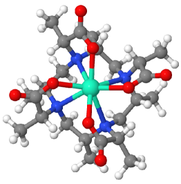
Figure 8: Optimized (B3LYP/ECP(Dy)/TZVP) structure of the [Dy(III)(M8mod)]^-1 complex.

The structure of the C₄-symmetric [Dy(III)(M8mod)]^-1 complex shown in Figure 8 was optimized with density functional theory (DFT) by means of the B3LYP functional Becke (1993); Lee, Yang, and Parr (1988) as implemented in Gaussian09 Frisch et al. . A Stuttgart/Dresden effective core potential with 55 core electrons Dolg, Stoll, and Preuss (1993) along with the corresponding valence TZVP Schäfer, Huber, and Ahlrichs (1994) basis set was employed for the Dy atom and, accordingly, a TZVP basis for the ligand atoms O, H, C and N. Subsequent four-component calculations were carried out within the framework of the DIRAC program DIR  employing (Abelian) C${}_{2}^{\ast}$ double group symmetry. We obtained the starting Kramers pair basis for the DMRG-CI calculations from an average-of-configuration Hartree-Fock calculation with nine electrons distributed in 14 spinors (corresponding to the $f^{9}$ open valence shell of Dy(III)) based on the four-component Dirac-Coulomb Hamiltonian. Uncontracted large-component basis sets of double-$\zeta$ quality (dubbed as DZ) were employed for Dy (dyall.v2z) Gomes, Dyall, and Visscher (2010) as well as for the ligand atoms (cc-pVDZ basis set Dunning Jr. (1989)). The small component basis set was generated using restricted kinetic balance. Starting from the optimized Hartree-Fock orbitals, we chose three different active orbital spaces for the subsequent DMRG-CI calculations, namely (i) a CAS(9,14) comprising all Dy $4f$ valence electrons and spinors, (ii) a CAS(27,32) adding the subvalence Dy $4p4s4d$ shell to the previous CAS and (iii) CAS(27,58) augmenting the preceding CAS with secondary spinors that have significant contributions from both Dy and ligand orbitals as determined from a Mulliken population analysis of the Hartree-Fock wave function. The current density and magnetization were obtained within VISUAL module of DIRAC and visualized by means of the pyngl-streamline program pyn . To this end, the VISUAL module had been extended to read a one-particle reduced density matrix in molecular spinor basis provided by QCMaquis which was subsequently transformed from molecular to atomic spinor basis to yield the density matrix D (cf. Eq.(50)) that constituted the starting point for the property density calculation. The DMRG-CI wave function optimizations and property density calculations employed a common gauge origin, placed at the center of mass. The visual integration was carried out within the respective planes specified in Section IV.3 by employing a $12$ bohr $\times$ $12$ bohr grid with the Dy(III) center placed at the (0,0,0) origin and 600 steps along each side corresponding to $600*600=360000$ integration points. Similar to the DMRG-CI setup for TlH, spinors for the MPS optimization were ordered according to orbital energies and pairing Kramers partners. The initial guess for the MPS in the starting sweep was based on random numbers (option init_state=default in QCMaquis). The sweep procedure was terminated after converge to 10^-6 Hartree was reached for a given number of renormalized states $m$.

IV.2 TlH

In order to assess the capabilities of our new four-component DMRG implementation, we compare absolute energies for the electronic $\Omega=0^{+}$ ground state of the thallium hydride molecule at different Tl-H internuclear distances to our benchmark data provided in Ref. 59.

Inspection of Table 3 reveals that the four-component DMRG-CI energy with $m=5000$ is, although being below the best variational CI energy (4c-CISDTQ in Table 3), still higher than the reference four-component CCSDTQ energy. We recall that DMRG is best suited for static-correlation problems, whereas TlH (close to equilibrium) is dominated by dynamic correlation as discussed on the basis of entanglement measures in Ref. 59. In addition, the latter claim is supported by a recent study of Shiozaki and Mizukami Shiozaki and Mizukami (2015) who considered ground-state spectroscopic properties of TlH based on a relativistic CASSCF reference wave function employing a minimal CAS(4,5) active space. They demonstrated that a subsequent treatment of dynamic-correlation contributions by means of multireference approaches such as CASPT2, NEVPT2 or internally-contracted MRCI+Q is sufficient to obtain excellent agreement with experimental reference data. Returning to our DMRG-CI results, Figure 9 illustrates the extrapolation of the DMRG-CI energy for an increasing number of renormalized states $m$ to the limit $E(m\rightarrow\infty)$ which provides an effective means to eliminate the truncation error. Following this procedure yields a best estimate of $\Delta E(m\rightarrow\infty)$ at R_e=1.872 Å as close as +0.1 mHartree to the four-component CCSDTQ reference energy.

Table 3: Total electronic energy differences $\Delta E$ (in mHartree) for different correlation approaches with respect to the four-component (4c-)CCSDTQ reference energies taken from Ref. 59. DMRG-CI results were obtained with an increasing number of renormalized block states $m$. For 4c-DMRG-CI[$m=5000$], energy differences are listed for five different internuclear distances $R_{\rm Tl-H}$ (in Å) given as subscripts.

Method	$\Delta E_{1.7720}$	$\Delta E_{1.8220}$	$\Delta E_{1.8720}$	$\Delta E_{1.9220}$	$\Delta E_{1.9720}$
4c-CISDTQ (Ref. 59)	2.57	2.60	2.63	2.66	2.70
4c-CCSDT (Ref. 59)	0.32	0.33	0.33	0.33	0.33
4c-CCSDT(Q) (Ref. 59)	-0.07	-0.06	-0.07	-0.07	-0.06
4c-DMRG-CI[$m=4500$] (Ref. 59)	-	-	2.57	-	-
4c-DMRG-CI[$m=500$]	-	-	28.16	-	-
4c-DMRG-CI[$m=1000$]	-	-	18.35	-	-
4c-DMRG-CI[$m=2000$]	-	-	8.44	-	-
4c-DMRG-CI[$m=4000$]	-	-	3.16	-	-
4c-DMRG-CI[$m=5000$]	2.53	2.49	2.51	2.45	2.51
4c-DMRG-CI[$m\rightarrow\infty$]	-	-	0.1	-	-

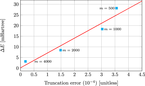
Figure 9: Extrapolation $\Delta E$ for $m\rightarrow\infty$ for the data obtained with QCMaquis. The difference to the reference CCSDTQ energy for the final extrapolated data is $0.1$ mHartree.

Finally, to achieve convergence in a DMRG-CI calculation usually requires a sufficient number of sweeps as can be seen in Figure 10. For example, the results obtained with $m=5000$ necessitated between 15 to 20 sweeps (depending on the internuclear Tl-H distance) to ensure a saturation of the (correlation) energy for the chosen $m$ value. Note that in the context of QCMaquis a total sweep corresponds to a combined left-to-right and right-to-left sweep as indicated in Figure 1.

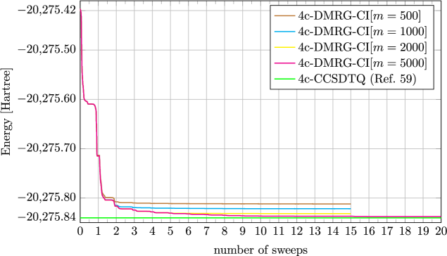
Figure 10: Energy convergence of a DMRG-CI calculation as a function of the number of sweeps performed for different values of $m$ at the experimental equilibrium internuclear distance R${}_{e}=1.872$ Å of the TlH molecule. For values of $m$ lower than $5000$, the sweeping procedure was terminated after fifteen iterations.

IV.3 Magnetic properties

In the previous section, we assessed the performance of our relativistic DMRG approach for the calculation of total energies in a small diatomic molecule by comparison to data obtained with our pilot implementation Knecht, Legeza, and Reiher (2014). In this section, we illustrate the potential of our new relativistic DMRG by examining selected magnetic properties of a Dy(III)-containing complex which goes beyond earlier capabilities. Because of symmetry restrictions , we consider in the following a model Dy(III) complex with the chelating octa-methyl DOTA (1,4,7,10 tetraaza-cyclododecane-tetraacetic acid) ligand denoted M8mod and shown in Figure 8 in contrast to the eight-fold, stereospecifically methylated DOTA derivatives dubbed as M8 that were employed in the work of Häussinger et al.Häussinger, Huang, and Grzesiek (2009). Owing to their high affinity towards (trivalent) lanthanides, DOTA complexes are ubiquitous in chelating lanthanides and are widely used for applications in magnetic resonance imaging Merbach, Helm, and Tóth (2013); Faulkner and Blackburn (2014), biomedical imaging Bünzli (2010); Stasiuk and Long (2013), biological nuclear magnetic resonance Wüthrich (1986); Piguet and Geraldes (2003); Pintacuda et al. (2007); Clore and Iwahara (2009); Bertini et al. (2017) and EPR-spectroscopy based distance measurements in proteins Pannier et al. (2000); Jeschke and Polyhach (2007); Jeschke (2012); Goldfarb (2014).

The chemistry of lanthanides is characterized in general — although a rich chemistry of Ln(II) complexes does exist as well, see for example Ref. 100 — by the $+3$ oxidation state omnipresent in the whole series as well as the compact nature of the $4f$ orbitals that exhibit an almost core-like character Cotton (2006). As a result, the $4f$ electrons contribute only to a limited extent to the chemical bonding which, in turn, leads to no strong preferences in coordination numbers and coordination polyhedra in lanthanide complexes of specific $4f$-shell configurations. Still, magnetic properties and electronic transitions of Ln complexes are sensitive to the coordination environment, though to a lesser extent than SO coupling and interelectronic repulsion effects, which makes them interesting target compounds for applications in magnetism and luminescence Cotton (2006).

We therefore chose in this work to study the (charge) current density j and magnetization m of the free Dy(III) ion in comparison with the [Dy(III)(M8mod)]^-1 complex shown in Figure 8. For this purpose, we carried out four-component DMRG-CI calculations with our newly developed relativistic DMRG model. By virtue of the expectation-value approach outlined in Section III.3, we obtained current densities and magnetizations for the bare Dy³⁺ ion and the [Dy(III)(M8mod)]^-1 complex in a real-space approach based on DMRG-CI wave functions with active orbital spaces of increasing size. As discussed in Ref. 75, a real-space approach allow us to visualize property densities without having to worry about orthonormality terms which would otherwise be needed in an analytical approach.

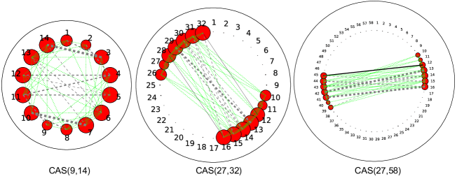
Figure 11: Entanglement diagrams for the electronic ground state of the [Dy(III)(M8mod)]^-1 complex obtained from 4c-DMRG-CI/DZ wave functions with increasing active orbital spaces. The area of the red circles indicates the magnitude of the single-orbital entropy $s_{p}(1)$. The line connecting two spinors $p$ and $q$ denotes their mutual information value $I_{pq}$ where darker (from green to black) and thicker lines correspond to an increasing value of the mutual information.

Figure 11 summarizes the single-orbital entropy $s_{p}$(1) Legeza and Sólyom (2003) for each spinor $p$ and the mutual information $I_{pq}$ Rissler, Noack, and White (2006); Legeza and Sólyom (2006) for spinor pairs $p,q$ calculated for the [Dy(III)(M8mod)]^-1 complex with increasing active orbital spaces. In all ring diagrams, spinors are ordered with all unbarred spinors first followed by their time-reversal partners. The diagram representation follows the scheme defined in Ref. 23: the area of the red circles assigned to each spinor $p$ is proportional to its single-orbital entropy $s_{p}(1)$ whereas the line connecting two spinors $p,q$ denotes their mutual information value $I_{pq}$. The direct connection between (spinor) entanglement and non-dynamical electron correlation — originally examined for spatial orbitals in a nonrelativistic framework Boguslawski et al. (2012) — provides a suitable means to analyze the active space in terms of non-dynamical electron correlation contributions originating from spinors exhibiting different character and/or interactions.

The entanglement diagrams in Figure 11  unequivocally illustrate that the valence electronic structure of the [Dy(III)(M8mod)]^-1 complex is predominantly governed by electron correlation within the partially filled $4f$ shell. For example, extending the active space beyond a CAS(9,14), corresponding to correlating all nine $4f$ electrons within the 14 $4f$ spinors, has virtually no effect neither on the single-orbital entropies $s_{p}(1)$ nor on the magnitude of the mutual information $I_{pq}$.

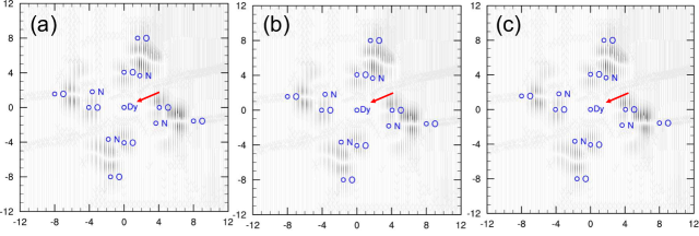
Figure 12: Comparison of the current density j obtained from DMRG-CI calculations with (a) CAS(9,14), (b) CAS(27,32), and (c) CAS(27,58) active orbital spaces. Visualization of j in the molecular plane containing the Dy(III) center in the (0,0,0) origin as indicated by a red arrow. Blue circles indicate the position of atomic centers where for better readability only the Dy(III) center as well as the oxygen and nitrogen centers of the chelating (M8mod)^4- ligand are shown. Line intensity is proportional to the norm of j.

Moreover, these conclusions are corroborated by the streamline plots of the current density j in the molecular plane containing the Dy(III) center in the (0,0,0) origin shown in Figure 12 as a function of increasing active orbital space size going from the smallest, CAS(9,14) (panel (a) in Figure 12) to the largest one, CAS(27,58) (panel (c) in Figure 12). The line intensities of the charge current density streamline plots are in close agreement both qualitatively and quantitatively for all three active spaces under consideration. Interestingly, the current density field appears to have sources and drains — the latter corresponding to a fading of the streamline intensity — that are in regions of space considerably distant from the central Dy(III) ion of the [Dy(III)(M8mod)]^-1 complex.

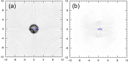
Figure 13: Streamline plots of the current density j (panel a) and magnetization m (panel b) in the plane comprising the Dy(III) center at the (0,0,0) origin. Data was obtained from a DMRG-CI/CAS(9,14) calculation of the bare Dy³⁺ ion. Line intensities are proportional to the norm of j and m, respectively.

Turning to streamline plots for the bare Dy³⁺ ion in Figure 13, this picture changes significantly for both the magnetization (right-hand side of Figure 13) and, particularly the current density field (left-hand side of Figure 13). We find in either case sizable streamline intensities spatially close to the core and valence region of the atomic center as could be expected for an open-shell $4f^{9}$ ion. Although putting the Dy(III) central ion into the crystal field of a chelating ligand such as M8mod did not seem to have a quantifiable influence on the local electronic ground-state structure of the resulting molecular [Dy(III)(M8mod)]^-1 complex (cf. Figure 11), ligand-field effects clearly induce a redistribution of the current density and magnetization, causing a density shift towards the ligand centers.

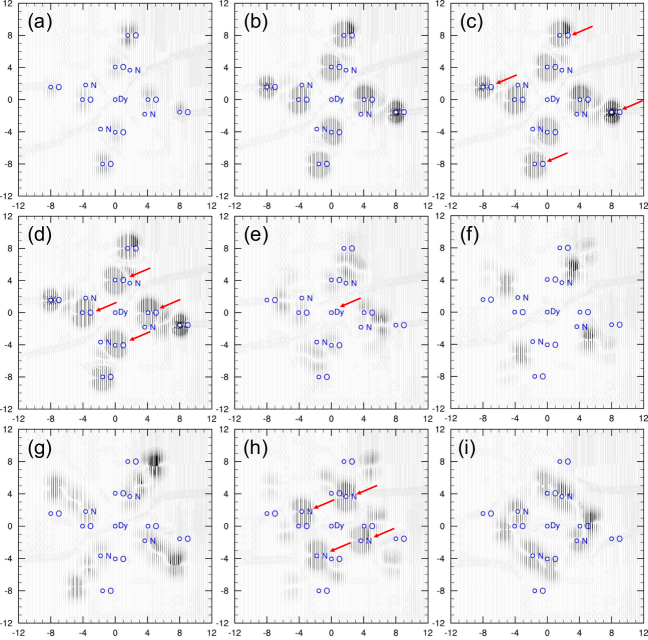
Figure 14: Current density j obtained from a DMRG-CI/CAS(27,32) calculation and visualized in different molecular planes from above (subfigures (a)-(d)) to below (subfigures (f)-(i)) the plane in $z$-direction which contains the Dy(III) center (subfigure (e)) in the (0,0,$z=0$) origin. Blue circles indicate the position of atomic centers. For better readability, only the Dy(III) center as well as the O and N centers of the chelating (M8mod)^4- ligand are shown. Red arrows indicate an integration plane containing the highlighted atomic center(s). Line intensities are proportional to the norm of j.

The latter is illustrated in Figures 14 and 15 for different molecular planes below and above the (0,0,$0$) plane comprising the Dy(III) center. Considering first the current density fields in Figure 14, we find stronger currents in particular in the planes containing the oxygen centers of the carboxylate groups of the chelating M8mod ligand compared to weaker ones within the plane spanned by the N atoms of the tetraaza-cyclododecane ring. By contrast, the situation is less clear for the magnetization, the spin-density analogue in a four-component relativistic framework, as can be seen from Figure 15. Notable line intensities of the magnetization streamline plots can be found above and below the Dy(III)-containing plane but they do not seem to coincide with particular atomic centers of the M8mod ligand.

In summary, by comparison to the bare Dy³⁺ ion our findings for the current density and magnetization of the [Dy(III)(M8mod)]^-1 complex substantiate the role of lanthanide chelating tags such as the Dy(III)-M8 complex presented first in Ref. 91 as a versatile paramagnetic label for the NMR spectroscopy of biomolecules (in solution). For example, lanthanide chelating tags play a particular role in the determination of structural parameters of a tagged biomolecule by virtue of (paramagnetic) NMR spectroscopic techniques Bleaney (1972). They give rise to (significant) pseudocontact shifts and sizable Fermi contact shifts Piguet and Geraldes (2003), both of which are together commonly referred to as hyperfine paramagnetic lanthanide induced shifts. These shifts originate from a large magnetic anisotropy of the paramagnetic center (pseudocontact shift) and from a non-zero spin-density at the probed (light-atom) nucleus caused by spin polarization through the spin-density of the paramagnetic central ion (Fermi contact shift) Kurland and McGarvey (1970), respectively. Concluding from the above findings for the current density and magnetization distributions for the modified [Dy(III)(M8mod)]^-1 complex both could be expected to be large in magnitude at nuclear centers distant from the paramagnetic Dy(III) center. These results are in line with the experimentally determined pseudocontact shifts based on paramagnetic NMR measurements employing the unmodified Dy(III)-M8 complex in Ref. 91.

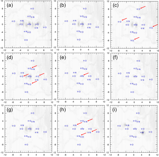
Figure 15: Magnetization m obtained from a DMRG-CI/CAS(27,32) calculation and visualized in different molecular planes from above (subfigures (a)-(d)) to below (subfigures (f)-(i)) the plane in $z$-direction which contains the Dy(III) center (subfigure (e)) in the (0,0,$z=0$) origin. Blue circles indicate the position of atomic centers. For better readability, only the Dy(III) center as well as the O and N centers of the chelating (M8mod)^4- ligand are shown. Red arrows indicate an integration plane containing the highlighted atomic center(s). Line intensities are proportional to the norm of m.

V Conclusions and Outlook

In this work we presented the formulation and efficient implementation of a genuine relativistic DMRG approach that exploits a matrix-product representation of the Hamiltonian as well as the wave function. To this end, we introduced a Kramers-paired spinor basis as well as double group symmetry into an existing nonrelativistic MPS/MPO-based DMRG algorithm. To demonstrate the suitability of our new relativistic DMRG model towards an unbiased exploration of the chemistry and properties of heavy element complexes, we considered two sample molecular systems. As a first example, we revisited the electron correlation problem in the electronic $\Omega=0^{+}$ ground state of the diatomic molecule TlH that became a standard test system for new relativistic correlated electronic structure electron approaches. With our relativistic DMRG model we were able to reach near full-CI accuracy for the absolute energy of the electronic ground state close to the equilibrium structure by considering an active orbital space as large as comprising 14 electrons in 94 spinors. Yet, to determine spectroscopic properties to high accuracy requires firstly to take into account dynamical electron correlation effects which can only be described to a certain extent in a DMRG model. Hence, we currently pursue the combination of our relativistic DMRG approach with (i) multireference perturbation theories such as CASPT2 Abe, Nakajima, and Hirao (2006); Kim and Lee (2014); Shiozaki and Mizukami (2015) and NEVPT2 Shiozaki and Mizukami (2015) as well as with (ii) a range-separated DFT ansatz Hedegård et al. (2015) that showed promising potential in a nonrelativistic framework. Secondly, orbital relaxation in the presence of SO coupling and explicit consideration of electron correlation is another crucial aspects striving for a high-accuracy computational model. In a recent work Ma et al. (2017), we demonstrated the robustness and efficiency of a second-order orbital optimization algorithm based on an MPS reference wave function. The formulation and implementation of its equivalent approach for a relativistic DMRG model is under way in our laboratory which will complement our locally available quasi-second-order DMRG-SCF implementation in Bagel bag  that was originally presented for a CI reference wave function Bates and Shiozaki (2015).

Magnetic properties offer a unique insight into the spectroscopy of open-shell molecules such as our second sample molecule, an $f^{9}$ [Dy(III)(M8mod)]^-1 complex. In this work, we investigated ligand-field effects on the magnetization and current density originating from the central Dy(III) ion by virtue of a real-space visualization of the density fields. In a graphical representation, we could illustrate an efficient spatial distribution of current density and magnetization originating from the paramagnetic Dy(III) center in direction to the ligand centers. The latter is a prerequisite for molecular complexes such as [Dy(III)(M8mod)]^-1 to serve as paramagnetic tags for biomolecules, making those available to paramagnetic NMR measurements. Consequently, an obvious extension of our expectation-value based property calculation approach for MPS wave functions will be the determination of first-order magnetic properties such as EPR g-tensors and hyperfine A-tensors. In a relativistic (four-component) framework, their calculation can be formulated as simple expectation values of well-defined one-electron operators Vad et al. (2013). Work in this direction is currently in progress.

References

- White (1992) S. R. White, Phys. Rev. Lett. 69, 2863 (1992).
- White (1993) S. R. White, Phys. Rev. B 48, 10345 (1993).
- Schollwöck (2005) U. Schollwöck, Rev. Mod. Phys. 77, 259 (2005).
- Schollwöck (2011) U. Schollwöck, Ann. Phys. 326, 96 (2011).
- Legeza et al. (2008) Ö. Legeza, R. M. Noack, J. Solyom, and L. Tincani, in Computational Many-Particle Physics, Lecture Notes in Physics, Vol. 739, edited by H. Fehske, R. Schneider, and A. Weisse (2008) pp. 653–664.
- Chan et al. (2008) G. K.-L. Chan, J. J. Dorando, D. Ghosh, J. Hachmann, E. Neuscamman, H. Wang, and T. Yanai, in Frontiers in Quantum Systems in Chemistry and Physics, Progress in Theoretical Chemistry and Physics, edited by S. Wilson, P. J. Grout, J. Maruani, G. Delgado-Barrio, and P. Piecuch (Springer Netherlands, 2008) pp. 49–65.
- Chan and Zgid (2009) G. K.-L. Chan and D. Zgid, Ann. Rep. Comp. Chem. 5, 149 (2009).
- Marti and Reiher (2010) K. H. Marti and M. Reiher, Z. Phys. Chem. 224, 583 (2010).
- Marti and Reiher (2011) K. H. Marti and M. Reiher, Phys. Chem. Chem. Phys. 13, 6750 (2011).
- Chan and Sharma (2011) G. K.-L. Chan and S. Sharma, Annu. Rev. Phys. Chem. 62, 465 (2011).
- Wouters and van Neck (2014) S. Wouters and D. van Neck, Eur. Phys. J. D 68, 272 (2014).
- Kurashige (2014) Y. Kurashige, Mol. Phys. 112, 1485 (2014).
- Yanai et al. (2015) T. Yanai, Y. Kurashige, W. Mizukami, J. Chalupsky, T. N. Lan, and M. Saitow, Int. J. Quantum Chem. 115, 283 (2015).
- Olivares-Amaya et al. (2015) R. Olivares-Amaya, W. Hu, N. Nakatani, S. Sharma, J. Yang, and G. K.-L. Chan, J. Chem. Phys. 142, 034102 (2015).
- Szalay et al. (2015) S. Szalay, M. Pfeffer, V. Murg, G. Barcza, F. Verstraete, R. Schneider, and Ö. Legeza, Int. J. Quantum Chem. 115, 1342 (2015).
- Knecht et al. (2016a) S. Knecht, E. D. Hedegaard, S. Keller, A. Kovyrshin, Y. Ma, A. Muolo, C. J. Stein, and M. Reiher, Chimia 70, 244 (2016a).
- Chan et al. (2016) G. K.-L. Chan, A. Keselman, N. Nakatani, Z. Li, and S. R. White, J. Chem. Phys. 145, 014102 (2016).
- Zgid and Nooijen (2008a) D. Zgid and M. Nooijen, J. Chem. Phys. 128, 144116 (2008a).
- Ghosh et al. (2008) D. Ghosh, J. Hachmann, T. Yanai, and G. K.-L. Chan, J. Chem. Phys. 128, 144117 (2008).
- Zgid and Nooijen (2008b) D. Zgid and M. Nooijen, J. Chem. Phys. 128, 144115 (2008b).
- Sun, Yang, and Chan (2017) Q. Sun, J. Yang, and G. K.-L. Chan, Chem. Phys. Lett. 683, 291 (2017).
- Ma et al. (2017) Y. Ma, S. Knecht, S. Keller, and M. Reiher, J. Chem. Theory Comput. 13, 2533 (2017).
- Stein and Reiher (2016) C. J. Stein and M. Reiher, J. Chem. Theory Comput. 12, 1760 (2016).
- Stein, von Burg, and Reiher (2016) C. J. Stein, V. von Burg, and M. Reiher, J. Chem. Theory Comput. 12, 3764 (2016).
- Stein and Reiher (2017) C. J. Stein and M. Reiher, Chimia 71, 170 (2017).
- Sayfutyarova et al. (2017) E. R. Sayfutyarova, Q. Sun, G. K.-L. Chan, and G. Knizia, J. Chem. Theory Comput. 13, 4063 (2017).
- Östlund and Rommer (1995) S. Östlund and S. Rommer, Phys. Rev. Lett. 75, 3537 (1995).
- Verstraete, Porras, and Cirac (2004) F. Verstraete, D. Porras, and J. I. Cirac, Phys. Rev. Lett. 93, 227205 (2004).
- Murg et al. (2010) V. Murg, F. Verstraete, Ö. Legeza, and R. M. Noack, Phys. Rev. B 82, 205105 (2010).
- Keller et al. (2015) S. Keller, M. Dolfi, M. Troyer, and M. Reiher, J. Chem. Phys. 143, 244118 (2015).
- Keller and Reiher (2016) S. Keller and M. Reiher, J. Chem. Phys. 144, 134101 (2016).
- (32) N. Nakatani, “MPSXX: MPS/MPO multi-linear library implemented in C++11, https://github.com/naokin/mpsxx.” .
- Dirac (1948) P. A. M. Dirac, The Principles of Quantum Mechanics, 3rd ed. (Oxford University Press, Oxford, 1948).
- Einstein (1905) A. Einstein, Z. Ann. Phys. 17, 891 (1905).
- Dirac (1928) P. A. M. Dirac, Proc. Roy. Soc. A 117, 610 (1928).
- Dyall and Fægri (2007) K. G. Dyall and K. Fægri, Introduction to Relativistic Quantum Chemistry (Oxford University Press, Oxford, 2007).
- Reiher and Wolf (2009) M. Reiher and A. Wolf, Relativistic Quantum Chemistry: The Fundamental Theory of Molecular Science (Wiley-VCH, Weinheim, 2009).
- Pyykkö (1988) P. Pyykkö, Chem. Rev. 88, 563 (1988).
- Saue (2011) T. Saue, ChemPhysChem 12, 3077 (2011).
- Autschbach (2012) J. Autschbach, J. Chem. Phys. 136, 150902 (2012).
- Cotton (2006) S. Cotton, Lanthanide and actinide chemistry (John Wiley & Sons, Ltd, 2006).
- Schwerdtfeger (2014) P. Schwerdtfeger, in The chemical bond: fundamental aspects of chemical bonding, edited by G. Frenking and S. Shaik (Wiley VCH, 2014) pp. 383–404.
- Demissie et al. (2016) T. B. Demissie, B. D. Garabato, K. Ruud, and P. M. Kozlowski, Angew. Chem. Int. Ed. 55, 11503 (2016).
- Gaggioli et al. (2016) C. A. Gaggioli, L. Belpassi, F. Tarantelli, D. Zuccaccia, J. N. Harvey, and P. Belanzoni, Chem. Sci. 7, 7034 (2016).
- Harriman (1978) J. E. Harriman, Theoretical Foundations of Electron Spin Resonance: Physical Chemistry: A Series of Monographs (Academic Press Inc., New York, 1978).
- Kaupp, Bühl, and Malkin (2004) M. Kaupp, M. Bühl, and V. G. Malkin, eds., Calculation of NMR and EPR parameters: theory and applications (Wiley-VCH, 2004).
- Jeschke and Polyhach (2007) G. Jeschke and Y. Polyhach, Phys. Chem. Chem. Phys. 9, 1895 (2007).
- Clore and Iwahara (2009) G. M. Clore and J. Iwahara, Chem. Rev. 109, 4108 (2009).
- Jeschke (2012) G. Jeschke, Ann. Rev. Phys. Chem. 63, 419 (2012).
- Goldfarb (2014) D. Goldfarb, Phys. Chem. Chem. Phys. 16, 9685 (2014).
- Bertini et al. (2017) I. Bertini, C. Luchinat, G. Parigi, and E. Ravera, in NMR of Paramagnetic Molecules, edited by I. Bertini, C. Luchinat, G. Parigi, and E. Ravera (Elsevier, Boston, 2017) 2nd ed., pp. 255–276.
- Szalay et al. (2012) P. G. Szalay, T. Müller, G. Gidofalvi, H. Lischka, and R. Shepard, Chem. Rev. 112, 108 (2012).
- Roca-Sanjuan, Aquilante, and Lindh (2012) D. Roca-Sanjuan, F. Aquilante, and R. Lindh, WIREs Comp. Mol. Sci. 2, 585 (2012).
- Malmqvist, Roos, and Schimmelpfennig (2002) P.-Å. Malmqvist, B. O. Roos, and B. Schimmelpfennig, Chem. Phys. Lett. 357, 230 (2002).
- Roemelt (2015) M. Roemelt, J. Chem. Phys. 143, 044112 (2015).
- Sayfutyarova and Chan (2016) E. R. Sayfutyarova and G. K.-L. Chan, J. Chem. Phys. 144, 234301 (2016).
- Knecht et al. (2016b) S. Knecht, S. Keller, J. Autschbach, and M. Reiher, J. Chem. Theory Comput. 12, 5881 (2016b).
- (58) B. Mussard and S. Sharma, Preprint on arXiv: 1710.00259.
- Knecht, Legeza, and Reiher (2014) S. Knecht, Ö. Legeza, and M. Reiher, J. Chem. Phys. 140, 041101 (2014).
- Keller (2016) S. Keller, Efficient Algorithms for the Matrix Product Operator Based Density Matrix Renormalization Group in Quantum Chemistry, Dissertation, Departement Chemie und Angewandte Biowissenschaften, ETH Zürich (2016).
- Keller and Reiher (2014) S. Keller and M. Reiher, Chimia 68, 200 (2014).
- Chan (2008) G. K.-L. Chan, Phys. Chem. Chem. Phys. 10, 3454 (2008).
- Jensen et al. (1996) H. J. Aa. Jensen, K. G. Dyall, T. Saue, and K. Fægri, J. Chem. Phys. 104, 4083 (1996).
- Thyssen, Fleig, and Jensen (2008) J. Thyssen, T. Fleig, and H. J. Aa. Jensen, J. Chem. Phys. 129, 034109 (2008).
- Kim and Lee (2013) I. Kim and Y. S. Lee, J. Chem. Phys 139, 134115 (2013).
- Bates and Shiozaki (2015) J. E. Bates and T. Shiozaki, J. Chem. Phys. 142, 044112 (2015).
- Aucar, Jensen, and Oddershede (1995) G. A. Aucar, H. J. Aa. Jensen, and J. Oddershede, Chem. Phys. Lett. 232, 47 (1995).
- Fleig, Olsen, and Marian (2001) T. Fleig, J. Olsen, and C. M. Marian, J. Chem. Phys. 114, 4775 (2001).
- Tinkham (1964) M. Tinkham, Group Theory and Quantum Mechanics (McGraw-Hill, New York, 1964).
- Saue and Jensen (1999) T. Saue and H. J. Aa. Jensen, J. Chem. Phys. 111, 6211 (1999).
- (71) DIRAC, a relativistic ab initio electronic structure program, Release DIRAC12 (2012), written by H. J. Aa. Jensen, R. Bast, T. Saue, and L. Visscher, with contributions from V. Bakken, K. G. Dyall, S. Dubillard, U. Ekström, E. Eliav, T. Enevoldsen, T. Fleig, O. Fossgaard, A. S. P. Gomes, T. Helgaker, J. K. Lærdahl, Y. S. Lee, J. Henriksson, M. Iliaš, Ch. R. Jacob, S. Knecht, S. Komorovský, O. Kullie, C. V. Larsen, H. S. Nataraj, P. Norman, G. Olejniczak, J. Olsen, Y. C. Park, J. K. Pedersen, M. Pernpointner, K. Ruud, P. Sałek, B. Schimmelpfennig, J. Sikkema, A. J. Thorvaldsen, J. Thyssen, J. van Stralen, S. Villaume, O. Visser, T. Winther, and S. Yamamoto (see http://www.diracprogram.org).
- Thyssen (2001) J. Thyssen, Development and Applications of Methods for Correlated Relativistic Calculations of Molecular Properties, Dissertation, Department of Chemistry and Physics, University of Southern Denmark (2001).
- Dolfi et al. (2014) M. Dolfi, B. Bauer, S. Keller, A. Kosenkov, T. Ewart, A. Kantian, T. Giamarchi, and M. Troyer, Comput. Phys. Commun. 185, 3430 (2014).
- Koster et al. (1963) G. F. Koster, J. O. Dimmock, R. G. Wheeler, and H. Statz, Properties of the thirty-two point groups (M.I.T Press, Cambridge, Massachusets, 1963).
- Bast (2008) R. Bast, Quantum chemistry beyond the charge density, Dissertation, University of Strasbourg (2008).
- Gordon (1928) W. Gordon, Z. Physik 50, 630 (1928).
- Sakurai (1967) J. Sakurai, Advanced Quantum Mechanics (Reading, MA: Addison-Wesley, 1967).
- Jacob and Reiher (2012) C. R. Jacob and M. Reiher, Int. J. Quantum Chem. 112, 3661 (2012).
- Dyall (2002) K. G. Dyall, Theor. Chem. Acc. 108, 335 (2002), erratum Theor. Chem. Acc. (2003) 109:284; revision Theor. Chem. Acc. (2006) 115:441.
- Dyall (2012) K. G. Dyall, Theor. Chem. Acc. 131, 1217 (2012).
- Dunning Jr. (1989) T. H. Dunning Jr., J. Chem. Phys. 90, 1007 (1989).
- Becke (1993) A. D. Becke, J. Chem. Phys. 98, 5648 (1993).
- Lee, Yang, and Parr (1988) C. Lee, W. Yang, and R. G. Parr, Phys. Rev. B 37, 785 (1988).
- (84) M. J. Frisch, G. W. Trucks, H. B. Schlegel, G. E. Scuseria, M. A. Robb, J. R. Cheeseman, G. Scalmani, V. Barone, B. Mennucci, G. A. Petersson, H. Nakatsuji, M. Caricato, X. Li, H. P. Hratchian, A. F. Izmaylov, J. Bloino, G. Zheng, J. L. Sonnenberg, M. Hada, M. Ehara, K. Toyota, R. Fukuda, J. Hasegawa, M. Ishida, T. Nakajima, Y. Honda, O. Kitao, H. Nakai, T. Vreven, J. A. Montgomery, Jr., J. E. Peralta, F. Ogliaro, M. Bearpark, J. J. Heyd, E. Brothers, K. N. Kudin, V. N. Staroverov, R. Kobayashi, J. Normand, K. Raghavachari, A. Rendell, J. C. Burant, S. S. Iyengar, J. Tomasi, M. Cossi, N. Rega, J. M. Millam, M. Klene, J. E. Knox, J. B. Cross, V. Bakken, C. Adamo, J. Jaramillo, R. Gomperts, R. E. Stratmann, O. Yazyev, A. J. Austin, R. Cammi, C. Pomelli, J. W. Ochterski, R. L. Martin, K. Morokuma, V. G. Zakrzewski, G. A. Voth, P. Salvador, J. J. Dannenberg, S. Dapprich, A. D. Daniels, B. Farkas, J. B. Foresman, J. V. Ortiz, J. Cioslowski, and D. J. Fox, “G09 Revision A.02,” Gaussian Inc. Wallingford CT 2009.
- Dolg, Stoll, and Preuss (1993) M. Dolg, H. Stoll, and H. Preuss, Theor. Chim. Acta 85, 441 (1993).
- Schäfer, Huber, and Ahlrichs (1994) A. Schäfer, C. Huber, and R. Ahlrichs, J. Chem. Phys. 100, 5829 (1994).
- Gomes, Dyall, and Visscher (2010) A. S. P. Gomes, K. G. Dyall, and L. Visscher, Theor. Chem. Acc. 127, 369 (2010).
- (88) Pyngl-streamline, a Python program written by R. Bast, https://github.com/bast/pyngl-streamline, accessed 08.12.2016.
- Shiozaki and Mizukami (2015) T. Shiozaki and W. Mizukami, J. Chem. Theory Comput. 11, 4733 (2015).
- Note (1) A bug in the DIRAC software package prevented us from obtaining correct two-electron integrals in molecular spinor basis for the C double group. By means of the Bagel program package bag , we could rule out an inconsistency in our QCMaquis implementation for the C double group.
- Häussinger, Huang, and Grzesiek (2009) D. Häussinger, J. Huang, and S. Grzesiek, J. Am. Chem. Soc. 131, 14761 (2009).
- Merbach, Helm, and Tóth (2013) A. Merbach, L. Helm, and É. Tóth, eds., The chemistry of contrast agents in medical magnetic resonance imaging, 2nd ed. (John Wiley & Sons, Ltd., 2013).
- Faulkner and Blackburn (2014) S. Faulkner and O. A. Blackburn, “The chemistry of lanthanide MRI contrast agents,” in The Chemistry of Molecular Imaging, edited by N. Long and W.-T. Wong (John Wiley & Sons, Inc, 2014) pp. 179–197.
- Bünzli (2010) J.-C. G. Bünzli, Chem. Rev. 110, 2729 (2010).
- Stasiuk and Long (2013) G. J. Stasiuk and N. J. Long, Chem. Comm. 49, 2732 (2013).
- Wüthrich (1986) K. Wüthrich, NMR of proteins and nucleic acids (John Wiley & Sons, New York, 1986).
- Piguet and Geraldes (2003) C. Piguet and C. F. Geraldes, in Handbook on the Physics and Chemistry of Rare Earths, Handbook on the Physics and Chemistry of Rare Earths, Vol. 33, edited by K. A. Gschneidner, J.-C. G. Bünzli, and V. K. Pecharsky (Elsevier, 2003) pp. 353–463.
- Pintacuda et al. (2007) G. Pintacuda, M. John, X.-C. Su, and G. Otting, Acc. Chem. Res. 40, 206 (2007).
- Pannier et al. (2000) M. Pannier, S. Veit, A. Godt, G. Jeschke, and H. W. Spiess, J. Magn. Reson. 142, 331 (2000).
- Szostak and Procter (2012) M. Szostak and D. J. Procter, Angew. Chem. Int. Ed. 51, 9238 (2012).
- Legeza and Sólyom (2003) O. Legeza and J. Sólyom, Phys. Rev. B 68, 195116 (2003).
- Rissler, Noack, and White (2006) J. Rissler, R. M. Noack, and S. R. White, Chem. Phys. 323, 519 (2006).
- Legeza and Sólyom (2006) O. Legeza and J. Sólyom, Phys. Rev. Lett. 96, 116401 (2006).
- Boguslawski et al. (2012) K. Boguslawski, P. Tecmer, Ö. Legeza, and M. Reiher, J. Phys. Chem. Lett. 3, 3129 (2012).
- Bleaney (1972) B. Bleaney, J. Magn. Reson. 8, 91 (1972).
- Kurland and McGarvey (1970) R. J. Kurland and B. R. McGarvey, J. Magn. Reson. 2, 286 (1970).
- Abe, Nakajima, and Hirao (2006) M. Abe, T. Nakajima, and K. Hirao, J. Chem. Phys. 125, 234110 (2006).
- Kim and Lee (2014) I. Kim and Y. S. Lee, J. Chem. Phys. 141, 164104 (2014).
- Hedegård et al. (2015) E. D. Hedegård, S. Knecht, J. S. Kielberg, H. J. A. Jensen, and M. Reiher, J. Chem. Phys. 142, 224108 (2015).
- (110) BAGEL, Brilliantly Advanced General Electronic-structure Library. http://www.nubakery.org under the GNU General Public License.
- Vad et al. (2013) M. S. Vad, M. N. Pedersen, A. Nørager, and H. J. Aa. Jensen, J. Chem. Phys. 138, 214106 (2013).