contents=
Coastal flood implications of 1.5 ∘C, 2.0 ∘C, and 2.5 ∘C temperature stabilization targets in the 21st and 22nd century
Abstract
Sea-level rise (SLR) is magnifying the frequency and severity of coastal flooding. The rate and amount of global mean sea-level (GMSL) rise is a function of the trajectory of global mean surface temperature (GMST). Therefore, temperature stabilization targets (e.g., 1.5 ∘C and 2.0 ∘C of warming above pre-industrial levels, as from the Paris Agreement) have important implications for coastal flood risk. Here, we assess differences in the return periods of coastal floods at a global network of tide gauges between scenarios that stabilize GMST warming at 1.5 ∘C, 2.0 ∘C, and 2.5 ∘C above pre-industrial levels. We employ probabilistic, localized SLR projections and long-term hourly tide gauge records to construct estimates of the return levels of current and future flood heights for the 21st and 22nd centuries. By 2100, under 1.5 ∘C, 2.0 ∘C, and 2.5 ∘C GMST stabilization, median GMSL is projected to rise 47 cm with a very likely range of 28–82 cm (90% probability), 55 cm (very likely 30–94 cm), and 58 cm (very likely 36–93 cm), respectively. As an independent comparison, a semi-empirical sea level model calibrated to temperature and GMSL over the past two millennia estimates median GMSL will rise within < 13% of these projections. By 2150, relative to the 2.0 ∘C scenario, GMST stabilization of 1.5 ∘C inundates roughly 5 million fewer inhabitants that currently occupy lands, including 40,000 fewer individuals currently residing in Small Island Developing States. Projected changes to the frequency of current 10-, 100-, and 500-year flood levels are quantified using flood amplification factors that incorporate uncertainty in both historical flood return periods and local SLR. Relative to a 2.0 ∘C scenario, the reduction in the amplification of the frequency of the 100-yr flood arising from a 1.5 ∘C GMST stabilization is greatest in the eastern United States and in Europe, with flood frequency amplification being reduced by about half.
1 Introduction
Coastal flooding is a hazard that threatens both life and property. The height of a coastal flood is determined by the combined height of the astronomical tide and storm surge (i.e., the storm tide) and the mean sea level at the time of the event. Rising mean sea levels are already magnifying the frequency and severity of coastal floods (Buchanan et al, 2017; Sweet and Park, 2014) and by the end of the century, coastal floods figure to be among the costliest impacts of climate change in some regions (Hsiang et al, 2017; Diaz, 2016). Sea-level rise (SLR) is expected to permanently inundate low-lying geographic areas (Marzeion and Levermann, 2014; Strauss et al, 2015), but these locations will first experience decreases in the return periods of flood events (e.g., Hunter, 2012; Sweet and Park, 2014).
The rate of global mean sea-level (GMSL) rise depends on the trajectory of global mean surface temperature (GMST; Rahmstorf, 2007; Kopp et al, 2016a; Vermeer and Rahmstorf, 2009), with the long-term committed amount of GMSL largely determined by the stabilized level of GMST (Levermann et al, 2013). Thus, the management of GMST has important implications for regulating future GMSL (Schaeffer et al, 2012), and consequently the frequency and severity of coastal floods. However, GMST stabilization does not imply stabilization of all climate variables. Under stabilized GMST, GSML is expected to continue to rise for centuries, due to the long residence time of anthropogenic CO2, the thermal inertia of the ocean, and the slow response of large ice sheets to forcing (Clark et al, 2016; Levermann et al, 2013; Held et al, 2010). For instance, Schaeffer et al (2012) found that a 2.0 ∘C GMST stabilization would lead to a GMSL rise (relative to 2000) of 0.8 m by 2100 and > 2.5 m by 2300, but if the GMST increase were held below 1.5 ∘C, GMSL rise at the end of the 23rd century would be limited to 1.5 m. These findings suggest that selection of climate policy goals could have critical long-term consequences for the impacts of future SLR and coastal floods (Clark et al, 2016).
The Paris Agreement seeks to stabilize GMST by limiting warming to “well below 2.0 ∘C above pre-industrial levels” and to further pursue efforts to “limit the temperature increase to 1.5 ∘C above pre-industrial levels” (UNFCCC, 2015a). However, a recent literature review under the United Nations Framework Convention on Climate Change (UNFCCC) found the notion that “up to 2.0 ∘C of warming is considered safe, is inadequate” and that “limiting global warming to below 1.5 ∘C would come with several advantages” (UNFCCC, 2015b). The advantages and disadvantages of each GMST target as they relate to coastal flooding have not been quantified. This is critical as > 625 million people currently live in low-elevation coastal zones, and population growth is expected in these areas (Neumann et al, 2015). Examining the short- and long-term flood hazard implications of 1.5 ∘C and 2.0 ∘C GMST stabilization scenarios, as others have recently done for other climate impacts (e.g. Schleussner et al, 2016a, b; Mitchell et al, 2017; Mohammed et al, 2017), may better inform the policy debate regarding the selection of GMST goals.
In this study, we employ probabilistic, localized SLR projections to assess differences in the frequency of extreme coastal floods across 1.5 ∘C, 2.0 ∘C, and 2.5 ∘C GMST stabilization scenarios at a global network of 194 tide gauges. We use long-term hourly tide gauge records and extreme value theory to estimate present and future return periods of flood events. We extend our analysis through the 22nd century to account for continuing SLR in order to inform multi-century planning and infrastructure investments. Lastly, we assess differences in the exposure of current populations to future SLR under 1.5 ∘C, 2.0 ∘C, and 2.5 ∘C GMST stabilizations.
Various approaches have been used to project GMSL under GMST targets. For instance, Jevrejeva et al (2016) estimate future local SLR under a GMST increase of 2 ∘C using an RCP8.5 GMST trajectory that passes through 2 ∘C of warming by mid-century, but this approach likely underestimates SLR relative to a scenario that achieves 2 ∘C GMST stabilization by 2100 as it neglects the time-lagged, integrated response of the ocean and cryosphere to warming (Clark et al, 2016). More generally, studies that condition future flood projections on the Representative Concentration Pathways (RCPs) may be insufficient for assessing the costs and benefits of climate policy scenarios, such as GMST stabilization targets (e.g., Section 13.7.2.2 of Church et al, 2013; Buchanan et al, 2017; Hunter, 2012; Tebaldi et al, 2012). The RCPs are designed to be representative of a range of emissions scenarios that result in prescribed anthropogenic radiative forcings by 2100 relative to pre-industrial conditions (e.g., 8.5 W for RCP8.5). They are not representative of a specific emissions trajectory, climate policy (e.g., GMST target), or socioeconomic and technological change (Moss et al, 2010; van Vuuren et al, 2011).
Semi-empirical sea level (SESL) models (Rahmstorf et al, 2012) can estimate future GMSL rise under various GMST scenarios (e.g., Schaeffer et al, 2012; Bittermann et al, in rev). Unlike their process-based counterparts (e.g., Kopp et al, 2014), SESL models do not explicitly model individual physical components of sea-level change. They are calibrated over a historical period using the observed statistical relationship between GMSL and a climate parameter (such as GMST). Assuming these relationships hold in the future, SESL models project the rate of GMSL change conditional upon a GMST pathway (e.g., Rahmstorf, 2007; Vermeer and Rahmstorf, 2009; Kopp et al, 2016a). However, SESL models do not produce estimates of local SLR, which are necessary for local risk assessment and adaptation planning because local SLR can substantially differ from the global mean (Milne et al, 2009).
2 Methods
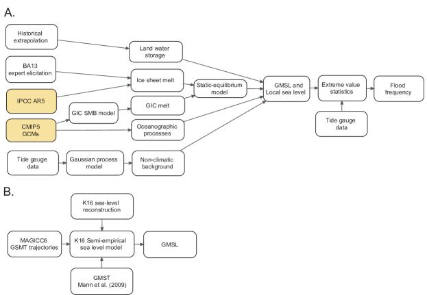
We project global and local sea level under 1.5 ∘C, 2.0 ∘C, and 2.5 ∘C GMST stabilization targets using the component-based, probabilistic, local sea level projection framework from Kopp et al (2014, henceforth K14). We compare the resulting GMSL projections to those from the semi-empirical sea level (SESL) model of Kopp et al (2016a). While SESL models cannot produce local projections of SLR, they can serve as a reference point for evaluating the consistency of process-based projections with historical temperature-GMSL relationships. The flow and sources of information used to construct the local SLR and GMSL projections using the K14 method is depicted in Fig. S-1A, while the flow of information used to generate the SESL projections is provided in Fig. S-1B. Local SLR projections from the K14 approach are combined with historical flood distributions to estimate future return periods of historical flood events (Fig. S-1A).
2.1 Component-based model approach: Global and local sea-level rise projections
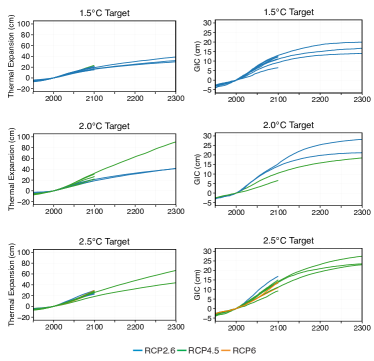
Global sea-level change does not occur uniformly. Dynamic ocean processes (Levermann et al, 2005), changes to temperature and salinity (i.e., steric processes), changes in the Earth’s rotation and gravitational field associated with water-mass redistribution (e.g., land-ice melt; Mitrovica et al, 2011), and glacial isostatic adjustment (GIA; Farrell and Clark, 1976) cause local sea levels to differ from the global mean. We model local sea level using the K14 framework, but make modifications to accommodate the stratification of Atmosphere-Ocean General Circulation Models (AOGCMs) and RCPs into groups that meet GMST stabilization targets (see Section 2.1.1). AOGCM output from the Coupled Model Intercomparison Project (CMIP) Phase 5 archive (Taylor et al, 2012) forced with the RCPs (to 2100) and their extensions (to 2300) are used for the following SLR components: global mean thermal expansion (TE), local ocean dynamics, and glacial ice contributions (GIC; Marzeion et al, 2012). Antarctic Ice Sheet (AIS) and the Greenland Ice Sheet (GIS) contributions are estimated using a combination of the Intergovernmental Panel on Climate Change’s (IPCC) Assessment Report 5 (AR5) projections of ice sheet dynamics and surface mass balance (SMB) (Table 13.5 in Church et al, 2013) and expert elicitation of total ice sheet mass loss from Bamber and Aspinall (2013). As in AR5, ice sheet SMB contributions are represented as being dependent on the forcing scenario, while ice sheet dynamics are not. Here, we use AR5’s AIS and GIS SMB contributions from RCP2.6 for both the 1.5 ∘C and 2.0 ∘C GMST scenarios and the RCP4.5 projection for the 2.5 ∘C GMST scenario (Table 13.5 in Church et al, 2013). A spatiotemporal Gaussian process regression model is used to estimate the long-term contribution from non-climatic factors such as tectonics and GIA. To generate probability distributions of global mean and local sea level at a global network of tide gauge sites (Table LABEL:Stab:tgauges) for each GMST scenario, we use 10,000 Latin hypercube samples of probability distributions of individual sea level component contributions.
2.1.1 Approximating Global Temperature Stabilization with RCPs
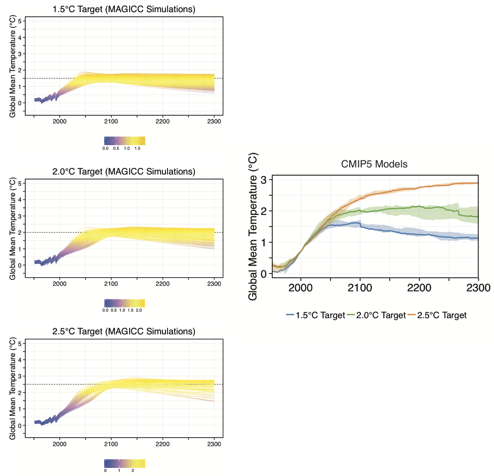
The RCP-driven experiments in the CMIP5 archive are not designed to inform the assessment of climate impacts from incremental temperature changes. As such, we construct alternative ensembles for 1.5 ∘C, 2.0 ∘C, and 2.5 ∘C scenarios using CMIP5 output according to each AOGCM’s 2100 GMST. Specifically, we create ensembles for 1.5 ∘C, 2.0 ∘C, and 2.5 ∘C scenarios with AOGCMs that have a 2100 GMST increase (19-yr running average) of 1.5 ∘C, 2.0 ∘C, and 2.5 ∘C ( 0.25 ∘C) relative to 1875–1900. Selection of the AOGCMs for each scenario ensemble are made irrespective of the AOGCM’s RCP forcing. For model outputs that end in 2100, we extrapolate 19-yr running average GMST to 2100 based on the 2070–2090 trend. While we chose 2100 as the determining year for which AOGCMs are selected for each ensemble, it should be noted that Article 2 of the UNFCCC (UNFCCC, 1992) does not require that GMST stabilization be achieved within a particular time frame. The Paris Agreement likewise does not specify a timeframe for GMST stabilization, though its goal of brining net greenhouse gas (GHG) emissions to zero in the second half of the 21st century implies a similar time frame for stabilization. We make the assumption that AOGCM outputs that end at 2100 either stay within the range of the target 0.25 ∘C or fall below by any amount (i.e., undershoot). For AOGCMs that have GSMT output available after 2100, only those that undershoot the target are retained. However, we make an exception to this rule for the 2.5 ∘C scenario ensemble in order to include AOGCMs for generating post-2100 projections. For RCP4.5 and RCP6, GMST stabilization should not occur before 2150, when greenhouse gas concentrations stabilize (Meinshausen et al, 2011b) and so SLR projections after 2100 may not be representative of conditions under true GMST stabilization.
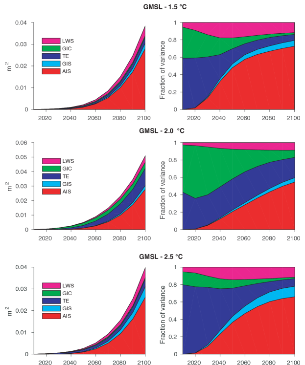
The GMST trajectories and GMSL contributions from TE and glacial ice from selected CMIP5 models that are binned into 1.5 ∘C, 2.0 ∘C, and 2.5 ∘C GMST categories are shown in Figs. 1 and S-2, respectively. For consistency with the K14 framework, which models 19-yr running averages of SLR relative to 2000, GMST is anomalized to 1991–2009 and then shifted upward by 0.72 ∘C to account for warming since 1875–1900 (Hansen et al, 2010; GISSTEMP Team, 2017). Table S-2 lists the AOGCMs employed in each GMST scenario ensemble and the sea-level components used. Given the paucity of CMIP5 output after 2100, the range of TE and GIC contributions to SLR in the 22nd century is likely underestimated relative to the 21st century.
2.2 Global mean sea-level rise projections from a semi-empirical sea level model
We generate estimates for GMSL for 2000–2100 using the SESL model from Kopp et al (2016a) driven with both GMST trajectories from CMIP5 models (Fig. 1) and GMST trajectories from the reduced-complexity climate model MAGICC6 (Meinshausen et al, 2011a, as employed in Rasmussen et al, 2016) for 2100 GMST targets of 1.5 ∘C, 2.0 ∘C, and 2.5 ∘C ( 0.25 ∘C) (Fig. S-3). The MAGICC6 GSMT trajectories are selected from all RCP-grouped projections using the same criteria as in Section 2.1.1. The SESL model is calibrated to the Common Era temperature reconstruction from Mann et al (2009) and the sea level reconstruction of Kopp et al (2016a). The historical statistical relationship between temperature and the rate of sea-level change is assumed to be constant; not included are nonlinear physical processes or critical threshold events that could substantially contribute to SLR, such as ice sheet collapse (Kopp et al, 2016b; Levermann et al, 2013). Threshold behavior is partially incorporated in the K14 framework through expert assessments of future ice sheet melt contributions (Bamber and Aspinall, 2013), which may be one reason why the K14 framework produces higher estimates in the upper tail of the SLR probability distribution for 2100.
2.3 Flood frequency estimation
2.3.1 Historic flood return levels
Extreme value theory is used with tide gauge observations to estimate the return levels of flood events of a given height, including those that occur less often, on average, than the length of the observational record (Coles, 2001b, a). Following Tebaldi et al (2012) and Buchanan et al (2016, 2017), we employ a generalized Pareto distribution (GPD) and a peaks-over-threshold approach to estimate the return periods of historical flood events at tide gauges. The GPD describes the probability of a given flood height conditional on an exceedance of the GPD threshold. Here, we use as the threshold the 99th percentile of daily maximum sea levels, which is generally both above the highest seasonal tide and balances the bias-variance trade-off in the GPD parameter estimation111If too low of a GPD threshold is chosen, more observations than those exclusively in the tail of the GPD distribution might end up being included in the parameter calculation, causing bias. If too high of a GPD threshold is chosen, then too few observations may be incorporated in the estimation of distribution parameters leading to greater variance, relative to a case that uses more observations. (Tebaldi et al, 2012). The number of annual exceedances of the GPD threshold is assumed to be Poisson distributed with mean . The GPD parameters are estimated using the method of maximum likelihood with tide gauge observations referenced to Mean Higher High Water (MHHW)222Here defined as the average level of high tide over the last 19-years in each tide gauge record, which is different from the current U.S. National Tidal Datum Epoch of 1983–2001. above the 99th percentile in each tide gauge’s record (see Supporting Information). Uncertainty in the GPD parameters is calculated from their covariance and is sampled using Latin hypercube sampling of a 1000 normally distributed GPD parameter pairs. For a given tide gauge, the annual expected number of exceedances of flood level is given by ():
| (1) |
where the shape parameter () governs the curvature and upward statistical limit of the flood return curve, the scale parameter () characterizes the variability in the exceedances caused by the combination of tides and storm surges, and the location parameter () is the threshold water-level above which return-levels are estimated with the GPD. Meteorological and hydrodynamic differences between sites gives rise to differences in the shape parameter (). Flood frequency distributions with > 0 are “heavy tailed”, due to a high frequency of extreme flood events (e.g., tropical and extra-tropical cyclones). Distributions with < 0 are “thin tailed” and have a statistical upper bound on extreme flood levels. Events that occur between and 182.6/year (i.e., exceeding MHHW half of the days per year) are modeled with a Gumbel distribution as they are outside of the domain of the GPD.
2.3.2 Flood frequency amplification factors
The amplification factor (AF) quantifies the increase in the expected frequency of historical flood events (e.g., the 100-yr flood) due to SLR (Buchanan et al, 2017; Hunter, 2012; Church et al, 2013). Due to variation in the local storm climate and hydrodynamics, the height of flood events are unique to each location (SI Fig. S-4). The calculation of the expected AF includes both the uncertainty in the estimates of the return periods of historical flood events and uncertainty in SLR projections. Following Buchanan et al (2017), we define the expected flood amplification factor for flood events with height as the ratio of the expected number of flood events after including uncertain SLR () to the historical expected number of flood events:
| (2) |
The flood AFs reported in this study should not be directly interpreted as changes in flood frequency. What constitutes a future flood event critically depends on the future level of coastal protection and adaptation efforts, both of which are unknown for most locations.
2.3.3 Assessment of population exposure
Following the methods used in Kopp et al (2017), we assess the current population exposed to permanent inundation from GMSL under each GMST stabilization scenario. We caution that this is not a measure of future population exposure, which will depend upon both population growth and the dynamic response of the population to rising sea levels, but is instead intended to provide a summary metric of the human significance of different sea levels. We use a 1-arcsec SRTM 3.0 digital elevation model from NASA (NASA JPL, 2013) that is referenced to local MHHW levels and this study’s local SLR projection grids. Projected inundation areas are intersected with current national population (Bright et al, 2011) and national boundary data (Hijmans et al, 2012). For each GMST target, the population exposed is assessed at the 50th, 5th, and 95th percentile local SLR projection. Further details are provided in the Supplementary Information of Kopp et al (2017).
3 Results
3.1 Global mean sea-level rise
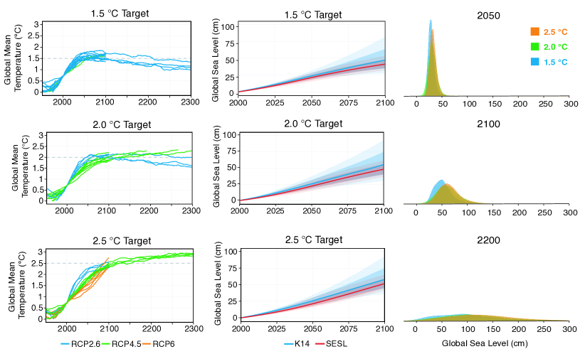
The GMSL projections for each GMST target from the K14 and SESL method are shown in Fig. 1 and are tabulated along with the component contributions in Table 1. For the K14 method, differences in median GMSL between 1.5 ∘C, 2.0 ∘C, and 2.5 ∘C GMST stabilization targets do not appear until after 2050, when the 1.5 ∘C scenario begins to separate from the 2.0 ∘C and 2.5 ∘C trajectories (Table 1). The median GMST trajectories diverge earlier, around 2030 (Fig. S-3). This is consistent with the early to mid-century divergence in the radiative forcing pathways and this study’s allocation of RCPs in the 1.5 ∘C (primarily RCP2.6), 2.0 ∘C (primarily RCP4.5), and 2.5 ∘C (primarily RCP4.5 and RCP6) scenarios (Table S-2). Median projections for 2100 GMSL under a 1.5 ∘C scenario are 47 cm, with a likely range (67% probability) of 35–63 cm. An additional 8–11 cm of median GMSL rise is found for the 2.0 ∘C and 2.5 ∘C GMST scenarios, 55 cm (likely 40–74 cm) and 58 cm (likely 44–75 cm), respectively. The sources of GMSL projection variance are shown in SI Fig. S-5. Using the same framework, Kopp et al (2014) found similar median 2100 GMSL projections under RCP2.6 and RCP4.5: 50 cm (likely 37–65 cm) and 59 cm (likely 45–77 cm), respectively.
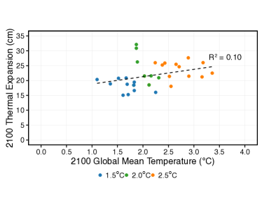
Despite being warmer by a half-degree, the 2.5 ∘C scenario largely overlaps the GMSL probability distribution for the 2.0 ∘C scenario (Fig. 1). For all GMST scenarios considered, TE contributes the most to median 2100 GMSL, and we find weak correlation ( = 0.10) between 2100 GMST and the corresponding TE contribution (Fig. S-6). The latter is due in part to variation in the transient climate response (TCR) and ocean heat uptake efficiency across CMIP5 models (Kuhlbrodt and Gregory, 2012; Raper et al, 2002). To test the sensitivity of model-RCP filtering to the choice of GMST stabilization, we additionally calculate GMSL under a 1.75 ∘C and 2.25 ∘C scenario. The median 2100 GMSL under the 1.75 ∘C scenario is 6 cm greater than the 1.5 ∘C scenario, and the 2.25 ∘C scenario is 1 cm less than the 2.0 ∘C scenario (Table S-3), suggesting that GMST scenarios that are primarily represented by only one RCP may be more sensitive to model filtering.
Agreement between central estimates from process-based and semi-empirical projections implies consistency with the observed statistical relationship between GMST and the rate of SLR used to calibrate the SESL model. Across scenarios, median 2100 GMSL projections from the SESL model driven with CMIP5 GMST trajectories are 6–7 cm lower than those from the K14 framework (Fig. 1 and Table 1), a difference that is less in magnitude to those between the K14 projections and Kopp et al (2016a) SESL projections for RCPs 2.6 and 4.5 (Kopp et al, 2016a, Table 2, showing median SESL projections of 38 cm and 51 cm for RCP2.6 and 4.5, vs. 50 and 59 cm for K14). The agreement between the processed-based and SESL projections is less when driven with the MAGICC GMST trajectories shown in SI Fig. S-3 (median projection differences of 8–11 cm; Table 1). Similarly, median estimates of 2100 GMSL for 1.5 ∘C and 2.0 ∘C scenarios from Schleussner et al (2016a) are 5–6 cm less than the projections using the K14 framework (Table 1). The SLR projections of Schleussner et al (2016a) are based on a method that scales SLR component contributions as a function of GMST and ocean heat uptake (Perrette et al, 2013).
3.2 Population inundation
Under the median projected GMSL for a 2.0 ∘C GMST stabilization, areas currently home to about 60 million people are at risk of being permanently submerged by 2150, including areas currently home to half a million inhabitants of United Nations defined Small Island Developing States (SIDS). By comparison, under the median projection for the 1.5 ∘C stabilization scenario, areas currently home to about 5 million people, including 40,000 in SID avoid inundation (Table 2). Aggregation of the SIDS can mask important risks. For instance, local SLR projections for 2150 under a 1.5 ∘C GMST stabilization place areas currently home to almost a quarter of the current population of the Marshall Islands at risk of being permanently submerged.
3.3 Amplification of flood events
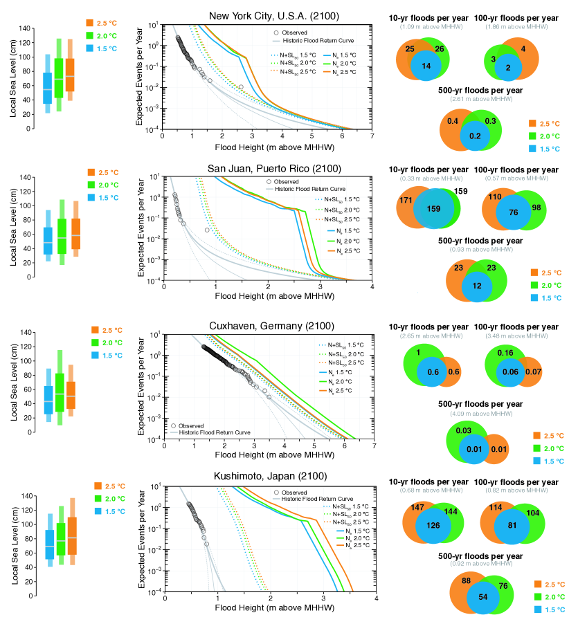
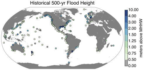
We assess the effects of different GMST stabilizations on coastal flooding by highlighting four cities: 1) New York, New York, USA 2) San Juan, Puerto Rico, USA 3) Cruxhaven, Lower Saxony, Germany, and 4) Kushimoto, Wakayama, Japan (Fig. 2). Estimates of the current 10-, 100-, and 500-yr flood (10%, 1%, 0.2% probability per year) and the future flood amplification factor (AF) for all sites are provided in SI Tables S-4 to S-6. Under a 2.0 ∘C GMST stabilization, the 2100 median local SLR for New York City is 69 cm, relative to 2000 (likely 43–98 cm). In Fig. 2, median local SLR shifts the expected historic flood return curve to the right [i.e., N(), the heavy grey curve, becomes N+SL50 2.0 ∘C, the dashed green curve] and increases the expected annual number of current 10-yr floods (a flood with a height of 1.09 m above MHHW) from 0.1/year to 10/year. However, when both the uncertainty in the GPD fit and the SLR projections are considered in the calculation of the projected future flood return curve (i.e., Ne 2.0 ∘C; the heavy green curve), the 10-yr flood amplification increases to 26/year (i.e., > 2/month). The discontinuities in the flood return curves demarcate the threshold where events are modeled with either a Gumbel distribution (from to 182.6 events per year) and with the GPD (Buchanan et al, 2016). GHG mitigation that stabilizes GMST at 1.5 ∘C reduces median local SLR at New York City to 55 cm (likely 35–78 cm), and reduces the number of expected annual 10-yr flood events by half (13/year). By 2150, the reduction in expected 10-yr flood events from the 2.0 ∘C to the 1.5 ∘C scenario is still roughly 50% (58/year vs. 97/year; Table S-4).
Sea-level rise will increase the frequency of all flood events, but some flood events will amplify more than others. While higher frequency events (i.e., the current 10-yr flood event) are expected to increase the most for New York City by 2100, San Juan is expected to experience greater increases in lower frequency floods (i.e., 500-yr events). Specifically, GMST stabilized at 2.0 ∘C is anticipated to produce 23 current 500-yr floods per year, on average (0.93 m above MHHW). If GMST warming is stabilized around 1.5 ∘C, the expected number of 500-yr floods is reduced by roughly half (12/year, on average). At higher levels of SLR, the most frequent flood events (e.g., the 10-yr flood) become driven by tidal events, as opposed to storm surges. By 2100, the 10-year flood is expected to occur almost every other day under all scenarios. For some sites, the AF for the 2.0 ∘C scenario may be greater than or equal to the AF for the 2.5 ∘C scenario. This can be observed for projections around the Baltic and North Sea where there is large uncertainty in the sign of the ocean dynamics contribution to local sea-level change between models. After 2100, the GMSL overlap between the 2.0 ∘C and 2.5 ∘C scenario projections leads to indistinguishable differences in flood projections for some locations (Fig. 1 and Table 1)
In Asia, under a 2.0 ∘C and 1.5 ∘C GMST stabilization, by 2100, Kushimoto is projected to have median local SLR of 77 cm (likely 57–102 cm) and 69 cm (likely 51–92 cm), respectively; increasing the current number of expected 100-yr floods for Kushimoto from 1/100 years, on average, to 104/year and 81/year, on average. Some locations are projected to have less local SLR compared to New York, San Juan, and Kushimoto, and therefore less flood amplification. By 2100, under both a 2.0 ∘C and 1.5 ∘C GMST stabilization, Cruxhaven is projected to have median local SLR increases of 54 cm (likely 29–83 cm) and 43 cm (likely 25–65 cm), respectively. Considering the entire projected probability distribution of SLR at Cruxhaven, the expected frequency of the current 500-yr flood event will become the future 100-yr flood.
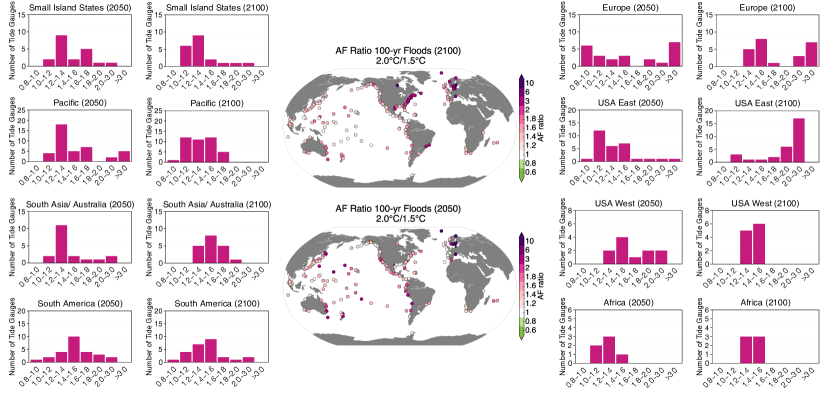
We assess regional differences in 100-yr flood amplification between 2.0 ∘C and 1.5 ∘C GMST stabilization by binning ratios of 2.0 ∘C/1.5 ∘C expected AFs for 2050 and 2100 (Fig. 3). Bins on the right side of each graph become filled when there are flood benefits at stations from 1.5 ∘C over 2.0 ∘C GMST stabilization, while bins on the left side of each graph become filled when there are little or no benefits at stations from 1.5 ∘C GMST over 2.0 ∘C GMST stabilization. At mid-century, only a few sites indicate benefits from a 1.5 ∘C GMST stabilization that are greater than 50% reductions in 100-yr flood frequency as GMSL trajectories between scenarios have not appreciably separated from one another (Table 1). However, by 2100, larger flood benefits of 1.5 ∘C GMST stabilization are expected in Europe and the East and Gulf Coasts of the United States (U.S.), where flood amplification is reduced by roughly half. We find minimal flood benefits from achieving a 1.5 ∘C GMST stabilization rather than a 2.0 ∘C GMST stabilization for the West Coast of the U.S., the Pacific, and Indian Ocean regions (Fig. 3).
4 Discussion and Conclusions
The Paris Agreement seeks to stabilize GMST by limiting warming to “well below 2.0 ∘C above pre-industrial levels”, but a recent literature review under the UNFCCC found the notion that “up to 2.0 ∘C of warming is considered safe, is inadequate” and that “limiting global warming to below 1.5 ∘C would come with several advantages” (UNFCCC, 2015b). However, given the geographic diversity of climate impacts from any GMST target, there cannot be an objective threshold that defines when all impacts reach unmanageable levels. The location-specific increases in the frequency of coastal floods is one such example. The selection of a GMST target has important implications for long-term GMSL rise and, consequently, coastal flooding. Assessing the distribution of impacts of incremental levels of warming on coastal flooding is of relevance to > 625 million people who currently reside in low-lying coastal areas (Neumann et al, 2015) and are vulnerable to current and future flood events. For countries without the economic and physical capacity to construct flood protection and flood-resilient infrastructure—including some recognized by the United Nations as Small Island Developing States—local SLR that results in permanent inundation and unmanageable flooding may threaten their existence (Wong et al, 2014; Diaz, 2016). The only feasible option for maintaining habitability for these locations may be the management of GMST through international climate accords, like the Paris Agreement, that govern the long-term committed rise in GMSL.
Only considering changes to the mean local sea level, we find that roughly 5 million fewer inhabitants currently reside in lands that will be permanently submerged by 2150 under a 1.5 ∘C GMST stabilization compared to that of the 2.0 ∘C case, including 40,000 fewer inhabitants of SIDS (Table 2). The effects of GMST stabilization on coastal flooding varies greatly by region and by return level (e.g., the 10-yr versus the 100-yr flood, ect.). Globally, for the current 100-yr flood, we find that by 2100, the Eastern and Gulf coasts of the U.S. and Europe could benefit the most from a 1.5 ∘C GMST stabilization relative to a 2.0 ∘C GMST stabilization, with flood frequency amplification being reduced by about half. However, while fractional reductions may appear substantial in some cases, small absolute differences may warrant similar coastal flood risk management responses. For instance, for New York City, we estimate that the difference in the expected number of current 100-yr floods per year (0.01 events per year, on average) between a 2.0 ∘C to a 1.5 ∘C GMST stabilization is only 3 times per year to 2 times per year, on average (Fig. 2).
While these data could be used in support of local probabilistic risk management strategies that intend to reduce current and future exposure and vulnerability to extreme flood events, some caveats should be highlighted. First, while our projections carry probabilities, the probabilities should be viewed in light of the characterization of the uncertainty of each sea level component. The true probability distribution of some sea level components may be imperfectly sampled. Second, changes to storm frequency and severity as well as effects from waves could significantly influence future flood events (e.g., Reed et al, 2015; Hatzikyriakou and Lin, 2017). In this study, wave effects are not considered, and we assume that the frequency of storm arrivals and their intensity will remain constant—and thus the Poisson and GPD scale and shape parameters. Modifications could be made to encompass changes in these parameters with time (Emanuel, 2013; Knutson et al, 2010). Lastly, these projections are for specific tide gauge locations and they may not be representative of the greater vicinity in which they are located.
The selection of the level at which to stabilize the GMST in the coming years will determine the committed amounts of future GMSL (Clark et al, 2016; Levermann et al, 2013). Our projected coastal flood impacts through the end of the 22nd century should be placed in the context of longer timeframes. Stabilization of GMST does not imply stabilization of GMSL. Regardless of the mitigation scenario chosen, GMSL rise due to TE is expected to continue for centuries to millennia. Additionally, some studies suggest that sustained GMST warming above given thresholds, including those as low as 2 ∘C, will lead to a near-complete loss of the GIS over a millennium or more (Church et al, 2013, section 13.4.3). Coincident with continued GMSL rise will be further increases in the frequency of current flood events and an increasing number of currently inhabited areas that will be permanently submerged. A comprehensive approach to managing coastal flood risks would take into account changes on these very long time frames.
Acknowledgements.
We thank XX anonymous reviewers and Carl-Friedrich Schleussner and colleagues at Climate Analytics (Berlin) for the helpful discussions. REK was supported in part by a grant from Rhodium Group (for whom he has previously worked as a consultant), as part of the Climate Impact Lab consortium and in part NSF grant ICER-1663807. We acknowledge the World Climate Research Programme’s Working Group on Coupled Modeling, which is responsible for CMIP, and we thank the climate modeling groups (listed in Supporting Information Table S-2) for producing and making available their model output. For CMIP, the U.S. Department of Energy’s Program for Climate Model Diagnosis and Intercomparison provides coordinating support and led development of software infrastructure in partnership with the Global Organization for Earth System Science Portals. Code for generating sea-level projections is available in the ProjectSL (https://github.com/bobkopp/ProjectSL), LocalizeSL (https://github.com/bobkopp/LocalizeSL), and SESL (https://github.com/bobkopp/SESL) repositories on Github. Code for generating flood projections is available in the XXXX (D.J. will upload) repository on Github. The statements, findings, conclusions, and recommendations are those of the authors and do not necessarily reflect the views of the funding agencies.References
- Bamber and Aspinall (2013) Bamber JL, Aspinall WP (2013) An expert judgement assessment of future sea level rise from the ice sheets. Nat Clim Chang 3(4):424–427, DOI 10.1038/nclimate1778, URL http://dx.doi.org/10.1038/nclimate1778
- Bittermann et al (in rev) Bittermann K, Rahmstorf S, Kopp RE, Kemp AC (in rev) Global mean sea-level rise in a world agreed upon in Paris. Environ Res Lett
- Bright et al (2011) Bright EA, Coleman PR, Rose AN, Urban ML (2011) LandScan 2010, Data Set
- Buchanan et al (2016) Buchanan MK, Kopp RE, Oppenheimer M, Tebaldi C (2016) Allowances for evolving coastal flood risk under uncertain local sea-level rise. Climatic Change 137(3):347–362, DOI 10.1007/s10584-016-1664-7, URL https://doi.org/10.1007/s10584-016-1664-7
- Buchanan et al (2017) Buchanan MK, Oppenheimer M, Kopp RE (2017) Amplification of flood frequencies with local sea level rise and emerging flood regimes. Environ Res Lett 064009(12):7
- Caldwell et al (2015) Caldwell PC, Merrifield MA, Thompson PR (2015) Sea level measured by tide gauges from global oceans — the Joint Archive for Sea Level holdings (NCEI Accession 0019568). NOAA National Centers for Environmental Information Dataset
- Church et al (2013) Church J, Clark P, Cazenave A, et al (2013) Sea Level Change. In: Stocker T, Qin D, Plattner GK, et al (eds) Clim. Chang. 2013 Phys. Sci. Basis. Contrib. Work. Gr. I to Fifth Assess. Rep. Intergov. Panel Clim. Chang., Cambridge University Press, Cambridge, UK and New York, NY, USA, chap 13
- Clark et al (2016) Clark PU, Shakun JD, Marcott SA, et al (2016) Consequences of twenty-first-century policy for multi-millennial climate and sea-level change. Nat Clim Chang 6(4):360–369, URL http://dx.doi.org/10.1038/nclimate2923http://10.0.4.14/nclimate2923http://www.nature.com/nclimate/journal/v6/n4/abs/nclimate2923.html{#}supplementary-information
- Coles (2001a) Coles S (2001a) Ch. 3: Classical Extreme Value Theory and Models. Lecture Notes in Control and Information Sciences, Springer, URL https://books.google.com/books?id=2nugUEaKqFEC
- Coles (2001b) Coles S (2001b) Ch. 4: Threshold Models. Lecture Notes in Control and Information Sciences, Springer, URL https://books.google.com/books?id=2nugUEaKqFEC
- Diaz (2016) Diaz DB (2016) Estimating global damages from sea level rise with the coastal impact and adaptation model (ciam). Climatic Change 137(1):143–156, DOI 10.1007/s10584-016-1675-4, URL https://doi.org/10.1007/s10584-016-1675-4
- Emanuel (2013) Emanuel KA (2013) Downscaling CMIP5 climate models shows increased tropical cyclone activity over the 21st century. Proc Natl Acad Sci U S A 110(30):12,219–24, DOI 10.1073/pnas.1301293110, URL http://www.pubmedcentral.nih.gov/articlerender.fcgi?artid=3725040{&}tool=pmcentrez{&}rendertype=abstract
- Farrell and Clark (1976) Farrell WE, Clark JA (1976) On postglacial sea level. Geophysical Journal of the Royal Astronomical Society 46(3):647–667, DOI 10.1111/j.1365-246X.1976.tb01252.x, URL http://dx.doi.org/10.1111/j.1365-246X.1976.tb01252.x
- GISSTEMP Team (2017) GISSTEMP Team (2017) GISS Surface Temperature Analysis (GISTEMP). URL https://data.giss.nasa.gov/gistemp/
- Hansen et al (2010) Hansen J, Ruedy R, Sato M, Lo K (2010) Global surface temperature change. Reviews of Geophysics 48(4):n/a–n/a, DOI 10.1029/2010RG000345, URL http://dx.doi.org/10.1029/2010RG000345, rG4004
- Hatzikyriakou and Lin (2017) Hatzikyriakou A, Lin N (2017) Simulating storm surge waves for structural vulnerability estimation and flood hazard mapping. Natural Hazards 89(2):939–962, DOI 10.1007/s11069-017-3001-5, URL https://doi.org/10.1007/s11069-017-3001-5
- Held et al (2010) Held IM, Winton M, Takahashi K, et al (2010) Probing the fast and slow components of global warming by returning abruptly to preindustrial forcing. Journal of Climate 23(9):2418–2427, DOI 10.1175/2009JCLI3466.1, URL https://doi.org/10.1175/2009JCLI3466.1, https://doi.org/10.1175/2009JCLI3466.1
- Hijmans et al (2012) Hijmans R, Kapoor J, Wieczorek J, et al (2012) GADM database of Global Administrative Areas 2.0, Data Set
- Hsiang et al (2017) Hsiang S, Kopp R, Jina A, et al (2017) Estimating economic damage from climate change in the united states. Science 356(6345):1362–1369, DOI 10.1126/science.aal4369, URL http://science.sciencemag.org/content/356/6345/1362, %****␣main.bbl␣Line␣125␣****http://science.sciencemag.org/content/356/6345/1362.full.pdf
- Hunter (2012) Hunter J (2012) A simple technique for estimating an allowance for uncertain sea-level rise. Clim Change 113(2):239–252, DOI 10.1007/s10584-011-0332-1
- Jevrejeva et al (2016) Jevrejeva S, Jackson LP, Riva REM, Grinsted A, Moore JC (2016) Coastal sea level rise with warming above 2 C. Proceedings of the National Academy of Sciences 113(47):13,342–13,347, DOI 10.1073/pnas.1605312113
- Knutson et al (2010) Knutson TR, McBride JL, Chan J, et al (2010) Tropical cyclones and climate change. DOI 10.1038/ngeo779
- Kopp et al (2014) Kopp RE, Horton RM, Little CM, et al (2014) Probabilistic 21st and 22nd century sea-level projections at a global network of tide-gauge sites. Earth’s Future pp 383–407, DOI 10.1002/2014EF000239.Abstract
- Kopp et al (2016a) Kopp RE, Bittermann K, Horton BP, et al (2016a) Temperature-driven global sea-level variability in the Common Era. Proceedings of the National Academy of Sciences 113(38)
- Kopp et al (2016b) Kopp RE, Shwom RL, Wagner G, Yuan J (2016b) Tipping elements and climate–economic shocks: Pathways toward integrated assessment. Earth’s Future 4(8):346–372, DOI 10.1002/2016EF000362, URL http://dx.doi.org/10.1002/2016EF000362, 2016EF000362
- Kopp et al (2017) Kopp RE, Deconto RM, Bader DA, et al (2017) Implications of ice-shelf hydrofracturing and ice-cliff collapse mechanisms for sea-level projections. arXiv pp 1–26, arXiv:1704.05597v1
- Kuhlbrodt and Gregory (2012) Kuhlbrodt T, Gregory JM (2012) Ocean heat uptake and its consequences for the magnitude of sea level rise and climate change. Geophys Res Lett 39(17):1–6, DOI 10.1029/2012GL052952
- Levermann et al (2005) Levermann A, Griesel A, Hofmann M, Montoya M, Rahmstorf S (2005) Dynamic sea level changes following changes in the thermohaline circulation. Climate Dynamics 24(4):347–354, DOI 10.1007/s00382-004-0505-y, URL https://doi.org/10.1007/s00382-004-0505-y
- Levermann et al (2013) Levermann A, Clark PU, Marzeion B, et al (2013) The multimillennial sea-level commitment of global warming. Proceedings of the National Academy of Sciences 110(34), DOI 10.1073/pnas.1219414110
- Mann et al (2009) Mann ME, Zhang Z, Rutherford S, et al (2009) Global signatures and dynamical origins of the little ice age and medieval climate anomaly. Science 326(5957):1256–1260, DOI 10.1126/science.1177303, URL http://science.sciencemag.org/content/326/5957/1256, http://science.sciencemag.org/content/326/5957/1256.full.pdf
- Marzeion and Levermann (2014) Marzeion B, Levermann A (2014) Loss of cultural world heritage and currently inhabited places to sea-level rise. Environmental Research Letters 9(3):034,001, URL http://stacks.iop.org/1748-9326/9/i=3/a=034001
- Marzeion et al (2012) Marzeion B, Jarosch aH, Hofer M (2012) Past and future sea-level change from the surface mass balance of glaciers. Cryosph 6(6):1295–1322, DOI 10.5194/tc-6-1295-2012, URL http://www.the-cryosphere.net/6/1295/2012/
- Meinshausen et al (2011a) Meinshausen M, Raper SCB, Wigley TML (2011a) Emulating coupled atmosphere-ocean and carbon cycle models with a simpler model, magicc6 – part 1: Model description and calibration. Atmospheric Chemistry and Physics 11(4):1417–1456, DOI 10.5194/acp-11-1417-2011, URL https://www.atmos-chem-phys.net/11/1417/2011/
- Meinshausen et al (2011b) Meinshausen M, Smith SJ, Calvin K, et al (2011b) The {RCP} greenhouse gas concentrations and their extensions from 1765 to 2300. Clim Change 109(1-2):213–241, DOI 10.1007/s10584-011-0156-z
- Milne et al (2009) Milne GA, Gehrels WR, Hughes CW, Tamisiea ME (2009) Identifying the causes of sea-level change. Nat Publ Gr 2(7):471–478, DOI 10.1038/ngeo544, URL http://dx.doi.org/10.1038/ngeo544
- Mitchell et al (2017) Mitchell D, AchutaRao K, Allen M, et al (2017) Half a degree additional warming, prognosis and projected impacts (happi): background and experimental design. Geoscientific Model Development 10(2):571–583, DOI 10.5194/gmd-10-571-2017, URL https://www.geosci-model-dev.net/10/571/2017/
- Mitrovica et al (2011) Mitrovica JX, Gomez N, Morrow E, et al (2011) On the robustness of predictions of sea level fingerprints. Geophys J Int (187):729–742, DOI 10.1111/j.1365-246X.2011.05090.x
- Mohammed et al (2017) Mohammed K, Islam AS, Islam GT, et al (2017) Extreme flows and water availability of the brahmaputra river under 1.5 and 2 °c global warming scenarios. Climatic Change DOI 10.1007/s10584-017-2073-2, URL https://doi.org/10.1007/s10584-017-2073-2
- Moss et al (2010) Moss RH, Edmonds Ja, Hibbard Ka, et al (2010) The next generation of scenarios for climate change research and assessment. Nature 463(7282):747–56, DOI 10.1038/nature08823, URL http://www.ncbi.nlm.nih.gov/pubmed/20148028
- NASA JPL (2013) NASA JPL (2013) NASA Shuttle Radar Topography Mission Global 1 arc second [Data set], NASA LP DAAC
- Neumann et al (2015) Neumann B, Vafeidis AT, Zimmermann J, Nicholls RJ (2015) Future coastal population growth and exposure to sea-level rise and coastal flooding - A global assessment. PLoS One 10(3), DOI 10.1371/journal.pone.0118571
- Perrette et al (2013) Perrette M, Landerer F, Riva R, Frieler K, Meinshausen M (2013) A scaling approach to project regional sea level rise and its uncertainties. Earth System Dynamics 4(1):11–29, DOI 10.5194/esd-4-11-2013, URL https://www.earth-syst-dynam.net/4/11/2013/
- Rahmstorf (2007) Rahmstorf S (2007) A semi-empirical approach to projecting future sea-level rise. Science 315(5810):368–370, DOI 10.1126/science.1135456, URL http://science.sciencemag.org/content/315/5810/368, http://science.sciencemag.org/content/315/5810/368.full.pdf
- Rahmstorf et al (2012) Rahmstorf S, Perrette M, Vermeer M (2012) Testing the robustness of semi-empirical sea level projections. Climate Dynamics 39(3):861–875, DOI 10.1007/s00382-011-1226-7, URL https://doi.org/10.1007/s00382-011-1226-7
- Raper et al (2002) Raper SCB, Gregory JM, Stouffer RJ (2002) The Role of Climate Sensitivity and Ocean Heat Uptake on AOGCM Transient Temperature Response. Journal of Climate 15(1):124–130, DOI 10.1175/1520-0442(2002)015<0124:TROCSA>2.0.CO;2, URL https://doi.org/10.1175/1520-0442(2002)015<0124:TROCSA>2.0.CO;2, https://doi.org/10.1175/1520-0442(2002)015<0124:TROCSA>2.0.CO;2
- Rasmussen et al (2016) Rasmussen DJ, Meinshausen M, Kopp RE (2016) Probability-weighted ensembles of u.s. county-level climate projections for climate risk analysis. Journal of Applied Meteorology and Climatology 55(10):2301–2322, DOI 10.1175/JAMC-D-15-0302.1, URL https://doi.org/10.1175/JAMC-D-15-0302.1, %****␣main.bbl␣Line␣300␣****https://doi.org/10.1175/JAMC-D-15-0302.1
- Reed et al (2015) Reed AJ, Mann ME, Emanuel KA, et al (2015) Increased threat of tropical cyclones and coastal flooding to new york city during the anthropogenic era. Proceedings of the National Academy of Sciences 112(41):12,610–12,615, DOI 10.1073/pnas.1513127112, URL http://www.pnas.org/content/112/41/12610.abstract, http://www.pnas.org/content/112/41/12610.full.pdf
- Schaeffer et al (2012) Schaeffer M, Hare W, Rahmstorf S, Vermeer M (2012) Long-term sea-level rise implied by 1.5 ∘C and 2 ∘C warming levels. Proceedings of the National Academy of Sciences 2(December 2012):867–870, DOI 10.1038/nclimate1584
- Schleussner et al (2016a) Schleussner Cf, Lissner TK, Fischer EM, et al (2016a) Differential climate impacts for policy-relevant limits to global warming: the case of 1.5 ∘C and 2 ∘C. Earth System Dynamics 7(2):327–351, DOI 10.5194/esd-7-327-2016
- Schleussner et al (2016b) Schleussner CF, Rogelj J, Schaeffer M, et al (2016b) Science and policy characteristics of the paris agreement temperature goal. Nature Clim Change 6(9):827–835, URL http://dx.doi.org/10.1038/nclimate3096
- Strauss et al (2015) Strauss BH, Kulp S, Levermann A (2015) Mapping Choices: Carbon, Climate, and Rising Seas, Our Global Legacy. Climate Central Research Report pp 1–38
- Sweet and Park (2014) Sweet WV, Park J (2014) From the extreme to the mean: Acceleration and tipping points of coastal inundation from sea level rise. Earth’s Future 2(12):579–600, DOI 10.1002/2014EF000272, URL http://dx.doi.org/10.1002/2014EF000272, 2014EF000272
- Taylor et al (2012) Taylor KE, Stouffer RJ, Meehl GA (2012) An overview of cmip5 and the experiment design. Bulletin of the American Meteorological Society 93(4):485–498, DOI 10.1175/BAMS-D-11-00094.1, URL https://doi.org/10.1175/BAMS-D-11-00094.1, https://doi.org/10.1175/BAMS-D-11-00094.1
- Tebaldi et al (2012) Tebaldi C, Strauss BH, Zervas CE (2012) Modelling sea level rise impacts on storm surges along US coasts. Environ Res Lett 7(1):014,032, DOI 10.1088/1748-9326/7/1/014032, URL http://stacks.iop.org/1748-9326/7/i=1/a=014032?key=crossref.99de1b370a3cea938a4cc90baa21719e
- UNFCCC (1992) UNFCCC (1992) The United Nations Framework Convention on Climate Change, UNFCCC
- UNFCCC (2015a) UNFCCC (2015a) Report of the Conference of the Parties on its twenty-first session, held in Paris from 30 November to 13 December 2015, UNFCCC
- UNFCCC (2015b) UNFCCC (2015b) Report on the structured expert dialogue on the 2013–2015 review, UNFCCC
- Vermeer and Rahmstorf (2009) Vermeer M, Rahmstorf S (2009) Global sea level linked to global temperature. Proceedings of the National Academy of Sciences 106(51):21,527–21,532, DOI 10.1073/pnas.0907765106, URL http://www.pnas.org/content/106/51/21527.abstract, http://www.pnas.org/content/106/51/21527.full.pdf
- van Vuuren et al (2011) van Vuuren DP, Edmonds J, Kainuma M, et al (2011) The representative concentration pathways: an overview. Climatic Change 109(1):5, DOI 10.1007/s10584-011-0148-z, URL https://doi.org/10.1007/s10584-011-0148-z
- Wong et al (2014) Wong PP, Losada IJ, Gattuso JP, et al (2014) Coastal systems and low-lying areas, Cambridge University Press, Cambridge, United Kingdom and New York, NY, USA, pp 361–409
5 Figures
| 1.5 ∘C | 2.0 ∘C | 2.5 ∘C | |||||||
| cm | 50 | 17–83 | 5–95 | 50 | 17–83 | 5–95 | 50 | 17–83 | 5–95 |
| 2100—Components | |||||||||
| AIS | 6 | -4–17 | -8–35 | 6 | -4–17 | -8–35 | 5 | -5–16 | -9–33 |
| GIS | 6 | 4–12 | 3–17 | 6 | 4–12 | 3–17 | 9 | 4–15 | 2–23 |
| TE | 19 | 14–23 | 10–27 | 25 | 16–34 | 9–42 | 26 | 20–31 | 16–35 |
| GIC | 11 | 8–13 | 6–15 | 12 | 7–16 | 4–21 | 13 | 11–15 | 9–17 |
| LWS | 5 | 3–7 | 2–8 | 5 | 3–7 | 2–8 | 5 | 3–7 | 2–8 |
| Total | 47 | 35–64 | 28–82 | 55 | 40–75 | 30–94 | 58 | 44–75 | 36–93 |
| Projections by year | |||||||||
| 2050 | 24 | 20–28 | 18–32 | 25 | 20–32 | 17–37 | 26 | 21–30 | 19–34 |
| 2070 | 33 | 27–41 | 23–49 | 37 | 28–48 | 23–58 | 38 | 31–47 | 27–55 |
| 2100 | 47 | 35–64 | 28–82 | 55 | 40–75 | 30–94 | 58 | 44–75 | 36–93 |
| 2150 | 68 | 41–106 | 28–150 | 89 | 54–134 | 35–178 | 86 | 53–128 | 35–169 |
| 2200 | 91 | 41–159 | 19–240 | 120 | 64–197 | 32–277 | 117 | 61–192 | 30–269 |
| Other projections for 2100 | |||||||||
| K161 | 38 | 33–43 | 30–47 | 45 | 39–52 | 35–58 | 54 | 47–62 | 42–68 |
| K162 | 41 | 36–48 | 32–53 | 48 | 41–56 | 36–62 | 51 | 45–59 | 41–65 |
| J16∗ | – | – | – | 22 | – | 15–33 | – | – | – |
| S16 | 41 | 29–53 | – | 50 | 36–65 | – | – | – | – |
| S12 | 77 | – | 54–99 | 80 | – | 56–105 | – | – | – |
| Other projections for 2200 | |||||||||
| S12 | 135 | – | 85–195 | 180 | – | 110–345 | – | – | – |
| 1 SESL model driven with MAGICC6 GMST trajectories shown in SI Fig. S-3 | |||||||||
| 2 SESL model driven with CMIP5 GMST trajectories shown in Fig. 1 | |||||||||
| Human population exposure under 2100 local SLR projections (millions) | ||||
| Region | Total Pop. | 1.5 ∘C | 2.0 ∘C | 2.5 ∘C |
| World | 6,836.42 | 45.88 (31.87–68.83) | 48.23 (31.99–78.38) | 50.27 (33.15–77.28) |
| China | 1,330.20 | 11.59 (5.87–20.22) | 12.53 (5.98–21.69) | 13.25 (6.12–22.93) |
| Vietnam | 89.55 | 6.55 (4.55–9.85) | 6.89 (4.58–10.44) | 7.14 (4.65–11.07) |
| Japan | 126.66 | 4.43 (3.82–5.54) | 4.59 (3.87–5.77) | 4.69 (3.88–6.10) |
| Netherlands | 16.78 | 4.71 (4.19–5.56) | 4.86 (4.18–5.88) | 4.84 (4.35–5.63) |
| Bangladesh | 156.13 | 2.81 (1.98–4.29) | 3.00 (2.06–4.66) | 3.09 (2.12–4.92) |
| SIDS | 62.08 | 0.40 (0.30–0.55) | 0.42 (0.30–0.63) | 0.43 (0.31–0.63) |
| Human population exposure under 2150 local SLR projections (millions) | ||||
| Region | Total Pop. | 1.5 ∘C | 2.0 ∘C | 2.5 ∘C |
| World | 6,836.42 | 55.49 (32.45–111.58) | 60.48 (32.83–133.88) | 61.95 (33.72–127.07) |
| China | 1,330.20 | 14.22 (5.72–30.54) | 16.38 (5.84–35.28) | 16.51 (5.69–36.73) |
| Vietnam | 89.55 | 7.53 (4.46–14.99) | 8.3 (4.50–16.61) | 8.27 (4.52–16.62) |
| Japan | 126.66 | 4.89 (3.82–5.54) | 5.3 (3.87–5.77) | 5.34 (3.88–6.10) |
| Netherlands | 16.78 | 5.06 (4.19–5.56) | 5.17 (4.18–5.88) | 5.26 (4.35–5.63) |
| Bangladesh | 156.13 | 4.43 (1.98–4.29) | 4.98 (2.06–4.66) | 4.98 (2.12–4.92) |
| SIDS | 62.08 | 0.46 (0.28–0.90) | 0.50 (0.29–1.11) | 0.51 (0.30–1.01) |
Supplementary Information
S-1 Preparation of tide gauge data for extreme value analysis
Tide gauge observations are prepared as the basis for extreme value analysis following the methods of Tebaldi et al (2012). First, daily maximum tide gauge values are calculated from the “Research Quality” hourly observations from the University of Hawaii Sea Level Center (retrieved from uhslc.soest.hawaii.edu, June 2017; Caldwell et al, 2015). Only tide gauge locations with record lengths 30 years and 80 percent data completion are considered. A list of tide gauges and their record lengths is provided in the Table LABEL:Stab:tgauges. The impact of day-to-day weather, astronomical tides and seasonal cycles on sea level is isolated by removing sea level change over the tide gauge record. Monthly-mean sea levels over the tide gauge record are used to linearly de-trend the daily maximum observations. Mean higher high water (MHHW) at each tide gauge is estimated using the average of the daily maximum tide gauge observations over the most recent 19-year period. While the MHHW calculation approach differs from the current U.S. standard (which is defined over the National Tidal Datum Epoch of 1983–2001), it is taken after de-trending of the time series and therefore should be close to stationary. Each de-trended tide gauge series is then referenced to its own MHHW level. Finally, at each tide gauge the daily observations above the 99th percentile are de-clustered to separate multiple observations made during the same extreme flood event and so that each observation is independent of one another. The 99th percentile is used as it is generally above the highest seasonal tide and it balances the bias-variance trade-off in the GPD parameter estimation. If too low of a GPD threshold is chosen, more observations than those exclusively in the tail of the GPD distribution might end up being included in the parameter calculation, causing bias. If too high of a GPD threshold is chosen, then too few observations may be incorporated in the estimation of distribution parameters leading to greater variance, relative to a case that uses more observations.
| Site | Country | Region | Lat | Lon | UHawaii ID | Start | End | Length (yrs) |
|---|---|---|---|---|---|---|---|---|
| Buenos Aires | Argentina | South America | -34.67 | -58.50 | 285a | 1905 | 1961 | 57 |
| Fort Denison | Australia | South Asia/ Australia | -33.90 | 151.32 | 333a | 1965 | 2015 | 51 |
| Bundaberg | Australia | South Asia/ Australia | -24.77 | 152.50 | 332a | 1984 | 2015 | 32 |
| Brisbane | Australia | South Asia/ Australia | -27.37 | 153.17 | 331a | 1984 | 2015 | 32 |
| Spring Bay | Australia | South Asia/ Australia | -42.67 | 148.07 | 335a | 1985 | 2015 | 31 |
| Townsville | Australia | South Asia/ Australia | -19.25 | 146.83 | 334a | 1984 | 2013 | 30 |
| Broome | Australia | South Asia/ Australia | -18.02 | 122.23 | 166a | 1986 | 2015 | 30 |
| Cocos | Australia | South Asia/ Australia | -12.12 | 96.97 | 171a | 1985 | 2015 | 31 |
| Darwin | Australia | South Asia/ Australia | -12.52 | 130.97 | 168a | 1984 | 2015 | 32 |
| Esperance | Australia | South Asia/ Australia | -33.90 | 122.02 | 176a | 1985 | 2015 | 31 |
| Fremantle | Australia | South Asia/ Australia | -32.05 | 115.73 | 175a | 1984 | 2015 | 32 |
| Cananeia | Brazil | South America | -25.02 | -48.00 | 281a | 1954 | 2006 | 53 |
| Ilha Fiscal, RJ | Brazil | South America | -23.02 | -43.30 | 280a | 1963 | 2012 | 50 |
| Victoria, BC | Canada | Canada | 48.50 | -123.40 | 543a | 1909 | 2014 | 106 |
| Prince Rupert | Canada | Canada | 54.32 | -130.38 | 540a | 1924 | 2014 | 91 |
| Tofino | Canada | Canada | 49.18 | -126.03 | 542a | 1930 | 2014 | 85 |
| St. John’s-A | Canada | Canada | 47.57 | -52.70 | 276a | 1952 | 1989 | 38 |
| Halifax | Canada | Canada | 44.67 | -63.58 | 275a | 1899 | 2014 | 116 |
| Churchill | Canada | Canada | 58.77 | -94.18 | 274a | 1961 | 2012 | 52 |
| Puerto Montt | Chile | South America | -41.50 | -73.07 | 684a | 1980 | 2014 | 35 |
| Juan Fernandez-B | Chile | South America | -33.67 | -78.95 | 021b | 1985 | 2014 | 30 |
| Antofagasta | Chile | South America | -23.68 | -70.45 | 080a | 1945 | 2014 | 70 |
| Easter-C | Chile | South America | -27.20 | -109.50 | 022c | 1970 | 2014 | 45 |
| Valparaiso | Chile | South America | -33.12 | -71.72 | 081a | 1944 | 2014 | 71 |
| Xiamen | China | Pacific | 24.45 | 118.07 | 376a | 1954 | 1997 | 44 |
| Buenaventura | Colombia | South America | 3.95 | -77.17 | 085a | 1953 | 2014 | 62 |
| Tumaco | Colombia | South America | 1.82 | -78.85 | 303a | 1951 | 2014 | 64 |
| Cartagena | Colombia | South America | 10.38 | -75.53 | 265a | 1951 | 1993 | 43 |
| Penrhyn | Cook Islands | SIDS | -9.07 | -158.08 | 024a | 1977 | 2015 | 39 |
| Quepos-A | Costa Rica | South America | 9.40 | -84.17 | 087a | 1961 | 1994 | 34 |
| Hornbaek | Denmark | Europe | 56.10 | 12.47 | 838a | 1891 | 2012 | 122 |
| Gedser | Denmark | Europe | 54.57 | 11.93 | 837a | 1891 | 2012 | 122 |
| Baltra-B | Ecuador | South America | -0.47 | -90.30 | 003b | 1985 | 2015 | 31 |
| Santa Cruz | Ecuador | South America | -0.80 | -90.43 | 030a | 1978 | 2015 | 38 |
| La Libertad | Ecuador | South America | -2.20 | -80.92 | 091a | 1949 | 2015 | 67 |
| Acajutla-A | El Salvador | South America | 13.58 | -89.83 | 082a | 1962 | 2001 | 40 |
| Chuuk | Fd. St. Micronesia | SIDS | 7.45 | 151.85 | 054a | 1956 | 1991 | 36 |
| Kapingamarangi | Fd. St. Micronesia | SIDS | 1.23 | 154.87 | 029a | 1978 | 2015 | 38 |
| Pohnpei-B | Fd. St. Micronesia | SIDS | 7.02 | 158.33 | 001b | 1974 | 2004 | 31 |
| Yap-B | Fd. St. Micronesia | SIDS | 9.58 | 138.23 | 008b | 1969 | 2015 | 47 |
| Suva-C | Fiji | SIDS | -18.27 | 178.52 | 018c | 1972 | 2015 | 44 |
| Noumea | France | Europe | -22.32 | 166.42 | 019a | 1967 | 2015 | 49 |
| Brest | France | Europe | 48.38 | -4.60 | 822a | 1846 | 2014 | 169 |
| Marseille | France | Europe | 43.38 | 5.38 | 824a | 1885 | 1988 | 104 |
| Rikitea | French Polynesia | SIDS | -23.20 | -134.98 | 016a | 1969 | 2015 | 47 |
| Papeete-B | French Polynesia | SIDS | -17.60 | -149.57 | 015b | 1975 | 2015 | 41 |
| Cuxhaven | Germany | Europe | 53.87 | 8.72 | 825a | 1917 | 2014 | 98 |
| Malin Head | Ireland | Europe | 55.37 | -7.33 | 834a | 1958 | 2001 | 44 |
| Hakodate | Japan | Pacific | 41.78 | 140.72 | 364a | 1964 | 2014 | 51 |
| Hamada | Japan | Pacific | 34.90 | 132.07 | 348a | 1984 | 2014 | 31 |
| Maisaka | Japan | Pacific | 34.68 | 137.62 | 356a | 1968 | 2014 | 47 |
| Ishigaki | Japan | Pacific | 24.33 | 124.15 | 365a | 1969 | 2014 | 46 |
| Naha | Japan | Pacific | 26.22 | 127.67 | 355a | 1966 | 2014 | 49 |
| Toyama | Japan | Pacific | 36.77 | 137.23 | 349a | 1967 | 2014 | 48 |
| Hosojima | Japan | Pacific | 32.42 | 131.68 | 358a | 1933 | 1975 | 43 |
| Kushiro | Japan | Pacific | 42.97 | 144.37 | 350a | 1963 | 2014 | 52 |
| Abashiri | Japan | Pacific | 44.02 | 144.28 | 347a | 1968 | 2014 | 47 |
| Mera | Japan | Pacific | 34.92 | 139.82 | 352a | 1965 | 2014 | 50 |
| Wakkanai | Japan | Pacific | 45.40 | 141.68 | 360a | 1967 | 2014 | 48 |
| Chichijima | Japan | Pacific | 27.10 | 142.18 | 047a | 1975 | 2014 | 40 |
| Nishinoomote | Japan | Pacific | 30.75 | 131.07 | 363a | 1965 | 2013 | 49 |
| Naze | Japan | Pacific | 28.52 | 129.60 | 359a | 1957 | 2013 | 57 |
| Hachinohe | Japan | Pacific | 40.53 | 141.53 | 375a | 1980 | 2011 | 32 |
| Miyakejima | Japan | Pacific | 34.07 | 139.62 | 357a | 1964 | 2013 | 50 |
| Nakano Shima | Japan | Pacific | 29.92 | 129.92 | 345a | 1984 | 2013 | 30 |
| Ofunato | Japan | Pacific | 39.02 | 141.75 | 351a | 1965 | 2014 | 50 |
| Nagasaki | Japan | Pacific | 32.73 | 129.87 | 362a | 1985 | 2014 | 30 |
| Aburatsu | Japan | Pacific | 31.58 | 131.42 | 354a | 1961 | 2014 | 54 |
| Kushimoto | Japan | Pacific | 33.48 | 135.77 | 353a | 1961 | 2014 | 54 |
| Cendering | Malaysia | South Asia/ Australia | 5.40 | 103.22 | 320a | 1984 | 2013 | 30 |
| Johor Baharu | Malaysia | South Asia/ Australia | 1.57 | 103.87 | 321a | 1983 | 2013 | 31 |
| Kuantan | Malaysia | South Asia/ Australia | 4.05 | 103.55 | 322a | 1983 | 2013 | 31 |
| Keling | Malaysia | South Asia/ Australia | 2.35 | 102.18 | 141a | 1984 | 2013 | 30 |
| Lumut | Malaysia | South Asia/ Australia | 4.30 | 100.73 | 143a | 1984 | 2013 | 30 |
| Kelang | Malaysia | South Asia/ Australia | 3.05 | 101.43 | 140a | 1983 | 2013 | 31 |
| Langkawi | Malaysia | South Asia/ Australia | 6.90 | 99.80 | 142a | 1985 | 2015 | 31 |
| Penang | Malaysia | South Asia/ Australia | 5.47 | 100.47 | 144a | 1984 | 2013 | 30 |
| Port Louis-C | Mauritius | SIDS | -20.20 | 57.60 | 103c | 1986 | 2015 | 30 |
| Rodrigues | Mauritius | SIDS | -19.68 | 63.43 | 105a | 1986 | 2015 | 30 |
| Manzanillo-A | Mexico | South America | 19.08 | -104.45 | 395a | 1953 | 1982 | 30 |
| Ensenada | Mexico | South America | 31.85 | -116.63 | 317a | 1956 | 1991 | 36 |
| Salina Cruz | Mexico | South America | 16.25 | -95.23 | 394a | 1952 | 1983 | 32 |
| Acapulco-A, Gro. | Mexico | South America | 16.90 | -100.02 | 316a | 1952 | 1995 | 44 |
| Cabo San Lucas | Mexico | South America | 23.00 | -109.98 | 034a | 1973 | 2002 | 30 |
| Guaymas | Mexico | South America | 27.93 | -110.90 | 397a | 1953 | 1986 | 34 |
| Saipan-B | N. Mariana Islands | SIDS | 15.32 | 145.82 | 028b | 1978 | 2015 | 38 |
| Marsden Point | New Zealand | South Asia/ Australia | -35.83 | 174.50 | 398a | 1975 | 2014 | 40 |
| Tauranga | New Zealand | South Asia/ Australia | -37.65 | 176.18 | 073a | 1984 | 2014 | 31 |
| Taranaki | New Zealand | South Asia/ Australia | -39.05 | 174.03 | 076a | 1984 | 2014 | 31 |
| Wellington | New Zealand | South Asia/ Australia | -41.28 | 174.78 | 071a | 1944 | 2014 | 71 |
| Tregde | Norway | Europe | 58.00 | 7.57 | 804a | 1927 | 2008 | 82 |
| Rorvik | Norway | Europe | 64.87 | 11.25 | 803a | 1969 | 2014 | 46 |
| Ny-Alesund | Norway | Europe | 78.93 | 11.95 | 823a | 1976 | 2014 | 39 |
| Vardo | Norway | Europe | 70.33 | 31.10 | 805a | 1979 | 2014 | 36 |
| Balboa | Panama | South America | 9.10 | -79.63 | 302a | 1907 | 2014 | 108 |
| Cristobal | Panama | South America | 9.40 | -80.05 | 266a | 1907 | 2014 | 108 |
| Rabaul | Papua New Guinea | SIDS | -4.20 | 152.25 | 010a | 1966 | 1997 | 32 |
| Lobos de Afuera | Peru | South America | -6.93 | -80.72 | 084a | 1982 | 2014 | 33 |
| Callao-B | Peru | South America | -12.08 | -77.17 | 093b | 1970 | 2015 | 46 |
| Legaspi | Philippines | Pacific | 13.25 | 123.83 | 371a | 1984 | 2015 | 32 |
| Manila | Philippines | Pacific | 14.60 | 120.98 | 370a | 1984 | 2015 | 32 |
| Cascais | Portugal | Europe | 38.77 | -9.42 | 209a | 1959 | 2005 | 47 |
| Funchal-B | Portugal | Europe | 32.73 | -17.03 | 218b | 1982 | 2013 | 32 |
| Kanton-B | Rep. of Kiribati | SIDS | -2.90 | -171.73 | 013b | 1972 | 2012 | 41 |
| Christmas-B | Rep. of Kiribati | SIDS | 2.12 | -157.52 | 011b | 1974 | 2015 | 42 |
| Majuro-A | Rep. of Marshall I | SIDS | 7.17 | 171.43 | 005a | 1968 | 1999 | 32 |
| Kwajalein | Rep. of Marshall I | SIDS | 8.73 | 167.73 | 055a | 1946 | 2014 | 69 |
| Malakal-B | Republic of Belau | SIDS | 7.45 | 134.58 | 007b | 1969 | 2015 | 47 |
| Kaohsiung | Republic of China | Pacific | 22.75 | 120.33 | 340a | 1980 | 2014 | 35 |
| Keelung | Republic of China | Pacific | 25.22 | 121.85 | 341a | 1980 | 2014 | 35 |
| Luderitz | South Africa | Africa | -26.65 | 15.15 | 702a | 1958 | 1995 | 38 |
| Saldahna Bay | South Africa | Africa | -33.02 | 17.95 | 703a | 1982 | 2011 | 30 |
| Simon’s Town | South Africa | Africa | -34.18 | 18.43 | 221a | 1959 | 1999 | 41 |
| Port Nolloth | South Africa | Africa | -29.25 | 16.87 | 701a | 1958 | 1997 | 40 |
| Port Elizabeth | South Africa | Africa | -34.05 | 25.75 | 184a | 1978 | 2014 | 37 |
| La Coruna | Spain | Europe | 43.37 | -8.40 | 830a | 1943 | 2013 | 71 |
| Ceuta | Spain | Europe | 35.90 | -5.32 | 207a | 1944 | 2013 | 70 |
| Vigo | Spain | Europe | 42.23 | -8.73 | 208a | 1943 | 1990 | 48 |
| Stockholm | Sweden | Europe | 59.40 | 18.22 | 826a | 1889 | 2014 | 126 |
| Goteborg-Torsh. | Sweden | Europe | 57.70 | 11.85 | 819a | 1967 | 2014 | 48 |
| Zanzibar | Tanzania | Africa | -6.20 | 39.25 | 151a | 1984 | 2015 | 32 |
| Ko Lak | Thailand | South Asia/ Australia | 11.90 | 99.82 | 328a | 1985 | 2015 | 31 |
| Stornoway | United Kingdom | Europe | 58.28 | -6.43 | 295a | 1976 | 2010 | 35 |
| Lerwick | United Kingdom | Europe | 60.20 | -1.20 | 293a | 1959 | 2010 | 52 |
| Faraday | United Kingdom | Europe | -65.25 | -64.27 | 700a | 1978 | 2013 | 36 |
| Gibraltar-A | United Kingdom | Europe | 36.13 | -5.35 | 289a | 1961 | 1992 | 32 |
| Bermuda-B | United Kingdom | Europe | 32.43 | -64.73 | 259b | 1985 | 2014 | 30 |
| Newlyn, Cornwall | United Kingdom | Europe | 50.12 | -5.62 | 294a | 1915 | 2010 | 96 |
| Seward-C, AK | USA | Canada | 60.15 | -149.52 | 560c | 1967 | 2014 | 48 |
| Ketchikan, AK | USA | Canada | 55.33 | -131.70 | 571a | 1937 | 2014 | 78 |
| Valdez, AK | USA | Canada | 61.20 | -146.47 | 562a | 1973 | 2014 | 42 |
| Yakutat, AK | USA | Canada | 59.68 | -139.75 | 570a | 1961 | 2014 | 54 |
| Seldovia, AK | USA | Canada | 59.50 | -151.75 | 561a | 1975 | 2014 | 40 |
| Sitka, AK | USA | Canada | 57.07 | -135.42 | 559a | 1938 | 2014 | 77 |
| Sand Point, AK | USA | Canada | 55.37 | -160.52 | 574a | 1973 | 2014 | 42 |
| Dutch Harbor-B, AK | USA | Canada | 54.00 | -166.57 | 041b | 1982 | 2014 | 33 |
| Cordova-B, AK | USA | Canada | 60.63 | -145.78 | 583b | 1964 | 2014 | 51 |
| Kodiak Isl., AK | USA | Canada | 57.87 | -152.62 | 039a | 1975 | 2014 | 40 |
| Adak, AK | USA | Canada | 51.98 | -176.77 | 040a | 1950 | 2014 | 65 |
| San Francisco, CA | USA | USA West | 37.87 | -122.60 | 551a | 1897 | 2014 | 118 |
| San Diego, CA | USA | USA West | 32.83 | -117.23 | 569a | 1906 | 2014 | 109 |
| Los Angeles, CA | USA | USA West | 33.75 | -118.32 | 567a | 1923 | 2014 | 92 |
| Crescent City, CA | USA | USA West | 41.85 | -124.18 | 556a | 1933 | 2014 | 82 |
| Monterey, CA | USA | USA West | 36.65 | -121.93 | 555a | 1973 | 2014 | 42 |
| Port San Luis, CA | USA | USA West | 35.27 | -120.85 | 565a | 1948 | 2014 | 67 |
| Santa Monica, CA | USA | USA West | 34.08 | -118.50 | 578a | 1973 | 2014 | 42 |
| La Jolla, CA | USA | USA West | 32.87 | -117.32 | 554a | 1924 | 2014 | 91 |
| New London, CT | USA | USA East | 41.40 | -72.12 | 744a | 1938 | 2014 | 77 |
| Lewes, DE | USA | USA East | 38.92 | -75.15 | 747a | 1957 | 2014 | 58 |
| Fernandina Beach, FL | USA | USA East | 30.72 | -81.47 | 240a | 1897 | 1930 | 34 |
| St. Petersburg, FL | USA | USA East | 27.85 | -82.72 | 759a | 1946 | 2014 | 69 |
| Pensacola, FL | USA | USA East | 30.43 | -87.33 | 762a | 1923 | 2014 | 92 |
| Mayport, FL | USA | USA East | 30.50 | -81.57 | 753a | 1928 | 2000 | 73 |
| Limetree Bay, FL | USA | USA East | 17.82 | -64.78 | 254a | 1982 | 2014 | 33 |
| Key West, FL | USA | USA East | 24.58 | -81.88 | 242a | 1913 | 2014 | 102 |
| Fort Pulaski, GA | USA | USA East | 32.03 | -80.92 | 752a | 1935 | 2014 | 80 |
| Hilo, HI | USA | Pacific | 19.73 | -155.07 | 060a | 1927 | 2014 | 88 |
| French Frigate, HI | USA | Pacific | 23.88 | -166.33 | 014a | 1974 | 2007 | 34 |
| Kahului, HI | USA | Pacific | 20.90 | -156.47 | 059a | 1950 | 2014 | 65 |
| Mokuoloe, HI | USA | Pacific | 21.43 | -157.80 | 061a | 1957 | 2014 | 58 |
| Honolulu-B, HI | USA | Pacific | 21.37 | -157.87 | 057b | 1905 | 2014 | 110 |
| Nawiliwili, HI | USA | Pacific | 21.97 | -159.35 | 058a | 1954 | 2014 | 61 |
| Grand Isle, LA | USA | USA East | 29.38 | -90.02 | 765a | 1980 | 2014 | 35 |
| Woods Hole, MA | USA | USA East | 41.58 | -70.72 | 742a | 1957 | 2014 | 58 |
| Nantucket, MA | USA | USA East | 41.30 | -70.22 | 743a | 1965 | 2014 | 50 |
| Boston, MA | USA | USA East | 42.40 | -71.07 | 741a | 1921 | 2014 | 94 |
| Portland, ME | USA | USA East | 43.72 | -70.37 | 252a | 1910 | 2014 | 105 |
| Eastport, ME | USA | USA East | 44.93 | -67.00 | 740a | 1929 | 2014 | 86 |
| Duck Pier, NC | USA | USA East | 36.18 | -75.87 | 260a | 1978 | 2014 | 37 |
| Wilmington, NC | USA | USA East | 34.32 | -77.98 | 750a | 1935 | 2014 | 80 |
| Atlantic City, NJ | USA | USA East | 39.40 | -74.43 | 264a | 1911 | 2014 | 104 |
| Cape May, NJ | USA | USA East | 38.98 | -75.05 | 746a | 1965 | 2014 | 50 |
| Montauk, NY | USA | USA East | 41.18 | -72.05 | 279a | 1959 | 2014 | 56 |
| New York, NY | USA | USA East | 40.70 | -74.15 | 745a | 1920 | 2014 | 95 |
| Charleston, OR | USA | USA West | 43.45 | -124.37 | 575a | 1978 | 2014 | 37 |
| South Beach, OR | USA | USA West | 44.70 | -124.13 | 592a | 1967 | 2014 | 48 |
| Astoria, OR | USA | USA West | 46.28 | -123.77 | 572a | 1925 | 2014 | 90 |
| Newport, RI | USA | USA East | 41.55 | -71.42 | 253a | 1930 | 2014 | 85 |
| Charleston, SC | USA | USA East | 32.92 | -80.00 | 261a | 1921 | 2014 | 94 |
| Rockport, TX | USA | USA East | 28.07 | -97.17 | 769a | 1944 | 2014 | 71 |
| Port Isabel, TX | USA | USA East | 26.15 | -97.35 | 772a | 1977 | 2014 | 38 |
| Chesapeake BBT, VA | USA | USA East | 36.97 | -76.23 | 749a | 1975 | 2014 | 40 |
| Neah Bay, WA | USA | USA East | 48.38 | -124.62 | 558a | 1934 | 2014 | 81 |
| Willapa Bay, WA | USA | USA East | 46.78 | -124.10 | 564a | 1972 | 2014 | 43 |
| Galveston, Pier 21, TX | USA | USA East | 29.40 | -94.88 | 775a | 1904 | 2014 | 111 |
| Galveston, P. Pier, TX | USA | USA East | 29.32 | -94.85 | 767a | 1957 | 2011 | 55 |
| Apra Harbor, Guam | USA Trust | Pacific | 13.43 | 144.65 | 053a | 1948 | 2014 | 67 |
| Wake | USA Trust | Pacific | 19.28 | 166.62 | 051a | 1950 | 2014 | 65 |
| Johnston | USA Trust | Pacific | 16.78 | -169.65 | 052a | 1947 | 2015 | 69 |
| Midway | USA Trust | Pacific | 28.22 | -177.37 | 050a | 1947 | 2014 | 68 |
| Pago Pago | USA Trust | Pacific | -14.28 | -170.68 | 056a | 1948 | 2014 | 67 |
| Charlotte Amalie, VI | USA Trust | SIDS | 18.35 | -64.95 | 255a | 1978 | 2014 | 37 |
| San Juan, PR | USA Trust | SIDS | 18.55 | -66.12 | 245a | 1977 | 2014 | 38 |
| Magueyes Island, PR | USA Trust | SIDS | 18.02 | -67.17 | 246a | 1965 | 2014 | 50 |
| 1.5 ∘C | ||||||
|---|---|---|---|---|---|---|
| Model | RCP | 2100 GMST (∘C) | GMST | Local Ocean | Thermal Expansion | GIC |
| bcc-csm1-1 | RCP 2.6 | 1.51 | 23 | 23 | 23 | 23 |
| BNU-ESM | RCP 2.6 | 1.62 | 21 | |||
| CCSM4 | RCP 2.6 | 1.45 | 23 | 23 | 21 | 21 |
| FIO-ESM | RCP 4.5 | 1.7 | 21 | 21 | ||
| GFDL-ESM2G | RCP 4.5 | 1.61 | 21 | 21 | ||
| HadGEM2-AO | RCP 2.6 | 1.74 | 21 | |||
| IPSL-CM5A-LR | RCP 2.6 | 1.74 | 23 | 23 | 23 | 23 |
| IPSL-CM5A-MR | RCP 2.6 | 1.6 | 21 | 21 | 21 | |
| MIROC5 | RCP 2.6 | 1.62 | 21 | 21 | ||
| MPI-ESM-LR | RCP 2.6 | 1.44 | 23 | 23 | 23 | 23 |
| MPI-ESM-MR | RCP 2.6 | 1.36 | 21 | 21 | 21 | |
| MRI-CGCM3 | RCP 2.6 | 1.72 | 21 | 21 | 21 | 21 |
| NorESM1-M | RCP 2.6 | 1.52 | 21 | 21 | 21 | 21 |
| NorESM1-ME | RCP 2.6 | 1.67 | 21 | 21 | 21 | |
| 2.0 ∘C | ||||||
| Model | RCP | 2100 GMST (∘C) | GMST | Local Ocean | Thermal Expansion | GIC |
| bcc-csm1-1 | RCP 4.5 | 2.21 | 23 | 23 | ||
| bcc-csm1-1-m | RCP 4.5 | 2.13 | 21 | 21 | 21 | |
| CanESM2 | RCP 2.6 | 2.17 | 23 | 23 | 23 | 23 |
| CESM1-BGC | RCP 4.5 | 2.24 | 21 | 21 | ||
| CESM1-CAM5 | RCP 2.6 | 2.13 | 23 | |||
| CSIRO-MK3-6-0 | RCP 2.6 | 2.04 | 21 | 21 | ||
| FGOALS-G2 | RCP 4.5 | 2.01 | 23 | |||
| GFDL-ESM2M | RCP 4.5 | 1.84 | 22 | 21 | 21 | |
| GISS-E2-H-CC | RCP 4.5 | 2.03 | 21 | |||
| GISS-E2-R | RCP 4.5 | 1.88 | 23 | 23 | 23 | 23 |
| GISS-E2-R-CC | RCP 4.5 | 1.87 | 21 | 21 | 21 | |
| HadGEM2-ES | RCP 2.6 | 1.97 | 23 | 23 | 23 | 23 |
| inmcm4 | RCP 4.5 | 2.04 | 21 | 21 | 21 | 21 |
| 2.5 ∘C | ||||||
| Model | RCP | 2100 GMST (∘C) | GMST | Local Ocean | Thermal Expansion | GIC |
| CCSM4 | RCP 4.5 | 2.31 | 23 | 23 | 21 | 21 |
| CNRM-CM5 | RCP 4.5 | 2.56 | 23 | 23 | 23 | 23 |
| FIO-ESM | RCP 6.0 | 2.34 | 21 | 21 | ||
| GFDL-CM3 | RCP 2.6 | 2.57 | 21 | 21 | 21 | 21 |
| GFDL-ESM2G | RCP 6.0 | 2.35 | 21 | 21 | 21 | |
| GFDL-ESM2M | RCP 6.0 | 2.53 | 21 | 21 | 21 | |
| GISS-E2-R | RCP 6.0 | 2.52 | 21 | 21 | 21 | 21 |
| IPSL-CM5B-LR | RCP 4.5 | 2.37 | 21 | 21 | ||
| MIROC-ESM | RCP 2.6 | 2.32 | 21 | 21 | 21 | 21 |
| MIROC-ESM-CHEM | RCP 2.6 | 2.42 | 21 | 21 | 21 | |
| MIROC5 | RCP 4.5 | 2.38 | 21 | 21 | 21 | |
| MPI-ESM-LR | RCP 4.5 | 2.38 | 23 | 23 | 23 | 23 |
| MPI-ESM-MR | RCP 4.5 | 2.39 | 21 | 21 | 21 | |
| MRI-CGCM3 | RCP 4.5 | 2.51 | 21 | 21 | 21 | |
| NorESM1-M | RCP 6.0 | 2.74 | 21 | 21 | 21 | 23 |
| NorESM1-M | RCP 4.5 | 2.33 | 23 | 23 | 21 | |
| NorESM1-ME | RCP 4.5 | 2.44 | 21 | 21 | 21 | |
| 21 = to 2100, 22 = to 2200, 23 = to 2300 | ||||||
| 1.75∘C | 2.25∘C | |||||
| cm | 50 | 17–83 | 5–95 | 50 | 17–83 | 5–95 |
| 2100—Components | ||||||
| AIS | 6 | -4–17 | -8–35 | 6 | -4–17 | -8–35 |
| GIS | 6 | 4–12 | 3–17 | 6 | 4–12 | 3–17 |
| TE | 21 | 12–30 | 6–37 | 23 | 20–27 | 17–30 |
| GIC | 12 | 8–15 | 6–17 | 13 | 9–16 | 6–20 |
| LWS | 5 | 3–7 | 2–8 | 5 | 3–7 | 2–8 |
| Total | 51 | 36–70 | 27–90 | 54 | 41–70 | 34–90 |
| Projections by year | ||||||
| 2050 | 25 | 20–30 | 17–34 | 25 | 21–30 | 18–34 |
| 2070 | 35 | 27–45 | 22–54 | 37 | 30–45 | 26–54 |
| 2100 | 51 | 36–70 | 27–90 | 54 | 41–70 | 34–90 |
| 2150 | 73 | 44–110 | 30–158 | 80 | 51–115 | 38–163 |
| 2200 | 98 | 46–164 | 21–252 | 107 | 55–172 | 30–260 |
| 10-yr Flood | |||||||||||
|---|---|---|---|---|---|---|---|---|---|---|---|
| 2050 | 2100 | 2150 | |||||||||
| Site | Region | Historical Height (m above MHHW) | AF 1.5∘C | AF 2.0∘C | AF 2.5∘C | AF 1.5∘C | AF 2.0∘C | AF 2.5∘C | AF 1.5∘C | AF 2.0∘C | AF 2.5∘C |
| Buenos Aires | Argentina | 2.15 | 2.1 | 2.3 | 2.3 | 8.1 | 12.6 | 13.8 | 57.3 | 100.5 | 95.5 |
| Fort Denison | Australia | 0.63 | 27.7 | 57.0 | 48.6 | 460.2 | 746.8 | 872.3 | 921.2 | 1286.3 | 1314.1 |
| Bundaberg | Australia | 0.91 | 15.7 | 23.8 | 21.5 | 232.9 | 397.4 | 460.0 | 717.8 | 1044.0 | 1030.3 |
| Brisbane | Australia | 0.65 | 44.6 | 72.3 | 63.6 | 570.1 | 870.8 | 948.4 | 1035.1 | 1351.8 | 1335.2 |
| Spring Bay | Australia | 0.57 | 46.2 | 83.1 | 98.6 | 704.6 | 1054.7 | 1143.0 | 1184.4 | 1464.5 | 1495.8 |
| Townsville | Australia | 1.18 | 10.6 | 14.0 | 13.2 | 112.1 | 176.1 | 221.0 | 470.9 | 748.1 | 734.8 |
| Broome | Australia | 2.27 | 11.1 | 12.0 | 13.2 | 39.2 | 49.7 | 56.3 | 125.7 | 187.1 | 176.6 |
| Cocos | Australia | 0.51 | 180.9 | 238.1 | 330.0 | 1304.3 | 1519.5 | 1575.3 | 1596.9 | 1658.1 | 1701.9 |
| Darwin | Australia | 1.53 | 18.5 | 20.0 | 21.9 | 88.7 | 121.7 | 142.1 | 322.4 | 492.4 | 478.1 |
| Esperance | Australia | 0.74 | 23.0 | 29.9 | 39.1 | 453.8 | 647.9 | 787.6 | 1012.8 | 1276.6 | 1312.8 |
| Fremantle | Australia | 0.74 | 22.5 | 30.4 | 39.3 | 469.0 | 696.8 | 842.2 | 1094.9 | 1335.6 | 1397.0 |
| Cananeia | Brazil | 0.96 | 19.3 | 28.6 | 26.8 | 418.1 | 681.5 | 755.7 | 1124.4 | 1311.9 | 1381.4 |
| Ilha Fiscal, RJ | Brazil | 0.83 | 15.1 | 22.9 | 21.0 | 335.6 | 585.5 | 652.1 | 921.1 | 1162.0 | 1208.7 |
| Victoria, BC | Canada | 0.91 | 4.7 | 5.9 | 7.0 | 101.1 | 131.5 | 183.4 | 370.7 | 576.4 | 542.8 |
| Prince Rupert | Canada | 1.56 | 4.8 | 5.2 | 5.4 | 38.7 | 43.8 | 50.7 | 154.7 | 165.1 | 208.8 |
| Tofino | Canada | 1.11 | 1.7 | 2.1 | 2.4 | 30.5 | 37.9 | 50.5 | 128.7 | 197.3 | 180.0 |
| St. John’s-A | Canada | 0.82 | 23.6 | 38.1 | 42.3 | 278.8 | 639.0 | 639.7 | 660.0 | 1075.5 | 1042.2 |
| Halifax | Canada | 0.84 | 34.5 | 48.1 | 57.2 | 437.5 | 842.7 | 911.5 | 965.0 | 1275.9 | 1392.6 |
| Churchill | Canada | 1.28 | 0.1 | 0.2 | 0.1 | 1.3 | 4.4 | 3.3 | 10.9 | 11.0 | 10.4 |
| Puerto Montt | Chile | 1.60 | 7.0 | 8.1 | 9.3 | 32.7 | 44.0 | 52.2 | 120.4 | 199.1 | 192.4 |
| Juan Fernandez-B | Chile | 0.52 | 32.3 | 44.5 | 53.1 | 579.7 | 759.3 | 911.6 | 1024.5 | 1239.3 | 1267.6 |
| Antofagasta | Chile | 0.48 | 20.1 | 38.1 | 43.1 | 453.7 | 684.4 | 807.5 | 862.0 | 1126.6 | 1157.5 |
| Easter-C | Chile | 0.59 | 11.2 | 18.4 | 18.8 | 510.5 | 699.6 | 822.7 | 1031.0 | 1249.9 | 1270.3 |
| Valparaiso | Chile | 0.53 | 13.4 | 22.2 | 24.4 | 262.2 | 452.5 | 551.9 | 658.9 | 939.8 | 964.9 |
| Xiamen | China | 1.43 | 6.3 | 7.3 | 8.7 | 71.2 | 91.9 | 129.0 | 313.5 | 489.1 | 502.5 |
| Buenaventura | Colombia | 1.06 | 22.2 | 27.1 | 27.5 | 194.8 | 293.9 | 342.2 | 638.9 | 910.9 | 894.4 |
| Tumaco | Colombia | 0.88 | 10.7 | 15.5 | 15.8 | 121.8 | 195.1 | 233.8 | 402.2 | 649.7 | 623.8 |
| Cartagena | Colombia | 0.25 | 1816.1 | 1747.8 | 1799.9 | 1825.7 | 1818.2 | 1826.0 | 1822.6 | 1808.5 | 1823.4 |
| Penrhyn | Cook Islands | 0.34 | 437.7 | 609.7 | 621.2 | 1549.6 | 1630.4 | 1672.8 | 1632.5 | 1688.9 | 1718.3 |
| Quepos-A | Costa Rica | 0.75 | 32.4 | 43.6 | 46.1 | 481.4 | 686.4 | 793.5 | 1019.8 | 1263.8 | 1274.2 |
| Hornbaek | Denmark | 1.25 | 4.3 | 42.8 | 3.8 | 37.5 | 287.1 | 45.7 | 171.1 | 347.4 | 190.8 |
| Gedser | Denmark | 1.29 | 3.8 | 23.4 | 3.4 | 40.4 | 228.1 | 51.0 | 201.0 | 315.9 | 237.0 |
| Baltra-B | Ecuador | 0.71 | 18.9 | 29.3 | 31.3 | 473.7 | 662.4 | 778.3 | 983.0 | 1224.1 | 1241.1 |
| Santa Cruz | Ecuador | 0.63 | 35.0 | 54.5 | 57.5 | 656.1 | 856.2 | 985.3 | 1119.2 | 1333.8 | 1353.8 |
| La Libertad | Ecuador | 0.74 | 51.1 | 73.6 | 75.6 | 954.1 | 1140.8 | 1276.9 | 1485.6 | 1587.5 | 1628.2 |
| Acajutla-A | El Salvador | 0.63 | 55.8 | 78.7 | 86.4 | 827.4 | 1037.5 | 1157.1 | 1305.1 | 1465.5 | 1489.2 |
| Chuuk | Fd. St. Micronesia | 0.40 | 202.5 | 274.0 | 298.8 | 1182.5 | 1390.0 | 1504.0 | 1417.4 | 1557.8 | 1596.3 |
| Kapingamarangi | Fd. St. Micronesia | 0.50 | 122.1 | 155.9 | 191.6 | 1176.0 | 1317.1 | 1451.6 | 1449.1 | 1582.2 | 1602.5 |
| Pohnpei-B | Fd. St. Micronesia | 0.51 | 127.3 | 166.3 | 175.5 | 1105.4 | 1310.7 | 1426.8 | 1418.6 | 1556.3 | 1587.8 |
| Yap-B | Fd. St. Micronesia | 0.54 | 70.9 | 96.5 | 109.9 | 951.8 | 1270.6 | 1369.6 | 1370.6 | 1527.1 | 1557.8 |
| Suva-C | Fiji | 0.51 | 269.0 | 317.3 | 333.3 | 1557.0 | 1513.7 | 1703.6 | 1731.1 | 1748.0 | 1720.1 |
| Noumea | France | 0.43 | 208.1 | 307.2 | 291.3 | 1242.8 | 1415.9 | 1550.6 | 1452.0 | 1611.9 | 1572.7 |
| Brest | France | 1.70 | 8.6 | 7.9 | 9.3 | 37.5 | 50.9 | 54.4 | 137.5 | 207.4 | 165.2 |
| Marseille | France | 0.68 | 10.2 | 125.7 | 15.1 | 262.5 | 570.1 | 411.9 | 812.3 | 754.0 | 1046.2 |
| Rikitea | French Polynesia | 0.31 | 532.3 | 751.2 | 761.0 | 1571.6 | 1664.8 | 1686.9 | 1625.9 | 1705.8 | 1673.2 |
| Papeete-B | French Polynesia | 0.31 | 637.9 | 885.9 | 878.7 | 1672.5 | 1704.1 | 1762.1 | 1709.3 | 1752.2 | 1733.2 |
| Cuxhaven | Germany | 2.65 | 2.1 | 2.1 | 2.0 | 5.7 | 12.4 | 6.3 | 36.4 | 34.7 | 34.0 |
| Malin Head | Ireland | 1.27 | 4.6 | 5.0 | 3.8 | 32.5 | 56.9 | 34.8 | 135.6 | 128.7 | 138.0 |
| Hakodate | Japan | 0.48 | 34.8 | 56.6 | 111.6 | 509.7 | 717.1 | 872.1 | 874.6 | 1123.6 | 1141.5 |
| Hamada | Japan | 0.63 | 27.3 | 42.3 | 80.3 | 668.0 | 896.5 | 1030.5 | 1114.0 | 1359.0 | 1331.2 |
| Maisaka | Japan | 0.77 | 1.8 | 2.2 | 3.8 | 74.2 | 109.8 | 179.4 | 284.6 | 478.8 | 522.3 |
| Ishigaki | Japan | 0.78 | 22.7 | 31.9 | 54.8 | 627.5 | 784.4 | 958.3 | 1126.2 | 1336.7 | 1359.5 |
| Naha | Japan | 0.71 | 40.0 | 57.7 | 105.2 | 748.2 | 912.5 | 1111.4 | 1192.0 | 1382.8 | 1416.4 |
| Toyama | Japan | 0.47 | 172.8 | 260.0 | 421.9 | 1308.0 | 1476.0 | 1520.1 | 1521.7 | 1649.8 | 1609.0 |
| Hosojima | Japan | 0.81 | 6.1 | 8.2 | 13.8 | 196.5 | 305.1 | 415.5 | 575.4 | 846.4 | 872.8 |
| Kushiro | Japan | 0.52 | 1570.4 | 1537.4 | 1584.6 | 1826.1 | 1823.6 | 1826.1 | 1826.1 | 1822.4 | 1826.0 |
| Abashiri | Japan | 0.64 | 38.7 | 80.8 | 93.6 | 664.3 | 905.2 | 1014.8 | 1164.8 | 1334.2 | 1363.9 |
| Mera | Japan | 0.60 | 155.1 | 207.1 | 311.1 | 1511.8 | 1613.3 | 1615.1 | 1724.9 | 1747.7 | 1710.9 |
| Wakkanai | Japan | 0.53 | 125.1 | 215.6 | 312.1 | 1265.2 | 1491.4 | 1488.6 | 1563.2 | 1678.3 | 1639.2 |
| Chichijima | Japan | 0.57 | 107.0 | 229.6 | 321.6 | 1199.0 | 1303.5 | 1488.0 | 1522.3 | 1600.6 | 1621.0 |
| Nishinoomote | Japan | 0.71 | 38.5 | 51.8 | 92.1 | 710.7 | 902.5 | 1044.5 | 1182.9 | 1408.9 | 1397.1 |
| Naze | Japan | 0.73 | 63.0 | 79.5 | 139.1 | 947.6 | 1092.5 | 1288.0 | 1361.0 | 1520.9 | 1540.4 |
| Hachinohe | Japan | 0.50 | 396.3 | 509.4 | 671.4 | 1651.2 | 1743.0 | 1729.8 | 1779.9 | 1783.0 | 1770.1 |
| Miyakejima | Japan | 0.87 | 157.1 | 173.4 | 242.2 | 1658.2 | 1711.9 | 1701.7 | 1813.4 | 1806.8 | 1798.8 |
| Nakano Shima | Japan | 0.74 | 51.0 | 65.7 | 114.1 | 858.9 | 1017.1 | 1156.1 | 1297.8 | 1484.3 | 1464.0 |
| Ofunato | Japan | 0.50 | 1221.5 | 1376.5 | 1306.1 | 1824.9 | 1823.2 | 1819.2 | 1825.7 | 1823.4 | 1822.1 |
| Nagasaki | Japan | 0.83 | 29.8 | 37.0 | 49.8 | 403.9 | 565.3 | 687.5 | 873.0 | 1144.7 | 1140.9 |
| Aburatsu | Japan | 0.82 | 10.3 | 13.9 | 25.9 | 350.3 | 509.0 | 646.2 | 859.3 | 1137.3 | 1148.4 |
| Kushimoto | Japan | 0.68 | 85.6 | 112.7 | 182.0 | 1254.5 | 1435.6 | 1473.5 | 1610.4 | 1686.8 | 1667.5 |
| Cendering | Malaysia | 0.90 | 13.7 | 16.9 | 19.4 | 232.5 | 351.1 | 445.7 | 654.3 | 889.4 | 886.5 |
| Johor Baharu | Malaysia | 0.81 | 34.1 | 40.8 | 46.9 | 432.4 | 589.6 | 717.2 | 898.4 | 1130.0 | 1133.7 |
| Kuantan | Malaysia | 0.96 | 18.4 | 21.8 | 24.6 | 253.0 | 370.3 | 468.0 | 706.0 | 940.5 | 938.7 |
| Keling | Malaysia | 0.65 | 40.1 | 49.9 | 58.5 | 518.0 | 679.3 | 817.1 | 917.1 | 1136.6 | 1139.2 |
| Lumut | Malaysia | 0.76 | 25.8 | 33.4 | 40.7 | 407.7 | 563.3 | 672.2 | 832.6 | 1068.3 | 1060.1 |
| Kelang | Malaysia | 1.22 | 12.5 | 13.9 | 15.7 | 114.1 | 156.9 | 204.5 | 425.4 | 599.5 | 588.5 |
| Langkawi | Malaysia | 0.83 | 29.0 | 35.9 | 42.9 | 322.8 | 461.0 | 562.0 | 736.7 | 973.8 | 964.1 |
| Penang | Malaysia | 0.72 | 46.8 | 59.6 | 72.8 | 535.6 | 713.5 | 827.1 | 954.6 | 1183.7 | 1178.7 |
| Port Louis-C | Mauritius | 0.41 | 109.6 | 177.3 | 271.5 | 1038.2 | 1329.3 | 1377.1 | 1320.4 | 1522.8 | 1542.5 |
| Rodrigues | Mauritius | 0.69 | 27.8 | 41.7 | 56.5 | 699.4 | 919.4 | 1050.9 | 1229.9 | 1454.6 | 1461.8 |
| Manzanillo-A | Mexico | 0.52 | 261.1 | 377.0 | 405.5 | 1670.8 | 1692.5 | 1737.9 | 1777.3 | 1760.1 | 1776.8 |
| Ensenada | Mexico | 0.65 | 53.6 | 78.9 | 84.2 | 694.5 | 921.0 | 1028.5 | 1226.9 | 1387.9 | 1419.1 |
| Salina Cruz | Mexico | 0.53 | 126.7 | 183.0 | 195.9 | 1313.4 | 1456.9 | 1552.7 | 1581.8 | 1655.7 | 1677.6 |
| Acapulco-A, Gro. | Mexico | 0.51 | 437.5 | 596.6 | 645.7 | 1800.8 | 1782.9 | 1807.9 | 1819.0 | 1799.7 | 1811.1 |
| Cabo San Lucas | Mexico | 0.59 | 49.2 | 73.9 | 76.7 | 724.4 | 947.7 | 1051.6 | 1195.4 | 1376.2 | 1395.0 |
| Guaymas | Mexico | 0.52 | 180.4 | 255.8 | 346.6 | 1577.0 | 1639.3 | 1663.3 | 1746.1 | 1742.9 | 1761.3 |
| Saipan-B | N. Mariana Islands | 0.44 | 125.2 | 186.6 | 209.5 | 1187.6 | 1311.4 | 1479.6 | 1398.0 | 1511.3 | 1584.4 |
| Marsden Point | New Zealand | 0.75 | 8.2 | 28.3 | 21.9 | 335.2 | 649.1 | 714.4 | 866.0 | 1254.1 | 1240.3 |
| Tauranga | New Zealand | 0.51 | 62.0 | 199.0 | 155.5 | 949.0 | 1307.1 | 1401.9 | 1272.3 | 1588.4 | 1596.8 |
| Taranaki | New Zealand | 1.10 | 3.8 | 7.8 | 6.5 | 88.7 | 194.1 | 214.7 | 439.4 | 757.9 | 733.1 |
| Wellington | New Zealand | 0.49 | 140.0 | 371.0 | 292.0 | 1311.5 | 1564.6 | 1626.5 | 1519.4 | 1720.1 | 1731.8 |
| Tregde | Norway | 0.77 | 11.5 | 17.5 | 9.8 | 112.7 | 215.3 | 143.5 | 350.2 | 407.7 | 450.3 |
| Rorvik | Norway | 1.15 | 1.5 | 3.2 | 1.7 | 17.2 | 36.0 | 22.3 | 77.5 | 86.1 | 76.7 |
| Ny-Alesund | Norway | 0.66 | 0.6 | 18.3 | 0.0 | 6.4 | 21.7 | 5.5 | 51.8 | 23.3 | 32.2 |
| Vardo | Norway | 1.03 | 3.7 | 15.1 | 5.7 | 37.5 | 111.6 | 64.6 | 135.6 | 234.3 | 184.0 |
| Balboa | Panama | 1.24 | 17.1 | 18.9 | 20.2 | 106.9 | 169.1 | 189.2 | 413.3 | 668.1 | 654.1 |
| Cristobal | Panama | 0.29 | 915.3 | 937.3 | 1108.2 | 1642.4 | 1711.5 | 1787.3 | 1635.2 | 1718.8 | 1750.3 |
| Rabaul | Papua New Guinea | 0.36 | 293.7 | 371.7 | 446.8 | 1360.1 | 1467.7 | 1597.7 | 1511.0 | 1628.0 | 1649.2 |
| Lobos de Afuera | Peru | 0.60 | 22.3 | 41.6 | 42.5 | 614.8 | 815.8 | 937.3 | 1060.7 | 1282.5 | 1300.7 |
| Callao-B | Peru | 0.46 | 29.3 | 57.1 | 66.4 | 687.4 | 885.0 | 1029.1 | 1054.0 | 1281.4 | 1307.1 |
| Legaspi | Philippines | 0.51 | 288.4 | 416.7 | 464.0 | 1616.7 | 1669.6 | 1742.3 | 1746.6 | 1740.0 | 1778.1 |
| Manila | Philippines | 0.69 | 424.1 | 546.3 | 613.1 | 1821.7 | 1815.2 | 1824.0 | 1825.5 | 1819.2 | 1825.5 |
| Cascais | Portugal | 0.93 | 17.1 | 15.4 | 21.6 | 156.3 | 236.4 | 313.1 | 556.8 | 790.4 | 802.6 |
| Funchal-B | Portugal | 0.64 | 93.9 | 84.8 | 129.6 | 739.2 | 930.6 | 1056.5 | 1170.9 | 1354.8 | 1459.1 |
| Kanton-B | Rep. of Kiribati | 0.43 | 122.4 | 191.0 | 199.9 | 1178.8 | 1349.5 | 1406.3 | 1409.2 | 1538.2 | 1577.7 |
| Christmas-B | Rep. of Kiribati | 0.42 | 209.0 | 322.3 | 333.7 | 1405.8 | 1490.2 | 1540.0 | 1541.7 | 1629.3 | 1659.5 |
| Majuro-A | Rep. of Marshall I | 0.60 | 110.2 | 139.8 | 137.8 | 1019.3 | 1207.0 | 1332.9 | 1396.9 | 1538.6 | 1577.0 |
| Kwajalein | Rep. of Marshall I | 0.51 | 222.8 | 274.2 | 283.6 | 1275.1 | 1460.0 | 1544.3 | 1533.4 | 1617.6 | 1669.9 |
| Malakal-B | Republic of Belau | 0.51 | 139.2 | 177.0 | 199.6 | 1069.9 | 1381.6 | 1450.4 | 1446.9 | 1590.3 | 1615.5 |
| Kaohsiung | Republic of China | 0.58 | 25.5 | 38.2 | 54.8 | 482.7 | 634.2 | 778.0 | 818.2 | 1049.7 | 1062.1 |
| Keelung | Republic of China | 0.67 | 24.0 | 36.9 | 68.0 | 774.9 | 945.7 | 1081.2 | 1174.9 | 1377.8 | 1376.7 |
| Luderitz | South Africa | 0.55 | 87.6 | 108.3 | 131.5 | 996.0 | 1228.5 | 1371.7 | 1350.3 | 1521.8 | 1581.8 |
| Saldahna Bay | South Africa | 0.60 | 79.4 | 93.1 | 113.5 | 825.8 | 1066.8 | 1184.7 | 1233.7 | 1438.8 | 1484.8 |
| Simon’s Town | South Africa | 0.62 | 75.5 | 90.1 | 111.3 | 934.4 | 1185.8 | 1309.2 | 1371.6 | 1542.0 | 1593.1 |
| Port Nolloth | South Africa | 0.64 | 57.8 | 69.8 | 75.9 | 750.8 | 1000.9 | 1142.8 | 1222.7 | 1441.6 | 1499.4 |
| Port Elizabeth | South Africa | 0.76 | 24.8 | 34.2 | 36.2 | 418.9 | 623.9 | 752.6 | 919.5 | 1211.9 | 1241.4 |
| La Coruna | Spain | 1.07 | 23.4 | 21.1 | 25.3 | 157.3 | 222.3 | 263.8 | 559.7 | 751.3 | 757.2 |
| Ceuta | Spain | 0.45 | 49.7 | 73.1 | 104.3 | 633.5 | 791.4 | 1005.8 | 1050.0 | 1264.2 | 1344.7 |
| Vigo | Spain | 1.10 | 17.6 | 16.2 | 20.4 | 144.5 | 209.2 | 254.6 | 543.4 | 750.8 | 748.4 |
| Stockholm | Sweden | 0.76 | 2.9 | 233.3 | 1.5 | 31.6 | 465.6 | 34.0 | 85.0 | 13.6 | 101.1 |
| Goteborg-Torsh. | Sweden | 1.12 | 2.9 | 14.6 | 2.5 | 28.8 | 162.2 | 33.2 | 124.8 | 188.2 | 129.7 |
| Zanzibar | Tanzania | 1.06 | 30.4 | 35.2 | 37.4 | 201.8 | 288.5 | 365.2 | 577.0 | 839.3 | 851.7 |
| Ko Lak | Thailand | 0.93 | 30.1 | 36.0 | 40.0 | 413.9 | 576.0 | 690.9 | 950.9 | 1178.7 | 1181.8 |
| Stornoway | United Kingdom | 1.39 | 7.0 | 6.5 | 6.1 | 35.7 | 49.6 | 38.3 | 141.8 | 123.8 | 139.4 |
| Lerwick | United Kingdom | 0.84 | 9.8 | 12.3 | 8.1 | 90.6 | 136.9 | 100.6 | 289.2 | 288.7 | 326.8 |
| Faraday | United Kingdom | 0.80 | 4.7 | 7.0 | 5.2 | 41.0 | 49.1 | 83.2 | 280.7 | 537.2 | 563.1 |
| Gibraltar-A | United Kingdom | 0.43 | 49.2 | 69.5 | 99.3 | 508.8 | 671.9 | 872.4 | 899.4 | 1135.4 | 1213.4 |
| Bermuda-B | United Kingdom | 0.53 | 72.5 | 91.2 | 121.9 | 927.8 | 1072.9 | 1152.6 | 1304.8 | 1454.9 | 1430.6 |
| Newlyn, Cornwall | United Kingdom | 1.24 | 15.8 | 15.9 | 15.4 | 87.2 | 129.1 | 111.0 | 304.6 | 375.9 | 408.1 |
| Seward-C, AK | USA | 1.28 | 0.5 | 0.8 | 0.6 | 9.7 | 12.6 | 11.2 | 51.0 | 58.3 | 59.5 |
| Ketchikan, AK | USA | 1.53 | 2.5 | 2.6 | 2.8 | 22.6 | 25.7 | 29.6 | 93.7 | 97.8 | 123.3 |
| Valdez, AK | USA | 1.29 | 0.2 | 0.4 | 0.3 | 6.2 | 8.6 | 6.9 | 35.1 | 42.6 | 40.5 |
| Yakutat, AK | USA | 1.26 | 0.0 | 0.0 | 0.0 | 2.7 | 3.6 | 3.0 | 16.4 | 16.1 | 16.6 |
| Seldovia, AK | USA | 1.79 | 0.1 | 0.1 | 0.1 | 0.7 | 0.8 | 0.7 | 10.7 | 11.3 | 10.9 |
| Sitka, AK | USA | 1.21 | 1.0 | 1.0 | 1.2 | 17.3 | 19.9 | 22.4 | 76.7 | 76.6 | 98.1 |
| Sand Point, AK | USA | 1.12 | 5.1 | 5.4 | 6.1 | 80.5 | 93.1 | 128.6 | 337.4 | 372.4 | 501.4 |
| Dutch Harbor-B, AK | USA | 0.72 | 0.8 | 1.0 | 1.3 | 39.5 | 48.7 | 64.9 | 133.0 | 148.3 | 204.6 |
| Cordova-B, AK | USA | 1.35 | 7.7 | 10.1 | 9.4 | 89.7 | 115.9 | 118.9 | 418.7 | 437.7 | 526.8 |
| Kodiak Isl., AK | USA | 1.09 | 0.1 | 0.1 | 0.2 | 3.9 | 4.4 | 4.3 | 20.1 | 19.9 | 20.9 |
| Adak, AK | USA | 0.78 | 4.7 | 6.0 | 6.6 | 91.0 | 119.3 | 160.8 | 278.8 | 310.4 | 421.3 |
| San Francisco, CA | USA | 0.68 | 20.8 | 33.5 | 37.4 | 527.3 | 731.2 | 864.1 | 1099.2 | 1296.5 | 1323.2 |
| San Diego, CA | USA | 0.68 | 56.7 | 80.5 | 86.6 | 681.7 | 910.2 | 1015.4 | 1245.3 | 1402.2 | 1436.1 |
| Los Angeles, CA | USA | 0.66 | 32.1 | 49.2 | 52.4 | 412.0 | 605.2 | 712.9 | 906.8 | 1136.6 | 1159.9 |
| Crescent City, CA | USA | 0.92 | 2.9 | 3.8 | 4.5 | 64.3 | 81.9 | 124.0 | 250.7 | 407.1 | 387.6 |
| Monterey, CA | USA | 0.68 | 21.8 | 34.2 | 39.4 | 442.6 | 634.4 | 756.6 | 972.2 | 1193.7 | 1214.1 |
| Port San Luis, CA | USA | 0.69 | 16.8 | 27.2 | 31.1 | 320.0 | 478.4 | 595.3 | 795.7 | 1039.5 | 1054.6 |
| Santa Monica, CA | USA | 0.70 | 28.4 | 43.7 | 46.8 | 427.0 | 619.9 | 728.6 | 955.8 | 1176.1 | 1199.6 |
| La Jolla, CA | USA | 0.66 | 56.2 | 82.2 | 88.7 | 713.8 | 945.6 | 1049.0 | 1264.4 | 1416.3 | 1449.4 |
| New London, CT | USA | 1.04 | 5.6 | 8.0 | 8.3 | 141.0 | 329.5 | 336.4 | 540.5 | 934.0 | 953.3 |
| Fernandina Beach, FL | USA | 0.92 | 13.1 | 15.0 | 18.6 | 238.7 | 458.4 | 506.3 | 799.6 | 1090.6 | 1157.7 |
| St. Petersburg, FL | USA | 0.79 | 9.4 | 22.1 | 14.9 | 435.4 | 738.5 | 840.6 | 1082.9 | 1320.2 | 1384.4 |
| Pensacola, FL | USA | 0.84 | 4.1 | 9.8 | 5.6 | 221.2 | 470.6 | 500.0 | 799.1 | 1105.9 | 1131.4 |
| Mayport, FL | USA | 0.61 | 71.8 | 78.1 | 109.1 | 807.4 | 1136.5 | 1256.4 | 1293.1 | 1463.7 | 1587.6 |
| Limetree Bay, FL | USA | 0.30 | 696.5 | 650.0 | 827.5 | 1634.2 | 1625.9 | 1730.4 | 1636.2 | 1674.1 | 1732.1 |
| Key West, FL | USA | 0.43 | 276.4 | 324.1 | 439.4 | 1470.3 | 1517.0 | 1689.0 | 1609.6 | 1652.7 | 1713.1 |
| Fort Pulaski, GA | USA | 0.76 | 53.5 | 56.3 | 77.1 | 666.0 | 1000.1 | 1109.0 | 1279.4 | 1462.2 | 1584.0 |
| Hilo, HI | USA | 0.42 | 503.3 | 596.0 | 721.0 | 1686.5 | 1719.0 | 1743.5 | 1734.5 | 1760.8 | 1750.6 |
| French Frigate, HI | USA | 0.38 | 362.6 | 527.7 | 579.9 | 1465.2 | 1610.7 | 1656.8 | 1550.5 | 1659.4 | 1656.6 |
| Kahului, HI | USA | 0.36 | 650.1 | 742.3 | 873.4 | 1678.4 | 1710.4 | 1740.8 | 1706.5 | 1745.7 | 1736.7 |
| Mokuoloe, HI | USA | 0.36 | 449.0 | 540.9 | 657.4 | 1566.5 | 1631.2 | 1675.3 | 1608.1 | 1697.0 | 1687.3 |
| Honolulu-B, HI | USA | 0.36 | 442.6 | 534.6 | 650.3 | 1564.9 | 1630.0 | 1674.5 | 1607.2 | 1696.3 | 1686.8 |
| Nawiliwili, HI | USA | 0.37 | 361.3 | 455.3 | 553.0 | 1486.1 | 1592.8 | 1628.3 | 1554.4 | 1665.9 | 1658.2 |
| Grand Isle, LA | USA | 1.02 | 19.2 | 38.8 | 31.0 | 1604.4 | 1640.5 | 1762.9 | 1823.4 | 1800.8 | 1823.3 |
| Woods Hole, MA | USA | 0.92 | 12.4 | 18.1 | 20.0 | 262.6 | 566.0 | 601.9 | 779.2 | 1118.9 | 1215.9 |
| Nantucket, MA | USA | 0.95 | 8.3 | 13.5 | 14.0 | 264.8 | 559.9 | 605.6 | 834.6 | 1154.7 | 1270.9 |
| Boston, MA | USA | 1.04 | 15.0 | 18.9 | 22.1 | 190.0 | 391.9 | 414.3 | 583.5 | 954.2 | 970.9 |
| Portland, ME | USA | 0.93 | 19.2 | 25.9 | 29.1 | 196.8 | 418.7 | 432.0 | 530.0 | 915.5 | 902.5 |
| Eastport, ME | USA | 1.27 | 18.8 | 23.3 | 26.5 | 112.2 | 236.1 | 230.3 | 323.3 | 667.9 | 535.3 |
| Duck Pier, NC | USA | 0.90 | 23.8 | 34.7 | 43.8 | 461.1 | 844.5 | 908.1 | 1157.7 | 1380.0 | 1518.5 |
| Wilmington, NC | USA | 0.58 | 47.3 | 95.6 | 104.2 | 798.3 | 1177.8 | 1268.7 | 1288.1 | 1468.2 | 1609.8 |
| Atlantic City, NJ | USA | 0.94 | 24.0 | 34.8 | 43.2 | 448.6 | 833.0 | 909.3 | 1135.4 | 1372.4 | 1540.7 |
| Cape May, NJ | USA | 0.88 | 25.9 | 33.8 | 43.4 | 465.9 | 882.1 | 954.3 | 1153.3 | 1379.6 | 1573.3 |
| Montauk, NY | USA | 0.94 | 12.4 | 18.2 | 20.5 | 271.2 | 563.8 | 619.7 | 833.5 | 1161.1 | 1285.0 |
| New York, NY | USA | 1.09 | 6.1 | 8.7 | 9.6 | 154.8 | 358.7 | 365.1 | 582.7 | 974.2 | 1010.1 |
| Charleston, OR | USA | 0.96 | 6.7 | 8.2 | 9.7 | 124.2 | 160.1 | 238.2 | 462.9 | 675.5 | 658.9 |
| South Beach, OR | USA | 1.04 | 8.9 | 10.7 | 12.2 | 154.1 | 196.8 | 281.1 | 575.5 | 805.1 | 787.0 |
| Astoria, OR | USA | 1.00 | 3.3 | 4.2 | 4.8 | 58.8 | 73.7 | 106.6 | 230.1 | 377.0 | 346.3 |
| Newport, RI | USA | 0.85 | 23.5 | 32.4 | 38.4 | 360.7 | 700.7 | 780.7 | 907.9 | 1206.2 | 1340.0 |
| Charleston, SC | USA | 0.77 | 35.8 | 43.0 | 55.1 | 579.9 | 918.4 | 1023.3 | 1211.1 | 1430.0 | 1539.0 |
| Galveston (Pier 21), TX | USA | 0.98 | 14.2 | 29.9 | 20.8 | 928.2 | 1222.7 | 1371.5 | 1679.3 | 1686.9 | 1761.8 |
| Rockport, TX | USA | 0.63 | 141.8 | 236.8 | 247.7 | 1662.0 | 1699.0 | 1771.5 | 1797.2 | 1774.0 | 1813.2 |
| Port Isabel, TX | USA | 0.64 | 40.6 | 78.5 | 73.8 | 1059.9 | 1320.0 | 1465.2 | 1517.5 | 1612.8 | 1695.4 |
| Galveston (P. Pier), TX | USA | 1.14 | 8.2 | 15.5 | 10.9 | 546.7 | 872.5 | 984.8 | 1513.4 | 1590.8 | 1682.0 |
| Chesapeake BBT, VA | USA | 1.05 | 12.0 | 16.8 | 19.5 | 289.1 | 600.5 | 652.1 | 998.4 | 1269.7 | 1413.2 |
| Neah Bay, WA | USA | 1.11 | 1.3 | 1.7 | 2.0 | 24.7 | 30.9 | 41.8 | 105.5 | 160.2 | 142.6 |
| Willapa Bay, WA | USA | 1.38 | 2.6 | 3.0 | 3.3 | 33.5 | 40.8 | 56.0 | 162.0 | 254.0 | 232.4 |
| Lewes, DE | USA | 1.04 | 10.5 | 13.6 | 16.5 | 227.5 | 536.2 | 549.7 | 824.6 | 1158.6 | 1281.4 |
| Apra Harbor, Guam | USA Trust | 0.29 | 852.2 | 920.5 | 1119.1 | 1620.4 | 1653.0 | 1759.7 | 1685.9 | 1700.2 | 1748.4 |
| Wake | USA Trust | 0.52 | 107.9 | 206.3 | 179.3 | 1182.8 | 1349.6 | 1475.0 | 1432.9 | 1553.2 | 1594.8 |
| Johnston | USA Trust | 0.54 | 58.7 | 98.8 | 91.2 | 957.9 | 1177.3 | 1250.8 | 1272.2 | 1458.8 | 1483.4 |
| Midway | USA Trust | 0.61 | 24.2 | 58.8 | 67.2 | 758.4 | 966.6 | 1180.4 | 1185.1 | 1369.9 | 1407.6 |
| Pago Pago | USA Trust | 0.38 | 579.2 | 722.6 | 777.5 | 1715.7 | 1760.7 | 1768.3 | 1752.0 | 1774.3 | 1771.4 |
| Charlotte Amalie, VI | USA Trust | 0.31 | 618.5 | 584.8 | 740.8 | 1595.4 | 1590.4 | 1712.8 | 1619.7 | 1662.3 | 1726.1 |
| San Juan, PR | USA Trust | 0.33 | 575.6 | 545.9 | 701.2 | 1586.4 | 1585.0 | 1713.7 | 1628.6 | 1670.1 | 1731.8 |
| Magueyes Island, PR | USA Trust | 0.27 | 944.5 | 842.1 | 1046.0 | 1678.5 | 1642.5 | 1754.9 | 1659.1 | 1686.0 | 1740.4 |
| 100-yr Flood | |||||||||||
|---|---|---|---|---|---|---|---|---|---|---|---|
| 2050 | 2100 | 2150 | |||||||||
| Site | Region | Historical Height (m above MHHW) | AF 1.5∘C | AF 2.0∘C | AF 2.5∘C | AF 1.5∘C | AF 2.0∘C | AF 2.5∘C | AF 1.5∘C | AF 2.0∘C | AF 2.5∘C |
| Buenos Aires | Argentina | 3.07 | 1.6 | 1.7 | 1.7 | 3.8 | 5.2 | 5.6 | 95.7 | 149.6 | 128.9 |
| Fort Denison | Australia | 0.74 | 74.0 | 189.0 | 152.8 | 2542.8 | 4577.0 | 5531.0 | 7203.0 | 10865.5 | 11223.7 |
| Bundaberg | Australia | 1.24 | 6.1 | 10.8 | 9.1 | 508.6 | 887.6 | 1071.2 | 3179.6 | 5699.0 | 5496.6 |
| Brisbane | Australia | 0.78 | 101.7 | 201.5 | 167.3 | 3001.5 | 5219.8 | 5830.1 | 7968.1 | 11411.9 | 11242.4 |
| Spring Bay | Australia | 0.71 | 81.2 | 183.5 | 229.1 | 3382.9 | 6517.2 | 7076.8 | 9030.1 | 12442.5 | 12587.4 |
| Townsville | Australia | 1.36 | 25.5 | 39.1 | 35.1 | 539.1 | 845.8 | 1074.4 | 3008.8 | 5213.4 | 5065.9 |
| Broome | Australia | 2.41 | 40.1 | 47.1 | 53.5 | 266.1 | 351.1 | 401.4 | 972.6 | 1457.1 | 1368.6 |
| Cocos | Australia | 0.58 | 849.8 | 1126.4 | 1689.8 | 10928.1 | 13440.3 | 14313.3 | 14987.4 | 15998.4 | 16422.2 |
| Darwin | Australia | 1.69 | 43.1 | 55.8 | 64.5 | 531.6 | 740.8 | 868.4 | 2271.5 | 3566.9 | 3432.9 |
| Esperance | Australia | 0.81 | 121.8 | 158.1 | 211.5 | 3223.6 | 4821.1 | 6073.0 | 8802.3 | 11631.6 | 11861.0 |
| Fremantle | Australia | 0.89 | 46.3 | 67.2 | 93.1 | 2188.3 | 3628.9 | 4606.8 | 7868.5 | 10880.9 | 11144.6 |
| Cananeia | Brazil | 1.37 | 6.4 | 9.2 | 8.4 | 558.2 | 1228.1 | 1272.9 | 4708.5 | 7576.4 | 7335.4 |
| Ilha Fiscal, RJ | Brazil | 1.06 | 15.9 | 26.0 | 22.9 | 1025.3 | 2188.5 | 2342.6 | 5582.3 | 8439.0 | 8389.6 |
| Victoria, BC | Canada | 1.06 | 10.4 | 14.1 | 17.8 | 540.0 | 687.0 | 963.8 | 2486.3 | 4057.3 | 3735.3 |
| Prince Rupert | Canada | 1.74 | 10.6 | 11.9 | 12.6 | 210.8 | 242.4 | 276.1 | 1048.4 | 1107.4 | 1382.3 |
| Tofino | Canada | 1.29 | 2.6 | 3.6 | 4.6 | 174.9 | 206.8 | 268.7 | 884.3 | 1293.4 | 1162.9 |
| St. John’s-A | Canada | 1.02 | 35.7 | 66.3 | 70.6 | 1166.0 | 3125.4 | 2932.8 | 3837.6 | 8127.2 | 6605.6 |
| Halifax | Canada | 1.16 | 19.9 | 31.4 | 34.0 | 1096.0 | 2993.2 | 2634.5 | 4401.8 | 8623.0 | 7766.9 |
| Churchill | Canada | 1.63 | 0.2 | 0.2 | 0.2 | 1.8 | 25.7 | 5.8 | 77.0 | 77.9 | 72.1 |
| Puerto Montt | Chile | 1.70 | 22.0 | 28.1 | 34.3 | 209.1 | 300.2 | 364.5 | 936.8 | 1584.8 | 1519.9 |
| Juan Fernandez-B | Chile | 0.61 | 89.6 | 140.9 | 172.3 | 3578.4 | 5278.6 | 6614.0 | 8541.8 | 11023.2 | 11217.8 |
| Antofagasta | Chile | 0.60 | 28.3 | 71.9 | 83.8 | 2205.9 | 3906.6 | 4764.0 | 6434.8 | 9279.2 | 9479.0 |
| Easter-C | Chile | 0.92 | 4.0 | 5.3 | 5.3 | 871.0 | 1390.8 | 1825.5 | 5196.1 | 7442.6 | 7908.2 |
| Valparaiso | Chile | 0.61 | 36.2 | 71.8 | 80.2 | 1595.7 | 3000.7 | 3743.6 | 5312.1 | 8140.9 | 8277.1 |
| Xiamen | China | 1.72 | 8.7 | 10.7 | 13.5 | 253.4 | 317.9 | 460.9 | 1588.4 | 2624.9 | 2734.7 |
| Buenaventura | Colombia | 1.20 | 57.2 | 88.4 | 88.9 | 1093.6 | 1698.8 | 1978.8 | 4615.7 | 7169.2 | 6882.2 |
| Tumaco | Colombia | 1.01 | 19.3 | 37.1 | 37.7 | 677.0 | 1112.8 | 1328.9 | 2873.0 | 4975.3 | 4675.1 |
| Cartagena | Colombia | 0.30 | 17415.6 | 16094.6 | 17176.9 | 18238.4 | 18116.9 | 18253.9 | 18198.6 | 18021.3 | 18218.0 |
| Penrhyn | Cook Islands | 0.53 | 244.9 | 464.1 | 384.5 | 9644.5 | 11494.0 | 12640.6 | 13623.0 | 15143.5 | 15438.9 |
| Quepos-A | Costa Rica | 0.79 | 229.7 | 311.7 | 328.5 | 4000.0 | 5913.7 | 6889.0 | 9489.3 | 12017.2 | 12115.8 |
| Hornbaek | Denmark | 1.50 | 8.1 | 200.0 | 7.0 | 166.9 | 1933.4 | 194.9 | 1007.3 | 2641.2 | 1003.8 |
| Gedser | Denmark | 1.72 | 4.0 | 58.4 | 3.7 | 109.2 | 914.6 | 127.9 | 812.9 | 1668.7 | 781.2 |
| Baltra-B | Ecuador | 0.80 | 76.9 | 122.9 | 127.6 | 3090.6 | 4669.4 | 5597.5 | 8256.7 | 10858.3 | 11005.8 |
| Santa Cruz | Ecuador | 0.70 | 165.1 | 269.0 | 286.5 | 4832.6 | 6747.0 | 7910.7 | 9931.9 | 12317.2 | 12491.0 |
| La Libertad | Ecuador | 0.85 | 185.8 | 282.8 | 285.1 | 6176.9 | 8310.8 | 9550.7 | 12931.6 | 14636.6 | 14967.8 |
| Acajutla-A | El Salvador | 0.71 | 249.0 | 364.7 | 405.3 | 5935.2 | 8116.5 | 9234.2 | 11575.8 | 13611.7 | 13798.1 |
| Chuuk | Fd. St. Micronesia | 0.63 | 93.9 | 153.5 | 136.5 | 5024.5 | 8055.6 | 9105.2 | 10345.1 | 12659.1 | 12949.8 |
| Kapingamarangi | Fd. St. Micronesia | 0.60 | 370.7 | 489.7 | 608.8 | 8602.9 | 10565.8 | 11892.7 | 12922.2 | 14635.5 | 14914.7 |
| Pohnpei-B | Fd. St. Micronesia | 0.63 | 327.7 | 451.9 | 453.8 | 7321.0 | 9974.5 | 11171.9 | 12247.0 | 14126.1 | 14473.3 |
| Yap-B | Fd. St. Micronesia | 1.20 | 1.9 | 2.0 | 2.1 | 588.8 | 1063.0 | 1437.7 | 3989.9 | 6360.5 | 6126.2 |
| Suva-C | Fiji | 0.63 | 676.9 | 845.7 | 873.2 | 12404.9 | 12672.6 | 14999.4 | 16038.2 | 16762.8 | 16397.8 |
| Noumea | France | 0.50 | 893.1 | 1313.7 | 1252.1 | 10058.3 | 12285.0 | 13926.9 | 13310.3 | 15383.8 | 14906.0 |
| Brest | France | 1.82 | 35.8 | 31.3 | 40.7 | 248.8 | 347.0 | 373.5 | 1065.9 | 1632.2 | 1257.6 |
| Marseille | France | 0.87 | 15.6 | 506.2 | 21.7 | 955.6 | 4131.2 | 1427.3 | 4898.9 | 6665.8 | 6908.5 |
| Rikitea | French Polynesia | 0.32 | 4672.5 | 6819.2 | 6884.8 | 15472.8 | 16486.4 | 16732.2 | 16129.4 | 16989.8 | 16665.1 |
| Papeete-B | French Polynesia | 0.56 | 97.9 | 229.2 | 237.8 | 9207.3 | 11317.4 | 12597.7 | 13725.7 | 15603.6 | 15199.4 |
| Cuxhaven | Germany | 3.48 | 2.2 | 2.2 | 2.1 | 5.9 | 16.4 | 6.7 | 117.5 | 101.0 | 93.2 |
| Malin Head | Ireland | 1.51 | 6.4 | 7.7 | 4.7 | 149.2 | 267.7 | 146.4 | 845.7 | 755.3 | 783.9 |
| Hakodate | Japan | 0.56 | 121.4 | 206.8 | 481.2 | 3463.5 | 5053.1 | 6687.4 | 7381.0 | 9884.3 | 10167.9 |
| Hamada | Japan | 0.93 | 8.8 | 13.6 | 30.0 | 1588.7 | 2542.4 | 3719.3 | 6107.7 | 8879.3 | 9060.6 |
| Maisaka | Japan | 1.45 | 1.2 | 1.3 | 1.4 | 85.9 | 99.1 | 157.6 | 629.8 | 965.9 | 1061.2 |
| Ishigaki | Japan | 0.95 | 46.8 | 65.2 | 117.4 | 3098.8 | 4158.0 | 5698.0 | 8449.1 | 10967.0 | 11240.2 |
| Naha | Japan | 0.94 | 33.7 | 56.0 | 128.7 | 2828.9 | 4040.8 | 5781.7 | 8093.6 | 10611.9 | 10994.4 |
| Toyama | Japan | 0.61 | 286.0 | 502.4 | 1082.9 | 8545.6 | 10832.9 | 11987.9 | 12908.4 | 14962.6 | 14586.4 |
| Hosojima | Japan | 1.17 | 3.3 | 4.1 | 6.0 | 405.0 | 596.9 | 920.6 | 2361.4 | 4121.0 | 4431.1 |
| Kushiro | Japan | 0.67 | 5770.6 | 7626.4 | 8706.5 | 18242.0 | 18117.7 | 18238.4 | 18259.3 | 18172.3 | 18256.3 |
| Abashiri | Japan | 0.76 | 101.5 | 259.1 | 308.5 | 3936.8 | 5903.6 | 7085.2 | 9504.7 | 11563.3 | 11859.1 |
| Mera | Japan | 0.88 | 57.1 | 80.6 | 187.7 | 6567.0 | 8974.0 | 9846.8 | 13402.4 | 15161.9 | 14819.3 |
| Wakkanai | Japan | 0.75 | 76.6 | 177.2 | 347.2 | 6017.5 | 8104.0 | 9465.9 | 12020.7 | 14193.7 | 13929.1 |
| Chichijima | Japan | 0.85 | 35.2 | 139.0 | 220.5 | 5389.0 | 6648.4 | 8773.1 | 10891.1 | 12880.4 | 13115.3 |
| Nishinoomote | Japan | 0.89 | 57.3 | 84.3 | 179.3 | 3296.9 | 4810.2 | 6170.3 | 8703.6 | 11442.7 | 11587.2 |
| Naze | Japan | 1.00 | 40.0 | 55.9 | 125.3 | 3372.1 | 4686.5 | 6316.7 | 8986.2 | 11660.1 | 11951.1 |
| Hachinohe | Japan | 0.66 | 652.2 | 903.8 | 1707.6 | 12559.9 | 14667.9 | 14962.3 | 16400.9 | 17081.9 | 16887.6 |
| Miyakejima | Japan | 1.23 | 81.0 | 91.8 | 150.3 | 7494.5 | 9177.5 | 10099.1 | 15678.0 | 16699.8 | 16528.1 |
| Nakano Shima | Japan | 1.08 | 13.9 | 20.0 | 48.7 | 2240.7 | 3089.9 | 4294.0 | 7494.9 | 10168.7 | 10345.9 |
| Ofunato | Japan | 0.63 | 3985.9 | 5392.9 | 6782.0 | 18045.6 | 18091.0 | 17948.2 | 18250.3 | 18198.0 | 18151.4 |
| Nagasaki | Japan | 0.96 | 91.8 | 123.2 | 177.3 | 2309.8 | 3395.0 | 4464.3 | 6755.1 | 9504.3 | 9602.6 |
| Aburatsu | Japan | 1.18 | 5.5 | 6.9 | 10.9 | 658.9 | 977.1 | 1539.5 | 3773.4 | 6140.4 | 6470.8 |
| Kushimoto | Japan | 0.82 | 210.8 | 280.6 | 507.9 | 8081.8 | 10405.9 | 11402.8 | 14079.5 | 15630.5 | 15450.2 |
| Cendering | Malaysia | 1.10 | 20.5 | 27.1 | 32.8 | 973.1 | 1575.5 | 2104.6 | 4357.0 | 6496.5 | 6415.3 |
| Johor Baharu | Malaysia | 0.93 | 114.7 | 144.8 | 172.0 | 2646.4 | 3864.4 | 4925.7 | 7320.0 | 9686.8 | 9712.5 |
| Kuantan | Malaysia | 1.14 | 35.6 | 46.1 | 54.9 | 1182.9 | 1840.2 | 2439.9 | 4951.6 | 7159.9 | 7113.2 |
| Keling | Malaysia | 0.74 | 158.1 | 201.3 | 246.1 | 3616.4 | 4995.7 | 6253.9 | 7926.8 | 10129.8 | 10155.5 |
| Lumut | Malaysia | 0.84 | 123.2 | 163.9 | 202.9 | 2953.4 | 4220.8 | 5233.5 | 7256.8 | 9612.8 | 9513.9 |
| Kelang | Malaysia | 1.33 | 52.4 | 61.5 | 72.0 | 755.2 | 1038.1 | 1377.7 | 3384.3 | 4913.7 | 4799.3 |
| Langkawi | Malaysia | 0.91 | 144.8 | 189.4 | 231.5 | 2338.0 | 3451.5 | 4322.0 | 6369.0 | 8693.9 | 8597.9 |
| Penang | Malaysia | 0.84 | 151.3 | 205.6 | 263.4 | 3388.3 | 4805.1 | 5845.1 | 7879.7 | 10228.2 | 10157.7 |
| Port Louis-C | Mauritius | 0.46 | 548.2 | 945.1 | 1567.4 | 8746.7 | 11688.9 | 12436.9 | 12276.5 | 14568.0 | 14767.4 |
| Rodrigues | Mauritius | 1.01 | 9.4 | 15.7 | 22.3 | 1720.5 | 2622.5 | 3365.4 | 6871.2 | 9698.1 | 9788.4 |
| Manzanillo-A | Mexico | 0.63 | 686.2 | 1106.0 | 1163.5 | 14040.3 | 15038.2 | 15783.4 | 17026.6 | 17088.0 | 17308.2 |
| Ensenada | Mexico | 0.70 | 338.2 | 507.0 | 543.0 | 5593.0 | 7748.8 | 8880.4 | 11298.3 | 13157.1 | 13458.9 |
| Salina Cruz | Mexico | 0.69 | 190.2 | 295.0 | 320.5 | 7627.2 | 10012.8 | 11180.4 | 13303.4 | 14922.2 | 15125.8 |
| Acapulco-A, Gro. | Mexico | 0.71 | 290.9 | 514.5 | 537.1 | 14612.1 | 15421.8 | 16170.1 | 17587.1 | 17458.4 | 17647.2 |
| Cabo San Lucas | Mexico | 0.63 | 328.1 | 493.6 | 514.9 | 6135.7 | 8334.5 | 9398.6 | 11225.2 | 13194.9 | 13386.8 |
| Guaymas | Mexico | 0.63 | 485.0 | 755.7 | 1056.3 | 12349.1 | 13855.1 | 14445.8 | 16311.3 | 16737.0 | 16976.6 |
| Saipan-B | N. Mariana Islands | 1.32 | 1.4 | 1.5 | 1.5 | 308.5 | 641.1 | 588.2 | 2289.5 | 4034.0 | 4145.6 |
| Marsden Point | New Zealand | 1.96 | 1.3 | 1.4 | 1.3 | 38.9 | 65.1 | 58.7 | 500.5 | 782.3 | 680.4 |
| Tauranga | New Zealand | 0.58 | 254.9 | 922.0 | 696.5 | 6984.8 | 10869.3 | 11863.1 | 11422.6 | 14968.9 | 14995.1 |
| Taranaki | New Zealand | 2.13 | 1.4 | 1.6 | 1.6 | 28.8 | 51.0 | 44.4 | 397.5 | 613.4 | 540.8 |
| Wellington | New Zealand | 0.59 | 397.5 | 1303.0 | 962.0 | 9211.1 | 12970.2 | 13810.8 | 13415.5 | 16356.1 | 16440.7 |
| Tregde | Norway | 0.99 | 12.7 | 35.2 | 10.6 | 449.5 | 925.4 | 537.7 | 2019.0 | 2231.5 | 2289.0 |
| Rorvik | Norway | 1.72 | 1.2 | 1.6 | 1.2 | 39.8 | 91.0 | 49.0 | 295.8 | 296.5 | 266.9 |
| Ny-Alesund | Norway | 0.76 | 1.9 | 136.8 | 0.1 | 52.5 | 179.2 | 45.0 | 463.2 | 207.5 | 287.2 |
| Vardo | Norway | 1.23 | 5.7 | 51.5 | 10.6 | 184.1 | 599.4 | 307.5 | 853.4 | 1471.2 | 1104.1 |
| Balboa | Panama | 1.33 | 85.2 | 101.9 | 109.9 | 762.7 | 1218.9 | 1353.8 | 3341.5 | 5591.5 | 5431.1 |
| Cristobal | Panama | 0.35 | 4108.3 | 5087.1 | 6243.1 | 14803.5 | 16196.8 | 17285.0 | 15516.3 | 16766.0 | 17118.4 |
| Rabaul | Papua New Guinea | 0.38 | 2202.9 | 2875.5 | 3499.5 | 12959.0 | 14228.3 | 15578.3 | 14822.4 | 16091.1 | 16294.8 |
| Lobos de Afuera | Peru | 0.68 | 87.1 | 171.6 | 176.3 | 4281.2 | 6157.2 | 7186.3 | 9177.0 | 11646.8 | 11793.0 |
| Callao-B | Peru | 0.62 | 26.8 | 71.3 | 87.6 | 3064.0 | 4690.2 | 5655.0 | 7598.6 | 10248.5 | 10467.0 |
| Legaspi | Philippines | 0.64 | 689.0 | 1114.7 | 1221.4 | 12315.1 | 14158.3 | 15446.9 | 16071.0 | 16618.9 | 17111.8 |
| Manila | Philippines | 0.84 | 1093.6 | 1505.3 | 1702.0 | 17367.2 | 17598.7 | 17960.9 | 18239.1 | 18087.3 | 18223.8 |
| Cascais | Portugal | 1.04 | 65.7 | 57.0 | 89.2 | 948.0 | 1472.5 | 1966.8 | 4178.2 | 6325.2 | 6243.5 |
| Funchal-B | Portugal | 0.68 | 665.3 | 600.7 | 934.1 | 6280.9 | 8180.3 | 9489.7 | 10988.8 | 12964.9 | 14017.0 |
| Kanton-B | Rep. of Kiribati | 0.55 | 243.1 | 403.9 | 427.1 | 7791.4 | 9903.5 | 10701.4 | 12014.4 | 13890.0 | 14278.4 |
| Christmas-B | Rep. of Kiribati | 0.48 | 911.0 | 1533.1 | 1574.7 | 12231.2 | 13488.8 | 14132.8 | 14586.3 | 15738.4 | 16052.9 |
| Majuro-A | Rep. of Marshall I | 0.63 | 838.2 | 1069.4 | 1047.0 | 9263.5 | 11246.1 | 12550.0 | 13498.3 | 15041.0 | 15443.4 |
| Kwajalein | Rep. of Marshall I | 0.54 | 1661.9 | 2085.6 | 2113.0 | 11845.5 | 13877.7 | 14831.2 | 14911.0 | 15887.9 | 16444.2 |
| Malakal-B | Republic of Belau | 0.54 | 999.5 | 1290.4 | 1444.0 | 9808.3 | 13034.9 | 13861.9 | 13992.7 | 15584.5 | 15820.2 |
| Kaohsiung | Republic of China | 0.80 | 14.5 | 24.3 | 42.1 | 1855.7 | 2710.9 | 3735.5 | 5372.6 | 7593.2 | 7765.6 |
| Keelung | Republic of China | 1.04 | 7.1 | 9.1 | 15.8 | 1721.3 | 2594.8 | 3510.5 | 6428.6 | 8832.0 | 9048.7 |
| Luderitz | South Africa | 0.61 | 458.6 | 574.9 | 704.3 | 7900.0 | 10339.8 | 11904.6 | 12388.8 | 14475.3 | 15083.9 |
| Saldahna Bay | South Africa | 0.62 | 655.6 | 773.2 | 943.9 | 7636.9 | 10054.6 | 11266.4 | 11958.9 | 14120.9 | 14576.4 |
| Simon’s Town | South Africa | 0.72 | 269.4 | 339.8 | 425.1 | 6141.3 | 8623.2 | 10045.0 | 11775.4 | 14142.2 | 14630.1 |
| Port Nolloth | South Africa | 0.69 | 352.7 | 434.7 | 467.1 | 6018.1 | 8424.1 | 9825.3 | 11258.6 | 13736.3 | 14277.5 |
| Port Elizabeth | South Africa | 0.87 | 84.3 | 122.6 | 130.7 | 2446.5 | 3868.8 | 4964.6 | 7333.3 | 10394.5 | 10639.3 |
| La Coruna | Spain | 1.17 | 112.8 | 97.3 | 125.1 | 1050.5 | 1502.6 | 1798.9 | 4397.5 | 6120.9 | 6073.2 |
| Ceuta | Spain | 0.54 | 147.1 | 273.9 | 379.4 | 3718.6 | 5326.8 | 7051.5 | 8614.1 | 10996.1 | 11771.3 |
| Vigo | Spain | 1.37 | 16.1 | 14.4 | 20.7 | 474.8 | 727.1 | 882.7 | 2764.4 | 4124.0 | 3864.9 |
| Stockholm | Sweden | 0.98 | 3.1 | 1605.8 | 1.6 | 158.3 | 3866.6 | 162.5 | 536.3 | 100.1 | 605.1 |
| Goteborg-Torsh. | Sweden | 1.43 | 3.2 | 45.5 | 2.7 | 113.9 | 787.9 | 122.7 | 681.4 | 1076.7 | 619.5 |
| Zanzibar | Tanzania | 1.11 | 222.4 | 261.1 | 280.6 | 1660.9 | 2390.4 | 3059.0 | 5165.4 | 7698.0 | 7823.9 |
| Ko Lak | Thailand | 1.05 | 117.8 | 146.6 | 165.9 | 2564.9 | 3808.8 | 4761.4 | 7812.3 | 10177.9 | 10187.1 |
| Stornoway | United Kingdom | 1.50 | 28.8 | 26.5 | 23.6 | 245.7 | 346.0 | 256.4 | 1139.6 | 971.0 | 1080.2 |
| Lerwick | United Kingdom | 1.02 | 17.0 | 25.3 | 13.6 | 448.5 | 682.4 | 470.2 | 1870.7 | 1791.5 | 1930.3 |
| Faraday | United Kingdom | 1.19 | 1.9 | 2.2 | 2.0 | 13.9 | 18.0 | 37.4 | 579.7 | 2223.9 | 2099.3 |
| Gibraltar-A | United Kingdom | 0.53 | 119.4 | 230.0 | 322.5 | 2770.5 | 4187.1 | 5636.8 | 6996.6 | 9516.1 | 10133.9 |
| Bermuda-B | United Kingdom | 0.66 | 164.9 | 241.5 | 298.8 | 5611.6 | 7150.0 | 8131.5 | 10853.2 | 12681.1 | 12185.9 |
| Newlyn, Cornwall | United Kingdom | 1.34 | 73.3 | 73.5 | 70.9 | 599.2 | 906.4 | 759.5 | 2386.8 | 2930.9 | 3136.2 |
| Seward-C, AK | USA | 1.55 | 0.5 | 0.8 | 0.6 | 48.5 | 61.5 | 52.6 | 332.8 | 393.4 | 383.1 |
| Ketchikan, AK | USA | 1.70 | 4.7 | 5.1 | 5.7 | 128.1 | 147.4 | 164.5 | 665.7 | 688.6 | 842.6 |
| Valdez, AK | USA | 1.51 | 0.3 | 0.6 | 0.3 | 37.2 | 49.2 | 39.7 | 258.6 | 315.7 | 287.5 |
| Yakutat, AK | USA | 1.37 | 0.0 | 0.0 | 0.0 | 14.9 | 28.3 | 16.7 | 146.3 | 141.1 | 144.4 |
| Seldovia, AK | USA | 2.10 | 0.1 | 0.1 | 0.1 | 2.2 | 2.8 | 2.3 | 79.1 | 85.2 | 78.6 |
| Sitka, AK | USA | 1.42 | 1.2 | 1.2 | 1.4 | 95.4 | 109.7 | 116.6 | 520.0 | 514.9 | 621.5 |
| Sand Point, AK | USA | 1.28 | 13.1 | 14.4 | 16.9 | 444.4 | 514.4 | 683.8 | 2302.5 | 2505.8 | 3504.8 |
| Dutch Harbor-B, AK | USA | 0.79 | 2.8 | 3.2 | 4.1 | 311.5 | 383.9 | 490.8 | 1150.2 | 1265.4 | 1710.8 |
| Cordova-B, AK | USA | 1.64 | 8.2 | 11.4 | 10.1 | 311.3 | 406.3 | 406.9 | 2121.7 | 2236.7 | 2706.9 |
| Kodiak Isl., AK | USA | 1.52 | 0.3 | 0.3 | 0.3 | 6.1 | 10.3 | 7.4 | 125.8 | 122.3 | 126.1 |
| Adak, AK | USA | 0.96 | 6.0 | 8.6 | 9.0 | 454.9 | 598.3 | 760.2 | 1785.3 | 1974.0 | 2752.1 |
| San Francisco, CA | USA | 0.89 | 20.7 | 39.6 | 42.1 | 1823.3 | 2758.9 | 3789.1 | 7063.3 | 9574.6 | 9629.9 |
| San Diego, CA | USA | 0.77 | 249.4 | 378.4 | 409.7 | 4589.5 | 6580.3 | 7673.4 | 10697.9 | 12691.8 | 13011.9 |
| Los Angeles, CA | USA | 0.72 | 168.0 | 285.6 | 303.7 | 3092.5 | 4691.0 | 5715.1 | 7958.2 | 10421.5 | 10575.5 |
| Crescent City, CA | USA | 1.10 | 4.7 | 6.9 | 8.4 | 329.2 | 400.4 | 604.8 | 1600.8 | 2592.4 | 2418.6 |
| Monterey, CA | USA | 0.81 | 49.0 | 92.6 | 105.3 | 2320.4 | 3533.9 | 4617.0 | 7377.1 | 9852.3 | 9937.1 |
| Port San Luis, CA | USA | 0.82 | 35.1 | 71.1 | 79.3 | 1693.0 | 2547.6 | 3502.1 | 5824.4 | 8377.4 | 8399.8 |
| Santa Monica, CA | USA | 0.84 | 54.9 | 112.8 | 116.2 | 2190.4 | 3355.7 | 4275.6 | 7059.2 | 9563.1 | 9654.0 |
| La Jolla, CA | USA | 0.72 | 327.4 | 492.6 | 533.5 | 5515.6 | 7712.7 | 8809.0 | 11490.9 | 13299.8 | 13633.6 |
| New London, CT | USA | 1.68 | 2.9 | 3.2 | 3.6 | 155.6 | 300.8 | 281.9 | 1031.5 | 2694.6 | 1706.5 |
| Fernandina Beach, FL | USA | 1.20 | 13.4 | 15.3 | 19.2 | 669.9 | 1379.4 | 1489.1 | 3993.0 | 6869.0 | 6668.8 |
| St. Petersburg, FL | USA | 1.54 | 2.1 | 2.3 | 2.3 | 190.1 | 365.1 | 339.0 | 1715.4 | 3620.5 | 3023.4 |
| Pensacola, FL | USA | 2.23 | 1.3 | 1.3 | 1.4 | 32.0 | 50.5 | 45.9 | 375.1 | 688.0 | 453.8 |
| Mayport, FL | USA | 0.79 | 93.2 | 121.0 | 172.2 | 3408.7 | 6302.9 | 7086.3 | 9440.2 | 12136.4 | 13088.3 |
| Limetree Bay, FL | USA | 0.88 | 2.0 | 2.7 | 2.4 | 1333.9 | 2503.3 | 2629.5 | 6559.3 | 9187.5 | 9575.8 |
| Key West, FL | USA | 0.67 | 91.1 | 175.2 | 197.6 | 6284.3 | 8905.2 | 10664.8 | 12006.7 | 14008.6 | 14614.5 |
| Fort Pulaski, GA | USA | 0.98 | 56.7 | 67.4 | 101.0 | 2352.9 | 4579.8 | 5141.2 | 8604.6 | 11498.5 | 12311.0 |
| Hilo, HI | USA | 0.55 | 1018.3 | 1286.5 | 1778.9 | 13772.9 | 14962.4 | 15590.6 | 15977.4 | 16863.3 | 16750.6 |
| French Frigate, HI | USA | 0.44 | 1585.8 | 2755.6 | 2907.1 | 13046.3 | 14904.3 | 15514.9 | 14740.9 | 16107.9 | 16072.8 |
| Kahului, HI | USA | 0.45 | 2203.3 | 2720.3 | 3559.6 | 14790.3 | 15690.8 | 16221.3 | 16039.3 | 16914.9 | 16808.8 |
| Mokuoloe, HI | USA | 0.41 | 2336.8 | 2972.8 | 3796.2 | 14345.2 | 15328.8 | 15919.7 | 15418.1 | 16573.7 | 16502.0 |
| Honolulu-B, HI | USA | 0.41 | 2288.7 | 2920.3 | 3732.4 | 14323.4 | 15312.1 | 15908.4 | 15407.6 | 16565.8 | 16496.3 |
| Nawiliwili, HI | USA | 0.53 | 408.5 | 567.5 | 740.0 | 9834.7 | 11852.7 | 12691.7 | 13099.8 | 14987.4 | 14967.3 |
| Grand Isle, LA | USA | 3.70 | 1.3 | 1.3 | 1.4 | 2.0 | 2.4 | 2.2 | 213.1 | 353.1 | 237.2 |
| Woods Hole, MA | USA | 1.31 | 8.1 | 10.6 | 11.6 | 525.7 | 1263.0 | 1148.7 | 2705.4 | 6116.4 | 5020.3 |
| Nantucket, MA | USA | 2.03 | 1.7 | 1.7 | 1.8 | 79.3 | 138.7 | 130.0 | 639.6 | 1478.5 | 902.8 |
| Boston, MA | USA | 1.41 | 9.3 | 12.0 | 13.7 | 452.7 | 952.4 | 952.8 | 2193.9 | 5046.5 | 3868.8 |
| Portland, ME | USA | 1.16 | 26.1 | 38.4 | 42.5 | 772.0 | 1748.1 | 1693.5 | 2849.2 | 6214.0 | 5109.9 |
| Eastport, ME | USA | 1.51 | 26.1 | 39.8 | 45.0 | 473.7 | 1082.2 | 1013.1 | 1806.9 | 4375.2 | 2922.4 |
| Duck Pier, NC | USA | 1.17 | 25.8 | 42.2 | 49.3 | 1311.4 | 3153.4 | 3397.8 | 6650.5 | 10067.6 | 10437.7 |
| Wilmington, NC | USA | 0.90 | 11.3 | 58.9 | 40.6 | 1509.8 | 3606.1 | 4054.4 | 6768.7 | 10082.3 | 10484.1 |
| Atlantic City, NJ | USA | 1.30 | 14.1 | 21.7 | 24.7 | 927.0 | 2332.7 | 2314.9 | 4953.8 | 8873.5 | 8760.8 |
| Cape May, NJ | USA | 1.17 | 24.4 | 33.5 | 41.2 | 1210.4 | 3345.0 | 3225.2 | 6092.6 | 9903.4 | 10465.0 |
| Montauk, NY | USA | 1.27 | 12.8 | 17.1 | 19.3 | 666.4 | 1504.0 | 1488.6 | 3391.5 | 7137.6 | 6538.6 |
| New York, NY | USA | 1.80 | 2.6 | 2.8 | 3.1 | 138.0 | 259.9 | 245.7 | 967.6 | 2498.4 | 1532.1 |
| Charleston, OR | USA | 1.09 | 20.8 | 27.0 | 33.3 | 711.1 | 899.9 | 1379.6 | 3313.8 | 5117.7 | 4931.5 |
| South Beach, OR | USA | 1.23 | 18.5 | 23.8 | 28.1 | 696.8 | 869.4 | 1298.7 | 3578.9 | 5487.9 | 5244.4 |
| Astoria, OR | USA | 1.15 | 7.0 | 9.7 | 11.9 | 335.0 | 408.3 | 586.2 | 1583.4 | 2581.5 | 2326.1 |
| Newport, RI | USA | 1.18 | 13.8 | 21.9 | 22.7 | 860.9 | 2096.2 | 1980.9 | 3811.0 | 7640.1 | 7032.3 |
| Charleston, SC | USA | 1.16 | 8.0 | 11.5 | 13.3 | 865.5 | 1779.7 | 2087.7 | 5213.8 | 8353.3 | 8455.6 |
| Galveston (Pier 21), TX | USA | 1.85 | 3.0 | 3.2 | 3.2 | 216.1 | 448.7 | 417.7 | 3109.2 | 5934.6 | 5325.5 |
| Rockport, TX | USA | 1.18 | 5.7 | 13.6 | 7.1 | 1697.3 | 3931.9 | 4450.4 | 10313.5 | 13021.6 | 13464.6 |
| Port Isabel, TX | USA | 1.36 | 2.3 | 2.5 | 2.5 | 358.2 | 803.8 | 837.9 | 3580.4 | 6461.5 | 5865.2 |
| Galveston (P. Pier), TX | USA | 2.62 | 1.7 | 1.7 | 1.7 | 37.5 | 63.8 | 61.2 | 609.4 | 1213.0 | 856.4 |
| Chesapeake BBT, VA | USA | 1.53 | 6.5 | 7.8 | 9.1 | 386.1 | 881.5 | 922.6 | 3030.7 | 6147.3 | 5476.5 |
| Neah Bay, WA | USA | 1.24 | 2.4 | 3.8 | 5.2 | 168.4 | 201.4 | 265.5 | 807.5 | 1194.2 | 1053.1 |
| Willapa Bay, WA | USA | 1.74 | 2.7 | 3.2 | 3.6 | 113.1 | 127.9 | 177.7 | 747.7 | 1114.7 | 994.0 |
| Lewes, DE | USA | 1.59 | 4.2 | 4.8 | 5.5 | 256.8 | 652.8 | 605.9 | 1951.0 | 4669.4 | 3575.8 |
| Apra Harbor, Guam | USA Trust | 0.40 | 2125.7 | 2788.0 | 3372.7 | 13523.0 | 14744.7 | 16219.8 | 15396.9 | 16164.8 | 16764.4 |
| Wake | USA Trust | 1.00 | 4.2 | 29.7 | 6.8 | 1898.4 | 3156.2 | 3458.0 | 6520.4 | 9154.8 | 9473.0 |
| Johnston | USA Trust | 0.74 | 71.0 | 120.9 | 102.5 | 4510.1 | 6877.5 | 7501.6 | 9348.6 | 11785.2 | 12101.8 |
| Midway | USA Trust | 0.88 | 13.4 | 46.8 | 39.9 | 2185.3 | 3755.4 | 5136.5 | 7521.3 | 9986.8 | 10271.9 |
| Pago Pago | USA Trust | 0.45 | 2208.9 | 3382.2 | 3665.0 | 15823.0 | 16830.0 | 16978.0 | 16923.8 | 17456.9 | 17394.1 |
| Charlotte Amalie, VI | USA Trust | 0.64 | 56.0 | 76.3 | 85.1 | 4840.3 | 7220.3 | 8019.9 | 10661.5 | 12853.7 | 13519.8 |
| San Juan, PR | USA Trust | 0.57 | 171.0 | 214.1 | 257.2 | 7621.6 | 9766.5 | 11001.1 | 12471.7 | 14218.7 | 14985.5 |
| Magueyes Island, PR | USA Trust | 0.56 | 116.0 | 168.7 | 183.6 | 7002.7 | 9212.3 | 10381.2 | 11933.0 | 13864.4 | 14527.4 |
| 500-yr Flood | |||||||||||
|---|---|---|---|---|---|---|---|---|---|---|---|
| 2050 | 2100 | 2150 | |||||||||
| Site | Region | Historical Height (m above MHHW) | AF 1.5∘C | AF 2.0∘C | AF 2.5∘C | AF 1.5∘C | AF 2.0∘C | AF 2.5∘C | AF 1.5∘C | AF 2.0∘C | AF 2.5∘C |
| Buenos Aires | Argentina | 4.05 | 1.4 | 1.4 | 1.4 | 2.1 | 2.5 | 2.7 | 114.6 | 180.3 | 138.1 |
| Fort Denison | Australia | 0.81 | 140.5 | 429.6 | 323.5 | 8649.3 | 16123.9 | 19873.8 | 30225.0 | 48052.3 | 49762.5 |
| Bundaberg | Australia | 1.61 | 2.7 | 3.6 | 3.3 | 665.9 | 1002.4 | 1159.0 | 6239.1 | 11760.0 | 11111.4 |
| Brisbane | Australia | 0.89 | 104.4 | 261.1 | 201.9 | 8448.1 | 15684.0 | 17844.6 | 30889.7 | 48056.7 | 46981.0 |
| Spring Bay | Australia | 0.84 | 60.0 | 176.3 | 244.3 | 7958.9 | 18449.5 | 19846.2 | 33203.7 | 50567.9 | 50639.5 |
| Townsville | Australia | 1.49 | 33.5 | 61.3 | 51.7 | 1626.8 | 2518.0 | 3219.9 | 10861.1 | 19537.4 | 18869.4 |
| Broome | Australia | 2.50 | 85.6 | 107.6 | 126.3 | 986.1 | 1363.2 | 1586.5 | 4122.9 | 6203.4 | 5810.1 |
| Cocos | Australia | 0.65 | 1958.0 | 2546.6 | 4139.6 | 43909.2 | 56561.1 | 62643.3 | 69259.0 | 76339.7 | 78271.0 |
| Darwin | Australia | 1.83 | 40.7 | 59.7 | 70.5 | 1609.9 | 2322.3 | 2771.1 | 8357.8 | 13279.4 | 12654.3 |
| Esperance | Australia | 0.85 | 413.0 | 543.7 | 734.4 | 13232.3 | 20200.7 | 25945.4 | 40484.4 | 54894.6 | 55731.2 |
| Fremantle | Australia | 1.00 | 60.3 | 96.4 | 141.3 | 6270.9 | 10620.5 | 13973.1 | 29603.4 | 45299.6 | 45251.7 |
| Cananeia | Brazil | 1.79 | 3.4 | 4.0 | 3.9 | 495.9 | 1019.3 | 1007.0 | 7657.8 | 16509.4 | 13643.6 |
| Ilha Fiscal, RJ | Brazil | 1.24 | 13.3 | 22.0 | 19.1 | 2160.3 | 4752.8 | 4854.5 | 17847.6 | 30823.6 | 29175.2 |
| Victoria, BC | Canada | 1.14 | 19.3 | 28.1 | 37.7 | 2009.5 | 2498.2 | 3477.7 | 10122.1 | 16606.5 | 14999.5 |
| Prince Rupert | Canada | 1.84 | 18.2 | 20.7 | 22.4 | 752.0 | 870.2 | 974.1 | 4239.0 | 4457.0 | 5507.5 |
| Tofino | Canada | 1.39 | 3.7 | 5.3 | 7.5 | 661.0 | 775.3 | 981.2 | 3594.3 | 5176.1 | 4638.8 |
| St. John’s-A | Canada | 1.20 | 27.2 | 56.6 | 58.5 | 2832.2 | 7481.8 | 7033.6 | 11938.1 | 29799.7 | 19925.7 |
| Halifax | Canada | 1.45 | 9.5 | 14.0 | 14.9 | 1852.9 | 4730.2 | 3983.4 | 10299.0 | 26082.2 | 17564.1 |
| Churchill | Canada | 1.94 | 0.2 | 0.3 | 0.3 | 1.6 | 23.4 | 5.0 | 282.3 | 276.2 | 259.8 |
| Puerto Montt | Chile | 1.76 | 46.1 | 65.4 | 82.6 | 774.3 | 1159.8 | 1435.0 | 4023.0 | 6896.6 | 6573.1 |
| Juan Fernandez-B | Chile | 0.69 | 115.8 | 210.1 | 264.1 | 11187.0 | 17942.3 | 23604.7 | 35908.8 | 48786.8 | 49458.1 |
| Antofagasta | Chile | 0.71 | 20.7 | 61.1 | 72.1 | 5740.8 | 10700.9 | 13566.5 | 23918.9 | 37939.5 | 38056.6 |
| Easter-C | Chile | 1.29 | 2.3 | 2.5 | 2.6 | 970.3 | 1351.1 | 1694.8 | 9936.0 | 16619.2 | 18445.9 |
| Valparaiso | Chile | 0.66 | 69.6 | 160.1 | 180.7 | 5901.1 | 11314.7 | 14270.5 | 23035.9 | 36904.8 | 37161.8 |
| Xiamen | China | 1.93 | 8.4 | 10.7 | 14.2 | 601.3 | 740.5 | 1133.8 | 4995.8 | 8171.5 | 8496.3 |
| Buenaventura | Colombia | 1.30 | 81.9 | 150.2 | 148.8 | 3598.2 | 5729.0 | 6624.4 | 17997.7 | 29581.2 | 27909.2 |
| Tumaco | Colombia | 1.11 | 22.6 | 51.3 | 50.9 | 2194.3 | 3645.2 | 4291.0 | 11067.3 | 19954.9 | 18413.6 |
| Cartagena | Colombia | 0.34 | 77164.9 | 69958.0 | 78217.0 | 90984.6 | 90137.6 | 91235.8 | 90812.4 | 89782.8 | 91017.1 |
| Penrhyn | Cook Islands | 0.75 | 50.8 | 177.5 | 75.4 | 18978.2 | 26800.6 | 32871.6 | 48939.6 | 60896.9 | 62077.4 |
| Quepos-A | Costa Rica | 0.81 | 960.8 | 1310.0 | 1381.3 | 18173.4 | 27379.4 | 31975.9 | 45697.4 | 58523.8 | 58995.0 |
| Hornbaek | Denmark | 1.65 | 12.4 | 653.9 | 10.2 | 541.1 | 7453.4 | 611.9 | 3749.3 | 11200.9 | 3511.6 |
| Gedser | Denmark | 2.02 | 4.1 | 116.0 | 3.7 | 256.4 | 2555.1 | 282.6 | 2308.0 | 5303.9 | 2100.0 |
| Baltra-B | Ecuador | 0.87 | 180.7 | 300.0 | 311.6 | 11000.5 | 17367.9 | 21171.3 | 35614.1 | 49127.9 | 49572.8 |
| Santa Cruz | Ecuador | 0.73 | 593.1 | 1007.8 | 1059.3 | 21138.3 | 30282.1 | 35746.0 | 47025.4 | 59364.5 | 60190.0 |
| La Libertad | Ecuador | 0.92 | 452.8 | 719.0 | 725.7 | 22430.5 | 32398.4 | 37712.2 | 58035.9 | 68550.3 | 69871.1 |
| Acajutla-A | El Salvador | 0.77 | 622.5 | 989.9 | 1089.5 | 22499.7 | 32654.1 | 37598.3 | 52280.4 | 63639.0 | 64561.5 |
| Chuuk | Fd. St. Micronesia | 1.01 | 3.0 | 4.8 | 3.2 | 4159.7 | 9376.6 | 10166.9 | 24077.9 | 35763.0 | 35998.8 |
| Kapingamarangi | Fd. St. Micronesia | 0.67 | 765.7 | 1032.3 | 1298.7 | 32780.5 | 43647.5 | 49632.2 | 58552.4 | 68626.0 | 69991.1 |
| Pohnpei-B | Fd. St. Micronesia | 0.72 | 556.1 | 786.6 | 761.2 | 25024.7 | 38395.8 | 43866.7 | 53733.5 | 64683.1 | 66171.7 |
| Yap-B | Fd. St. Micronesia | 2.64 | 1.2 | 1.3 | 1.2 | 29.7 | 137.2 | 148.4 | 1287.5 | 1900.4 | 1612.4 |
| Suva-C | Fiji | 0.73 | 1006.2 | 1301.6 | 1352.0 | 46453.7 | 50845.0 | 62450.7 | 73297.6 | 79385.0 | 77276.1 |
| Noumea | France | 0.54 | 2716.1 | 3967.5 | 3795.2 | 43692.9 | 55365.7 | 64369.5 | 62814.9 | 74443.8 | 71836.0 |
| Brest | France | 1.87 | 115.4 | 97.7 | 134.9 | 1041.6 | 1469.7 | 1587.8 | 4800.2 | 7394.6 | 5620.2 |
| Marseille | France | 0.98 | 22.8 | 1545.3 | 32.2 | 2845.9 | 16949.3 | 4078.8 | 17836.1 | 31071.6 | 25817.0 |
| Rikitea | French Polynesia | 0.34 | 17769.8 | 27627.1 | 27724.8 | 74777.4 | 80591.4 | 82129.7 | 79346.0 | 84219.9 | 82615.2 |
| Papeete-B | French Polynesia | 0.94 | 2.9 | 3.9 | 3.8 | 7289.1 | 12427.6 | 14575.5 | 36066.2 | 50044.1 | 48578.7 |
| Cuxhaven | Germany | 4.09 | 2.0 | 2.1 | 2.0 | 5.7 | 14.1 | 6.5 | 294.0 | 248.7 | 222.8 |
| Malin Head | Ireland | 1.68 | 7.0 | 10.0 | 4.7 | 463.4 | 861.2 | 429.7 | 3062.6 | 2695.1 | 2733.3 |
| Hakodate | Japan | 0.61 | 306.9 | 552.7 | 1445.1 | 13464.2 | 19964.6 | 27948.1 | 32966.9 | 45433.9 | 47047.5 |
| Hamada | Japan | 1.30 | 2.8 | 3.3 | 4.5 | 1618.3 | 2299.6 | 3735.2 | 12026.5 | 20931.3 | 22583.2 |
| Maisaka | Japan | 2.48 | 1.1 | 1.1 | 1.2 | 1.9 | 3.6 | 14.3 | 749.8 | 944.4 | 912.8 |
| Ishigaki | Japan | 1.09 | 57.3 | 83.1 | 154.0 | 8209.6 | 11067.3 | 16926.9 | 31923.0 | 44837.0 | 46038.4 |
| Naha | Japan | 1.17 | 13.7 | 22.7 | 56.1 | 4885.3 | 7073.3 | 12090.8 | 24776.0 | 37374.6 | 38516.4 |
| Toyama | Japan | 0.75 | 196.6 | 415.9 | 1216.8 | 23548.6 | 33811.3 | 41563.2 | 51716.9 | 64782.3 | 63765.6 |
| Hosojima | Japan | 1.56 | 2.0 | 2.3 | 2.7 | 589.9 | 748.6 | 1109.7 | 4699.7 | 7966.2 | 8917.5 |
| Kushiro | Japan | 0.78 | 8512.9 | 14900.2 | 19000.6 | 90460.1 | 88966.1 | 90583.9 | 91285.0 | 90484.2 | 91212.0 |
| Abashiri | Japan | 0.85 | 162.1 | 513.4 | 610.4 | 12710.8 | 20272.1 | 25672.6 | 39882.6 | 50971.5 | 52256.1 |
| Mera | Japan | 1.20 | 9.5 | 11.6 | 22.8 | 7026.7 | 11955.7 | 16064.0 | 38523.0 | 52089.8 | 53518.6 |
| Wakkanai | Japan | 0.99 | 15.1 | 43.1 | 106.8 | 9517.2 | 13334.5 | 20652.1 | 39038.1 | 51548.3 | 52521.4 |
| Chichijima | Japan | 1.19 | 5.4 | 19.4 | 22.3 | 7002.6 | 9048.4 | 14424.1 | 29332.4 | 41111.9 | 42764.4 |
| Nishinoomote | Japan | 1.04 | 46.7 | 73.9 | 181.8 | 8063.7 | 12476.5 | 17797.7 | 31876.0 | 45726.1 | 47144.8 |
| Naze | Japan | 1.29 | 10.1 | 13.6 | 30.6 | 4535.2 | 6523.4 | 10243.3 | 24213.2 | 37680.9 | 38863.4 |
| Hachinohe | Japan | 0.82 | 455.1 | 641.7 | 1679.5 | 38015.3 | 49823.7 | 55645.8 | 70360.0 | 78037.2 | 77295.2 |
| Miyakejima | Japan | 1.68 | 8.7 | 9.5 | 14.5 | 5691.5 | 7779.2 | 11104.7 | 42015.4 | 55128.9 | 57206.1 |
| Nakano Shima | Japan | 1.55 | 2.8 | 3.1 | 4.3 | 1595.5 | 2033.6 | 3230.7 | 12922.6 | 21883.8 | 23538.5 |
| Ofunato | Japan | 0.74 | 5692.6 | 8106.9 | 14596.3 | 85635.4 | 88070.9 | 86722.2 | 91097.5 | 90633.4 | 90151.2 |
| Nagasaki | Japan | 1.05 | 155.0 | 230.5 | 380.2 | 7696.2 | 11484.2 | 15893.4 | 27698.3 | 40991.7 | 41803.5 |
| Aburatsu | Japan | 1.53 | 3.1 | 3.7 | 4.9 | 941.1 | 1229.0 | 1932.8 | 7726.6 | 13828.8 | 15228.5 |
| Kushimoto | Japan | 0.92 | 365.5 | 502.3 | 973.7 | 26794.1 | 37762.8 | 44224.2 | 61662.8 | 72109.4 | 71444.6 |
| Cendering | Malaysia | 1.29 | 12.8 | 17.3 | 22.4 | 2219.1 | 3586.5 | 4902.8 | 14357.5 | 22999.0 | 22493.2 |
| Johor Baharu | Malaysia | 1.00 | 266.2 | 353.6 | 435.4 | 9829.7 | 14816.3 | 19296.0 | 32162.4 | 43810.1 | 43972.5 |
| Kuantan | Malaysia | 1.29 | 33.8 | 45.8 | 58.8 | 3175.4 | 5016.7 | 6817.2 | 18037.4 | 27665.7 | 27214.0 |
| Keling | Malaysia | 0.80 | 390.5 | 514.9 | 642.1 | 13908.9 | 19823.4 | 25568.4 | 35632.2 | 46594.1 | 46660.6 |
| Lumut | Malaysia | 0.88 | 409.8 | 558.8 | 700.9 | 12477.2 | 18077.1 | 22858.0 | 33750.8 | 45350.8 | 44870.4 |
| Kelang | Malaysia | 1.40 | 130.7 | 162.4 | 196.4 | 2893.0 | 3988.5 | 5357.5 | 14546.5 | 21481.1 | 20934.8 |
| Langkawi | Malaysia | 0.97 | 385.7 | 542.3 | 685.2 | 9124.7 | 13723.9 | 17524.9 | 28361.7 | 39755.8 | 39224.2 |
| Penang | Malaysia | 0.94 | 225.7 | 349.7 | 480.9 | 11125.0 | 16447.1 | 20902.1 | 32935.2 | 44464.6 | 44063.9 |
| Port Louis-C | Mauritius | 0.49 | 1848.3 | 3257.4 | 5610.2 | 38976.8 | 53603.6 | 57972.4 | 58577.8 | 70815.7 | 71760.1 |
| Rodrigues | Mauritius | 1.42 | 2.8 | 3.2 | 3.9 | 1623.6 | 2260.9 | 2897.7 | 12859.2 | 21911.1 | 21991.9 |
| Manzanillo-A | Mexico | 0.72 | 1131.0 | 1937.6 | 2033.4 | 55303.8 | 64018.1 | 68917.4 | 79934.6 | 82282.4 | 83662.1 |
| Ensenada | Mexico | 0.73 | 1267.7 | 1954.2 | 2094.0 | 24514.4 | 34709.0 | 40349.5 | 53663.9 | 63585.7 | 65056.7 |
| Salina Cruz | Mexico | 0.89 | 50.1 | 106.9 | 101.5 | 14457.5 | 23775.3 | 27655.5 | 48136.9 | 60529.7 | 61396.3 |
| Acapulco-A, Gro. | Mexico | 0.90 | 118.8 | 271.7 | 237.9 | 39725.2 | 50443.3 | 56119.2 | 77573.4 | 80842.2 | 82411.1 |
| Cabo San Lucas | Mexico | 0.64 | 1468.5 | 2228.6 | 2324.3 | 29384.7 | 40279.6 | 45597.8 | 55212.5 | 65245.7 | 66217.7 |
| Guaymas | Mexico | 0.72 | 807.9 | 1353.9 | 1916.9 | 45643.1 | 55248.7 | 60049.0 | 75171.2 | 79552.5 | 80992.7 |
| Saipan-B | N. Mariana Islands | 3.85 | 1.1 | 1.1 | 1.1 | 1.2 | 1.3 | 1.3 | 282.0 | 385.1 | 316.3 |
| Marsden Point | New Zealand | 5.38 | 1.1 | 1.1 | 1.1 | 1.2 | 1.2 | 1.2 | 1.3 | 21.3 | 1.4 |
| Tauranga | New Zealand | 0.63 | 667.2 | 2631.1 | 1973.5 | 27072.0 | 46343.4 | 51139.3 | 52363.9 | 71123.0 | 71050.7 |
| Taranaki | New Zealand | 3.99 | 1.2 | 1.2 | 1.2 | 1.4 | 1.5 | 1.6 | 183.3 | 200.9 | 173.9 |
| Wellington | New Zealand | 0.65 | 857.0 | 3345.0 | 2400.7 | 34912.3 | 54956.9 | 59242.1 | 61140.5 | 78363.7 | 78370.3 |
| Tregde | Norway | 1.18 | 9.3 | 28.4 | 7.7 | 1168.3 | 2385.1 | 1331.5 | 6488.8 | 6766.6 | 6707.0 |
| Rorvik | Norway | 2.39 | 1.1 | 1.2 | 1.1 | 11.5 | 131.0 | 14.3 | 643.0 | 591.0 | 520.2 |
| Ny-Alesund | Norway | 0.82 | 4.9 | 573.3 | 0.1 | 229.0 | 802.7 | 192.6 | 2165.0 | 961.3 | 1338.6 |
| Vardo | Norway | 1.37 | 6.6 | 93.7 | 13.9 | 594.2 | 1953.8 | 972.7 | 3144.4 | 5343.2 | 3985.6 |
| Balboa | Panama | 1.38 | 263.7 | 335.7 | 362.2 | 3156.8 | 5072.9 | 5620.0 | 14822.8 | 25219.9 | 24356.5 |
| Cristobal | Panama | 0.40 | 9278.2 | 13596.8 | 16804.0 | 65421.6 | 75619.8 | 82205.6 | 73819.6 | 81834.0 | 83668.5 |
| Rabaul | Papua New Guinea | 0.38 | 11014.3 | 14377.8 | 17497.4 | 64795.2 | 71141.3 | 77891.7 | 74111.8 | 80455.4 | 81473.9 |
| Lobos de Afuera | Peru | 0.72 | 276.2 | 573.8 | 575.1 | 17694.5 | 26444.9 | 31047.5 | 42506.6 | 55264.3 | 55909.7 |
| Callao-B | Peru | 0.80 | 8.2 | 21.4 | 24.4 | 5680.1 | 9493.2 | 11853.5 | 24474.1 | 37730.3 | 37804.3 |
| Legaspi | Philippines | 0.77 | 672.4 | 1280.7 | 1393.6 | 39288.3 | 52445.8 | 60979.7 | 70550.7 | 77203.3 | 79735.2 |
| Manila | Philippines | 0.98 | 1466.0 | 2092.1 | 2382.9 | 71211.7 | 78505.8 | 83330.9 | 90527.9 | 89315.4 | 90575.8 |
| Cascais | Portugal | 1.11 | 157.1 | 133.1 | 230.1 | 3470.9 | 5448.2 | 7299.2 | 17329.6 | 27031.0 | 26251.7 |
| Funchal-B | Portugal | 0.71 | 2580.3 | 2331.7 | 3677.8 | 27776.2 | 36911.4 | 43573.5 | 52316.2 | 62627.8 | 67887.2 |
| Kanton-B | Rep. of Kiribati | 0.66 | 300.1 | 460.6 | 522.5 | 23931.7 | 34077.5 | 38042.5 | 50457.3 | 61644.6 | 63473.8 |
| Christmas-B | Rep. of Kiribati | 0.52 | 2621.6 | 4558.7 | 4627.9 | 54577.5 | 61850.0 | 65740.1 | 69963.3 | 76608.6 | 78094.6 |
| Majuro-A | Rep. of Marshall I | 0.65 | 3486.6 | 4463.4 | 4341.8 | 43283.8 | 53465.3 | 60070.9 | 65882.6 | 73996.2 | 76056.2 |
| Kwajalein | Rep. of Marshall I | 0.55 | 7535.2 | 9514.0 | 9580.9 | 57710.2 | 68122.4 | 73093.5 | 73831.2 | 78943.6 | 81762.3 |
| Malakal-B | Republic of Belau | 0.56 | 4020.4 | 5228.4 | 5829.8 | 46135.4 | 62482.2 | 67019.1 | 68355.4 | 76810.0 | 77964.2 |
| Kaohsiung | Republic of China | 1.07 | 3.5 | 4.8 | 7.6 | 2745.8 | 4086.2 | 6102.2 | 14794.9 | 23462.8 | 23993.9 |
| Keelung | Republic of China | 1.43 | 3.4 | 3.8 | 4.9 | 1656.4 | 2444.9 | 3500.2 | 13853.1 | 22131.6 | 23450.5 |
| Luderitz | South Africa | 0.64 | 1614.5 | 2063.5 | 2531.6 | 34663.2 | 46826.7 | 54805.1 | 58991.6 | 70359.4 | 73323.0 |
| Saldahna Bay | South Africa | 0.63 | 2972.8 | 3519.5 | 4297.4 | 36671.4 | 48734.4 | 54863.8 | 58856.5 | 69929.0 | 72186.4 |
| Simon’s Town | South Africa | 0.80 | 495.8 | 681.2 | 872.5 | 20788.9 | 31289.8 | 38108.3 | 51010.2 | 64791.4 | 66982.6 |
| Port Nolloth | South Africa | 0.72 | 1312.4 | 1631.3 | 1750.4 | 26278.7 | 37710.8 | 44505.3 | 53500.3 | 66525.6 | 69169.3 |
| Port Elizabeth | South Africa | 0.94 | 188.3 | 296.3 | 315.1 | 8572.9 | 13846.3 | 18411.2 | 31228.4 | 46492.7 | 47493.2 |
| La Coruna | Spain | 1.22 | 364.1 | 306.5 | 413.6 | 4292.4 | 6156.7 | 7399.9 | 19453.0 | 27394.6 | 26973.1 |
| Ceuta | Spain | 0.60 | 339.5 | 731.1 | 1008.9 | 12885.0 | 19906.2 | 26779.3 | 37106.1 | 49493.7 | 52859.9 |
| Vigo | Spain | 1.63 | 8.1 | 7.5 | 9.8 | 884.8 | 1383.2 | 1635.4 | 7279.0 | 11009.7 | 9524.1 |
| Stockholm | Sweden | 1.14 | 3.1 | 6292.0 | 1.6 | 526.3 | 16766.7 | 528.8 | 1993.9 | 418.2 | 2212.6 |
| Goteborg-Torsh. | Sweden | 1.69 | 2.7 | 51.3 | 2.2 | 296.8 | 2278.5 | 301.7 | 2120.0 | 3355.7 | 1873.8 |
| Zanzibar | Tanzania | 1.13 | 960.4 | 1144.4 | 1236.9 | 7677.9 | 11082.1 | 14232.0 | 24700.0 | 37153.7 | 37779.2 |
| Ko Lak | Thailand | 1.13 | 276.0 | 360.1 | 418.6 | 9199.4 | 14085.2 | 18055.8 | 33798.1 | 45554.8 | 45542.2 |
| Stornoway | United Kingdom | 1.56 | 81.1 | 74.4 | 62.4 | 1003.9 | 1428.9 | 1030.0 | 5066.7 | 4250.9 | 4684.9 |
| Lerwick | United Kingdom | 1.17 | 17.6 | 30.9 | 13.2 | 1336.2 | 2017.8 | 1346.9 | 6700.9 | 6205.4 | 6569.6 |
| Faraday | United Kingdom | 1.77 | 1.3 | 1.4 | 1.3 | 1.8 | 2.0 | 2.6 | 279.2 | 1830.0 | 1590.9 |
| Gibraltar-A | United Kingdom | 0.63 | 116.6 | 408.4 | 543.8 | 7593.1 | 12690.0 | 16945.0 | 26366.4 | 38980.4 | 41214.7 |
| Bermuda-B | United Kingdom | 0.79 | 177.3 | 347.4 | 366.9 | 15488.1 | 21459.5 | 25739.3 | 43454.5 | 52731.1 | 49505.4 |
| Newlyn, Cornwall | United Kingdom | 1.39 | 231.9 | 233.1 | 223.2 | 2478.0 | 3797.5 | 3131.7 | 10573.4 | 12929.0 | 13739.5 |
| Seward-C, AK | USA | 1.78 | 0.6 | 0.8 | 0.7 | 133.1 | 186.8 | 135.2 | 1223.6 | 1455.2 | 1350.9 |
| Ketchikan, AK | USA | 1.81 | 6.4 | 6.5 | 7.8 | 446.7 | 522.4 | 559.6 | 2715.9 | 2786.7 | 3318.2 |
| Valdez, AK | USA | 1.69 | 0.3 | 0.6 | 0.4 | 88.2 | 169.3 | 92.6 | 1024.5 | 1258.7 | 1116.4 |
| Yakutat, AK | USA | 1.42 | 0.0 | 0.0 | 0.0 | 57.4 | 109.3 | 64.6 | 694.6 | 660.5 | 677.3 |
| Seldovia, AK | USA | 2.37 | 0.2 | 0.2 | 0.2 | 3.9 | 5.1 | 4.0 | 306.7 | 343.9 | 300.5 |
| Sitka, AK | USA | 1.55 | 1.5 | 1.4 | 1.7 | 338.6 | 395.8 | 400.5 | 2107.0 | 2082.7 | 2409.4 |
| Sand Point, AK | USA | 1.37 | 24.6 | 27.6 | 33.7 | 1609.8 | 1866.0 | 2447.9 | 9292.2 | 9977.8 | 14117.1 |
| Dutch Harbor-B, AK | USA | 0.82 | 8.9 | 9.7 | 12.8 | 1408.5 | 1743.0 | 2193.2 | 5431.6 | 5939.9 | 7931.9 |
| Cordova-B, AK | USA | 1.92 | 4.7 | 6.5 | 5.6 | 623.3 | 796.4 | 768.0 | 5696.0 | 6027.9 | 7050.1 |
| Kodiak Isl., AK | USA | 2.09 | 0.5 | 0.5 | 0.5 | 1.0 | 1.8 | 1.2 | 356.5 | 343.7 | 322.7 |
| Adak, AK | USA | 1.11 | 5.2 | 8.4 | 8.2 | 1383.2 | 1815.2 | 2132.2 | 6278.6 | 6874.7 | 9347.5 |
| San Francisco, CA | USA | 1.06 | 15.5 | 29.9 | 31.8 | 4100.7 | 5853.1 | 8906.2 | 22800.8 | 35021.0 | 34393.6 |
| San Diego, CA | USA | 0.82 | 685.6 | 1184.8 | 1254.6 | 18121.6 | 26799.8 | 32060.9 | 48584.5 | 59534.8 | 60938.9 |
| Los Angeles, CA | USA | 0.76 | 500.0 | 966.2 | 996.9 | 12694.3 | 19522.0 | 24339.8 | 36256.4 | 48891.0 | 49459.8 |
| Crescent City, CA | USA | 1.20 | 7.3 | 11.5 | 14.4 | 1169.1 | 1400.0 | 2108.9 | 6403.9 | 10043.0 | 9338.2 |
| Monterey, CA | USA | 0.90 | 75.9 | 161.7 | 185.9 | 7473.5 | 11305.8 | 15807.4 | 29701.9 | 42331.8 | 42333.4 |
| Port San Luis, CA | USA | 0.91 | 51.8 | 122.0 | 136.0 | 5535.8 | 8139.4 | 11871.8 | 23099.6 | 35399.1 | 34987.0 |
| Santa Monica, CA | USA | 0.96 | 52.0 | 135.9 | 135.7 | 6182.5 | 9383.3 | 12858.6 | 26153.0 | 38887.2 | 38665.6 |
| La Jolla, CA | USA | 0.76 | 1083.4 | 1715.4 | 1865.3 | 22921.9 | 33054.4 | 38521.9 | 53473.5 | 63448.4 | 65032.2 |
| New London, CT | USA | 2.32 | 2.1 | 2.1 | 2.4 | 180.9 | 251.4 | 291.2 | 1676.3 | 3542.3 | 2172.2 |
| Fernandina Beach, FL | USA | 1.47 | 7.1 | 8.4 | 10.1 | 1227.4 | 2412.2 | 2486.5 | 9862.5 | 19474.0 | 16696.3 |
| St. Petersburg, FL | USA | 2.61 | 1.4 | 1.5 | 1.5 | 49.6 | 156.3 | 142.7 | 1325.6 | 2260.5 | 1578.4 |
| Pensacola, FL | USA | 4.97 | 1.1 | 1.1 | 1.1 | 1.2 | 1.3 | 1.3 | 121.9 | 167.6 | 110.6 |
| Mayport, FL | USA | 0.95 | 57.6 | 93.4 | 124.3 | 7375.9 | 15849.8 | 17493.3 | 33130.5 | 48435.1 | 50600.1 |
| Limetree Bay, FL | USA | 2.46 | 1.2 | 1.1 | 1.2 | 108.3 | 139.3 | 138.7 | 1367.8 | 2040.6 | 1641.1 |
| Key West, FL | USA | 0.96 | 7.9 | 31.9 | 16.6 | 6715.3 | 14048.9 | 15782.9 | 33432.6 | 48509.5 | 49892.8 |
| Fort Pulaski, GA | USA | 1.17 | 33.9 | 43.5 | 65.2 | 4763.4 | 9952.9 | 11180.8 | 27439.7 | 43026.5 | 43911.6 |
| Hilo, HI | USA | 0.67 | 1101.0 | 1398.0 | 2054.7 | 48909.9 | 58668.3 | 64368.1 | 71676.9 | 78764.7 | 78545.2 |
| French Frigate, HI | USA | 0.47 | 5112.1 | 9501.6 | 9810.6 | 60720.3 | 71033.6 | 74442.4 | 71625.4 | 79126.1 | 78932.7 |
| Kahului, HI | USA | 0.52 | 4370.1 | 5496.7 | 7507.0 | 63429.8 | 70423.9 | 74299.0 | 75574.3 | 81667.8 | 81311.8 |
| Mokuoloe, HI | USA | 0.44 | 7846.7 | 10190.2 | 13258.2 | 67323.2 | 73246.4 | 76634.2 | 75038.4 | 81544.9 | 81232.8 |
| Honolulu-B, HI | USA | 0.45 | 6664.0 | 8728.3 | 11408.8 | 65557.3 | 71928.3 | 75504.8 | 74255.5 | 81007.5 | 80723.4 |
| Nawiliwili, HI | USA | 0.71 | 224.1 | 262.8 | 392.7 | 23574.0 | 33271.0 | 38319.2 | 49882.4 | 62393.3 | 62933.5 |
| Grand Isle, LA | USA | 10.00 | 1.3 | 1.2 | 1.3 | 1.4 | 1.4 | 1.4 | 1.5 | 1.6 | 1.6 |
| Woods Hole, MA | USA | 1.65 | 5.2 | 6.5 | 7.2 | 890.1 | 1945.4 | 1658.5 | 5841.4 | 15392.8 | 9538.4 |
| Nantucket, MA | USA | 3.74 | 1.2 | 1.3 | 1.3 | 1.7 | 1.9 | 2.0 | 390.1 | 651.2 | 417.8 |
| Boston, MA | USA | 1.75 | 5.1 | 6.2 | 7.0 | 782.7 | 1499.7 | 1401.0 | 5036.4 | 12481.3 | 7633.6 |
| Portland, ME | USA | 1.33 | 26.3 | 41.8 | 44.3 | 2054.5 | 4493.9 | 4260.2 | 9109.6 | 22304.1 | 15760.2 |
| Eastport, ME | USA | 1.72 | 19.3 | 33.7 | 34.5 | 1154.2 | 2723.6 | 2423.1 | 5694.6 | 14587.3 | 8648.3 |
| Duck Pier, NC | USA | 1.40 | 17.9 | 29.9 | 35.3 | 2492.5 | 5948.8 | 6505.1 | 18241.9 | 34590.0 | 31860.1 |
| Wilmington, NC | USA | 1.24 | 3.9 | 7.7 | 6.0 | 1782.8 | 4022.9 | 4379.2 | 13403.3 | 27017.5 | 23543.8 |
| Atlantic City, NJ | USA | 1.62 | 8.0 | 10.9 | 12.6 | 1407.0 | 3299.1 | 3205.9 | 10439.6 | 24855.3 | 19048.4 |
| Cape May, NJ | USA | 1.43 | 14.5 | 19.6 | 24.3 | 2118.9 | 5730.6 | 5395.8 | 14979.9 | 32360.6 | 28499.7 |
| Montauk, NY | USA | 1.53 | 10.6 | 13.7 | 16.0 | 1350.4 | 2788.1 | 2665.4 | 8412.9 | 21327.4 | 15755.3 |
| New York, NY | USA | 2.61 | 1.8 | 1.9 | 2.0 | 93.3 | 172.3 | 183.6 | 1300.5 | 2547.7 | 1560.4 |
| Charleston, OR | USA | 1.18 | 37.7 | 53.8 | 70.5 | 2505.9 | 3108.4 | 4800.4 | 13168.6 | 20908.5 | 19984.6 |
| South Beach, OR | USA | 1.37 | 22.2 | 31.1 | 38.2 | 2037.2 | 2469.1 | 3720.7 | 12483.4 | 19973.4 | 18772.7 |
| Astoria, OR | USA | 1.25 | 9.9 | 15.3 | 20.0 | 1179.6 | 1421.2 | 2048.2 | 6321.3 | 10045.6 | 9001.4 |
| Newport, RI | USA | 1.46 | 8.3 | 11.7 | 12.4 | 1572.1 | 3427.3 | 3138.9 | 8996.1 | 22403.0 | 16090.1 |
| Charleston, SC | USA | 1.61 | 3.0 | 3.2 | 3.6 | 835.1 | 1508.4 | 1703.2 | 7925.2 | 15785.5 | 13080.1 |
| Galveston (Pier 21), TX | USA | 2.96 | 1.9 | 1.9 | 1.9 | 33.4 | 155.6 | 138.6 | 1648.4 | 3005.7 | 1985.6 |
| Rockport, TX | USA | 1.97 | 2.1 | 2.2 | 2.3 | 510.5 | 923.3 | 913.8 | 7270.5 | 15475.8 | 11903.8 |
| Port Isabel, TX | USA | 2.76 | 1.3 | 1.3 | 1.3 | 7.5 | 126.3 | 115.7 | 1251.6 | 2014.6 | 1396.5 |
| Galveston (P. Pier), TX | USA | 5.26 | 1.3 | 1.2 | 1.3 | 1.6 | 1.7 | 1.7 | 152.5 | 211.6 | 145.1 |
| Chesapeake BBT, VA | USA | 2.02 | 3.4 | 3.7 | 4.2 | 461.4 | 909.9 | 895.4 | 4740.5 | 10662.9 | 7203.3 |
| Neah Bay, WA | USA | 1.31 | 4.2 | 7.1 | 10.8 | 686.8 | 818.8 | 1061.3 | 3497.6 | 5115.0 | 4501.7 |
| Willapa Bay, WA | USA | 2.05 | 2.2 | 2.6 | 2.8 | 251.3 | 269.6 | 382.2 | 2185.3 | 3014.1 | 2590.3 |
| Lewes, DE | USA | 2.18 | 2.5 | 2.6 | 2.9 | 269.9 | 551.6 | 557.6 | 2789.4 | 6303.5 | 4022.3 |
| Apra Harbor, Guam | USA Trust | 0.50 | 2417.4 | 3602.8 | 3793.9 | 51797.9 | 62775.5 | 70531.0 | 69295.5 | 75780.4 | 78992.1 |
| Wake | USA Trust | 1.82 | 1.5 | 1.6 | 1.7 | 618.0 | 927.2 | 813.2 | 5042.8 | 8596.8 | 8543.8 |
| Johnston | USA Trust | 0.89 | 45.7 | 171.4 | 76.8 | 11344.6 | 20089.5 | 22332.8 | 35174.6 | 47531.8 | 49323.9 |
| Midway | USA Trust | 1.12 | 7.5 | 16.1 | 14.8 | 3714.3 | 6376.9 | 9526.7 | 22321.2 | 34381.6 | 34488.4 |
| Pago Pago | USA Trust | 0.48 | 7167.3 | 11780.5 | 12692.2 | 75498.9 | 81710.1 | 82693.4 | 82939.5 | 86495.5 | 86097.5 |
| Charlotte Amalie, VI | USA Trust | 1.24 | 1.8 | 1.7 | 1.8 | 1590.1 | 2712.5 | 2494.8 | 13142.3 | 23022.3 | 22474.6 |
| San Juan, PR | USA Trust | 0.93 | 4.4 | 8.7 | 5.7 | 5947.9 | 11394.3 | 11413.4 | 31020.1 | 44208.2 | 46298.4 |
| Magueyes Island, PR | USA Trust | 1.09 | 1.9 | 1.9 | 2.0 | 2508.2 | 4807.1 | 4466.8 | 18458.3 | 30861.5 | 31125.9 |