Highly detailed computational study of a surface reaction model with diffusion: four algorithms analyzed via time-dependent and steady-state Monte Carlo simulations

Abstract

In this work, we present an extensive computational study on the Ziff-Gulari-Barshad (ZGB) model extended in order to include the spatial diffusion of oxygen atoms and carbon monoxide molecules, both adsorbed on the surface. In our approach, we consider two different protocols to implement the diffusion of the atoms/molecules and two different ways to combine the diffusion and adsorption processes resulting in four different algorithms. The influence of the diffusion on the continuous and discontinuous phase transitions of the model is analysed through two very well established methods: the time-dependent Monte Carlo simulations and the steady-state Monte Carlo simulations. We also use an optimization method based on a concept known as coefficient of determination to construct color maps and obtain the phase transitions when the parameters of the model vary. This method was proposed recently to locate nonequilibrium second-order phase transitions and has been successfully used in both systems: with defined Hamiltonian and with absorbing states. The results obtained via time-dependent Monte Carlo simulation along with the coefficient of determination are corroborated by traditional steady-state Monte Carlo simulations also performed for the four algorithms. Finally, we analyse the finite-size effects on the results, as well as, the influence of the number of runs on the reliability of our estimates.

1 Introduction

In a pioneering work back in 1986, Ziff, Gulari, and Barshad proposed a model that mimics reactions on a catalytic surface [1] in order to describe some nonequilibrium aspects of the production of carbon dioxide $(CO_{2})$ molecules through the reaction of carbon monoxide $(CO)$ molecules with oxygen $(O)$ atoms adsorbed on the surface. This stochastic model, also known as ZGB model, has attracted much interest due to its simplicity and rich phase diagram with continuous and discontinuous phase transitions that separate absorbing phases from a reactive phase with sustaintable production of $CO_{2}$ [1, 2, 3, 4].

In addition to the scientific interest, the reason for the increasingly study of catalytic reaction models on surfaces lies in their possible technological applications [5, 6, 7]. In this respect, the ZGB model has been vastly studied nowadays and is considered a prototype for the study on catalytic surfaces due to its inherent reaction processes that also take place in industry which deals with oxidation of $CO$ molecules on transition-metal catalysts.

Nevertheless, some aspects of the catalytic reaction can not be explained by this model. While some experimental works on platinum confirm the existence of discontinuous irreversible phase transitions (IPT) in the catalytic oxidation of $CO$ molecules [8, 9, 10, 11, 12], there is no experimental evidence of the continuous IPT. From the theoretical point of view, the continuous phase transition has been studied by several authors and the results support that this transition belongs to the directed percolation (DP) universality class [13, 14].

Modified versions of the ZGB model has been proposed in order to obtain systems with actual catalytic processes and/or to eliminate the continuous phase transition of the original model. Some modifications include the desorption [4, 15, 16, 17, 18, 19, 20] or/and the diffusion [4, 10, 18, 19, 21] of $CO$ molecules, the inclusion of impurities on the surface [22, 23, 24, 25, 26], the consideration of attractive and repulsive interactions between the adsorbed molecules [27], the analysis of surfaces with different geometries [2, 28], and the study of hard oxygen boundary conditions [29], etc. In addition, they have been studied through several techniques, such as simulations, mean-field theories, series analysis, etc [7].

In this paper, we perform time-dependent Monte Carlo (TDMC) simulations in order to explore the behavior of the phase transitions of the ZGB model when both $O$ atoms and $CO$ molecules adsorbed on the catalytic surface are able to move, i.e., when diffusion is allowed according to a protocol of diffusion which we call DIF-I. We also consider in this work another protocol, named as DIF-II, which was used by other authors [19] in order to compare or even to classify the different results obtained with these protocols. Moreover, for each protocol, we also consider two different ways (the prescriptions) to combine the diffusion and adsorption processes which take place on the catalytic surface. Therefore, the choice of one prescription along with one diffusion protocol defines one algorithm. So, when considering all possibilities of choice, we have four different algorithms to be studied in this work. In addition, we also carry out standard steady-state Monte Carlo (SSMC) simulations in order to support our results.

By using TDMC simulations and an optimization method based on the concept of the coefficient of determination [30], we construct maps and obtain the transitions when the parameters of the model vary. As shown in the next section, the only two parameters considered in our study are the rate of adsorption of $CO$ molecules and the rate of diffusion of $CO$ molecules and of $O$ atoms on the catalytic surface. This technique, initially proposed by da Silva et. al[31], has been used in several works such as in the study of reversible systems [32, 33, 34, 35] and to determine the critical immunization probability of an epidemic model [36], as well as to obtain the continuous transition point and the upper spinodal point of the ZGB model [37].

Our work is organized as follows: In the next section, we present the model and show the two prescriptions considered according to the diffusion and adsorption processes. In Sec. 3 we describe some finite-size scaling relations in nonequilibrium systems with absorbing states and show the power laws obtained at the criticality as well as the optimization method based on the coefficient of determination used to locate the phase transitions. In this same section we also present some considerations about the Monte Carlo method used in this work. Our main numerical results are shown in Sec. 4. Finally, the summaries and conclusions are considered in Sec. 5.

2 The Model

The ZGB model was devised in 1986 by R.M. Ziff, E. Gulari, and Y. Barshad [1] in order to describe the production of carbon dioxide $(CO_{2})$ molecules through the reaction of carbon monoxide $(CO)$ molecules with oxygen $(O)$ atoms on a catalytic surface. In other words, the ZGB model is a dimer-monomer model which simulates the catalysis between the carbon monoxide molecule and the oxygen atom [1, 38]. The original model possesses three well known reactions, as follows:

$$CO(g)+V \rightarrow CO(a),$$ (1)

$$O_{2}(g)+2V \rightarrow 2O(a),$$ (2)

$$CO(a)+O(a) \rightarrow CO_{2}(g)+2V,$$ (3)

In these reactions, $V$ stands for vacant sites, and $g$ and $a$ refer, respectively, to the gas and adsorbed phases of the atoms/molecules. As shown in the above equations, $O_{2}$ and $CO_{2}$ molecules exist only in the gas phase $(g)$, $O$ atoms are present only in the adsorbed phase $(a)$, and $CO$ molecules are able to be in both phases.

In order to simulate such a model, one can think of the catalytic surface as a regular square lattice with its sites occupied by $CO$ molecules or by $O$ atoms or even be vacant $(V)$. So, the simulation is carried out as follows [1, 7, 39]: By following Eq. (1), the $CO$ molecule in the gas phase is chosen to impinge on the surface with a rate $y_{CO}$. The molecule strikes the lattice in a site previously chosen at random. If the site is vacant $(V)$, then the $CO$ molecule is adsorbed on it. Otherwise, if the site is occupied by a $CO$ molecule or by an $O$ atom, the trial ends, the $CO$ molecule returns to the gas phase, and a new molecule is chosen. On the other hand, from Eq. (2), if an $O_{2}$ molecule in the gas phase is chosen to hit the lattice, it does so at a rate $y_{O_{2}}=1-y_{CO}$. In this case, a nearest-neighbour pair of sites is chosen at random, and, if both sites are vacant $(2V)$, the $O_{2}$ molecule dissociates into a pair of $O$ atoms which are immediately adsorbed on the chosen lattice sites. However, if one or both sites are occupied, the trial ends, the $O_{2}$ molecule returns to the gas phase, and a new molecule is chosen. As can be seen, these rates are relative ones, $y_{CO}+y_{O_{2}}=1$, and the model, as presented in Ref. [1], has a single free parameter: $y=y_{CO}$. Eq. (3) is related to the reaction between the $O$ atom and the $CO$ molecule, both adsorbed on the lattice. Immediately after each adsorption event [Eqs. (1) and (2)], the nearest-neighbor sites of the adsorbed molecule/atom are checked. If one $O-CO$ pair is found, a $CO_{2}$ molecule is formed and quits the lattice, leaving two empty sites on it. However, if there is the possibility of formation of two or more $O-CO$ pairs, a pair is chosen at random to quit the lattice.

The modified version of the zgb model addressed in the present work presents other two reactions that are related to the diffusion process of $CO$ molecules and $O$ atoms adsorbed on the lattice:

$$O_{i}(a)+V_{j} \rightarrow O_{j}(a)+V_{i}$$ (4)

$$CO_{i}(a)+V_{j} \rightarrow CO_{j}(a)+V_{i}$$ (5)

The diffusion process may occur in two different ways which we call the protocols DIF-I and DIF-II. For the protocol DIF-I, A site $i$ is chosen at random. If it is occupied by an $O$ atom or by a $CO$ molecule, the diffusion occurs with probability $p$ if at least one of its nearest neighbor sites is vacant (site $j$). If there are two or more nearest-neighbor vacant sites, a site $j$ is chosen at random and the atom/molecule moves to the site $j$ leaving the site $i$ empty. It is worth to mention that if the diffusion occurs, one must look immediately for the formation of $CO_{2}$ molecules among the atom/molecule moved and its nearest neighbors.

The protocol DIF-II was proposed by other authors (see, for instance, Ref. [19]) whose idea is similar to our proposal (DIF-I): a site $i$ is chosen at random and, if it is occupied by an $O$ atom or by a $CO$ molecule, the diffusion process may or may not occur depending on whether the nearest neighbor is vacant or not. However, there is one important difference: a nearest-neighbor site $j$ is chosen at random and if it is vacant, the diffusion process occurs with a rate $p$, but if is occupied by another atom/molecule, the trial ends and there is no diffusion no matter if the others nearest neighbors of the site $i$ are empty or not.

The ZGB model possesses two phase transitions. The first one is a continuous phase transition and occurs at the critical point $y_{1}\cong 0.3874$ [37, 40]. The second transition is discontinuous and occurs at $y_{2}\cong 0.5256$ [41]. For $0\leq y<y_{1}$ the surface becomes irreversibly poisoned by $O$ atoms ($O-$poisoned state) and for $y_{2}<y\leq 1$ the surface becomes irreversibly poisoned by $CO$ molecules ($CO-$poisoned state). The poisoned state, or absorbing phase, represents states in which, once reached, the system becomes trapped and can not escape anymore. On the other hand, for $y_{1}<y<y_{2}$ there exists a reactive steady state with sustainable production of $CO_{2}$ molecules. So, both $y_{1}$ and $y_{2}$ are irreversible phase transition (IPT) points between the reactive and poisoned states.

In this study, we are wondering if the diffusion of the atoms/molecules influences the first and second order phase transitions of the ZGB model. In order to answer this question, we separate the MC simulations into two different moments: the first moment is related to the diffusion process given by Eqs. (4) and (5), and the second one deals with the catalytic reaction given by Eqs. (1), (2), and (3). In addition, we proposed two different ways of performing these simulations:

1. Prescription I: Diffusion process “XOR” adsorption process – With a rate $p$, the diffusion process is chosen (first moment). On the other hand, the adsorption process occurs with a rate $1-p$, and, in this case, it is governed by the parameter $y$ as well as by the rules defined previously (second moment). In summary, both the diffusion and adsorption processes are allowed but not in the same trial.

2. Prescription II: Diffusion process “OR” adsorption process – The diffusion process of the atoms/molecules occurs with a rate $p$ and then the adsorption process can occur with a rate $y$. In summary, both process can occur in the same trial.

So, combining the two prescriptions and the two protocols for the diffusion, we have four algorithms which are summarized in Table 1.

Prescription/Difusion	DIF-I	DIF-II
Prescription I	Algorithm I	Algorithm III
Prescription II	Algorithm II	Algorithm IV

Table 1: The four algorithms considered in this study according to the prescriptions and diffusion protocols

3 Monte Carlo simulations

In this work, we study the ZGB model with diffusion of $O$ atoms and $CO$ molecules adsorbed on the catalytic surface by means of two very well stablished simulation techniques: The time-dependent Monte Carlo (TDMC) simulation technique, which is presented in the next subsection in some detail along with an optimization method based on the concept of the coefficient of determination, and the steady-state Monte Carlo (SSMC) simulation technique, which is a traditional simulation approach and, therefore, is presented briefly in subsection 3.2. In all simulations, we used periodic boundary conditions. In the study of the model via TDMC simulations, we consider square lattices of linear size $L=80$, $N_{run}=5000$, and $t_{MC}=300$. Here, $N_{run}$ stands for the number of independent time series which are considered to obtain the averages which, in turn, compose the curve $\rho(t)\times t$ and that results in one value of $r$, and $t_{MC}$ is the number of Monte Carlo (MC) steps used in each time series. To obtain our estimates, the first $t_{mic}=100$ MC steps are discarded. The reasons for choosing these values of $L$ and $N_{run}$ in our simulations are discussed at the end of the Section 4. Our results show that they are enough to garantee that our results are reliable and robust. On the other hand, for the SSMC simulations we consider $L=80$ and $t_{\max}=10^{5}$ MC steps to average the densities. In order to make sure that the steady state has been reached before taking the averages, we discarded the first $t_{disc}=10^{3}$ MC steps.

3.1 Short-time dynamics and time-dependent Monte Carlo simulations in models without defined Hamiltonian

In order to perform the numerical simulations, we take into consideration that, for systems belonging to the DP universality class, the finite-size scaling near criticality can be described by:

$$\left\langle\rho(t)\right\rangle\sim t^{-\beta/\nu_{\parallel}}f((y-y_{c})t^{1/\nu_{\parallel}},t^{d/z}L^{-d},\rho_{0}t^{\beta/\nu_{\parallel}+\theta}),$$ (6)

where $\rho$ is the density that may be of $CO$ molecules ($\rho_{CO}$) or of vacant sites ($\rho_{V}$). The $\left\langle\cdots\right\rangle$ stands for the average on different evolutions of the system, $d$ is the dimension of the system (for the ZGB model, $d=2$), $L$ is the linear size of a regular square lattice, and $t$ is the time. The indexes $z=\nu_{\parallel}/\nu_{\perp}$ and $\theta=\frac{d}{z}-\frac{2\beta}{\nu_{\parallel}}$ are dynamic critical exponents, and $\beta$, $\nu_{\parallel}$, and $\nu_{\perp}$ are static ones. Here, $y-y_{c}$ denotes the distance of a point $y$ to the critical point, $y_{c}$, which governs the algebraic behaviours of the two independent correlation lengths: the spatial one which behaves as $\xi_{\perp}\sim(y-y_{c})^{-\nu_{\perp}}$ and the temporal one, $\xi_{\parallel}\sim(y-y_{c})^{-\nu_{\parallel}}$.

As stated above, this model possesses two different order parameters, $\rho_{CO}$ and ($\rho_{V}$) and so, we can use any of them to obtain our results. When considering TDMC simulations, most of our results are obtained by considering the density of vacant $V$ sites as the order parameter since it is more stable than those of the density of $CO$ molecules near the criticality (when the fluctuations become important), thereby producing better results. However, these fluctuations do not prevent us from studying the model with the density of $CO$ molecules mainly when considering the region of the discontinuous phase transition since, in that case, the fluctuations are much less prominent than for the continuous one. This density is given by

$$\rho(t)=\frac{1}{L^{d}}\sum_{j=1}^{L^{d}}s_{j},$$

where $s_{j}=1$ when the site $j$ is empty (for $\rho_{V}$) or is occupied by a $CO$ molecule (for $\rho_{CO}$). Otherwise, it is equal to zero.

As shown in Ref. [37], the dynamic and static critical exponents of the model can be obtained by using the Eq. (6) and performing TDMC simulations with two different initial conditions $\rho(0)=\rho_{0}$: (i) the lattice is completely empty, i.e. there exist only vacant sites ($\rho_{0}=0$), and (ii) the lattice is completely filled with $O$ atoms but a random site which remains empty ($\rho_{0}=1/L^{2}$). When considering the first condition, one obtains

$$\left\langle\rho\right\rangle(t)\sim t^{\lambda},$$ (7)

where $\lambda=-\beta/\nu_{\parallel}$, and the second condition yields

$$\left\langle\rho\right\rangle(t)\sim\rho_{0}t^{\theta}=\rho_{0}t^{\left(\frac{d}{z}-2\frac{\beta}{\nu_{\parallel}}\right)}.$$ (8)

The numerical computing of the exponents $z$, $\beta$, and $\nu_{\parallel}$, follows a straightforward procedure: First, by considering these two different initial conditions, it is possible to obtain the exponent $z$ in a very simple way, leading to the following power law $F_{2}(t)=\left\langle\rho\right\rangle_{\rho_{0}=1/L}(t)/\left\langle\rho\right\rangle_{\rho_{0}=1}^{2}(t)\sim t^{d/z}$. In addition to the analysis of these power laws in Ref. [37], this idea has been applied successfully in a large number of spin systems: for example, the Ising model, the $q=3$ and $q=4$ Potts models [42], the Heisenberg model [43] and even for models based on the generalized Tsallis statistics [31]. It was firstly used in systems without defined Hamiltonian in 2004, as can be seen in Ref. [44]. Second, in order to compute $\nu_{\parallel}$, another power law is obtained when taking into account the following derivative [45]: $D(t)=\frac{\partial\ln\left\langle\rho\right\rangle}{\partial y}\bigg{|}_{y=y_{c}}$ which is numerically represented by $D(t)=\frac{1}{2\delta}\ln\left(\frac{\left\langle\rho\right\rangle(y_{c}+\delta)}{\left\langle\rho\right\rangle(y_{c}-\delta)}\right),$where $\delta$ is a tiny perturbation needed to move the system slightly off the criticality, yelding a power law decay that only depends on $\nu_{\parallel}$, i.e, $D(t)=t^{\frac{1}{\nu_{\parallel}}}$.

However, to determine these exponents through this set of power laws, the critical point must be accurately determined. But can we use TDMC simulations to perform this task? The answer is yes, we can! Actually, this is our goal, i.e., we are concerned with the influence of the diffusion on the continuous and discontinuous irreversible phase transitions of the ZGB model. So, instead of focusing on the estimate of the critical exponents, we decided to take into account a very simple and efficient optimization method to obtain an overview of the phase transitions when the rate of adsorption of $CO$ molecules $(y)$ on the surface and the rate of diffusion $p$ vary from zero to one, i.e., $0\leq y\leq 1$ and $0\leq p\leq 1$. This optimization method considers the robustness of the power laws and is based on a quantity known as coefficient of determination. It is given by

$$r=\frac{\sum\limits_{t=t_{mic}}^{t_{MC}}(\overline{\ln\left\langle\rho\right\rangle}-a-b\ln t)^{2}}{\sum\limits_{t=t_{mic}}^{t_{MC}}(\overline{\ln\left\langle\rho\right\rangle}-\ln\left\langle\rho\right\rangle(t))^{2}},$$ (9)

where $\rho=\rho(t)$ is obtained for each pair ($y,p$), $t_{MC}$ is the number of Monte Carlo (MC) steps, $a$ and $b$ are, respectively, the intercept and the slope of a linear function, and $\overline{\ln\left\langle\rho\right\rangle}=\frac{1}{(t_{MC}-t_{mic})}\sum\nolimits_{t=t_{mic}}^{t_{MC}}\ln\left\langle\rho\right\rangle(t)$, with $t_{mic}$ the number of MC steps that are discarded in our TDMC simulations. Here, differently from $\overline{O}=$ $\frac{1}{(t_{MC}-t_{mic})}\sum\limits_{t=t_{mic}}^{t_{MC}}O(t)$ which denotes an average over the MC steps, $\left\langle O\right\rangle(t)=(1/N_{run})\sum\limits_{i=1}^{N_{run}}O_{i}(t)$ denotes an average over the different runs, i.e., an average over different time evolutions considering different set of random numbers.

This coefficient ranges from 0 to 1 and measures the ratio: (expected variation)/(total variation), so that the bigger the $r$, the better the linear fit of the data in log-scale. When the system is out of criticality, there is no power law and $r\simeq 0$. However, at criticality ($y=y_{c}$ and $p=p_{c}$) or close to it, it is expected that $\rho(t)$ possesses a power law behavior given, for instance, by Eq. (7) and $r$ approaches to 1.

Therefore, we perform TDMC simulations for each pair $y_{i}=i\Delta$ and $p_{j}=j\Delta$, with $i,j=0,...,n$ and $n=1/\Delta$, in order to obtain color maps for the coefficient of determination as function of each pair $(y,p)$. Such maps are able to show the existence (or not) of phase transitions when diffusion of $O$ atoms and $CO$ molecules are allowed. The pair of critical values $(y_{c},p_{c}$ corresponds to $(y^{(opt)},p^{(opt)})=\arg\max_{y\in[0,1],p\in[0,1]}\{r\}$. A similar procedure has been used by the authors to study the effects of mobility on diluted lattices in an epidemic model [36]. In that work, they showed that mobility influences the immunization rates in such a way that the greater the mobility, the bigger the immunization rate.

It is important to mention that this technique can also be extended to study the weak first-order phase transitions [37], since these transitions possess long correlation lenghts and small discontinuities and therefore behave similarly to second-order phase transitions [46, 47]. It has been conjectured that near a weak first-order transition there exist two pseudo-critical points: one point is just below (lower) the first-order phase transition point, and the other one is just above (upper) it. These pseudo-critical points are known as spinodal points [46, 47].

3.2 Steady-state Monte Carlo simulations

In order to support our TDMC simulations, we also perform SSMC simulations to obtain the density of $CO$ and $CO_{2}$ molecules, $O$ atoms, and vacant sites $V$. In these simulations, the first $t_{disc}$ MC steps are discarded to make sure the steady state has been reached. After that, the averages of the densities are taken over $t_{\max}-t_{disc}$ simulation steps.Therefore, the initial condition of the lattice is not as important as in TDMC simulations. So, we consider all lattice sites empty at the beginning of the SSMC simulations

To obtain the phase diagram of the model for the different densities, we fix a value of $p$ and sweep $y$ from 0 to 1. In such a wah, we are able to obtain well defined values of $y$ for the continuous and discontinuous phase transitions for a given value of $p$.

4 Results

In this work, we perform nonequilibrium MC simulations in order to obtain the phase transitions of the ZGB model when the diffusion of $O$ atoms and $CO$ molecules adsorbed on the lattice is allowed. The main results of our simulations are presented by means of color maps of the coefficient of determination $r$ given by Eq. (9) as function of $y$ and $p$. As stressed at the end of Sec. 2, we proposed two different prescriptions: the first one considers that only one process (adsorption or diffusion) can occur in a given trial (algorithms I and III), and the second one in which both adsorption and diffusion processes are able to happen simultaneously (algorithms II and IV).

Our results are organized as follows: In the first two subsections, we study the diffusion process (DIF-I) with the algorithms I and II. These subsections present our main results since they deal with a different approach to explore the ZGB model with diffusion of the adsorbed atoms/molecules. We first perform simulations in order to look into the entire space of the parameters $y$ and $p$, i.e., $0\leq y\leq 1$ and $0\leq p\leq 1$, and obtain an overview of the phase transitions of the model by building color maps. We also present in Subsec. 4.1 the results obtained through SSMC simulations performed to give support to our nonequilibrium simulations.

In the last subsection, we complete our study by including the results obtained through the protocol DIF-II and the algorithms III and IV. The results obtained for the algorithm III contemplate the estimates already found in the literature and the algorithm IV presents other possible variation of the model. So, these four algorithms show a complete classification of the problem which is, in this work, solved by means of two different MC simulation techniques. It is important to mention that the results from the literature was only studied with standard SSMC simulations and only for algorithm III to the best of our knowledge. In that same subsection we also discuss the possible finite size effects and the number of runs used to perform the simulations.

4.1 Algorithm I : Protocol DIF-I with “XOR” adsorption process

In Fig. 1 (a) we show the color map which represents the possible regions of phase transitions of the ZGB model with diffusion for the algorithm I. Each point corresponds to the coefficient of determination $r$ associated to power law for the density of empty sites obtained for the pair of parameters $(y,p)$, with $0\leq y\leq 1$ and $0\leq p\leq 1$. We change both parameters using a resolution $\Delta y=0.005$ and $\Delta p=0.005$, resulting in more than 40000 simulations.

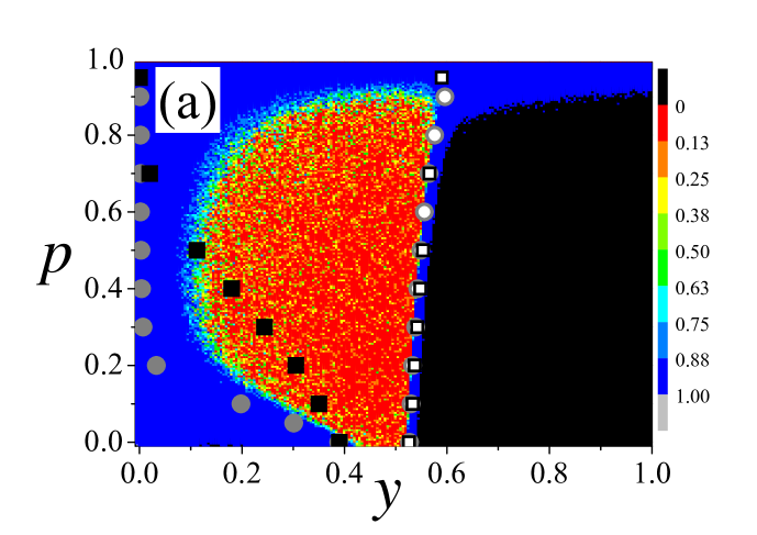
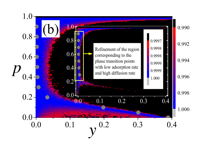
Figure 1: (a) Coefficient of determination $r$ as function of $y$ and $p$ using the algorithm I and the TDMC simulations. The filled and empty black squares correspond, respectively, to the continuous and discontinuous phase transitions predicted in Ref. [19]. In this same figure, we also show the results of the SSMC simulations for the algorithm I: The filled and empty filled gray circles correspond, respectively, to the continuous and discontinuous transition points. (b) Refinement of region with low adsorption rate and high diffusion rate.

As can be seen, there are two regions that deserve more attention, i.e., regions in which the points $(y,p)$ possess coefficient of determination close to 1 (the blue regions in the figure). The first one is around the continuous phase transition point of the original ZGB model, $y\cong 0.3875$, with $p=0$. The second one is close to $y\cong 0.525$, which is the discontinuous phase transition point of the original ZGB model, with $p$ ranging from 0 to 1. We can observe two very different behaviors: the discontinuous phase transition of the model is not influenced by the diffusion of the adsorbed atoms/molecules but the continuous one is strongly affected.

The filled and empty black squares show, respectively, the continuous and discontinuous points estimated in Ref. [19] by using standard SSMC simulations. Even though the protocols and algorithms are different, one can be seen that the discontinuous phase transition points perfectly agree with our vertical discontinuous phase transition line (blue line) obtained through TDMC simulations. However, the continuous phase transition points obtained in Ref. [19] present a huge difference from our estimates since they cross the red/orange region with small coefficient of determination, $r\approx 0-0.25$. However, it is important to mention that the algorithm I does not correspond to the method employed in Ref. [19] which is defined by the protocol II (DIF-II) and algorithm III that is considered in the Subsec. 4.3.

In this same figure, we also show the estimates obtained through SSMC simulations (see Fig. 2) represented by filled and empty gray circles, which refer to some continuous and discontinuous phase transitions points, respectively, as can be seen in Table 2.

	Discontinuous phase transition					Continuous phase transition
${\small p}$	Algorithm					Algorithm
	I	II	III	IV	Ref. [19]	I	II	III	IV	Ref. [19]
0.00	0.527(2)	0.527(1)	0.527(1)	0.527(2)	0.526(1)	0.389(1)	0.389(1)	0.389(1)	0.389(2)	0.390(1)
0.10	0.530(2)	0.525(2)	0.532(1)	0.530(2)	0.533(1)	0.301(1)	0.219(1)	0.349(1)	0.352(2)	0.350(1)
0.20	0.533(2)	0.522(2)	0.537(2)	0.531(3)	0.537(1)	0.198(2)	0.112(1)	0.302(1)	0.321(2)	0.305(1)
0.30	0.539(3)	0.521(2)	0.542(2)	0.532(3)	0.542(1)	0.033(2)	0.059(2)	0.249(2)	0.291(3)	0.244(1)
0.40	0.543(3)	0.519(2)	0.547(2)	0.533(3)	0.548(1)	0.007(3)	0.034(2)	0.185(2)	0.263(3)	0.180(1)
0.50	0.549(3)	0.517(3)	0.552(2)	0.533(3)	0.553(2)	0.004(3)	0.025(3)	0.119(2)	0.236(3)	0.112(2)
0.60	0.556(4)	0.514(3)	0.558(3)	0.534(4)	-	0.003(3)	0.022(4)	0.056(3)	0.204(4)	-
0.70	0.565(4)	0.512(4)	0.567(3)	0.534(4)	0.566(5)	0.002(4)	0.017(4)	0.018(3)	0.185(4)	$\approx$ 0.02
0.80	0.576(5)	0.511(4)	0.578(5)	0.534(5)	-	0.002(5)	0.015(5)	0.006(4)	0.164(6)	-
0.90	0.596(6)	0.508(5)	0.595(7)	0.534(6)	-	0.001(7)	0.011(6)	0.003(6)	0.142(8)	-
0.95	-	-	-	-	0.59(1)	-	-	-	-	$\approx$ 0

Table 2: Phase transition points for the four algorithms obtained through SSMC simulations.

As can be seen, the discontinuous phase transition line is very robust since all three results, obtained with different techniques and different algorithms, are in absolut agreement with each other.

Figure 1 (b) shows a refinement of the coefficient of determination for continuous phase transition region. This refinement process is a straightforward procedure: we consider only values of $r$ ranging from 0.990 to 1 to construct the color map. In this case, one can observe an interesting narrowing of the blue regions which remain containing the filled gray circles. A further refinement of $r$ ($0.9997\leq r\leq 1$) is showed in the inset plot of Fig. 1 (b) and confirm that our results obtained via TDMC simulations are in complete agreement with those ones obtained through SSMC simulations.

Figure 2 shows the density of empty sites $(V)$, $CO_{2}$ and $CO$ molecules, and $O$ atoms as function of $y$, for different values of $p$. We can clearly observe the continuous and discontinuous phase transition points when $y$ and $p$ vary. These points are, respectively, the filled and empty gray circles already presented in Fig. 1.

.

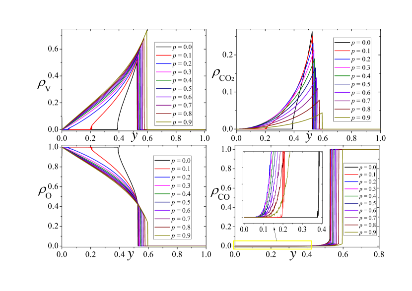
Figure 2: Density of empty sites $V$, $CO_{2}$ molecules, $O$ atoms, and $CO$ molecules as function of $y$, for different values of $p$, obtained through SSMC simulations for the algorithm I. We can observe the continuous and discontinuous phase transitions in all of these curves. In the last plot, for density of $CO$, the inset plot shows a zoom of the continuous phase transition region $0<y<0.4$

Just for completing the study of the algorithm I, we wonder about the existence of correlation between the negativity/positivity of the exponent $\lambda$ and the region of maximum coefficient of determination. It is important to mention that this is only an empirical analysis. In Fig. 3, we show the color map of the exponent $\lambda$ (Eq. 7) as function of $y$ and $p$ for the region of the continuous phase transition along with our results obtained by SSMC simulations. The figure suggests that $\lambda$ lies between -1.10 and -0.7.

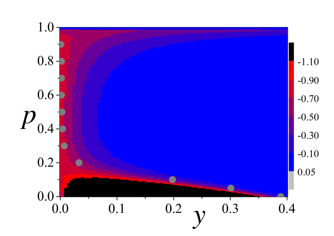
Figure 3: Exponent $\lambda$ as function of $y$ and $p$ obtained through TDMC simulations for the algorithm I in the region of the continuous phase transition.

As shown above, in our study, we are able to localize both continuous and discontinuous phase transitions of the model by means of TDMC simulations along with the coefficient of determination approach. The combination of this two techniques has been proven to be very efficient in determining the second order phase transition points of several models with and without defined Hamiltonians, and with absorbing phases. At the very beginning, it was not expected that TDMC simulations were able to estimate first order phase transitions. However, it has been shown that it is possible to determine, at least, weak first order phase transition points [46] through this technique. Recently, some works have shown the efficiency of this combination in determination the weak first order phase transitions of systems with and without defined Hamiltonians [34, 37].

From now on, we mantain the convention adopted until now for the figures, i.e., gray circles refer to the results obtained in our SSMC simulations and black squares denote the results taken from literature, more precisely from the Ref. [19]. The continuous phase transition points are represented by filled circles or squares and the discontinuous ones are represented by empty circles or squares.

Now, we consider the other order parameter of the model, the density of $CO$ molecules ($\rho_{CO}$), just for looking into the behavior of the exponent $\lambda$, i.e., its sign and absolute value, for the region of the discontinuous phase transition. The reason for choosing this order parameter in this analysis is that, as happen to the density of vacant sites $\rho_{V}$, its time evolution does not present huge fluctuations in this region. In addition, the region of interest is narrower and better defined for $\rho_{CO}$. Figure 4 (a)) shows the color map of the exponent $\lambda$ as function of $y$ and $p$ when considering $\rho_{CO}$ as the order parameter, and also the refinement $\lambda\leq 0$. We can observe from this plot that negative exponents are discarded for the discontinuous phase transition points.

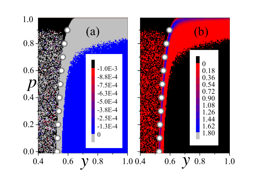
Figure 4: (a) Exponents $\lambda$ as function of $y$ and $p$ obtained through TDMC simulations for the algorithm I in the region of the discontinuous phase transition points for $\rho_{CO}$ with the refinement $\lambda\leq 0$. (b) The same plot with the refinement $\lambda>0$.

Figure 4 (b) refines the region for $\lambda>0$. We can observe that when the larger the magnitude of the exponent, the better is the agreement with the discontinuous phase transition points. So, the exponent can be an interesting indicator to locate continuous and discontinuous phase transition points in surface reaction models. However, further studies must be performed in this direction. From now on, we focus only on the coefficient of determination. In the next subsection we present our results for the protocol DIF-I and algorithm II.

4.2 Algorithm II: Protocol DIF–I with “OR” adsorption process

In this subsection, we perform simulations following the algorithm II in which both diffusion and adsorption processes can occur in the same trial, i.e., the diffusion does not exclude the possibility of the adsorption. As can be seen in Fig. 5, the analysis of the results are similar to those presented above, i.e., the TDMC simulations are also supported by the SSMC simulations. We also show the estimates obtained in Ref. [19] which are presented in Table LABEL:Table:ssmc.

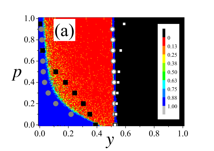
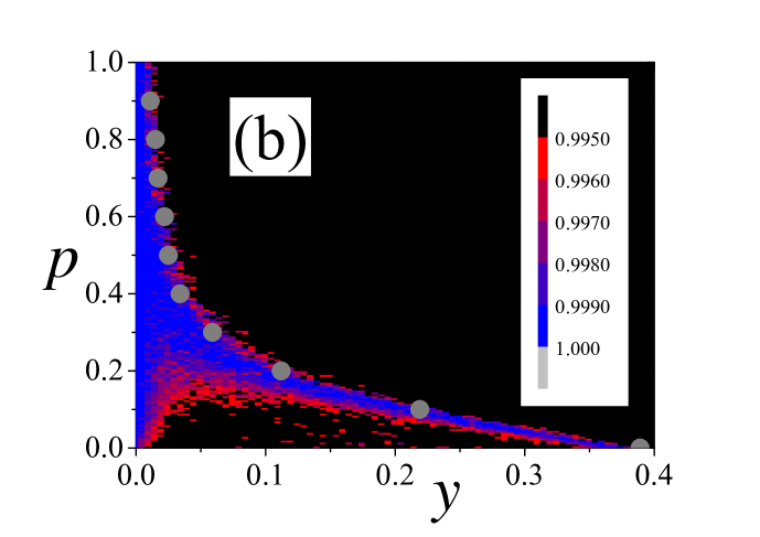
Figure 5: (a) Coefficient of determination $r$ as function of $y$ and $p$ obtained with the protocol DIF-I and the algorithm II through TDMC simulations, as well as the results of SSMC simulations. The filled and empty black squares correspond, respectively, to the continuous and discontinuous phase transitions predicted in Ref. [19], and the filled and empty filled gray circles correspond, respectively, to the continuous and discontinuous transition points, both obtained via SSMC simulations. (b) Refinement of the region of continuous phase transition points.

The plots (a) and (b) of this figure correspond to the Fig. 1 (a) and (b), respectively, and their format are similar. In fact, it is important to notice that the discontinuous phase transition points of Fig. 1 remain practically the same as shown in Fig. 5 (a). In this same plot, we show that the results of our SSMC simulations is in complete agreement with those obtained via TDMC simulations. Figure 5 (b) presents a refinement of the coefficient of determination for the region of the continuous phase transition. As shown in Fig. 1, this refinement narrows the blue prolongation making clearer that the coefficient of determination perfectly matches the gray points obtained by SSMC simulations. These gray points are obtained exactly as those presented in Fig. 2 for the algorithm I, and therefore, we find it unnecessary to show their figures here.

In addition, we also present the points obtained in Ref. [19]. Those points do not match any of the regions of phase transition, differently from what we find for algorithm I, in which its discontinuous phase transition points are in complete agreement with ours. This difference is expected since we are not dealing with the same algorithm. However, this emphasizes an important point: the discontinuous line is more sensitive to how the diffusion is combined with adsorption than the way the diffusion is considered in the model.

4.3 Algorithms III and IV, and the effects of $N_{run}$ and $L$ on the coefficient of determination

Now, we combine the protocol DIF-II with the prescriptions I and II, with we call algorithms III and IV, to study, as above, the influence of the diffusion of the atoms/molecules on the lattice. Thus, following the last two subsections, we obtain the coefficient of determination for the algorithms III and IV, whose results are shown in Fig. 6. The results obtained via SSMC simulations are also present in this figure and in Table LABEL:Table:ssmc.

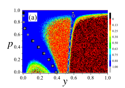
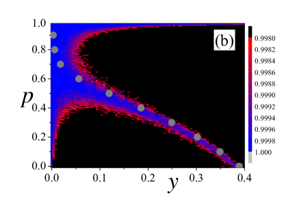
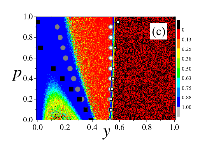
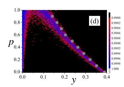
Figure 6: Coefficient of determination $r$ as function of $y$ and $p$. The algorithm III is represented by the plots (a) and (b), and the results for the algorithm IV is shown in the plots (c) and (d). Following the same procedure as in the previous figures, (a) and (c) are the complete diagrams while (b) and (d) are the refinements of the regions corresponding to the continuous phase transition.

Figures 6 (a) and (b) represent the algorithm III and correspond, respectively, to the complete diagram and the region of continuous phase transition after the refinement procedure. From Fig. 6 (a), it is clear that the algorithm III must be the corresponding model used in Ref. [19] since our points obtained via SSMC simulations (grey circles) are in complete agreement with the points extracted from that paper (black squares) in both regions. In Fig. 6 (c) and (d), we show our results based on the algorithm IV. In that case, we can observe that our estimates for the region of continuous phase transition is completely different from those presented in Ref. [19]. On the other hand, there is only a slightly difference between them in the region of the discontinuous phase transition.

So, with the results of the four algorithms in hand, we can consider some important points. First, the choice of XOR or OR to combine the diffusion and adsorption processes seems to be more important to the region of continuous phase transition that to the region of discontinuous one, since we have a complete agreement between algorithms I and III which share the same prescription (diffusion process XOR adsorption process) but possess different protocols for the diffusion (DIF-I and DIF-II, respectively). In addition, we have a certain similarity between the algorithms II and IV which also share the same prescription (diffusion process OR adsorption process) with different protocols, DIF-I and DIF-II, respectively. On the other hand, the choice of the diffusion protocol leads to more similarity in the region of continuous phase transition as can be observed between the algorithms I and II and also between the algorithms III and IV.

For high diffusion rates, $p\rightarrow 1$, the rule XOR (prescription I) completely suppress the possibility of the adsorption of atoms/molecules on the lattice, generating false positive regions that makes it difficult to locate the continuous phase transition points. So, only with the high resolution obtained through the refinement process, we are able to locate such points independently of what diffusion process is used.

Finally, important questions can be raised about the parameters considered in our TDMC simulations such as the linear size of the square lattice, $L=80$, and the number of runs, $N_{run}=5000$. From these two parameters, the lattice size seems to be the most relevant one since in Ref. [19] the authors consider lattices of linear size $L=500$ in the study of the continuous phase transitions of the model. To supress any doubts, we prepare as an example, a simple plot in which we fix the adsorption rate in $y=0.112$ and calculate the coefficient of determination $r$ as function of $p$ for the algorithm III with several values of $L$ and $N_{run}$. According to the Ref. [19] is expected that the maximun value of $r$, for sufficienly large lattices, should occur for $p\approx 0.5$. Figure 7 shows the curve $r$ $\times p$ for five different lattice sizes and three different number of runs.

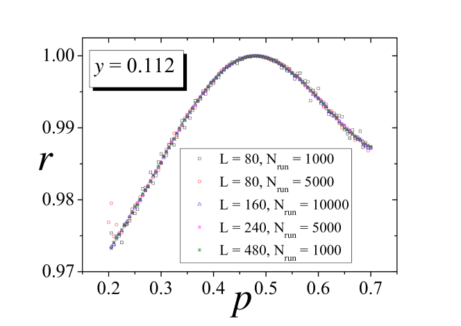
Figure 7: Effects of $L$ and $N_{run}$ on the coefficient of determination $r$. The optimization curve $r\times p$ shows that there is no noticeable difference among the five curves obtained for diferent values of $L$ and of $N_{run}$.

As can be observed, there is no significant difference among the curves, mainly in the region of highest value of $r$. This example, along with other simulations performed initially, shows that our choice of the parameters $L=80$ and $N_{run}=5000$ is appropriate and garantee that our results are reliable and robust.

5 Conclusions

In this work, we studied a modified version of the Ziff-Gulari-Barshad (ZGB) model to include the spatial diffusion of the $O$ atoms and $CO$ molecules adsorbed on the surface through four different algorithms. By using an alternative method that optimizes the coefficient of determination, we were able to localize the regions of continuous and discontinuous phase transitions of the model. Our results showed that, for all algorithms, the critical behaviour is strongly changed by introducing the diffusion of the atoms/molecules. On the contrary, the discontinuous phase transition in much less sensitive to the diffusion even when the diffusion rate is high. Our results were obtained through time-dependent Monte Carlo (TDMC) simulations based on the optimization of the coefficient of determination which took into account the time evolution of the two order parameters of the model: the densities of vacant sites, $\rho_{V}$, and of $CO$ molecules, $\rho_{CO}$. All the results were corroborated by steady-state Monte Carlo (SSMC) simulations.

The four algorithms were constructed in such a way that the diffusion and adsorption processes are combined in two ways. In addition, there are also two ways to implement the diffusion. We presented these algorithms as algorithm I, II, III, and IV, and we showed that only the algorithm III corresponds to the results found in the literature. In that case, only one process is allowed in each trial, the diffusion process or the adsorption process, and the diffusion of an atom/molecule changes with the number of the empty sites in its neighbourhood.

In summary, this work classified the problem of diffusion in surface reaction models (more precisely in the ZGB model) and showed that the problem can be solved via TDMC simulations based on the optimization of a simple statistical concept, the coefficient of determination. As show in the figures, the TDMC simulations were in line with our SSMC simulations which confirmed the efficiency of the coefficient of determination in estimating the phase transitions of the model.

References

- [1] R.M. Ziff, E. Gulari, and Y. Barshad, Phys. Rev. Lett. 56, 2553 (1986).
- [2] P. Meakin and D.J. Scalapino, J. Chem. Phys. 87, 731 (1987).
- [3] R. Dickman, Phys. Rev. A 34, 4246 (1986).
- [4] P. Fischer and U.M. Titulaer, Surf. Sci. 221, 409 (1989).
- [5] G.C. Bond, Catalysis: Principles and Applications (Clarendon, Oxford, 1987).
- [6] V.P.Z. Zhdanov and B. Kazemo, Surf. Sci. Rep. 20, 113 (1994).
- [7] J. Marro and R. Dickman, Nonequilibrium Phase Transitions in Lattice Models (Cambridge University Press, Cambridge, U.K., 1999).
- [8] A. Golchet and J.M. White, J. Catal. 53, 266 (1978).
- [9] T. Matsushima, H. Hashimoto, and I. Toyoshima, J. Catal. 58, 303 (1979)
- [10] M. Ehsasi, M. Matloch, J.H. Block, K. Christmann, F.S. Rys, and W. Hirschwald, J. Chem. Phys. 91, 4949 (1989).
- [11] K. Christmann, Introduction to Surface Physical Chemistry (Steinkopff Verlag, Darmstadt, 1991), pp. 1274.
- [12] J.H. Block, M. Ehsasi, and V. Gorodetskii, Prog. Surf. Sci. 42, 143 (1993).
- [13] H.K. Janssen, B. Schaub, and B. Schmittmann, Z. Phys. B: Condens. Matter 73, 539 (1989).
- [14] G. Grinstein, Z.-W. Lai, and D.A. Browne, Phys. Rev. A 40, 4820 (1989).
- [15] M. Dumont, P. Dufour, B. Sente, and R. Dagonnier, J. Catal. 122, 95 (1990).
- [16] E.V. Albano, Appl. Phys. A 54, 2159 (1992).
- [17] T. Tomé and R. Dickman, Phys. Rev. E 47, 948 (1993).
- [18] H.P. Kaukonen and R.M. Nieminen, J. Chem. Phys. 91, 4380 (1989).
- [19] I. Jensen and H. Fogedby, Phys. Rev. A 42, 1969 (1990).
- [20] G.M. Buendia , E. Machado, and P.A. Rikvold, J. Chem. Phys. 131, 184704 (2009).
- [21] B.C.S. Grandi and W. Figueiredo, Phys. Rev. E 65, 036135 (2002).
- [22] G.L. Hoenicke and W. Figueiredo, Phys. Rev. E 62, 6216 (2000).
- [23] G. M. Buendía and P.A. Rikvold, Phys. Rev. E 85, 031143 (2012).
- [24] G. M. Buendía and P.A. Rikvold, Phys. Rev. E 88, 012132 (2013).
- [25] G.M. Buendía, P.A. Rikvold, Phys. A. 424, 217 (2015).
- [26] G.L. Hoenicke, M.F. de Andrade, and W. Figueiredo, J. Chem. Phys. 141, 074709 (2014).
- [27] J. Satulovsky and E.V. Albano, J. Chem. Phys. 97, 9440 (1992).
- [28] E.V. Albano, Surf. Sci. 235, 351 (1990).
- [29] B.J. Brosilow, E. Gulari, and R.M. Ziff, J. Chem. Phys. 98, 674 (1993).
- [30] K. S. Trivedi, Probability and Statistics with Realiability, Queuing, and Computer Science and Applications, 2nd ed. (John Wiley and Sons, Chichester, 2002).
- [31] R. da Silva, J.R. Drugowich de Felício, A.S. Martinez, Phys. Rev. E. 85, 066707 (2012).
- [32] R. da Silva, N. Alves Jr., J.R. Drugowich de Felicio, Phys. Rev. E 87, 012131 (2013).
- [33] R. da Silva, H.A. Fernandes, J.R. Drugowich de Felício, W. Figueiredo, Comput. Phys. Commun. 184, 2371 (2013).
- [34] R. da Silva, H.A. Fernandes, J.R. Drugowich de Felício, Phys. Rev. E 90, 042101 (2014).
- [35] H.A. Fernandes, R. da Silva, A. A. Caparica, J. R. Drugowich de Felicio, Phys. Rev. E 95, 042105 (2017)
- [36] R. da Silva, H.A. Fernandes, J. Stat. Mech. P06011 (2015)
- [37] H.A. Fernandes, R. da Silva, E.D. Santos, P.F. Gomes, and E. Arashiro, Phys. Rev. E 94, 022129 (2016).
- [38] W. Evans and M. S. Miesch, Phys. Rev. Lett. 66, 833 (1991).
- [39] E.V. Albano, Chem. Rev. 3, 389 (1996).
- [40] C.A. Voigt, R.M. Ziff, Phys. Rev. E 56 R6241 (1997)
- [41] R.M. Ziff and B.J. Brosilow, Phys. Rev. A, 46 4630 (1992).
- [42] R. da Silva, N.A. Alves and J.R. Drugowich de Felício, Phys. Lett. A 298, 325 (2002).
- [43] H.A. Fernandes, Roberto da Silva, and J.R. Drugowich de Felicio, J. Stat. Mech.: Theor. Exp., P10002 (2006).
- [44] R. da Silva, R. Dickman, and J.R. Drugowich de Felício, Phys. Rev. E 70, 067701 (2004)
- [45] P. Grassberger and Y. Zhang, Physica A 224, 169 (1996)
- [46] L. Schulke and B. Zheng, Phys. Rev. E 62, 7482-7485 (2000)
- [47] E. Albano, Physics Letters A 288, 73–78 (2001)