Propagation of Electron-Acoustic Waves in a Plasma with Suprathermal Electrons

Ashkbiz Danehkar

A thesis submitted to the Queen’s University Belfast for the Degree of Master of Science in Plasma Physics

Centre for Plasma PhysicsDepartment of Physics & AstronomyQueen’s University BelfastBelfast BT7 1NN, United Kingdom December 2009

Electron-acoustic waves occur in space and laboratory plasmas where two distinct electron populations exist, namely cool and hot electrons. The observations revealed that the hot electron distribution often has a long-tailed suprathermal (non-Maxwellian) form. The aim of the present study is to investigate how various plasma parameters modify the electron-acoustic structures. We have studied the electron-acoustic waves in a collisionless and unmagnetized plasma consisting of cool inertial electrons, hot suprathermal electrons, and mobile ions. First, we started with a cold one-fluid model, and we extended it to a warm model, including the electron thermal pressure. Finally, the ion inertia was included in a two-fluid model. The linear dispersion relations for electron-acoustic waves depicted a strong dependence of the charge screening mechanism on excess suprathermality. A nonlinear (Sagdeev) pseudopotential technique was employed to investigate the existence of electron-acoustic solitary waves, and to determine how their characteristics depend on various plasma parameters. The results indicate that the thermal pressure deeply affects the electron-acoustic solitary waves. Only negative polarity waves were found to exist in the one-fluid model, which become narrower as deviation from the Maxwellian increases, while the wave amplitude at fixed soliton speed increases. However, for a constant value of the true Mach number, the amplitude decreases for increasing suprathermality. It is also found that the ion inertia has a trivial role in the supersonic domain, but it is important to support positive polarity waves in the subsonic domain.

I confirm the following:

(i) the dissertation is not one for which a degree has been or will be conferred by any other university or institution;

(ii) the dissertation is not one for which a degree has already been conferred by this university;

(iii) that this work submitted for assessment is my own and expressed in my own words. Any use made within it of works of other authors in any form (e.g. ideas, figures, text, tables) are properly acknowledged at their point of use. A list of the references employed is included;

(iv) the composition of the dissertation is my own work.

Ashkbiz Danehkar
December 2009

The author would like to thank Dr. Ioannis Kourakis, Lecturer at the Queen’s University Belfast for his supervision and guidance throughout the project, Dr. Nareshpal Singh Saini, Post-doctoral Researcher at the Queen’s University Belfast, Prof. Manfred A. Hellberg, Emeritus Professor at the University of KwaZulu-Natal, for their collaborations, providing consultations and valuable comments. This research has been supported by a grant from the Department for Employment and Learning (DEL) in Northern Ireland (A.D.), and a contract from the Engineering and Physical Sciences Research Council (UK EPSRC) (N.S.S. & I.K.). The research is also supported in part by the National Research Foundation of South Africa (NRF) (M.A.H.). Any opinion, findings, and conclusions or recommendations expressed in this material are those of the authors and therefore the NRF does not accept any liability in regard thereto.

1 Introduction

The electron-acoustic waves (EAWs) usually occur in a plasma, where inertial cool electrons oscillates against inertialess hot electrons. EAWs may exist in plasmas with two electrons population referred to as cool  (hot) electrons with respective temperatures $T_{c}$ ($T_{h}$). These are typically high-frequency (in comparison with the ion plasma frequency) electrostatic waves propagating with the phase velocity intermediate between hot and cool electron thermal velocities. At such high frequency, the positive ions behave like uniformly distributed charge background providing charge neutrality, but they have no essential role in the dynamics (of supersonic negative solitary waves; see 4.3). The phase velocity of the EAWs is much larger than the cool electron thermal velocity and much smaller than the hot electron thermal velocity. The cool electrons provide the inertial effects needed to maintain the EAWs, while the restoring force comes from the pressure of the hot electrons.

As the temperature rises in a collisionless plasma, the phase velocity of waves become comparable with the electron thermal velocities. In a situation depends on the electron thermal velocity (faster/slower than the phase velocity), a direct interaction between electrons and waves produces the Landau damping (wave heating) or inverse Landau damping (instabilities) through the Vlasov kinetic theory (no need of a collision term). When the phase velocity goes near the thermal velocity for a short wavelength, the Landau damping become very strong, i.e., the wave cannot propagate in the plasma. This means that the propagation of EAWs is possible within a restricted range of parameters. It has been proven that the EAWs are not damped at the temperature ratio $T_{c}/T_{h}\lesssim 0.1$ [1, 2] and the cool electrons at a significant fraction of the total electron density: $0.2\lesssim n_{c}/(n_{c}+n_{h})\lesssim 0.8$ [2, 3], as illustrated in Fig. 1.1. The wave number $k$ of the weakly damped EAW is between roughly $0.2\lambda_{Dc}^{-1}$ and $0.6\lambda_{Dc}^{-1}$ (where $\lambda_{Dc}$ is the cool electron Debye length). The temperature and the number density of the cool and hot electrons modify the stable range of the wave number (see e.g. Figs. 1–3 in [2]; or Fig. 2.1(b) and Fig. 3.1).

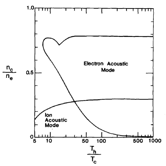
Figure 1.1: The parameter space of the cool-to-total electron density ratio versus the hot-to-cool temperature ratio for weakly damped electron-acoustic waves and ion-acoustic waves [2].

The EAWs often occur in laboratory experiments [4, 5, 6] and space plasmas e.g. the Earth’s bow shock [7, 8, 9] and the auroral magnetosphere [3, 10]. Another example is the Broadband Electrostatic Noise (BEN), a common wave activity in the plasma sheet boundary layer (PSBL) region, which has been observed by the satellites missions [11, 12, 13, 14]. The BEN emissions forming as EAWs, which include a series of isolated bipolar pulses, have the frequency range from $\sim 10$ Hz upto the local electron plasma frequency ($\sim 10$ kHz) [11]. This suggests that the emissions are related to electron dynamics rather than ions [11, 14].

In two electron temperature plasmas, two electrons population are often characterized by a thermal Maxwellian distribution [15, 16, 17, 18]. However, some space and laboratory plasmas have such a suprathermal electron population, whose behaviors are extremely different from a Maxwellian distribution. Electrons obey an inverse power law distribution at a velocity much higher than the electron thermal velocity. We describe this suprathermal population by a generalized Lorentzian or $\kappa$-distributions [19, 20, 21].

The common form of the isotropic (three-dimensional) generalized Lorentzian or $\kappa$-distribution function is given by [20, 21, 22]

$$f_{\kappa}(v)=n_{0}(\pi\kappa\theta^{2})^{-3/2}\frac{\Gamma(\kappa+1)}{\Gamma(\kappa-\frac{1}{2})}\left(1+\frac{v^{2}}{\kappa\theta^{2}}\right)^{-\kappa-1}.$$ (1.1)

where $n_{0}$ is an equilibrium number density of the electrons, $v$ the species velocity, $\theta$ is a generalized thermal velocity related to the actual thermal velocity of the electrons $v_{th,e}=(2k_{B}T_{e}/m_{e})^{1/2}$ by $\theta=v_{th,e}\left((\kappa-\tfrac{3}{2})/\kappa\right)^{1/2}$; $k_{B}$ the Boltzmann constant, $m_{e}$ and $T_{e}$ the mass and temperature of the electrons, respectively. We note that $\kappa$ is the spectral index of $\kappa$-distributions with $\kappa>\frac{3}{2}$. For $\kappa\rightarrow\infty$, we have a Maxwellian, while low values of $\kappa$ are associated with significant numbers of suprathermal particles. The gamma function $\Gamma$ arises from the normalization of $f_{\kappa}(v)$, i.e. $\int f_{\kappa}(v)d^{3}v=n_{0}$.

The $\kappa$-distribution has been firstly applied to model velocity distribution of particles observed in space plasmas, often in the range $2<\kappa<6$ [23]. The $\kappa$-distribution function can describe laboratory experiments and space plasmas more effectively than a Maxwellian function [8, 19, 24, 25, 26, 27]. For example, measurements of plasma sheet electron and ion distributions can be treated by $\kappa_{i}=4.7$ and $\kappa_{e}=$ $5.5$ [24] (here, $e$ denotes electrons and $i$ ions), observations in the earth’s foreshock satisfying $3<\kappa_{e}<6$ [8], and coronal electrons in solar wind model with $2<\kappa_{e}<6$ [27].

Studies of linear and nonlinear EAWs in plasmas with nonthermal electrons have received a great deal of interest in recent years [25, 28, 29, 30, 31, 32, 33, 34, 35, 22]. The linear analysis of EAWs, which provided a dispersion relation, was firstly described in an unmagnetized homogenous plasma [36]. It exhibited a heavily damped acoustic-like solution in addition to the Langmuir waves and ion-acoustic waves (IAWs) [36]. The linear properties with suprathermal particles provided dispersion functions [25, 28, 29, 30]. It shows the effect of suprathermal electrons on propagation of EAWs, which increase the Landau damping of the wave at small wave numbers (acoustic regime) [29], and the dependence of the Landau damping on the fraction of suprathermal electrons [30]. Large values of $\kappa$ (quasi-Maxwellian) produce weaker Landau damping in the acoustic regime, while Landau damping increases by hot electrons for small values of $\kappa$ [29].

The nonlinear analysis of the EAWs in a one-dimensional unmagnetized plasma composed of cold and hot electrons has been shown the existence of negative potential soliton [31], while additional electron beam component leads to a positive potential soliton [32]. The nonlinear aspects of EAWs in an unmagnetized plasma consisting of nonthermal electrons, fluid cold electrons, and ions provided negative potential solitary structures [33].

1.1 Thesis Outline

We used a strategic workplan and some steps for this work. The analytical basis for the 3 models is presented in the Appendix A. We discuss the outcomes of each model for the linear dispersion relation and the existence conditions of stationary profile solitary structures. The organization of the thesis is as follows:

In Chapter 2, we have performed a preliminary work on a one-fluid cold ($T_{c}=0$) model consisting of cold electron and background of hot suprathermal electrons and stationary ions, i.e., only cold electrons treated as a fluid. We study the linear and nonlinear effects of the hot suprathermal electrons on electron-acoustic (EA) waves, namely the weakly damped region and the propagation velocity range.

In Chapter 3, we extended it to the one-fluid warm electrons model, which includes the pressure of the cool ($T_{c}\neq 0$) electrons. Comparing with the one-fluid cold model, we investigate the effect of the “cool-electron”temperature. We distinguish two regimes for the propagation velocity, namely subsonic (slow) and supersonic (fast) scales. We have treated the cool electrons to be supersonic (i.e. having a propagation speed above the electron thermal speed), and have found that only negative solitary structures can exist on this (fast) scale.

In Chapter 4, we assume that ions are no longer stationary, i.e., treated as a fluid to make a two-fluid model consisting of cool electron-fluid, ion-fluid, and hot background of suprathermal electrons. We see that the ion-fluid does not influence much the fast negative solitons, while producing novel positive solitary structures on the slow scale. We also investigate the nonlinear effects of the hot suprathermal electrons on the positive acoustic solitary waves, i.e., the electric potential pulse and the propagation velocity range.

Finally, our main findings and conclusions are summarized in Chapter 5.

2 Cold Electron Fluid with Suprathermal Electrons

In this chapter, we study the EAWs in an unmagnetized plasma composed of cold ($T_{c}=0$) electron fluid, hot suprathermal $\kappa$-distributed electrons, and uniformly distributed ions. We present the basic set of equations of the model in §2.1. In §2.2, we derive the dispersion relation for the linear dynamics of EAWs. In §2.3, we obtain the nonlinear structures of the electrostatic solitary waves and describe the soliton existence domain.

2.1 Basic Equations

We consider a plasma with three components, namely cold electron-fluid, inertialess hot electron component with a suprathermal (non-Maxwellian) electron velocity distribution, and uniform ion background. The cold electron-fluid governing the linear and nonlinear dynamics of electron-acoustic waves (EAWs) feels the effect of the hot suprathermal electrons. To study the linear and nonlinear results, we obtain the normalized fluid-moment equations and the Poisson’s equation through some appropriate scales.

The number density of cold electrons is governed by the continuity equation

$$\frac{\partial n_{c}}{\partial t}+\frac{\partial(n_{c}u_{c})}{\partial x}=0.$$ (2.1)

The cold electrons obey the momentum equation

$$\frac{\partial u_{c}}{\partial t}+u_{c}\frac{\partial u_{c}}{\partial x}=\frac{e}{m_{e}}\frac{\partial\phi}{\partial x}.$$ (2.2)

The densities of suprathermal hot electron, fluid cold electrons and uniform ions are related to the electrostatic potential by the Poisson’s equation:

$$\frac{\partial^{2}\phi}{\partial x^{2}}=-\frac{e}{\varepsilon_{0}}\left(n_{i}-n_{c}-n_{h}\right),$$ (2.3)

where $\varepsilon_{0}$ is the permittivity constant.

The uniform ions mean that $n_{i}=n_{i,0}=$ const, where $n_{i0}$ is the undisturbed ion density. We need an expression for the number density of the hot electron, $n_{h}$, which takes into account the suprathermal distribution (1.1). Integrating Eq. (1.1) over velocity space, we obtain the number density of the suprathermal hot electrons given by [21]

$$n_{h}(\phi)=n_{h,0}\left(1-\frac{e\phi}{k_{B}T_{h}(\kappa-\tfrac{3}{2})}\right)^{-\kappa+1/2},$$ (2.4)

where $n_{h,0}$ is the density of hot electrons in the undisturbed plasma, $T_{h}$ the temperature of hot electron, $\phi$ the electrostatic wave potential, $e$ the elementary charge, and $\kappa$ a spectral index which measures deviation from thermal equilibrium.

At equilibrium, the plasma is assumed to be quasi-neutral

$$n_{c,0}+n_{h,0}=Zn_{i,0}.$$ (2.5)

In addition, we define the equilibrium density ratios of the ions to the cold electrons and of the hot electrons to the cold electrons, respectively:

$$\begin{array}[c]{cc}\alpha\equiv\dfrac{n_{i,0}}{n_{c,0}},&\text{ }\beta\equiv\dfrac{n_{h,0}}{n_{c,0}}.\end{array}$$ (2.6)

We assume that $Z=1$ everywhere. Using above definition, Eq. (2.5) take the form as $\alpha=1+\beta$. According to [3], the propagation of the EAWs remain undamped in the range $0.2\lesssim n_{c,0}/(n_{c,0}+n_{h,0})\lesssim 0.8$. Therefore, the following condition is satisfied: $0.25<\beta<4$. This is a range for the existence of electron-acoustic solitary waves.

If we scale densities by $n_{c,0}$, we can write Eq. (2.4) in dimensionless form as

$$n_{h}(\phi)=\beta\left(1-\frac{\phi}{\kappa-\tfrac{3}{2}}\right)^{-\kappa+1/2}.$$ (2.7)

In the limit $\kappa\rightarrow\infty$, Eq. (2.7) is reduced to $n(\phi)=\beta\exp(\phi)$, the Maxwellian distributions for the electrons.

It is convenient to use the nondimensional form of Eqs. (2.1)–(2.3):

$$\frac{\partial n}{\partial t}+\frac{\partial(nu)}{\partial x}=0,$$ (2.8)

$$\frac{\partial u}{\partial t}+u\frac{\partial u}{\partial x}=\frac{\partial\phi}{\partial x},$$ (2.9)

$$\frac{\partial^{2}\phi}{\partial x^{2}}=-(1+\beta)+n+\beta\left(1-\frac{\phi}{\kappa-\tfrac{3}{2}}\right)^{-\kappa+1/2},$$ (2.10)

which is done by choosing the variables as

$$\begin{array}[c]{ccccc}\dfrac{n_{c}}{n_{c,0}}\rightarrow n,\text{ }&\dfrac{\phi}{k_{B}T_{h}/e}\rightarrow\phi,\text{ }&\dfrac{u_{c}}{c_{h,s}}\rightarrow u,\text{ }&t\omega_{pc}\rightarrow t,\text{ }&\dfrac{x}{\lambda_{0}}\rightarrow x,\end{array}$$ (2.11)

where the sound speed of hot electrons is defined by $c_{h,s}=(k_{B}T_{h}/m_{e})^{1/2}$, the plasma frequency of cold electrons $\omega_{pc}=(n_{c,0}e^{2}/\varepsilon_{0}m_{e})^{1/2}$, and a characteristic length scale $\lambda_{0}=(\varepsilon_{0}k_{B}T_{h}/n_{c,0}e^{2})^{1/2}$.

2.2 Linear Dispersion Relation

In this section, we use linear analysis to derive the dispersion relation for the linear dynamics of EAWs. The linear dispersion relation exhibits that the frequency of the EAWs are less than the cold electron plasma frequency and in the long-wavelength mode the EAWs behave like an ion-acoustic wave.

Let $S$ be any of the system variables $n$, $u$, and $\phi$, describing the system’s state at a given position $x$ and instant $t$. We shall consider small deviations from the equilibrium state $S^{(0)}$, explicitly $n^{(0)}=1$, $u^{(0)}=0$ and $\phi^{(0)}=0$, by taking

$$S=S^{(0)}+S_{1}^{(1)}e^{i(kx-\omega t)}.$$ (2.12)

Accordingly, the derivatives of the first order amplitudes are treated as

$$\begin{array}[c]{cc}\dfrac{\partial S_{1}^{(1)}}{\partial t}=-i\omega S_{1}^{(1)},\text{ }&\dfrac{\partial S_{1}^{(1)}}{\partial x}=ikS_{1}^{(1)}.\end{array}$$ (2.13)

Eqs. (2.8) and (2.9) lead to the following expressions for density and velocity in terms of potential, namely

$$\begin{array}[c]{cc}n_{1}^{(1)}=-\dfrac{k^{2}}{\omega^{2}}\phi_{1}^{(1)},\text{ }&u_{1}^{(1)}=-\dfrac{k}{\omega}\phi_{1}^{(1)}.\end{array}$$ (2.14)

where $\omega$ is the wave frequency and $k$ the wavenumber.

Similarly, the Poisson’s equation (2.10) provides the compatibility condition as

$$-k^{2}\phi_{1}^{(1)}=-\beta-\frac{k^{2}}{\omega^{2}}\phi_{1}^{(1)}+\beta\left(1-\frac{\phi_{1}^{(1)}}{\kappa-\tfrac{3}{2}}\right)^{-\kappa+1/2}.$$ (2.15)

Let us make use of the expansion keeping up to first order:

$$n_{h}(\phi)\approx 1+\frac{\kappa-\frac{1}{2}}{\kappa-\tfrac{3}{2}}\phi.$$ (2.16)

Using above approximate relation, Eq. (2.15) provide the familiar EAWs dispersion relation:

$$\omega_{1}^{2}=\frac{k^{2}}{k^{2}+k_{D}^{2}},$$ (2.17)

where we define $k_{D}$ as

$$k_{D}\equiv\dfrac{1}{\lambda_{D}}\equiv\left(\dfrac{\beta(\kappa-\frac{1}{2})}{\kappa-\tfrac{3}{2}}\right)^{1/2}.$$ (2.18)

Restoring dimensions, we get the standard dispersion relation

$$\omega_{1}^{2}=\omega_{pc}^{2}\frac{k^{2}\lambda_{Dh}^{2}}{k^{2}\lambda_{Dh}^{2}+\left(\dfrac{\kappa-\frac{1}{2}}{\kappa-\tfrac{3}{2}}\right)},$$ (2.19)

where $\lambda_{Dh}$ is the (hot electron) Debye length defined by

$$\lambda_{Dh}=\left(\dfrac{\varepsilon_{0}k_{B}T_{h}}{n_{h,0}e^{2}}\right)^{1/2}=\beta^{-1/2}\lambda_{0}.$$ (2.20)

Eq. (2.19) is recognized as the linear dispersion equation governing our model. This can be represented as curves on a $k$–$\omega$ plane, as dimensionless dispersion relation (2.17) shown in Fig. 2.1. It is important that the EAWs will be deeply damped for the wave number $k$ greater than $0.6k_{D}$. Particularly, the linear EAWs are weakly damped between roughly $0.2k_{D}$ and $0.6k_{D}$ [2, 3]. The stable range of the wave number rises with growing the equilibrium density ratio $\beta=n_{h,0}/n_{c,0}$. The linear EAWs (unlike the well-known Langmuir waves) extends only up to the cold electron plasma frequency. On the other hand, the dispersion relation in the long-wavelength limit (in comparison with $\lambda_{Dh}$) is $\omega\simeq kC_{s}$ where $C_{s}$ is the electron-acoustic sound speed given by

$$C_{s}=\beta^{-1/2}\left(\frac{\kappa-\tfrac{3}{2}}{\kappa-\frac{1}{2}}\right)^{1/2}c_{h,s}.$$ (2.21)

The long-wavelength mode is analogous to an ion-acoustic (IA) mode. Here, the cold electron plays the role of cold ions in the IA mode.

2.2.1 Hot Suprathermal Effect on Linear Waves

As the temperature of the hot electrons is increased, the sound speed within the range of the long-wavelength increases. But, increasing $\beta$or decreasing $\kappa$ reduces the sound speed.

As illustrated in Fig. 2.1, the dispersion curve depends on the parameters $\kappa$ and $\beta$. In the weakly damped region ($0.25<\beta<4$), the slope of the dispersion curve rises with either the increase in $\kappa$ or the decrease in $\beta$. Thus, growing $\beta$ broadens the range of permitted frequencies, within the weakly damped region ($0.2k_{D}<k<0.6k_{D}$).

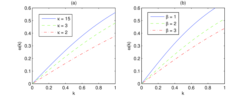
Figure 2.1: Dispersion curves for the linear EAWs. (a) Variation of the dispersion function curve for different values of $\kappa$ and $\beta=2$. Curves from bottom to top: $\kappa=15$ (solid), $3$ (dashed), $2$ (dot-dashed curve). (b) Variation of the dispersion function curve for different values of $\beta$ and $\kappa=4$. Curves from top to bottom: $\beta=1$ (solid), $2$ (dashed), $3$ (dot-dashed curve).

2.3 Nonlinear Electron-Acoustic Solitary Waves

Now, we employ the Sagdeev pseudopotential approach [37] to investigate the nonlinear propagation properties of the cold electrons in a plasma under the effect of the hot suprathermal electrons. In §2.4, we discuss necessary conditions for the generation of solitary structures in the plasma.

We consider solutions of Eqs. (2.8)–(2.10), that are stationary in a frame moving with velocity $M$. We use the Galilean transformation, $\xi=x-Mt$ and $\tau=t$, where $M$ is called the Mach number. This means that all derivatives shall be replaced as follows

$$\begin{array}[c]{cc}\dfrac{\partial}{\partial x}=\dfrac{d}{d\xi},\text{ }&\dfrac{\partial}{\partial t}=-M\dfrac{d}{d\xi}.\end{array}$$ (2.22)

Therefore, Eqs. (2.8)–(2.10) take the following form

$$-M\dfrac{dn}{d\xi}+\frac{d(nu)}{d\xi}=0,$$ (2.23)

$$-M\dfrac{du}{d\xi}+u\dfrac{du}{d\xi}=\dfrac{d\phi}{d\xi},$$ (2.24)

$$\frac{d^{2}\phi}{d\xi^{2}}=-(1+\beta)+n+\beta\left(1-\frac{\phi}{\kappa-\tfrac{3}{2}}\right)^{-\kappa+1/2}.$$ (2.25)

Integration of the continuity equation and the equation of motion provides

$$\begin{array}[c]{cc}u=M(1-\dfrac{1}{n}),\text{ }&u=M-(M^{2}+2\phi)^{1/2}.\end{array}$$ (2.26)

Combining the above equations, we get

$$n=\left(1+\frac{2\phi}{M^{2}}\right)^{-1/2}.$$ (2.27)

Substitution of the density expression (2.27) into Poisson’s equation (2.25) leads to

$$\frac{d^{2}\phi}{d\xi^{2}}=-\Psi_{1}^{\prime}(\phi,M,\beta,\kappa)=-(1+\beta)+\left(1+\frac{2\phi}{M^{2}}\right)^{-1/2}+\beta\left(1-\frac{\phi}{\kappa-\tfrac{3}{2}}\right)^{-\kappa+1/2},$$ (2.28)

where we use the definition $\Psi^{\prime}\equiv d\Psi/d\phi$ and $\Psi^{\prime\prime}\equiv d^{2}\Psi/d\phi^{2}$ everywhere.

We impose the appropriate boundary conditions for localized waves: densities are set to their unperturbed value at infinity, cold electron velocities and the electrostatic potential are set to zero, i.e. $n=1$, $u=0$, and $\phi=0$. The Poisson Eq. (2.25) can be integrated to yield the energy integral,

$$\frac{1}{2}\left(\frac{d\phi}{d\xi}\right)^{2}+\Psi_{1}(\phi,M,\beta,\kappa)=0,$$ (2.29)

where $\Psi_{1}(\phi,M,\beta,\kappa)$ is the Sagdeev pseudopotential given by

$$\Psi_{1}(\phi,M,\beta,\kappa) =(1+\beta)\phi+M^{2}\left(1-\left(1+\frac{2\phi}{M^{2}}\right)^{1/2}\right)$$

$$+\beta\left(1-\left(1+\frac{\phi}{-\kappa+\tfrac{3}{2}}\right)^{-\kappa+3/2}\right).$$ (2.30)

The Sagdeev pseudopotential depends on the Mach number $M$, the density ratio $\beta$, and $\kappa$, and that $\Psi_{1}(\phi,M,\beta,\kappa)|_{\phi=0}=0$. To obtain the electron-acoustic solitons, we must have an upper limit $\phi=\phi_{\mathrm{m}}$, in which $\Psi_{1}(\phi,M,\beta,\kappa)|_{\phi=\phi_{\mathrm{m}}}=0$. Here, we see that Eq. (2.29) shows the form of an energy balance equation. Accordingly, it can describe a motion of a particle inside an anharmonic potential, i.e. the particle moves forward and backward between the origin $\phi=0$ and the maximum position $\phi=\phi_{\mathrm{m}}$. Obviously, Eq. (2.27) is a real (non-imaginary) expression for $\phi>-M^{2}/2$, so the maximum position for real solution is given by $\phi_{\max}=-M^{2}/2$. A negative potential solitary wave may exist if we can find a maximum peak of electrostatic wave potential $\phi_{\mathrm{m}}$ ($<0$) by solving $\Psi_{1}(\phi,M,\beta,\kappa)=0$.

2.3.1 Hot Electron Effect on EA Solitons

Fig. 2.2 shows the variation of the maximum electrostatic potential $\phi_{\mathrm{m}}$ with $\beta$ for different values of $\kappa$, and vice versa. We can see that the absolute maximum electrostatic potential $|\phi_{\mathrm{m}}|$ increases with either the rise in the ratio $\beta$ or the decline in the parameter $\kappa$.

In Fig. 2.3, it is seen that the electron-acoustic solitons have negative perturbations of the electric potential. It shows the variation of $\Psi(\phi)$ versus $\phi$ for different density ratio $\beta$. As the density of the hot suprathermal electrons is increased, the potential amplitude increases. In this case the associated electric field structures of the EAWs are found to be bipolar, as shown in Fig. 2.4 for different value of $\beta$. We can see that the increase in the number density of the hot electrons raises the electric field’s peak.

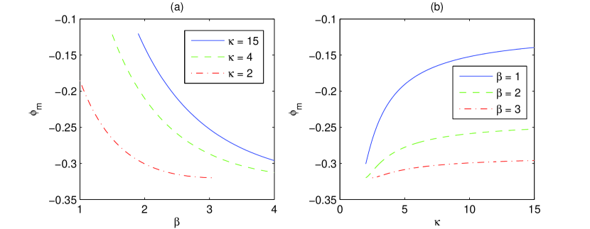
Figure 2.2: Variation of $\phi_{\mathrm{m}}$: (a) with $\beta$ for different values of $\kappa$. Curves from bottom to top: $\kappa=2$ (solid), $4$ (dashed), $15$ (dot-dashed). (b) with $\kappa$ for different values of $\beta$. Curves from top to bottom: $\beta=1$ (solid), $2$ (dashed), $3$ (dot-dashed curve). Here, the Mach number is $0.8$.

Figure 2.3: (a) Variation of pseudopotential $\Psi(\phi)$ with $\phi$ for different density ratio $\beta$. (b) Variation of potential $\phi$ with $\xi$ for different density ratio $\beta$. Curves from top to bottom: $\beta=1.1$ (solid), $1.2$ (dashed), $1.3$ (dot-dashed curve). Here, $\kappa=3$ and $M=1$.

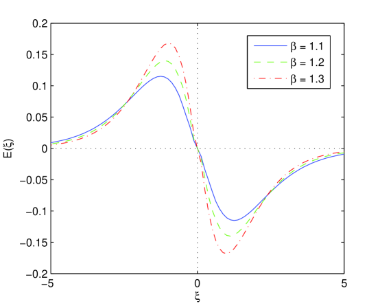
Figure 2.4: Variation of electric field of the EAWs $E(\xi)$ with $\xi$ for different density ratio $\beta$. Curves from bottom to top: $\beta=1.1$ (solid), $1.2$ (dashed), $1.3$ (dot-dashed curve). Here, parameters are same as used in Fig. 2.3.

2.4 Existence Conditions for Solitons

To obtain the electron-acoustic solitons, the conditions for the existence of solitons, namely $\Psi_{1}^{\prime}(\phi,M,\beta,\kappa)=0$ and $\Psi_{1}^{\prime\prime}(\phi,M,\beta,\kappa)<0$ at $\phi=0$, must be satisfied (physically, $\phi=0$ is equilibrium; the potential $\Psi$ needs to have a maximum, an unstable fixed point, at equilibrium; see Fig. 2.3a). The lower limit for the Mach number is then obtained from the condition

$$F_{1}(M,\beta,\kappa)\equiv-\left.\Psi_{1}^{\prime\prime}(\phi,M,\beta,\kappa)\right|_{\phi=0}=\frac{\beta(\kappa-\frac{1}{2})}{\kappa-\tfrac{3}{2}}-\frac{1}{M^{2}}>0.$$ (2.31)

Eq. (2.31) in terms of the Mach number defines a critical value as a lower limit for $M$, i.e.

$$M_{1}(\beta,\kappa)=\left(\frac{\kappa-\tfrac{3}{2}}{\beta(\kappa-\frac{1}{2})}\right)^{1/2}.$$ (2.32)

Soliton solutions may exist only for values of the Mach number $M>M_{1}(\beta,\kappa)$ (lower limit). We notice that $M_{1}$ depends on the parameters $\beta$ and $\kappa$. Figure 2.5 (a) illustrates the modification in the existence domains for different values of $\kappa$.

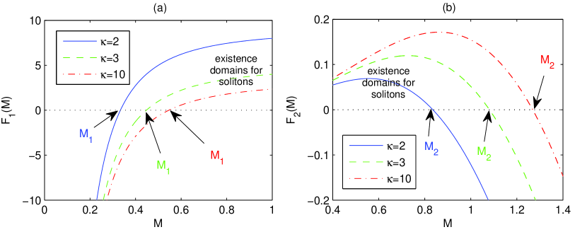
Figure 2.5: The existence domains for stationary solitary structures: (a) the lower limit ($M_{1}$), (b) the upper limit ($M_{2}$). Curves from top to bottom: $\kappa=2$ (solid), $3$ (dashed), $10$ (dot-dashed curve). Here, $\beta=3$, and the quantities $F_{1}$ and $F_{2}$ are defined in (2.31) and (2.33).

We obtain the largest possible value of $M$ through $\Psi_{1}(\phi,M,\beta,\kappa)>0$ at $\phi=\phi_{\max}=-M^{2}/2$. This leads to the following equation:

$$F_{2}(M,\beta,\kappa)\equiv M^{2}\left(1-\dfrac{1}{2}(1+\beta)\right)+\beta\left(1-\left(1+\frac{M^{2}}{2\kappa-3}\right)^{-\kappa+3/2}\right)>0.$$ (2.33)

The upper limit of the Mach number $M$ (say, $M_{2}(\beta,\kappa)$) is thus obtained by solving the associated equation. As illustrated in Fig. 2.5 (b), the upper limit for the Mach number depends on the parameter $\kappa$. From Eq. (2.33), the upper limit ($M_{2}$) is obviously modified by the density ratio $\beta$.

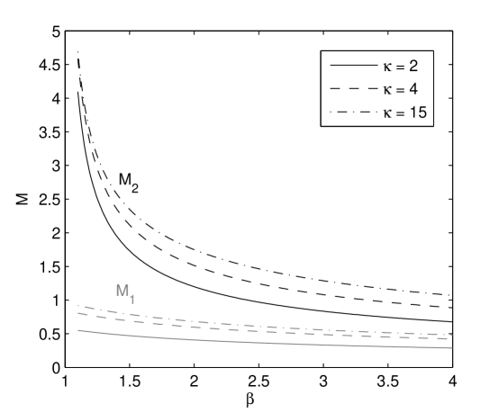
Figure 2.6: Negative potential soliton existence domain in the parameter space of $\beta$ and Mach number $M$. Solitons may be supported in the region between $M_{1}(\beta)$ (gray curve) and $M_{2}(\beta)$ (black curve). It shows variation of $M_{1}(\beta)$ and $M_{2}(\beta)$ with $\beta$ for different values of $\kappa$. Curves from bottom to top: $\kappa=2$ (solid), $4$ (dashed), $15$ (dot-dashed curve).

2.4.1 Hot Suprathermal Effect on Velocity Range

The existence domain is therefore derived from solving $F_{1}(M,\beta,\kappa)>0$ and $F_{2}(M,\beta,\kappa)>0$. As illustrated in Fig. 2.5, $M_{1}$ and $M_{2}$ increase with the increase in the parameter $\kappa$. The range of Mach number ($M_{1}<M<M_{2}$) are shown in Fig. 2.6, as function of equilibrium density ratio $\beta$ with the various $\kappa$. As the density of the hot suprathermal electrons is increased, the lower and upper limits of the Mach number decline. Hence, the increase in the hot electrons causes the existence domain for stationary solitary structure to become dramatically narrow. The minimum Mach number, $M_{1}$, is generally less than the value of $1$. Especially, for the large density ratio, $\beta>2.5$, the Maximum Mach number, $M_{2}$ becomes less than $1.5$ as shown in Fig. 2.6.

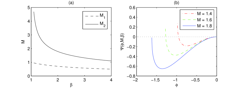
Figure 2.7: EAWs in a plasma with hot Maxwellian electrons ($\kappa\rightarrow\infty$). (a) Soliton existence domain in the parameter space of $\beta$ and Mach number $M$. Solitons may be supported in the region between $M_{1}(\beta)$ (dashed curve) and $M_{2}(\beta)$ (solid curve). (b) Variation of $\Psi_{1}(\phi,M,\beta)$ for $\beta=2$ and different values of Mach number, $M$. Curves from top to bottom: $M=1.2$ (dotted), $M=1.4$ (dot-dashed), $M=1.6$ (dashed), and $M=1.8$ (solid).

2.4.2 Velocity Range in Maxwellian vs. Suprathermal Plasmas

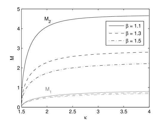
Figure 2.8: Soliton existence domain in the parameter space of $\kappa$ and Mach number $M$. Solitons may be supported in the region between $M_{1}$ (gray curve) and $M_{2}$ (black curve). Curves from top to bottom: $\beta=1.1$ (solid), $1.3$ (dashed), $1.5$ (dot-dashed curve). In the limit $\kappa\rightarrow 3/2$ easily see that $M_{1}=M_{2}=0$.

In the Maxwellian distributions for the hot electrons ($\kappa\rightarrow\infty$), Eq. (2.31) takes the following form

$$F_{1}(M,\beta)=\beta-\frac{1}{M^{2}}>0.$$ (2.34)

This means that the lower limit becomes $M_{1}(\beta)=(\beta)^{-1/2}$. Eq. (2.33) tends to an exponential form

$$F_{2}(M,\beta)=M^{2}\left(1-\dfrac{1}{2}(1+\beta)\right)+\beta\left(1-\exp(-\tfrac{1}{2}M^{2})\right)>0.$$ (2.35)

The above equation solves the upper limit $M_{2}(\beta)$. Negative potential solitary wave solutions of the cold electron fluid system of equations exist for values of the Mach number $M$ in the range $M_{1}(\beta)<M<M_{2}(\beta)$, which depends on the density ratios of the hot electrons to the cold electrons. In Figure 2.7 (a), we have plotted the lower and upper limits, $M_{1}$ and $M_{2}$, respectively, over the range $1.1<\beta<4$ in the limit $\kappa\rightarrow\infty$, and hence show the permitted range of Mach numbers for the electron-acoustic solitons in the Maxwellian distributions. As illustrated in Fig. 2.7 (b) for the Maxwellian distributions, the maximum electrostatic potential of the negative solitary structure increases with the growth in the Mach number $M$ within the existence range $M_{1}<M<M_{2}$. Furthermore, we can see that $M_{1}=M_{2}=0$ in the limit $\kappa\rightarrow 3/2$, as shown in Fig. 2.8.

3 Warm Electron Fluid Model: Temperature Effects

In this chapter, we consider a collisionless and unmagnetized plasma consisting of cool ($T_{c}\neq 0$) inertial electrons, hot suprathermal electron, and inertialess ions. We extend the thermal pressure to the model described in §2. In §3.1, we obtain the linear dispersion relation through using small deviations from the equilibrium state. In §3.2, we investigate the existence domain of the electron-acoustic solitary waves.

The continuity equations of the cool electron fluid can be written as

$$\frac{\partial n_{c}}{\partial t}+\frac{\partial(n_{c}u_{c})}{\partial x}=0.$$ (3.1)

Due to the thermal pressure of the cool electrons, the equation of momentum contains an extra term (compare to Eq. (2.2))

$$\frac{\partial u_{c}}{\partial t}+u_{c}\frac{\partial u_{c}}{\partial x}=\frac{e}{m_{e}}\frac{\partial\phi}{\partial x}-\frac{1}{m_{e}n_{c}}\frac{\partial P_{c}}{\partial x}.$$ (3.2)

The pressure of the cool electrons is given by

$$\frac{\partial P_{c}}{\partial t}+u_{c}\frac{\partial P_{c}}{\partial x}+\gamma P_{c}\frac{\partial u_{c}}{\partial x}=0,$$ (3.3)

where $P_{c}$ is the thermal pressure of the cool electrons, $\gamma=f+2/f\mathit{}$denotes the specific heat ratio, and $f$ denotes the number of degree of freedom, e.g., $\gamma=3$ in the one-dimensional case, also $\gamma=1$ in an adiabatic evolution. We define the temperature ratio of the cool electrons to the hot electrons as $\sigma=T_{c}/T_{h}$. The suprathermal hot electron, fluid cool electrons and uniform ions are linked to the wave potential by the Poisson’s equation (2.3).

The normalized one-dimensional ($\gamma=3$) model equations are written as

$$\frac{\partial n}{\partial t}+\frac{\partial(nu)}{\partial x}=0,$$ (3.4)

$$\frac{\partial u}{\partial t}+u\frac{\partial u}{\partial x}=\frac{\partial\phi}{\partial x}-\frac{\sigma}{n}\frac{\partial P}{\partial x},$$ (3.5)

$$\frac{\partial P}{\partial t}+u\frac{\partial P}{\partial x}+3P\frac{\partial u}{\partial x}=0,$$ (3.6)

$$\frac{\partial^{2}\phi}{\partial x^{2}}=-(\beta+1)+n+\beta\left(1-\frac{\phi}{(\kappa-\tfrac{3}{2})}\right)^{-\kappa+1/2}.$$ (3.7)

The density $n_{c}$ are normalized with the unperturbed density ($n_{c,0}$), the velocity $u_{c}$ with the hot electron thermal velocity ($c_{h,s}=\left(k_{B}T_{h}/m_{e}\right)^{1/2}$), time with the inverse cool electron plasma frequency, $\omega_{pc}^{-1}$, where $\omega_{pc}=(n_{c,0}e^{2}/\varepsilon_{0}m_{e})^{1/2}$, length with the characteristic length scale, $\lambda_{0}=(\varepsilon_{0}k_{B}T_{h}/n_{c,0}e^{2})^{1/2}$, the wave potential $\phi$ with $k_{B}T_{h}/e$, and the thermal pressures with $n_{c,0}k_{B}T_{c}$.

3.1 Dispersion Relation

Let $S=(n,P,u,\phi)$ be any of the system variables describing the system’s state at a given position $x$ and instant $t$. We shall consider small deviations from the equilibrium state $S^{(0)}=(1,1,0,0)$. Using the harmonic wave definition (2.12), and the temporal and spatial derivatives of the first order amplitudes, Eq. (2.13), we get the expressions for density, velocity, and pressure, namely

$$\begin{array}[c]{ccc}n_{1}^{(1)}=\dfrac{k}{\omega}u_{1}^{(1)},\text{ }&u_{1}^{(1)}=-\dfrac{k}{\omega}\left(\phi_{1}^{(1)}-\sigma P_{1}^{(1)}\right),&\text{ }P_{1}^{(1)}=3n_{1}^{(1)}.\end{array}$$ (3.8)

The density in terms of potential are written as

$$n_{1}^{(1)}=-\left(\dfrac{k^{2}}{\omega^{2}-3\sigma k^{2}}\right)\phi_{1}^{(1)}.$$ (3.9)

The system is closed by the Poisson’s equation

$$-k^{2}\phi_{1}^{(1)}=-(\beta+1)+1+n_{1}^{(1)}+\beta\left(1-\frac{\phi_{1}^{(1)}}{\kappa-\tfrac{3}{2}}\right)^{-\kappa+1/2}.$$ (3.10)

Let us expand the $\kappa$-distribution as Eq. (2.16), keeping up to first order. Combining Eqs. (3.9) and (3.10), we get

$$-k^{2}\phi_{1}^{(1)}=-\left(\dfrac{k^{2}}{\omega^{2}-3\sigma k^{2}}\right)\phi_{1}^{(1)}+\beta\left(\frac{\kappa-\frac{1}{2}}{\kappa-\tfrac{3}{2}}\right)\phi_{1}^{(1)}.$$ (3.11)

After a simplification, we recover the linear dispersion relation for the electron-acoustic waves propagating in the warm model:

$$\omega_{2}^{2}=\frac{k^{2}}{k^{2}+k_{D}^{2}}+3{\sigma}k^{2}.$$ (3.12)

where $\sqrt{3{\sigma}}$ is the normalized thermal velocity. We note that $\omega_{2}^{2}(k)=\omega_{1}^{2}(k)+3{\sigma}k^{2}$, where $\omega_{1}$ the cold model frequency defined by Eq. (2.17), and the warm model frequency $\omega^{2}$ as in Eq. (3.12).

Restoring dimensions, the warm model dispersion relation is derived as

$$\omega_{2}^{2}=\omega_{pc}^{2}\frac{k^{2}\lambda_{Dh}^{2}}{k^{2}\lambda_{Dh}^{2}+\left(\dfrac{\kappa-\frac{1}{2}}{\kappa-\tfrac{3}{2}}\right)}+3\sigma k^{2}c_{h,s}^{2}.$$ (3.13)

For the limit $k\ll k_{D}$ Eq. (3.13) reduces to $\omega\simeq kv_{ph}$ where $v_{ph}$ is the phase speed given by

$$v_{ph}\simeq\left(\beta^{-1}\left(\frac{\kappa-\tfrac{3}{2}}{\kappa-\frac{1}{2}}\right)+3\sigma\right)^{1/2}c_{h,s}.$$ (3.14)

The thermal pressure manifests its physical effect in a small modification on the $k$–$\omega$ plane. The linear dispersion relation is affected by the thermal pressure.

3.1.1 Temperature Effect on Linear Waves

Figure 3.1 shows that the slope of the $\omega(k)$ curve increases with a rise in the temperature ratio $\sigma$. Comparing Eqs. (2.21) and (3.14) we can see that growing $\sigma=T_{c}/T_{h}$ increases the phase speed. It is obvious that in the limit $\sigma\rightarrow 0$, Eq. (2.17), the cold model dispersion relation, is given.

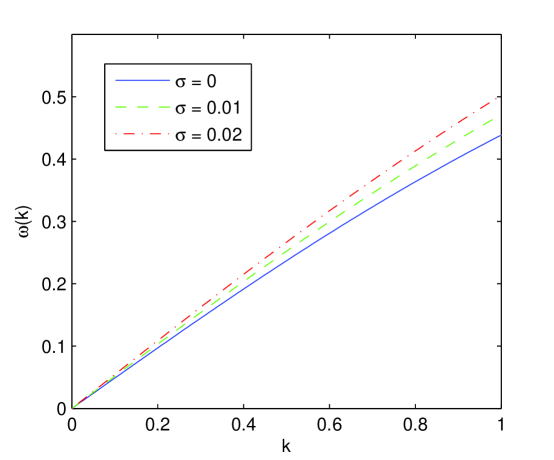
Figure 3.1: Variation of the dispersion function curve for different values of $\sigma$, $\beta=3$, and $\kappa=4$. Curves from bottom to top: $\sigma=0$ (solid), $0.01$ (dashed), $0.02$ (dot-dashed curve).

3.2 Sagdeev Pseudopotential Method

We take Eqs. (3.4)–(3.7) to be stationary in a frame traveling with velocity $M$ (the Mach number). Using the transformation $\xi=x-Mt$, all temporal and spatial derivatives shall be replaced as Eq. (2.22), so Eqs. (3.4)–(3.7) take the following form:

$$-M\dfrac{dn}{d\xi}+\frac{d(nu)}{d\xi}=0,$$ (3.15)

$$-M\dfrac{du}{d\xi}+u\dfrac{du}{d\xi}=\dfrac{d\phi}{d\xi}-\frac{\sigma}{n}\dfrac{dP}{d\xi},$$ (3.16)

$$-M\dfrac{dP}{d\xi}+u\dfrac{dP}{d\xi}+3P\dfrac{du}{d\xi}=0,$$ (3.17)

$$\frac{d^{2}\phi}{d\xi^{2}}=-(\beta+1)+n+\beta\left(1-\frac{\phi}{(\kappa-\tfrac{3}{2})}\right)^{-\kappa+1/2}.$$ (3.18)

Comparing Eqs. (3.15)–(3.18) with Eqs.(2.23)–(2.25), we see a thermal pressure in momentum equation that classifies the propagation velocity as faster or slower than the electron thermal velocity.

Applying the appropriate boundary conditions, namely $n=1$, $P=1$, $u=0$, and $\phi=0$, and integrating the equation of continuity, the equation of motion, and the equation of state provide

$$\begin{array}[c]{cc}u=M(1-\dfrac{1}{n}),\text{ }&u={M-(M}^{2}{+2\phi-3n^{2}\sigma+3\sigma)}^{1/2},\end{array}$$ (3.19)

$$P=n^{3}\rightarrow dP=3n^{2}dn.$$ (3.20)

Combining Eqs. (3.19) and (3.20), we obtain the following solutions through the biquadratic equation (see Appendix C for more detail):

$${n=}\dfrac{1}{2}\left(n_{(+)}\pm n_{(-)}\right),$$ (3.21)

$$\begin{array}[c]{cc}n_{(+)}{\equiv}\left(\dfrac{{2\phi+}\left({M+}\sqrt{3{\sigma}}\right)^{2}}{3{\sigma}}\right)^{1/2},\text{ }&n_{(-)}{\equiv}\left(\dfrac{{2\phi+\left({M-}\sqrt{3{\sigma}}\right)^{2}}}{3{\sigma}}\right)^{1/2}.\end{array}$$ (3.22)

In Eq. (3.21), the upper sign ($+$) is for subsonic cool electrons (${M<}\sqrt{3{\sigma}}$) soliton while the lower sign ($-$) is for supersonic cool electrons (${M>}\sqrt{3{\sigma}}$), because it must satisfy the condition at equilibrium ($n=1$ at $\phi=0$). We notice that the normalized density has two regions in the Mach number domain, namely subsonic and supersonic for hot species and cool species, respectively. We obtain the condition at equilibrium ($n=1$) at $\phi=0$. In the limit $\sigma\rightarrow 0$, we recover the cold limit expression (2.27). To have the real solution, ${2\phi+\left({M-}\sqrt{3{\sigma}}\right)^{2}>0}$, so it yields $\phi_{\max}=-\frac{1}{2}\left({M-}\sqrt{3{\sigma}}\right)^{2}$ to the negative solitary structures.

Substituting the density expression (3.21) into the Poisson’s equation (3.18) leads to the equation of motion:

$$\frac{d^{2}\phi}{d\xi^{2}} =-\Psi_{2}^{\prime}(\phi,M,\beta,\kappa,{\sigma})=-(\beta+1)+\beta\left(1-\frac{\phi}{(\kappa-\tfrac{3}{2})}\right)^{-\kappa+1/2}$$

$$+\dfrac{1}{2\sqrt{3{\sigma}}}\left(\left[{2\phi+}\left({M+}\sqrt{3{\sigma}}\right)^{2}\right]^{1/2}\pm\left[{2\phi+\left({M-}\sqrt{3{\sigma}}\right)^{2}}\right]^{1/2}\right).$$ (3.23)

The above equation can be integrated to yield the energy balance equation:

$$\frac{1}{2}\left(\frac{d\phi}{d\xi}\right)^{2}+\Psi_{2}(\phi,M,\beta,\kappa,{\sigma})=0,$$ (3.24)

where the Sagdeev pseudopotential $\Psi_{1}(\phi,M,\beta,\kappa,{\sigma})$ reads as

$$\Psi_{2}(\phi,M,\beta,\kappa,{\sigma}) =(1+\beta)\phi+\beta\left(1-\left(1+\frac{\phi}{-\kappa+\tfrac{3}{2}}\right)^{-\kappa+3/2}\right)$$

$$+\frac{1}{6\sqrt{3{\sigma}}}\left(\left({M+}\sqrt{3{\sigma}}\right)^{3}\pm{{\left({M-}\sqrt{3{\sigma}}\right)^{3}}}\right.$$

$$-\left.\left[{2\phi+}\left({M+}\sqrt{3{\sigma}}\right)^{2}\right]^{3/2}\mp{\left[{2\phi+\left({M-}\sqrt{3{\sigma}}\right)^{2}}\right]}^{3/2}\right).$$ (3.25)

Here, the upper sign is for subsonic soliton and the lower sign for supersonic. It is easily seen that we get the cold model in the limit $\sigma\rightarrow 0$, i.e., $\lim_{\sigma\rightarrow 0}\Psi_{2}(\phi,M,\beta,\kappa,{\sigma})=\Psi_{1}(\phi,M,\beta,\kappa)$.

3.2.1 Temperature Effect on EAWs

We have numerically solved Eq. (3.25) for a plasma which consists of cool electrons and hot suprathermal electrons. Figure 3.2 (a) shows the variation of Sagdeev pseudopotential $\Psi_{2}(\phi)$ with normalized potential for different temperature ratio $\sigma$. Figure 3.2 (b) shows the variation of solitary waves for the cool electrons for different values of the temperature ratio $\sigma=T_{c}/T_{h}$ as shown on the curves for $\beta=1.1$, $\kappa=3$ and Mach number, $M=1$. The amplitude of the wave potential decreases with the increase in $\sigma$. The associated bipolar electric field structures are shown in Fig. 3.3. We can see a decline in the electric field structures with an increase in the thermal velocity $\sqrt{3\sigma}$. As illustrated in Fig. 3.4, the number density and the velocity of the cool electrons decline with the growth in the thermal velocity.

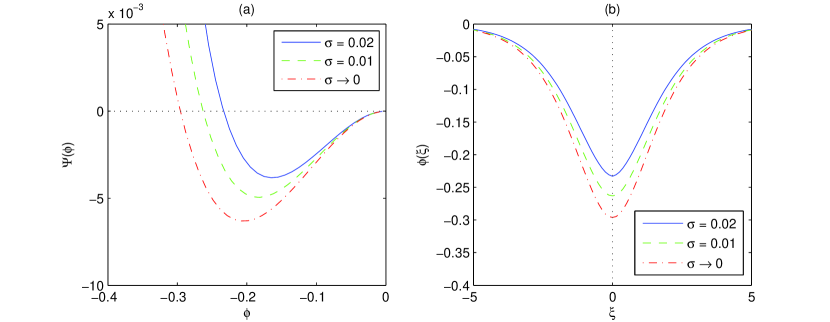
Figure 3.2: (a) Variation of pseudopotential $\Psi(\phi)$ with $\phi$ for different temperature ratio $\sigma$. (b) Variation of the electron-acoustic potential $\phi$ with $\xi$ for different temperature ratio $\sigma$. Curves from bottom to top: $\sigma\rightarrow 0$ (dot-dashed curve), $\sigma=0.01$ (dashed), $0.02$ (solid). Here, $\beta=1.1$, $\kappa=3$ and $M=1$.

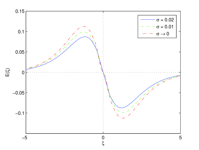
Figure 3.3: Variation of electric field of the EAWs $E(\xi)$ with $\xi$ for different temperature ratio $\sigma$. Curves from top to bottom: $\sigma\rightarrow 0$ (dot-dashed curve), $\sigma=0.01$ (dashed), $0.02$ (solid). Here, parameters are same as used in Fig. 3.2.

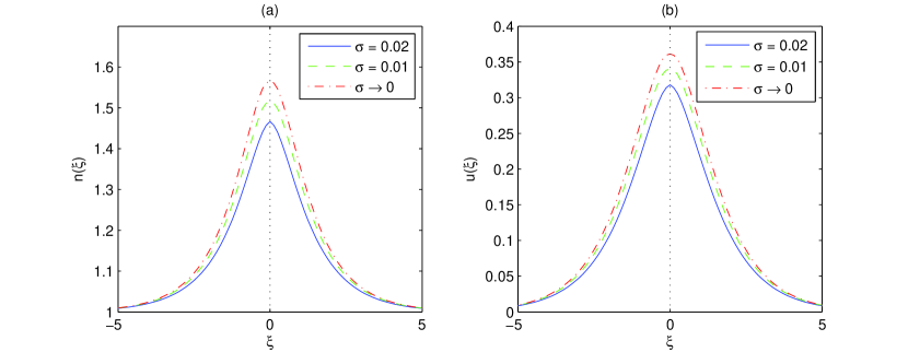
Figure 3.4: (a) Variation of density $n$ with $\xi$ for different temperature ratio $\sigma$. (b) Variation of velocity $u$ with $\xi$ for different temperature ratio $\sigma$. Curves from top to bottom: $\sigma\rightarrow 0$ (dot-dashed curve), $\sigma=0.01$ (dashed), $0.02$ (solid). Here, parameters are same as used in Fig. 3.2.

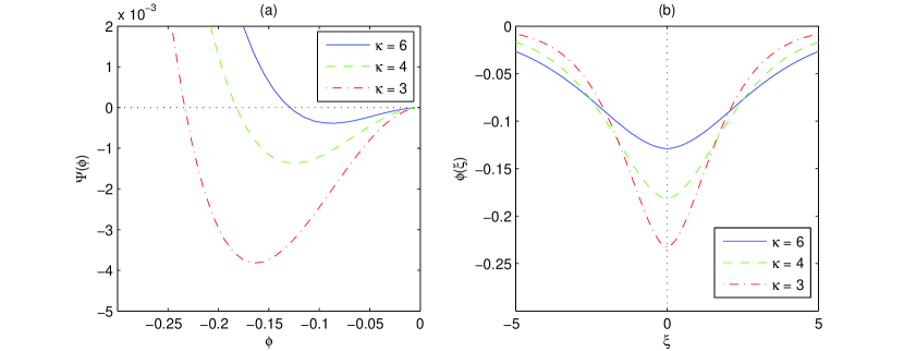
Figure 3.5: (a) Variation of pseudopotential $\Psi(\phi)$ with $\phi$ for different $\kappa$. (b) Variation of potential $\phi$ with $\xi$ for different $\kappa$. Curves from bottom to top: $\kappa=6$ (solid), $4$ (dashed), $3$ (dot-dashed curve). Here, $\sigma=0.02$, $\beta=1.1$, and $M=1$.

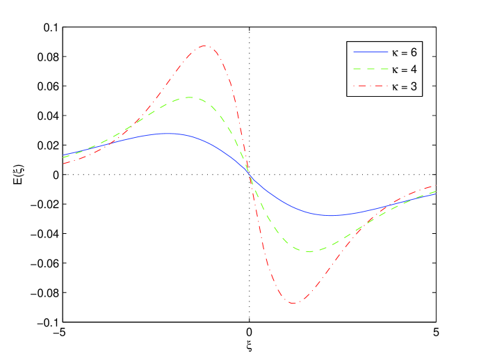
Figure 3.6: Variation of electric field of the EAWs $E(\xi)$ with $\xi$ for different $\kappa$. Curves from top to bottom: $\kappa=6$ (solid), $4$ (dashed), $3$ (dot-dashed curve). Here, parameters are same as used in Fig. 3.5.

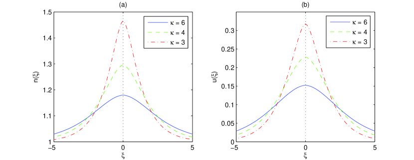
Figure 3.7: (a) Variation of density $n$ with $\xi$ for different $\kappa$. (b) Variation of velocity $u$ with $\xi$ for different $\kappa$. Curves from top to bottom: $\kappa=6$ (solid), $4$ (dashed), $3$ (dot-dashed curve). Here, parameters are same as used in Fig. 3.5.

3.2.2 Suprathermal Effect on EAWs

Figure 3.5 (a) shows the variation of Sagdeev pseudopotential $\Psi_{2}(\phi)$ versus $\phi$ for different $\kappa$. The absolute maximum electrostatic potential $|\phi_{\mathrm{m}}|$ decrease with the rise in $\kappa$, while the large $\kappa$ turns into Maxwellian distribution. The value of $\kappa$ between $3/2$ and $6$ effectively describe the solitary structure of the electron-acoustic wave in a suprathermal plasma. Figure 3.6 shows the variation of the associated bipolar electric field structures for different values of $\kappa$. In Fig. 3.7, we can see the density $n$ and the velocity $u$ increase, as the parameter $\kappa$ is decreased.

3.3 Soliton Existence

We require to find out if the conditions for the existence of solitons are satisfied for Eq. (3.25), i.e., $\Psi_{2}^{\prime}(\phi,M,\beta,\kappa,{\sigma})=0$ and $\Psi_{2}^{\prime\prime}(\phi,M,\beta,\kappa,{\sigma})<0$ at $\phi=0$. We derive the lower limit for the existence domain from the condition

$$F_{1}(M,\beta,\kappa,{\sigma})=-\left.\Psi_{2}^{\prime\prime}(\phi,M,\beta,\kappa,{\sigma})\right|_{\phi=0}=\frac{\beta(\kappa-\frac{1}{2})}{\kappa-\tfrac{3}{2}}-\frac{1}{M^{2}-3{\sigma}}>0.$$ (3.26)

Eq. (3.26) provides the minimum value for the Mach number:

$$M_{1}(\beta,\kappa,{\sigma})=\left(\frac{\kappa-\tfrac{3}{2}}{\beta(\kappa-\frac{1}{2})}+3{\sigma}\right)^{1/2}.$$ (3.27)

Soliton solutions may exist only for the Mach number greater than $M_{1}(\beta,\kappa,{\sigma})$. We can see that $M_{1}$ depends on the parameters $\beta$, $\kappa$, and $\sigma$. This shows that electron thermal effects increase the Mach number threshold. In the limit $\sigma\rightarrow 0$, it provides the expression for cold model (2.32).

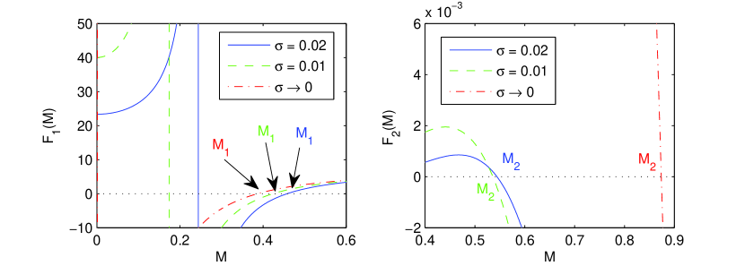
Figure 3.8: The existence domains for stationary solitary structures: (a) the lower limit ($M_{1}$), (b) the upper limit ($M_{2}$). Curves: $\sigma\rightarrow 0$ (dot-dashed curve), $\sigma=0.01$ (dashed), $0.02$ (solid). Here, $\beta=4$ and $\kappa=3$. The quantities $F_{1}$ and $F_{2}$ are defined in (3.26) and (3.28)

We obtain the largest possible value of $M$ through $F_{2}(M,\beta,\kappa,{\sigma})$ = $\Psi_{2}(\phi,M,$ $\beta,\kappa,{\sigma})|_{\phi=\phi_{\max}}>0$. This yields the following equation:

$$F_{2}(M,\beta,\kappa,{\sigma}) =-\frac{1}{2}(1+\beta)\left({M-}\sqrt{3{\sigma}}\right)^{2}+M{{{}^{2}+}\sigma}-\frac{4}{3}M\sqrt{M\sqrt{3{\sigma}}}$$

$$+\beta\left(1-\left(1+\frac{\left({M-}\sqrt{3{\sigma}}\right)^{2}}{2\kappa-3}\right)^{-\kappa+3/2}\right).$$ (3.28)

Solving Eq. (3.28) provides the upper limit $M_{2}(\alpha,\kappa)$ for the Mach number. Figure 3.8 illustrates a modification in the existence domains ($M_{1}<M<M_{2}$) for different values of $\sigma$. We find out that “cool”electrons need to be supersonic (in the sense ${M>}\sqrt{3{\sigma}}$) and “hot”suprathermal electrons subsonic (${M<}\sqrt{3{\sigma}}$) [38, 39, 40]. Negative solitary structures of the cool electron-fluid may be found in the range $M_{1}<M<M_{2}$, which depends on the parameters $\beta$, $\kappa$, and $\sigma$.

3.3.1 Velocity Range in Maxwellian vs. Suprathermal Plasmas

In the Maxwellian distributions ($\kappa\rightarrow\infty$), we get

$$F_{1}(M,\beta,{\sigma})=\beta-\frac{1}{M^{2}-3{\sigma}}>0.$$ (3.29)

$$F_{2}(M,\beta,{\sigma}) =-\frac{1}{2}(1+\beta)\left({M-}\sqrt{3{\sigma}}\right)^{2}+M{{{}^{2}+}\sigma}-\frac{4}{3}M^{3/2}\left(3{\sigma}\right)^{1/4}$$

$$+\beta\left(1-\exp(-\tfrac{1}{2}\left({M-}\sqrt{3{\sigma}}\right)^{2})\right).$$ (3.30)

The above equation solves the upper limit $M_{2}(\beta)$, while the lower limit becomes $M_{1}(\beta,{\sigma})=\left(1/\beta+3{\sigma}\right)^{1/2}$. As shown in Figures 3.9–3.11, growing the thermal pressure pushes up the lower limit $M_{1}$, but turns down the upper limit $M_{2}$ of the Mach number. We can also see the decline in both $M_{1}$ and $M_{2}$ with the increase in $\beta$ and decrease in $\kappa$, which has been previously described in §2.4.

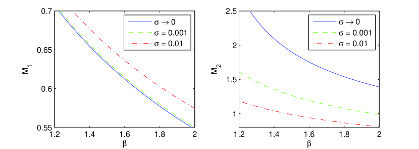
Figure 3.9: Variation of the lower limit $M_{1}$ and the upper limit $M_{2}$ with $\beta$ for different temperature ratio $\sigma$. Curves from bottom to top: $\sigma\rightarrow 0$ (solid), $\sigma=0.001$ (dashed), $0.01$ (dot-dashed curve). Here, $\kappa=3$.

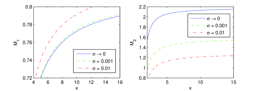
Figure 3.10: Variation of the lower limit $M_{1}$ and the upper limit $M_{2}$ with $\kappa$ for different temperature ratio $\sigma$. Curves from bottom to top: $\sigma\rightarrow 0$ (solid), $\sigma=0.01$ (dashed), $0.001$ (dot-dashed curve). Here, $\beta=1.5$.

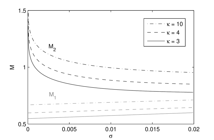
Figure 3.11: Negative potential soliton existence domain in the parameter space of $\sigma$ and Mach number $M$. Solitons may be supported in the region between $M_{1}(\sigma)$ (gray curve) and $M_{2}(\sigma)$ (black curve). It shows variation of $M_{1}(\sigma)$ and $M_{2}(\sigma)$ with $\sigma$. Curves from bottom to top: $\kappa=3$ (solid), $4$ (dashed), $10$ (dot-dashed curve). Here, $\beta=2$.

In the limit $\kappa\rightarrow 3/2$, the lower limit of the Mach number takes the form $M_{1}(\beta,{\sigma})=\sqrt{3{\sigma}}$. It is non-zero, in contrast to the cold model in §2.4 which turned into zero. The upper limit $M_{2}$ can be solved by

$$F_{2}(M,\beta,{\sigma})=-\frac{1}{2}(1+\beta)\left({M-}\sqrt{3{\sigma}}\right)^{2}+M{{{}^{2}+}\sigma}-\frac{4}{3}M^{3/2}\left(3{\sigma}\right)^{1/4}>0.$$ (3.31)

It also appears to be, nonvanishing, in proportion to the thermal velocity, $M_{2}\sim\sqrt{3{\sigma}}$. In the limit $\sigma\rightarrow 0$, we obtain the cold model results ($M_{1}=M_{2}=0$).

3.3.2 Temperature Effect on Velocity Range

The existence condition ($M_{1}<M<M_{2}$) is obtained through $F_{1}(M,\beta,\kappa,{\sigma})>0$ and $F_{2}(M,\beta,\kappa,{\sigma})>0$. Fig. 3.9 shows that $M_{1}$ and $M_{2}$ decline with the increase in the parameter $\beta$, i.e., the density of the hot electrons. We notice the existence domain becomes narrower, as the hot electrons density is increased. The range of the Mach number are shown in Fig. 3.10, as function of $\kappa$ with the various $\sigma$. In this figure, one can see that, moving into the Maxwellian distribution ($\kappa\rightarrow\infty$) will broaden the Mach number range. However, the lower Mach number limit tend to $\sqrt{3{\sigma}}$, and the upper Mach number limit to $\sqrt{3{\sigma}}$ as $\kappa\rightarrow 3/2$, the limiting value of $\kappa$. As illustrated in Fig. 3.11 for suprathermal situation ($3/2<\kappa<6$), the lower Mach number limit, $M_{1}$, is generally less than the value of $0.75$, and the upper Mach number limit, $M_{2}$, for very warm model ($\sigma>0.005$) becomes less than $1$.

4 Two-Fluid Model: Ion Inertia Effects

In this chapter, we consider a collisionless and unmagnetized plasma with three components, namely, cool inertial electrons, inertialess hot suprathermal electrons, and inertial ions. We include the inertial ions in the model described in Chapter 3. We employ the cool electrons described by Eqs. (3.1)–(3.3), the hot suprathermal electrons, assumed to obey the kappa velocity distribution (2.4), and ions, described by the fluid-moment equations. The electron-fluid and ion-fluid are coupled through Poisson’s equation (2.3). In §4.1, we derive the linear dispersion relation from a linear methodology. In §4.2, we develop a Sagdeev pseudopotential method and determine the existence domain of stationary solitary waves.

The fluid equations for the ions read

$$\frac{\partial n_{i}}{\partial t}+\frac{\partial(n_{i}u_{i})}{\partial x}=0,$$ (4.1)

$$\frac{\partial u_{i}}{\partial t}+u_{i}\frac{\partial u_{i}}{\partial x}=-\frac{Ze}{m_{i}}\frac{\partial\phi}{\partial x},$$ (4.2)

where $n_{i,0}$ is the density of the ions in the undisturbed plasma, $m_{e}$ the mass of the ions, $Z$ the number of ions (everywhere, $Z=1$).

The normalized fluid-moment equations of the cool electron and the ions, and the Poisson’s equation are written as Eqs. (3.4)–(3.6), and

$$\frac{\partial\tilde{n}}{\partial t}+\frac{\partial(\tilde{n}\tilde{u})}{\partial x}=0,$$ (4.3)

$$\frac{\partial\tilde{u}}{\partial t}+\tilde{u}\frac{\partial\tilde{u}}{\partial x}=-\mu\frac{\partial\phi}{\partial x},$$ (4.4)

$$\frac{\partial^{2}\phi}{\partial x^{2}}=-\tilde{n}+n+\beta\left(1-\frac{\phi}{(\kappa-\tfrac{3}{2})}\right)^{-\kappa+1/2},$$ (4.5)

All densities are normalized with the unperturbed density of the cool electrons ($n_{c,0}$), all velocities with the hot electron thermal velocity ($c_{h,s}=\sqrt{k_{B}T_{h}/m_{e}}$):

$$\begin{array}[c]{cccc}\dfrac{n_{c}}{n_{c,0}}\rightarrow n,\text{ }&\dfrac{n_{i}}{n_{c,0}}\rightarrow\tilde{n},\text{ }&\dfrac{u_{c}}{c_{h,s}}\rightarrow u,\text{ }&\dfrac{u_{i}}{c_{h,s}}\rightarrow\tilde{u},\end{array}$$ (4.6)

space and time variables are scaled by the characteristic length scale, $\lambda_{0}=\left(\varepsilon_{0}k_{B}T_{h}/n_{c,0}e^{2}\right)^{1/2}$, the inverse cool electron plasma frequency $\omega_{pc}^{-1}$ = $(\varepsilon_{0}m_{e}/$ $n_{c,0}e^{2})^{1/2}$, the potential scale reads $\phi_{0}=k_{B}T_{h}/e$, and the thermal pressures scale $P_{0}=n_{c,0}k_{B}T_{c}$. We also define the mass ratio of electron to ion as $\mu=m_{e}/m_{i}=1/1836$ (proton) and the number of ions as $Z=1$ (Hydrogen).

4.1 Linear Method

Let us assume that $S=(n,u,\tilde{n},\tilde{u},P,\phi)$ be the system variables that describe the system’s state at a given space and time. The small deviations from the equilibrium state are $S^{(0)}=(1,0,1+\beta,0,1,0)$. We use the first-order derivatives of the harmonic wave amplitude as Eq. (2.13), we get the following expressions for velocity, density of the cool electrons and the ions, and thermal pressure,

$$\begin{array}[c]{ccc}n_{1}^{(1)}=\dfrac{k}{\omega}u_{1}^{(1)},\text{ }&u_{1}^{(1)}=-\dfrac{k}{\omega}\left(\phi_{1}^{(1)}-\sigma P_{1}^{(1)}\right),\text{ }&P_{1}^{(1)}=3n_{1}^{(1)},\end{array}$$ (4.7)

$$\begin{array}[c]{cc}\tilde{n}_{1}^{(1)}=\dfrac{k}{\omega}\tilde{u}_{1}^{(1)},\text{ }&\tilde{u}_{1}^{(1)}=\mu\dfrac{k}{\omega}\phi_{1}^{(1)},\end{array}$$ (4.8)

The Poisson’s equation closes all system variables together.

$$-k^{2}\phi_{1}^{(1)}=-\beta-\tilde{n}_{1}^{(1)}+n_{1}^{(1)}+\beta\left(1-\frac{\phi}{(\kappa-\tfrac{3}{2})}\right)^{-\kappa+1/2}.$$ (4.9)

Using the fact that $\mu\ll 1$, we use the Taylor expansion to first order. If we approximate to first order, we obtain the linear dispersion relation $\omega_{3}=\omega_{3}(k)$:

$$\omega_{3}^{2}(k)\simeq\omega_{2}^{2}(k){+}\frac{{\mu k^{2}}}{\left(k^{2}+k_{D}^{2}\right)\left[1+3{\sigma}\left(k^{2}+k_{D}^{2}\right)\right]},$$ (4.10)

where $k_{D}$ is defined by Eq. (2.18), and $\omega_{2}(k)$, the wave frequency of the one-fluid warm model, is given by Eq. (3.12). In the limit $\mu\rightarrow 0$, we get the one-fluid warm model as Eq. (3.12).

4.1.1 Ion Inertia Effects on Linear Waves

To understand how inertial ions affect the linear dispersion function, we may write Eq. (4.10) as follows

$$\omega_{3}^{2}\simeq\left(1+\frac{{\mu}}{1+3{\sigma}\left(k^{2}+k_{D}^{2}\right)}\right)\omega_{1}^{2}+3{\sigma}k^{2}.$$ (4.11)

We see that the thermal effect has an dramatic effect on the results of the inertial ions. Hence, there is extremely small difference between the dispersion curve of this model and the model described in §3, as shown in Fig. 4.1. In the limit $\sigma\rightarrow 0$, we obtain $\omega_{3}\simeq\left(1+{\mu}\right)^{1/2}\omega_{1}\approx\left(1+\frac{1}{2}{\mu}\right)\omega_{1}$, with the result that the electron-acoustic phase speed increases by order of $\frac{1}{2}{\mu}$ (for the Hydrogen $\mu=m_{e}/m_{i}=1/1836$). Figure 4.2 shows the difference between two-fluid warm model ($\sigma=0.02$) and two-fluid cold model ($\sigma=0$). We see that the thermal effect ($\sqrt{3{\sigma}}$) plays a role in modifying the dispersion curve more than the inertial ions (while $\mu\ll 1$). It seems that the inertial ions make some minor effects to the electron-acoustic phase speed.

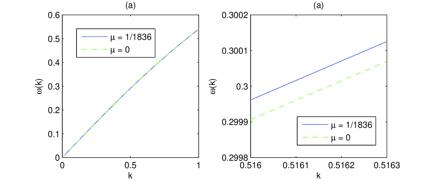
Figure 4.1: Variation of the dispersion function curve for different values of $\mu$. Curves from top to bottom: $\mu=1/1836$ (solid), and $0$ (dashed). Here, $\kappa=3$, $\beta=2$, $\sigma=0.02$, and $Z=1$.

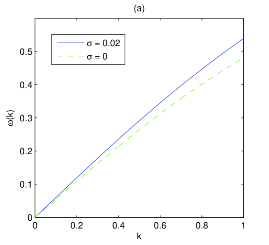
Figure 4.2: Variation of the dispersion function curve for different values of $\sigma$. Curves from top to bottom: $\sigma=0.02$ (solid), and $0$ (dashed). Here, $\kappa=3$, $\beta=2$, $Z=1$, and $\mu=1/1836$.

4.2 Nonlinear Pseudopotential Technique

To investigate the existence of the electron-acoustic solitary waves, we use the pseudopotential approach by assuming that all dependent variables depend on the traveling coordinate $\xi=x-Mt$, where $M$ is the Mach number. Using this transformation, we get Eqs. (3.15)–(3.17), and the ion-fluid equations take the following form:

$$-M\dfrac{d\tilde{n}}{d\xi}+\frac{d(\tilde{n}\tilde{u})}{d\xi}=0,$$ (4.12)

$$-M\dfrac{d\tilde{u}}{d\xi}+\tilde{u}\dfrac{d\tilde{u}}{d\xi}=-\mu\frac{d\phi}{d\xi},$$ (4.13)

$$\frac{d^{2}\phi}{d\xi^{2}}=-\tilde{n}+n+\beta\left(1-\frac{\phi}{(\kappa-\tfrac{3}{2})}\right)^{-\kappa+1/2}.$$ (4.14)

Integrating Eqs. (3.15)–(3.17) and Eqs. (4.12)–(4.13) yield

$$\begin{array}[c]{cc}u=M(1-\dfrac{1}{n}),&u={M-}\left({M}^{2}{+2\phi-3n^{2}\sigma+3\sigma}\right)^{1/2},\end{array}$$ (4.15)

$$\begin{array}[c]{cc}\tilde{u}=M\left(1-\dfrac{(1+\beta}{\tilde{n}}\right),&\tilde{u}=M{-}\left({M}^{2}{-2\mu\phi}\right)^{1/2}.\end{array}$$ (4.16)

Combining Eqs. (4.15)–(4.16), we get

$${n=}\dfrac{1}{2\sqrt{3{\sigma}}}\left(\left[{2\phi+}\left({M+}\sqrt{3{\sigma}}\right)^{2}\right]^{1/2}\pm\left[{2\phi+\left({M-}\sqrt{3{\sigma}}\right)^{2}}\right]^{1/2}\right),$$ (4.17)

$$\tilde{n}=(1+\beta)\left({1-\mu}\frac{{2\phi}}{{M}^{2}}\right)^{-1/2}.$$ (4.18)

The upper/lower sign in Eq. (4.17) is for subsonic/supersonic solitons, respectively. In the limit $\mu\rightarrow 0$, we recover the inertialess ions ($\tilde{n}=1+\beta$). We also obtain the condition at equilibrium ($n=1$ and $\tilde{n}=1+\beta$) through the limit $\phi\rightarrow 0$.

Eq. (4.17) shows that $\phi_{\max}^{(-)}=-\frac{1}{2}\left({M-}\sqrt{3{\sigma}}\right)^{2}$, which is considered to be the maximum (in absolute value) limit for the negative electrostatic wave potential. Meanwhile, two-fluid model, Eq. (4.18), gives a maximum limit for the positive electrostatic wave potential $\phi_{\max}^{(+)}=\frac{1}{{2}}{\mu}^{-1}{{M}^{2}}$. We can see that the maximum limit for the positive solitary waves is in proportion to ${\mu}^{-1}$ (for the proton $\mu^{-1}=1836$). This means that the two-fluid model may support a positive soliton with very large amplitude (by order of ${\mu}^{-1}$) in comparison with negative solitons. However, we must also think of the possible range of the propagation velocity ($M$), which is valid for the positive solitary waves. In the two-fluid model, the positive pulses usually appear to be subsonic ($M<1$), i.e., heavy species (ion) propagating slowly. Hence, we may not observe very large positive pulses due to small velocity ($M\ll 1$).

Substituting equations (4.17) and (4.18) into equation (4.14), we get the equation of motion:

$$\frac{d^{2}\phi}{d\xi^{2}} =-\Psi_{3}^{\prime}(\phi,M,\beta,\kappa,{\sigma},\mu)=-(1+\beta)\left({1-\mu}\frac{{2\phi}}{{M}^{2}}\right)^{-1/2}+\beta\left(1-\frac{\phi}{(\kappa-\tfrac{3}{2})}\right)^{-\kappa+1/2}$$

$$+\dfrac{1}{2\sqrt{3{\sigma}}}\left(\left[{2\phi+}\left({M+}\sqrt{3{\sigma}}\right)^{2}\right]^{1/2}\pm\left[{2\phi+\left({M-}\sqrt{3{\sigma}}\right)^{2}}\right]^{1/2}\right).$$ (4.19)

Multiplying the above equation by $d\phi/d\xi$, integrating, and applying boundary condition, namely $n=1$, $\tilde{n}=1+\beta$, $P=1$, and $u=\tilde{u}=\phi=0$, we find the energy balance equation:

$$\frac{1}{2}\left(\frac{d\phi}{d\xi}\right)^{2}+\Psi_{3}(\phi,M,\beta,\kappa,{\sigma},\mu)=0,$$ (4.20)

where the Sagdeev pseudopotential $\Psi_{3}(\phi,M,\beta,\kappa,{\sigma},\mu)$ is written as

$$\Psi_{3}(\phi,M,\beta,\kappa,{\sigma},\mu) =(1+\beta)\frac{{M}^{2}}{{\mu}}\left(1-\left({1-\mu}\frac{{2\phi}}{{M}^{2}}\right)^{1/2}\right)$$

$$+\beta\left(1-\left(1-\frac{\phi}{\kappa-\tfrac{3}{2}}\right)^{-\kappa+3/2}\right)$$

$$+\frac{1}{6\sqrt{3{\sigma}}}\left(\left({M+}\sqrt{3{\sigma}}\right)^{3}\pm{{\left({M-}\sqrt{3{\sigma}}\right)^{3}}}\right.$$

$$\left.-\left[{2\phi+}\left({M+}\sqrt{3{\sigma}}\right)^{2}\right]^{3/2}\mp{\left[{2\phi+\left({M-}\sqrt{3{\sigma}}\right)^{2}}\right]}^{3/2}\right).$$ (4.21)

In the limit $\mu\rightarrow 0$, we obtain one-fluid warm model, i.e., $\lim_{\mu\rightarrow 0}\Psi_{3}(\phi,M,\beta,\kappa,{\sigma},\mu)=\Psi_{2}(\phi,M,\beta,\kappa,{\sigma})$ as in Eq. (3.25). We also get the cold model from the limit ${\sigma}\rightarrow 0$ (see Eq. (2.17))

4.2.1 Ion Inertia Effects on EA Solitons

As illustrated in Fig. 4.3, the ion-fluid has a trivial role in modifying negative supersonic (${M>}\sqrt{3{\sigma}}$) solitary waves. Figure 4.4 shows the difference between two-fluid model for $\mu=0.1$ and one-fluid model. However, $\mu=0.1$ has not physical mean, and only was used to distinguish between them.

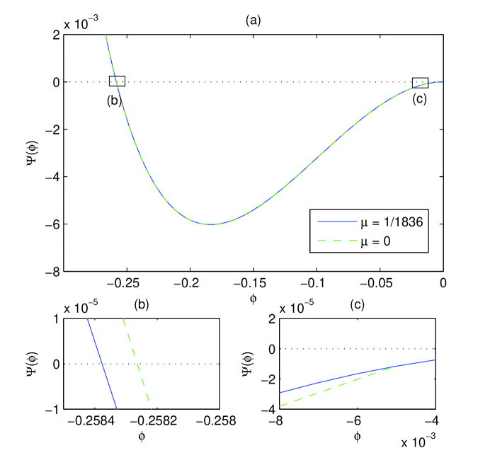
Figure 4.3: (a) Variation of pseudopotential $\Psi(\phi)$ with $\phi$ for $\mu=1/1836$ (solid) and $0$ (dot-dashed curve). As zoomed in on (b) and (c), difference between two curves are extremely small due to small value of $\mu$. Here, $\beta=1.1$, $\kappa=3$, $M=1$, and $Z=1$.

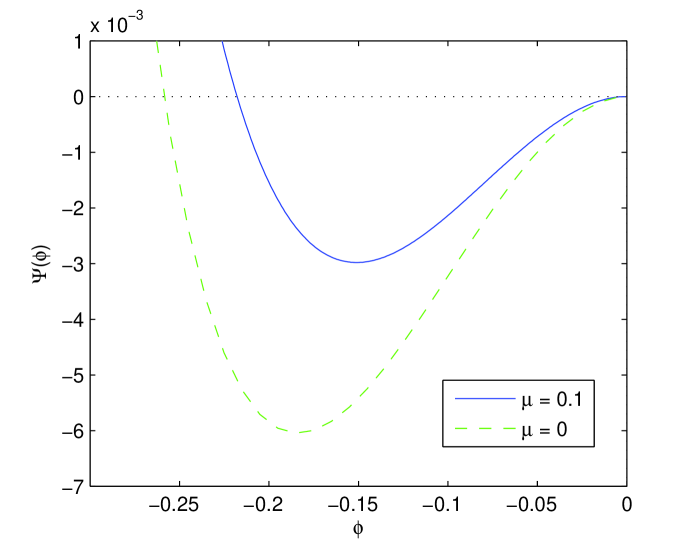
Figure 4.4: Variation of pseudopotential $\Psi(\phi)$ with $\phi$ for different mass ratio $\mu$. Curves from top to bottom: $\mu=0.1$ (solid) and $0$ (dot-dashed curve). Here, $\mu=0.1$ has not physical mean and other parameters are same as used in Fig. 4.3.

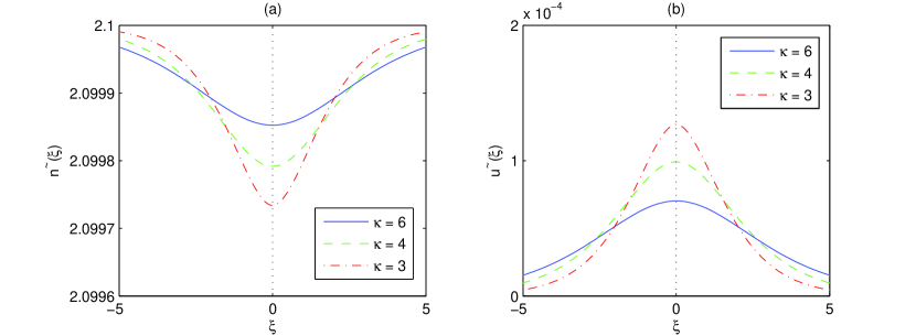
Figure 4.5: (a) Variation of density $\tilde{n}$ with $\xi$ for different $\kappa$. (b) Variation of velocity $\tilde{u}$ with $\xi$ for different $\kappa$. Curves from top to bottom: $\kappa=6$ (solid), $4$ (dashed), $3$ (dot-dashed curve). Here, $\sigma=0.02$, $\beta=1.1$, $M=1$, $Z=1$, and $\mu=1/1836$.

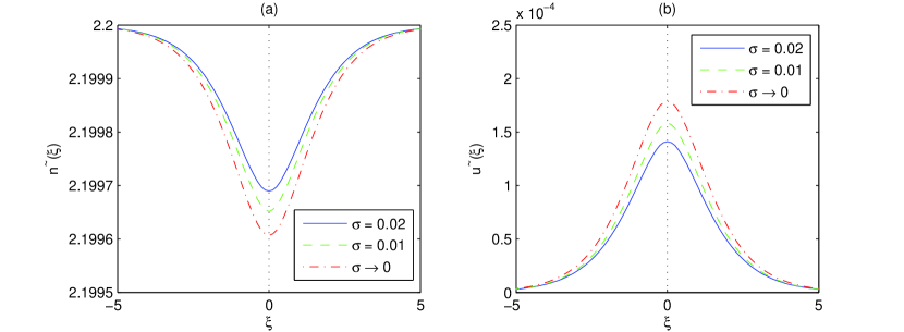
Figure 4.6: (a) Variation of density $\tilde{n}$ with $\xi$ for different temperature ratio $\sigma$. (b) Variation of velocity $\tilde{u}$ with $\xi$ for different temperature ratio $\sigma$. Curves from top to bottom: $\sigma\rightarrow 0$ (dot-dashed curve), $\sigma=0.01$ (dashed), $0.02$ (solid). Here, $\beta=1.1$, $\kappa=3$, $M=1$, $Z=1$, and $\mu=1/1836$.

Numerically solving Eq. (4.21) provides the number density and the velocity of the ions. Figure 4.6 shows the variation of $\tilde{n}$ and $\tilde{u}$ for different temperature ratio $\sigma$ are slight. We see a decline in the absolute ion quantities (density and velocity) with an increase in the thermal velocity $\sqrt{3{\sigma}}$. Figure 4.5 shows the variation of the ion density and the ion velocity for different $\kappa$. We note that, by increasing $\kappa$ (closer to the Maxwellian background), the ion quantities decreases. Hence, the inertial ions are more affect by suprathermal species than the Maxwellian distribution

4.2.2 Positive Solitary Wave Structure

It is interesting to see the subsonic solution ($M<\sqrt{3{\sigma}}$), which is associated with the upper sign in Eq. (4.21). Previously (§3.2), we classified the Mach number under two regions, i.e., subsonic/supersonic for hot/cool species, respectively. The cool electron-fluid can generally support a negative supersonic electrostatic wave. But, ion-fluid may possess a subsonic soliton, which gives a positive pulse. We have numerically solved Eq. (4.21) for the subsonic condition. As illustrated in Fig. 4.7, this makes the positive electrostatic wave potential. We see that the amplitude of pulse rises as the Mach number is increased. Figure 4.8 shows that increasing $\kappa$ (approach the Maxwellian distribution) reduces the positive solitary pulse amplitude, but extends the full width at half maximum (FWHM).

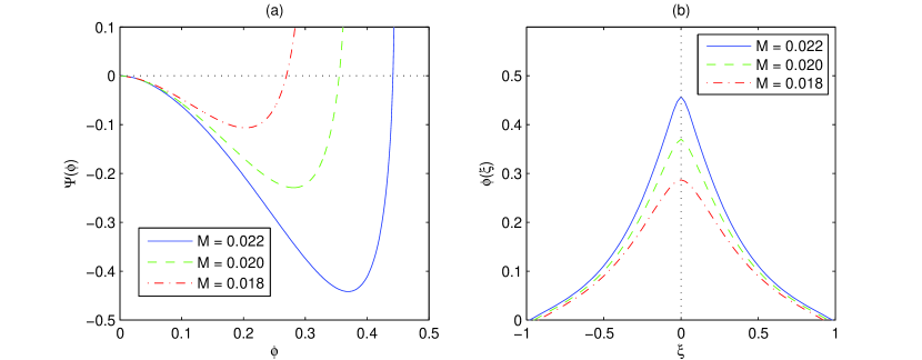
Figure 4.7: Compressive (positive) solitary structures at subsonic region ($M\ll\Theta$). (a) Variation of pseudopotential $\Psi(\phi)$ with $\phi$ for different values of the Mach number $M$. (b) Variation of potential $\phi$ with $\xi$ for different $M$. Curves from top to bottom: $M=0.022$ (solid), $0.020$ (dashed), $0.018$ (dot-dashed curve). Here, $\beta=3$, $\kappa=3$, $\sigma=0.02$, $Z=1$, and $\mu=1/1836$.

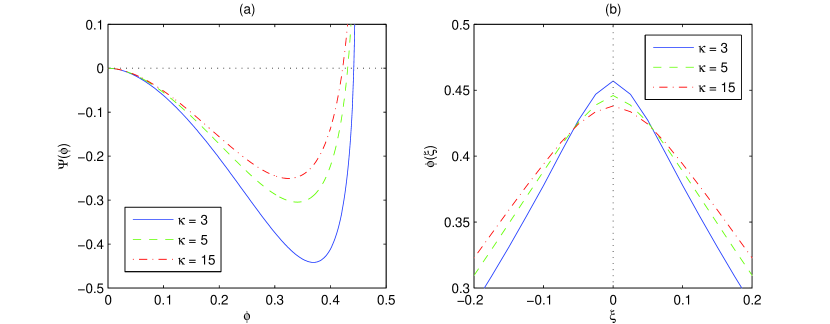
Figure 4.8: Compressive solitary structures at subsonic region. (a) Variation of pseudopotential $\Psi(\phi)$ with $\phi$ for different $\kappa$. (b) Variation of potential $\phi$ with $\xi$ for different $\kappa$. Curves from top to bottom: $\kappa=3$ (solid), $5$ (dashed), $15$ (dot-dashed curve). Here, $M=0.022$, $\beta=3$, $\kappa=3$, $\sigma=0.02$, $Z=1$, and $\mu=1/1836$.

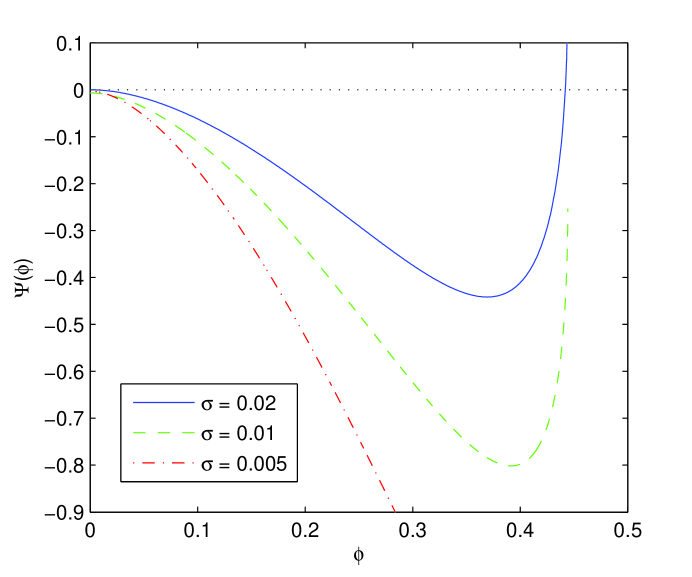
Figure 4.9: Variation of pseudopotential $\Psi(\phi)$ with $\phi$ for different temperature ratio $\sigma$. Curves from bottom to top: $\sigma=0.02$ (solid), $\sigma=0.01$ (dashed), $0.005$ (dot-dashed curve). Here, $M=0.022$, $\beta=3$, $\kappa=3$, $Z=1$, and $\mu=1/1836$.

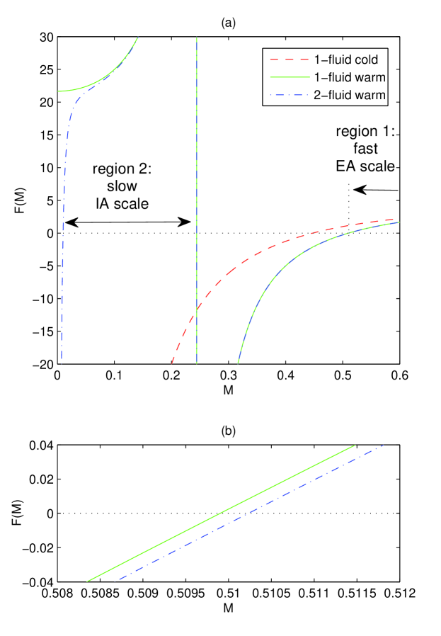
Figure 4.10: The existence domains for stationary solitary structures. The quantities $F_{1}$ for 1-fluid cold model (dashed curve), 1-fuild warm model (solid), and 2-fluid warm model (dot-dashed) are defined in (2.31), (3.26) and (4.23), respectively. As shown in (a), the 2-fluid warm model has two existence domains, namely the (fast) electron-acoustic (EA) scale, and the (slow) ion-acoustic (IA) scale. As zoomed in on (b), difference between 1-fuild warm model and 2-fluid warm model are extremely small in supersonic region ($M>\sqrt{3\sigma}$) due to small value of $\mu$. Here, $\kappa=3$, $\beta=3$, $\sigma=0.02$, $Z=1$, and $\mu=1/1836$.

It is important to note that the two-fluid cold model ($\sigma\rightarrow 0$) may not produce the positive solitary structures. In the limit $\sigma\rightarrow 0$, the number density (4.17) approaches $n=\left(1+2\phi/M^{2}\right)^{-1/2}$ and the Sagdeev pseudopotential reads as

$$\Psi_{3}(\phi,M,\beta,\kappa,\mu) =(1+\beta)\frac{{M}^{2}}{{\mu}}\left(1-\left({1-\mu}\frac{{2\phi}}{{M}^{2}}\right)^{1/2}\right)$$

$$+\beta\left(1-\left(1-\frac{\phi}{\kappa-\tfrac{3}{2}}\right)^{-\kappa+3/2}\right)$$

$$+M^{2}\left(1-\left(1+\frac{2\phi}{M^{2}}\right)^{1/2}\right).$$ (4.22)

It is difficult to find a positive solution to Eq. (4.22) in the same way as given in Eq. (4.21). As shown in Fig. 4.9, reducing the electron thermal velocity affects the positive soliton existence. Indeed, it seems there is no possibility of positive solitary structure for very small $\sigma$.

4.3 Negative Electron-Acoustic Soliton Existence

For the existence of negative potential solitons moving at velocity $M$, we require $\Psi_{3}^{\prime}(\phi,M,\beta,\kappa,{\sigma},\mu)|_{\phi=0}=0$ and $\Psi_{2}^{\prime\prime}(\phi,M,\beta,\kappa,{\sigma})|_{\phi=0}<0$. Hence, the lower Mach number limit can be obtained through the following function:

$$F_{1}(M,\beta,\kappa,{\sigma},\mu)=-\Psi_{3}^{\prime\prime}|_{\phi=0}=\frac{\beta(\kappa-\frac{1}{2})}{\kappa-\tfrac{3}{2}}-\frac{1}{M^{2}-3\sigma}-(1+\beta)\frac{{\mu}}{{M}^{2}}>0.$$ (4.23)

Eq. (4.23) leads to graphs where the existence domains for stationary solitary structures are illustrated. As shown in Fig. 4.10, the thermal velocity classifies the Mach number under two regions, namely “fast”(${M>}\sqrt{{{3}}\sigma}$) and “slow”(${M<}\sqrt{{{3}}\sigma}$) scales, i.e., the thermal velocity is smaller or larger than the Mach number, respectively. We will see that the thermal velocity divides the propagation speed into two ranges: negative and positive solitary waves.

Eq. (4.23) provides the lower Mach number limit for negative solitary structures (note: Eq. (4.23) gives us two solutions; also Eq. (4.26)):

$$M_{1}^{(-)}(\beta,\kappa,{\sigma},\mu) =\frac{1}{2}\left(\frac{(\kappa-\tfrac{3}{2})\left[{\mu}(1+\beta)+1\right]}{\beta(\kappa-\frac{1}{2})}+3\sigma+2\left(\frac{3\sigma{\mu}(1+\beta)(\kappa-\tfrac{3}{2})}{\beta(\kappa-\frac{1}{2})}\right)^{1/2}\right)^{1/2}$$

$$+\frac{1}{2}\left(\frac{(\kappa-\tfrac{3}{2})\left[{\mu}(1+\beta)+1\right]}{\beta(\kappa-\frac{1}{2})}+3\sigma-2\left(\frac{3\sigma{\mu}(1+\beta)(\kappa-\tfrac{3}{2})}{\beta(\kappa-\frac{1}{2})}\right)^{1/2}\right)^{1/2}.$$ (4.24)

In the limit $\mu\rightarrow 0$, we get the same expression (3.27) for the one-fluid warm model.

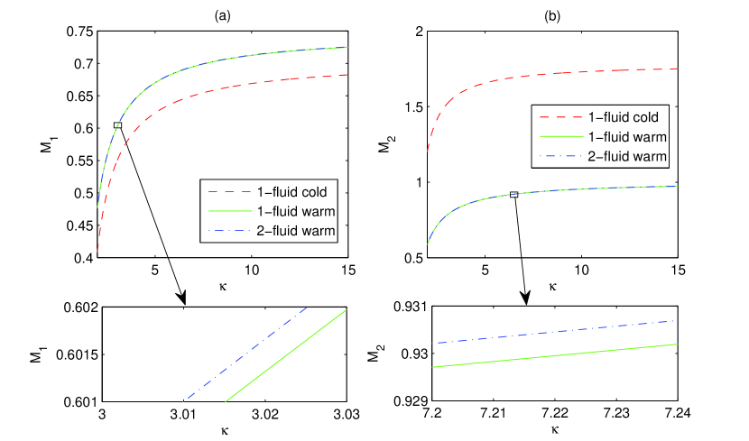
Figure 4.11: Variation of the lower limit $M_{1}$ and the upper limit $M_{2}$ with $\kappa$ for 1-fluid cold model (dashed curve), 1-fluid warm model (solid), and 2-fluid warm model (dot-dashed). As zoom-in shows difference between 1-fluid warm model and 2-fluid warm model are extremely small. Here, $\beta=2$, $\sigma=0.02$, $Z=1$, and $\mu=1/1836$.

We obtain the higher limit for the Mach number through $F_{2}(M,\beta,\kappa,{\sigma},\mu)=\Psi_{3}(\phi,M,\beta,\kappa,{\sigma},\mu)|_{\phi=\phi_{\max}^{(-)}}>0$, where $\phi_{\max}^{(-)}=-\frac{1}{2}\left({M-}\sqrt{3{\sigma}}\right)^{2}$. This gives:

$$F_{2}^{(-)}(M,\beta,\kappa,{\sigma},\mu) =(1+\beta)\frac{{M}^{2}}{{\mu}}\left(1-\left({1+\mu}+\frac{{\mu(3{\sigma}-2M}\sqrt{3{\sigma}})}{{M}^{2}}\right)^{1/2}\right)$$

$$+\beta\left(1-\left(1+\frac{\left({M-}\sqrt{3{\sigma}}\right)^{2}}{2\kappa-3}\right)^{-\kappa+3/2}\right)+M^{2}+\sigma-\frac{4M\sqrt{M\sqrt{3{\sigma}}}}{3}.$$ (4.25)

Hence, the upper limit $M_{2}^{(-)}(\beta,\kappa,{\sigma},\mu)$ is obtained by solving the above equation.

4.3.1 Ion Inertia Effects on Negative Soliton

Figure 4.11 shows that the ion inertia effects have trivially negative soliton existence altered. We notice that there is a extremely small difference between one-fluid warm model and two-fluid warm model. At the supersonic domain, positively charged heavy species behave like uniformly distributed positive background with negligible role in the dynamics of EAWs.

4.4 Positive Electron-Acoustic Soliton Existence

However, Eq. (4.23) has another solution, which yields the lower Mach number limit for positive solitary structures:

$$M_{1}^{(+)}(\beta,\kappa,{\sigma},\mu) =\frac{1}{2}\left(\frac{(\kappa-\tfrac{3}{2})\left[{\mu}(1+\beta)+1\right]}{\beta(\kappa-\frac{1}{2})}+3\sigma+2\left(\frac{3\sigma{\mu}(1+\beta)(\kappa-\tfrac{3}{2})}{\beta(\kappa-\frac{1}{2})}\right)^{1/2}\right)^{1/2}$$

$$-\frac{1}{2}\left(\frac{(\kappa-\tfrac{3}{2})\left[{\mu}(1+\beta)+1\right]}{\beta(\kappa-\frac{1}{2})}+3\sigma-2\left(\frac{3\sigma{\mu}(1+\beta)(\kappa-\tfrac{3}{2})}{\beta(\kappa-\frac{1}{2})}\right)^{1/2}\right)^{1/2}.$$ (4.26)

It is interesting to see that $\lim_{\mu\rightarrow 0}M_{1}^{(+)}(\beta,\kappa,{\sigma},\mu)=0$. This means that the one-fluid model involving inertial (cold or cool) electrons and inertialess ions may not produce positive solitons due to the dynamics of positively charged species being negligible.

We also derive the upper Mach number limit from $F_{2}(M,\beta,\kappa,{\sigma},\mu)$ = $\Psi_{3}(\phi,$ $M,\beta,\kappa,{\sigma},\mu)|_{\phi=\phi_{\max}^{(+)}}>0$, where $\phi_{\max}^{(+)}=\frac{1}{{2}}{\mu}^{-1}{{M}^{2}}$. This yields the following equation:

$$F_{2}^{(+)}(M,\beta,\kappa,{\sigma},\mu) =(1+\beta)\frac{{M}^{2}}{{\mu}}+\beta\left(1-\left(1-\frac{{{M}^{2}}}{{2\mu}\left(\kappa-\tfrac{3}{2}\right)}\right)^{-\kappa+3/2}\right)$$

$$+\frac{1}{6\sqrt{3{\sigma}}}\left(\left({M+}\sqrt{3{\sigma}}\right)^{3}+{{\left({M-}\sqrt{3{\sigma}}\right)^{3}}}\right.$$

$$\left.-\left[{\frac{1}{{\mu}}{{M}^{2}}+}\left({M+}\sqrt{3{\sigma}}\right)^{2}\right]^{3/2}-{\left[{\frac{1}{{\mu}}{{M}^{2}}+\left({M-}\sqrt{3{\sigma}}\right)^{2}}\right]}^{3/2}\right).$$ (4.27)

In the limit $\mu\rightarrow 0$, we find no solution to Eq. (4.27). This confirms our previous statement that the one-fluid model described in §2 and §3 cannot produce positive solitary waves.

4.4.1 Hot Electron Effects on Positive Soliton

Fig. 4.12 shows that $M_{1}$ and $M_{2}$ rise with the increase in the parameter $\beta$, i.e., the density of the hot electrons. This result is in contrast to the negative potential solitary wave (see Fig. 3.9). The existence domain for the positive potential solitary widens, as the hot electrons density is increased.

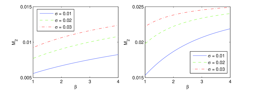
Figure 4.12: Positive potential soliton existence domain in the parameter space of $\beta$ and Mach number $M$ for different temperature ratio $\sigma$. (a) Variation of the lower limit $M_{1}$, (b) Variation of the upper limit $M_{2}$. Curves from bottom to top: $\sigma=0.01$ (solid), $\sigma=0.02$ (dashed), $0.03$ (dot-dashed curve). Here, $\kappa=3$, $Z=1$, and $\mu=1/1836$.

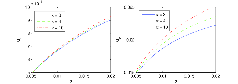
Figure 4.13: Positive potential soliton existence domain in the parameter space of $\sigma$ and Mach number $M$. Solitons may be supported in the region between $M_{1}(\sigma)$ and $M_{2}(\sigma)$. (a) Variation of $M_{1}(\sigma)$, (b) Variation of $M_{2}(\sigma)$. Curves from bottom to top: $\kappa=3$ (solid), $4$ (dashed), $10$ (dot-dashed curve). Here, Here, $\beta=2$, $Z=1$, and $\mu=1/1836$.

4.4.2 Temperature Effects on Positive Soliton

We also see that the two-fluid cold model ($\sigma\rightarrow 0$) may not propagate the positive solitary pulse, since $\lim_{\sigma\rightarrow 0}M_{1}^{(+)}(\beta,\kappa,{\sigma},\mu)=0$. Numerically solving Eq. (4.27) shows that the upper Mach number limit approaches zero in the limit $\sigma\rightarrow 0$. As illustrated in Fig. 4.13, the existence domain becomes narrower as the thermal velocity is decreased. This make difficult to find positive solitons at very low $\sigma$. In this figure, we see that moving into the Maxwellian distribution ($\kappa\rightarrow\infty$) will increase $M_{1}$ and $M_{2}$.

5 Conclusions

In this research, we have investigated linear and nonlinear EAWs in a suprathermal plasma consisting of cool (or cold) electrons, in the presence of hot suprathermal electrons and mobile (or motionless) ions. We began with the one-fluid cold ($T_{c}=0$) model, and advanced toward the one-fluid warm ($T_{c}\neq 0$) in the next step. Including mobile ions, we then approached the two-fluid warm model. Using small deviations from the equilibrium state to first order, we have obtained the linear dispersion relation for all three models. We use a Sagdeev pseudopotential method to investigate nonlinear structures of the electrostatic solitary waves. Our linear analysis has shown the weakly damped region for the EAWs, where waves can propagate, under the influence of hot suprathermal electron, thermal pressure, and ion inertia effects. Using nonlinear method, we determine the propagation speed and the existence of stationary profile solitary waves.

In the linear analysis, we found out that growing the suprathermal distribution, the hot electron number density and temperature, i.e., decreasing $\kappa$, increasing $\beta=n_{h,0}/n_{c,0}$, and decreasing $\sigma=T_{c}/T_{h}$, stretch the weakly damped region. We saw that the temperature effects dramatically change the dispersion relation. But, the ion inertia effect is trivial.

We can see that the absolute maximum electrostatic potential increases with the rise in the suprathermal distribution (decreasing $\kappa$), the hot electron number density, the hot electron temperature (decreasing $\sigma$). Nonetheless, the mobile ions have no essential role in the dynamics of supersonic negative solitary waves. The thermal velocity classifies the Mach number under two regions, namely supersonic ($M>\sqrt{3\sigma}$) and subsonic ($M<\sqrt{3\sigma}$) ranges. It is interesting to see that the ion-fluid supports positive subsonic acoustic-solitary waves, while the cool electron-fluid provides the negative supersonic solitons.

Finally, the nonlinear pseudopotential technique permits existence ranges for acoustic-solitary waves. The existence domain for the negative potential soliton becomes narrower with the increase in the suprathermal distribution, the hot electron number density, and the temperature ratio $\sigma$. The ion-fluid does not affect the negative soliton existence, but is necessary to maintain the positive solitary wave structure. The results showed that the positive acoustic-waves deeply depends on the suprathermal hot electron parameters ($\kappa$, density, and temperature). We saw that the two-fluid cold model ($T_{c}=0$) cannot predict the positive solitary pulses. The existence domain for the positive potential solitary becomes wider, as the hot electron number density and the temperature ratio $\sigma$ are increased, in contrast to the results for the negative solitary pulse.

To summarize, Chapter 2 showed how the hot suprathermal electrons have an effect on the weakly damped region and the propagation velocity range of the EAWs. The bipolar electric field structures rise as the hot electron number density is increased. Nonetheless, increasing the hot electron number density narrows the propagation velocity range. In Chapter 3, we saw how growing the cool temperature increases the damped region, and decreases the bipolar electric field amplitudes and the soliton existence. In Chapter 4, we studied the ion inertia effects on the EAWs, which does not affect much the negative solitary structures, but providing positive solitons on the slow scale. We also notice the positive acoustic solitary waves cannot be propagated in the two-fluid cold model.

To conclude, the electron temperature affects both negative and positive solitary wave structures. It was found that the mobile ion component has a trivial role in the supersonic (fast) region, but it appear to be very important in the subsonic (slow) region, leading to a novel acoustic wave. In the linear methodology, the ion inertia effect is also negligible. The ion temperature can be fully included to investigate any different possibilities (see Appendix B), but it is beyond the scope of this work.

Appendix A Analytical Basis

The project is composed of three steps (Models 1, 2, and 3):

$$\begin{array}[c]{ccc}\text{{\small Model 1 (Chapter \ref{singlecold}):}}&\left\{\begin{array}[c]{c}\tfrac{\partial n}{\partial t}+\tfrac{\partial(nu)}{\partial x}=0,\\ \\ \tfrac{\partial u}{\partial t}+\tfrac{u\partial u}{\partial x}=\tfrac{\partial\phi}{\partial x}\underset{\text{{\small Chapter \ref{warmmodel}; Eq. (\ref{eq2_9})} }}{\underbrace{-\tfrac{\sigma}{n}\tfrac{\partial P}{\partial x}}},\end{array}\right.&\begin{array}[c]{c}\text{{\small cool inertial electron continuity }}\\ \text{{\small and momentum equations; }}\\ \text{{\small Eqs. (\ref{eq1_10}) and (\ref{eq1_11})}}\end{array}\\ &&\\ \text{{\small Model 2 (Chapter \ref{warmmodel}):}}&\tfrac{\partial P}{\partial t}+\tfrac{u\partial P}{\partial x}+\tfrac{\gamma P\partial u}{\partial x}=0,&\begin{array}[c]{c}\text{{\small thermal pressure of cool inertial electron; }}\\ \text{{\small Eqs. (\ref{eq2_9}) and (\ref{eq2_10})}}\end{array}\\ &&\\ \text{{\small Model 3 (Chapter \ref{twofluidmodel}):}}&\left\{\begin{array}[c]{c}\tfrac{\partial\tilde{n}}{\partial t}+\tfrac{\partial(\tilde{n}\tilde{u})}{\partial x}=0,\\ \\ \tfrac{\partial\tilde{u}}{\partial t}+\tfrac{\tilde{u}\partial\tilde{u}}{\partial x}=-\tfrac{\mu\partial\phi}{\partial x},\end{array}\right.&\begin{array}[c]{c}\text{{\small ion inertial continuity }}\\ \text{{\small and momentum equations; }}\\ \text{{\small Eqs. (\ref{eq3_12}) and (\ref{eq3_13})}}\end{array}\end{array}$$

$$\begin{array}[c]{cc}\dfrac{\partial^{2}\phi}{\partial x^{2}}=\left\{\begin{array}[c]{cc}-(1+\beta)&\begin{array}[c]{c}\text{{\small inertialess ions}}\\ \text{{\small Chapters \ref{singlecold} and \ref{warmmodel}}}\end{array}\\ -\tilde{n}&\begin{array}[c]{c}\text{{\small inertial ions}}\\ \text{{\small Chapter \ref{twofluidmodel}}}\end{array}\end{array}\right.+\underset{\text{{\small Chapters \ref{singlecold},\ref{warmmodel}, and \ref{twofluidmodel}}}}{\underbrace{\underset{\begin{array}[c]{c}\text{{\small cool }}\\ \text{{\small electrons}}\end{array}}{\underbrace{n}}+\underset{\text{{\small hot suprathermal electrons}}}{\underbrace{\beta\left(1-\dfrac{\phi}{(\kappa-\tfrac{3}{2})}\right)^{-\kappa+1/2}}}},}&\begin{array}[c]{c}\text{{\small Poisson's equation}}\\ \text{{\small Eqs. (\ref{eq1_12}), (\ref{eq2_29}), and (\ref{eq3_14})}}\end{array}\end{array}$$

Appendix B An Alternative to Two-Fluid Model: Ion Temperature Effects

We may also consider the ion thermal pressure. Due to the thermal pressure of the ions, the equation of momentum contains an extra term (compare to Eq. (4.2))

$$\frac{\partial u_{i}}{\partial t}+u_{i}\frac{\partial u_{i}}{\partial x}=-\frac{Ze}{m_{i}}\frac{\partial\phi}{\partial x}-\frac{1}{m_{i}n_{i}}\frac{\partial P_{i}}{\partial x},$$ (B.1)

The pressure of the ions is given by

$$\frac{\partial P_{i}}{\partial t}+u_{i}\frac{\partial P_{i}}{\partial x}+\gamma P_{i}\frac{\partial u_{i}}{\partial x}=0,$$ (B.2)

where $P_{i}$ is the thermal pressure of the ions, in the one-dimensional model $\gamma=3$. We define the temperature ratio of the ions to the hot electrons as $\tilde{\sigma}=T_{i}/T_{h}$.

The normalized forms of Eqs. (B.1)–(B.2) are written as ($Z=1$ and $\gamma=3$):

$$\frac{\partial\tilde{u}}{\partial t}+\tilde{u}\frac{\partial\tilde{u}}{\partial x}=-\mu\frac{\partial\phi}{\partial x}-\frac{\mu\tilde{\sigma}}{\tilde{n}}\frac{\partial\tilde{P}}{\partial x}$$ (B.3)

$$\frac{\partial\tilde{P}}{\partial t}+\tilde{u}\frac{\partial\tilde{P}}{\partial x}+3\tilde{P}\frac{\partial\tilde{u}}{\partial x}=0,$$ (B.4)

The density $n_{i}$ are normalized with the unperturbed cool density ($n_{c,0}$), the velocity $u_{i}$ with the hot electron thermal velocity ($c_{h,s}=\left(k_{B}T_{h}/m_{e}\right)^{1/2}$), time with the inverse cool electron plasma frequency, $\omega_{pc}^{-1}$, where $\omega_{pc}=(n_{c,0}e^{2}/\varepsilon_{0}m_{e})^{1/2}$, length with the characteristic length scale, $\lambda_{0}=(\varepsilon_{0}k_{B}T_{h}/n_{c,0}e^{2})^{1/2}$, the wave potential $\phi$ with $k_{B}T_{h}/e$, and the pressure $P_{i}$ with $n_{c,0}k_{B}T_{i}$.

Integrating Eqs. (B.3) and (B.4) yield

$$\begin{array}[c]{cc}\tilde{u}=M{-}\sqrt{{M}^{2}{-2\mu\phi-3\mu\tilde{\sigma}\left[\tilde{n}^{2}-(1+\beta)^{2}\right]}},&\text{ \ }\tilde{P}=\tilde{n}^{3}.\end{array}$$ (B.5)

Combining Eqs. (4.16a)–(B.5), we get

$${\tilde{n}=}\frac{1}{2}\sqrt{\frac{\left({M+{(1+\beta)}}\sqrt{{{3\mu\tilde{\sigma}}}}\right)^{2}{-2\mu\phi}}{3{{\mu\tilde{\sigma}}}}}\pm\frac{1}{2}\sqrt{\frac{\left({M-{(1+\beta)}}\sqrt{{{3\mu\tilde{\sigma}}}}\right)^{2}{-2\mu\phi}}{3{{\mu\tilde{\sigma}}}}}$$ (B.6)

Therefore, the Sagdeev pseudopotential (4.21) is rewritten as

$$\Psi_{4}(\phi,M,\beta,\kappa,{\sigma},\tilde{\sigma},\mu)=-\beta\left(\left(1+\frac{\phi}{-\kappa+\tfrac{3}{2}}\right)^{-\kappa+3/2}-1\right)+M^{2}+\sigma$$

$$-\frac{1}{6\sqrt{3\sigma}}\left[{2\phi+}\left({M+\sqrt{3{\sigma}}}\right)^{2}\right]^{3/2}\mp\frac{1}{6\sqrt{3\sigma}}{\left[{2\phi+\left({M-\sqrt{3{\sigma}}}\right)^{2}}\right]}^{3/2}$$

$$+\frac{(1+\beta)}{{\mu}}\left[M^{2}+{(1+\beta)}^{2}\mu\sigma\right]-\frac{1}{6{\mu}\sqrt{3{{\mu\tilde{\sigma}}}}}\left[\left({M+{(1+\beta)}}\sqrt{{{3\mu\tilde{\sigma}}}}\right)^{2}{-2\mu\phi}\right]^{3/2}$$

$$\mp\frac{1}{6{\mu}\sqrt{3{{\mu\tilde{\sigma}}}}}\left[\left({M-{(1+\beta)}}\sqrt{{{3\mu\tilde{\sigma}}}}\right)^{2}{-2\mu\phi}\right]^{3/2}$$ (B.7)

In the limit $\tilde{\sigma}\rightarrow 0$, we get Eq. (4.21).

For the existence of acoustic-solitary waves moving at velocity $M$, we require $\Psi_{4}^{\prime}(\phi,M,\beta,\kappa,{\sigma},\tilde{\sigma},\mu)|_{\phi=0}=0$ and $F_{1}(M,\beta,\kappa,{\sigma},\tilde{\sigma},\mu)\equiv-\Psi_{4}^{\prime\prime}(\phi,M,\beta,\kappa,{\sigma},\tilde{\sigma},\mu)$ $|_{\phi=0}>0$. Here, the function $F_{1}(M)$ reads as

$$F_{1}(M,\beta,\kappa,{\sigma},\tilde{\sigma},\mu)=\frac{\beta(\kappa-\frac{1}{2})}{\kappa-\tfrac{3}{2}}-\frac{1}{M^{2}-3\sigma}-\frac{{(1+\beta)}\mu}{{M}^{2}{-{(1+\beta)}}^{2}{{3\mu\tilde{\sigma}}}},$$ (B.8)

where ${{(1+\beta)}}\sqrt{{{3\mu\tilde{\sigma}}}}$ is the normalized ion thermal velocity.

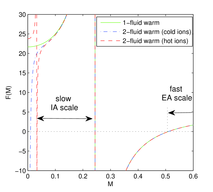
Figure B.1: The existence domains for stationary solitary structures. The quantities $F_{1}$ for 1-fuild warm model (solid), 2-fluid warm model for $T_{i}=0$ (dot-dashed), and 2-fluid cold model for $T_{i}\neq 0$ (dashed curve), are defined in (3.26), (4.23), and (B.8) respectively. Here, $\kappa=3$, $\beta=3$, $\sigma=0.02$, $\tilde{\sigma}=0.04$, $Z=1$, and $\mu=1/1836$.

We see that Eq. (B.8) contains an extra term corresponding to the ion thermal pressure (compare to Eq. (4.23)). The ion thermal velocity classifies the Mach number under two regions, namely “cool ion” (${M>{(1+\beta)}}\sqrt{{{3\mu\tilde{\sigma}}}}$) and “hot ion” (${M<{(1+\beta)}}\sqrt{{{3\mu\tilde{\sigma}}}}$), in the sense that the thermal velocity is smaller/larger than $M$, respectively. As illustrated in Fig. B.1, including the hot ion component ($T_{i}\neq 0$) divides the propagation speed into three ranges. Nonetheless, there are two existence ranges for solitary waves as Chapter 4. The existence range for positive acoustic-solitary waves has been effectively changed.

Appendix C Solving Biquadratic Equation

The quartic equation takes the form as

$$Q(x)=a_{4}x^{4}+a_{3}x^{3}+a_{2}x^{2}+a_{1}x+a_{0}.$$ (C.1)

If $a_{3}=a_{1}=0$, then we get the biquadratic equation

$$Q(x)=a_{4}x^{4}+a_{2}x^{2}+a_{0}.$$ (C.2)

Let assume $x=\sqrt{x_{1}}\pm\sqrt{x_{2}}$, we get $x^{2}=x_{1}+x_{2}\pm 2\sqrt{x_{1}x_{2}}$, and

$$\begin{array}[c]{cc}x_{1}+x_{2}=-\dfrac{a_{2}}{2a_{4}},&\text{ \ }x_{1}-x_{2}=\sqrt{\dfrac{a_{0}}{a_{4}}}.\end{array}$$ (C.3)

We then find the following solution to the biquadratic equation (C.2):

$$x=\sqrt{-\dfrac{a_{2}}{4a_{4}}+\dfrac{1}{2}\sqrt{\dfrac{a_{0}}{a_{4}}}}\pm\sqrt{-\dfrac{a_{2}}{4a_{4}}-\dfrac{1}{2}\sqrt{\dfrac{a_{0}}{a_{4}}}}.$$ (C.4)

References

- [1] M. Berthomier, R. Pottelette, and R. A. Treumann. Parametric study of kinetic Alfvén solitons in a two electron temperature plasma. Physics of Plasmas, 6:467–475, February 1999.
- [2] S. P. Gary and R. L. Tokar. The electron-acoustic mode. Physics of Fluids, 28:2439–2441, August 1985.
- [3] R. L. Tokar and S. P. Gary. Electrostatic hiss and the beam driven electron acoustic instability in the dayside polar cusp. Geophysical Research Letters, 11:1180–1183, December 1984.
- [4] H. Derfler and T. C. Simonen. Higher-Order Landau Modes. Physics of Fluids, 12:269–278, February 1969.
- [5] D. Henry and J. P. Treguier. Propagation of electronic longitudinal modes in a non-Maxwellian plasma. Journal of Plasma Physics, 8:311, December 1972.
- [6] S. Ikezawa and Y. Nakamura. Observation of electron plasma waves in plasma of two-temperature electrons. Journal of the Physical Society of Japan, 50:962–967, March 1981.
- [7] M. F. Thomsen, S. P. Gary, W. C. Feldman, T. E. Cole, and H. C. Barr. Stability of electron distributions within the earth’s bow shock. Journal of Geophysical Research, 88:3035–3045, April 1983.
- [8] W. C. Feldman, R. C. Anderson, S. J. Bame, S. P. Gary, J. T. Gosling, D. J. McComas, M. F. Thomsen, G. Paschmann, and M. M. Hoppe. Electron velocity distributions near the earth’s bow shock. Journal of Geophysical Research, 88:96–110, January 1983.
- [9] S. D. Bale, P. J. Kellogg, D. E. Larsen, R. P. Lin, K. Goetz, and R. P. Lepping. Bipolar electrostatic structures in the shock transition region: Evidence of electron phase space holes. Geophysical Research Letters, 25:2929–2932, 1998.
- [10] C. S. Lin, J. L. Burch, S. D. Shawhan, and D. A. Gurnett. Correlation of auroral hiss and upward electron beams near the polar cusp. Journal of Geophysical Research, 89:925–935, February 1984.
- [11] H. Matsumoto, H. Kojima, T. Miyatake, Y. Omura, M. Okada, I. Nagano, and M. Tsutsui. Electrotastic Solitary Waves (ESW) in the magnetotail: BEN wave forms observed by GEOTAIL. Geophysical Research Letters, 21:2915–2918, December 1994.
- [12] J. R. Franz, P. M. Kintner, and J. S. Pickett. POLAR observations of coherent electric field structures. Geophysical Research Letters, 25:1277–1280, 1998.
- [13] C. A. Cattell, J. Dombeck, J. R. Wygant, M. K. Hudson, F. S. Mozer, M. A. Temerin, W. K. Peterson, C. A. Kletzing, C. T. Russell, and R. F. Pfaff. Comparisons of Polar satellite observations of solitary wave velocities in the plasma sheet boundary and the high altitude cusp to those in the auroral zone. Geophysical Research Letters, 26:425–428, 1999.
- [14] A. P. Kakad, S. V. Singh, R. V. Reddy, G. S. Lakhina, and S. G. Tagare. Electron acoustic solitary waves in the Earth’s magnetotail region. Advances in Space Research, 43:1945–1949, June 2009.
- [15] K. Nishihara and M. Tajiri. Rarefaction ion acoustic solitons in two-electron-temperature plasma. Journal of the Physical Society of Japan, 50:4047–4053, December 1981.
- [16] M. P. Leubner. On Jupiter’s whistler emission. Journal of Geophysical Research, 87:6335–6338, August 1982.
- [17] T. P. Armstrong, M. T. Paonessa, E. V. Bell, II, and S. M. Krimigis. Voyager observations of Saturnian ion and electron phase space densities. Journal of Geophysical Research, 88:8893–8904, November 1983.
- [18] M. Berthomier, R. Pottelette, and M. Malingre. Solitary waves and weak double layers in a two-electron temperature auroral plasma. Journal of Geophysical Research, 103:4261–4270, March 1998.
- [19] P. Schippers, M. Blanc, N. André, I. Dandouras, G. R. Lewis, L. K. Gilbert, A. M. Persoon, N. Krupp, D. A. Gurnett, A. J. Coates, S. M. Krimigis, D. T. Young, and M. K. Dougherty. Multi-instrument analysis of electron populations in Saturn’s magnetosphere. Journal of Geophysical Research (Space Physics), 113:7208, July 2008.
- [20] M. A. Hellberg, R. L. Mace, R. J. Armstrong, and G. Karlstad. Electron-acoustic waves in the laboratory: an experiment revisited. Journal of Plasma Physics, 64:433–443, November 2000.
- [21] T. K. Baluku and M. A. Hellberg. Dust acoustic solitons in plasmas with kappa-distributed electrons and/or ions. Physics of Plasmas, 15(12):123705, December 2008.
- [22] N. S. Saini, I. Kourakis, and M. A. Hellberg. Arbitrary amplitude ion-acoustic solitary excitations in the presence of excess superthermal electrons. Physics of Plasmas, 16(6):062903, June 2009.
- [23] V. M. Vasyliunas. A survey of low-energy electrons in the evening sector of the magnetosphere with OGO 1 and OGO 3. Journal of Geophysical Research, 73:2839–2884, May 1968.
- [24] S. P. Christon, D. G. Mitchell, D. J. Williams, L. A. Frank, C. Y. Huang, and T. E. Eastman. Energy spectra of plasma sheet ions and electrons from about 50 eV/e to about 1 MeV during plamsa temperature transitions. Journal of Geophysical Research, 93:2562–2572, April 1988.
- [25] R. L. Mace and M. A. Hellberg. A dispersion function for plasmas containing superthermal particles. Physics of Plasmas, 2:2098–2109, June 1995.
- [26] H. Abbasi and H. H. Pajouh. Influence of trapped electrons on ion-acoustic solitons in plasmas with superthermal electrons. Physics of Plasmas, 14(1):012307, January 2007.
- [27] V. Pierrard and J. Lemaire. Lorentzian ion exosphere model. Journal of Geophysical Research, 101:7923–7934, April 1996.
- [28] D. Summers and R. M. Thorne. The modified plasma dispersion function. Physics of Fluids B, 3:1835–1847, August 1991.
- [29] R. L. Mace, G. Amery, and M. A. Hellberg. The electron-acoustic mode in a plasma with hot suprathermal and cool Maxwellian electrons. Physics of Plasmas, 6:44–49, January 1999.
- [30] M. A. Hellberg and R. L. Mace. Generalized plasma dispersion function for a plasma with a kappa-Maxwellian velocity distribution. Physics of Plasmas, 9:1495–1504, May 2002.
- [31] N. Dubouloz, R. Pottelette, M. Malingre, and R. A. Treumann. Generation of broadband electrostatic noise by electron acoustic solitons. Geophysical Research Letters, 18:155–158, February 1991.
- [32] M. Berthomier, R. Pottelette, M. Malingre, and Y. Khotyaintsev. Electron-acoustic solitons in an electron-beam plasma system. Physics of Plasmas, 7:2987–2994, July 2000.
- [33] S. V. Singh and G. S. Lakhina. Electron acoustic solitary waves with non-thermal distribution of electrons. Nonlinear Processes in Geophysics, 11:275–279, April 2004.
- [34] I. Kourakis and P. K. Shukla. Electron-acoustic plasma waves: Oblique modulation and envelope solitons. Physical Review E, 69(3):036411, March 2004.
- [35] T. S. Gill, H. Kaur, and N. S. Saini. Small amplitude electron-acoustic solitary waves in a plasma with nonthermal electrons. Chaos Solitons and Fractals, 30:1020–1024, November 2006.
- [36] B. D. Fried and R. W. Gould. Longitudinal Ion Oscillations in a Hot Plasma. Physics of Fluids, 4:139–147, January 1961.
- [37] R. Z. Sagdeev. Cooperative Phenomena and Shock Waves in Collisionless Plasmas. Reviews of Plasma Physics, 4:23, 1966.
- [38] F. Verheest, T. Cattaert, G. S. Lakhina, and S. V. Singh. Gas-dynamic description of electrostatic solitons. Journal of Plasma Physics, 70:237–250, April 2004.
- [39] J. F. McKenzie, E. Dubinin, K. Sauer, and T. B. Doyle. The application of the constants of motion to nonlinear stationary waves in complex plasmas: a unified fluid dynamic viewpoint. Journal of Plasma Physics, 70:431–462, August 2004.
- [40] F. Verheest, M. A. Hellberg, and G. S. Lakhina. Necessary conditions for the generation of acoustic solitons in magnetospheric and space plasmas with hot ions. Astrophysics and Space Sciences Transactions, 3:15–20, September 2007.