On the reinterpretation of non-resonant searches for Higgs boson pairs

Abstract

The detection of production of a pair of Higgs bosons before the end of LHC operation would be a clear evidence of New Physics (NP). As searches for non-resonant production of Higgs pairs are being designed it is of particular importance to be able to conveniently present current experimental results in terms of limits on the most ’model-independent’ fashion possible. In this article we provide an analytic parametrization of the differential Higgs-pair production at the LHC in the effective field theory (EFT) extension of the SM. It results from a fit to the theory prediction for the $gg\to hh$ cross section at the 13 TeV at the LHC. Subsequently the resulting formula is used for a reweighing technique that allows to recast to recast exclusion bounds from ATLAS and CMS HH$\to\gamma\gamma\,b\bar{b}$ searches to any point of the considered EFT parameter space. We demonstrate with a fast simulation of the LHC detectors that with this approach it is possible to cover the continuously of the EFT parameter space, taking correctly into account the efficiencies of signal selections, without the necessity of rerunning a large number of full detector simulations. Finally, the resulting exclusion bounds are confronted to several explicit models such as setups with additional scalars, including 2HDM, vector-like fermions, and minimal composite Higgs models, mapped to the EFT.

1 Introduction

Examining the production of pairs of Higgs bosons $h$ is a crucial task in the long term strategy of the LHC. Analysing this process offers a unique direct window on the Higgs potential, whose behaviour lies at the heart of many unresolved questions on nature, such as the hierarchy problem, the question of vacuum stability [1, 2, 3], the feasibility of electroweak baryogenesis [4, 5, 6], and the potential dynamical trigger for electroweak symmetry breaking (EWSB) [7, 8, 9] - just to name a few. Of particular importance regarding the search for physics beyond the Standard Model (SM) are differential observables, such as the distribution of the invariant mass of the Higgs pairs $m_{hh}$ (see, e.g., [10, 11, 12]), since they are especially sensitive to effects of new physics (NP).

As we eventually want to confront corresponding experimental results with theory, we need to assume a theoretical framework, which in our case will be the effective field theory (EFT) extension of the SM, supplementing it with higher dimensional operators. This captures the effects of any yet undiscovered physics beyond the SM, given that it is separated from the latter by a mass gap and in particular is significantly heavier than the scales probed experimentally. In that sense, the setup is ‘model independent’, providing the most general parametrization of nature, based on what we observe at low energies. On the other hand, any known UV model (residing at scales well beyond the electroweak scale) can be mapped to such an effective Lagrangian, rendering a formulation of experimental results in terms of bounds on its parameters an extremely useful bridge between data and theory. Having at hand analytic formulae which translate between observables in a realistic collider environment and effective couplings will thus be of utmost importance for the experimental results to be properly interpreted.

In this paper we will present on the one hand such a fit of the theory prediction for the Higgs-pair production cross section in gluon fusion at the LHC in terms of effective couplings, considering both the total cross section as well as the ones differential in $m_{hh}$ and $|cos\,\theta^{*}|$. At Leading Order (LO) the totality of the HH process is described by those two variables. Beyond that, we will employ the formula to reinterpret exclusion bounds, derived assuming certain benchmark points in parameter space with a given kinematics, for points with modified kinematic distributions. In fact, different distributions in variables, such as $m_{hh}$, will lead to different efficiencies of selection cuts, which can be accounted for, knowing the distributions in terms of effective couplings. Without such an analytic knowledge, a full monte-carlo (MC) simulation would actually be required for each parameter-space point, which is not feasible for a dense scan of the parameters. Finally, we will use the interpreted results to confront explicit models, mapped to an effective Lagrangian, efficiently with constraints from the LHC. To perform this exercise we collect from literature setups with additional scalars, including two-Higgs-doublet models (2HDM), vector-like fermions, and minimal composite Higgs models and provide a collection of relations between their explicit parameters and effective couplings after EWSB.

2 Setup

The theory, on which our analysis is based, is the EFT extension of the SM with $D=6$ operators ${\cal O}_{i}$ with coefficients $\sim c_{i}$, suppressed by the NP scale $\Lambda^{2}$ (assuming for the moment a linearly realized SM gauge symmetry). The terms relevant for the production of Higgs pairs in gluon fusion to leading order (LO) are contained in the effective Lagrangian [12]

$$\begin{split}{\cal L}={\cal L}_{\rm SM}&+\frac{c_{H}}{2\Lambda^{2}}(\partial^{\mu}|H|^{2})^{2}-\frac{c_{6}}{\Lambda^{2}}\lambda_{SM}|H|^{6}\\ &-\left(\frac{c_{t}}{\Lambda^{2}}y_{t}|H|^{2}\bar{Q}_{L}H^{c}t_{R}+\text{h.c.}\right)\\ &+\frac{\alpha_{s}c_{g}}{4\pi\Lambda^{2}}|H|^{2}G_{\mu\nu}^{a}G^{\mu\nu}_{a}\,.\end{split}$$ (1)

Here, ${\cal L}_{\rm SM}$ is the SM Lagrangian, $\lambda_{SM}=m_{h}^{2}/2v$ is the SM value of the tri-linear Higgs self coupling, with $m_{h}\approx 125$ GeV the mass of the Higgs boson, $y_{t}$ is the top-quark Yukawa coupling, and $\alpha_{s}$ is the strong coupling constant.

After EWSB (in unitary gauge) $H\to 1/\sqrt{2}\,(0,v+h)^{T}$, where $v/\sqrt{2}\equiv\langle|H|\rangle\approx 174$ GeV is the vacuum expectation value of the Higgs field, the terms relevant for the $gg\to hh$ process become [12, 11, 10]

$$\begin{split}{\cal L}_{h}=\frac{1}{2}\partial_{\mu}\,h\partial^{\mu}h-\frac{1}{2}m_{h}^{2}h^{2}-{\kappa_{\lambda}}\,\lambda_{SM}v\,h^{3}-\frac{m_{t}}{v}(v+{\kappa_{t}}\,h+\frac{c_{2}}{v}\,h\,h)\,(\bar{t}_{L}t_{R}+h.c.)\\ +\frac{1}{4}\frac{\alpha_{s}}{3\pi v}(c_{g}\,h-\frac{c_{2g}}{2v}\,h\,h)\,G^{\mu\nu}G_{\mu\nu}\,.\end{split}$$ (2)

In fact, the operators in (1) modify the trilinear Higgs self coupling and the top yukawa coupling, parametrized via multiplicative factors $\kappa_{\lambda}$ and $\kappa_{t}$, where in the SM $\kappa_{\lambda}=\kappa_{t}=1$. Beyond that, they induce additional contact interactions between two Higgs bosons and two fermions and between a gluon pair and one or two Higgs bosons, parametrized by $c_{2},c_{g},$ and $c_{2g}$, which vanish in the SM, i.e., $c_{2}=c_{g}=c_{2g}=0$. The relations between these effective couplings and the coefficients of the operators in Eq. (1) can be obtained straightforwardly (see, e.g., [12]) and imply the constraint $c_{g}=-c_{2g}$. This correlation is however broken in the non-linear realization of EWSB and is not assumed a priori in this work, where we treat all couplings in Eq. (2) as free. In the next section, we will provide a parametrization of the Higgs-pair production cross sections in terms of the effective couplings entering the effective Lagrangian (2).

3 Fit to the (differential) $gg\to hh$ cross section

We will now describe our fit to the cross section for Higgs pair production in gluon fusion at the 13 TeV LHC in the EFT defined above. We consider the total cross section but as well as the ones differential in $m_{hh}$ and $|cos\,\theta^{*}|$, with $\theta^{*}$ being the polar angle of either of the Higgs bosons with respect to the beam axis (featuring the same $|cos\,\theta^{*}|$ at parton level).

Examining the different contributions to the full amplitude, it is easy to see that the $gg\to hh$ cross section $\sigma_{hh}\equiv\sigma(gg\to hh)$ (normalized to its SM value $\sigma_{hh}^{SM}$) can be parametrized to LO in terms of the parameters in (2) as [10]

$$\begin{split}R_{hh}\equiv\frac{\sigma_{hh}}{\sigma_{hh}^{SM}}={\rm Poly}(\mathbf{A})=\ &A_{1}\,\kappa_{t}^{4}+A_{2}\,c_{2}^{2}+(A_{3}\,\kappa_{t}^{2}+A_{4}\,c_{g}^{2})\,\kappa_{\lambda}^{2}+A_{5}\,c_{2g}^{2}+(A_{6}\,c_{2}+A_{7}\,\kappa_{t}\kappa_{\lambda})\kappa_{t}^{2}\\ &+(A_{8}\,\kappa_{t}\kappa_{\lambda}+A_{9}\,c_{g}\kappa_{\lambda})c_{2}+A_{10}\,c_{2}c_{2g}+(A_{11}\,c_{g}\kappa_{\lambda}+A_{12}\,c_{2g})\,\kappa_{t}^{2}\\ &+(A_{13}\,\kappa_{\lambda}c_{g}+A_{14}\,c_{2g})\,\kappa_{t}\kappa_{\lambda}+A_{15}\,c_{g}c_{2g}\kappa_{\lambda}\end{split}\,.$$ (3)

In Ref. [10], the parameters $A_{i}$, that form a vector $\mathbf{A}\equiv(A_{i})$ of coefficients of the polynomial ${\rm Poly}(\mathbf{A})$, were extracted from simulations to describe the total cross section. In this paper, we push the logic further to describe the differential cross section. We slice the kinematic space into bins with sufficient granularity. In each bin, Eq. 3 holds, but the coefficients become bin dependent, $A_{i}\to A_{i}^{j}$ , following the matrix-element (ME) integration and the PDF evolution. We define the cross section in a bin $j$ by $\sigma_{hh,j}\equiv\sigma_{hh}\times{\rm Frac}^{j}$, where ${\rm Frac}^{j}$ is the fraction of events contained in bin $j$. The differential $hh$ production ratio now becomes

$$R_{hh}^{j}\equiv\frac{\sigma_{hh}}{\sigma_{hh}^{\rm SM}}\frac{{\rm Frac}^{j}}{{\rm Frac}_{\rm SM}^{j}}={\rm Poly}(\mathbf{A}^{j})\,.$$ (4)

We simulate the differential cross section for various points in the five-dimensional parameter space, spanned by $\{\kappa_{\lambda},\kappa_{t},c_{2},c_{g},c_{2g}\}$, to determine $\mathbf{A}^{j}$. At LO accuracy the ME information differential in the invariant mass of the Higgs pair ($m_{hh}$) and in $|cos\,\theta^{*}|$ completely defines the 2$\to$2 process. At any subsequent simulation step - after the Higgs decays - the process evolution is independent of the NP at high energies, up to detector level. Therefore the results based on the ME-level information are applicable to reconstruct NP shapes at LO at detector level, provided that the former is known on an event-by-event basis.

After an optimization procedure, we converged to an optimal list of 59 bins in $m_{hh}$ that allowed for a precise reweighing of an ensemble of generated events to any NP shape. Since the distribution in the $cos\,\theta^{*}$ variable is rather flat, only 4 bins are considered. For the binning in $m_{hh}$ we choose 10 GeV intervals up to 700 GeV, where the bulk of the cross section is observed, and use a more coarse binning above. Explicitly, our binning is given by

$$m_{hh}$$ [GeV] = [250, 260, 270, 280, 290, 300, 310, 320, 330, 340,

 350, 360, 370, 380, 390, 400, 410, 420, 430, 440,

 450, 460, 470, 480, 490, 500, 510, 520, 530, 540,

 550, 560, 570, 580, 590, 600, 610, 620, 630, 640,

 650, 660, 670, 680, 690, 700,

 750, 800, 850, 900, 950, 1000, 1100, 1200, 1300, 1400,

 1500, 1750, 2000, 13000]

    = [0,0.4,0.6,0.8,1]   .

(5)

Following the procedure established in [10], the components of $\mathbf{A}^{j}$ are extracted by maximizing the likelihood simultaneously for all the coefficients, employing an ensemble of MC simulated samples, scanning the model parameters, i.e., minimizing

$$\log L(\mathbf{A}^{j})=-\sum_{i}\left(\frac{T^{(i,j)}-\sigma_{hh}^{i}(\mathbf{A}^{j})}{\delta T^{(i,j)}}\right)^{2}\,,$$ (6)

where the index $i$ runs over different points in the $\{\kappa_{\lambda},\kappa_{t},c_{2},c_{g},c_{2g}\}$ parameter space. Here, $T^{(i,j)}\equiv\sigma_{hh,MC}^{i}\,{\rm Frac}_{i}^{j}$, with $\sigma_{hh,MC}^{i}$ the total cross section calculated via MC simulation and ${\rm Frac}_{i}^{j}$ the corresponding bin fraction (also taken from MC), while $\sigma_{hh}^{i}(\mathbf{A}^{j})\equiv R_{hh}^{j}\,\sigma_{hh}^{\rm SM}\,{\rm Frac}_{\rm SM}^{j}$ is the differential cross section parametrization following Eq. 4. Only the statistical (MC) uncertainty on the cross section in each bin, $\delta T^{(i,j)}$, is considered. For the SM point we assume a non-zero value of $10^{-4}$ to regularize the likelihood.

A careful choice of NP parameters is considered in the simulation to improve the convergence of the procedure. In particular it is important to avoid negative $R_{hh}^{j}$ values due to statistical fluctuations and, in general, a very poor population of certain bins (due to the limited total statistics). We thus consider simulated datasets such that the minimization of equation 6 can be done in parameter-subspaces (S$k$) with lower dimensionality that nevertheless contain the full information and guarantee appropriate statistics for all bins. The list of subspaces and the coefficients that they serve to determine are compiled in Table 1.

The simulation of events is performed within the MG5_aMC@NLO framework [15] where the entire event generation process is automated [16]. We make use of UFO model files [17] extracted from the Lagrangian 1, as constructed by the authors of Ref. [18]. For each NP point we simulate 50,000 events, while for the SM benchmark we generate a sample of 13,000,000 events.

Subspace	Parameters	Coefficients to be determined	scan
S1	$\kappa_{\lambda},\,\kappa_{t}$	$A_{1}^{j},\,A_{3}^{j},\,A_{7}^{j}$	kl = E-4, +-2.5, +-5, +- 7.5, +- 10, +- 12.5, +- 15
			kt from 0.5 to 2.5 with steps of 0.5
S2	$\kappa_{\lambda},\,c_{2},\,c_{g},\,c_{2g}$	$A_{2}^{j},\,A_{5}^{j},\,A_{10}^{j},\,A_{15}^{j}$	c2 = +-1, +-3 , c2g = +-0.5, +-1.5
			kl = 1 +-5, +- 10 and (cg,c2g) = +-1 (independently)
S3	$\kappa_{\lambda},\,c_{2},\,c_{g}$	$A_{4}^{j},A_{9}^{j}$	kl = 1 +-5, +- 10 , cg = +-1 and c2 = +-1, +-3
S4	$\kappa_{\lambda},\,\kappa_{t},\,c_{2}$	$A_{6}^{j},\,A_{8}^{j}$	kl = 1 +-5, +- 10, kt from 0.5 to 2.5 with steps of 1.0 and c2 = +-1, +-3
S5	$\kappa_{\lambda},\,\kappa_{t},\,c_{2g},\,c_{g}$	$A_{12}^{j},\,A_{14}^{j}$	kl = 1 +-5, +- 10, kt from 0.5 to 2.5, (cg,c2g) = +-1 (independently)
Additional points to better precise some coefficients (fixing $\kappa_{\lambda}=\kappa_{t}=e^{-4}$)
$A_{2}^{j}$		c2 from -3 to 3 in steps of 0.5
$A_{10}^{j}$		c2 = +-1, +-3 and c2g = +-0.5, +-1.5
$A_{15}^{j}$		(cg , -c2g) = +-0.5, +-1.5 (independently)

Table 1: Definition of the lower dimensional subsets (S$k$) to find the coefficients of equation 4.

Our results for the fit coefficients are compiled in Tables 9-12. To illustrate the bin statistics, we also show the number of events in each bin, both for our total BSM sample (see Section 4) and the SM sample.

In Figure 1 we provide some examples of the fit agreement with the dataset points to selected $m_{hh}$ ranges considering the bin central in $cos\,\theta^{*}$. Here, we display three parameter space directions, which are $\kappa_{\lambda}$ for fixed $\kappa_{t}=1$, $\kappa_{t}$ for $\kappa_{\lambda}=10^{-4}$ and $c_{2}$ for $\kappa_{\lambda}=1$, $\kappa_{t}=1.5$. The errors on the data points are purely statistical, while the coloured lines correspond to the fit result, Eq. (4). It becomes evident from the results that, even if it is true that for every bin one needs only a minimum of $N_{\rm fit}=15$ different samples to determine all coefficients, due to limited MC statistics the result of such a procedure would have a limited reliability. Concerning the behaviour of the cross section in different bins, the results confirm the expectation that a change in the scalar self coupling $\kappa_{\lambda}$ affects mostly the threshold region, while the ($D>4$) $\bar{t}thh$ contact interaction has a large effect on the high energy tail. Moreover, the pronounced destructive interference present in the cross section in the vicinity of the SM point $\kappa_{\lambda}=1$ becomes evident via the peaked minimum, visible in the left-most plot.

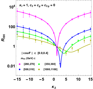
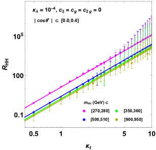
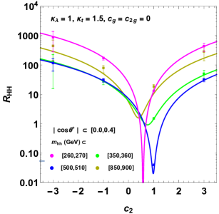
Figure 1: Comparison of $R_{hh}^{j}$, obtained from the analytical formula (4), with the same ratio, as derived directly via MC, for the most central bin in $\cos\theta^{\ast}$ (betweem 0 and 0.4) and for four different bins in $m_{hh}$, which are between 260 GeV and 270 GeV (threshold), 350 GeV and 360 GeV (interference region), 500 GeV and 510 GeV, and 1000 GeV and 1100 GeV (high mass tails). From left to right we show a scan in $k_{\lambda}$, $k_{t}$ and $c_{2}$, respectively, while keeping the other parameters at fixed values The error bars have a pure statistical source related with the generated number of events.

In Figure 2 we display the value of the coefficients of $R_{hh}^{j}$ for the central $\cos\theta^{\ast}$ bin as a function of $m_{hh}$, grouped in the subspaces given in Table 1. As a first observation, we see that at high invariant masses $A_{2,5,10}$ become most important, which coincide with the terms that parametrize genuine higher dimensional effects (containing exclusively $c_{2,g,2g}$), in agreement with expectations. We further note that for the subspace that corresponds solely to a variation of SM parameters (S1, with coefficients $A_{1,3,7}$), the absolute value of the coefficients does not surpass 100, and they are peaked towards low $m_{hh}$. In particular, the value of $A_{7}$ (that controls the triangle-box interference term $\sim\kappa_{t}^{2}\kappa_{t}\kappa_{\lambda}$) is always negative for $m_{hh}<400$ GeV. In subspace S2 (coefficients $A_{2,6,8}$), which features the contributions from the new $\bar{t}thh$ contact interaction (including interference with SM-like contributions), the coefficients are in general larger compared to those in S1, resulting in stronger variations with the corresponding parameters close to the $hh$ threshold, and show more pronounced $m_{hh}$ tails, as discussed before. Finally, all the remaining terms contain gluon-Higgs contact interactions and as such also feature pronounced contributions at large energies. The Feynman-diagrammatic representation of the different contributions to the cross section can be studied in Figure 1 of [10].

After this general discussion of the behavior of the cross section and the fit coefficients, in the next section we will employ Eq. (4) to reinterpret experimental analyses.

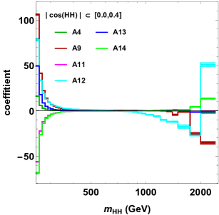
Figure 2: Values of the fit coefficients entering $R_{hh}^{j}$, differential in $m_{hh}$. We only display the results for the central $\cos\theta^{\ast}$ bin (betweem 0 and 0.4). From left to right, we show the coefficients belonging to subspaces (S1,S2), S4, and (S3, S5, S6), respectively (see Table 1).

4 Recast of ATLAS and CMS measurements

In this section we establish and validate the reweighting method and estimate the present limits on the Higgs couplings in a multi-dimensional space. The constraints are obtained by a recast of preliminary results from the ATLAS and CMS collaborations [19, 20] in the $HH\rightarrow\gamma\gamma b\bar{b}$ channel, that refer, respectively, to samples of 3.2 fb^-1 and 2.7 fb^-1 of 13 TeV data. Results with a slightly better sensitivity were published employing 8 TeV data [21, 22, 23], but we decided to use the preliminary results since they are obtained at the same center-of-mass energy that will be used for the next generation of LHC results. Between the publications of these and the release of this paper, other searches were performed by both collaboration in several channels [24, 25, 21] and with more luminosity, were the CMS analyses also include results for beyond the SM (BSM) scans in $\kappa_{\lambda}$ and $\kappa_{t}$.

The choice of the $HH\rightarrow\gamma\gamma b\bar{b}$ channel results from the fact that this final state is easy to simulate and to reconstruct using a parametric model of the ATLAS and CMS detectors. Moreover, both analyses were performed with a sequential application of selections (in contrast to a multivariate analysis that is a kind of standard now), making them easy to recast. It is known that this final state is less constrained in regions of the phase-space compared to other final states [21]. Nevertheless, since our goal is the proof of principle of the recast technique, we are not hunting for the latest and best limit. In the case of more sophisticated (multivariate) analyses, a reinterpretation of the results is more subtle, however still possible if samples exist for all relevant kinematic configurations, as provided in [10] (see discussion at the end of Section 5).

4.1 Signal simulation and reweighing

We employ Eq. 4 to reweight a set of base events to different points in the parameter space. As base events, we use the 12 benchmarks defined in [10, 26, 27] and for each of them we simulate 100,000 events. Due to the construction of the benchmarks, the resulting ensemble $\mathcal{S}_{\rm BSM}$ of 1,200,000 events populates well the EFT space we are probing. In addition 100,000 SM-like events are generated for comparison but kept out of $\mathcal{S}_{\rm BSM}$.

The hard scattering events are generated at LO accuracy using the model described in section 3. Following Ref. [26] we normalize the events to a total cross section with a k-factor is applied to include corrections up to NNLO (augmented with NNLL re-summation) in QCD ($\sigma_{hh}^{\rm SM}=33.5\pm 1.4$ fb  [27]). Note that the normalization only becomes relevant to predict the absolute number of events, as used in Section 5. In fact, up to NNLO, the k-factors are found to be mostly flat in kinematic variables as well as as a function of the EFT parameters (in the bulk of the parmeterspace) [28] and this suggests that the distributions are well described by performing the reweighing with LO information and employing flat k-factors to correct for QCD corrections at the end is a reasonable approximation. Furthermore, we used the NLO set of the PDF4LHC parton densities [29, 30, 31, 32] as well as the parton shower and hadronization infrastructure of the Pythia 8 package [33]. Finally, we simulate the response of an LHC-like detector by using Delphes 3  [34].

To reweight simulated events from $\mathcal{S}_{\rm BSM}$ to any other point in parameter space (such as the SM point, which we will use for validation), we apply an event-by-event weight

$$W_{i}=\frac{R_{hh}(m_{HH}^{i},cos\,\theta^{*}_{i})}{N_{i}}\cdot\frac{\sigma_{hh}^{\rm SM}\,{\rm Frac}_{\rm SM}^{j}}{\sigma_{hh}\ C_{\rm norm}}$$ (7)

where $m_{hh}^{i}$ and $cos\,\theta^{*}_{i}$ refer to the ME level variables corresponding to event $i$, and $N_{i}$ is the number of events in bin $j$ that contains $m_{hh}^{i}$ and $cos\,\theta^{*}_{i}$ in the reweighting sample $\mathcal{S}_{\rm BSM}$. Along the same lines, $R_{hh}(m_{HH}^{i},cos\,\theta^{*}_{i})$ is given by $R_{hh}^{j}$ (Eq. (4)) for this bin. It is our choice to normalize the weights in such a way that the resulting BSM distribution is normalized to one if no cut is applied and to the signal efficiency if any selection is applied. In this manner we decouple the shape information from the total cross section information.

The normalization coefficient $C_{\rm norm}$ is obtained as

$$C_{\rm norm}=\sum\limits_{j}R_{hh}^{j}\frac{\sigma_{hh}^{\rm SM}}{\sigma_{hh}}{\rm Frac}_{\rm SM}^{j}$$ (8)

and is used to unitarize the reweighed shape. In the ideal case $C_{\rm norm}=1$. Nevertheless, fluctuations in the samples used to derive the weights can induce a departure from unitarity. For the SM shape $C_{\rm norm}=1$, since the bin-by-bin fits are performed fixing the SM point and statistical errors occur only for BSM points where for some samples there are bins with inevitably low statistics (for example in the high $m_{HH}$ bins of threshold-like EFT points). After the renormalization procedure we observe a good agreement within the statistical uncertainties between MC simulation and reweighed samples, as can be seen in the next section.

4.2 The analyses

We consider the number of events $N_{\rm obs}$ observed by each experiment in a signal region and $B$ the number of the expected background events. In the ATLAS documents both values are directly provided in the text, while in the CMS document they are extracted from figures imposing a $M_{\gamma\gamma}$ window identical to the ATLAS one.

Both experiments found that the observed events are statistically compatibles with the expected SM backgrounds. Therefore, we can use this observation to derive exclusion limits on the maximal allowed number of (expected) events in a NP scenario $N_{\rm BSM}$ that could be compatible at 95% CL with the observed data. We build a Poissonian statistical likelihood

$$\mathcal{L}=e^{-(B+S)}\frac{(B+S)^{N_{\rm obs}}}{N_{\rm obs}!}\,,$$ (9)

where $S$ is the number of Signal events. Bayesian hypothesis with a uniform prior on $S$ allows to invert the likelihood to obtain a posterior as a function of $S$, normalized to unity between $S=[0,\infty]$. The likelihoods are shown in Figure 3. We integrate then the likelihood from 0 to 95% to obtain the 2 standard deviation confidence level value for $N_{\rm BSM}$. The number of observed, expected and excluded events are provided in Table 2. In this table we also include the number of events that would be excluded at $L$=100 fb^-1, projected assuming $N_{\rm obs}(\mbox{100 fb}^{-1})=B(\mbox{100 fb}^{-1})=L*B/L^{\prime}$, where $L^{\prime}$ is the data luminosity currently used.

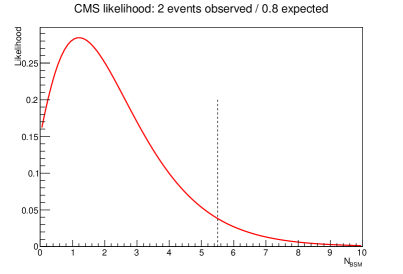
Figure 3: ATLAS and CMS likelihoods.

ATLAS				CMS
$N_{\rm obs}$	$B$	$N_{\rm BSM}$ (2.7 fb-1)	$N_{\rm BSM}$ (100 fb-1)	$N_{\rm obs}$	$B$	$N_{\rm BSM}$ (3.2 fb-1)	$N_{\rm BSM}$ (100 fb-1)
0	1.8	3.0	16.3	2	0.8	5.45	12

Table 2: Upper limits on cross section times luminosity in the analysis window, $N_{\rm BSM}$, from the recast of ATLAS and CMS results.

To translate the limit on $N_{\rm BSM}$ into the limit on the BSM cross section $\sigma_{\rm BSM}$ we need to know the selection efficiency $\epsilon$ within the signal box and the luminosity $L$: $\sigma_{\rm BSM}=N_{\rm BSM}/(L\epsilon)$. For both analyses we can extract (or estimate) $\epsilon_{\rm SM}$, i.e., the efficiency for the SM-like $hh$ production, from the information provided in the respective papers. What is not known a priori is the efficiency for a given BSM model with the associated choice of parameters. To estimate this, we employ a mock-up of the ATLAS and CMS analyses with Delphes 3 . The resulting efficiency $\epsilon_{D}$ is then rescaled (if needed) by a fudge factor $f_{\rm SM}=\epsilon_{\rm SM}/\epsilon_{\rm SM,D}$ to get an estimate of the real efficiency $\epsilon_{\rm BSM}\approx f_{\rm SM}\cdot\epsilon_{D}$. This factor takes into account the limited information we benefit from to emulate the analysis and the approximations made in Delphes 3  to describe the detector response, such as the efficiency of detecting photons or tagging b-jets. Note that this step could be avoided if the experimental collaborations would make public the full information (including the generation level $m_{hh}$ and $|cos\,\theta^{*}|$ variables) on the events that pass the signal selection.

In Table 3 we summarize the set of selections of both ATLAS and CMS searches. It is important to notice that the same Delphes 3 card was used for both experiments. This approximation is valid for photons in the energy range considered in $hh$ production since both experiments are more than 90% efficient to tag them. The difference in fiducial acceptance is emulated at the level of selections. For jets, both experiments use the anti-k_T algorithm [35] with radius parameter 0.4. Their acceptance and calibrations are similar at those energies. The major difference comes from the b-tagging working point (WP). Since both experiments require both jets to be b-tagged we just rescale the typical efficiency of the WP used in Delphes 3 within our $p_{T}$ and $\eta$ range (63% – see Ref. [36]) to the efficiency of the WP declared in the public notes, i.e., 85% for ATLAS and 78% for CMS. Finally, for the projections to $100\,$fb^-1 given below, we assume the observed number of events to match the expected and no improvements in the analysis, which is a very conservative assumption.

variable	ATLAS	CMS
$|\eta_{max}|$	2.37	2.5
Rejected fiducial region in $|\eta|$	[1.37, 1.52]	[1.44, 1.57]
Leading photon $(p_{T,min})$	—	30
Subleading photon $(p_{T,min})$	—	20
Leading photon $(p_{T,min})/M_{\gamma\gamma}$	0.35	1/3
Trailing photon $(p_{T,min})/M_{\gamma\gamma}$	1/4
$\Delta R$ with any jet	$>0.4$
$|\eta_{max,b}|$	2.5	2.4
Leading b-jet $p_{T,min}$ (GeV)	55	25
Trailing b-jet $p_{T,min}$ (GeV)	35	25
$M_{\gamma\gamma}$ window (GeV)	[122, 128]
$M_{b\bar{b}}$ window (GeV)	[95,135]	[80,200]
$M_{\gamma\gamma b\bar{b}}$ minimum (GeV)	—	350

Table 3: Selections used in the recast analyses.

After the reweighting according to the b-tagging properties and the selections of Table 3, we find the efficiencies shown in Table 4. It appears that for the ATLAS analysis our efficiencies have to be rescaled by $f_{\rm SM}=1.41$. Beside the usual suspects described above to explain the size of the factor, we suspect that the photon efficiency is slightly better in the real ATLAS analysis than in the Delphes 3 card, but the exact amount is hard to guess from the details given in the conference note.

In the CMS case the efficiency of the 2 b-tag and 1 b-tag categories are only provided together and no explicit information on how it is distributed between them is given. One may notice that a similar categorization was used at 8  TeV where the events appeared to be evenly split between the two categories, incidentally [23]. We apply the same assumption to the 13 TeV analysis and split the efficiencies evenly between the two categories ($\epsilon_{\rm SM,CMS}\approx 10\%$ per category).

ATLAS			CMS
$\epsilon_{\rm SM,D}$	$\epsilon_{\rm SM}$	$f_{\rm SM}$	$\epsilon_{\rm SM,D}$	$\epsilon_{\rm SM}$	$f_{\rm SM}$
7.1%	10%	1.41	10.8%	$\approx 10\%$	1

Table 4: Results from the ATLAS and CMS-like recast. See text for details.

4.3 Validation of the analytical reweighing

In Figure 4 we show the comparison of the actual simulation and the reweighting for an SM-like signal for 3 main reconstructed kinematic variables describing the hh system: $m_{X}\equiv m_{\gamma\gamma b\bar{b}}-m_{b\bar{b}}-m_{\gamma\gamma}+250\,{\rm GeV}$, cos $\theta^{*}_{\rm\gamma\gamma b\bar{b}}$ and $p_{\rm T,\gamma\gamma b\bar{b}}$. The first variable was shown to be the best estimate of $m_{hh}$ in Ref. [20]. The statistical errors per bin are shown only for the plain simulation, since the shapes derived by reweighting are constructed from 12 times as much bare events and thus expected to have less statistical fluctuations. In general we find a very good agreement between the distributions. Comparisons for different benchmarks provide similar picture and are given in Appendix B. Moreover, in Figure 5 we show reweighted distributions in $m_{X}$, after ATLAS-like selections, for BSM points not within the set of (simulated) benchmarks. Beyond points featuring non-vanishing contact interactions (cg=-c2g=1 and c2=1), we also consider the maximum box-triangle interference (kl=2.4), thereby exploring three different kinematic regimes. In all the cases we see smooth shapes.

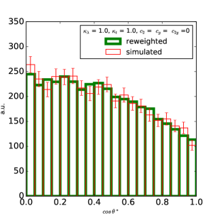
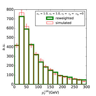
Figure 4: Reconstructed variables after ATLAS-like selection for the di-Higgs system. The histograms display the signal efficiency times 100,000 events.

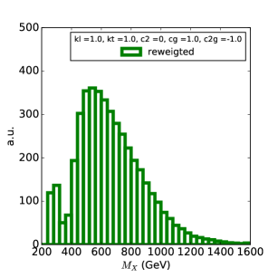
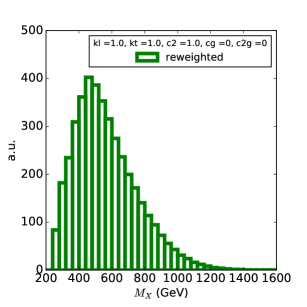
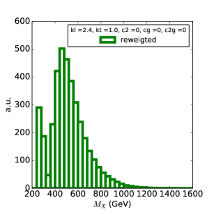
Figure 5: Reconstructed variables after ATLAS-like selection for the $m_{X}$ variable for three BSM points with different kinematic properties. The histograms display the signal efficiency times 100,000 events.

Finally, the efficiencies of different benchmark points obtained from the MC simulation are given in Table 5 ($\epsilon_{MC}$), together with the reweighted efficiencies as obtained after applying the renormalization via $C_{norm}$. The agreement of both efficiencies is remarkable, specially in the points where EFT is linear (where the parameter space scan used for the fit is more dense, see table 1).

							ATLAS-like		CMS-like
$N$	$\kappa_{\lambda}$	$\kappa_{t}$	$c_{2}$	$c_{g}$	$c_{2g}$	$C_{\rm norm}$	$\epsilon_{\rm MC}$	$\epsilon_{\rm rew}$	$\epsilon_{\rm MC}$	$\epsilon_{\rm rew}$
0	1.0	1.0	0.0	0.0	0.0	1.0	10.0	10.0	11.46	11.47
1	7.5	1.0	-1.0	0.0	0.0	0.94	10.6	10.6	10.83	10.79
2	1.0	1.0	0.5	-0.8	0.6	0.71	10.3	10.4	11.46	11.26
3	1.0	1.5	-1.5	0.0	-0.8	0.96	9.93	10.5	10.89	11.68
4	-3.5	1.0	-3.0	0.0	0.0	0.98	9.42	9.37	9.89	9.72
5	1.0	1.0	0.0	0.8	-1.0	0.88	11.6	11.5	12.47	12.50
6	2.4	1.0	0.0	0.2	-0.2	0.96	8.47	8.73	7.27	7.74
7	5.0	1.0	0.0	0.2	-0.2	1.01	6.24	6.17	3.30	3.23
8	15.0	1.0	0.0	-1.0	1.0	0.92	10.2	10.3	10.64	10.74
9	1.0	1.0	1.0	-0.6	0.6	0.86	11.6	11.6	12.92	12.79
10	10.0	1.5	-1.0	0.0	0.0	1.01	6.67	6.60	3.48	3.48
11	2.4	1.0	0.0	1.0	-1.0	0.95	8.16	8.26	6.72	6.81
12	15.0	1.0	1.0	0.0	0.0	1.0	7.80	7.52	6.23	6.17

Table 5: The renormalization factor ($C_{\rm norm}$) for benchmark point $N$ as well as MC and reweighted sample efficiencies.

5 Model dependent interpretations

We illustrate the method described in Section 4 reinterpreting EFT bounds, applying them to concrete NP setups. We consider the explicit models collected in Table 6.

Model	NP integrated out	Ref.
1	real scalar singlet with explicit $Z_{2}$ breaking	[37, 38]
2	real scalar singlet with spontaneous $Z_{2}$ breaking	[37]
3	real scalar triplet	[37, 38]
4	complex scalar triplet	[37, 38]
5	quartet scalar with $Y=1/2$	[37, 38]
6	quartet scalar with $Y=3/2$	[37, 38]
7	2HDM (addtl. scalars heavy + $Z_{2}$)	[39]
8	vector-like quark: $T$ (singlet top partner)	[40]
9	vector-like lepton: $E$ (flavor universal singlet)	[41]
10	MCHM5	[7, 42, 8, 43]
11	MCHM4	[7, 42, 8, 43]

Table 6: Explicit models considered in this work.

In Table 7 we provide the relations between the effective couplings for the various models under consideration, arising after integrating out the NP at tree level, where we express dependent couplings in terms of independent ones, the latter given in the second column. The relation with the fundamental parameters of the models is given in Table 8, which contains equivalent information. Note that the fact that we integrate out NP at tree level might appear problematic, given that the effective couplings in Table 7 enter Higgs-pair production only at one-loop and, in principle, potential loop induced contact interactions with gluons ($c_{g,2g}$) could enter the process at tree-level, thus lifting a loop-suppression in integrating out NP. However, since the scalars considered in models 1-7 are assumed to be color neutral, no such effective interactions are in fact induced at the one-loop level. The same is true for integrating out vector-like leptons (model 9). The vector-like quarks (model 8), on the other hand, do not couple to the Higgs boson without involving further SM fermions, thus also not generating Higgs-gluon contact interactions at one-loop.

Model	Free Parameters	$\kappa_{\lambda}$	$\kappa_{t}$	$c_{2}$
1	$\kappa_{t},\kappa_{\lambda}$	$\kappa_{\lambda}$	$\kappa_{t}$	$\kappa_{t}-1$
2	$\kappa_{t}$	$3\kappa_{t}-2$	$\kappa_{t}$	$\kappa_{t}-1$
3	$\kappa_{\lambda},c_{2}$	$\kappa_{\lambda}$	$1$	$c_{2}$
4	$\kappa_{t},\kappa_{\lambda}$	$\kappa_{\lambda}$	$\kappa_{t}$	$2\kappa_{t}-2$
5	$\kappa_{\lambda}$	$\kappa_{\lambda}$	$1$	$0$
6	$\kappa_{\lambda}$	$\kappa_{\lambda}$	$1$	$0$
7	$\kappa_{t},\kappa_{\lambda}$	$\kappa_{\lambda}$	$\kappa_{t}$	$3/2(\kappa_{t}-1)$
8	$\kappa_{t}$	$1$	$\kappa_{t}$	$3/2(\kappa_{t}-1)$
9	$\kappa_{t}$	$\kappa_{t}$	$\kappa_{t}$	$0$
10	$\kappa_{t}$	$\kappa_{t}$	$\kappa_{t}$	$\kappa_{t}(\kappa_{t}+\sqrt{\kappa_{t}^{2}+8})/4-1$
11	$\kappa_{t}$	$\kappa_{t}$	$\kappa_{t}$	$(\kappa_{t}^{2}-1)/2$

Table 7: Correlations between effective couplings in various explicit models. While the total number of free parameters is invariant, when there was freedom which parameters to treat as free, we always chose $\kappa_{t}$, expressing the other couplings in terms of the latter.

Model	Fund. Parameters	$\kappa_{\lambda}$	$\kappa_{t}$	$c_{2}$
1	$\alpha,m_{2},\lambda_{\alpha}$	$1-\frac{3}{2}t_{\alpha}^{2}+t_{\alpha}^{2}\,(\lambda_{\alpha}-t_{\alpha}\frac{m_{2}}{v})/\lambda_{\rm SM}$	$1-\frac{t_{\alpha}^{2}}{2}$	$-\frac{t_{\alpha}^{2}}{2}$
2	$\alpha$	$1-\frac{3}{2}t_{\alpha}^{2}$	$1-\frac{t_{\alpha}^{2}}{2}$	$-\frac{t_{\alpha}^{2}}{2}$
3	$\beta,m_{H^{+}},m_{H}$	$1+4s_{\beta}^{2}\,(3+\frac{m_{H^{+}}^{2}}{v^{2}\lambda_{\rm SM}})\frac{m_{H^{+}}^{4}}{m_{H}^{4}}$	$1$	$-2s_{\beta}^{2}\frac{m_{H^{+}}^{4}}{m_{H}^{4}}$
4	$\beta,m_{A},m_{H}$	$1+2s_{\beta}^{2}\,(3+\frac{4m_{A}^{2}}{v^{2}\lambda_{\rm SM}})\frac{m_{A}^{4}}{m_{H}^{4}}$	$1-2s_{\beta}^{2}\frac{m_{A}^{4}}{m_{H}^{4}}$	$-4s_{\beta}^{2}\frac{m_{A}^{4}}{m_{H}^{4}}$
5	$\beta,m_{A},m_{H}$	$1+\frac{24}{7}t_{\beta}^{2}\frac{m_{A}^{4}}{m_{H}^{2}v^{2}\lambda_{\rm SM}}$	$1$	0
6	$\beta,m_{A},m_{H}$	$1+\frac{8}{3}t_{\beta}^{2}\frac{m_{A}^{4}}{m_{H}^{2}v^{2}\lambda_{\rm SM}}$	$1$	0
7	$\beta,Z_{6},m_{H}$	$1-\frac{3Z_{6}^{2}}{2\lambda_{\rm SM}}\frac{v^{2}}{m_{H}^{2}}$	$1-\frac{Z_{6}}{t_{\beta}}\frac{v^{2}}{m_{H}^{2}}$	$-\frac{3Z_{6}}{2t_{\beta}}\frac{v^{2}}{m_{H}^{2}}$
8	$\lambda_{Tt},M_{T}$	$1$	$1-V_{tb}\frac{|\lambda_{Tt}|^{2}v^{2}}{2M_{T}^{2}}$	$-3V_{tb}\frac{|\lambda_{Tt}|^{2}v^{2}}{4M_{T}^{2}}$
9	$\lambda_{E\ell},M_{E}$	$1+\frac{|\lambda_{E\ell}|^{2}v^{2}}{4M_{E}^{2}}$	$1+\frac{|\lambda_{E\ell}|^{2}v^{2}}{4M_{E}^{2}}$	$0$
10	$\xi$	$\frac{(1-2\xi)}{\sqrt{1-\xi}}$	$\frac{1-2\xi}{\sqrt{1-\xi}}$	$-2\xi$
11	$\xi$	$\sqrt{1-\xi}$	$\sqrt{1-\xi}$	$-\frac{\xi}{2}$

Table 8: Effective couplings in terms of physical parameters of various explicit models. Here, $\alpha$ is the mixing angle between the two scalars, while $\beta=\arccos(v_{1}/v)$ is the arccosine of the ratio of the vev of the (first) doublet and the electroweak vev $v\approx 246\,$GeV, and we defined $s_{x}\equiv\sin x$ ($t_{x}\equiv\tan x$). A common mass $m_{H}$ is assumed for the heavy scalars, besides for $H^{+}$ and $A$ in models 3-6, with masses $m_{H^{+}},m_{A}$. Beyond that, $m_{2}$ is the coefficient of the triple-singlet coupling and $\lambda_{\alpha}$ that of the bi-quadratic scalar term, while $Z_{6}$ multiplies $|H_{1}|^{2}H_{1}^{\dagger}H_{2}$ in the 2HDM. Moreover, $M_{T}$ and $M_{E}$ are the masses of the heavy vector-like quark and lepton, respectively, and $\lambda_{Tt},\lambda_{E\ell}$ are the coefficients of their (Yukawa-type) couplings with the SM fermions, mediated by the Higgs. Finally, $\xi\equiv v^{2}/f^{2}$ parametrizes the composite Higgs non-linearity, with $f$ the Pseudo-Goldstone decay constant. See references given in Table 6 for more details.

The situation becomes more subtle for the composite Higgs setups (models 10 and 11). Here, the potential effect of loop-induced Higgs-gluon contact interactions due to integrating out fermionic resonances appearing in the models (that could become relevant in parts of the parameter space) cancels with additional corrections to the Yukawa couplings generated by the very same same fields. Thus, considering only the Higgs-non-linearities that lead to the anomalous couplings as given in Table 7 (see also Table 8) leads effectively to a correct description. In summary, the effective couplings given in Table 7 provide an appropriate description of all models at hand to leading approximation, given that the NP is heavy such that the EFT framework is valid (see, e.g., [13]).

Using the map from the model parameters to the anomalous couplings in Tables 7 and 8, we determine the sensitivity of the LHC analyses to the independent model parameters (which differs between the various models due to the different correlations). The reweighted differential information is used to determine the expected number of events that populate the signal region in each analysis and a parameter point is excluded if it exceeds the upper limits derived in Section 4. Given the low amount of data in the analyses considered, together with the inherent difficulty of the channel, we do not expect to provide competitive limits on the models at the current stage, but rather present these results as an academic exercise to demonstrate the application of our tool in the future.

We begin with the limits obtained for models with additional scalars in the $\kappa_{\lambda}-\kappa_{t}$ plane, given in Figure 6. In the left plot, the cases of a real scalar singlet with explicit $Z_{2}$ breaking, a complex triplet scalar, and the 2HDM are compared with the scenario where only these two effective couplings are allowed to vary and the others are set to zero. Note that in each of the models considered, only $\kappa_{t}$ between 0 and 1 are permitted . In these examples, the presence of $c_{2}$ (for $\kappa_{t}\neq 1$) leads to mild variations in the final sensitivity in this plane. The impact of $c_{2}$ on the bounds is further quantified in the right plot, where we show the effect of setting this coefficient to $\pm 1$, which shifts the contours left or right - in agreement with the tendencies observable in the left plot.

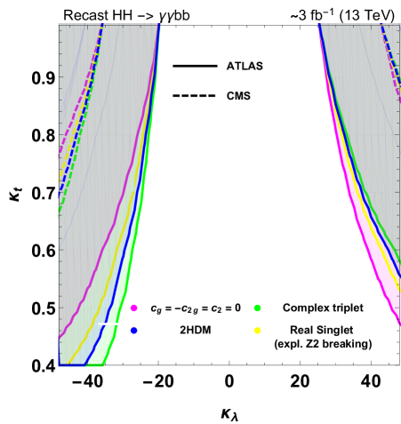
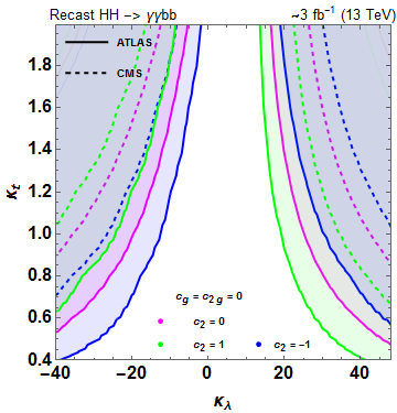
Figure 6: ATLAS (continuous lines) and CMS (dashed lines) 95% exclusion bounds in the $\kappa_{\lambda}-\kappa_{t}$ plane, reinterpreted in terms of different models (left) and in the pure EFT framework for different values of $c_{2}$ (right). See text for details.

Moving to the models which can be described with one parameter (combination), we show in Figure 7 the fiducial cross section as a function of the free (fundamental) parameter for the MCHM (left), real singlet scalar with spontaneous $\mathbb{Z}_{2}$ breaking (center), and singlet vector-like fermion (right) models. For comparison, we also provide current exclusion limits from ATLAS and CMS as well as projections to $100\,$fb^-1, that will exclude the part of the parameter space corresponding to a larger fiducial cross section.

For both MCHM scenarios, the signal efficiency is observed to be rather flat as the kinematics are close to the SM-like case. The sensitivity thus is mostly determined via a simple rescaling of the total rate. The current analyses are sensitive to values of $\xi\sim 0.9$ in the case of the MCHM₅ and values of $\xi\sim 0.2$ can be probed with $100\,$fb^-1, while no bound is obtained for the MCHM₄. We observe a similar pattern in the case of the singlet, where the kinematics are not greatly affected and no bound is obtained for mixing angles $\cos\alpha\gtrsim 0.5$.

In the case of vector-like fermions, the free parameter scales with the Yukawa mixing over the mass of the new states and a decoupling is exhibited with the latter approaching infinity, as expected. As shown in Table 7, the vector-like quark model does not modify $\kappa_{\lambda}$. Combining this with the sensitivity information of Figure 6, it is not surprising that (expected) limits are rather weak, stemming mostly from a non-vanishing $c_{2}$ and residing in the region of large couplings ($\lambda_{Tt}\gtrsim 1$) and/or small masses ($M_{T}\lesssim 1$ TeV). The vector-like leptons, on the other hand, do modify $\kappa_{\lambda}$ and also identically affect $\kappa_{t}$. Since $c_{2}$ is unchanged, they correspond exactly to the benchmark scenario considered in the experimental analyses (with the additional constraint $\kappa_{t}\equiv\kappa_{\lambda}$) and the limits are also rather weak.

Finally, Figure 8 displays the limits obtained for the models with more than one free parameter, this time in terms of the different ’fundamental’ model parameters (and including the real scalar triplet): the real singlet with explicit $\mathbb{Z}_{2}$ symmetry breaking (left), the real/complex triplet (center) and the 2HDM (right). Where possible, we reduce the parameter space to two degrees of freedom: In the triplet models we set the heavy scalar masses to be equal while for the real singlet we can define an effective trilinear coupling

$$\lambda_{\text{eff}}=\lambda_{\alpha}-t_{\alpha}\frac{m_{2}}{v}\,.$$ (10)

In the 2HDM, it is not trivial to reduce the $(t_{\beta},Z_{6},m_{H})$ parameter space. However, $Z_{6}$ is related to the usual alignment parameter, $\cos_{\beta-\alpha}$ and the neutral scalar masses by [39]

$$v^{2}Z_{6}=-\cos_{\beta-\alpha}\sin_{\beta-\alpha}(m_{H}^{2}-m_{h}^{2}),$$ (11)

which we use to fix a relation between the latter, showing predictions for two fixed values of $Z_{6}=\pm 2.5$.

The current constraints on the real singlet lie in regions of large $\lambda_{\text{eff}}$ of order 5–10 and of sizable mixing with the Higgs. The bounds will however improve significantly with increasing luminosity. For the triplets, the analyses are sensitive to large mixings for masses of a few hundred GeV while increasing the heavy scalar mass leads to an increased sensitivity, including also smaller mixing angles $\beta$. This subtle behaviour is due to the fact that $m_{H}^{2}$ is proportional to the size of scalar quartic interactions (times the electroweak vev squared), such that the coupling strength increases with the scalar mass. We thus cut off the parameter space at $m_{H}^{2}\sim 4\pi v^{2}\sim 1$ TeV, in order to remain at a reliable (perturbative) behaviour of the theory. Finally, in the case of the 2HDM, a sensitivity to scalar masses in the TeV region is only possible for small $\tan\beta$, which amplifies the corrections to $\kappa_{t}$ and $c_{2}$.

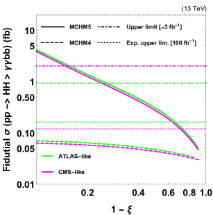
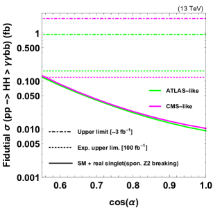
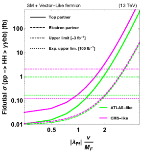
Figure 7: Predictions of the one-parameter models in Table 6 and 95% CL exclusion bounds. See text for details.

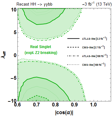
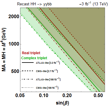
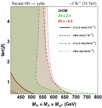
Figure 8: ATLAS (continuous lines) and CMS (dashed lines) 95% exclusion bounds (as well as projected constraints) for different explicit models given in Table 6, as derived in the EFT framework.

6 Mapping between smooth scan and shape benchmarks

Most of the times the experimental searches are not easy to recast as soon as shape analysis or multivariative analysis is used. In this case we may ask ourselves if at some level of confidence we can use results obtained for shape benchmarks for a general study of the parameter space. In this chapter we test this premise on the scans presented in the last chapter. We verify how the same criteria used to define the shape benchmarks as representatives of clusters of similar shapes from a large parameter space scan can help to predict the closest experimental limit (provided there is a list of results for the shape benchmarks), and how this limit can approximate the “real“ limit .

As a quick reminder, in Ref. [10] a two sample Test Statistic (TS) was defined to order the degree of similarity between two samples. The log-likelihood ratio function of the hypothetical case in which the two samples under test share the same parent distribution is the product over the bins of the probability to observe $n_{i,1}$ and $n_{i,2}$ event counts in bin $i$ from the two samples $S_{1}$ and $S_{2}$ and can be written as:

$$TS=-2\sum_{i=1}^{N_{bins}}\left[log(n_{i,1}!)+log(n_{i,2}!)-2log\left(\frac{n_{i,1}+n_{i,2}}{2}!\right)\right]\,.$$ (12)

This quantity is constructed in a manner that it is “$\chi^{2}$ distributed“ [44, 45] and therefore can be directly used as an ordering parameter to decide between pairs of test samples which of them are the most likely to be compatible with the same parental distribution. In other words, the values $TS_{ij}$ and $TS_{kl}$ obtained respectively by testing the compatibility of samples $ij$ and $kl$ are suitable to determine if samples $S_{i}$ and $S_{j}$ are more similar to each other than are samples $S_{k}$ and $S_{l}$: this is the case if $TS_{ij}>TS_{kl}$.

One solution for constructing analyses optimal in continuous scans is, for example, the use the $TS$ as quantity to decide, given a test sample to which shape benchmark this one is most similar to and check if this prediction corresponds to the closest experimental limit. At this point we should emphasise that we are after the closest experimental limit. The real experimental limit, that would be directly derived for the test point, would be a bit different from the one from the closest shape benchmark.

Since we are considering cut-and-count examples the "experimental limits" can be well identified with the signal efficiency in the signal region. As the CMS-like analysis contains a cut in the $m_{\gamma\gamma b\overline{b}}$ variable the signal efficiency is more sensitive to the BSM physics, therefore we will only do this mapping exercise for the CMS-like case. In figures 9 and 10 we show the efficiency maps for the cases of the two 2HDM scans and the triplet and singlet extension cases. Of course the quality of color interpolation on the figures depend on the density of points inspected. To each inspected point a marker is superimposed, symbolizing the closest shape benchmark according to eq. 12. The first fact to notice is that as suggested in [10], the regions belonging to the same benchmark tend to enclose fully connected regions of parameter space, that we will call islands. We also notice that within those fully connected regions the closest benchmark indeed has a signal efficiency that is the closest to the true one. This conclusion is not so precise near the boundaries between islands.

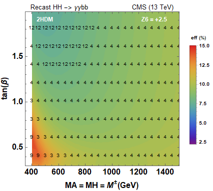
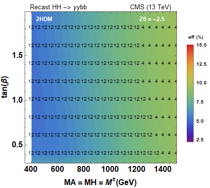
Figure 9: Efficiency maps for the signal region of the CMS-like analysis to the 2HDM benchmarks we consider. The markers superimposed correspond to the closest shape benchmark. Details in the text.

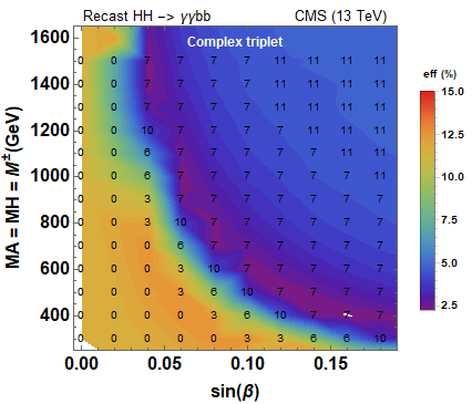
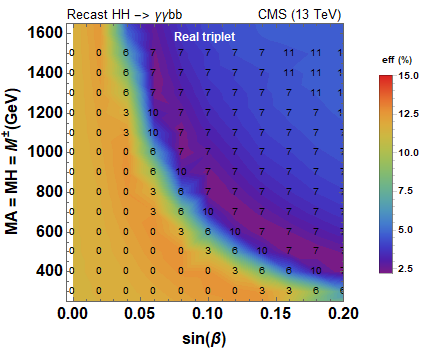
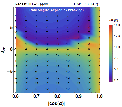
Figure 10: Efficiency maps for the signal region of the CMS-like analysis to the triplet and singlet benchmarks we consider. The markers superimposed correspond to the closest shape benchmark. Details in the text.

This approach has multiple applications: If used by the theory side it is an approximation of reality, that can be employed to obtain a first estimate of the constraints on a specific model without the need to expensive MC simulations or recast. This usage would hold for the case of including further BSM effects such as the inclusion of additional EFT operators (for example, the chromomagnetic term [46]) or the departure from the EFT framework towards explicit inclusion of particles in the loops (for example [47, 48]). On the experimental side usage, we can imagine a situation where it is advantageous for the discovery potential of a hypothetical BSM signal to construct different selections (or multivariate variables) for the different shape benchmarks. In this case it would be unclear how to extend the interpretation of the search to a smooth scan to decide which set of cuts for use to a point that is not a shape benchmark, and the $TS$-test offers a solution for keeping the best search sensitivity also for the case of smooth parameter space scans.

7 Implementation in Rosetta

Although the numerical values of the coefficients that can be used to construct the signal predictions are given in appendix A, for convenience, the input and algorithm to perform sample reweighing are implemented as a module of the Rosetta package [49]. Rosetta provides a framework for EFT basis translations along with a suite of modules ranging from the calculation of Higgs branching fractions via an interface to eHDECAY [50] to the compatibility of a given parameter space point to electroweak precision data and Higgs signal strength measurements. All modules can be exploited in a basis-independent way once a basis definition has be implemented in the package. The package may be found on http://rosetta.hepforge.org/.

The results of this paper are implemented as in extension of the existing dihiggs module [51]. In this module we had implemented the example of usage of the elements of the machinery that do not require expensive Monte Carlo simulations, namely the mapping of parameter space points into shape benchmarks done in the last section. From this implementation it is straightforward for the user to extend it to the case where the calculation of event weights is of interest. After downloading the package, one can invoke the dihiggs interface by calling the command line executable,

>> bin/rosetta dihiggs [OPTIONS]

The package is designed to receive SLHA formatted parameter cards specifying the coefficients of an existing basis implementation. The required translations are then performed to obtain the anomalous Higgs couplings parameters relevant for pair production and decay. Alternatively, one can directly specify the values of the anomalous coupling parameters via the self-explanatory --kl, --kt, --c2, --cg and --c2g optional arguments. The input parameter card has therefore been made optional, to be specified by the --param_card option.

Along with computing the inclusive Higgs pair production cross section, the module will also compute the correct Higgs branching fractions for that point in parameter space using either eHDECAY or an internal interpolating function. Using the results of this paper, we have also added the functionality to return the closest benchmark according to the test defined in formula 12. Finally, the computation of the higgs-pair production process is promoted to differential level, via an internal function. Inside interfaces/dihiggs/AnalyticalReweighter.py the user can find a function weight(variables), where a matrix of weights is calculated from vectors containing the generation level variables $m_{HH}$ and $\cos\theta^{*}$ according to formula 7. Support for implementing the same algorithm in C++ fashion may be given by directly emailing us.

8 Conclusions

Understanding the properties of the Higgs potential is of utmost importance to eventually answer one of the key questions in particle physics, namely what is the origin of EWSB. Examining the production of Higgs pairs is a crucial experiment to achieve this goal, with a focus both on the total cross section, as well as on distributions, which contain valuable information on the nature of potential NP.

In this article we presented semi-analytic results for the distributions of the Higgs-pair production cross section in a well defined and maximally general parametrization of nature, as it appears at low energies, employing EFT. This allows us to express potential deviations from the SM in a consistent way as coefficients of effective operators and constraints on these operators will provide us a guidance on how nature could look at shortest distances.

Furthermore, we employed the formula to recast exclusion bounds, derived assuming certain benchmark points in parameter space with a given kinematics, to points with modified kinematic distributions. The presented method is crucial to cover the full EFT parameter space, taking correctly into account the efficiencies of signal selections.

Finally, the results presented are also useful to confront explicit models, mapped to an EFT, efficiently with constraints from the LHC, providing a bridge between (explicit) theories and data. We demonstrated this procedure, using recent ATLAS and CMS results, for various NP setups, like models with additional scalars, including 2HDM, vector-like fermions, and minimal composite Higgs models, delivering also a dictionary between their explicit parameters and effective couplings after electroweak symmetry breaking.

9 Acknowledgements

FG and AC are grateful for the hospitality of the CERN theory division during the completion of this work. A.C is grateful to Andre Tinoco Mendes, Luca Cadamuro, Giacomo Ortona, Olivier Bondu, Konstantin Androsov, Andrey Pozdnyakov, Rafael Teixeira de Lima, Martino Dall’Osso and Tommaso Dorigo for the fruitful discussions and encouragement to pursue this work. K. M. is supported in part by the Belgian Federal Science Policy Office through the Interuniversity Attraction Pole P7/37 and by the European Union’s Horizon 2020 research and innovation programme under the Marie Skłodowska-Curie grant agreement No. 707983.

Appendix A Numeric tables with the coefficients

Tables 9 to 12 contains the numeric values of the formula 3. The first columns of the tables stand for the number of the bin, followed by the mean $m_{hh}$ and $cos\,\theta^{*}$ of that bin. It is also displayed the number of events found in that bin for a 13,000,000 events SM sample and for the 1,200,000 events of the reweighting sample $\mathcal{S}_{\rm BSM}$ used in this paper. The same informations can be found visually in figures 11 (for the number of events/bin) and 12 (for the values of the coefficients on the not central $cos\,\theta^{*}$ bins).

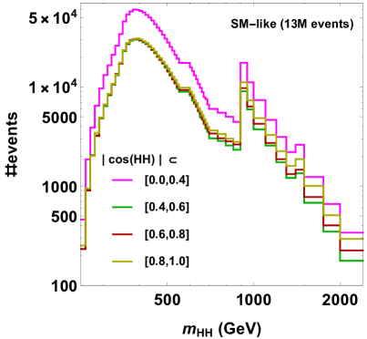
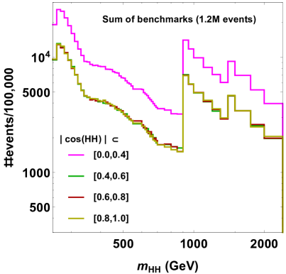
Figure 11: The bin-by-bin statistic of events in a 3M SM sample and on a 1.2M reweighting sample constructed by the plain sum of shape benchmarks.

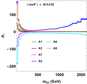
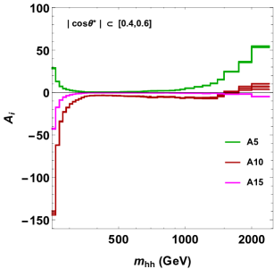
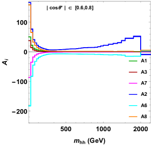
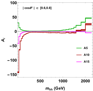
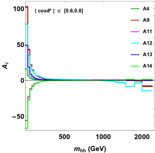
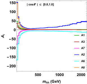
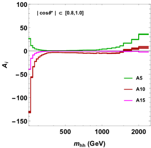
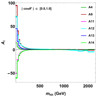
Figure 12: Values of the fit coefficients entering $R_{\rm HH}^{j}$, differential in $m_{HH}$. We only display the results for the central $\cos\theta^{\ast}$ bin (betweem 0 and 0.4). From left to right we show respectivelly the coefficients relative to subspace S1 and S2, S4 and finally S3, S5 and S6 (see table 1).

$j$	$m_{hh}$	$cos\,\theta^{*}$	$N_{SM}^{j}$	$N_{Sum}^{j}$	A1	A2	A3	A4	A5	A6	A7	A8	A9	A10	A11	A12	A13	A14	A15
1	255	0.2	461	19239	4.96E+01	1.73E+02	3.78E+01	1.61E+01	3.07E+01	-1.87E+02	-8.64E+01	1.62E+02	1.06E+02	-1.47E+02	-5.62E+01	7.83E+01	4.93E+01	-6.84E+01	-4.45E+01
2	255	0.5	232	9483	4.86E+01	1.73E+02	3.75E+01	1.60E+01	2.87E+01	-1.85E+02	-8.51E+01	1.61E+02	1.06E+02	-1.42E+02	-5.54E+01	7.44E+01	4.90E+01	-6.50E+01	-4.27E+01
3	255	0.7	233	9604	5.00E+01	1.66E+02	3.75E+01	1.57E+01	2.94E+01	-1.82E+02	-8.65E+01	1.58E+02	1.02E+02	-1.43E+02	-5.61E+01	7.81E+01	4.86E+01	-6.69E+01	-4.31E+01
4	255	0.9	252	9642	4.57E+01	1.52E+02	3.46E+01	1.45E+01	2.62E+01	-1.67E+02	-7.94E+01	1.46E+02	9.41E+01	-1.31E+02	-5.10E+01	7.03E+01	4.47E+01	-6.08E+01	-3.93E+01
5	265	0.2	1862	26019	2.15E+01	7.32E+01	1.35E+01	5.82E+00	1.26E+01	-7.96E+01	-3.40E+01	6.31E+01	4.13E+01	-6.13E+01	-2.23E+01	3.35E+01	1.78E+01	-2.64E+01	-1.72E+01
6	265	0.5	935	13160	2.19E+01	7.27E+01	1.35E+01	5.78E+00	1.30E+01	-8.00E+01	-3.44E+01	6.28E+01	4.10E+01	-6.20E+01	-2.25E+01	3.38E+01	1.77E+01	-2.67E+01	-1.74E+01
7	265	0.7	904	12882	2.23E+01	7.64E+01	1.39E+01	5.91E+00	1.31E+01	-8.28E+01	-3.52E+01	6.53E+01	4.27E+01	-6.45E+01	-2.30E+01	3.44E+01	1.81E+01	-2.72E+01	-1.77E+01
8	265	0.9	947	13002	2.09E+01	7.11E+01	1.32E+01	5.61E+00	1.14E+01	-7.76E+01	-3.31E+01	6.15E+01	4.00E+01	-5.64E+01	-2.14E+01	3.10E+01	1.72E+01	-2.44E+01	-1.58E+01
9	275	0.2	3897	25137	1.26E+01	4.31E+01	6.59E+00	2.83E+00	7.20E+00	-4.68E+01	-1.82E+01	3.39E+01	2.22E+01	-3.54E+01	-1.19E+01	1.92E+01	8.65E+00	-1.38E+01	-9.04E+00
10	275	0.5	2058	12280	1.21E+01	4.14E+01	6.27E+00	2.71E+00	7.20E+00	-4.51E+01	-1.74E+01	3.22E+01	2.11E+01	-3.41E+01	-1.14E+01	1.89E+01	8.25E+00	-1.35E+01	-8.83E+00
11	275	0.7	2023	12088	1.22E+01	4.11E+01	6.36E+00	2.74E+00	6.99E+00	-4.49E+01	-1.75E+01	3.25E+01	2.12E+01	-3.37E+01	-1.15E+01	1.87E+01	8.35E+00	-1.34E+01	-8.74E+00
12	275	0.9	2024	12509	1.22E+01	4.12E+01	6.35E+00	2.76E+00	6.87E+00	-4.49E+01	-1.75E+01	3.25E+01	2.14E+01	-3.38E+01	-1.15E+01	1.85E+01	8.38E+00	-1.33E+01	-8.71E+00
13	285	0.2	6460	21999	8.67E+00	2.99E+01	3.80E+00	1.63E+00	4.65E+00	-3.21E+01	-1.15E+01	2.13E+01	1.39E+01	-2.38E+01	-7.51E+00	1.27E+01	4.98E+00	-8.40E+00	-5.50E+00
14	285	0.5	3245	10960	8.53E+00	2.94E+01	3.76E+00	1.62E+00	4.56E+00	-3.17E+01	-1.13E+01	2.10E+01	1.38E+01	-2.29E+01	-7.39E+00	1.26E+01	4.94E+00	-8.29E+00	-5.42E+00
15	285	0.7	3203	10987	8.69E+00	2.99E+01	3.81E+00	1.64E+00	4.89E+00	-3.21E+01	-1.15E+01	2.14E+01	1.41E+01	-2.46E+01	-7.53E+00	1.31E+01	5.00E+00	-8.64E+00	-5.65E+00
16	285	0.9	3439	10778	8.28E+00	2.74E+01	3.57E+00	1.53E+00	4.32E+00	-2.99E+01	-1.09E+01	1.99E+01	1.29E+01	-2.24E+01	-7.12E+00	1.21E+01	4.69E+00	-7.95E+00	-5.18E+00
17	295	0.2	9651	18825	6.37E+00	2.17E+01	2.35E+00	1.01E+00	3.47E+00	-2.34E+01	-7.72E+00	1.43E+01	9.34E+00	-1.72E+01	-5.04E+00	9.53E+00	3.08E+00	-5.73E+00	-3.72E+00
18	295	0.5	4808	9502	6.43E+00	2.23E+01	2.36E+00	1.01E+00	3.39E+00	-2.40E+01	-7.80E+00	1.45E+01	9.47E+00	-1.76E+01	-5.10E+00	9.40E+00	3.09E+00	-5.68E+00	-3.70E+00
19	295	0.7	4868	9392	6.37E+00	2.18E+01	2.34E+00	9.97E-01	3.43E+00	-2.36E+01	-7.70E+00	1.43E+01	9.33E+00	-1.72E+01	-5.01E+00	9.24E+00	3.05E+00	-5.60E+00	-3.67E+00
20	295	0.9	4920	9420	6.29E+00	2.14E+01	2.30E+00	9.87E-01	3.32E+00	-2.32E+01	-7.59E+00	1.41E+01	9.22E+00	-1.72E+01	-4.98E+00	9.26E+00	3.02E+00	-5.57E+00	-3.63E+00
21	305	0.2	13170	16088	5.07E+00	1.71E+01	1.58E+00	6.62E-01	2.52E+00	-1.86E+01	-5.65E+00	1.04E+01	6.75E+00	-1.31E+01	-3.65E+00	7.24E+00	2.05E+00	-4.02E+00	-2.58E+00
22	305	0.5	6387	8299	5.17E+00	1.77E+01	1.64E+00	6.83E-01	2.59E+00	-1.91E+01	-5.81E+00	1.08E+01	7.00E+00	-1.34E+01	-3.74E+00	7.38E+00	2.12E+00	-4.13E+00	-2.66E+00
23	305	0.7	6631	8002	5.05E+00	1.69E+01	1.57E+00	6.64E-01	2.48E+00	-1.85E+01	-5.63E+00	1.04E+01	6.79E+00	-1.29E+01	-3.66E+00	7.19E+00	2.05E+00	-3.97E+00	-2.56E+00
24	305	0.9	6612	8109	5.06E+00	1.70E+01	1.58E+00	6.49E-01	2.55E+00	-1.85E+01	-5.63E+00	1.04E+01	6.67E+00	-1.33E+01	-3.62E+00	7.23E+00	2.02E+00	-3.99E+00	-2.57E+00
25	315	0.2	16525	13745	4.28E+00	1.46E+01	1.15E+00	4.69E-01	2.04E+00	-1.58E+01	-4.43E+00	8.22E+00	5.25E+00	-1.10E+01	-2.83E+00	6.03E+00	1.47E+00	-3.10E+00	-1.96E+00
26	315	0.5	8236	7014	4.32E+00	1.44E+01	1.16E+00	4.70E-01	2.05E+00	-1.57E+01	-4.49E+00	8.16E+00	5.19E+00	-1.08E+01	-2.85E+00	6.00E+00	1.48E+00	-3.12E+00	-1.98E+00
27	315	0.7	8413	7076	4.23E+00	1.44E+01	1.13E+00	4.55E-01	2.04E+00	-1.56E+01	-4.36E+00	8.06E+00	5.10E+00	-1.08E+01	-2.78E+00	5.94E+00	1.43E+00	-3.03E+00	-1.92E+00
28	315	0.9	8510	7038	4.21E+00	1.43E+01	1.12E+00	4.54E-01	1.94E+00	-1.55E+01	-4.33E+00	8.02E+00	5.10E+00	-1.05E+01	-2.75E+00	5.82E+00	1.43E+00	-3.00E+00	-1.89E+00
29	325	0.2	21078	11797	3.65E+00	1.22E+01	8.32E-01	3.23E-01	1.65E+00	-1.33E+01	-3.48E+00	6.38E+00	3.98E+00	-9.04E+00	-2.17E+00	4.94E+00	1.04E+00	-2.37E+00	-1.47E+00
30	325	0.5	10542	5837	3.64E+00	1.17E+01	8.31E-01	3.22E-01	1.59E+00	-1.31E+01	-3.47E+00	6.26E+00	3.90E+00	-8.86E+00	-2.16E+00	4.95E+00	1.03E+00	-2.37E+00	-1.46E+00
31	325	0.7	10614	5908	3.62E+00	1.19E+01	8.19E-01	3.19E-01	1.58E+00	-1.31E+01	-3.44E+00	6.25E+00	3.89E+00	-8.85E+00	-2.15E+00	4.84E+00	1.02E+00	-2.33E+00	-1.45E+00
32	325	0.9	10752	5900	3.60E+00	1.18E+01	8.07E-01	3.10E-01	1.48E+00	-1.30E+01	-3.40E+00	6.19E+00	3.82E+00	-8.42E+00	-2.12E+00	4.68E+00	1.00E+00	-2.23E+00	-1.38E+00
33	335	0.2	26047	10369	3.19E+00	1.04E+01	6.24E-01	2.31E-01	1.27E+00	-1.15E+01	-2.82E+00	5.10E+00	3.10E+00	-7.31E+00	-1.72E+00	4.05E+00	7.60E-01	-1.80E+00	-1.09E+00
34	335	0.5	13112	5183	3.18E+00	1.04E+01	6.17E-01	2.28E-01	1.27E+00	-1.15E+01	-2.80E+00	5.08E+00	3.08E+00	-7.37E+00	-1.70E+00	4.00E+00	7.50E-01	-1.79E+00	-1.09E+00
35	335	0.7	13521	5144	3.14E+00	1.02E+01	5.99E-01	2.17E-01	1.21E+00	-1.13E+01	-2.73E+00	4.95E+00	2.97E+00	-7.05E+00	-1.66E+00	3.94E+00	7.22E-01	-1.73E+00	-1.04E+00
36	335	0.9	13340	5134	3.16E+00	1.03E+01	6.09E-01	2.25E-01	1.26E+00	-1.14E+01	-2.77E+00	5.01E+00	3.04E+00	-7.19E+00	-1.68E+00	4.01E+00	7.40E-01	-1.77E+00	-1.07E+00
37	345	0.2	34128	9211	2.80E+00	8.81E+00	4.56E-01	1.53E-01	9.71E-01	-9.93E+00	-2.26E+00	4.01E+00	2.32E+00	-5.88E+00	-1.31E+00	3.32E+00	5.28E-01	-1.34E+00	-7.74E-01
38	345	0.5	17291	4591	2.78E+00	8.60E+00	4.47E-01	1.52E-01	9.44E-01	-9.78E+00	-2.23E+00	3.92E+00	2.28E+00	-5.75E+00	-1.30E+00	3.26E+00	5.20E-01	-1.31E+00	-7.64E-01
39	345	0.7	17129	4630	2.79E+00	8.84E+00	4.51E-01	1.53E-01	9.82E-01	-9.93E+00	-2.24E+00	3.99E+00	2.33E+00	-5.89E+00	-1.31E+00	3.29E+00	5.26E-01	-1.33E+00	-7.74E-01
40	345	0.9	17533	4638	2.77E+00	8.61E+00	4.44E-01	1.50E-01	9.50E-01	-9.77E+00	-2.22E+00	3.91E+00	2.26E+00	-5.83E+00	-1.29E+00	3.29E+00	5.15E-01	-1.33E+00	-7.70E-01
41	355	0.2	45693	9105	2.50E+00	7.43E+00	3.37E-01	1.00E-01	7.25E-01	-8.60E+00	-1.83E+00	3.16E+00	1.72E+00	-4.68E+00	-9.97E-01	2.67E+00	3.68E-01	-9.87E-01	-5.40E-01
42	355	0.5	22904	4473	2.49E+00	7.44E+00	3.37E-01	1.01E-01	6.78E-01	-8.61E+00	-1.83E+00	3.17E+00	1.73E+00	-4.57E+00	-1.00E+00	2.67E+00	3.68E-01	-9.81E-01	-5.35E-01
43	355	0.7	23414	4521	2.48E+00	7.23E+00	3.31E-01	9.89E-02	7.09E-01	-8.47E+00	-1.81E+00	3.10E+00	1.69E+00	-4.54E+00	-9.89E-01	2.66E+00	3.61E-01	-9.73E-01	-5.36E-01
44	355	0.9	23458	4508	2.46E+00	7.22E+00	3.26E-01	9.78E-02	7.04E-01	-8.42E+00	-1.79E+00	3.07E+00	1.68E+00	-4.53E+00	-9.78E-01	2.65E+00	3.56E-01	-9.61E-01	-5.27E-01
45	365	0.2	53582	8685	2.31E+00	6.82E+00	2.72E-01	7.55E-02	5.88E-01	-7.93E+00	-1.58E+00	2.73E+00	1.43E+00	-4.01E+00	-8.21E-01	2.32E+00	2.86E-01	-8.02E-01	-4.22E-01
46	365	0.5	26937	4279	2.30E+00	6.73E+00	2.71E-01	7.41E-02	6.14E-01	-7.87E+00	-1.57E+00	2.70E+00	1.40E+00	-4.07E+00	-8.15E-01	2.38E+00	2.82E-01	-8.21E-01	-4.31E-01
47	365	0.7	27395	4265	2.29E+00	6.64E+00	2.66E-01	7.35E-02	5.80E-01	-7.78E+00	-1.55E+00	2.66E+00	1.39E+00	-3.89E+00	-8.08E-01	2.30E+00	2.78E-01	-7.93E-01	-4.16E-01
48	365	0.9	27758	4378	2.28E+00	6.54E+00	2.62E-01	7.16E-02	5.69E-01	-7.71E+00	-1.54E+00	2.62E+00	1.35E+00	-3.91E+00	-7.93E-01	2.28E+00	2.72E-01	-7.80E-01	-4.10E-01
49	375	0.2	57750	8481	2.19E+00	6.64E+00	2.35E-01	6.04E-02	5.44E-01	-7.58E+00	-1.42E+00	2.50E+00	1.26E+00	-3.77E+00	-6.98E-01	2.10E+00	2.36E-01	-7.04E-01	-3.62E-01
50	375	0.5	29067	4355	2.19E+00	6.56E+00	2.34E-01	6.21E-02	5.21E-01	-7.53E+00	-1.42E+00	2.48E+00	1.27E+00	-3.68E+00	-7.15E-01	2.09E+00	2.39E-01	-7.02E-01	-3.64E-01
51	375	0.7	29727	4311	2.17E+00	6.46E+00	2.27E-01	5.92E-02	5.17E-01	-7.46E+00	-1.40E+00	2.43E+00	1.22E+00	-3.66E+00	-6.91E-01	2.09E+00	2.29E-01	-6.91E-01	-3.58E-01
52	375	0.9	29382	4370	2.18E+00	6.48E+00	2.31E-01	6.09E-02	5.36E-01	-7.49E+00	-1.41E+00	2.45E+00	1.24E+00	-3.78E+00	-7.07E-01	2.16E+00	2.34E-01	-7.22E-01	-3.74E-01
53	385	0.2	60252	8527	2.08E+00	6.46E+00	2.02E-01	5.14E-02	5.17E-01	-7.27E+00	-1.28E+00	2.29E+00	1.13E+00	-3.63E+00	-6.09E-01	1.97E+00	1.99E-01	-6.39E-01	-3.31E-01
54	385	0.5	29918	4342	2.09E+00	6.49E+00	2.04E-01	5.12E-02	4.88E-01	-7.30E+00	-1.29E+00	2.30E+00	1.13E+00	-3.64E+00	-6.12E-01	1.96E+00	1.99E-01	-6.43E-01	-3.30E-01
55	385	0.7	30410	4184	2.08E+00	6.35E+00	2.01E-01	5.16E-02	4.84E-01	-7.21E+00	-1.28E+00	2.26E+00	1.12E+00	-3.56E+00	-6.12E-01	1.96E+00	1.98E-01	-6.34E-01	-3.28E-01
56	385	0.9	30534	4336	2.07E+00	6.27E+00	2.01E-01	4.97E-02	4.98E-01	-7.15E+00	-1.27E+00	2.24E+00	1.10E+00	-3.49E+00	-6.00E-01	1.93E+00	1.96E-01	-6.27E-01	-3.18E-01
57	395	0.2	59804	8361	2.01E+00	6.50E+00	1.83E-01	4.41E-02	5.09E-01	-7.14E+00	-1.19E+00	2.18E+00	1.05E+00	-3.51E+00	-5.41E-01	1.86E+00	1.74E-01	-5.94E-01	-3.03E-01
58	395	0.5	30041	4104	2.01E+00	6.44E+00	1.81E-01	4.59E-02	4.82E-01	-7.09E+00	-1.19E+00	2.16E+00	1.05E+00	-3.46E+00	-5.53E-01	1.80E+00	1.76E-01	-5.74E-01	-2.97E-01
59	395	0.7	30417	4176	2.00E+00	6.29E+00	1.78E-01	4.40E-02	4.94E-01	-7.00E+00	-1.17E+00	2.11E+00	1.02E+00	-3.33E+00	-5.38E-01	1.80E+00	1.71E-01	-5.65E-01	-2.93E-01
60	395	0.9	30800	4206	1.99E+00	6.29E+00	1.75E-01	4.43E-02	4.79E-01	-6.98E+00	-1.17E+00	2.10E+00	1.02E+00	-3.34E+00	-5.34E-01	1.77E+00	1.70E-01	-5.56E-01	-2.90E-01

Table 9: Coefficients of equation 4. There $j$ is the bin number and $m_{hh}$ and $cos\,\theta^{*}$ the central values in the bin. $N_{SM}^{j}$ ( $N_{Sum}^{j}$ ) is the number of events in that bin for SM sample (sum of benchmarks) out of 3M (1.2M) events.

$j$	$m_{hh}$	$cos\,\theta^{*}$	$N_{SM}^{j}$	$N_{Sum}^{j}$	A1	A2	A3	A4	A5	A6	A7	A8	A9	A10	A11	A12	A13	A14	A15
61	405	0.2	58279	8303	1.95E+00	6.59E+00	1.65E-01	4.02E-02	4.95E-01	-7.02E+00	-1.11E+00	2.09E+00	9.82E-01	-3.51E+00	-4.88E-01	1.71E+00	1.55E-01	-5.42E-01	-2.85E-01
62	405	0.5	29217	4146	1.95E+00	6.55E+00	1.66E-01	4.08E-02	4.84E-01	-7.03E+00	-1.12E+00	2.09E+00	9.81E-01	-3.46E+00	-4.94E-01	1.73E+00	1.57E-01	-5.48E-01	-2.87E-01
63	405	0.7	29553	4133	1.94E+00	6.51E+00	1.63E-01	4.10E-02	5.06E-01	-6.98E+00	-1.10E+00	2.06E+00	1.00E+00	-3.45E+00	-4.94E-01	1.78E+00	1.56E-01	-5.57E-01	-2.96E-01
64	405	0.9	30212	4148	1.93E+00	6.29E+00	1.60E-01	3.92E-02	4.81E-01	-6.85E+00	-1.09E+00	2.00E+00	9.41E-01	-3.38E+00	-4.76E-01	1.71E+00	1.50E-01	-5.37E-01	-2.81E-01
65	415	0.2	56376	8307	1.89E+00	6.67E+00	1.51E-01	3.77E-02	4.91E-01	-6.93E+00	-1.04E+00	2.01E+00	9.40E-01	-3.55E+00	-4.44E-01	1.64E+00	1.41E-01	-5.16E-01	-2.75E-01
66	415	0.5	28125	3992	1.90E+00	6.64E+00	1.52E-01	3.63E-02	5.18E-01	-6.95E+00	-1.05E+00	2.01E+00	9.21E-01	-3.54E+00	-4.38E-01	1.59E+00	1.39E-01	-5.11E-01	-2.73E-01
67	415	0.7	28448	4191	1.89E+00	6.57E+00	1.48E-01	3.72E-02	4.88E-01	-6.88E+00	-1.03E+00	1.98E+00	9.21E-01	-3.41E+00	-4.44E-01	1.62E+00	1.39E-01	-4.95E-01	-2.65E-01
68	415	0.9	28836	4239	1.88E+00	6.53E+00	1.46E-01	3.44E-02	4.99E-01	-6.88E+00	-1.03E+00	1.96E+00	8.99E-01	-3.39E+00	-4.31E-01	1.63E+00	1.34E-01	-5.04E-01	-2.64E-01
69	425	0.2	53180	7880	1.85E+00	6.81E+00	1.39E-01	3.46E-02	4.83E-01	-6.89E+00	-9.85E-01	1.95E+00	8.91E-01	-3.44E+00	-4.00E-01	1.56E+00	1.27E-01	-4.92E-01	-2.68E-01
70	425	0.5	27049	3953	1.84E+00	6.70E+00	1.37E-01	3.18E-02	5.02E-01	-6.83E+00	-9.77E-01	1.93E+00	8.69E-01	-3.40E+00	-3.85E-01	1.52E+00	1.21E-01	-4.77E-01	-2.55E-01
71	425	0.7	27261	4078	1.83E+00	6.74E+00	1.34E-01	3.31E-02	4.98E-01	-6.86E+00	-9.68E-01	1.91E+00	8.76E-01	-3.43E+00	-3.93E-01	1.55E+00	1.22E-01	-4.77E-01	-2.59E-01
72	425	0.9	27770	3992	1.84E+00	6.58E+00	1.35E-01	3.38E-02	4.73E-01	-6.80E+00	-9.70E-01	1.89E+00	8.65E-01	-3.39E+00	-4.03E-01	1.53E+00	1.24E-01	-4.67E-01	-2.53E-01
73	435	0.2	50181	7864	1.81E+00	6.99E+00	1.29E-01	3.20E-02	5.24E-01	-6.89E+00	-9.34E-01	1.90E+00	8.51E-01	-3.44E+00	-3.60E-01	1.48E+00	1.15E-01	-4.66E-01	-2.62E-01
74	435	0.5	25410	3949	1.80E+00	6.94E+00	1.28E-01	3.30E-02	5.03E-01	-6.84E+00	-9.30E-01	1.89E+00	8.65E-01	-3.54E+00	-3.74E-01	1.53E+00	1.17E-01	-4.76E-01	-2.66E-01
75	435	0.7	25549	3945	1.80E+00	6.88E+00	1.27E-01	3.19E-02	4.98E-01	-6.84E+00	-9.29E-01	1.88E+00	8.43E-01	-3.32E+00	-3.70E-01	1.53E+00	1.15E-01	-4.77E-01	-2.65E-01
76	435	0.9	25962	3981	1.79E+00	6.70E+00	1.23E-01	3.10E-02	5.02E-01	-6.72E+00	-9.13E-01	1.82E+00	8.37E-01	-3.26E+00	-3.60E-01	1.51E+00	1.11E-01	-4.63E-01	-2.58E-01
77	445	0.2	46676	7830	1.77E+00	7.25E+00	1.21E-01	2.93E-02	5.44E-01	-6.89E+00	-8.90E-01	1.88E+00	8.25E-01	-3.53E+00	-3.25E-01	1.40E+00	1.05E-01	-4.48E-01	-2.57E-01
78	445	0.5	23501	3816	1.76E+00	7.21E+00	1.19E-01	3.15E-02	5.23E-01	-6.88E+00	-8.82E-01	1.85E+00	8.50E-01	-3.55E+00	-3.37E-01	1.40E+00	1.07E-01	-4.46E-01	-2.60E-01
79	445	0.7	23756	3781	1.76E+00	7.05E+00	1.18E-01	3.15E-02	5.31E-01	-6.83E+00	-8.83E-01	1.83E+00	8.19E-01	-3.52E+00	-3.48E-01	1.49E+00	1.08E-01	-4.59E-01	-2.64E-01
80	445	0.9	24417	3888	1.75E+00	6.88E+00	1.14E-01	2.91E-02	4.99E-01	-6.73E+00	-8.67E-01	1.77E+00	7.96E-01	-3.50E+00	-3.35E-01	1.45E+00	1.01E-01	-4.34E-01	-2.46E-01
81	455	0.2	42819	7511	1.74E+00	7.53E+00	1.14E-01	3.16E-02	5.87E-01	-6.95E+00	-8.55E-01	1.86E+00	8.38E-01	-3.70E+00	-3.26E-01	1.44E+00	1.05E-01	-4.58E-01	-2.74E-01
82	455	0.5	21866	3773	1.73E+00	7.40E+00	1.09E-01	2.89E-02	5.63E-01	-6.84E+00	-8.37E-01	1.81E+00	8.16E-01	-3.50E+00	-3.05E-01	1.33E+00	9.68E-02	-4.15E-01	-2.51E-01
83	455	0.7	22275	3770	1.74E+00	7.30E+00	1.10E-01	2.87E-02	5.99E-01	-6.87E+00	-8.46E-01	1.80E+00	8.17E-01	-3.52E+00	-3.20E-01	1.47E+00	9.85E-02	-4.50E-01	-2.65E-01
84	455	0.9	22753	3793	1.72E+00	7.10E+00	1.05E-01	2.95E-02	4.97E-01	-6.74E+00	-8.24E-01	1.72E+00	7.83E-01	-3.52E+00	-3.13E-01	1.35E+00	9.50E-02	-4.04E-01	-2.44E-01
85	465	0.2	39481	7354	1.71E+00	7.78E+00	1.07E-01	2.87E-02	6.14E-01	-7.01E+00	-8.19E-01	1.82E+00	8.13E-01	-3.69E+00	-2.90E-01	1.37E+00	9.40E-02	-4.32E-01	-2.66E-01
86	465	0.5	20095	3678	1.70E+00	7.61E+00	1.04E-01	2.70E-02	5.67E-01	-6.88E+00	-8.08E-01	1.79E+00	7.65E-01	-3.52E+00	-2.76E-01	1.28E+00	8.90E-02	-4.09E-01	-2.49E-01
87	465	0.7	20239	3716	1.69E+00	7.62E+00	1.02E-01	2.75E-02	5.98E-01	-6.88E+00	-7.97E-01	1.78E+00	7.88E-01	-3.68E+00	-2.72E-01	1.31E+00	8.86E-02	-4.10E-01	-2.56E-01
88	465	0.9	20845	3561	1.70E+00	7.37E+00	1.02E-01	2.71E-02	5.78E-01	-6.82E+00	-8.04E-01	1.73E+00	7.63E-01	-3.53E+00	-2.91E-01	1.34E+00	8.85E-02	-4.15E-01	-2.58E-01
89	475	0.2	36626	7301	1.68E+00	8.04E+00	9.92E-02	2.77E-02	6.41E-01	-7.01E+00	-7.77E-01	1.80E+00	7.93E-01	-3.85E+00	-2.58E-01	1.30E+00	8.59E-02	-4.25E-01	-2.73E-01
90	475	0.5	18719	3471	1.66E+00	7.79E+00	9.50E-02	2.77E-02	6.23E-01	-6.86E+00	-7.56E-01	1.73E+00	7.59E-01	-3.83E+00	-2.59E-01	1.26E+00	8.41E-02	-4.10E-01	-2.63E-01
91	475	0.7	18720	3577	1.67E+00	7.74E+00	9.74E-02	2.71E-02	6.18E-01	-6.89E+00	-7.69E-01	1.75E+00	7.61E-01	-3.56E+00	-2.53E-01	1.25E+00	8.37E-02	-4.03E-01	-2.60E-01
92	475	0.9	19475	3528	1.66E+00	7.56E+00	9.27E-02	2.57E-02	6.43E-01	-6.80E+00	-7.53E-01	1.68E+00	7.52E-01	-3.66E+00	-2.54E-01	1.29E+00	8.07E-02	-3.95E-01	-2.56E-01
93	485	0.2	33567	6891	1.66E+00	8.20E+00	9.44E-02	2.72E-02	6.87E-01	-7.00E+00	-7.51E-01	1.76E+00	7.65E-01	-3.89E+00	-2.38E-01	1.27E+00	8.05E-02	-4.22E-01	-2.81E-01
94	485	0.5	17086	3503	1.65E+00	8.14E+00	9.01E-02	2.51E-02	6.31E-01	-6.96E+00	-7.35E-01	1.72E+00	7.57E-01	-3.67E+00	-2.29E-01	1.15E+00	7.46E-02	-3.83E-01	-2.55E-01
95	485	0.7	17444	3473	1.65E+00	7.88E+00	9.22E-02	2.71E-02	6.45E-01	-6.87E+00	-7.39E-01	1.72E+00	7.39E-01	-3.69E+00	-2.44E-01	1.25E+00	8.03E-02	-4.05E-01	-2.67E-01
96	485	0.9	17889	3453	1.65E+00	7.74E+00	8.88E-02	2.57E-02	6.32E-01	-6.83E+00	-7.35E-01	1.67E+00	7.25E-01	-3.60E+00	-2.54E-01	1.31E+00	7.70E-02	-4.05E-01	-2.64E-01
97	495	0.2	30583	6650	1.63E+00	8.50E+00	8.81E-02	2.71E-02	7.01E-01	-7.07E+00	-7.20E-01	1.74E+00	7.43E-01	-4.01E+00	-2.28E-01	1.15E+00	7.63E-02	-3.89E-01	-2.75E-01
98	495	0.5	15630	3332	1.62E+00	8.42E+00	8.51E-02	2.55E-02	7.09E-01	-7.03E+00	-7.04E-01	1.71E+00	7.38E-01	-3.91E+00	-2.15E-01	1.18E+00	7.27E-02	-3.83E-01	-2.64E-01
99	495	0.7	16167	3422	1.62E+00	8.12E+00	8.43E-02	2.67E-02	6.75E-01	-6.93E+00	-7.05E-01	1.67E+00	7.46E-01	-3.58E+00	-2.27E-01	1.19E+00	7.45E-02	-3.76E-01	-2.64E-01
100	495	0.9	16559	3360	1.61E+00	7.97E+00	8.24E-02	2.45E-02	6.04E-01	-6.84E+00	-6.96E-01	1.64E+00	6.93E-01	-3.66E+00	-2.19E-01	1.19E+00	6.94E-02	-3.64E-01	-2.50E-01
101	505	0.2	27997	6594	1.61E+00	8.88E+00	8.44E-02	2.49E-02	7.67E-01	-7.14E+00	-6.93E-01	1.75E+00	7.18E-01	-3.98E+00	-1.91E-01	1.13E+00	6.90E-02	-3.88E-01	-2.79E-01
102	505	0.5	14226	3210	1.60E+00	8.68E+00	8.12E-02	2.36E-02	7.12E-01	-7.08E+00	-6.82E-01	1.69E+00	7.27E-01	-3.85E+00	-1.82E-01	1.00E+00	6.42E-02	-3.53E-01	-2.62E-01
103	505	0.7	14414	3214	1.60E+00	8.65E+00	8.08E-02	2.64E-02	7.03E-01	-7.07E+00	-6.84E-01	1.70E+00	7.28E-01	-3.92E+00	-2.16E-01	1.20E+00	7.09E-02	-3.83E-01	-2.74E-01
104	505	0.9	15322	3179	1.59E+00	8.07E+00	7.66E-02	2.36E-02	6.92E-01	-6.89E+00	-6.69E-01	1.59E+00	6.72E-01	-3.81E+00	-2.00E-01	1.12E+00	6.34E-02	-3.52E-01	-2.58E-01
105	515	0.2	25283	6251	1.60E+00	9.27E+00	8.12E-02	2.63E-02	8.25E-01	-7.29E+00	-6.78E-01	1.76E+00	7.08E-01	-4.13E+00	-1.91E-01	1.09E+00	6.81E-02	-3.94E-01	-2.97E-01
106	515	0.5	12999	3224	1.59E+00	8.94E+00	7.86E-02	2.34E-02	8.22E-01	-7.11E+00	-6.67E-01	1.72E+00	7.04E-01	-4.01E+00	-1.85E-01	1.09E+00	6.41E-02	-3.72E-01	-2.81E-01
107	515	0.7	13375	3082	1.58E+00	8.80E+00	7.52E-02	2.24E-02	7.30E-01	-7.07E+00	-6.55E-01	1.64E+00	6.82E-01	-3.78E+00	-1.73E-01	1.11E+00	5.93E-02	-3.55E-01	-2.58E-01
108	515	0.9	13918	3122	1.58E+00	8.34E+00	7.29E-02	2.33E-02	7.45E-01	-6.89E+00	-6.52E-01	1.58E+00	6.53E-01	-3.87E+00	-1.98E-01	1.04E+00	6.14E-02	-3.37E-01	-2.59E-01
109	525	0.2	23150	6002	1.57E+00	9.56E+00	7.63E-02	2.35E-02	8.11E-01	-7.29E+00	-6.48E-01	1.73E+00	7.18E-01	-4.11E+00	-1.62E-01	1.01E+00	6.09E-02	-3.58E-01	-2.77E-01
110	525	0.5	11867	2985	1.57E+00	9.19E+00	7.43E-02	2.29E-02	8.29E-01	-7.11E+00	-6.43E-01	1.69E+00	6.33E-01	-4.01E+00	-1.68E-01	1.01E+00	5.93E-02	-3.64E-01	-2.77E-01
111	525	0.7	11919	3060	1.58E+00	9.18E+00	7.47E-02	2.38E-02	8.38E-01	-7.20E+00	-6.51E-01	1.68E+00	6.78E-01	-4.00E+00	-1.78E-01	1.08E+00	6.15E-02	-3.69E-01	-2.85E-01
112	525	0.9	12678	3024	1.56E+00	8.79E+00	7.06E-02	2.03E-02	7.84E-01	-7.04E+00	-6.32E-01	1.59E+00	6.51E-01	-3.78E+00	-1.67E-01	1.07E+00	5.40E-02	-3.38E-01	-2.57E-01
113	535	0.2	21003	5873	1.56E+00	9.97E+00	7.24E-02	2.46E-02	9.18E-01	-7.37E+00	-6.29E-01	1.74E+00	7.09E-01	-4.29E+00	-1.48E-01	9.94E-01	5.85E-02	-3.71E-01	-3.05E-01
114	535	0.5	10788	2875	1.56E+00	9.50E+00	7.28E-02	2.41E-02	8.73E-01	-7.20E+00	-6.34E-01	1.66E+00	6.58E-01	-4.16E+00	-1.56E-01	9.26E-01	5.82E-02	-3.59E-01	-2.96E-01
115	535	0.7	11040	2912	1.56E+00	9.31E+00	7.09E-02	2.49E-02	8.52E-01	-7.20E+00	-6.28E-01	1.66E+00	6.70E-01	-3.94E+00	-1.63E-01	1.02E+00	5.88E-02	-3.59E-01	-2.94E-01
116	535	0.9	11742	2872	1.54E+00	8.95E+00	6.58E-02	2.17E-02	8.09E-01	-7.07E+00	-6.10E-01	1.57E+00	6.72E-01	-3.87E+00	-1.49E-01	9.72E-01	5.17E-02	-3.26E-01	-2.68E-01
117	545	0.2	19327	5631	1.55E+00	1.03E+01	7.02E-02	2.47E-02	9.57E-01	-7.44E+00	-6.18E-01	1.73E+00	7.20E-01	-4.36E+00	-1.46E-01	9.50E-01	5.64E-02	-3.65E-01	-3.10E-01
118	545	0.5	9660	2819	1.54E+00	1.01E+01	6.80E-02	2.34E-02	8.68E-01	-7.38E+00	-6.06E-01	1.69E+00	6.43E-01	-4.26E+00	-1.41E-01	8.97E-01	5.34E-02	-3.33E-01	-2.80E-01
119	545	0.7	10006	2814	1.54E+00	9.64E+00	6.67E-02	2.13E-02	9.98E-01	-7.21E+00	-6.03E-01	1.62E+00	6.75E-01	-4.28E+00	-1.48E-01	1.02E+00	5.24E-02	-3.55E-01	-2.95E-01
120	545	0.9	10606	2817	1.53E+00	9.20E+00	6.24E-02	2.15E-02	8.68E-01	-7.10E+00	-5.89E-01	1.55E+00	6.24E-01	-4.00E+00	-1.40E-01	9.53E-01	4.91E-02	-3.16E-01	-2.74E-01

Table 10: Coefficients of equation 4. There $j$ is the bin number and $m_{hh}$ and $cos\,\theta^{*}$ the central values in the bin. $N_{SM}^{j}$ ( $N_{Sum}^{j}$ ) is the number of events in that bin for SM sample (sum of benchmarks) out of 3M (1.2M) events.

$j$	$m_{hh}$	$cos\,\theta^{*}$	$N_{SM}^{j}$	$N_{Sum}^{j}$	A1	A2	A3	A4	A5	A6	A7	A8	A9	A10	A11	A12	A13	A14	A15
121	555	0.2	17431	5293	1.53E+00	1.06E+01	6.71E-02	2.41E-02	9.93E-01	-7.53E+00	-5.95E-01	1.72E+00	6.88E-01	-4.61E+00	-1.22E-01	7.89E-01	5.29E-02	-3.38E-01	-3.10E-01
122	555	0.5	8936	2644	1.52E+00	1.04E+01	6.48E-02	2.38E-02	1.02E+00	-7.48E+00	-5.87E-01	1.67E+00	7.05E-01	-4.35E+00	-1.18E-01	8.55E-01	5.04E-02	-3.37E-01	-3.09E-01
123	555	0.7	9328	2799	1.51E+00	9.88E+00	6.08E-02	2.43E-02	8.84E-01	-7.27E+00	-5.75E-01	1.57E+00	6.48E-01	-3.98E+00	-1.43E-01	9.36E-01	5.16E-02	-3.37E-01	-2.93E-01
124	555	0.9	9834	2680	1.51E+00	9.28E+00	5.80E-02	2.09E-02	9.79E-01	-7.04E+00	-5.67E-01	1.48E+00	6.08E-01	-3.85E+00	-1.43E-01	9.15E-01	4.67E-02	-3.14E-01	-2.84E-01
125	565	0.2	15754	5247	1.51E+00	1.10E+01	6.33E-02	2.38E-02	1.07E+00	-7.57E+00	-5.76E-01	1.72E+00	6.82E-01	-4.65E+00	-1.05E-01	8.20E-01	4.84E-02	-3.42E-01	-3.22E-01
126	565	0.5	8163	2570	1.50E+00	1.09E+01	6.12E-02	2.48E-02	1.05E+00	-7.52E+00	-5.64E-01	1.70E+00	6.72E-01	-4.56E+00	-1.23E-01	7.31E-01	5.08E-02	-3.33E-01	-3.25E-01
127	565	0.7	8475	2591	1.50E+00	1.02E+01	5.91E-02	2.19E-02	9.23E-01	-7.32E+00	-5.63E-01	1.57E+00	5.92E-01	-4.14E+00	-1.25E-01	8.35E-01	4.51E-02	-3.02E-01	-2.82E-01
128	565	0.9	8926	2521	1.49E+00	9.65E+00	5.48E-02	1.77E-02	9.59E-01	-7.18E+00	-5.46E-01	1.48E+00	5.70E-01	-3.98E+00	-1.18E-01	8.91E-01	3.90E-02	-2.88E-01	-2.68E-01
129	575	0.2	14425	4932	1.51E+00	1.13E+01	6.29E-02	2.49E-02	1.13E+00	-7.61E+00	-5.72E-01	1.71E+00	6.31E-01	-4.68E+00	-1.17E-01	7.71E-01	5.00E-02	-3.38E-01	-3.34E-01
130	575	0.5	7293	2435	1.50E+00	1.08E+01	6.15E-02	2.50E-02	1.08E+00	-7.51E+00	-5.66E-01	1.66E+00	6.25E-01	-4.33E+00	-1.30E-01	8.36E-01	5.05E-02	-3.41E-01	-3.18E-01
131	575	0.7	7724	2447	1.49E+00	1.06E+01	5.58E-02	2.14E-02	1.14E+00	-7.44E+00	-5.47E-01	1.57E+00	5.71E-01	-4.47E+00	-9.68E-02	7.42E-01	3.99E-02	-3.02E-01	-3.14E-01
132	575	0.9	8263	2514	1.48E+00	9.63E+00	5.31E-02	2.22E-02	1.02E+00	-7.16E+00	-5.32E-01	1.47E+00	5.56E-01	-3.84E+00	-1.20E-01	9.35E-01	4.39E-02	-3.25E-01	-3.05E-01
133	585	0.2	13097	4793	1.49E+00	1.17E+01	5.81E-02	2.40E-02	1.24E+00	-7.66E+00	-5.49E-01	1.70E+00	6.45E-01	-4.87E+00	-1.01E-01	7.38E-01	4.56E-02	-3.36E-01	-3.44E-01
134	585	0.5	6752	2365	1.48E+00	1.13E+01	5.67E-02	2.03E-02	1.14E+00	-7.63E+00	-5.32E-01	1.64E+00	6.12E-01	-4.50E+00	-7.31E-02	6.76E-01	3.94E-02	-3.06E-01	-3.04E-01
135	585	0.7	6994	2431	1.48E+00	1.09E+01	5.24E-02	1.82E-02	1.21E+00	-7.46E+00	-5.28E-01	1.57E+00	6.15E-01	-4.38E+00	-7.73E-02	6.89E-01	3.29E-02	-2.85E-01	-3.05E-01
136	585	0.9	7315	2349	1.46E+00	1.04E+01	4.92E-02	2.17E-02	1.18E+00	-7.31E+00	-5.14E-01	1.51E+00	5.77E-01	-4.13E+00	-1.10E-01	8.55E-01	3.96E-02	-3.15E-01	-3.16E-01
137	595	0.2	11949	4652	1.47E+00	1.21E+01	5.55E-02	2.30E-02	1.37E+00	-7.78E+00	-5.28E-01	1.70E+00	5.97E-01	-5.07E+00	-7.11E-02	6.46E-01	4.09E-02	-3.24E-01	-3.57E-01
138	595	0.5	6266	2399	1.47E+00	1.15E+01	5.21E-02	2.29E-02	1.26E+00	-7.55E+00	-5.23E-01	1.61E+00	5.39E-01	-4.96E+00	-7.91E-02	7.21E-01	3.92E-02	-3.19E-01	-3.41E-01
139	595	0.7	6356	2287	1.47E+00	1.16E+01	5.06E-02	1.72E-02	1.21E+00	-7.77E+00	-5.17E-01	1.61E+00	6.62E-01	-4.40E+00	-6.27E-02	5.85E-01	2.91E-02	-2.66E-01	-2.98E-01
140	595	0.9	6860	2229	1.46E+00	1.04E+01	4.72E-02	1.88E-02	1.25E+00	-7.35E+00	-5.07E-01	1.46E+00	5.73E-01	-3.98E+00	-9.44E-02	6.98E-01	3.31E-02	-2.78E-01	-3.11E-01
141	605	0.2	10709	4428	1.48E+00	1.28E+01	5.66E-02	2.19E-02	1.45E+00	-8.02E+00	-5.40E-01	1.76E+00	6.54E-01	-4.87E+00	-7.05E-02	5.46E-01	3.88E-02	-3.19E-01	-3.63E-01
142	605	0.5	5642	2169	1.45E+00	1.18E+01	5.03E-02	2.13E-02	1.33E+00	-7.56E+00	-5.02E-01	1.60E+00	6.07E-01	-4.45E+00	-5.30E-02	6.19E-01	3.52E-02	-3.00E-01	-3.43E-01
143	605	0.7	5791	2178	1.45E+00	1.17E+01	4.84E-02	2.33E-02	1.36E+00	-7.68E+00	-5.02E-01	1.59E+00	6.16E-01	-5.01E+00	-9.17E-02	8.45E-01	3.89E-02	-3.51E-01	-3.63E-01
144	605	0.9	6135	2211	1.46E+00	1.11E+01	4.86E-02	2.38E-02	1.20E+00	-7.59E+00	-5.08E-01	1.49E+00	6.21E-01	-4.40E+00	-9.10E-02	8.26E-01	3.78E-02	-3.04E-01	-3.35E-01
145	615	0.2	9790	4281	1.46E+00	1.31E+01	5.11E-02	2.42E-02	1.48E+00	-7.96E+00	-5.07E-01	1.72E+00	6.50E-01	-5.26E+00	-4.91E-02	5.54E-01	3.73E-02	-3.28E-01	-3.77E-01
146	615	0.5	4916	2161	1.44E+00	1.27E+01	4.85E-02	2.31E-02	1.53E+00	-7.84E+00	-4.86E-01	1.65E+00	6.20E-01	-5.02E+00	-5.46E-02	5.66E-01	3.78E-02	-3.26E-01	-3.77E-01
147	615	0.7	5332	2255	1.42E+00	1.18E+01	4.26E-02	2.18E-02	1.32E+00	-7.60E+00	-4.64E-01	1.51E+00	5.63E-01	-4.66E+00	-6.89E-02	5.66E-01	3.29E-02	-2.71E-01	-3.33E-01
148	615	0.9	5649	2037	1.43E+00	1.13E+01	4.39E-02	1.99E-02	1.32E+00	-7.60E+00	-4.78E-01	1.47E+00	4.68E-01	-4.41E+00	-6.24E-02	6.00E-01	3.06E-02	-2.64E-01	-3.27E-01
149	625	0.2	8863	4128	1.44E+00	1.37E+01	4.95E-02	2.22E-02	1.63E+00	-8.10E+00	-4.91E-01	1.71E+00	6.33E-01	-5.34E+00	-4.42E-02	4.71E-01	3.54E-02	-3.08E-01	-3.80E-01
150	625	0.5	4656	2129	1.43E+00	1.28E+01	4.48E-02	2.45E-02	1.53E+00	-7.85E+00	-4.75E-01	1.63E+00	5.89E-01	-5.05E+00	-5.95E-02	5.67E-01	3.42E-02	-3.02E-01	-3.83E-01
151	625	0.7	4759	2053	1.44E+00	1.26E+01	4.77E-02	2.17E-02	1.55E+00	-8.01E+00	-4.90E-01	1.56E+00	5.74E-01	-4.96E+00	-6.23E-02	6.95E-01	3.43E-02	-3.12E-01	-3.74E-01
152	625	0.9	5211	2089	1.42E+00	1.13E+01	4.11E-02	1.65E-02	1.40E+00	-7.56E+00	-4.59E-01	1.45E+00	4.46E-01	-4.14E+00	-6.08E-02	5.80E-01	2.74E-02	-2.52E-01	-3.10E-01
153	635	0.2	7896	3959	1.45E+00	1.44E+01	5.19E-02	2.34E-02	1.67E+00	-8.33E+00	-5.04E-01	1.78E+00	6.19E-01	-5.35E+00	-5.67E-02	4.37E-01	3.79E-02	-3.08E-01	-3.90E-01
154	635	0.5	4220	1939	1.44E+00	1.36E+01	4.69E-02	2.27E-02	1.60E+00	-8.04E+00	-4.83E-01	1.69E+00	6.45E-01	-5.29E+00	-4.83E-02	3.12E-01	3.29E-02	-2.70E-01	-3.75E-01
155	635	0.7	4356	1945	1.44E+00	1.31E+01	4.35E-02	2.24E-02	1.55E+00	-8.18E+00	-4.80E-01	1.59E+00	6.00E-01	-5.13E+00	-5.89E-02	6.41E-01	3.02E-02	-3.08E-01	-3.73E-01
156	635	0.9	4743	1911	1.43E+00	1.17E+01	4.19E-02	1.49E-02	1.42E+00	-7.56E+00	-4.68E-01	1.45E+00	4.57E-01	-4.24E+00	-4.78E-02	5.20E-01	2.28E-02	-2.36E-01	-3.05E-01
157	645	0.2	7540	3806	1.42E+00	1.41E+01	4.54E-02	2.12E-02	1.80E+00	-8.25E+00	-4.69E-01	1.66E+00	6.08E-01	-5.03E+00	-8.73E-03	1.68E-01	2.65E-02	-2.84E-01	-4.06E-01
158	645	0.5	3796	2001	1.42E+00	1.42E+01	4.34E-02	2.34E-02	1.84E+00	-8.33E+00	-4.63E-01	1.72E+00	5.74E-01	-5.82E+00	-1.78E-02	4.85E-01	2.82E-02	-3.19E-01	-4.14E-01
159	645	0.7	4006	1980	1.41E+00	1.31E+01	3.98E-02	1.71E-02	1.69E+00	-8.02E+00	-4.48E-01	1.49E+00	5.69E-01	-4.42E+00	-3.03E-02	5.18E-01	2.28E-02	-2.87E-01	-3.69E-01
160	645	0.9	4319	1872	1.40E+00	1.23E+01	3.60E-02	2.03E-02	1.47E+00	-7.91E+00	-4.32E-01	1.43E+00	4.38E-01	-4.37E+00	-5.54E-02	3.44E-01	2.52E-02	-2.33E-01	-3.45E-01
161	655	0.2	6638	3673	1.43E+00	1.51E+01	4.67E-02	2.80E-02	1.94E+00	-8.42E+00	-4.73E-01	1.75E+00	6.28E-01	-5.23E+00	-4.88E-02	4.28E-01	3.97E-02	-3.38E-01	-4.53E-01
162	655	0.5	3507	1804	1.42E+00	1.42E+01	4.19E-02	3.02E-02	1.75E+00	-8.15E+00	-4.62E-01	1.60E+00	6.40E-01	-4.96E+00	-7.58E-02	4.21E-01	4.02E-02	-3.18E-01	-4.35E-01
163	655	0.7	3668	1888	1.46E+00	1.36E+01	4.33E-02	1.45E-02	1.82E+00	-8.24E+00	-5.06E-01	1.63E+00	4.69E-01	-5.07E+00	-8.88E-02	4.32E-01	2.08E-02	-2.81E-01	-3.69E-01
164	655	0.9	3969	1825	1.48E+00	1.27E+01	4.68E-02	1.65E-02	1.72E+00	-8.17E+00	-5.30E-01	1.61E+00	4.84E-01	-4.28E+00	-9.67E-02	6.98E-01	2.53E-02	-2.72E-01	-3.67E-01
165	665	0.2	6000	3577	1.41E+00	1.55E+01	4.37E-02	2.53E-02	2.07E+00	-8.53E+00	-4.57E-01	1.69E+00	5.24E-01	-5.26E+00	-1.88E-02	5.19E-02	3.07E-02	-2.79E-01	-4.47E-01
166	665	0.5	3031	1740	1.43E+00	1.52E+01	3.69E-02	2.52E-02	1.93E+00	-8.46E+00	-4.71E-01	1.66E+00	5.07E-01	-5.78E+00	-4.99E-02	3.75E-01	2.45E-02	-2.84E-01	-4.50E-01
167	665	0.7	3389	1743	1.39E+00	1.39E+01	3.63E-02	2.04E-02	1.84E+00	-8.09E+00	-4.27E-01	1.50E+00	5.23E-01	-4.69E+00	-4.85E-02	4.89E-01	2.67E-02	-3.10E-01	-4.05E-01
168	665	0.9	3643	1730	1.38E+00	1.29E+01	3.02E-02	2.49E-02	1.79E+00	-8.04E+00	-4.09E-01	1.38E+00	5.80E-01	-4.84E+00	-6.70E-02	3.99E-01	2.79E-02	-2.62E-01	-3.99E-01
169	675	0.2	5498	3478	1.41E+00	1.63E+01	4.32E-02	2.58E-02	2.26E+00	-8.77E+00	-4.50E-01	1.71E+00	6.15E-01	-5.98E+00	1.29E-02	1.17E-01	2.82E-02	-2.97E-01	-4.86E-01
170	675	0.5	2857	1747	1.39E+00	1.53E+01	3.69E-02	2.23E-02	2.14E+00	-8.42E+00	-4.23E-01	1.59E+00	5.29E-01	-5.00E+00	-1.17E-02	9.29E-02	2.27E-02	-2.79E-01	-4.59E-01
171	675	0.7	3037	1762	1.38E+00	1.44E+01	3.59E-02	1.41E-02	1.88E+00	-8.22E+00	-4.20E-01	1.50E+00	4.35E-01	-4.72E+00	1.18E-02	2.06E-01	1.11E-02	-2.05E-01	-3.52E-01
172	675	0.9	3351	1660	1.37E+00	1.29E+01	2.87E-02	1.90E-02	1.83E+00	-7.99E+00	-3.97E-01	1.31E+00	5.25E-01	-4.63E+00	2.69E-02	2.81E-01	1.08E-02	-1.88E-01	-3.78E-01
173	685	0.2	5004	3230	1.41E+00	1.66E+01	4.18E-02	2.28E-02	2.44E+00	-8.76E+00	-4.51E-01	1.77E+00	5.82E-01	-5.46E+00	-3.42E-03	3.93E-02	2.54E-02	-2.64E-01	-4.70E-01
174	685	0.5	2567	1673	1.36E+00	1.64E+01	2.74E-02	2.05E-02	2.19E+00	-8.50E+00	-3.87E-01	1.55E+00	4.96E-01	-5.25E+00	2.97E-02	-5.78E-02	1.26E-02	-1.99E-01	-4.22E-01
175	685	0.7	2825	1669	1.37E+00	1.44E+01	3.43E-02	2.69E-02	2.06E+00	-8.20E+00	-4.09E-01	1.47E+00	4.28E-01	-5.02E+00	-1.70E-02	1.21E-01	2.66E-02	-2.49E-01	-4.47E-01
176	685	0.9	3009	1573	1.32E+00	1.34E+01	2.12E-02	2.24E-02	1.85E+00	-7.83E+00	-3.44E-01	1.22E+00	4.58E-01	-4.95E+00	5.60E-02	8.23E-02	8.12E-03	-1.77E-01	-3.95E-01
177	695	0.2	4437	3211	1.39E+00	1.78E+01	4.01E-02	2.34E-02	2.54E+00	-8.98E+00	-4.34E-01	1.77E+00	6.15E-01	-6.45E+00	3.90E-02	-2.07E-03	2.09E-02	-2.78E-01	-4.94E-01
178	695	0.5	2323	1628	1.34E+00	1.63E+01	2.28E-02	2.92E-02	2.37E+00	-8.48E+00	-3.63E-01	1.48E+00	6.05E-01	-5.11E+00	1.27E-01	3.28E-01	1.60E-03	-2.71E-01	-4.67E-01
179	695	0.7	2631	1517	1.36E+00	1.52E+01	2.72E-02	1.89E-02	2.09E+00	-8.99E+00	-3.85E-01	1.31E+00	5.15E-01	-4.63E+00	1.65E-02	3.30E-02	1.00E-02	-1.76E-01	-3.93E-01
180	695	0.9	2795	1508	1.39E+00	1.38E+01	2.80E-02	1.83E-02	1.82E+00	-8.25E+00	-4.18E-01	1.39E+00	5.41E-01	-5.19E+00	-2.79E-02	2.79E-01	1.17E-02	-1.69E-01	-3.61E-01

Table 11: Coefficients of equation 4. There $j$ is the bin number and $m_{hh}$ and $cos\,\theta^{*}$ the central values in the bin. $N_{SM}^{j}$ ( $N_{Sum}^{j}$ ) is the number of events in that bin for SM sample (sum of benchmarks) out of 3M (1.2M) events.

$j$	$m_{hh}$	$cos\,\theta^{*}$	$N_{SM}^{j}$	$N_{Sum}^{j}$	A1	A2	A3	A4	A5	A6	A7	A8	A9	A10	A11	A12	A13	A14	A15
181	725	0.2	17502	14116	1.38E+00	1.89E+01	3.89E-02	2.79E-02	3.04E+00	-9.10E+00	-4.14E-01	1.74E+00	6.51E-01	-6.46E+00	3.20E-02	-2.13E-01	2.65E-02	-2.89E-01	-5.68E-01
182	725	0.5	9025	7065	1.38E+00	1.81E+01	3.67E-02	2.51E-02	2.92E+00	-9.09E+00	-4.20E-01	1.66E+00	4.68E-01	-5.96E+00	1.07E-04	-7.26E-02	2.29E-02	-2.54E-01	-5.35E-01
183	725	0.7	9716	6968	1.36E+00	1.70E+01	3.30E-02	2.43E-02	2.64E+00	-8.81E+00	-3.96E-01	1.54E+00	4.38E-01	-5.51E+00	2.04E-03	2.75E-02	2.17E-02	-2.54E-01	-4.98E-01
184	725	0.9	11138	6927	1.35E+00	1.45E+01	2.76E-02	2.01E-02	2.32E+00	-8.23E+00	-3.74E-01	1.34E+00	3.80E-01	-4.23E+00	-3.04E-03	8.47E-02	1.68E-02	-2.00E-01	-4.24E-01
185	775	0.2	11119	11818	1.35E+00	2.21E+01	3.37E-02	2.52E-02	4.00E+00	-9.76E+00	-3.87E-01	1.82E+00	4.59E-01	-5.99E+00	6.72E-02	-7.34E-01	1.47E-02	-2.38E-01	-6.42E-01
186	775	0.5	5932	5860	1.35E+00	2.09E+01	3.13E-02	2.52E-02	3.73E+00	-9.51E+00	-3.81E-01	1.69E+00	3.65E-01	-6.48E+00	5.64E-02	-6.03E-01	1.46E-02	-2.20E-01	-6.05E-01
187	775	0.7	6339	5820	1.35E+00	1.97E+01	2.92E-02	2.26E-02	3.53E+00	-9.51E+00	-3.75E-01	1.61E+00	4.87E-01	-5.88E+00	3.67E-02	-4.22E-01	1.49E-02	-2.08E-01	-5.61E-01
188	775	0.9	7332	5854	1.33E+00	1.68E+01	2.49E-02	2.06E-02	3.25E+00	-8.78E+00	-3.50E-01	1.37E+00	3.87E-01	-5.18E+00	9.66E-03	8.89E-02	1.56E-02	-2.24E-01	-5.21E-01
189	825	0.2	7360	9903	1.32E+00	2.50E+01	2.69E-02	3.22E-02	5.44E+00	-1.01E+01	-3.45E-01	1.78E+00	3.83E-01	-6.48E+00	4.43E-02	-9.91E-01	2.38E-02	-2.76E-01	-7.94E-01
190	825	0.5	3736	4896	1.29E+00	2.43E+01	1.85E-02	3.30E-02	5.08E+00	-1.01E+01	-3.11E-01	1.65E+00	5.13E-01	-5.89E+00	9.75E-02	-1.24E+00	8.74E-03	-1.42E-01	-7.18E-01
191	825	0.7	4244	4945	1.31E+00	2.18E+01	2.30E-02	2.14E-02	4.60E+00	-9.87E+00	-3.29E-01	1.54E+00	3.60E-01	-5.51E+00	1.24E-01	-8.78E-01	2.19E-03	-1.39E-01	-6.49E-01
192	825	0.9	4851	4925	1.24E+00	1.87E+01	1.17E-02	1.94E-02	4.01E+00	-9.04E+00	-2.53E-01	1.14E+00	2.83E-01	-4.62E+00	8.91E-02	-4.38E-01	3.46E-03	-1.57E-01	-5.51E-01
193	875	0.2	4654	8172	1.30E+00	2.98E+01	2.85E-02	3.46E-02	7.42E+00	-1.10E+01	-3.32E-01	1.92E+00	4.42E-01	-7.19E+00	1.09E-01	-1.45E+00	1.69E-02	-3.06E-01	-9.82E-01
194	875	0.5	2565	4106	1.28E+00	2.70E+01	1.64E-02	3.04E-02	6.75E+00	-1.02E+01	-2.93E-01	1.60E+00	4.63E-01	-6.46E+00	1.10E-01	-1.97E+00	6.73E-03	-5.93E-02	-8.21E-01
195	875	0.7	2724	4133	1.28E+00	2.55E+01	1.70E-02	2.91E-02	6.09E+00	-1.05E+01	-2.97E-01	1.49E+00	3.51E-01	-4.27E+00	4.37E-02	-1.31E+00	1.11E-02	-1.07E-01	-7.38E-01
196	875	0.9	3276	4231	1.22E+00	2.18E+01	1.07E-02	2.53E-02	5.17E+00	-9.72E+00	-2.29E-01	1.19E+00	3.80E-01	-5.19E+00	4.52E-02	-7.93E-01	1.27E-02	-1.87E-01	-6.85E-01
197	925	0.2	3129	7083	1.28E+00	3.36E+01	2.19E-02	3.67E-02	9.56E+00	-1.14E+01	-3.00E-01	1.88E+00	3.07E-01	-6.12E+00	1.39E-01	-2.38E+00	1.11E-02	-1.93E-01	-1.10E+00
198	925	0.5	1742	3407	1.03E+00	3.04E+01	-9.08E-03	3.96E-02	8.28E+00	-1.04E+01	-2.21E-02	1.14E+00	1.75E-01	-6.56E+00	2.48E-01	-2.62E+00	8.58E-04	-2.60E-01	-1.06E+00
199	925	0.7	1868	3521	9.69E-01	2.82E+01	-2.12E-02	2.81E-02	7.86E+00	-9.75E+00	5.17E-02	8.69E-01	4.32E-01	-5.70E+00	3.20E-01	-2.23E+00	-2.01E-02	-1.69E-01	-9.18E-01
200	925	0.9	2250	3568	1.21E+00	2.36E+01	7.54E-03	2.14E-02	6.44E+00	-9.92E+00	-2.17E-01	1.09E+00	1.47E-01	-4.96E+00	1.19E-01	-1.35E+00	-4.62E-03	-5.32E-02	-7.23E-01
201	975	0.2	2201	6044	1.21E+00	3.64E+01	8.15E-03	4.38E-02	1.18E+01	-1.15E+01	-2.23E-01	1.72E+00	1.17E-01	-5.30E+00	1.92E-01	-3.03E+00	9.64E-03	-1.83E-01	-1.28E+00
202	975	0.5	1209	2953	1.16E+00	3.38E+01	-8.08E-04	-9.26E-03	1.08E+01	-1.07E+01	-1.60E-01	1.39E+00	4.27E-01	-6.40E+00	4.63E-01	-4.60E+00	-7.89E-02	4.13E-01	-8.24E-01
203	975	0.7	1321	2907	1.13E+00	3.06E+01	-5.96E-03	6.21E-02	9.35E+00	-1.05E+01	-1.27E-01	1.41E+00	2.12E-01	-4.80E+00	-3.67E-01	-3.08E+00	8.40E-02	-1.93E-01	-1.02E+00
204	975	0.9	1600	2972	1.27E+00	2.53E+01	1.28E-02	3.33E-02	8.14E+00	-1.04E+01	-2.81E-01	1.39E+00	2.82E-01	-4.59E+00	-5.28E-02	-1.40E+00	2.92E-02	-1.15E-01	-8.53E-01
205	1050	0.2	2616	9223	1.23E+00	4.27E+01	8.65E-03	2.65E-02	1.58E+01	-1.23E+01	-2.43E-01	1.77E+00	1.47E-02	-3.06E+00	2.06E-01	-4.39E+00	-1.35E-02	1.13E-01	-1.25E+00
206	1050	0.5	1346	4610	1.05E+00	4.08E+01	-1.64E-02	3.47E-02	1.53E+01	-1.16E+01	-3.81E-02	1.36E+00	-3.61E-01	-3.88E+00	2.52E-01	-4.24E+00	-1.42E-02	-2.12E-03	-1.31E+00
207	1050	0.7	1465	4631	1.13E+00	3.78E+01	-3.49E-03	3.25E-02	1.40E+01	-1.14E+01	-1.29E-01	1.16E+00	3.90E-01	-5.35E+00	2.47E-01	-3.33E+00	-3.52E-03	-8.93E-02	-1.22E+00
208	1050	0.9	1872	4663	1.25E+00	3.00E+01	1.24E-02	2.44E-02	1.09E+01	-1.15E+01	-2.66E-01	1.48E+00	3.08E-02	-2.40E+00	1.00E-01	-2.14E+00	-5.21E-03	-5.26E-02	-9.68E-01
209	1150	0.2	1238	6964	1.30E+00	5.79E+01	1.66E-02	3.80E-02	2.62E+01	-1.56E+01	-3.21E-01	2.87E+00	2.23E-01	-1.17E+00	2.03E-01	-6.08E+00	-8.01E-03	1.19E-01	-1.89E+00
210	1150	0.5	679	3433	7.80E-01	4.90E+01	-3.94E-02	3.43E-03	2.46E+01	-1.23E+01	2.55E-01	5.29E-01	-1.90E-01	-3.89E-02	2.46E-01	-6.28E+00	-4.77E-02	-6.06E-01	-1.96E+00
211	1150	0.7	776	3427	1.23E+00	4.55E+01	5.35E-03	-2.54E-02	2.07E+01	-1.53E+01	-2.34E-01	1.41E+00	-2.54E-01	2.91E+00	4.69E-01	-8.56E+00	-1.24E-01	1.26E+00	-9.31E-01
212	1150	0.9	1005	3429	1.07E+00	3.30E+01	-9.35E-03	-9.55E-04	1.66E+01	-1.11E+01	-6.33E-02	7.15E-01	-4.01E-01	2.26E+00	2.72E-01	-3.05E+00	-3.97E-02	3.07E-02	-1.13E+00
213	1250	0.2	660	5212	1.12E+00	6.59E+01	-1.48E-02	8.33E-03	3.78E+01	-1.46E+01	-1.07E-01	1.96E+00	1.00E-01	6.37E+00	6.15E-01	-1.00E+01	-1.19E-01	7.35E-01	-2.11E+00
214	1250	0.5	348	2542	9.88E-01	5.70E+01	-2.71E-02	1.63E-02	3.60E+01	-1.13E+01	3.77E-02	1.01E-01	-4.31E-02	4.96E+00	5.27E-01	-1.05E+01	-7.59E-02	1.14E+00	-1.78E+00
215	1250	0.7	402	2605	1.07E+00	5.20E+01	-1.49E-02	-1.00E-01	3.18E+01	-1.50E+01	-5.17E-02	5.38E-02	-7.12E-01	4.58E+00	4.33E-01	-3.61E+00	-1.01E-01	1.41E-01	-1.07E+00
216	1250	0.9	509	2484	9.29E-01	3.98E+01	-2.38E-02	-1.23E-01	2.45E+01	-1.20E+01	9.32E-02	-9.24E-01	-1.64E+00	4.84E+00	7.63E-02	-2.08E+00	-9.30E-02	-3.59E-01	-7.70E-01
217	1350	0.2	340	3962	1.06E+00	7.74E+01	-1.60E-02	6.22E-02	5.58E+01	-1.90E+01	-4.32E-02	1.99E-02	-5.64E-01	1.23E+01	3.22E-01	-1.21E+01	-2.89E-02	9.78E-01	-2.74E+00
218	1350	0.5	177	1971	9.60E-01	7.36E+01	-3.41E-02	6.42E-03	5.40E+01	-1.77E+01	7.30E-02	-9.79E-01	-1.68E+00	7.04E+00	5.99E-01	-1.43E+01	-4.18E-02	-7.98E-01	-4.75E+00
219	1350	0.7	225	1980	1.28E+00	-9.14E+00	-1.32E-02	-1.02E-01	4.60E+01	3.10E+00	-2.66E-01	5.16E+00	-8.23E+00	2.48E+01	4.87E-01	-1.48E+01	-3.00E-01	1.28E+00	-5.08E+00
220	1350	0.9	294	2051	1.04E+00	4.49E+01	-1.75E-02	-1.37E-01	3.56E+01	-1.35E+01	-2.02E-02	-1.19E-01	-1.10E+00	7.45E+00	4.52E-01	-4.86E+00	-3.58E-02	3.75E-01	-2.22E+00
221	1450	0.2	204	2906	9.32E-01	5.12E+01	-3.31E-02	-2.27E-02	7.82E+01	-8.01E+00	9.96E-02	1.67E+00	-4.38E+00	3.96E+01	1.16E+00	-1.21E+01	-1.51E-01	-1.64E-01	-3.66E+00
222	1450	0.5	94	1529	7.30E-01	3.51E+01	-5.11E-02	-2.65E-01	6.85E+01	-9.81E+00	3.20E-01	-7.77E-01	-8.86E+00	4.50E+01	7.59E-01	-1.64E+01	-1.13E-01	3.22E-01	-1.47E+00
223	1450	0.7	100	1540	7.68E-01	1.42E+01	-5.65E-02	1.20E-01	6.05E+01	-2.38E+00	2.87E-01	-8.15E-01	-1.07E+01	4.69E+01	-9.15E-01	-1.59E+01	-5.20E-01	1.01E-01	-5.79E+00
224	1450	0.9	175	1447	1.15E+00	3.34E+00	-3.01E-02	-7.15E-01	1.89E+01	-3.30E+00	-1.16E-01	2.56E-01	-1.11E+01	4.71E+01	-3.49E-01	7.61E+00	-1.90E-01	2.17E+00	4.48E+00
225	1625	0.2	206	4797	9.84E-01	1.09E+02	-2.74E-02	1.20E-01	1.23E+02	-1.63E+01	4.29E-02	8.68E-01	-9.43E-01	4.52E+01	4.38E-01	-1.74E+01	8.41E-03	7.33E-01	-4.74E+00
226	1625	0,5	87	2412	9,25E-01	1,27E+02	-5,48E-02	-1,62E+00	1,22E+02	-3,05E+01	1,29E-01	-3,63E+00	-1,50E+01	1,13E+02	-6,01E-01	-7,97E+00	2,39E-01	-2,32E+00	8,77E+00
227	1625	0,7	132	2386	1,13E+00	8,98E+01	-3,89E-02	-7,53E-03	1,04E+02	-1,90E+01	-9,08E-02	9,30E-01	-7,16E-01	1,71E+01	1,71E+00	-2,34E+01	5,03E-02	-8,86E-02	-8,09E+00
228	1625	0,9	156	2441	8,79E-01	3,37E+01	-4,86E-02	-3,89E-01	8,18E+01	-1,10E+01	1,69E-01	-4,41E-01	-6,06E+00	4,02E+01	-8,82E-01	-5,48E+00	-3,20E-01	-2,80E-01	-1,02E+00
229	1875	0,2	47	2609	6,91E-01	1,01E+02	-8,02E-02	-8,66E-01	2,88E+02	2,39E+01	3,89E-01	8,01E+00	-2,54E+01	2,01E+02	-1,61E+00	-2,71E+01	-1,56E+00	4,27E+00	-1,94E+01
230	1875	0,5	34	1290	7,49E-01	8,85E+00	-7,73E-02	-1,88E+00	1,91E+02	5,16E-01	3,28E-01	-1,36E+00	-3,51E+01	1,86E+02	1,59E+00	-2,97E+01	4,36E-01	-8,83E+00	1,47E+01
231	1875	0,7	40	1327	1,07E+00	2,13E+01	-6,59E-02	3,95E-01	1,74E+02	-9,48E+00	-6,28E-03	-4,25E-01	-9,85E+00	9,96E+01	1,29E+00	-3,47E+01	-4,76E-01	5,48E+00	-1,07E+01
232	1875	0,9	52	1349	8,15E-01	6,65E+00	-6,94E-02	2,68E-01	1,23E+02	-4,80E+00	2,54E-01	-1,83E+00	-9,44E+00	6,09E+01	1,35E+00	-2,59E+01	-3,56E-01	2,41E+00	-8,88E+00
233	26000	0,2	33	3477	9,97E-01	8,66E+01	-7,32E-02	-2,56E+00	6,26E+02	-9,41E+00	7,58E-02	-1,79E-01	-3,54E+01	4,43E+02	-4,77E-01	5,10E+01	-1,12E+00	1,34E+01	2,00E+00
234	26000	0,5	12	1726	6,56E-01	1,58E+01	-1,82E-01	-3,78E+00	8,20E+02	6,27E+00	5,26E-01	-1,70E-01	-6,35E+01	5,81E+02	1,00E+01	-1,06E+02	-1,51E+00	8,47E-01	-3,83E+01
235	26000	0,7	19	1703	9,20E-01	4,73E+01	-8,76E-02	1,32E+00	5,35E+02	-7,60E-01	1,67E-01	-2,21E+00	-1,69E+00	6,06E+02	1,56E+00	-9,73E+01	4,43E+00	2,72E+01	1,49E+01
236	26000	0,9	23	1652	1,07E+00	3,51E-01	-7,49E-02	-2,41E+00	4,12E+02	-2,89E-01	2,39E-03	2,43E-01	-4,54E+01	2,61E+02	4,37E+00	-6,92E+01	8,71E-01	1,34E+00	1,60E+01

Table 12: Coefficients of equation 4. There $j$ is the bin number and $m_{hh}$ and $cos\,\theta^{*}$ the central values in the bin. $N_{SM}^{j}$ ( $N_{Sum}^{j}$ ) is the number of events in that bin for SM sample (sum of benchmarks) out of 3M (1.2M) events.

Appendix B Distributions validation for shape benchmarks

On figures 14 to 16 we show the kinematic distributions for reconstructed variables after ATLAS like selections, those are respectively to $m_{X}$, $\cos\theta^{*}$, $p_{T}^{\gamma\gamma b\bar{b}}$ and $p_{T}(\gamma\gamma)$.

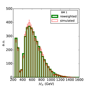
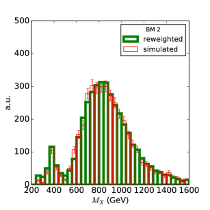
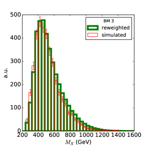
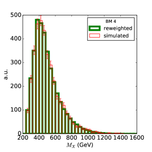
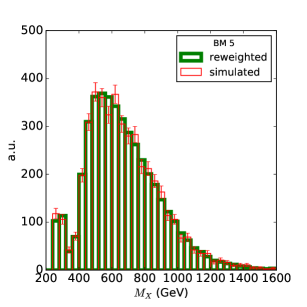
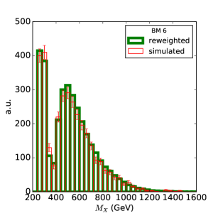
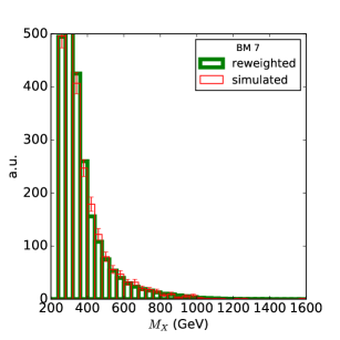
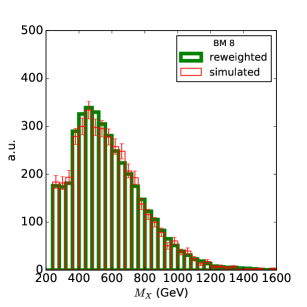
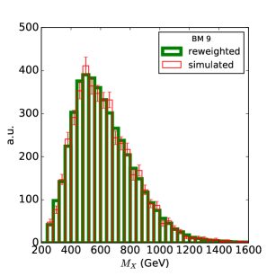
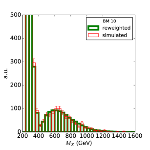
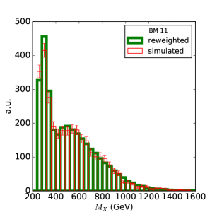
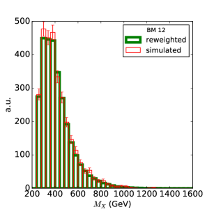
Figure 13: The reconstructed reduced mass after ATLAS-like selection. The histograms are normalized be signal efficiency times 100,000 events.

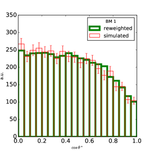
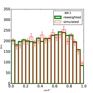
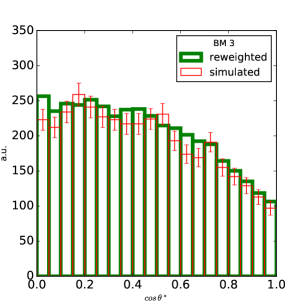
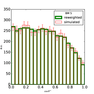
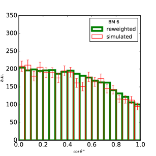
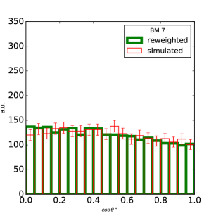
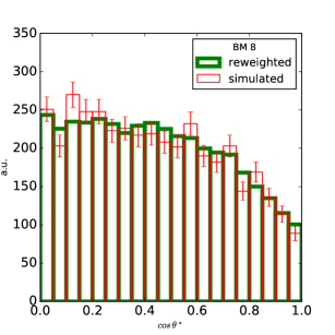
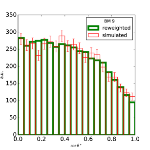
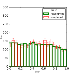
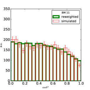
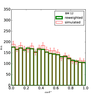
Figure 14: The reconstructed $\cos\theta^{*}$ after ATLAS-like selection. The histograms are normalized be signal efficiency times 100,000 events.

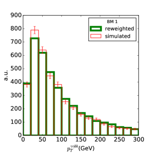
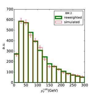
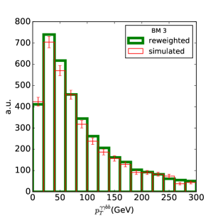
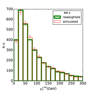
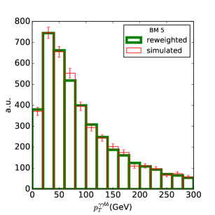
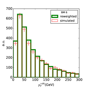
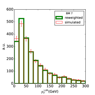
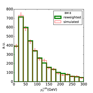
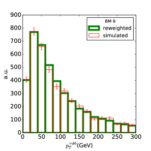
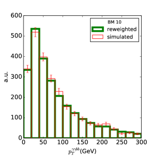
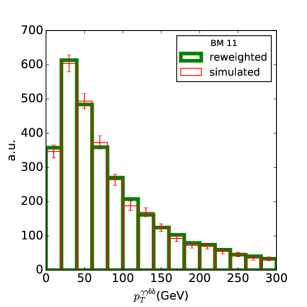
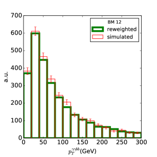
Figure 15: The reconstructed $p_{T}^{\gamma\gamma b\bar{b}}$ after ATLAS-like selection. The histograms are normalized be signal efficiency times 100,000 events.

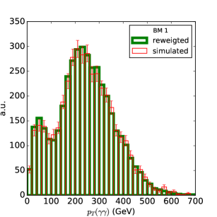
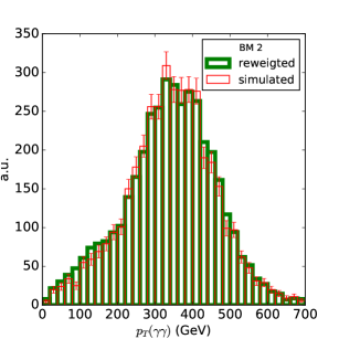
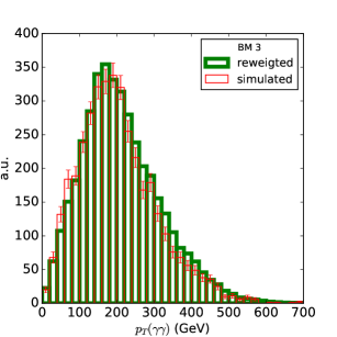
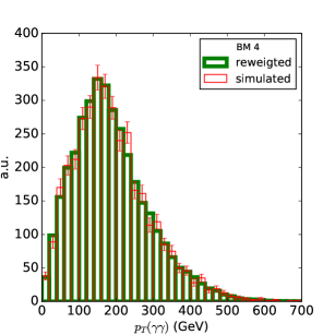
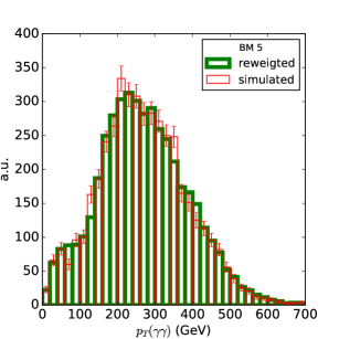
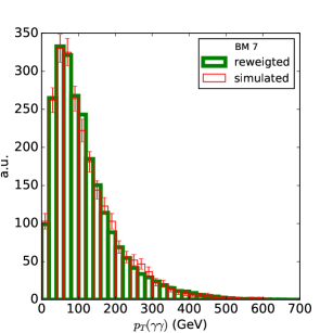
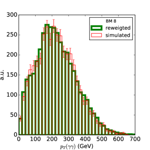
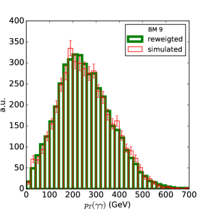
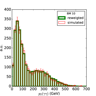
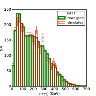
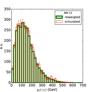
Figure 16: The reconstructed $p_{T}(\gamma\gamma)$ after ATLAS-like selection. The histograms are normalized be signal efficiency times 100,000 events.

References

- [1] I. V. Krive and Andrei D. Linde “On the Vacuum Stability Problem in Gauge Theories” In Nucl. Phys. B117, 1976, pp. 265–268 DOI: 10.1016/0550-3213(76)90573-3
- [2] Manfred Lindner, Marc Sher and Helmut W. Zaglauer “Probing Vacuum Stability Bounds at the Fermilab Collider” In Phys. Lett. B228, 1989, pp. 139–143 DOI: 10.1016/0370-2693(89)90540-6
- [3] Giuseppe Degrassi, Stefano Di Vita, Joan Elias-Miro, Jose R. Espinosa, Gian F. Giudice, Gino Isidori and Alessandro Strumia “Higgs mass and vacuum stability in the Standard Model at NNLO” In JHEP 08, 2012, pp. 098 DOI: 10.1007/JHEP08(2012)098
- [4] Christophe Grojean, Geraldine Servant and James D. Wells “First-order electroweak phase transition in the standard model with a low cutoff” In Phys. Rev. D71, 2005, pp. 036001 DOI: 10.1103/PhysRevD.71.036001
- [5] Florian Goertz “Electroweak Symmetry Breaking without the Term” In Phys. Rev. D94.1, 2016, pp. 015013 DOI: 10.1103/PhysRevD.94.015013
- [6] Peisi Huang, Aniket Joglekar, Bing Li and Carlos E. M. Wagner “Probing the Electroweak Phase Transition at the LHC” In Phys. Rev. D93.5, 2016, pp. 055049 DOI: 10.1103/PhysRevD.93.055049
- [7] G. F. Giudice, C. Grojean, A. Pomarol and R. Rattazzi “The Strongly-Interacting Light Higgs” In JHEP 06, 2007, pp. 045 DOI: 10.1088/1126-6708/2007/06/045
- [8] R. Grober and M. Muhlleitner “Composite Higgs Boson Pair Production at the LHC” In JHEP 06, 2011, pp. 020 DOI: 10.1007/JHEP06(2011)020
- [9] Adrian Carmona and Florian Goertz “A naturally light Higgs without light Top Partners” In JHEP 05, 2015, pp. 002 DOI: 10.1007/JHEP05(2015)002
- [10] Alexandra Carvalho, Martino Dall’Osso, Tommaso Dorigo, Florian Goertz, Carlo A. Gottardo and Mia Tosi “Higgs Pair Production: Choosing Benchmarks With Cluster Analysis” In JHEP 04, 2016, pp. 126 DOI: 10.1007/JHEP04(2016)126
- [11] Aleksandr Azatov, Roberto Contino, Giuliano Panico and Minho Son “Effective field theory analysis of double Higgs boson production via gluon fusion” In Phys. Rev. D92.3, 2015, pp. 035001 DOI: 10.1103/PhysRevD.92.035001
- [12] Florian Goertz, Andreas Papaefstathiou, Li Lin Yang and José Zurita “Higgs boson pair production in the D=6 extension of the SM” In JHEP 04, 2015, pp. 167 DOI: 10.1007/JHEP04(2015)167
- [13] Roberto Contino, Adam Falkowski, Florian Goertz, Christophe Grojean and Francesco Riva “On the Validity of the Effective Field Theory Approach to SM Precision Tests” In JHEP 07, 2016, pp. 144 DOI: 10.1007/JHEP07(2016)144
- [14] The ATLAS collaboration “Search for the Standard Model Higgs boson produced in association with a vector boson and decaying to a pair in collisions at 13 TeV using the ATLAS detector”, 2016
- [15] J. Alwall, R. Frederix, S. Frixione, V. Hirschi, F. Maltoni, O. Mattelaer, H. S. Shao, T. Stelzer, P. Torrielli and M. Zaro “The automated computation of tree-level and next-to-leading order differential cross sections, and their matching to parton shower simulations” In JHEP 07, 2014, pp. 079 DOI: 10.1007/JHEP07(2014)079
- [16] Neil D. Christensen, Priscila Aquino, Celine Degrande, Claude Duhr, Benjamin Fuks, Michel Herquet, Fabio Maltoni and Steffen Schumann “A Comprehensive approach to new physics simulations” In Eur. Phys. J. C71, 2011, pp. 1541 DOI: 10.1140/epjc/s10052-011-1541-5
- [17] Celine Degrande, Claude Duhr, Benjamin Fuks, David Grellscheid, Olivier Mattelaer and Thomas Reiter “UFO - The Universal FeynRules Output” In Comput. Phys. Commun. 183, 2012, pp. 1201–1214 DOI: 10.1016/j.cpc.2012.01.022
- [18] Benoit Hespel, David Lopez-Val and Eleni Vryonidou “Higgs pair production via gluon fusion in the Two-Higgs-Doublet Model” In JHEP 09, 2014, pp. 124 DOI: 10.1007/JHEP09(2014)124
- [19] “Search for Higgs boson pair production in the final state using pp collision data at TeV with the ATLAS detector”, 2016 URL: http://cds.cern.ch/record/2138949
- [20] “Search for decays at 13TeV”, 2016 URL: http://cds.cern.ch/record/2207960
- [21] Georges Aad “Searches for Higgs boson pair production in the channels with the ATLAS detector” In Phys. Rev. D92, 2015, pp. 092004 DOI: 10.1103/PhysRevD.92.092004
- [22] Georges Aad “Search For Higgs Boson Pair Production in the Final State using Collision Data at TeV from the ATLAS Detector” In Phys. Rev. Lett. 114, 2015 DOI: 10.1103/PhysRevLett.114.081802
- [23] Vardan Khachatryan “Search for two Higgs bosons in final states containing two photons and two bottom quarks in proton-proton collisions at 8 TeV” In Phys. Rev. D94, 2016 DOI: 10.1103/PhysRevD.94.052012
- [24] Albert M Sirunyan “Search for resonant and nonresonant Higgs boson pair production in the bblnulnu final state in proton-proton collisions at sqrt(s) = 13 TeV”, 2017 arXiv:1708.04188 [hep-ex]
- [25] Albert M Sirunyan “Search for Higgs boson pair production in events with two bottom quarks and two tau leptons in proton-proton collisions at sqrt(s) = 13 TeV”, 2017 arXiv:1707.02909 [hep-ex]
- [26] Alexandra Carvalho, Martino Dall’Osso, Pablo De Castro Manzano, Tommaso Dorigo, Florian Goertz, Maxime Gouzevich and Mia Tosi “Analytical parametrization and shape classification of anomalous HH production in the EFT approach”, 2016 arXiv:1608.06578 [hep-ph]
- [27] D. Florian “Handbook of LHC Higgs Cross Sections: 4. Deciphering the Nature of the Higgs Sector”, 2016 arXiv:1610.07922 [hep-ph]
- [28] Daniel Florian, Ignacio Fabre and Javier Mazzitelli “Higgs boson pair production at NNLO in QCD including dimension 6 operators”, 2017 arXiv:1704.05700 [hep-ph]
- [29] Jon Butterworth “PDF4LHC recommendations for LHC Run II” In J. Phys. G43, 2016 DOI: 10.1088/0954-3899/43/2/023001
- [30] Sayipjamal Dulat, Tie-Jiun Hou, Jun Gao, Marco Guzzi, Joey Huston, Pavel Nadolsky, Jon Pumplin, Carl Schmidt, Daniel Stump and C. P. Yuan “New parton distribution functions from a global analysis of quantum chromodynamics” In Phys. Rev. D93.3, 2016, pp. 033006 DOI: 10.1103/PhysRevD.93.033006
- [31] L. A. Harland-Lang, A. D. Martin, P. Motylinski and R. S. Thorne “Parton distributions in the LHC era: MMHT 2014 PDFs” In Eur. Phys. J. C75.5, 2015, pp. 204 DOI: 10.1140/epjc/s10052-015-3397-6
- [32] Richard D. Ball “Parton distributions for the LHC Run II” In JHEP 04, 2015, pp. 040 DOI: 10.1007/JHEP04(2015)040
- [33] Torbjörn Sjöstrand, Stefan Ask, Jesper R. Christiansen, Richard Corke, Nishita Desai, Philip Ilten, Stephen Mrenna, Stefan Prestel, Christine O. Rasmussen and Peter Z. Skands “An Introduction to PYTHIA 8.2” In Comput. Phys. Commun. 191, 2015, pp. 159–177 DOI: 10.1016/j.cpc.2015.01.024
- [34] J. Favereau, C. Delaere, P. Demin, A. Giammanco, V. Lemaître, A. Mertens and M. Selvaggi “DELPHES 3, A modular framework for fast simulation of a generic collider experiment” In JHEP 02, 2014, pp. 057 DOI: 10.1007/JHEP02(2014)057
- [35] Matteo Cacciari, Gavin P. Salam and Gregory Soyez “The anti-kt jet clustering algorithm” In JHEP 04, 2008, pp. 063 DOI: 10.1088/1126-6708/2008/04/063
- [36] “CMS Delphes card” Accessed: 2017-06-15, https://github.com/delphes/delphes/blob/master/cards/delphes_card_CMS.tcl
- [37] Sally Dawson and Christopher W. Murphy “Standard Model EFT and Extended Scalar Sectors”, 2017 arXiv:1704.07851 [hep-ph]
- [38] Jorge Blas, Mikael Chala, Manuel Perez-Victoria and Jose Santiago “Observable Effects of General New Scalar Particles” In JHEP 04, 2015, pp. 078 DOI: 10.1007/JHEP04(2015)078
- [39] Hermès Bélusca-Maïto, Adam Falkowski, Duarte Fontes, Jorge C. Romão and João P. Silva “Higgs EFT for 2HDM and beyond” In Eur. Phys. J. C77.3, 2017, pp. 176 DOI: 10.1140/epjc/s10052-017-4745-5
- [40] F. Aguila, M. Perez-Victoria and Jose Santiago “Observable contributions of new exotic quarks to quark mixing” In JHEP 09, 2000, pp. 011 DOI: 10.1088/1126-6708/2000/09/011
- [41] F. Aguila, J. Blas and M. Perez-Victoria “Effects of new leptons in Electroweak Precision Data” In Phys. Rev. D78, 2008, pp. 013010 DOI: 10.1103/PhysRevD.78.013010
- [42] Roberto Contino, Margherita Ghezzi, Christophe Grojean, Margarete Muhlleitner and Michael Spira “Effective Lagrangian for a light Higgs-like scalar” In JHEP 07, 2013, pp. 035 DOI: 10.1007/JHEP07(2013)035
- [43] Roberto Contino “The Higgs as a Composite Nambu-Goldstone Boson” In Physics of the large and the small, TASI 09, proceedings of the Theoretical Advanced Study Institute in Elementary Particle Physics, Boulder, Colorado, USA, 1-26 June 2009, 2011, pp. 235–306 DOI: 10.1142/9789814327183_0005
- [44] S. Baker and R. D. Cousins “Clarification of the Use of Chi Square and Likelihood Functions in Fits to Histograms” In Nucl. Instr. Meth., 1984, pp. 437–442
- [45] S.S. Wilks “The Large-Sample Distribution of the Likelihood Ratio for Testing Composite Hypotheses” In Annals Math.Statist. 9.1, 1938, pp. 60–62 DOI: 10.1214/aoms/1177732360
- [46] Fabio Maltoni, Eleni Vryonidou and Cen Zhang “Higgs production in association with a top-antitop pair in the Standard Model Effective Field Theory at NLO in QCD” In JHEP 10, 2016, pp. 123 DOI: 10.1007/JHEP10(2016)123
- [47] S. Dawson, A. Ismail and Ian Low “What’s in the loop? The anatomy of double Higgs production” In Phys. Rev. D91.11, 2015, pp. 115008 DOI: 10.1103/PhysRevD.91.115008
- [48] Giacomo Cacciapaglia, Haiying Cai, Alexandra Carvalho, Aldo Deandrea, Thomas Flacke, Benjamin Fuks, Devdatta Majumder and Hua-Sheng Shao “Probing vector-like quark models with Higgs-boson pair production” In JHEP 07.7, 2017, pp. 005 DOI: 10.1007/JHEP07(2017)005
- [49] Adam Falkowski, Benjamin Fuks, Kentarou Mawatari, Ken Mimasu, Francesco Riva and Verónica sanz “Rosetta: an operator basis translator for Standard Model effective field theory” In Eur. Phys. J. C75.12, 2015, pp. 583 DOI: 10.1140/epjc/s10052-015-3806-x
- [50] Roberto Contino, Margherita Ghezzi, Christophe Grojean, Margarete Mühlleitner and Michael Spira “eHDECAY: an Implementation of the Higgs Effective Lagrangian into HDECAY” In Comput. Phys. Commun. 185, 2014, pp. 3412–3423 DOI: 10.1016/j.cpc.2014.06.028
- [51] G. Brooijmans “Les Houches 2015: Physics at TeV colliders - new physics working group report” In 9th Les Houches Workshop on Physics at TeV Colliders (PhysTeV 2015) Les Houches, France, June 1-19, 2015, 2016 arXiv: https://inspirehep.net/record/1456803/files/arXiv:1605.02684.pdf