Toward the analysis of JWST exoplanet spectra:
Identifying troublesome model parameters

Abstract

Given the forthcoming launch of the James Webb Space Telescope (JWST) which will allow observing exoplanet atmospheres with unprecedented signal-over-noise ratio, spectral coverage and spatial resolution, the uncertainties in the atmosphere modelling used to interpret the data need to be assessed. As the first step, we compare three independent 1D radiative-convective models: ATMO, Exo-REM and petitCODE. We identify differences in physical and chemical processes taken into account thanks to a benchmark protocol we developed. We study the impact of these differences on the analysis of observable spectra. We show the importance of selecting carefully relevant molecular linelists to compute the atmospheric opacity. Indeed, differences between spectra calculated with Hitran and ExoMol exceed the expected uncertainties of future JWST observations. We also show the limitation in the precision of the models due to uncertainties on alkali and molecule lineshape, which induce spectral effects also larger than the expected JWST uncertainties. We compare two chemical models, Exo-REM and Venot Chemical Code, which do not lead to significant differences in the emission or transmission spectra. We discuss the observational consequences of using equilibrium or out-of- equilibrium chemistry and the major impact of phosphine, detectable with the JWST.Each of the models has benefited from the benchmarking activity and has been updated. The protocol developed in this paper and the online results can constitute a test case for other models.

1 Introduction

Since the publication of the detection of an extrasolar planet orbiting the 51 Peg star by Mayor & Queloz (1995), the field of exoplanet detection has developed very rapidly; more than 3700 exoplanets have been detected so far (e.g. exoplanet.eu). The field is now shifting more and more from the detection of exoplanets to the characterization of known exoplanets, especially their atmosphere, thanks to spectroscopic observations in the visible and infrared. One of the prime facilities used so far to observe the atmosphere of transiting exoplanets has been the Hubble Space Telescope (HST) (see the review by Deming & Seager, 2017, and references therein). Thanks to the use of the so-called scanning observing techniques with the WFC3 instrument, as well as sophisticated data reduction methods, variation of the star flux due to the transit of an exoplanet has been detected down to a few tens of ppm (Kreidberg et al., 2014; Tsiaras et al., 2016). In the near future, the James Webb Space Telescope (JWST, see jwst.stsci.edu), thanks to a large collecting area and a suite of state to the art instruments covering a large wavelength range (0.6-28 microns), will be a key machine to study the atmosphere of exoplanets (e.g. Greene et al., 2016; Mollière et al., 2017). The JWST will not only be used to study transiting/eclipsing exoplanets, but also exoplanets observed by direct imaging, thanks to its high angular resolution. For those exoplanets, far enough from the star to allow spectroscopic observations, spectra of exoplanet emission with a signal over noise ratio greater than 100 are expected.

Atmospheric models are needed to interpret the observations quantitatively. Several models have been developed over the years (for example see the reviews by Helling et al., 2008; Marley & Robinson, 2015; Hubeny, 2017, and the references there-in). Given the high observational precision achieved nowadays with current facilities and in the near future with the JWST, the question of comparing the uncertainties in the model predictions with the precision of the observations has to be considered. To tackle the question, we have, as a first step, only considered one dimensional models. To investigate the uncertainties in the models prediction, our approach has been to start with the comparison of the results from three models developed independently: the petitCODE model (Mollière et al., 2015, 2017), the ATMO model (Tremblin et al., 2015) and the Exo-REM model (Baudino et al., 2015). To identify the differences between the models and their impact on the predicted spectra, we have adopted a benchmark approach to give a common basis to the models allowing disentangling the impact of such or such differences.

In the second Section of the paper, the current version of the codes are briefly discussed and their differences outlined. The next section describes the protocol developed to benchmark the models. The results of the benchmark are discussed in Sect. 4. In Sect. 5, we focus on the evaluation of the uncertainties due to the ways the shape of resonant line far wings of alkalies are treated and due to the molecule far wing lineshape in use. In Sect. 6, we consider out-of-equilibrium chemistry (see Moses et al., 2011; Venot et al., 2012; Line & Yung, 2013; Zahnle & Marley, 2014; Hu et al., 2015) using two approaches coming from Exo-REM and Venot et al. (2012) and the observational consequences of this phenomenon. Then, in Sect. 7, we compare the deviation due to the different modelling approaches to the expected JWST uncertainties. The conclusions and perspectives are drawn in Sect. 8.

2 Description of the radiative-convective equilibrium models

Before focusing on the benchmark itself, we describe here the current state of the three radiative-convective equilibrium models which have been benchmarked. This is the state of the models taking into account the evolution resulting from the benchmark.

These models compute the 1D vertical structure of the atmosphere of giant planets and generate emission and/or transmission spectra given a set of input parameters: the effective temperature $T_{\mathrm{eff}}$, the surface gravity $\log_{10}(g)$, the radius and the elemental composition.

The atmosphere is discretised in a number of layers (50, 64 and 120 respectively for ATMO, Exo-REM and petitCODE). The models calculate the net energy flux as a function of pressure level using the radiative transfer equation, and solve it iteratively for radiative-convective equilibrium, i.e. conservation of the flux. The codes also incorporate a thermochemical model that calculates layer-by-layer the molecular mole fractions, given the elemental abundances and temperature profile. Heating sources, which can be internal (e.g. coming from the formation and evolution process) or external (e.g. coming from the star), are taken into account.

All the models take the internal heating due to the contraction of the planet into account:

• ATMO and petitCODE consider additional heating by the star radiation and are thus adapted to model close-in exoplanets and to calculate transit spectra.

• Exo-REM is only suited to young giant exoplanets for which stellar heating can be neglected with respect to the internal heat flux. This model is not able to compute transmission spectra.

One of the key drivers to determine the structure of an atmosphere is its opacity, which depends on its atomic and molecular composition, which, in turn, depends on the chemistry at work in the atmosphere.

2.1 Opacities

All the models consider continuum collisional induced absorption (CIA) for H₂–H₂ and H₂–He from the same references, atomic absorption coming from Na and K with various approaches for the resonant lines (see Sect. 5.1), molecular absorption coming from H₂O, CH₄, CO, CO₂, NH₃, PH₃, TiO, and VO. A lot of work has been recently devoted to update molecular linelists, especially by the Exomol team (see exomol.com). The references for the molecular linelists used in the various models are given in Table 1. It is interesting to note that, except for CO₂, at least two of the three models use the same linelist for a given molecule, which makes possible to infer the influence of using different linelists. Absorption coefficients are computed for a broadening due to:

• terrestrial atmosphere (air) for petitCODE

• a mix of H₂ and He for ATMO, Exo-REM.

Table 1: References of the different sources of molecular opacities for the three models considered here (ATMO, Exo-REM, petitCODE)

Opacities	Common references
CH4	Yurchenko & Tennyson (2014)
TiO and VO	Plez (1998) (with update from private communication)
H2–H2,	HITRAN (Richard et al., 2012)
H2–He	Borysow et al. (2001) and Borysow (2002)
Opacities	ATMO	Exo-REM	petitCODE
H2O	Barber et al. (2006)	Rothman et al. (2010)	Rothman et al. (2010)
CO	Rothman et al. (2010)	Rothman et al. (2010)	Rothman et al. (2010),Kurucz (1993)
CO2	Tashkun & Perevalov (2011)	Rothman et al. (2013)	Rothman et al. (2010)
NH3	Yurchenko et al. (2011)	Yurchenko et al. (2011)	Rothman et al. (2013)
PH3	Sousa-Silva et al. (2015)	Sousa-Silva et al. (2015)	Rothman et al. (2013)

Note that PH₃ and CO₂ have been added in Exo-REM since the first version described in Baudino et al. (2015).

After considering the linelists sources we focus on how each model computes the shape of the wings of each line (except for alkalies fully described in Section 5.1 because the different approaches for the wings treatment of the atomic lines used in the models induce significant differences in the model predictions). Our three codes use Voigt profile but with various ”cut-off” (or sub-Lorentzian lineshape) implementations:

• For ATMO, the line cut-off is described in detail in Amundsen et al. (2014). The cut-off distance is calculated on-the-fly by estimating when the line mass absorption coefficient has reached a critical value.

• For petitCODE and Exo-REM the applied sub-Lorenzian lineshape comes from Hartmann et al. (2002) for all molecules except for CO₂ for which a profile from Burch et al. (1969) is used (see Mollière et al., 2017).

For fast computation, the opacity is treated by using opacity distribution functions and making use of the correlated-k assumption. This technique is very useful, especially to manage the large number of lines in modern molecular linelists. In our case, all models use correlated-k coefficients computed molecule-by-molecule.

Our three models combine the molecules assuming no correlation between species in any spectral interval. This is done using the method named ”reblocking of the joint k–distribution” by Lacis & Oinas (1991) and more extensively described in Mollière et al. (2015) (”R1000” method in their Appendix B.2.1) with a few differences for ATMO as described in Amundsen et al. (2014, 2016).

2.2 Equilibrium chemistry

The three models compute the equilibrium chemistry using various methods.

ATMO and petitCODE use a Gibbs energy minimisation scheme following the method of Gordon & McBride (1994).

ATMO uses the same thermochemical data as Venot et al. (2012) in the form of NASA polynomial coefficients (see McBride et al., 1993). The Gibbs minimizing method allows for depletion of gas phase species due to condensation and is included in the chemical solver.

petitCODE uses the same NASA polynomials, but extends them to the low temperatures ($<$200 K) using the JANAF database (see also Appendix A2 of Mollière et al., 2017).

Exo-REM solves the thermochemical equilibrium layer-by-layer using on-line JANAF data from Chase (1998). Exo-REM does not use a general Gibbs energy minimisation scheme, but a simplified approach. The molecules are grouped by independent sub-sets (see Tab. 2 in Baudino et al., 2015). In a given sub-set, the molecular mole fractions are found by solving a system of equations consisting of equilibrium constants and element conservation. When condensation occurs in a layer, the elements trapped in the condensed species are considered as lost for the chemistry occuring at higher layers. Doing so, ExoREM includes the so-called cold trap phenomenon in contrast to ATMO and petitCODE.

3 Benchmark protocol

The two following sections (Sect. 3 and 4) are focused on the benchmark itself. First, we define a ”common” model to compare the results of our models (Sect. 3.1) and the test protocol used to obtain the results (Sect. 3.2 and 3.3). Then we compare the results of this benchmark in Sect. 4.

3.1 Definition of a ”common” model

The starting point of a benchmark is the definition of a common set of parameters and of physical, chemical processes to be taken into account. Given that one of the key parameters determining the vertical structure of an atmosphere is its atmosphere composition, we have first to define a common set of absorbers.

The common model considers the opacities from the most important molecules and atoms: NH₃, CH₄, CO, CO₂, H₂O, PH₃, Na, K, as well as the collision-induced absorption for H₂–H₂ and H₂–He. For the alkalies we use the following H₂ broadening coefficients:

• Na: $0.37\times(T/296)^{-0.65}$cm^-1atm^-1 fitted to Allard et al. (2012),

• K: $0.40\times(T/296)^{-0.64}$cm^-1atm^-1 fitted toAllard et al. (2016).

For the far wings we use a Voigt profile up to 4500 cm^-1 from line center for all Na and K lines and zero absorption beyond. Other line shapes used in the literature are explored in sect. 5.1.TiO and VO are not taken into-account to keep a minimal ”common” model; we consider them only in the case of an extremely hot atmosphere. We have not considered the presence of clouds.

The abundance of the various absorbers depends on the chemical reactions at work in the atmosphere; we have considered a chemistry including the following reactant species: H₂, H, He, H₂O, H₂O(s), CO, CO₂, CH₄, NH₃, N₂, Na₂S(s), H₂S, Na, HCl, NaCl, K, KCl, KCl(s), NH₄Cl(s), SiO(s), Mg, Mg₂SiO₄(s), MgSiO₃(s), SiO₂(s), Fe, Fe(l), PH₃, H₃PO₄(l), P, P₂, PH₂, CH₃, SiH₄, PO.

Unless specified otherwise, we consider an atmosphere with a solar metallicity. We use solar elemental abundances from Asplund et al. (2009).

By default, the radius, at 10 bars, of the exoplanet is fixed at 1.25 $R_{\mathrm{jup}}$ (where $R_{\mathrm{jup}}$ is the radius of Jupiter; we use 69911 km for 1 $R_{\mathrm{jup}}$) and the distance between the exoplanet and the observer is fixed at 10 pc.

After adapting (upgrading or downgrading) our models to this common model, we generated spectra and atmospheric structures (composition and temperature) in the following conditions.

3.2 Comparison with fixed temperature profiles

First, we compute the abundance profiles at chemical equilibrium and spectra for five given temperature profiles. Indeed our models are such that it is possible to impose a pressure–temperature profile (PT profile), and then run them without reaching the radiative-convective equilibrium, by just computing the chemistry and doing the radiative transfer only. We compare the result without iteration of the models in exactly the same conditions (in Sect. 3.3 we apply the iterations needed for the full convergence of a model to radiative-convective equilibrium).

Figure 1: Input pressure-temperature profiles used in the benchmark

We use the thermal profiles of Guillot (2010) (Fig. 1), with surface gravity $\log_{10}(g[\mathrm{cgs}])$=3.7, solar metallicites and effective temperatures (corresponding to the model of Guillot, these T_eff are not necessary consistent with models used here) of: 500 K, 1000 K, 1500 K, 2000 K, and 2500 K. More specifically, we use Equation (29) of Guillot (2010), with f = 1/4, $\gamma=0.4$, $\kappa=0.01$ and $T_{\rm int}=200$ K. For T_eff = 1000 K, we use two additional values of the metallicity: 3 and 30 times the solar value.

This allows us to explore how our results compare for a broad range of temperatures, as well as different enrichment values.

3.3 Comparison of self-consistent calculations

As a next step we compare self-consistent atmospheric solutions of our codes, calculating radiative-convective equilibrium structures for known exoplanets. In the previous section, we fixed the same temperature-profile in each model, while in this section, we impose the $T_{\mathrm{eff}}$ itself. It means that we have to iterate on the P-T profile to get a self-consistent solution to the transfer equation. We do this for two direct imaging and two transiting exoplanets. We run our models, considering published physical parameters for the exoplanets (based on http://exoplanet.eu).

For the two self-luminous planets we stay in the benchmark condition, except for the metallicity. GJ 504 b (Kuzuhara et al., 2013) is a cold planet with $T_{\mathrm{eff}}$=510 K, $\log(g)$=3.9 and a metallicity z=0.28 dex. VHS 1256–1257 b (Gauza et al., 2015) is an object hotter than GJ 504 b with $T_{\mathrm{eff}}$=880 K, $\log(g)$=4.24 and a metallicity z=0.21 dex. In the absence of strong constraints on the radius, we keep the benchmark value of 1.25 $R_{\mathrm{Jup}}$.

For the two irradiated transiting exoplanets we keep the solar metallicity but adapt the radius to the published values. For GJ 436 b (Butler et al., 2004), the host star parameters are: an effective temperature $T_{\mathrm{eff}}$ of 3684 K and a radius of 0.464 solar. The planet has a $T_{\mathrm{eff}}$=712 K, a radius of 0.38 $R_{\mathrm{Jup}}$ and a mass of 0.07 $M_{\mathrm{Jup}}$. The incidence angle of the irradiation $\cos(\theta)$=0.5. The irradiation of the second transiting exoplanet considered here, WASP 12 b (Hebb et al., 2009), is more extreme, and could possibly lead to a temperature inversion at high altitude. Thus for this planet, we decided to add the chemistry and opacities for TiO and VO. The host star parameters in this case are: an effective temperature $T_{\mathrm{eff}}$ of 6300 K and a radius of 1.599 solar. The planet has an high $T_{\mathrm{eff}}$=2536 K, a radius of 1.736 $R_{\mathrm{Jup}}$ and a mass of 1.04 $M_{\mathrm{Jup}}$. We assume an incidence angle for the irradiation of $\cos(\theta)$=0.5. For the Ti and V chemistry we considered Ti, TiO, V and VO.

4 Results

4.1 Results comparison

In this section, we present the results of the comparison between our models following the benchmark protocol. We show here a selection of plots to illustrate these results. In Appendix A, we attached the complete set of spectra and profiles for all the various test cases. All the data are available online (as supplementary material).

For each model, we compare the spectra, the abundance profiles of the absorbers and when relevant, i.e. for the four targets modelled in a self-consistent way, the temperature profiles. All spectra are plotted at the same spectral resolution (corresponding to that of Exo-REM, i.e. with a step and resolution of 20 cm^-1). The spectra are shown from near to mid-infrared, the wavelength range of the JWST.

Figure 2: Emission (a) and transmission (b) spectra for models at 1000 K with solar metallicity (solid), and 1000 K with $30\times solar$ metallicity (dashed)

Figure 3: Emission spectra (bottom to top) for effective temperatures of 1500, 2000, 2500 K

Figure 4: Emission spectra of VHS 1256-1257 b (top) and GJ 504 b (bottom). The black uncertainties correspond to the combination of simulated NIRSpec/Prism and MIRI/LRS noise level for VHS 1256-1257 b for 0.5 hour of integration.

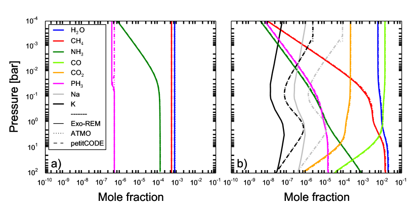
Figure 5: Abundance profiles of the defined molecules for the case with a T_eff =500 K at solar metallicity (a) and 1000 K at 30 $\times$ solar metallicity (b). The curves for the models are often superposed, except for alkalies where Exo-REM is not.

At the end of our convergence process (fully described in Section 4.2), we reached a good agreement between all models in the common model conditions. This is observable in Fig. 2, which shows the spectra of the cases with a T_eff = 1000 K at solar and super-solar metallicities. Figure 3 shows the spectra for the three hottest cases (T_eff = 1500 K, 2000 K, 2500 K) with also good agreement between ATMO, petitCODE and Exo-REM. If we consider the general trend, the emission, transmission spectra and molecular abundances calculated by the three radiative-convective equilibrium models are very similar. It is especially interesting to see how similar spectra of exoplanet targets are without pre-defined temperature profile in the models (Fig. 4, and in Appendix A Fig. 25).

Nonetheless, we still observe some differences and we will be focusing on these in the following paragraphs.

To highlight the impact of the remaining differences, we investigate the predicted error bars from JWST observations for VHS 1256–1257 b in Fig. 4.

To obtain these error bars, we use the JWST Estimator Time Calculator (https://jwst.etc.stsci.edu/) to simulate a half an hour observation with the NIRSpec JWST instrument using the prism mode and with the MIRI JWST instruments using the Low Resolution Spectroscopic mode.

While ATMO and Exo-REM codes provide similar results within the error bars, petitCODE provides results significantly different. In the case of Fig. 4 its comes mainly from linelists differences as present in the next section.

4.1.1 Differences due to opacities

A large part of the differences originates from the absorption of PH₃, more observable for low temperature cases (4-5 $\mu$m, Fig. 4 and in Appendix A Figs. 21 a, b, 25 a and b), which is treated differently, depending on the code: petitCODE uses the linelist from HITRAN (Rothman & Gordon, 2013), while ATMO and Exo-REM use data from Exomol (Yurchenko & Tennyson, 2014).

There are also some differences between spectra (Fig. 2 ) at $\sim$ 6 $\mu$m and 10 $\mu$m (and, in Appendix A, Figs. 25 a and b) which are attributed to the use of different NH₃ linelists : petitCODE uses HITRAN, whereas the other codes use Exomol (Yurchenko et al., 2011). The use of only the main CO isotopologue buy petitCODE is at the origin of the differences observed between 4 and 5 microns in the high temperature cases (Fig. 4 and, in Appendix A, Figs. 23 b and c, 25 c).

The use of different linelists also affects the integral flux of the spectrum, i.e. the effective temperature (e.g., in Appendix A, the temperature profiles of the two self-luminous exoplanets, Fig. 27, are a bit shifted toward lower temperature for petitCODE, to compensate the lack of absorption).

These results point out the importance of updating line lists in the models in the JWST era.

At 2000 K and much more at 2500 K (Fig. 3 and, in Appendix A, Fig. 23 c), Exo-REM has more flux than the other models. The reason for this is the range of validity of this model. Not designed for irradiated objects, correlated-k coefficients of Exo-REM are not computed for high temperature / low pressure. A temperature higher than 1800 K, at high altitude (for a pressure $<$ 10^-5 bar), is out of the range of validity of Exo-REM.

Note that, we do not find differences coming from the fact that petitCODE uses air broadening, or from the correlated-k approaches of ATMO.

4.1.2 Differences due to chemistry

While there is no large difference in the spectra, large differences in some molecule and atom abundances can be observed (See Fig. 5), especially for PH₃ up to 0.1 bar for the case at 500 K (Fig. 5 a, and in Appendix A Figs. 26 a and b), and for the alkali in general at 1000 K (Fig. 5 b for 30 solar metallicity, and, in Appendix A Figs. 22 b, c, and d). These differences occur each time the condensation curve of a compound is crossed, and Exo-REM gives systematically lower abundances values. This effect is explained by the implementation of the cold trap in Exo-REM. Indeed, Exo-REM makes the following assumption: if a molecule condensates at a given level in the atmosphere, the material is lost for the upper layers. For instance, as alkali condensation occurs deep in the atmosphere, Exo-REM predicts a lower amount of Na and K than ATMO and petitCODE. These differences do not have a significant effect on spectra (Fig. 2).

4.2 Convergence process step-by-step

To arrive at the level of similarity presented in the previous section we had to make several changes in our models. In this section, we describe how we updated our models and the benchmark protocol.

Before the beginning of the benchmark, Exo-REM was updated by adding CO₂ to the absorbing molecules list and by updating the H₂–He CIA sources. Exo-REM also implemented a new way to combine correlated-k coefficients (described in Appendix B).

When we began this benchmark, we identified a major difference between the models concerning how the alkali far wings were accounted for (see Sect. 5.1). Without any good answer to this question (see Sect. 5.1), we decided to consider the same simple alkali treatment (same Voigt profiles with cut-off).

The other major difference was identified as coming from the molecular far wing lineshape. In fact, petitCODE did not initially include any cut-off in the line profile (unlike ATMO and Exo-REM). Across the full considered wavelength range, all lines had a Voigt profile (see Mollière et al., 2015, Appendix A for the scheme). The first consequence of this comparison is that petitCODE now also includes a line cut-off as its default line opacity treatment, implemented in the same way as in Exo-REM. Moreover, we study the effect of considering a cut-off, when compared to the case without any cut-off application, in Section 5.2.

These modifications lead to a significant improvement of the convergence. Then, we spotted a strong absorption in petitCODE results (between 4 and 5 $\mu$m), not visible in the results from other models. The corresponding absorber was PH₃, not added at this stage neither in ATMO nor Exo-REM. This implied an important modification of ATMO and Exo-REM to add the chemistry and absorption of phosphine. This molecule has now been included in these models.

At this step, spectra obtained with the three models began to show good agreements, but we still observed differences that were identified as due to methane features and to H₂-He CIA. These differences came from the use of different CH₄ line lists and continuum collisional-induced absorption coefficients. Indeed at that time petitCODE did not use the latest version of CH₄ linelist but used that of Rothman et al. (2013); it also was not using the latest CIA values but those of Borysow et al. (2001); Borysow (2002). ATMO used an updated version of H₂-He CIA (Richard et al., 2012) but not a complete one compare to Exo-REM (see Appendix B). Once each model used the CH₄ lines list, and the same H₂-He CIA as Exo-REM, the differences disappeared.

Three other effects have been identified as being important to converge on the results.

In the extreme case with a T_eff= 2500 K petitCODE showed a strong effect due to ionization, a process not taken into account by the other models; hence we decided to deactivate it for the benchmark protocol.

The next two effects have an impact on transmission spectra and were observable only at the end of the whole convergence process. They are taken into account to achieve the remarkably similar spectra that we obtained for the self-consistent transiting targets WASP 12 b and GJ 436 b (see in Appendix A Fig. 25 c).

First, the mean molecular weight (MMW) is known to have a strong effect on transmission spectra (Miller-Ricci et al., 2009; Croll et al., 2011). In the beginning of the benchmark study, the chemistry code written for and used for the first time in petitCODE (Mollière et al., 2017), erroneously included condensate species for calculating the MMW, for which the condensate mass fraction and condensate monomer mass was used. This mistake was spotted quickly during our benchmark process, and corrected before the publication of Mollière et al. (2017), and therefore never affected any published results and models of petitCODE.

The reason for the difference to occur is that the monomers can be significantly more massive than the gas species molecules from which they are constructed, e.g. for silicates such as Mg₂SiO₄, leading to an overestimation of the MMW, which resulted in noticeable differences in the output transmission spectra between ATMO and petitCODE. In reality, condensible species only affect the MMW by depleting heavier molecules and atoms from the gas phase, hence leading to a decrease in MMW, rather than an increase. As the condensate particles in the atmosphere, which have masses much larger than the monomer mass, will usually not be sufficiently well collisionally coupled to the atmospheric gas, they should not be taken into account in the calculation of the MMW.

Second, transit spectroscopy is also sensitive to the pressure-radius profile used. It appears that we need to have exactly the same radius at a pressure of 10 bars to obtain similar transmission spectra without an offset.

5 Focus on key parameters effects

During the benchmark we realized that the uncertainties in two inputs of the models, i.e. the alkali line profiles, and the molecules far line-wing shape, lead to significant uncertainties in the results. In this section we detail the effects of these uncertainties.

5.1 Alkali line profiles

At temperatures below the condensation of TiO/VO ($<$2000 K), the opacity in the visible part of the spectrum is dominated by the wings of the Na-D (5890 Å) and KI (7700 Å) resonance lines. While an accurate treatment of the line shape of usual atomic lines is only needed at $\sim$ 25 Å from the line center, the alkali resonant lines far wings profile at thousands of Ångström from the line center still induce an important absorption effect. In the past literature from brown dwarfs atmosphere modelling, two groups have tried to address the issue of the shape of the alkali-resonant-line far wings:

• Burrows & Volobuyev (2003) have used standard quantum chemical codes and the unified Franck-Condon model in the quasi-static limit to calculate the interaction potentials and the wing shapes for the alkali resonant lines in H₂/He atmospheres.

• Allard et al. (2007) have used a unified line shape semi- classical theory (Allard et al., 1999) using molecular potentials computed using a valence pseudo-potential (see Allard et al., 2007).

To our knowledge, these two works have never been benchmarked in the astrophysics literature. In this section, we illustrate the effects of the different alkali treatments by using the ATMO code on the Guillot–1500K equilibrium PT profile, and on the radiative/convective solution for GJ 504 b. We have used three treatments:

• The Voigt profiles as defined in Sect. 3.1

• The ”Burrows” profiles as implemented by Baudino et al. (2015)

• The ”Allard” profiles as used in Tremblin et al. (2015)

5.1.1 Guillot profile T_eff = 1500 K

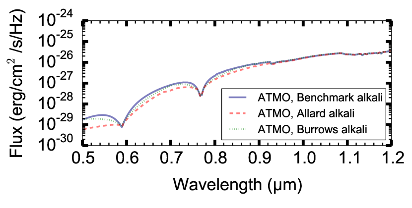
Figure 6: Effects of the different alkali treatments on the emission spectra for the Guillot profile with $T_{\mathrm{eff}}$=1500K.

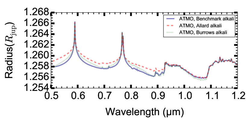
Figure 7: Effects of the different alkali treatments on the transmission spectra for the Guillot profile with $T_{\mathrm{eff}}$=1500K.

We first perform a benchmark study on a fixed PT profile, the Guillot T_eff=1500 K profile used in Sect. 2.1. Figures 6 and 7 show the emission and transmission spectra. Both spectra highlight a low absorption in the wings of the Voigt profile; both Burrows and Allard profiles increase the absorption in the far wings. Yet, this increase is significantly bigger with the Allard profile and the use of one or the other is therefore not neutral. For a Jupiter like exoplanet transiting a solar type star, the difference between the transmission spectrum using Allard profiles or Burrow profiles is found to be in the 20 ppm range, which is accessible to observations with the JWST. But these differences should be attenuated when using models with clouds, so that it might be difficult to disentangle which profile fits better the observations.

5.1.2 GJ504b

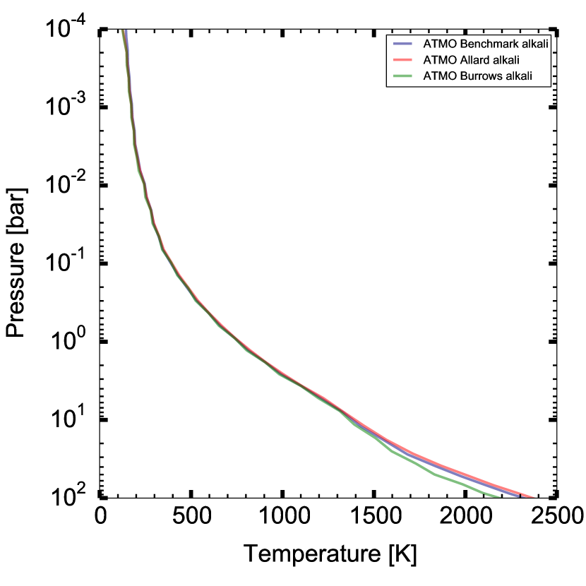
Figure 8: Effects of the different alkali treatments on the PT profiles computed in radiative/convective equilibrium for GJ504b.

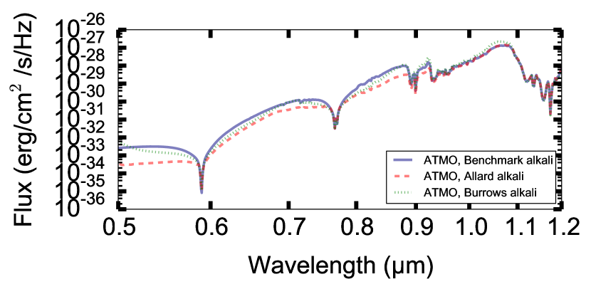
Figure 9: Effects of the different alkali treatments on the emission spectrum of GJ504b.

We have used the different alkali treatments in the radiative/convective equilibrium model for GJ 504 b. Figure 8 shows the effects on the converged PT profile, the Allard profile leads to a slightly warmer deep atmosphere than the Voigt profile and the Burrows profile to a significantly cooler deep atmosphere, with a difference of 100-200 K at 100 bars. These effects are directly linked to the differences in absorption caused by the line profile. Figure 9 shows the effects of the different alkali treatments on the emission spectrum of GJ 504 b.

The Allard profile leads to a higher absorption both below 0.9 $\mu$m and above 1 $\mu$m, compared to a simple Voigt profile. The Burrows profile leads to a higher absorption, compared to Voigt profile, below 0.9 $\mu$m but a lower one above 1 $\mu$m. In fact with the Burrows profile, there is no absorption caused by the potassium far wing in the Y band while a strong absorption is appearing with the Allard profile.

Comparisons with observations as done in Tremblin et al. (2015) for T dwarfs would favour the Burrows profile for this kind of object. The authors have used the Allard profile but they had to assume a condensation of potassium in KAlSi₃O₈ to remove all effects of the far wing on the Y band. We emphasize again that this conclusion depends on the model used to produce the NIR reddening (temperature gradient reduction in the case of Tremblin et al. 2015). In the other way, a comparison of the profile effects on the spectra of L dwarfs seems to favour the Allard profile (private communication B. Burmingham). The limits we have faced in this alkali-treatment benchmark strongly advocate for a community effort to have a better understanding on the far-wing behaviour as a function of pressure and temperature. It is also of great importance to get better constraints on the different cloud models or alternatives.

5.2 Molecular far wing lineshape

In this section we estimate the effect of applying a line ”cut-off” (a sub-Lorentzian far wing profile) in the Voigt profile of the molecular lines as described in Sect. 3. For that we compare to a Voigt profile without cut-off hereafter. Doing so, we face a difficulty with CH₄. Indeed the huge number of CH₄ lines made the calculation of CH₄ opacities without line cut-off infeasible (for this paper). To deal with that difficulty, we have estimated the effect of no cut-off in two ways: 1) first by considering the effect only on a limited wavelength range and with a fixed P-T profile (Sec. 5.2.1), and then by taking into account no cut off on all molecules, but CH₄, whose opacity is not considered, and doing a self-consistent calculation.

5.2.1 Comparison at fixed temperature structure

As a first step, we compare the results from a self-consistent atmospheric calculation for GJ 504 b as obtained by petitCODE including the sub-Lorentzian lineshape (cut-off), to those with full Voigt profiles, using the same temperature structure, however. We use the same set of absorbing species as in the baseline case. Due to the extensive line list of CH₄ (Yurchenko & Tennyson, 2014) we calculated the opacity for this molecule in the full Voigt case only within 1.1 to 1.4 $\mu$m, and neglected all lines outside of this spectral region. Therefore we will concentrate on this spectral region for our comparison. This spectral interval was chosen because both water and methane have an opacity minimum ranging from 1.2 to 1.3 $\mu$m, and a change in the line wing continuum should be most noticeable in such regions.

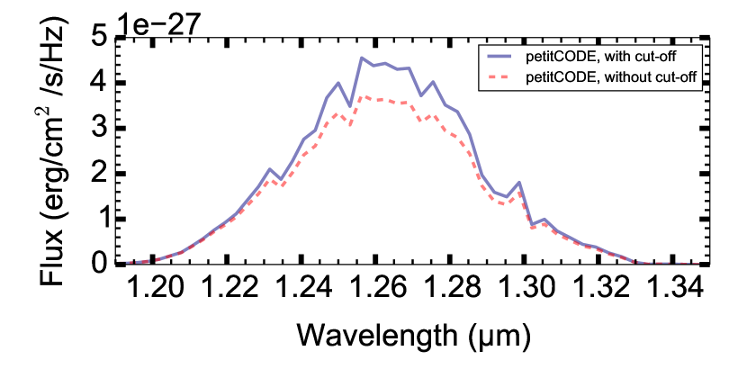
Figure 10: Emission spectra for GJ 504 b calculated using the nominal temperature structure of the case including sub-Lorentzian far wings. We show the resulting spectrum of the nominal case (blue solid line) as well as the case with full Voigt profiles (red dashed line).

The resulting emission spectra can be seen in Figure 10. The difference between the two cases is strongest in the peak of emission, i.e. in the location where the total line opacity was the smallest and the contribution of the line wing continuum the largest. We find maximum differences in the flux of the order of $\sim 20$ %. If we had included methane lines outside of the 1.1 to 1.4 $\mu$m region the decrease in emission may have been even stronger, with lines further away potentially still non-negligibly contributing to the line wing continuum.

5.2.2 Comparison for self-consistent structures

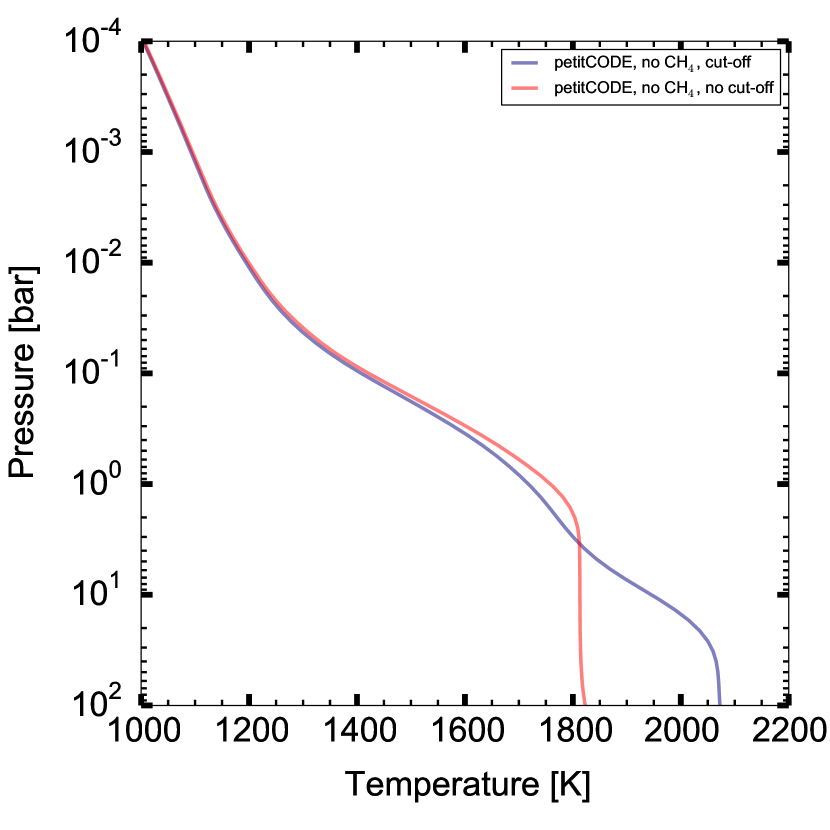
Figure 11: Pressure-temperature structures of the self-consistent hot Jupiter cases sub-Lorentzian and Lorentzian far wings, neglecting the methane opacity.

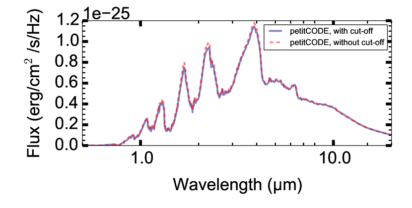
Figure 12: Emission spectra of the self-consistent hot Jupiter cases sub-Lorentzian and Lorentzian far wings, neglecting the methane opacity.

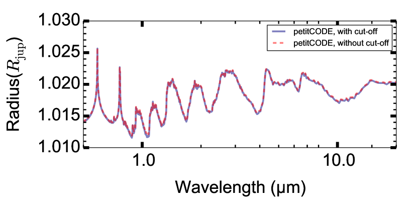
Figure 13: Transmission spectra of the self-consistent hot Jupiter cases sub-Lorentzian and Lorentzian far wings, neglecting the methane opacity.

The spectral test we carried out in the previous section was done only within a small spectral window, due to the extensive CH₄ line list, which makes the calculation of opacities applying a Lorentzian lineshape over the full spectral range infeasible and did not allow for comparing self-consistent structures and spectra arising from the Lorentzian vs. sub-Lorentzian lineshape calculations. In this section we therefore vary our baseline model and calculate hot Jupiter atmospheric structures without considering CH₄ opacities, because for all other species an opacity calculation with full Lorentzian lineshape is possible. We do not claim that an exclusion of CH₄ is realistic, although CH₄ should not be dominant at the elevated temperatures studied here, we merely carry out this test to study the effect of a line wing cut-off. The hot Jupiter is defined as an irradiated planet around a Sun- like star, with $T_{\rm eff}=1500$ K, $M_{\rm Pl}=1.2\ {\rm M}_{\rm Jup}$, $R_{\rm Pl}=1\ {\rm R}_{\rm Jup}$ (at 10 bar) and $T_{\rm int}=100$ K and an atmospheric enrichment of 3 times solar.

The $P$-$T$ structures, emission and transmission spectra of the self–consistent hot Jupiter cases with sub-Lorentzian and Lorentzian far wing, and neglecting the methane opacity, are shown in Figs. 11, 12, 13.

It can immediately be seen that the deep isothermal region of the full Voigt atmosphere is cooler, although the total opacity there is higher: The opacity increase arising from pure Voigt profiles causes the stellar light to be absorbed already at higher layers, leading to a small temperature increase between 0.1 and 3 bar in this atmosphere. Consequently, less flux has to be emitted from the optically thick, deeper regions of the planet, leading to a cooler temperature structure for pressures larger than 3 bar. Thus, in the presence of irradiation, the calculated temperature structure of an atmosphere can change significantly, depending on whether or not a Lorentzian lineshape is applied.

Because the higher regions of the atmosphere are not so strongly affected by the line far wings the flux changes in the absorption features of the emission spectra are small. The emission peaks, with radiation originating in the deeper and hotter regions of the atmosphere are affected more strongly, with maximum differences of 7 %, e.g. at 2.25 $\mu$m.

Over a wide wavelength range the differences between the two cases in the transmission spectrum are small, due to the fact that the transmission probes high layers of the atmosphere where (i) the temperature of the two cases is very similar and (ii) pressure broadening is less important. However, the largest differences in the optical and NIR, again at locations of minimum opacity, can be as large as $\sim 10$ % of the transmission signal amplitude (e.g. Y-band in Fig. 13). Such differences are greater than the expected precision of JWST observations of hot Jupiter around bright stars.

6 Non-equilibrium chemistry

6.1 Impact of non-equilibrium chemistry

Known since the 70’s in the atmospheres of the giant planets of our Solar System (Prinn & Barshay, 1977), non–equilibrium chemistry was discovered in a cool brown dwarf, Gl 229 b, in 1997 by Noll et al. (1997). More recently, it started to be considered for transiting exoplanets (e.g. Moses et al., 2011; Line & Yung, 2013) and evidence for non–equilibrium chemistry was also found in extrasolar directly imaged planets of the HR 8799 system (e. g. Barman et al., 2011, 2015; Konopacky et al., 2013) through the concomitant detection of CO absorption features and the unexpectedly weak absorption by CH₄.

This important phenomenon, which can strongly affect the atmospheric chemical composition, is due to a competition between vertical mixing and chemical kinetics. When the dynamical timescale is shorter than the chemical timescale we observe a freezing of the abundance of some species. The ”quenched” species keep the same abundances than that of the deep hot layers, where chemical equilibrium is achieved. This phenomenon, called transport–induced quenching, affects particularly the CO/CH₄ and N₂/NH₃ ratios that can be driven away from what is expected from equilibrium chemistry. For the atmospheres highly affected by quenching, the interpretation of observational spectra can thus be quite difficult.

6.2 Description of the chemicals models

To model the non-equilibrium chemistry that takes place in warm exoplanet atmospheres, two different approaches can be used: a complete modelling of kinetics with a model accounting for atmospheric mixing (like in Venot chemical model, Venot et al., 2012, hereafter V12), or a chemical equilibrium model coupled to a parametrization of the quenching level for the main species (like in Exo-REM).

Venot chemical model
The thermo–photochemical model developed by V12 is a full 1D time-dependent model. It includes kinetics, photodissociation and vertical mixing (eddy diffusion and molecular diffusion). To determine the atmospheric composition of a planet, the thermal profile is divided in discrete layers ($\sim$100) of thickness equal to a fixed fraction of the pressure scale height. The code solves the continuity equation (Eq. 1) for each species and for each atmospheric layer, until a steady-state is reached.

$$\frac{\partial n_{i}}{\partial t}=P_{i}-n_{i}L_{i}-div({\Phi_{i}}\overrightarrow{e_{z}})$$ (1)

where $n_{i}$ the number density of the species $i$ ($\mathrm{cm^{-3}}$), $P_{i}$ its production rate ($\mathrm{cm^{-3}\leavevmode\nobreak\ s^{-1}}$), $L_{i}$ its loss rate ($\mathrm{s^{-1}}$), and $\Phi_{i}$ its vertical flux ($\mathrm{cm^{-2}\leavevmode\nobreak\ s^{-1}}$) that follows the diffusion equation,

$$\Phi_{i}=-n_{i}D_{i}\left[\frac{1}{n_{i}}\frac{\partial n_{i}}{\partial z}+\frac{1}{H_{i}}+\frac{1}{T}\frac{dT}{dz}\right]-n_{i}K_{\mathrm{zz}}\left[\frac{1}{y_{i}}\frac{\partial y_{i}}{\partial z}\right],$$ (2)

where $y_{i}$ is the mixing ratio, $K_{\mathrm{zz}}$ is the eddy diffusion coefficient ($\mathrm{cm^{2}\leavevmode\nobreak\ s^{-1}}$), $D_{i}$ is the molecular diffusion coefficient ($\mathrm{cm^{2}\leavevmode\nobreak\ s^{-1}}$), and $H_{i}$ the scale height of the species $i$.

At both upper and lower boundaries, we impose a zero flux for each species.

The strength of this model relies on the chemical scheme it uses: the C₀–C₂ scheme. It describes the kinetics of 105 species made of H, C, O, and N, which are linked by $\sim$2000 reactions. This scheme has been implemented in close collaboration with specialists of combustion and has been validated experimentally as a whole (not only each reaction individually). The completeness of this scheme (both the forward and the reverse directions of each reaction are considered) implies that thermochemical equilibrium is achieved kinetically, or, conversely, that out of equilibrium processes are considered. The temperatures found in warm exoplanet atmospheres (in particular where quenching happens) are within the very large range of validation of the scheme ([300–2500] K and [0.01–100] bar), leading to a high level of confidence in the results obtained. Because the model is time-dependent, it naturally covers the phenomenon of quenching.

It is important to note that, contrary to Exo-REM, the chemical network of V12 does not account for P–bearing compounds, alkalies and silicates.

Exo-REM model
The way Exo-REM accounts for non-equilibrium chemistry of the CO–CO₂–CH₄ and N₂–NH₃ networks is based on the analysis performed by Zahnle & Marley (2014) (hereafter ZM14). These authors applied a 1-D full kinetics model to a set of atmospheric models for self-luminous objects with $T_{\mathrm{eff}}$ between 500 and 1100 K, along with a range of $g$, metallicity and vertical diffusivity. The objective was to determine the quench conditions that yield the asymptotic abundances of various non-equilibrium species in the upper atmosphere and describe those with simple equations. These equations provide a so-called chemical time ($t_{\mathrm{chem}}$) expressed as a function of temperature, pressure and, in some cases, metallicity (Eqs. 12-14 for the CO–CH₄ system, Eq. 44 for CO–CO₂, Eq. 32 for the N₂–NH₃ system in ZM14). Equaling $t_{\mathrm{chem}}$ to a dynamical time constant $t_{\mathrm{mix}}$ defined as $H^{2}$/$K_{\mathrm{zz}}$, where $H$ is the atmospheric scale height and $K_{\mathrm{zz}}$ the eddy mixing coefficient, determines the quench level for the considered chemical system. The asymptotic abundances at high atmospheric levels are then given by those at this quench level. In Exo-REM, the mole fractions are simply set to those at thermochemical equilibrium up to the quench level, and kept constant above this level. Doing so, we do not accurately represent the transition region located around the quench level, in which the composition gradually freezes, but reproduce the full kinetics model calculations of ZM14 below and above the quench level. Note that, as the CO–CO₂ system is quenched at lower temperatures and thus higher levels than CO–CH₄, the sum of the CO and CO₂ mole fractions is kept constant between these two quench levels while the CO/CO₂ ratio is still determined by thermochemical equilibrium.

In addition to the chemical networks investigated by ZM14, Exo-REM now includes that of P-bearing compounds. In Jupiter and Saturn, phosphine (PH₃) is observed with mole fractions of a few ppmv (Ridgway et al., 1976; Larson et al., 1980), orders of magnitude larger than the chemical equilibrium values (Fegley Jr. & Lodders, 1994). Investigating a reaction network involving H/P/O compounds, Wang et al. (2016) concluded that at equilibrium, H₃PO₄ is the major P-bearing species at temperatures below 700 K in Jupiter and Saturn and identified the limiting step for PH₃ to H₃PO₄ conversion. From their kinetic model, they concluded that for any reasonable value of $K_{\mathrm{zz}}$ the quench level for this reaction is at $T\approx$900 K, well below that where condensation of H₃PO₄ is expected ($\approx$700 K), so that PH₃ is still the dominant P–bearing species at observable levels. We checked that this conclusion also applies to young giant exoplanets, which have $T_{\mathrm{eff}}$ much higher than Jupiter and Saturn. For example, in GJ 504 b, the quench level is around 1000 K while the H₃PO₄ condensation level is $\approx$520 K. Thus the non-equilibrium scheme of Exo-REM simply discards formation of liquid H₃PO₄ and removes this compound from the list of P-bearing species used to calculate the phosphine vertical profile.

6.3 Comparison of results from different models

We first compare the two approaches previously introduced and then (Sect. 6.4) we show the general effects (independent of the model) of non-equilibrium chemistry.

In this part we use the same elemental abundances defined in the benchmark protocol. To compare the results obtained with the two chemical models, we apply the following process. First, we generate a temperature profile with the radiative-convective equilibrium model Exo-REM. Then this input profile is used both by Exo-REM and V12 to compute the abundance profiles. Finally Exo-REM performs the radiative transfer and generate the corresponding synthetic spectra. Because V12 does not consider Na, K and PH₃ which are nevertheless important in radiative transfer, we used for these three species the abundances computed by Exo-REM in all spectra. We do this work for the two directly imaged planets and for the irradiated planet with $T_{\mathrm{eff}}$=1000 K.

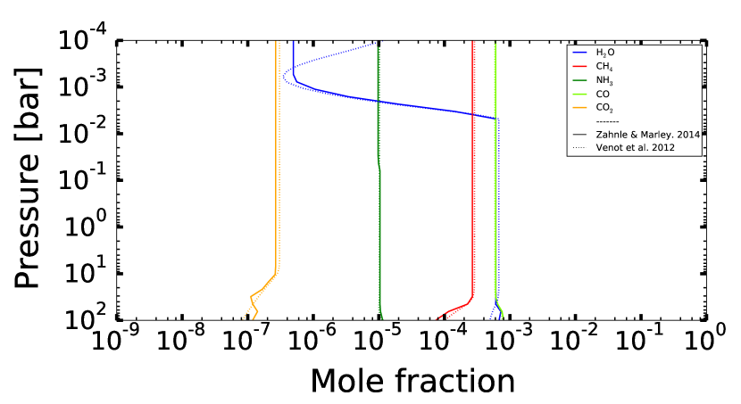
Figure 14: Abundance profiles of the defined molecules for the case GJ 504 b and K${}_{zz}=10^{11}$cm²s^-1 . Solid lines correspond to the simplified approach of Exo-REM while dotted lines correspond to the chemical kinetic model of V12.

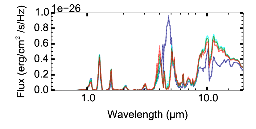
Figure 15: Emission spectra of GJ 504 b considering an atmosphere at chemical equilibrium (dark blue) and at disequilibrium ( K_zz = 10⁷, 10⁹ and 10¹¹cm²s^-1, respectively cyan, green and red). Spectra have been calculated using the chemical composition determined by the kinetic model of V12 (dotted lines) and Exo-REM (solid lines).

Figure 16: Abundance profiles for the case at 1000 K and K${}_{zz}=10^{7}cm^{2}s^{-1}$ . Solid lines correspond to the simplified approach of Exo-REM while dotted lines correspond to the chemical kinetic model of V12.

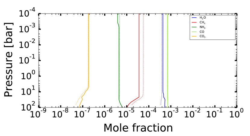
Figure 17: Abundance profiles of the defined molecules for the case VHS 1256–1257 b and K${}_{zz}=10^{11}$cm²s^-1 . Solid lines correspond to the simplified approach of Exo-REM while dotted lines correspond to the chemical kinetic model of V12.

We begin this comparison with the thermochemical equilibrium composition. In all simulated cases at equilibrium, the abundances profiles obtained with the two codes are very similar. However, we observe some differences for H₂O, CO, CH₄ (about a factor of 2 for CO and CH₄) in the deep atmosphere due to the silicate condensation taken into account in Exo-REM but not in the V12 model. To overcome this difference, we decided to apply a modification of the initial elemental abundances used in V12, in all the cases of this section, corresponding to a sequestration of $\sim$20% of the amount of oxygen in silicates (see in Appendix A, Figs. 5 a, 29 a, 30 are after the correction).

For the non-equilibrium cases, the abundance profiles show us that for the two self-luminous targets we have a good agreement. But this is not the case for the atmospheric model corresponding to T_eff=1000 K (Fig. 16, and, in Appendix A, Fig. 28 b-d). In fact we observe a strong difference in CO and CO₂ treatment (we find 1000$\times$ more CO with V12), coming from the fact that ZM14, designed for self-luminous planets, do not address the kinetic inhibition against oxidizing CH₄ (we find 18$\%$ less CH₄ with V12) to CO contrary to V12.

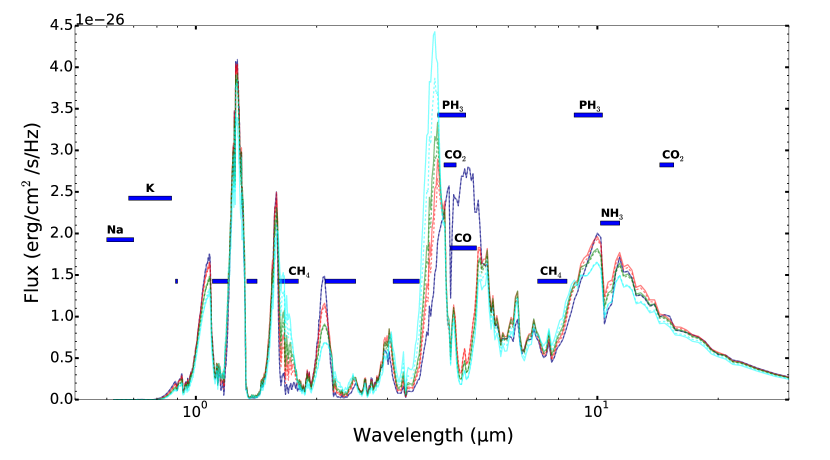
Figure 18: Emission spectra of VHS 1256–1257 b at chemical equilibrium (dark blue), or in non-equilibrium chemistry (K_zz = 10⁷, 10⁹ and 10¹¹ cm² s^-1, respectively cyan, green and red) with our two chemical models. Location of molecular features, other than H₂O, are indicated. Solid lines correspond to the simplified approach of Exo-REM while dotted lines correspond to the chemical kinetic model of V12.

Other specific and limited differences arise from different physical assumptions in the two models. For GJ 504 b, up to an altitude corresponding to 8 mbar there is a clear effect of water cold trap (see description of Exo-REM in Sect. 2) with Exo-REM, not seen in V12 where it is not used (Fig. 14 and, in Appendix A, Fig. 29). In the other side at the top all atmosphere at $K_{\mathrm{zz}}$=$10^{7}$ cm² s^-1 the difference comes from molecular diffusion, not implemented in Exo-REM (this difference appears at pressures lower than shown in the figures). Condensation of NH₃ is also a difference, Exo-REM takes into account the possibility of NH₄Cl and NH₄SH formation, explaining the difference at 8 mbar for VHS 1256–1257 b and 40 mbar for GJ 504 b (V12 does not consider these species, Figs. 14, 17 and, in Appendix A, Figs. 29 b-d, 30 b-d).

While not obvious for GJ 504 b (Fig. 14), for VHS 1256–1257 b (Fig. 17) we see a difference coming from the fact that the V12 approach exactly computes the quenching process (giving a realistic transition across the region of chemical quenching) when compared to Exo-REM where the quenching level is imposed at one precise location. We observe more water (10 $\%$) and less methane (50 $\%$) up to 1 bar in Exo-REM.

To conclude, for directly imaged planets the two chemical approaches give similar results, but this comparison confirms that Exo-REM, which uses the approach of ZM14, is not adapted to study the chemical composition of irradiated planets.

Effect on emission spectra

In this part, we detail the effect of non-equilibrium chemistry, on emission and transmission spectra.

Figures 15 and 18 present spectra obtained with the abundance profiles showed in Figs. 14, and 17. We can observe that the two chemical approaches (V12 and Exo-REM) yield very similar spectra. It is difficult to differentiate them and the differences are within the error bars expected for VHS 1256–1257 b introduced in Fig. 4. High altitude departures observed in the abundance profiles (see previous subsection) have no visible effect on the spectra because there is not enough material to absorb efficiently at pressures lower than 1 mbar.

6.4 Intrinsic effect of non-equilibrium chemistry

We use Exo-REM in the full benchmark condition except for the non-equilibrium chemistry to compute GJ 504 b emission spectra, and the full petitCODE (no constrained to benchmark conditions), combined with V12 non-equilibrium chemistry (and also at equilibrium) for the ”Guillot” 1000 K case in emission and transmission.

Important differences are observed between equilibrium and non-equilibrium chemistry at two locations of the spectrum: between 4 and 5 $\mu$m, and between 8 and 20 $\mu$m. The first location is dominated by absorption of PH₃, CO and CO₂, in out-of-equilibrium chemistry conditions. In the mid-infrared it seems easier to discriminate between out-of-equilibrium cases regarding $K_{\mathrm{zz}}$. CH₄ and NH₃ have the biggest impact at this location and the depth of the line of the latter near 10 $\mu$m offer a possible way of constraining $K_{\mathrm{zz}}$ (Figs. 15, 18). PH₃ impacts also the wavelength range just beyond 10 $\mu$m, and at 15 $\mu$m the signature of CO₂ appears with non-equilibrium chemistry (Fig. 15).

The coronagraphic mode of JWST’s MIRI instrument has been designed to be sensitive to the depth of the NH₃ feature, especially between the bottom (10.65 $\mu$m) and the edge of the band at (11.4 $\mu$m)(Figs. 15, 18).The depth of this feature seems to be a good way to investigate non- equilibrium chemistry.

Keeping in mind the fact that temperature profiles of GJ 504 b (Fig. 15) and VHS 1256-1257 b (Fig. 18), for each $K_{\mathrm{zz}}$, are computed self-consistently, we see some differences in the spectral energy distribution. This occurs because the model computes the spectrum by keeping the same integrated spectrum (i.e. $T_{\mathrm{eff}}$). The difference between non-equilibrium and equilibrium chemistry is more important for GJ 504 b; around 10 $\mu$m we observe a difference of 50 $\%$ between equilibrium and non-equilibrium cases, but the normalised spectra of the non-equilibrium cases don’t show a lot of variation (Fig. 15). It seems to be easier to determine the $K_{\mathrm{zz}}$ with the VHS 1256–1257 b spectrum (spectra around 10 $\mu$m exhibit more variation in flux and the depth of NH₃ line is more dependent on the considered $K_{\mathrm{zz}}$, Fig. 18).

In a low $T_{\mathrm{eff}}$ case (Fig. 15), non-equilibrium chemistry has an important global effect weakly dependent on the eddy coefficient (the non–equilibrium effect is something like saturated). At higher $T_{\mathrm{eff}}$ (Fig. 18) non-equilibrium chemistry has less effect but deep and hot molecules are effectively transported, proportionally to the $K_{\mathrm{zz}}$, to the top of the atmosphere. For GJ 504 b (Fig. 15) around 10 $\mu$m the three spectra at non-equilibrium just seem to be shifted without any strong shape modification. In VHS 1256–1257 b (Fig. 18) the shape of the NH₃ features varies significantly with the $K_{\mathrm{zz}}$, with a significant effect of PH₃ on the low-wavelength wing.

PH₃ is the only molecule included in Exo-REM and not in V12 with a profile impacted by non-equilibrium chemistry (it is not the case for the alkalis). In this paragraph we study the effect of PH₃ on the spectra.

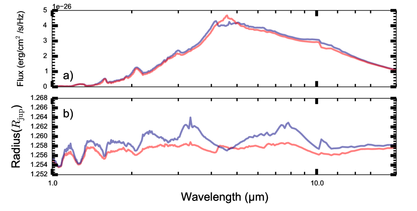
Figure 19: Emission (up) and transmission (bottom) spectra of the test exoplanet with a $T_{\mathrm{eff}}$=1000 K, computed by petitCODE using equilibrium chemistry (blue) or non equilibrium with K_zz=10¹¹ cm²s^-1 (red) using V12.

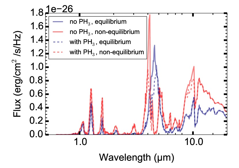
Figure 20: Spectra of GJ 504 b, computed by Exo-REM with and without PH₃, assuming thermochemical equilibrium or in non-equilibrium conditions ($K_{\mathrm{zz}}$=10¹¹cm²s^-1) with the same PT profile (case with PH₃ at equilibrium)

We compute first the full model of GJ 504 b with Exo-REM, at equilibrium, with PH₃. Then we use the obtained PT profile in this first case in Exo-REM to generate spectra at equilibrium or with K_zz=10¹¹cm²/s, with or without PH₃. Figure 20 shows all the corresponding spectra. We see the effect of phosphine around 4.5 and 9 $\mu$m. At thermochemical equilibrium the right wing of the PH₃ feature is visible at 4.5 $\mu$m but the signature of PH₃ at 9 $\mu$m is completely hidden by the ammonia absorption. In the case of non–equilibrium chemistry both PH₃ features are visible, especially the left wing around 4.5 $\mu$m, but the red wing is hidden by CO and CO₂.

7 Influence of the differing model assumptions on the analysis of JWST observations

In this section we quantify differences coming from the previously identified model differences and compare them with the expected direct imaging uncertainties of JWST observations. For this analysis we use the signal-to-noise ratio (S/N) that we previously estimated for the NIRSpec and MIRI instrument modes, described for Fig. 4 in Sec. 4.1 for VHS 1256–1257 b.

We compute the $\chi^{2}$ in the wavelength range where we observe an effect between the average spectrum (between all the approaches) and the other spectra taken separately. We perform, in parallel, a Kolmogorov–Smirnov test (KStest) as done in Mollière et al. (2017). If the $\chi^{2}$ or the $p_{\mathrm{KStest}}$ is around 1, then the differences between the approaches correspond to the uncertainties of the JWST. If, on the other hand, $\chi^{2}>>1$ or $p_{\mathrm{KStest}}<<1$, then the differences between the approaches are larger than the JWST uncertainties.

First, for the different alkali line profiles, we use the spectra plotted in Figs. 6 and 9, restrained to the wavelength range between 0.6 and 0.9 $\mu$m (i.e. in the part of the NIRSpec range that is mostly impacted by alkalies).

We find that, in the case of directly imaged exoplanet, the average $\chi^{2}$, as defined as above, is always larger than 20 and ($p_{\mathrm{KStest}}$ is lower than $10^{-30}$).

Therefore, the precision expected with JWST allows us to hope to be able to learn more about the profile of the alkalies even if this wavelength range is also impacted by the clouds (we don’t study this effect in the paper).

We focus then on the effect of the selection of a given molecular far wing lineshape, using the spectra plotted in Fig. 12. We combine here wavelength ranges from NIRSpec and MIRI: 0.6-13.9 $\mu$m (the same as for VHS 1256–1257 b previously used in this paper).

For a directly imaged planet, we find that using or not a far wing cut-off yields a significant difference (average $\chi^{2}>20$ and $p_{\mathrm{KStest}}<10^{-9}$).

The effect is more important in spectral windows outside the main molecular features, acting like a continuum, and may induce uncertainties in the retrievals of some atmospheric parameters, such as clouds parameters, larger than those due to the uncertainties on the data themselves.

For directly imaged planets, differences between equilibrium and out of equilibrium compositions (K_zz=10¹¹cm²/s) are largely higher than the observational uncertainties (the average $\chi^{2}$ is over 15 and $p_{\mathrm{KStest}}<10^{-4}$). It should be possible to determine what is the chemical regime of the observed atmosphere.

Finally we focus on PH₃, in two wavelength ranges, 4-6 (NIRSpec) and 9-10 (MIRI) $\mu$m using Fig. 20. This molecule has a strong effect on the observable spectra and it should be easy to discriminate whether the atmosphere contains PH₃ or not (with a minimal average $\chi^{2}$ of 40 and $p_{\mathrm{KStest}}<10^{-10}$).

8 Conclusions and perspectives

The forthcoming JWST will open a new era to characterize exoplanet atmospheres. The observed spectra with the high signal-to-noise ($>$ 100 for exoplanets detected in direct imaging such as VHS 1256-1257 b) expected with the JWST instruments will require precise and well tested models to interpret the results. We need to be able to understand differences between models. To do that we define in this paper a benchmark protocol.

We compared and updated three radiative-convective equilibrium models (ATMO, Exo-REM and petitCODE) and compared two chemical models (V12 and Exo-REM). We showed that the analysis of JWST observations will be sensitive to differences in the modelling of some key parameters introduced in the various models. This fact should be kept in mind when drawing conclusions.

Many iterations were needed to achieve similar results in our benchmark conditions. We have spotted the importance of PH₃ in atmospheres, and also the crucial need of complete molecular linelists. Exomol is often considered as the most up-to-date database currently available, and is indeed better adapted to hot atmospheres than Hitran (built for Earth-like temperatures). However, the current version of Exomol is not the ultimate linelist database. Improvements are still going on, for example Rey et al. (2017) for CH₄. During the definition of the benchmark protocol, we spotted that chemistry model can also imply important differences, if one takes into account ionic species at hot temperature, isotopes, etc.

The first major difference spotted early in the process was the different treatment applied for the far wing lineshape of alkali lines. The definition of the alkali treatment is crucial. Using one approach or the other can shift the temperature by more than 100 K and change the flux in spectral region where we also expect clouds effects (reddening of the spectrum observed for example in brown dwarf observations Tsuji et al., 1996). However, comparison to observations does not allow us to select the best approach.

We investigated also a second effect. We found that applying a sub-Lorentzian lineshape in the far wings of molecular species can change the resulting spectra both in transmission and emission by up to $\sim 20$ %, but usually less. This is comparable to what has been found by Grimm & Heng (2015). In the self-consistent temperature structures obtained for irradiated planets, an increased opacity (due to neglecting the cut-off) leads to an inverse green house effect in the atmosphere, because less stellar radiation is absorbed in the deep atmosphere if full Voigt profiles are used. Uncertainties in the far wing lineshape is also a limitation in analysing thermal emission spectra from Solar System planetary atmospheres. This is the case for relatively transparent spectral windows, such as the methane windows in Titan between 1.3 and 5 $\mu$m (e.g. Hirtzig et al., 2013) or near-infrared windows observed on Venus’ night side between 1 and 2.3 $\mu$m (e.g. Fedorova et al., 2015). Sub-lorentzian lineshapes beyond a few wavenumbers from line core are clearly needed to reproduce the observed spectra but, precise constraints on the profiles cannot be retrieved independently of other atmosphere or surface parameters. For giant exoplanets, while sub-Lorentzian far wing profiles are also likely to occur, no prescription can be made today in the lack of laboratory measurements of H₂-broadened line far wings at high temperatures.

To compare models carefully we need to use the same alkali treatment and far wing lineshape for other absorbers.

We have also compared various chemical approaches. While we see clear differences between non-equilibrium and equilibrium abundances, we did not spot significant differences in the spectra based on the different implementations used for the two processes. The major differences occur at high altitudes: cold-trap and molecular scattering, without strong impact on the spectrum..

Among all the models parameters discussed and analysed in the paper, those having a major impact on the observable are:

• Alkali wing lineshape

• PH₃ opacity

• sub-Lorentzian lineshape

• non-equilibrium chemistry

We showed that these four modelling parameters will have an impact on spectra with differences larger than the JWST uncertainties, especially for directly imaged exoplanets. However, in the case of alkali lineshape or molecular line far wing, the differences in the modelled spectra could be translate as an artificial off-set, without an easy way to identify it.

To improve the reliability of atmospheric models, particular efforts need to be undertaken to enhance experimental and theoretical work at high pressure and high temperature conditions in terms of :

• wing lineshape, especially for alkalies

• linelist completeness

This work is urgently needed if we want to be able to interpret correctly the observations of the JWST.

We also identified some other effects coming from:

• adding isotopes

• adding ions

• using up-to-date linelists

• definition of the reference radius for transmission spectrum

• computation of the mean molecular weight

And finally the differences, spotted in the abundances profiles, without any significant spectral effect found in the analysis are:

• cold-trap

• molecular diffusion

Spectra and profiles generated for the benchmark (i.e. the data behind the Figs. 21-27 of the Appendix A) are available as supplementary material. We encourage the community to compare them to their models in these benchmark conditions and iterate with us to continue to improve our respective models and identify the existing differences.

Appendix A Complete set of figures

Following figures (Figs. 21-30) show all the radiative-convective equilibrium models in the benchmark condition (see Sects. 3 and 4).

Figure 21: Emission and transmission spectra for the case T_eff = 500 K ( respectively a) and b) ) and the cases T_eff = 1000 K ( respectively c) and d) ) with variation of metallicity ( solid = solar, small dash = 3 $\times$ solar, large dash = 30 $\times$ solar ). Exo-REM is in blue, petitCODE in green, ATMO in red.

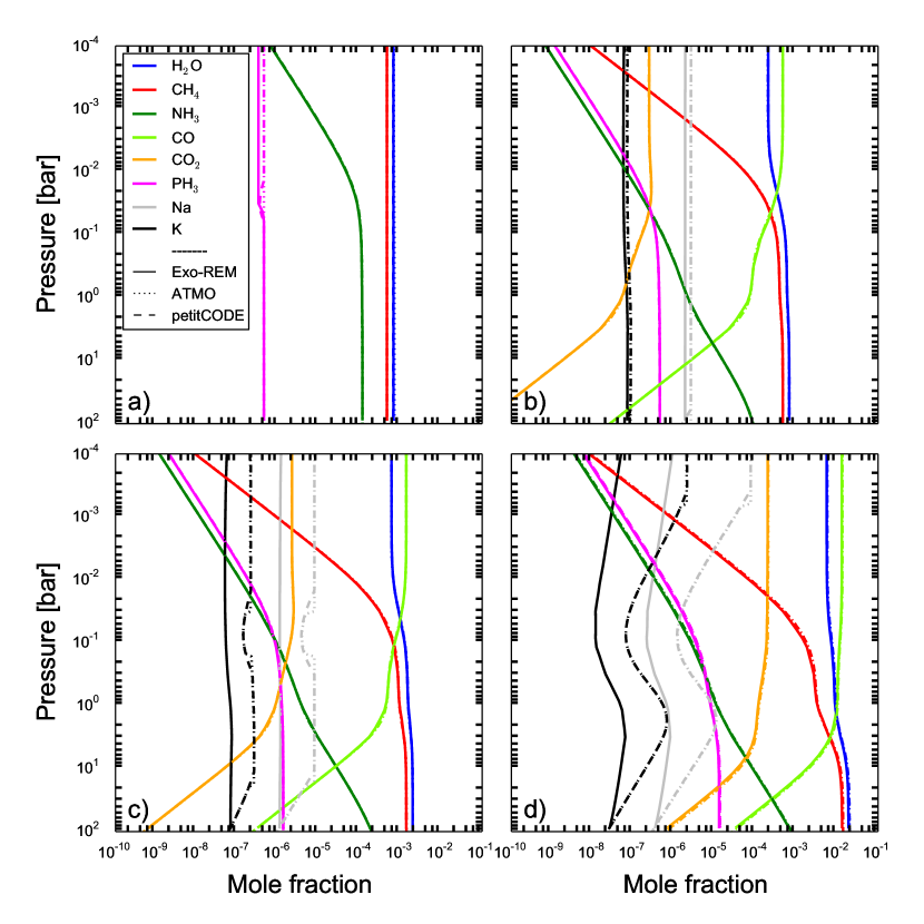
Figure 22: Abundance profiles for the case Teff = 500 K ( a) ) and the cases Teff = 1000 K with variation of metallicity ( b)solar, c) 3 $\times$ solar, d) 30 $\times$ solar).

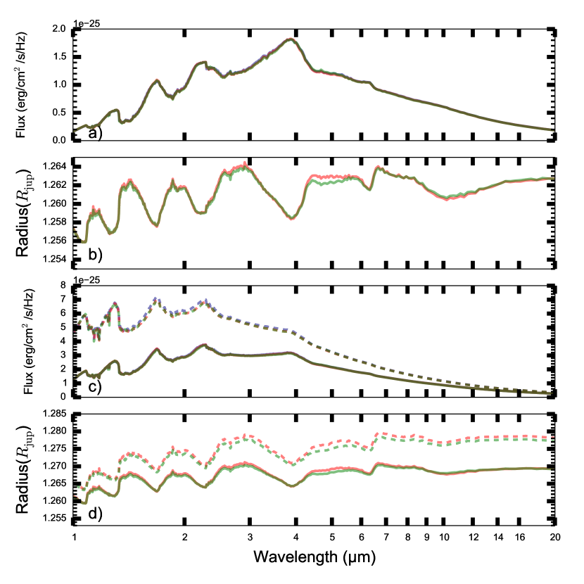
Figure 23: Emission and transmission spectra for the case T_eff = 1500 K ( respectively a) and b) ) and the cases T_eff = 2000 K (plain) and 2500 K (dash) ( respectively c) and d) ). Exo-REM is in blue, petitCODE in green, ATMO in red.

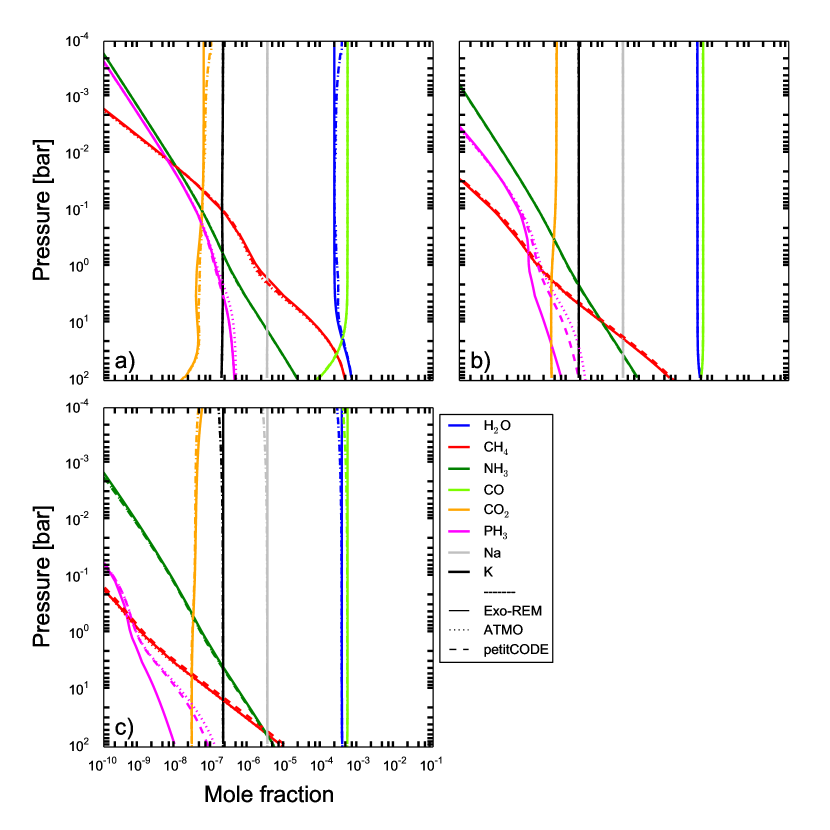
Figure 24: Abundance profiles for the cases T_eff = 1500 K ( a) ), 2000 K ( b) ) and 2500 K ( c) ).

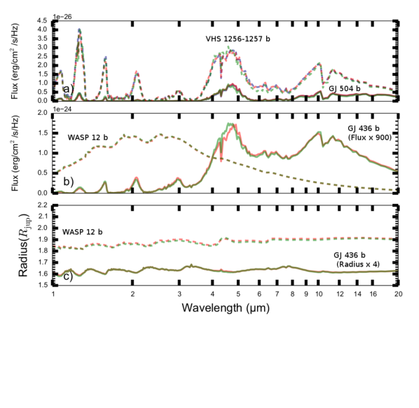
Figure 25: Emission spectra of the two directly imaged planets ( a) ). Emission ( b) ) and transmission ( c) ) spectra of the two transiting planets. For GJ 436 b the flux is multiplied by 900, and the radius by 4 to put the two cases in the same plot.

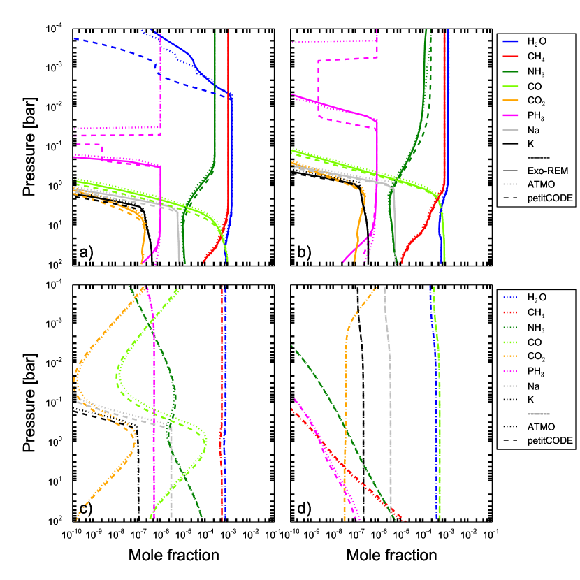
Figure 26: Abundance profiles of the potential targets: a) GJ 504 b, b) VHS 1256–1257 b, c) GJ 436 b and d) WASP 12 b.

Figure 27: Temperature profiles computed by our three models (Exo-REM is in blue, petitCODE in green, ATMO in red) of the potential targets.

They complement figures shown in Sect. 6

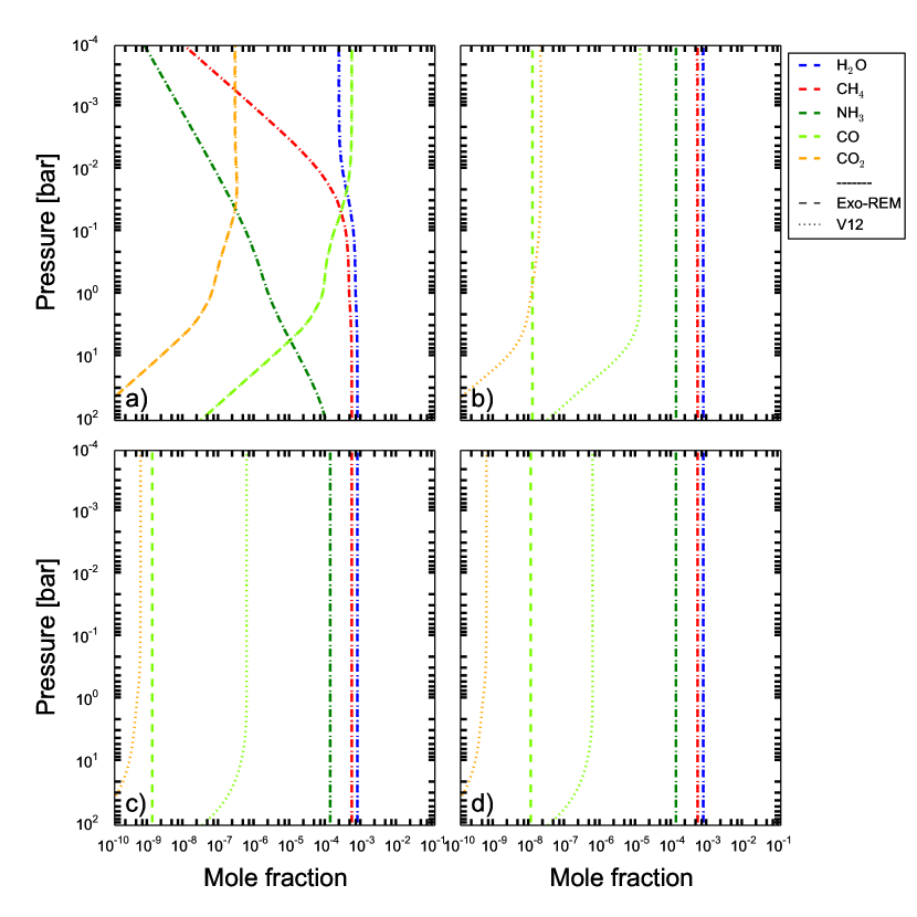
Figure 28: Abundance profiles for T_eff = 1000 K at equilibrium chemistry ( a) ) and for K_zz = 10⁷ ( b) ), 10⁹ ( c) ) and 10¹¹ ( d) ) cm² s^-1

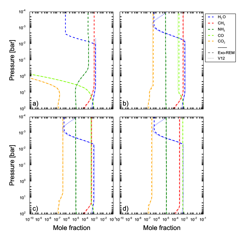
Figure 29: Abundance profiles for GJ 504 b at equilibrium chemistry ( a) ) and for K_zz = 10⁷ ( b) ), 10⁹ ( c) ) and 10¹¹ ( d) ) cm² s^-1

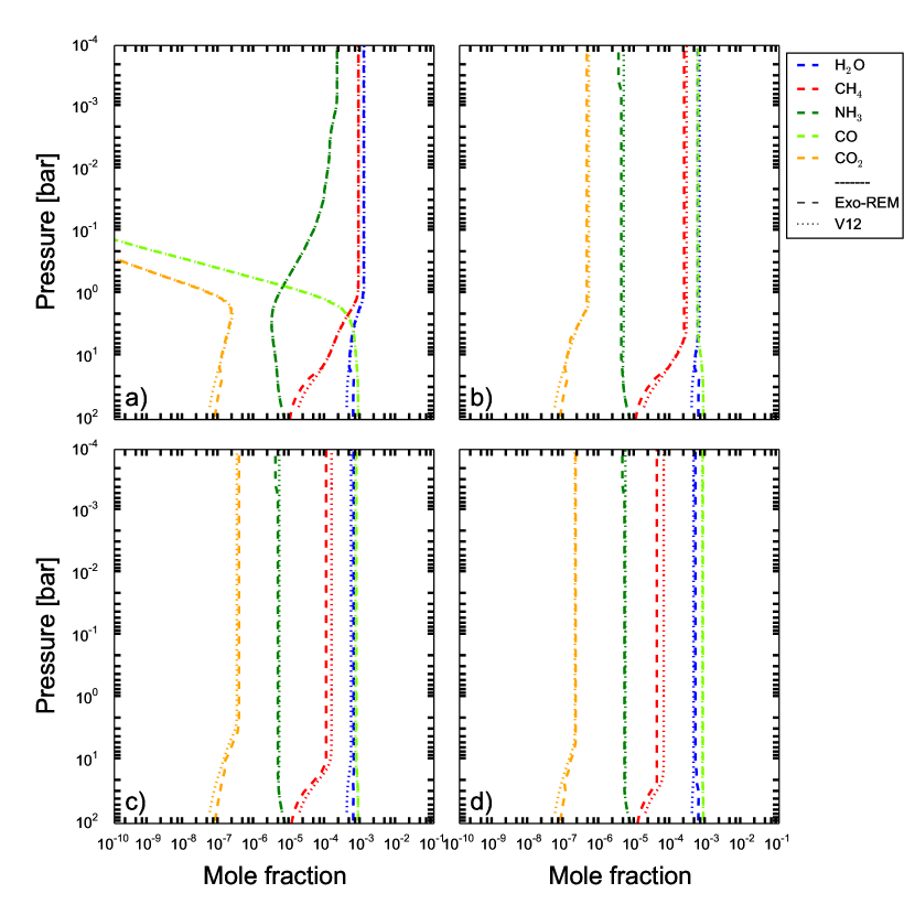
Figure 30: Abundance profiles for VHS 1256–1257 b at equilibrium chemistry ( a) ) and for K_zz = 10⁷ ( b) ), 10⁹ ( c) ) and 10¹¹ ( d) ) cm² s^-1

Appendix B Updates of Exo-REM

Exo-REM has been updated on several aspects since the version described in Baudino et al. (2015):

• Correlated k-coefficients of different molecules are now combined assuming no correlation between species in any spectral interval. This is done using the method named ”reblocking of the joint k-distribution” by Lacis & Oinas (1991) and more extensively described in Mollière et al. (2015) (”R1000” method in their Appendix B.2.1)

• CO₂ and PH₃ have been added to the list of molecular absorbers, using linelists from Rothman et al. (2013) and Sousa-Silva et al. (2015) respectively. For CO₂ pressure-broadened halfwidths ($\gamma$), we used the air-broadened values multiplied by 1.34 (Burch et al., 1969) to obtain the broadening by H₂ and He. For PH₃, we used: for $J\leq 20,\gamma=0.1009-0.00137\times J$ if $J\neq K$ and 0.9 time this result if J=K with a temperature exponent $n=0.643-0.00912\times J$; for $J>20$, we fixed $\gamma=0.073$ and $n=0.46$. Relevant references are Levy et al. (1993), Salem et al. (2004) and Levy et al. (1994).

• Collision-Induced Absorption (CIA) of H₂-H₂ and H₂-He is now modeled following HITRAN (Richard et al., 2012), complemented for H₂-H₂ beyond 10000 cm^-1 by Borysow et al. (2001) and Borysow (2002) with a small rescaling to ensure continuity at 10000 cm^-1.

References

- Allard et al. (2007) Allard, N. F., Kielkopf, J. F., & Allard, F. 2007, EPJD, 44, 507
- Allard et al. (2012) Allard, N. F., Kielkopf, J. F., Spiegelman, F., Tinetti, G., & Beaulieu, J. P. 2012, A&A, 543, A159
- Allard et al. (1999) Allard, N. F., Royer, A., Kielkopf, J. F., & Feautrier, N. 1999, PhRvA, 60, 1021
- Allard et al. (2016) Allard, N. F., Spiegelman, F., & Kielkopf, J. F. 2016, A&A, 589, A21
- Amundsen et al. (2016) Amundsen, D., Tremblin, P., Manners, J., Baraffe, I., & Mayne, N. 2016, A&A, doi:10.1051/0004-6361/201629322
- Amundsen et al. (2014) Amundsen, D. S., Baraffe, I., Tremblin, P., et al. 2014, A&A, 564, A59
- Asplund et al. (2009) Asplund, M., Grevesse, N., Sauval, A. J., & Scott, P. 2009, ARA&A, 47, 481
- Barber et al. (2006) Barber, R. J., Tennyson, J., Harris, G. J., & Tolchenov, R. N. 2006, MNRAS, 368, 1087
- Barman et al. (2015) Barman, T. S., Konopacky, Q. M., Macintosh, B., & Marois, C. 2015, ApJ, 804, 61
- Barman et al. (2011) Barman, T. S., Macintosh, B., Konopacky, Q. M., & Marois, C. 2011, ApJ, 733, 65
- Baudino et al. (2015) Baudino, J.-L., Bézard, B., Boccaletti, A., et al. 2015, A&A, 582, A83
- Borysow (2002) Borysow, A. 2002, A&A, 390, 779
- Borysow et al. (2001) Borysow, A., Jørgensen, U. G., & Fu, Y. 2001, JQSRT, 68, 235
- Burch et al. (1969) Burch, D. E., Gryvnak, D. A., Patty, R. R., & Bartky, C. E. 1969, JOSA (1917-1983), 59, 267
- Burch et al. (1969) Burch, D. E., Gryvnak, D. A., Patty, R. R., & Bartky, C. E. 1969, JOSA, 59, 267