Interactive Visual Data Exploration with Subjective Feedback: An Information-Theoretic Approach

Abstract

Visual exploration of high-dimensional real-valued datasets is a fundamental task in exploratory data analysis (EDA). Existing methods use predefined criteria to choose the representation of data. There is a lack of methods that (i) elicit from the user what she has learned from the data and (ii) show patterns that she does not know yet. We construct a theoretical model where identified patterns can be input as knowledge to the system. The knowledge syntax here is intuitive, such as “this set of points forms a cluster”, and requires no knowledge of maths. This background knowledge is used to find a Maximum Entropy distribution of the data, after which the system provides the user data projections in which the data and the Maximum Entropy distribution differ the most, hence showing the user aspects of the data that are maximally informative given the user’s current knowledge. We provide an open source EDA system with tailored interactive visualizations to demonstrate these concepts. We study the performance of the system and present use cases on both synthetic and real data. We find that the model and the prototype system allow the user to learn information efficiently from various data sources and the system works sufficiently fast in practice. We conclude that the information theoretic approach to exploratory data analysis where patterns observed by a user are formalized as constraints provides a principled, intuitive, and efficient basis for constructing an EDA system.

I Introduction

Figure 1: Overview of the interaction process.

(a)	(b)	(c)

Figure 2: Synthetic data with 3 dimensions. (a) Projection of the data to the first two principal components together with a sample of background distribution; (b) After the user’s knowledge is taken into account, the updated background distribution matches the data in this projection; (c) The user is then shown the next most informative projection.

Ever since Tukey’s pioneering work on exploratory data analysis (EDA) [1], effective exploration of data has remained an art as much as a science. Indeed, while human analysts are remarkably skilled in spotting patterns and relations in adequately visualized data, coming up with insightful visualizations is hard task to formalize, let alone to automate.

As a result, EDA systems require significant expertise to use effectively. However, with the increasing availability and importance of data, data analysts with sufficient expertise are becoming a scarce resource. Thus, further research into automating the search for insightful data visualizations is becoming increasingly critical.

Modern computational methods for dimensionality reduction, such as Projection Pursuit and manifold learning, allow one to spot complex relations from the data automatically and to present them visually. Their drawback is however that the criteria by which the views are found are defined by static objective functions. The resulting visualizations may or may not be informative for the user and task at hand. Often such visualizations show the most prominent features of the data, while the user might be interested in other subtler structures. It would therefore be of a great help if the user could efficiently tell the system what she already knows and the system could utilize this when deciding what to show the user next. Achieving this is the main objective of this paper.

We present a novel interaction system based on solid theoretical principles. The main idea of the system is shown in Fig. 1. The computer maintains a distribution, called the background distribution (1a), modelling the belief state of the user. The system shows the user projections in which the data and the background distribution differ the most (1b,c). The user marks in the projection the patterns she has observed (1d,e) and the computer then uses these to update the background distribution (1f). The process is iterated until the user is satisfied, i.e., typically when there are no notable differences between the data and the background distribution.

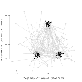
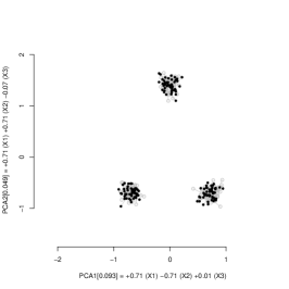
Example. Specifically, the data considered in this work is a set of $d$-dimensional ($d$-D) data points. To illustrate the envisioned data exploration process, we synthesized a 3-D dataset with 150 points such that there are two clusters of 50 points and two of 25 points. The smaller clusters are partially overlapping in the third dimension. Looking at the first two principal components, one can only observe three clusters with 50 points each (similarly to the black points in Fig. 2a).

In our interactive approach, the data analyst will learn not only that there are actually four clusters, but also that two of the four clusters correspond to a single cluster in the first view of the data. The visualizations considered are scatter plots of the data points after projection onto a 2-D subspace, as in Projection Pursuit [2, 3]. The projection chosen for visualization is the one that (for a certain statistic) is maximally different with respect to the background distribution that represents the user’s current understanding of the data.

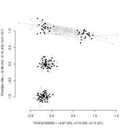
In addition to showing the data in the scatterplot, we display a sample from the background distribution as gray points (and lines that connect the respective points, to give an indication of the displacement in the background distribution, per data point); see Fig. 2 for an example and Sec. III for details. The data analyst’s interaction consists of informing the system about sets of data points they perceive to form clusters within this scatter plot. The system then takes the information about the user’s knowledge of the data into account and updates the background distribution accordingly (Fig. 2b).

When we have ascertained ourselves that the background distribution matches the data in the projection as we think it should, the system can be instructed to find another 2-D subspace to project the data onto. The new projection displayed is the one that is maximally insightful considering the updated background distribution. The next projection is shown in Fig. 2c and reveals that one of the three clusters from the previous view can in fact be split into two. The user can now add further knowledge to the background distribution by selecting the two uppermost clusters and the process can be repeated. For our 3-D dataset, after the background distribution is updated upon addition of the new knowledge, the data and the background distribution match, and in this case, further projections will not reveal any additional structure.

Figure 3: A pairplot of the synthetic data $\hat{\bf X}_{5}$. Colors correspond to the cluster identities $A,B,C$, and $D$ (the grouping that exists in the first three dimensions). Plot based on a sample of 250 points from the data.

I-A Contributions and outline of the paper

The contributions of this paper are:

• We review how to formalize and efficiently find a background distribution accounting for a user’s knowledge, in terms of a constrained Maximum Entropy distribution.

• A principled way to obtain projections showing the maximal difference between the data and the background distribution for the PCA and ICA objectives, by whitening the data with respect to the background distribution.

• An interaction model by which the user can input what she has learned from the data, in terms of constraints.

• An experimental evaluation of the computational performance of the method and use cases on real data.

• A free open source application demonstrating the method.

The paper is structured as follows: we describe the method and the algorithms in Sec. II, present the proof-of-concept open source implementation sideR in Sec. III, report the results of the experiments in Sec. IV, discuss the related work in Sec. V, and finally conclude in Sec. VI.

II Methods

II-A Maximum Entropy background distribution

Preliminaries. The dataset consists of $n$ $d$-dimensional real vectors $\hat{\bf x}_{i}\in{\mathbb{R}}^{d}$, where $i\in[n]=\{1,\ldots,n\}$. The whole dataset is represented by a real-valued matrix $\hat{\bf X}=\left(\hat{\bf x}_{1}\hat{\bf x}_{2}\ldots\hat{\bf x}_{n}\right)^{T}\in{\mathbb{R}}^{n\times d}$. We use hatted variables (e.g., $\hat{\bf X}$) to denote the observed data and non-hatted variables to denote the respective random variables (e.g., ${\bf X}$).

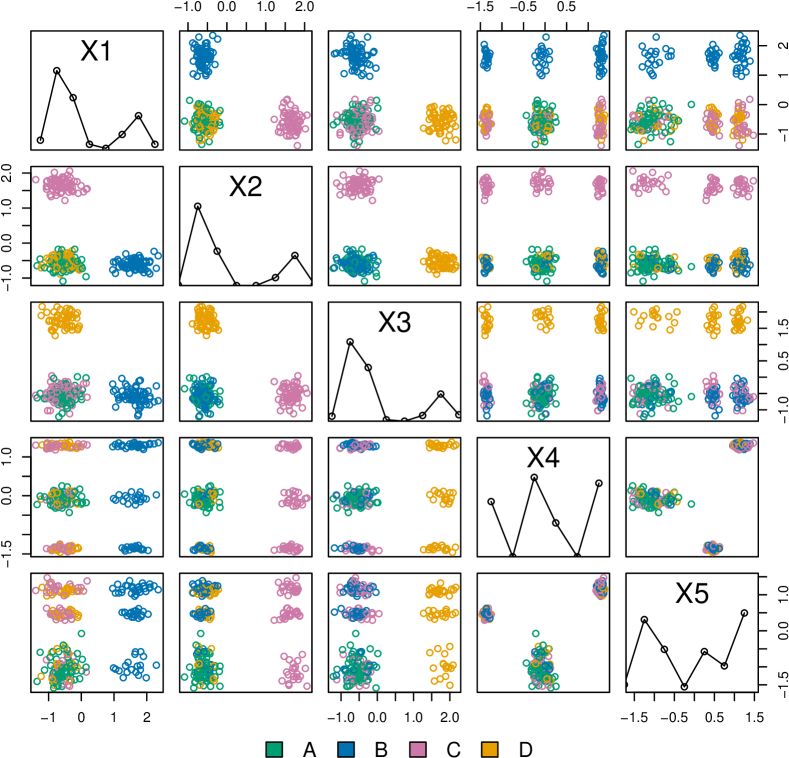
Running example (Fig. 3). To illustrate the central concepts of the approach, we generated a synthetic dataset $\hat{\bf X}_{5}$ of 1000 data vectors in five dimensions. The dataset is designed so that along dimensions 1–3 it can be clustered into four clusters (labeled $A,B,C,D$) and along dimensions 4–5 into three clusters (labeled $E,F,G$). The clusters in dimensions 1–3 are located such that in any 2-D projection along these dimensions cluster $A$ overlaps with one of the clusters $B,C$, or $D$. The cluster structure in dimensions 4–5 is loosely related to the cluster structure in dimensions 1–3: with 75% probability a data vector belonging to clusters $B,C$, or $D$ belongs to one of clusters $E$ and $F$. The remaining points belong to cluster $G$. The pairplot in Fig. 3 shows the structure of the data (colors correspond to the cluster identities A, B, C, D).

Constraints. To implement the envisioned interaction scheme, we wish to define constraints on the data and to find a Maximum Entropy distribution such that the constraints set by the user are satisfied. Intuitively, the more constraints we have, the closer the distribution should be to the true data.

We must define some initial background distribution. Reasonable and convenient is to assume that the initial background distribution equals a spherical Gaussian distribution with zero mean and unit variance, given by

$$q({\bf X})\propto\exp{\left(-\sum\nolimits_{i=1}^{n}{{\bf x}_{i}^{T}{\bf x}_{i}}/2\right)}.$$ (1)

Example 1.

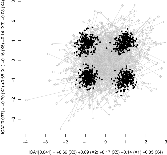
As illustrated in Fig. 1, the interaction process is such that the user is shown 2-D projections (1c) where the data and the background distribution differ the most. Initially, when there is no knowledge about the belief state of the user, the background distribution (1a) is assumed to be a spherical Gaussian distribution with zero mean and unit variance. The initial view shown to the user is a projection of the data onto the first two PCA or ICA components. Fig. 4a shows the projection of $\hat{\bf X}_{5}$ onto the first two ICA components. One can observe the cluster structure in the first three dimensions. The gray points represent a sample from the background distribution. When shown together with the data, it becomes evident that the data and the background distribution differ.

Subsequently, we can define constraints on subsets of points in ${\mathbb{R}}^{n\times d}$ for a given projection by introducing linear and quadratic constraint functions [4]. A constraint is parametrized by the subset of rows $I\subseteq[n]$ that are involved and a projection vector $\mathbf{w}\in\mathbb{R}^{d}$. The linear constraint function is defined by

$$f_{\textrm{lin}}(\mathbf{X},I,\mathbf{w})=\sum\nolimits_{i\in I}{\mathbf{w}^{T}\mathbf{x}_{i}},$$ (2)

and the quadratic constraint function by

$$f_{\textrm{quad}}(\mathbf{X},I,\mathbf{w})=\sum\nolimits_{i\in I}{\left(\mathbf{w}^{T}\left(\mathbf{x}_{i}-\mathbf{\hat{m}}_{I}\right)\right)^{2}},$$ (3)

where we have used

$$\mathbf{\hat{m}}_{I}=\sum\nolimits_{i\in I}{\mathbf{\hat{x}}_{i}}/|I|.$$ (4)

Notice that $\mathbf{\hat{m}}_{I}$ is not a random variable but a constant that depends on the observed data. If it were a random variable it would introduce cross-terms between rows and the distribution would no longer be independent for different rows. In principle, we could set $\mathbf{\hat{m}}$ to any constant value, including zero. However, for the numerical algorithm to converge quickly we use the value specified by Eq. (4).

We can use the linear and quadratic constraint functions to define several types of knowledge a user may have about the data, which we can then encode into the Maximum Entropy background distribution.

We can encode the mean and variance, i.e., the first and second moment of the marginal distribution, of each attribute:

• Margin constraint consists of a linear and a quadratic constraint for each of the columns in $[d]$, respectively, the total number of constraints being $2d$.

We can encode the mean and (co)variance statistics of a point cluster for all attributes:

• Cluster constraint is defined as follows. We make a singular value decomposition (SVD) of the points in the cluster defined by $I$. Then a linear and a quadratic constraint is defined for each of the eigenvectors. This results in $2d$ constraints per cluster.

We can encode the mean and (co)variance statistics of the full data for all attributes:

• 1-cluster constraint is a special case of a cluster constraint where the full dataset is assumed to be in one single cluster (i.e., $I=[n])$. Essentially, this means that the data is modeled by its principal components and the correlations are taken into account, unlike with the marginal constraints, again resulting to $2d$ constraints.

We can encode the mean and variance of a point cluster or the full data as shown in the current 2-D projection:

• 2-D constraint consists of a linear and a quadratic constraint for the two vectors spanning the 2-D projection in question, resulting to $4$ constraints.

The background distribution. We denote a constraint by a triplet $C=(c,I,\mathbf{w})$, where $c\in\{lin,quad\}$, and the constraint function is then given by $f_{c}(\mathbf{X},I,\mathbf{w})$. Our main problem, i.e., how to update the background distribution given a set of constraints, can be stated as follows.

Problem 1.

Given a dataset $\mathbf{\hat{X}}$ and $k$ constraints $\mathcal{C}=\{C^{1},\ldots,C^{k}\}$, find a probability density $p$ over datasets ${\bf X}\in{\mathbb{R}}^{n\times d}$ such that the entropy defined by

$$S=-E_{p({\bf X})}\left[\log{\left(p({\bf X})/q({\bf X})\right)}\right]$$ (5)

is maximized, while the following constraints are satisfied for all $t\in[k]$,

$$E_{p(\mathbf{X})}\left[f_{c^{t}}(\mathbf{X},I^{t},\mathbf{w}^{t})\right]=\hat{v}^{t},$$ (6)

where $\hat{v}^{t}=f_{c^{t}}(\mathbf{\hat{X}},I^{t},\mathbf{w}^{t})$.

We call the distribution $p$ that is a solution to the Prob. 1 the background distribution. Intuitively, the background distribution is the maximally random distribution such that the constraints are preserved in expectation. The form of the solution to Prob. 1 is given by the following lemma.

Lemma 1.

The probability density $p$ that is a solution to Prob. 1 is of the form

$$p({\bf X})\propto q({\bf X})\times\exp{\left(\sum\nolimits_{t=1}^{k}{\lambda^{t}f_{c^{t}}({\bf X},I^{t},{\bf w}^{t})}\right)},$$ (7)

where $\lambda^{t}\in{\mathbb{R}}$ are real-valued parameters.

See, e.g., Ch. 6 of [5] for a proof.

We make an observation that adding a margin constraint or 1-cluster constraint to the background distribution is equivalent to first transforming the data to zero mean and unit variance or whitening of the data, respectively.

Eq. (7) can also be written in the form

$$p({\bf X}\mid\theta)\propto\exp{\left(-\sum\nolimits_{i=1}^{n}{\left({\bf x}_{i}-{\bf m}_{i}\right)^{T}\Sigma_{i}^{-1}\left({\bf x}_{i}-{\bf m}_{i}\right)/2}\right)},$$ (8)

where the natural parameters are collectively denoted by $\theta=\left\{\theta_{i}\right\}_{i\in[n]}=\left\{\left(\Sigma^{-1}_{i}{\bf m}_{i},\Sigma_{i}^{-1}\right)\right\}_{i\in[n]}$, which can be written as sums of the terms of the form $\lambda^{t}f_{c^{t}}({\bf X},I^{t},{\bf w}^{t})$ by matching the terms linear and quadratic in ${\bf x}_{i}$ in Eqs. (7) and (8). The dual parameters are given by $\mu=\left\{\mu_{i}\right\}_{i\in[n]}=\left\{\left({\bf m}_{i},\Sigma_{i}\right)\right\}_{i\in[n]}$ and can be obtained from the natural parameters by simple matrix operations (see below).

Prob. 1 can be solved numerically as follows. Initially, we set the lambda parameters to $\lambda_{1}=\ldots=\lambda_{k}=0$, with the natural dual parameters then given by $\theta_{i}=\mu_{i}=\left({\bf 0},{\bf 1}\right)$ for all $i\in[n]$. We then update the lambda parameters iteratively as follows. Given some values for the lambda parameters and the respective natural and dual parameters, we choose a constraint $t\in[k]$ and find a value for $\lambda^{t}$ such that the constraint of Eq. (6) is satisfied for this chosen $t$. We then iterate this process for all constraints $t\in[k]$ until convergence. Due to convexity of the problem we are always guaranteed to eventually end up in a globally optimal solution.

For a given set of lambda parameters we can find the natural parameters in $\theta$ by a simple addition. The dual parameters can be obtained from the natural parameters, e.g., by using matrix inversion and multiplication operations. The expectation in Eq. (6) can be computed by using the dual parameters and identities $E_{p({\bf X}\mid\theta)}\left[{\bf x_{i}}{\bf x_{i}}^{T}\right]=\Sigma_{i}+{\bf m}_{i}{\bf m}_{i}^{T}$ and $E_{p({\bf X}\mid\theta)}\left[{\bf x}_{i}\right]={\bf m}_{i}$.

(a)	(b)
(c)	(d)

Figure 4: (a) The synthetic data $\hat{\bf X}_{5}$ projected into the first two ICA components and shown together with a sample of the background distribution (in gray). With no knowledge about the belief state of the user, the background distribution is Gaussian. (b) The same projection with the background distribution updated to take into account cluster constraints for the four visible clusters. (c) The next most informative ICA projection for $\hat{\bf X}_{5}$. (d) The ICA projection obtained after further cluster constraints for the three visibile clusters have been added and the background distribution has been updated.

Example 2.

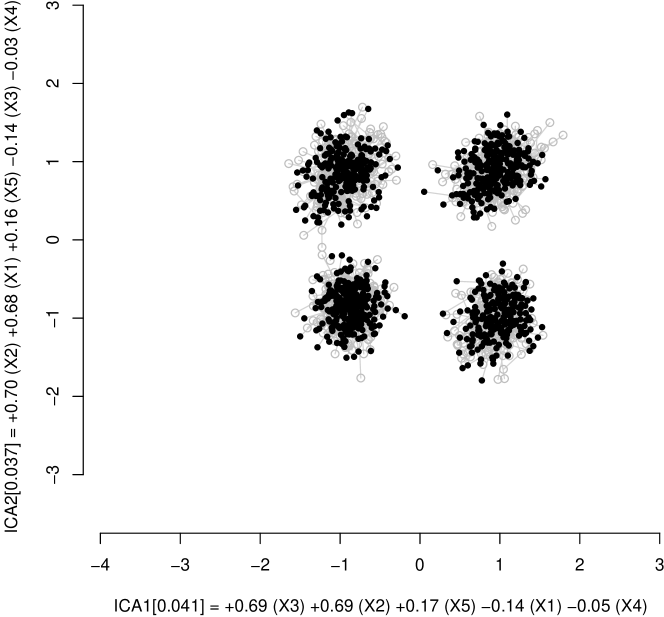
After observing the view in Fig. 4a the user can add a cluster constraint for each of the four clusters visible in the view. The background distribution is then updated to take into account the added constraints by solving Prob. 1. In Fig. 4b a sample of the updated background distribution (gray points) is shown together with the data (black points).

(a)

(b)

Figure 5: (a) Adversarial toy data and $1\sigma$ confidence ellipsoids (expanded a bit for visual clarity in zero variance directions) for the background distribution. (b) Convergence of $(\Sigma_{1})_{11}$ for two sets of constraints ${\mathcal{C}}_{A}$ (black line) and ${\mathcal{C}}_{B}$ (red line).

The straightforward implementation of the above mentioned optimization process is inefficient because we need to store parameters for $n$ rows and and because the matrix inversion is an $O(d^{3})$ operation, resulting to a time complexity of $O(nd^{3})$.

We can substantially speed up the computations by two observations. First, two rows affected by the same constraints share equal parameters. We need only to store and compute values of the parameters $\theta_{i}$ and $\mu_{i}$ for “equivalence classes” of rows, whose number depends on the number and overlap of constraints, but not on $n$. Second, if we store both the natural and dual parameters at each iteration, the constraint at an iteration corresponds to a rank-1 update to the covariance matrix $\Sigma^{-1}_{i}$. We can then use the Woodbury Matrix Identity taking $O(d^{2})$ time to compute the inverse, instead of $O(d^{3})$.

Moreover, by storing the natural and dual parameters at each step we do not need to explicitly store the values of the lambda parameters. At each iteration we are only interested in the change of $\lambda^{t}$ instead of its absolute value. After these speedups we expect the optimization to take $O(d^{2})$ time per constraint and be asymptotically independent of $n$. For simplicity, in the descriptions we retain the sums of the form $\sum\nolimits_{i\in I^{t}}{}$. In the implementation we replace these by the more efficient weighted sums over the equivalence classes of rows.

TABLE I: ICA scores (sorted with absolute value) for each of the iterative steps in Fig. 4.

Projection	ICA scores
Fig. 4a,b	0.041	0.037	0.035	0.034	-0.015
Fig. 4c	0.037	0.017	0.004	-0.003	-0.002
Fig. 4d	-0.008	0.004	-0.003	0.003	-0.002

II-A1 Update rules

We end up with the following update rules for the linear and quadratic constraints, respectively, which we iterate until convergence. To simplify and clarify the notation we use parameters with tilde (e.g., $\tilde{\Sigma}$) to denote them before the update and parameters without (e.g., $\Sigma$) to denote the values after the update. We further use the following short-hands, where $\lambda$ is the change in $\lambda^{t}$: ${\bf b}_{i}=\tilde{\Sigma}_{i}\tilde{\theta}_{i1}$, $c_{i}={\bf b}_{i}^{T}{\bf w}^{t}$, $\Lambda_{i}=\lambda/\left(1+\lambda c_{i}\right)$, $d_{i}={\bf b}_{i}^{T}\tilde{\theta}_{i1}$, $e_{i}=\tilde{\bf m}_{i}^{T}{\bf w}^{t}$, $\delta=\hat{\bf m}_{I^{t}}^{T}{\bf w}^{t}$, $f_{i}=\lambda\delta-\Lambda_{i}d_{i}-\Lambda_{i}\lambda\delta c_{i}$, and ${\bf g}_{i}=\tilde{\Sigma}_{i}{\bf w}^{t}$.

For a linear constraint $t$ the expectation is given by $v^{t}=E_{p({\bf X}\mid\theta)}\left[f_{lin}(\mathbf{X},I^{t},\mathbf{w}^{t})\right]=\sum\nolimits_{i\in I^{t}}{{\bf w}^{tT}{\bf m}_{i}}$. The update rules for the parameters are given by $\theta_{i1}=\tilde{\theta}_{i1}+\lambda{\bf w}^{t}$ and $\mu_{i1}=\Sigma_{i}\theta_{i1}$. Solving for $v^{t}=\hat{v}^{t}$ gives the required change in $\lambda^{t}$ as

$$\lambda=\left(\hat{v}^{t}-\tilde{v}^{t}\right)/\left(\sum\nolimits_{i\in I^{t}}{{\bf w}^{tT}\tilde{\Sigma}_{i}{\bf w}^{t}}\right),$$ (9)

where $\tilde{v}^{t}$ denotes the value of $v^{t}$ before the update. Notice the change in $\lambda^{t}$ is zero if $\tilde{v}^{t}=\hat{v}^{t}$, as expected.

For a quadratic constraint $t$ the expectation is given by $v^{t}=E_{p(\mathbf{X}\mid\theta)}\left[f_{quad}(\mathbf{X},I^{t},\mathbf{w}^{t})\right]$ or $v^{t}={\bf w}^{tT}\sum\nolimits_{i\in I^{t}}{\left(\Sigma_{i}+{\bf q}_{i}{\bf q}_{i}^{T}\right)}{\bf w}^{t}$, where ${\bf q}_{i}={\bf m}_{i}-\hat{\bf m}_{I^{t}}$. The update rules for the parameters are $\theta_{i1}=\tilde{\theta}_{i1}+\lambda\delta{\bf w}^{t}$, $\theta_{i2}=\tilde{\theta}_{i2}+\lambda{\bf w}^{t}{\bf w}^{tT}$, $\mu_{i2}=\tilde{\Sigma}_{i}-\lambda{\bf g}_{i}{\bf g}_{i}^{T}/\left(1+\lambda{\bf w}^{tT}{\bf g}_{i}\right)$, and $\mu_{i1}=\Sigma_{i}\theta_{i1}$. The Woodbury Matrix Identity is used to avoid explicit matrix inversion in the computation of $\mu_{i2}$. Again, solving for $v^{t}=\hat{v}^{t}$ gives an equation

$$\phi(\lambda)=\sum\nolimits_{i\in I^{t}}{\left(\Lambda_{i}c_{i}^{2}-f_{i}^{2}c_{i}^{2}+2f_{i}c_{i}(\delta-e_{i})\right)}+\hat{v}^{t}-\tilde{v}^{t}=0,$$ (10)

where $\phi(\lambda)$ is a monotone function, whose root can be determined efficiently with a one-dimensional root finding algorithm. Notice that $\Lambda_{i}$ and $f_{i}$ are functions of $\lambda$.

(a)	(b)	(c)

Figure 6: A pairplot of the whitened data $\hat{\bf Y}_{5}$. (a) Initially, i.e., without constraints, $\hat{\bf Y}_{5}=\hat{\bf X}_{5}$. (b) After the cluster constraints are added for the four clusters visible in Fig. 4a. (c) After further cluster constraints are added for the three clusters visible in Fig. 4c.

II-A2 About convergence

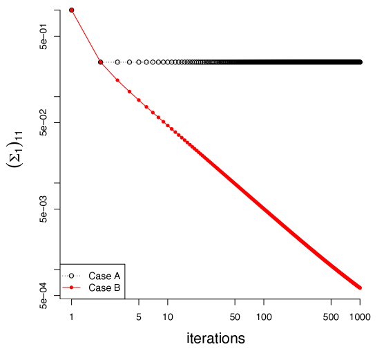
In the runtime experiment (Table II) we define the optimization to be converged when the maximal absolute change in the lambda parameters is $10^{-2}$ or when the maximal change in the means or square roots of variance constraints is at most $10^{-2}$ times the standard deviation of the full data. In the sideR implementation we stop the optimization after c. 10 seconds even if the above conditions are not met. We describe in this section a situation where the time cutoff is typically needed. The iteration is guaranteed to converge eventually, but in certain cases—especially if the dataset ($n$) is small or the size of some clusters ($|I^{t}|$) is small compared to dimensionality ($d$)—the convergence can be slow, as shown in the following adversarial example.

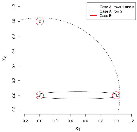
Consider a dataset of three points ($n=3$) and a dimensionality of two ($d=2$), shown in Fig. 5a and given by

$$\hat{\bf X}=\left(\begin{array}[]{cc}1&0\\ 0&1\\ 0&0\end{array}\right),$$ (11)

and two sets of constraints. (A) The first set of constraints are the cluster constraints related to the first and the third row and given by ${\mathcal{C}}_{A}=\{C^{1},\ldots,C^{4}\}$, where $c^{1}=c^{3}=lin$, $c^{2}=c^{4}=quad$, $I^{1}=\ldots=I^{4}=\{1,3\}$, $w^{1}=w^{2}=(1,0)^{T}$, and $w^{3}=w^{4}=(0,1)^{T}$§. (B) The second set of constraints have an additional cluster constraint related to the second and the third row and given by ${\mathcal{C}}_{B}=\{C^{1},\ldots,C^{8}\}$, where $C^{1},\ldots,C^{4}$ are as above and $c^{5}=c^{7}=lin$, $c^{6}=c^{8}=quad$, $I^{5}=\ldots=I^{8}=\{2,3\}$, $w^{5}=w^{6}=(1,0)^{T}$, and $w^{7}=w^{8}=(0,1)^{T}$.

(Case A) The solution to Prob. 1 with constraints in ${\mathcal{C}}_{A}$ is given by ${\bf m}_{1}={\bf m}_{3}=(1/2,0)^{T}$, ${\bf m}_{2}=(0,0)^{T}$,

$$\Sigma_{1}=\Sigma_{3}=\left(\begin{array}[]{cc}1/4&0\\ 0&0\end{array}\right),~{}~{}~{}\mbox{ and }\Sigma_{2}=\left(\begin{array}[]{cc}1&0\\ 0&1\end{array}\right).$$ (12)

Note that if the number of data points in a cluster constraint is at most the number of dimensions in the data there are necessarily directions in which the variance of the background distribution is zero, see Fig. 5a. However, since we have here a single cluster constraint with no overlapping constraints, the convergence is very fast and in fact occurs after one pass over the lambda variables as shown in Fig. 5b (black line).

(Case B) The solution to Prob. 1 with constraints in ${\mathcal{C}}_{B}$ are given by ${\bf m}_{1}=(1,0)^{T}$, ${\bf m}_{2}=(0,1)^{T}$, ${\bf m}_{3}=(0,0)^{T}$, and

$$\Sigma_{1}=\Sigma_{2}=\Sigma_{3}=\left(\begin{array}[]{cc}0&0\\ 0&0\end{array}\right).$$ (13)

Here we observe that adding a second overlapping cluster constraint, combined with the small variance directions in both the constraints restricts the variance of the third data point to zero. Because both of the clusters have only one additional data point it follows that the variance of all data points is zero. The small variance and overlapping data points cause the convergence here to be substantially slower, as shown in Fig. 5b (red line). The variance scales roughly as $(\Sigma_{1})_{11}\propto\tau^{-1}$, where $\tau$ is the number of optimization steps, the global optimum being in singular point at $(\Sigma_{1})_{11}=0$.

The slow convergence is due to overlapping and quadratic constraints with small variance (caused here by small number of points per cluster). A way to speed up the convergence would be—perhaps unintuitively—to add more data points: e.g., to replicate each data point 10 times with random noise added to each replicate. When a data point would be selected to a constraint then all of its replicates would be included as well. This would set a lower limit on the variance of the background model and hence, be expected to speed up the convergence. Another way to solve the issue is just to cut off the iterations after some time point—which is what we do here—leading up to larger variance than in the optimal solution. This appears to be typically acceptable in practice.

II-B Whitening out the background distribution

Once we have found the distribution that solves Prob. 1, the next task is to find and visualize the maximal differences between the data and the background distribution defined by Eq. (5). To this end we sample a dataset from the background distribution, and produce a whitened version of the data.

The random dataset can be obtained by sampling a data point $i\in[n]$ from the multivariate Gaussian distribution parametrized by $\theta_{i}$. The whitening operation is more involved. The direction-preserving whitening transformation of the data results in a unit Gaussian spherical distribution, if the data follows the current background distribution. Thus, any deviation from the unit sphere distribution is a signal of difference between the data and the current background distribution.

More specifically, we define new data vectors $\mathbf{y}_{i}$ as follows,

$$\mathbf{y}_{i}=U_{i}D_{i}^{1/2}U_{i}^{T}\left(\mathbf{x}_{i}-\mathbf{m}_{i}\right),$$ (14)

where the SVD decomposition of $\Sigma_{i}^{-1}$ is given by $\Sigma_{i}^{-1}=U_{i}D_{i}U^{T}_{i}$, where $U_{i}$ is an orthogonal matrix and $D_{i}$ is a diagonal matrix. If we used one transformation matrix for the whole data, this would correspond to the normal whitening transformation. However, here we may have a different transformation for each of the rows. Furthermore, normally the transformation matrix would be computed from the data, but here we compute it from the constrained model.

Figure 7: The full user interface of sideR. The data shown here is the British National Corpus data, see Sec. IV-B for details.

It is easy to see that if $\mathbf{x}_{i}$ obeys the distribution of Eq. (5), then $D_{i}^{1/2}U_{i}^{T}\left(\mathbf{x}_{i}-\mathbf{m}_{i}\right)$ obeys unit spherical distribution. Hence, any rotation of this vector obeys a unit sphere distribution as well. We rotate this vector back to the direction of $x_{i}$ so that after the final rotation, $\mathbf{y}_{i}$ for different rows $i$ have a comparable direction. We use $\hat{\bf Y}=\left(\hat{\bf y}_{1}\hat{\bf y}_{2}\ldots\hat{\bf y}_{n}\right)^{T}$ to denote the whitened data matrix. When there are no constraints ${\bf m}_{i}={\bf 0}$ and $\Sigma_{i}^{-1}={\bf 1}$ and the whitening operation therefore reduces to identity operation, i.e., $\hat{\bf Y}=\hat{\bf X}$.

Example 3.

To illustrate the whitening operation, we show in Fig. 6 pairplots of the whitened data matrix $\hat{\bf Y}_{5}$, for the synthetic data $\hat{\bf X}_{5}$. Initially (Fig. 6a) the whitened data matches $\hat{\bf X}_{5}$. Fig. 6b shows the whitened data after adding a cluster constraint for each of the four clusters in Fig. 4a and updating the background distribution accordingly. Now, in the first three dimensions the whitened data does not anymore significantly differ from Gaussian distribution, while in dimensions 4 and 5 it still does.

II-C PCA and ICA

To find directions where the data and the background distribution differ, i.e., the whitened data $\hat{\bf Y}$ looks different from the unit Gaussian distribution with zero mean, an obvious choice is to use Principal Component Analysis (PCA) and look for directions in which the variance differs most from unity. However, it may happen that the variance is already taken into account in the variance constraints, in which case PCA is not informative because all directions in $\hat{\bf Y}$ have equal mean and variance. Instead, we can for example use Independent Component Analysis (ICA) and the FastICA algorithm [6] with log-cosh $G$ function as a default method to find non-Gaussian directions. Clearly, when there are no constraints, the approach equals standard PCA and ICA on the original data but when there are constraints the output will be different.

Example 4.

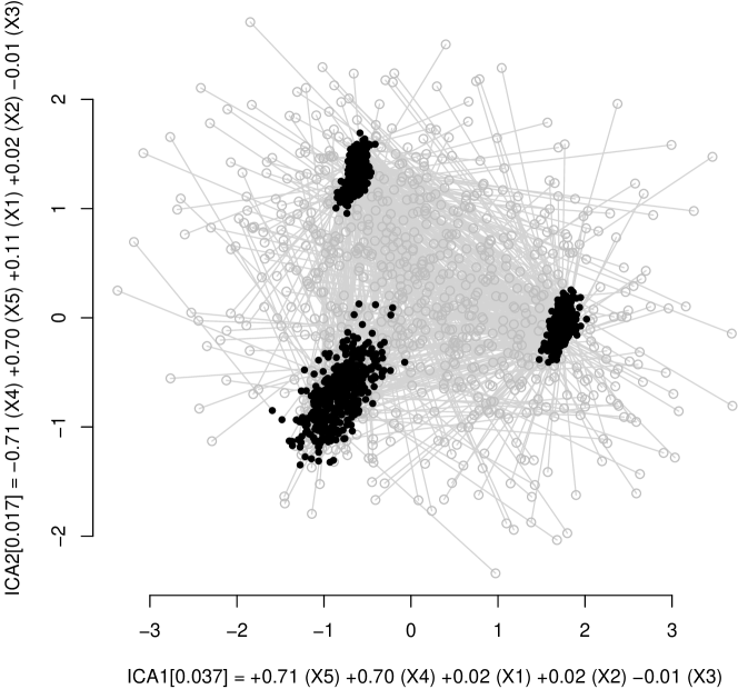
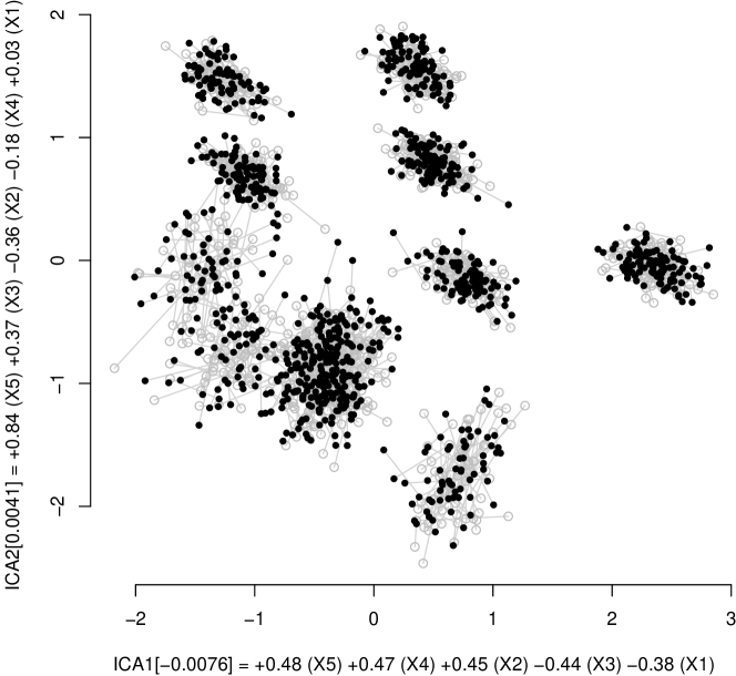
Fig. 4c shows the directions in which the whitened data $\hat{\bf Y}_{5}$ in Fig. 6b differs the most from Gaussian. The user can observe the cluster structure in dimensions 4 and 5, which would not be possible with non-iterative methods. After adding a cluster constraint for each of the three visible clusters, the updated background distribution becomes a faithful representation of the data, and thus the whitened data shown in Fig. 6c resembles a unit Gaussian spherical distribution. This is also reflected in a visible drop in ICA scores in Table I.

III Proof-of-concept system sideR

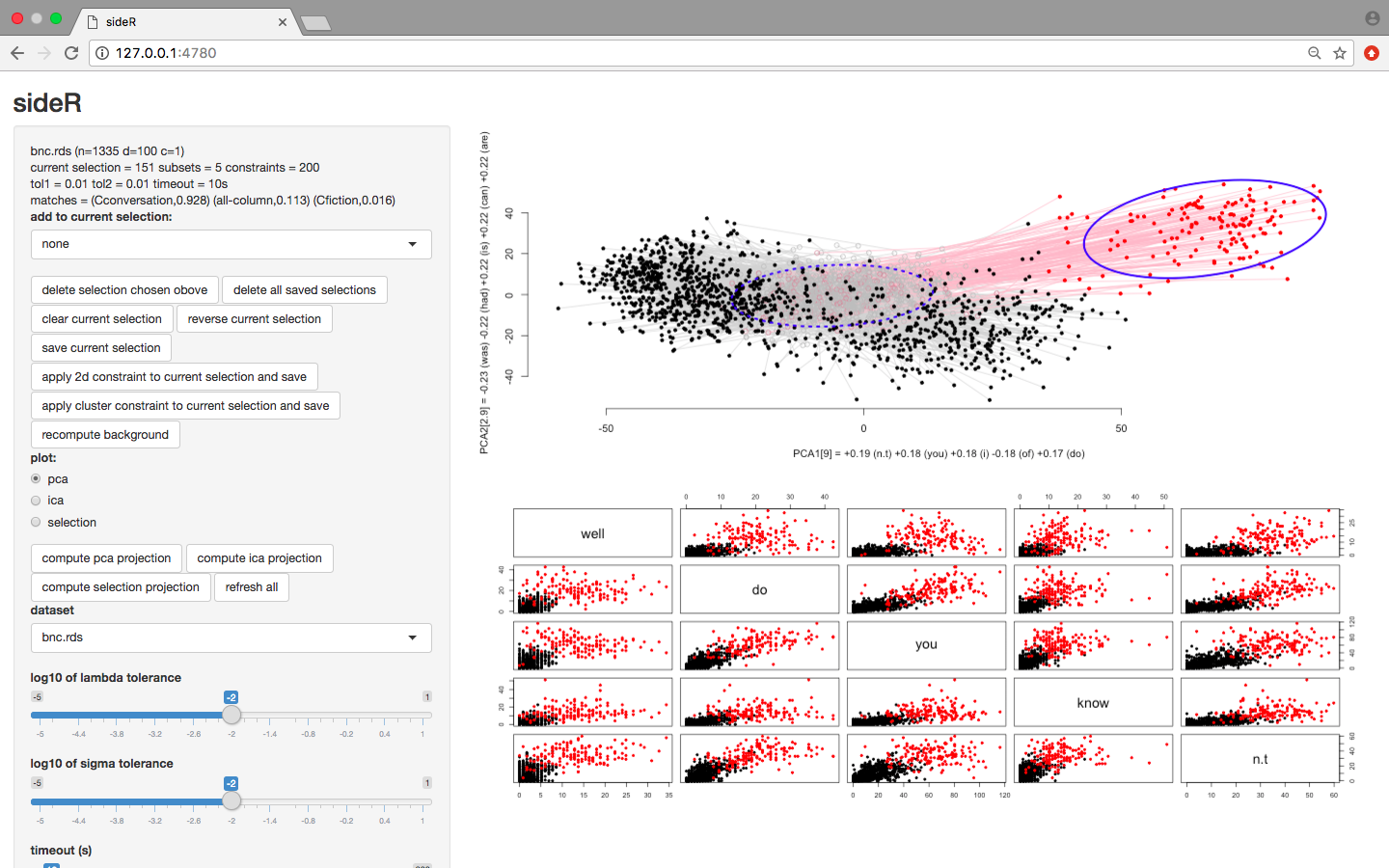
We have implemented the concepts described above in an interactive demonstrator system sideR using R 3.4.0 [7] with shiny [8] and fastICA [9]. sideR runs in the web browser using R as a back-end. The user interface of sideR is shown in Fig. 7. The main scatterplot (upper right corner) shows the PCA (here) or ICA projection of the data to directions in which the data and the background distribution differ most. The data is shown by solid black spheres and the currently selected data by solid red spheres. The sample from the background distribution is shown by gray circles, with a gray line connecting the data points with the corresponding sampled background points. Notice that the gray points and lines only provide a proxy for the difference between the data and the background distribution, since in reality the background distribution has a specified mean and covariance structure for every point. Nonetheless this should illustrate broadly the density structure of the background distribution for the current projection, which we think is helpful to understand why the current visualization may provide new insights.

We also show a pairplot (lower right corner) directly dislaying the attributes maximally different with respect to the current selection (red points) as compared to the full dataset. In the left-hand panel we show some statistics of the full data and of the data points that have been selected. We also show in the main scatterplot (upper right corner) in blue the 95% confidence ellipsoids for the distribution of the selection (solid blue ellipsoid) and the respective background samples (dotted blue ellipsoid) to aid in figuring out if the location of the selected points in the current projection differs substantially from the expected location under the background distribution.

The user can add data points to a selection by directly marking them, by using pre-defined classes that exist in the dataset, or previously saved groupings. The user can create a 2-D or cluster constraint of the current selection by clicking the appropriate button on the left-hand panel as well as recompute the background distribution to match the current constraints and update the projections. The user can also adjust convergence parameters which have by default been set so that the maximal time taken to update the background distribution is $\sim$10 seconds which is in practice typically more than enough. The interface has been designed so that time-consuming operations (taking more than $\sim$2 seconds, i.e., the updating the background distribution or computing the ICA projection) are executed only by a direct command by the user, which makes the system responsive and predictable.

IV Experiments

In this section we demonstrate the use of our method and the tool sideR. Our focus here is to show how the tool is able to provide the user with insightful projections of data and reveal the differences between the background distribution and the data. Additionally, the user interface makes it easy to explore various statistics and properties of selections of data points.

We start by a runtime experiment in which we test the system with data set sizes typical for interactive systems, i.e., there are on the order of thousands of data points; if there are more data points it often makes sense to downsample the data first. Then we use real datasets to illustrate how the system is able to find relevant projections for the user and display differences between the background distribution and the data.

IV-A Runtime experiment

We generated synthetic datasets parametrized by the number of data points ($n$), dimensionality of the data ($d$), and the number of clusters ($k$). Each dataset was created by first randomly sampling $k$ cluster centroids and then allocating data points around each of the centroids. We added column constraints ($2d$ constraints) for each dataset and for the datasets with $k>1$ we additionally used cluster constraints for each of the $k$ clusters in the data ($2dk$ constraints). In Table II the median wall clock running times are provided without any cut-off, based on 10 runs for each set of parameters, ran on a Apple MacBook Air with 2.2 GHz Intel Core i7 processor and a single-threaded R 3.4.0 implementation of the algorithm.

The algorithm is first initialized (init) which is typically very fast, after which the correct parameters are found (optim). Then preprocessing is done for sampling and whitening (preprocess) after which we produce a whitened dataset (whitening) and a random sample of the maxent distribution (sample). These are then used to run the PCA (pca) and ICA (ica) algorithms. We found that init, preprocess, whitening, sample, and pca always take less than 2 seconds each and they are not reported in the table. Most of the time is consumed by optim. We observe in Table II that, as expected, the time consumed does not depend on the number of rows $n$ in the dataset. Each of the optimization steps takes $O(d^{2})$ time per constraint and there are $O(kd)$ constraints, hence the time consumed scales as expected roughly as $O(kd^{3})$. In sideR the default setting is to stop the optimization after a time cut-off of 10 seconds, even when convergence has not been achieved. For larger matrices the time consumed by ICA becomes significant, scaling roughly as $O(nd^{2})$.

TABLE II: Median wall clock running times, based on 10 runs for each set of parameters for finding the correct parameters (optim) and running the ICA (ica) algorithm without time cutoff.

		seconds, $k\in\{1,2,4,8\}$
$n$	$d$	optim	ica
$2048$	$16$	$\{0.0,0.2,0.3,0.5\}$	$\{0.6,0.6,0.6,0.6\}$
$2048$	$32$	$\{0.0,0.6,1.0,2.1\}$	$\{1.5,1.5,1.6,1.6\}$
$2048$	$64$	$\{0.1,2.7,5.2,11.0\}$	$\{5.1,5.2,4.9,4.9\}$
$2048$	$128$	$\{1.2,21.4,48.1,124.6\}$	$\{17.8,17.6,17.4,17.0\}$
$4096$	$16$	$\{0.0,0.2,0.3,0.5\}$	$\{1.1,1.1,1.1,1.1\}$
$4096$	$32$	$\{0.0,0.6,1.0,2.0\}$	$\{3.1,3.4,3.0,3.1\}$
$4096$	$64$	$\{0.2,2.5,6.0,11.6\}$	$\{9.8,9.3,9.5,9.6\}$
$4096$	$128$	$\{1.2,23.4,56.4,121.3\}$	$\{34.2,34.7,34.4,34.4\}$
$8192$	$16$	$\{0.0,0.2,0.3,0.6\}$	$\{2.6,2.2,2.5,2.1\}$
$8192$	$32$	$\{0.0,0.6,1.0,2.0\}$	$\{6.5,6.0,5.9,5.9\}$
$8192$	$64$	$\{0.2,2.7,6.0,12.2\}$	$\{20.7,20.4,19.8,20.1\}$
$8192$	$128$	$\{1.2,21.9,44.1,110.3\}$	$\{67.9,67.5,67.1,67.6\}$

(a)	(b)

Figure 8: A use case with the BNC data. (a) Selection of points for the second cluster constraint. The view is the next most informative PCA projection obtained after adding a cluster constraint for the points selected in Fig. 7 and updating of the background distribution. (b) After adding a cluster constraint again and updating of the background distribution, there is no longer a striking difference between the background distribution and the data in the PCA projection.

IV-B British National Corpus data

The British National Corpus (BNC) [10] is one of the largest annotated text corpora freely available in full-text format. The texts are annotated with information such as author gender, age, and target audience, and all texts have been classified into genres [11]. As a high dimensional use case we explore the high-level structure of the corpus. For a preprocessing step, we compute the vector-space model (word counts) using the first 2000 words from each text belonging to one the four main genres in the corpus (‘prose fiction’, ‘transcribed conversations’, ‘broadsheet newspaper’, ‘academic prose’) as done in [12]. After preprocessing we have word counts for 1335 texts and we use the 100 words with highest counts as the dimensions and the main genres as the class information.

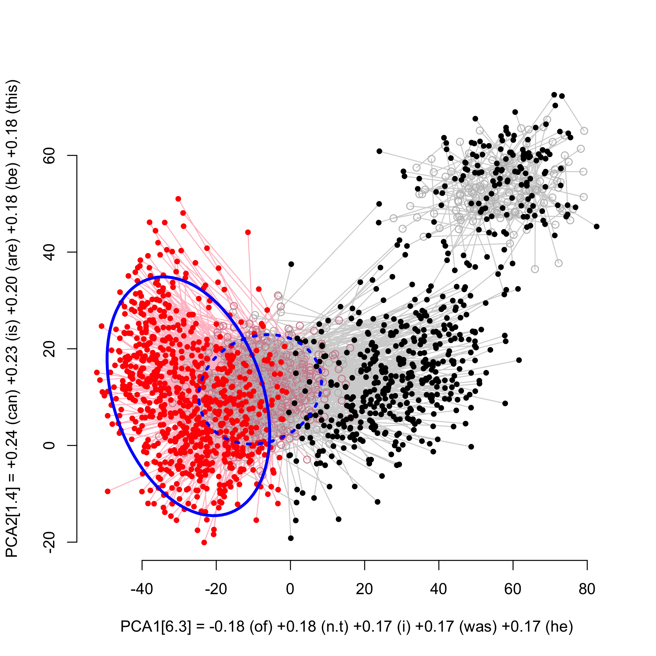
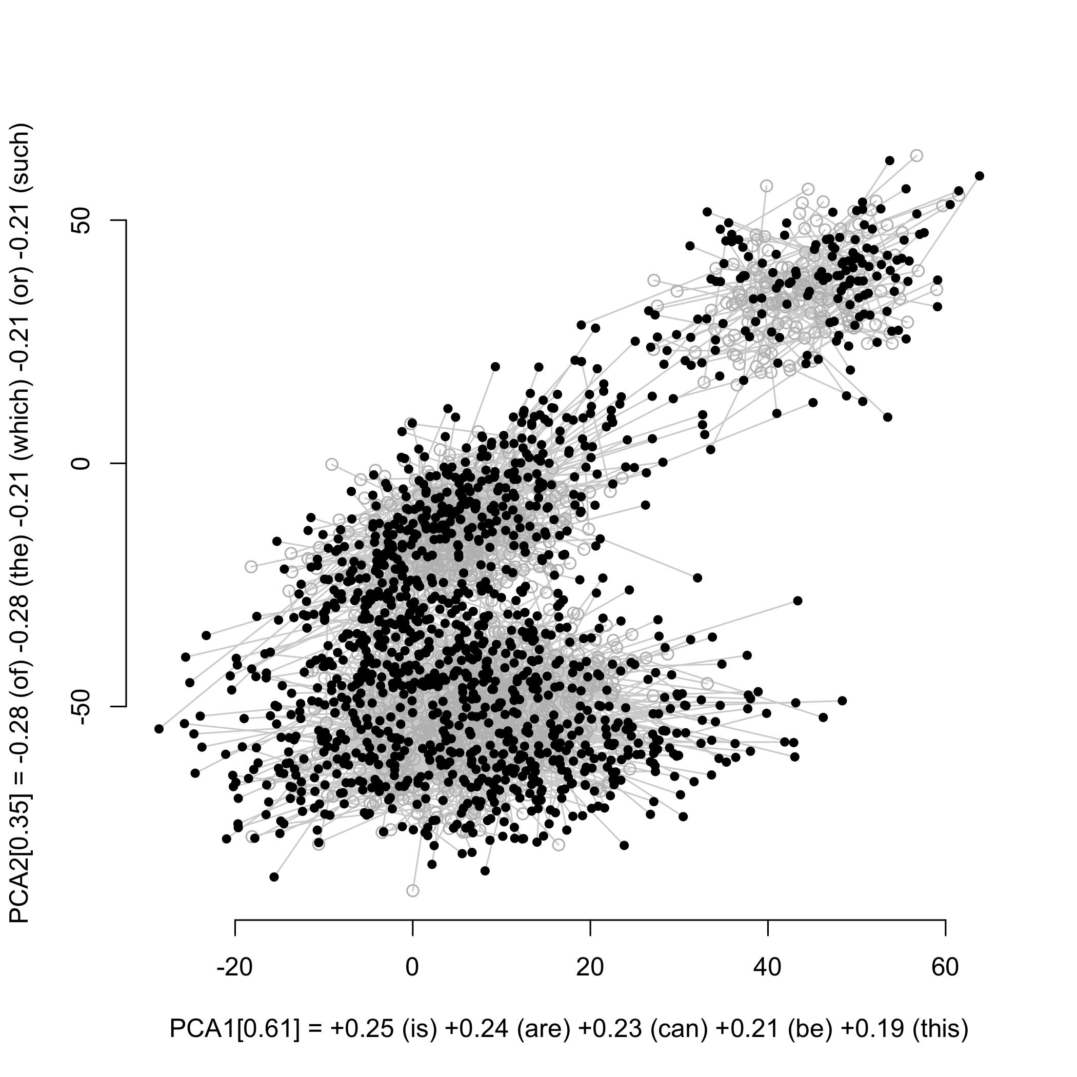
The most informative PCA projection to the BNC data is shown in Fig. 7. In the upper right corner there is a group of points (red selection) that appear to form a group. The selected points are mainly texts from ‘transcribed conversations’ (Jaccard-index to class 0.928), and the pairplot in Fig. 7 (lower right) shows the selection of points differing from the rest of the data. After we added a cluster constraint for this selection, updated the background distribution and computed a new PCA projection, we obtained the projection in Fig. 8a.

The next selection shows another set of points differing from the background distribution. This set of points mainly contains ‘academic prose’ and ‘broadsheet newspaper’ (Jaccard-indices 0.63 and 0.35). After adding a cluster constraint for this selection, we updated the background distribution and computed another PCA projection, resulting in the projection in Fig. 8b. Now, there is no apparent difference to the background distribution (reflected indeed in low PCA scores), and we conclude that the identified ‘prose fiction’ class, together with the combined cluster of ‘academic prose’ and ‘broadsheet newspaper’ explain the data well wrt. variation in counts of the most frequent words. Notice that we did not provide the class labels in advance, they were only used retrospectively.

Figure 9: A use case with the UCI Image Segmentation data. (a) The first view shows that initially the scale of background distribution significantly differs from that of the data. (b) After adding a 1-cluster constraint and performing an update of the background distribution there is visible structure present. The points selected for the first cluster constraint are shown in red. (c) and (d) The selections of points for the second and third cluster constraint, respectively. (e) After three cluster constraints are added and the background distribution is updated accordingly, the data and the background distribution are similar in this projection. (f) The next PCA projection shows mainly outliers.

IV-C UCI Image Segmentation data

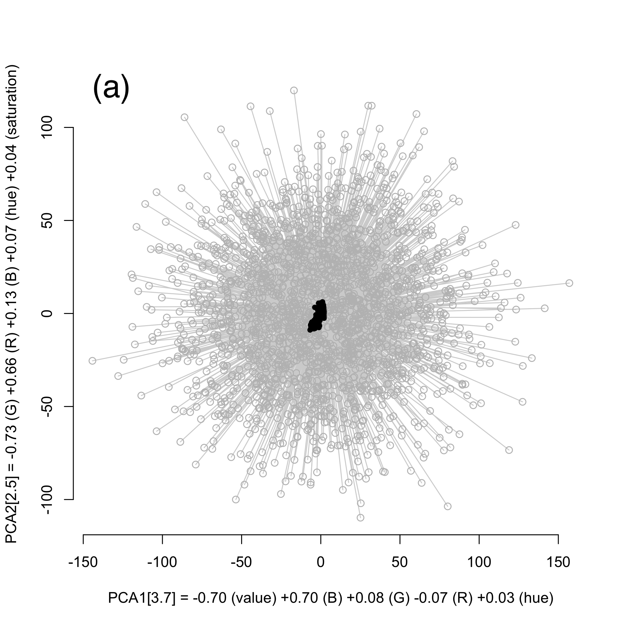
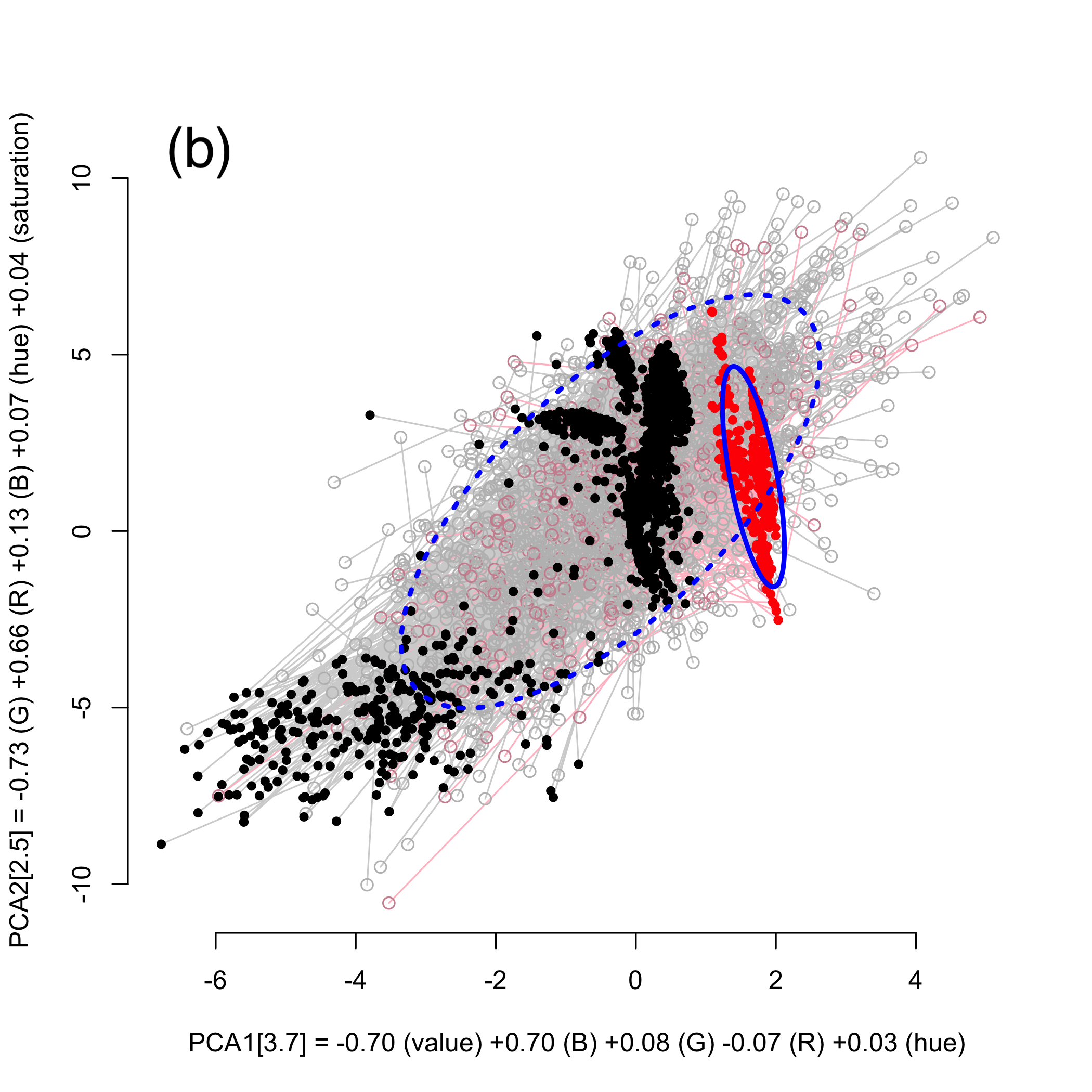
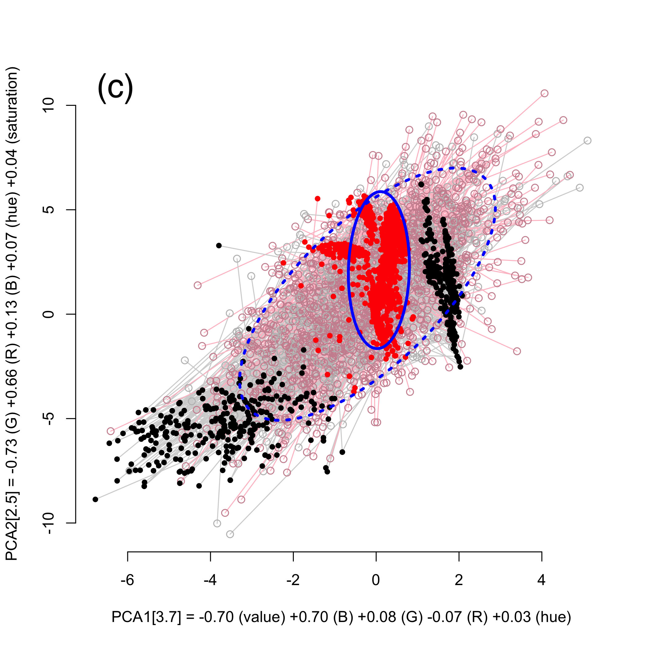
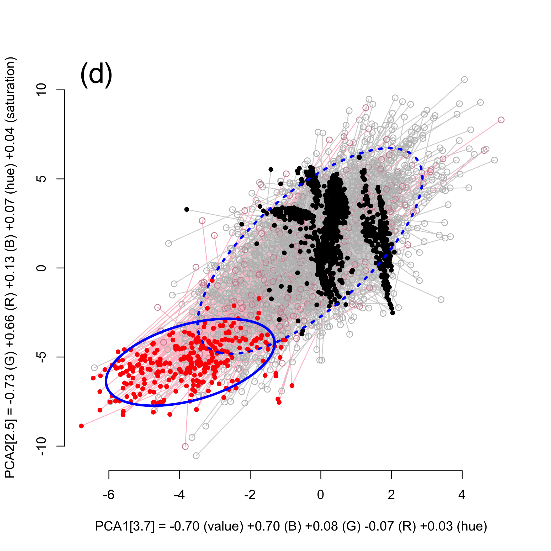
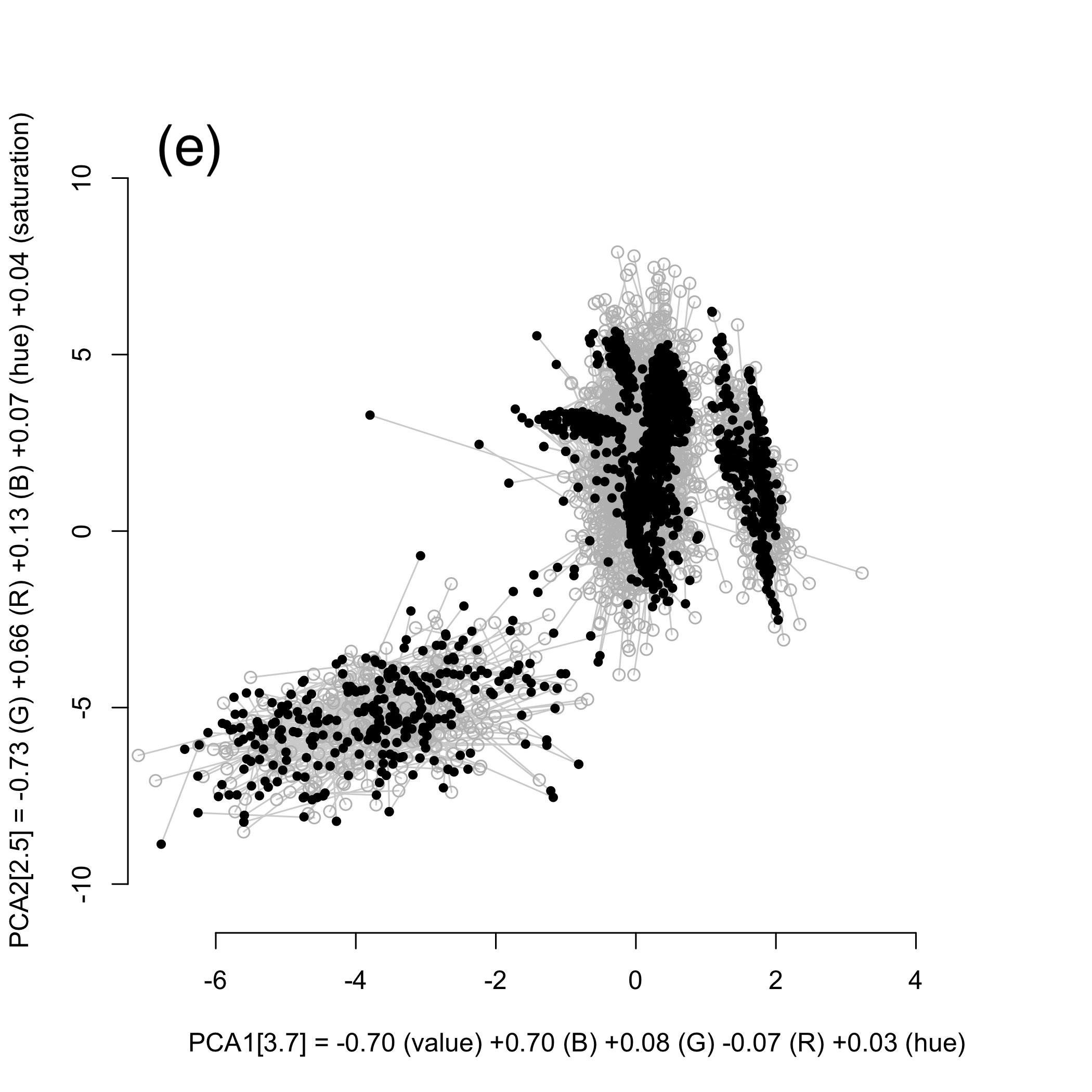
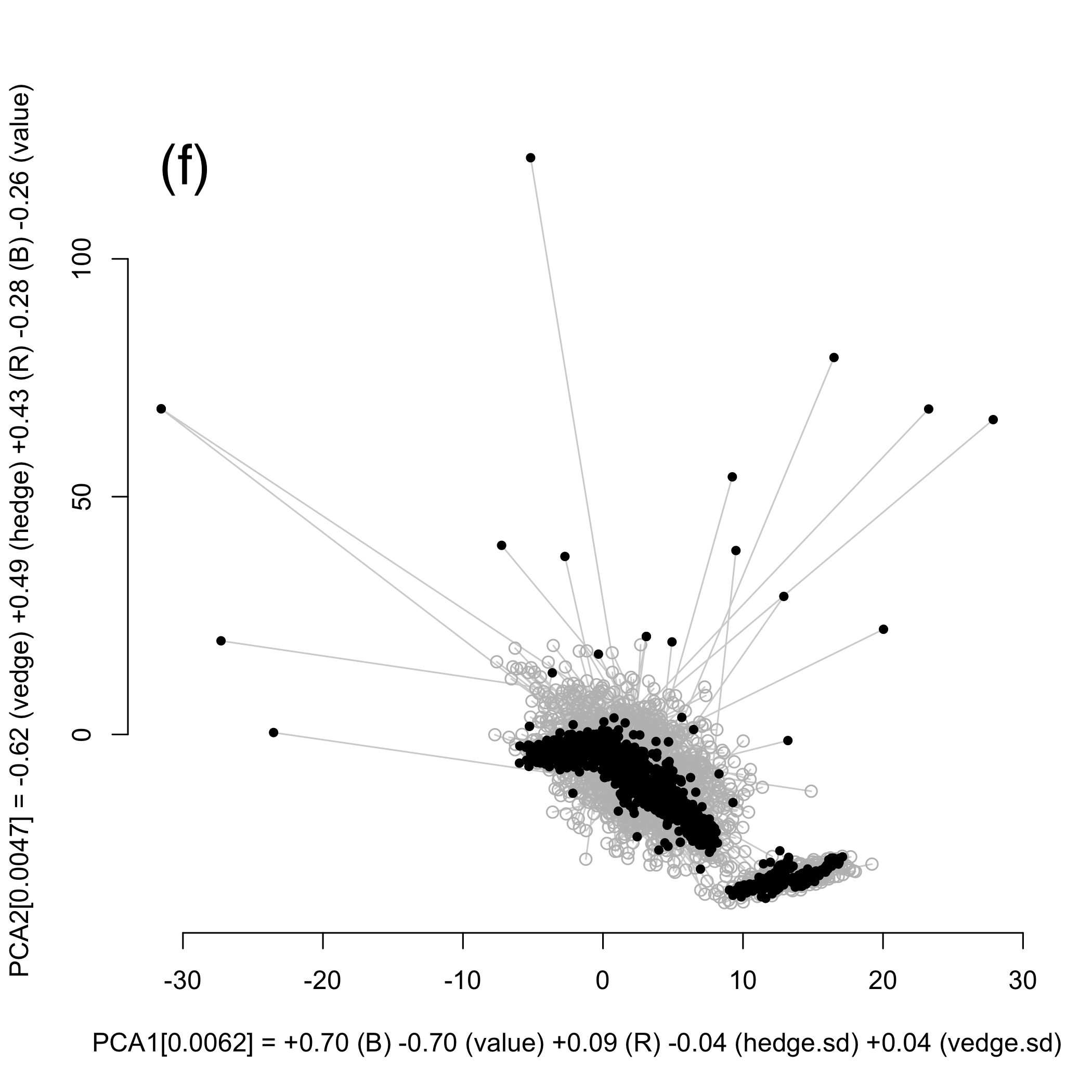
As a second use case, we have the Image Segmentation dataset from the UCI machine learning repository [13] with 2310 samples. The PCA projection (Fig. 9a) shows that the background distribution has a much larger variance than the data. Thus, we first added a 1-cluster constraint for the data (overall covariance) and updated the background distribution. After this (Fig. 9b) $\geq 3$ sets of points quite clearly separated in the projection can be observed. The set of 330 points selected in Fig. 9b contains solely points from the class ‘sky’, while the 316 points in the lower left corner (selected in Fig. 9d) are mainly from the class ‘grass’ (with Jaccard-index 0.964). The set of points clustered in the middle (selected in Fig. 9c) are mainly from classes ‘brickface’, ‘cement’, ‘foliage’, ‘path’, and ‘window’ (with Jaccard-index approx. 0.2 each). We add a cluster constraint for each of selection, and show the updated background distribution in Fig. 9e. We can observe that the background distribution now matches the data rather well with the exception of some outliers. The next PCA projection (Fig. 9f) reveals that indeed there are outliers. For brevity, we did not continue the analysis, but the data obviously contains a lot more structure that we could explore in subsequent iterations. Furthermore, in many applications identifying and studying the outlier points deviating from the three-cluster main structure of the data could be interesting and useful.

V Related Work

This work is motivated by the ideas in [14] in which a similar system was constructed using constrained randomization. The constrained randomization approach [15, 16] is similar to the Maximum Entropy distribution used here, but it relies on sampling of the data and no direct distribution assumptions are made. An advantage of the approach taken here is that it is faster—which is essential in interactive applications—and scales more easily to large data. Furthermore, here we have an explicit analytic form for the background distribution unlike in [14], where the background distribution was defined by a permutation operation. The mathematical form of linear and quadratic constraints and efficient inference of the background distribution has been developed by us in [4]. The presentation here is new and non-overlapping. The analytic form of the background distribution allows us, in addition to speeding up the computations, to define interestingness functions and the cluster constraint in a more natural manner. Here we also introduce the whitening method that allows our approach to be used with standard and robust projection pursuit methods such as PCA or ICA instead of the tailor-made line search algorithm of [14]. Furthermore, we provide a fluent open source implementation written in R.

The Maximum Entropy method has been proposed as a part of Formalizing Subjective Interestingess (forsied) framework of data mining [17, 18] modelling the user’s knowledge by a background distribution. forsied has been studied in the context of dimensionality reduction and EDA [19, 20]. To the best of our knowledge, ours is the first instance in which this background distribution can be updated by a direct interaction of the user, thus providing a principled method of EDA.

Many other special-purpose methods have been developed for active learning in diverse settings, e.g., in classification and ranking, as well as explicit models for user preferences. However, as these approaches are not targeted at data exploration, we do not review them here. Finally, several special-purpose methods have been developed for visual iterative data exploration in specific contexts, e.g., for itemset mining and subgroup discovery [21, 22, 23, 24], information retrieval [25], and network analysis [26].

The system presented here can be also considered to be an instance of visually controllable data mining [27], where the objective is to implement advanced data analysis methods understandable and efficiently controllable by the user. Our approach satisfies the properties of a visually controllable data mining method (see [27], Sec. II B): (VC1) the data and model space are presented visually, (VC2) there are intuitive visual interactions allowing the user to modify the model space, and (VC3) the method is fast enough for visual interaction.

Dimensionality reduction for EDA has been studied for decades starting with multidimensional scaling (MDS) [28, 29] and projection pursuit [2, 3]. Recent research on this topic (referred to as manifold learning) is still inspired by MDS: find a low-dimensional embedding of points representing well the the distances in the high-dimensional space. In contrast to PCA [30], the idea is to preserve small distances, and large distances are irrelevant, as long as they remain large, e.g., Local Linear and (t-)Stochastic Neighbor Embedding [31, 32, 33]. This is typically not possible to achieve perfectly, and a trade-off between precision and recall arises [34].

Many new interactive visualization methods are presented yearly at the IEEE VIS Conference. The focus there is not on the use or development of new data mining or machine learning techniques, but rather on human cognition, efficient use of displays, and exploration via data object and feature selection. Yet, there is a growing interest and potential synergies with data mining were already recognized long ago [35].

VI Conclusions

There have been many efforts in analysis of multivariate data in different contexts. For example, there are several Projection Pursuit and manifold learning methods for using some criteria to compress the data into a lower dimensional—typically 2-D—presentation while preserving features of interest. The inherent drawback of this approach is that the criteria for dimensionality reduction are defined typically in advance and it may or may not fit the user’s need. It may be that a visualization shows only the most prominent features of the data already known for the user, or features that are irrelevant for the task at hand.

The advantage of the dimensionality reduction methods is that the computer, unlike the human user, has a “view” of all the data and it can select a view in a more fine-tuned way and by using a more complex criteria than a human could. A natural alternative to static visualizations using pre-defined criteria is the addition of interaction. The drawback of such interactions is, however, that they lack the sheer computational power utilized by the dimensionality reduction methods.

Our method fills the gap between automated dimensionality reduction methods and interactive systems. We propose to model the knowledge of a domain expert by a probability distribution computed by using the Maximum Entropy criteria. Furthermore, we propose powerful and yet intuitive interactions for the user to update the background distribution. Our approach uses Projection Pursuit methods and shows the directions in which the data and the background distribution differ the most. In this way, we utilize the power of Projection Pursuit at the same the allowing the user to adjust the criteria by which the computers chooses the directions to show her.

The current work presents a framework and a system for real-valued data and the background distribution which is modeled by multivariate Gaussian distributions. The same ideas could be generalized to other data types, such as categorical or ordinal data values, or to higher-order statistics, likely in a straightforward manner, as the mathematics of exponential family distribution would lead to similar derivations.

Our approach could also be extended to other interactions especially in knowledge intensive tasks. Instead of designing interactions directly and explicitly we can think that the “views of the data” (here mainly 2-D projections) and the interactions (here, e.g., marking the constraints) could also in other contexts be modeled as operations modifying the user’s “background model”. One of the main benefits of our approach is that the user marks the patterns she observes and thus the background distribution is always customized to the user’s understanding of the data, without a need for assumptions such as that high variance directions are interesting to everyone, as implicitly assumed when applying PCA for visualization.

For concrete applications for our approach and the sideR tool there is potential in, e.g., computational flow cytometry. Initial experiments with samples up to tens of thousands rows from flow-cytometry data [36] has shown the computations in sideR to scale up well and the projections to reveal structure in the data potentially interesting to the application specialist.

Acknowledgements. This work has been supported by the ERC under the EU’s Seventh Framework Programme (FP/2007- 2013) / ERC Grant Agreement no. 615517, the FWO (project no. G091017N, G0F9816N), the EU’s Horizon 2020 research and innovation programme and the FWO under the MSC Grant Agreement no. 665501, the Academy of Finland (decision 288814), and Tekes (Revolution of Knowledge Work project).

References

- [1] J. Tukey, Exploratory data analysis. Reading, Mass.: Addison-Wesley, 1977.
- [2] J. Friedman and J. Tukey, “A projection pursuit algorithm for exploratory data analysis,” IEEE T. Comp., vol. 100, no. 23, pp. 881–890, 1974.
- [3] P. Huber, “Projection pursuit,” Ann. Stat., vol. 13, no. 2, pp. 435–475, 1985.
- [4] J. Lijffijt, B. Kang, W. Duivesteijn, K. Puolamäki, E. Oikarinen, and T. De Bie, “Subjectively interesting subgroup discovery on real-valued targets,” arXiv:1710.04521 [stat.ML], 2017.
- [5] T. Cover and J. Thomas, Elements of Information Theory, 2nd ed. Wiley, 2005.
- [6] A. Hyvärinen, “Fast and robust fixed-point algorithms for independent component analysis,” IEEE T. Neural Networ., vol. 10, no. 3, pp. 626–634, 1999.
- [7] R Core Team, R: A Language and Environment for Statistical Computing, R Foundation for Statistical Computing, Austria, 2017. [Online]. Available: https://www.R-project.org/
- [8] W. Chang, J. Cheng, J. Allaire, Y. Xie, and J. McPherson, shiny: Web Application Framework for R, 2017, r package version 1.0.3. [Online]. Available: https://CRAN.R-project.org/package=shiny
- [9] J. Marchini, C. Heaton, and B. Ripley, fastICA: FastICA Algorithms to perform ICA and Projection Pursuit, 2013, r package version 1.2-0. [Online]. Available: https://CRAN.R-project.org/package=fastICA
- [10] “The British National Corpus, v. 3 (BNC XML Edition),” Distributed by Oxford University Computing Services on behalf of the BNC Consortium, 2007. [Online]. Available: http://www.natcorp.ox.ac.uk/
- [11] D. W. Lee, “Genres, registers, text types, domain, and styles: Clarifying the concepts and navigating a path through the BNC jungle.” Language Learning & Technology, vol. 5, no. 3, pp. 37–72, 2001.
- [12] J. Lijffijt and T. Nevalainen, “A simple model for recognizing core genres in the BNC,” Studies in Variation, Contacts and Change in English, Forthcoming.
- [13] M. Lichman, “UCI machine learning repository,” 2013. [Online]. Available: http://archive.ics.uci.edu/ml
- [14] K. Puolamäki, B. Kang, J. Lijffijt, and T. De Bie, “Interactive visual data exploration with subjective feedback,” in Proc. of ECML-PKDD, 2016, pp. 214–229.
- [15] S. Hanhijärvi, M. Ojala, N. Vuokko, K. Puolamäki, N. Tatti, and H. Mannila, “Tell me something I don’t know: Randomization strategies for iterative data mining,” in Proc. of KDD, 2009, pp. 379–388.
- [16] J. Lijffijt, P. Papapetrou, and K. Puolamäki, “A statistical significance testing approach to mining the most informative set of patterns,” DMKD, vol. 28, no. 1, pp. 238–263, 2014.
- [17] T. De Bie, “An information-theoretic framework for data mining,” in Proc. of KDD, 2011, pp. 564–572.
- [18] ——, “Subjective interestingness in exploratory data mining,” in Proc. of IDA, 2013, pp. 19–31.
- [19] T. De Bie, J. Lijffijt, R. Santos-Rodriguez, and B. Kang, “Informative data projections: a framework and two examples,” in Proc. of ESANN, 2016, pp. 635 – 640.
- [20] B. Kang, J. Lijffijt, R. Santos-Rodríguez, and T. De Bie, “Subjectively interesting component analysis: Data projections that contrast with prior expectations,” in Proc. of KDD, 2016, pp. 1615–1624.
- [21] M. Boley, M. Mampaey, B. Kang, P. Tokmakov, and S. Wrobel, “One click mining—interactive local pattern discovery through implicit preference and performance learning,” in Proc. of KDD IDEA, 2013, pp. 27–35.
- [22] V. Dzyuba and M. van Leeuwen, “Interactive discovery of interesting subgroup sets,” in Proc. of IDA, 2013, pp. 150–161.
- [23] M. van Leeuwen and L. Cardinaels, “Viper — visual pattern explorer,” in Proc. of ECML–PKDD, 2015, pp. 333–336.
- [24] D. Paurat, R. Garnett, and T. Gärtner, “Interactive exploration of larger pattern collections: A case study on a cocktail dataset,” in Proc. of KDD IDEA, 2014, pp. 98–106.
- [25] T. Ruotsalo, G. Jacucci, P. Myllymäki, , and S. Kaski, “Interactive intent modeling: Information discovery beyond search,” CACM, vol. 58, no. 1, pp. 86–92, 2015.
- [26] D. Chau, A. Kittur, J. Hong, and C. Faloutsos, “Apolo: making sense of large network data by combining rich user interaction and machine learning,” in Proc. of CHI, 2011, pp. 167–176.
- [27] K. Puolamäki, P. Papapetrou, and J. Lijffijt, “Visually controllable data mining methods,” in Proc. of ICDMW, 2010, pp. 409–417.
- [28] J. B. Kruskal, “Nonmetric multidimensional scaling: A numerical method,” Psychometrika, vol. 29, no. 2, pp. 115–129, 1964.
- [29] W. Torgerson, “Multidimensional scaling: I. theory and method,” Psychometrika, vol. 17, no. 4, pp. 401–419, 1952.
- [30] K. Pearson, “On lines and planes of closest fit to systems of points in space,” Philosophical Magazine, vol. 2, no. 11, pp. 559–572, 1901.
- [31] G. Hinton and S. Roweis, “Stochastic neighbor embedding,” in Proc. of NIPS, 2003, pp. 857–864.
- [32] S. Roweis and L. Saul, “Nonlinear dimensionality reduction by locally linear embedding,” Science, vol. 290, no. 5500, pp. 2323–2326, 2000.
- [33] L. van der Maaten and G. Hinton, “Visualizing data using t-SNE,” JMLR, vol. 9, pp. 2579–2605, 2008.
- [34] J. Venna, J. Peltonen, K. Nybo, H. Aidos, and S. Kaski, “Information retrieval perspective to nonlinear dimensionality reduction for data visualization,” JMLR, vol. 11, pp. 451–490, 2010.
- [35] D. Keim, J. Kohlhammer, G. Ellis, and F. Mansmann, Eds., Mastering the Information Age: Solving Problems with Visual Analytics. EG Association, 2010.
- [36] Y. Saeys, S. Van Gassen, and B. Lambrecht, “Computational flow cytometry: helping to make sense of high-dimensional immunology data,” Nat. Rev. Immunol., vol. 16, no. 7, pp. 449–462, 2016.