Fast MCMC Sampling Algorithms on Polytopes

Abstract

We propose and analyze two new MCMC sampling algorithms, the Vaidya walk and the John walk, for generating samples from the uniform distribution over a polytope. Both random walks are sampling algorithms derived from interior point methods. The former is based on volumetric-logarithmic barrier introduced by Vaidya whereas the latter uses John’s ellipsoids. We show that the Vaidya walk mixes in significantly fewer steps than the logarithmic-barrier based Dikin walk studied in past work. For a polytope in ^d defined by $n>d$ linear constraints, we show that the mixing time from a warm start is bounded as $\mathcal{O}\left(n^{0.5}d^{1.5}\right)$, compared to the $\mathcal{O}\left(nd\right)$ mixing time bound for the Dikin walk. The cost of each step of the Vaidya walk is of the same order as the Dikin walk, and at most twice as large in terms of constant pre-factors. For the John walk, we prove an $\mathcal{O}\left(d^{2.5}\cdot\log^{4}(n/d)\right)$ bound on its mixing time and conjecture that an improved variant of it could achieve a mixing time of $\mathcal{O}\left(d^{2}\cdot\text{poly-log}(n/d)\right)$. Additionally, we propose variants of the Vaidya and John walks that mix in polynomial time from a deterministic starting point. The speed-up of the Vaidya walk over the Dikin walk are illustrated in numerical examples.

Keywords: MCMC methods, interior point methods, polytopes, sampling from convex sets

1 Introduction

Sampling from distributions is a core problem in statistics, probability, operations research, and other areas involving stochastic models (Geman and Geman, 1984; Brémaud, 1991; Ripley, 2009; Hastings, 1970). Sampling algorithms are a prerequisite for applying Monte Carlo methods to order to approximate expectations and other integrals. Recent decades have witnessed great success of Markov Chain Monte Carlo (MCMC) algorithms; for instance, see the handbook by Brooks et al. (2011) and references therein. These methods are based on constructing a Markov chain whose stationary distribution is equal to the target distribution, and then drawing samples by simulating the chain for a certain number of steps. An advantage of MCMC algorithms is that they only require knowledge of the target density up to a proportionality constant. However, the theoretical understanding of MCMC algorithms used in practice is far from complete. In particular, a general challenge is to bound the mixing time of a given MCMC algorithm, meaning the number of iterations—as a function of the error tolerance $\delta$, problem dimension $d$ and other parameters—for the chain to arrive at a distribution within distance $\delta$ of the target.

In this paper, we study a certain class of MCMC algorithms designed for the problem of drawing samples from the uniform distribution over a polytope. The polytope is specified in the form $\mathcal{K}:=\{x\in{}^{d}\mid Ax\leq b\}$, parameterized by the matrix-vector pair $(A,b)\in{}^{n\times d}\times{}^{n}$. Our goal is to understand the mixing time for obtaining $\delta$-accurate samples, and how it grows as a function of the pair $\left(n,d\right)$.

The problem of sampling uniformly from a polytope is important in various applications and methodologies. For instance, it underlies various methods for computing randomized approximations to polytope volumes. There is a long line of work on sampling methods being used to obtain randomized approximations to the volumes of polytopes and other convex bodies (see, e.g., Lovász and Simonovits, 1990; Lawrence, 1991; Bélisle et al., 1993; Lovász, 1999; Cousins and Vempala, 2014). Polytope sampling is also useful in developing fast randomized algorithms for convex optimization (Bertsimas and Vempala, 2004) and sampling contingency tables (Kannan and Narayanan, 2012), as well as in randomized methods for approximately solving mixed integer convex programs (Huang and Mehrotra, 2013, 2015). Sampling from polytopes is also related to simulations of the hard-disk model in statistical physics (Kapfer and Krauth, 2013), as well as to simulations of error events for linear programming in communication (Feldman et al., 2005).

Many MCMC algorithms have been studied for sampling from polytopes, and more generally, from convex bodies. Some early examples include the Ball Walk (Lovász and Simonovits, 1990) and the hit-and-run algorithm (Bélisle et al., 1993; Lovász, 1999), which apply to sampling from general convex bodies. Although these algorithms can be applied to polytopes, they do not exploit any special structure of the problem. In contrast, the Dikin walk introduced by Kannan and Narayanan (2012) is specialized to polytopes, and thus can achieve faster convergence rates than generic algorithms. The Dikin walk was the first sampling algorithm based on a connection to interior point methods for solving linear programs. More specifically, as we discuss in detail below, it constructs proposal distributions based on the standard logarithmic barrier for a polytope. In a later paper, Narayanan (2016) extended the Dikin walk to general convex sets equipped with self-concordant barriers.

For a polytope defined by $n$ constraints, Kannan and Narayanan (2012) proved an upper bound on the mixing time of the Dikin walk that scales linearly with $n$. In many applications, the number of constraints $n$ can be much larger than the number of variables $d$. For example, we could imagine one using many hyperplane constraints to approximate complicated convex sets such as sphere or ellipsoid. For such problems, linear dependence on the number of constraints is not desirable. Consequently, it is natural to ask if it is possible to design a sampling algorithm whose mixing time scales in a sub-linear manner with the number of constraints. Our main contribution is to investigate and answer this question in affirmative—in particular, by designing and analyzing two sampling algorithms with provably faster convergence rates than the the Dikin walk while retaining its advantages over the ball walk and the hit-and-run methods.

Our contributions:

We introduce and analyze a new random walk, which we refer to as the Vaidya walk since it is based on the volumetric-logarithmic barrier introduced by Vaidya (1989). We show that for a polytope in ^d defined by $n$-constraints, the Vaidya walk mixes in $\mathcal{O}\left(n^{1/2}d^{3/2}\right)$ steps, whereas the Dikin walk (Kannan and Narayanan, 2012) has mixing time bounded as $\mathcal{O}\left(nd\right)$. So the Vaidya walk is better in the regime $n\gg d$. We also propose the John walk, which is based on the John ellipsoidal algorithm in optimization. We show that the John walk has a mixing time of $\mathcal{O}\left(d^{2.5}\cdot\log^{4}(n/d)\right)$ and conjecture that a variant of it could achieve $\mathcal{O}\left(d^{2}\cdot\text{poly-log}(n/d)\right)$ mixing time. We show that when compared to the Dikin walk, the per-iteration computational complexities of the Vaidya walk and the John walk are within a constant factor and a poly-logarithmic in $n/d$ factor respectively. Thus, in the regime $n\gg d$, the overall upper bound on the complexity of generating an approximately uniform sample follows the order Dikin walk $\gg$ Vaidya walk $\gg$ John walk.

The remainder of the paper is organized as follows. In Section 2, we discuss many polynomial-time random walks on convex sets and polytopes, and motivate the starting point for the new random walks. In Section 3, we introduce the new random walks and state bounds on their rates of convergence and provide a sketch of the proof in Section 3.5. We discuss the computational complexity of the different random walks and demonstrate the contrast between the random walks for several illustrative examples in Section 4. We present the proof of the mixing time for the Vaidya walk in Section 5 and defer the analysis of the John walk to the appendix. We conclude with possible extensions of our work in Section 6.

Notation:

For two sequences $a_{\delta}$ and $b_{\delta}$ indexed by $\delta\in I\subseteq\real$, we say that $a_{\delta}=\mathcal{O}\left(b_{\delta}\right)$ if there exists a universal constant $C>0$ such that $a_{\delta}\leq Cb_{\delta}$ for all $\delta\in I$. For a set $\mathcal{K}\subset{}^{d}$, the sets $\operatorname{int}\left(\mathcal{K}\right)$ and $\mathcal{K}^{c}$ denote the interior and complement of $\mathcal{K}$ respectively. We denote the boundary of the set $\mathcal{K}$ by $\partial\mathcal{K}$. The Euclidean norm of a vector $x\in{}^{d}$ is denoted by $\left\|x\right\|_{2}$. For any square matrix $M$, we use $\det(M)$ and $\operatorname{trace}(M)$ to denote the determinant and the trace of the matrix $M$ respectively. For two distributions $\mathcal{P}_{1}$ and $\mathcal{P}_{2}$ defined on the same probability space $(\mathcal{X},\mathcal{B}(\mathcal{X}))$, their total-variation (TV) distance is denoted by $\|\mathcal{P}_{1}-\mathcal{P}_{2}\|_{\mbox{\tiny{TV}}}$ and is defined as follows

$$\|\mathcal{P}_{1}-\mathcal{P}_{2}\|_{\mbox{\tiny{TV}}}=\sup_{A\in\mathcal{B}(\mathcal{X})}\left|\mathcal{P}_{1}(A)-\mathcal{P}_{2}(A)\right|.$$

Furthermore if $\mathcal{P}_{1}$ is absolutely continuous with respect to $\mathcal{P}_{2}$, then the Kullback–Leibler divergence from $\mathcal{P}_{2}$ to $\mathcal{P}_{1}$ is defined as

$$\operatorname{KL}(\mathcal{P}_{1}\|\mathcal{P}_{2})=\int_{\mathcal{X}}\log\left(\frac{d\mathcal{P}_{1}}{d\mathcal{P}_{2}}\right)d\mathcal{P}_{1}.$$

2 Background and problem set-up

In this section, we describe general MCMC algorithms and review the rates of convergence of existing random walks on convex sets. After introducing several random walks studied in past work, we introduce the Vaidya and John walks studied in this paper.

2.1 Markov chains and mixing

Suppose that we are interested in drawing samples from a target distribution $\pi^{*}$ supported on a subset $\mathcal{X}$ of ^d. A broad class of methods are based on first constructing a discrete-time Markov chain that is irreducible and aperiodic, and whose stationary distribution is equal to $\pi^{*}$, and then simulating this Markov chain for a certain number of steps $k$. As we describe below, the number of steps $k$ to be taken is determined by a mixing time analysis.

In this paper, we consider the class of Markov chains that are of the Metropolis-Hastings type (Metropolis et al., 1953; Hastings, 1970); see the books by Robert (2004) and Brooks et al. (2011), as well as references therein, for further background. Any such chain is specified by an initial density $\pi^{0}$ over the set $\mathcal{X}$, and a proposal function $p:\mathcal{X}\times\mathcal{X}\in{}_{+}$, where $p(x,\cdot)$ is a density function for each $x\in\mathcal{X}$. At each time, given a current state $x\in\mathcal{X}$ of the chain, the algorithm first proposes a new vector $z\in\mathcal{X}$ by sampling from the proposal density $p(x,\cdot)$. It then accepts $z\in\mathcal{X}$ as the new state of the Markov chain with probability

$$\alpha(x,z):=\displaystyle\min\left\{1,\frac{\pi^{*}(z)p(z,x)}{\pi^{*}(x)p(x,z)}\right\}.$$ (1)

Otherwise, with probability equal to $1-\alpha(x,z)$, the chain stays at $x$. Thus, the overall transition kernel $p$ for the Markov chain is defined by the function

$$q(x,z) :=p(x,z)\alpha(x,z)\qquad\mbox{for $z\neq x$,}$$

and a probability mass at $x$ with weight $1-\int_{\mathcal{X}}q(x,z)dz$. It should be noted that the purpose of the Metropolis-Hastings correction (1) is that ensure that the target distribution $\pi^{*}$ satisfies the detailed balanced condition, meaning that

$$q(y,x)\pi^{*}(x) =q(x,y)\pi^{*}(y)\quad\mbox{for all $x,y\in\mathcal{X}$.}$$ (2)

It is straightforward to verify that the detailed balance condition (2) implies that the target density $\pi^{*}$ is stationary for the Markov chain. Throughout this paper, we analyze the lazy version of the Markov chain, defined as follows: when at state $x$ with probability $1/2$ the walk stays at $x$ and with probability $1/2$ it makes a transition as per the original random walk. Given that the Markov chains discussed in this paper are also irreducible, the laziness ensures uniqueness of the stationary distribution.

Overall, this set-up defines an operator $\mathcal{T}_{p}$ on the space of probability distributions: given an initial distribution $\mu_{0}$ with $\operatorname{supp}(\mu_{0})\subseteq\operatorname{supp}(\pi^{*})$, it generates a new distribution $\mathcal{T}_{p}(\mu_{0})$, corresponding to the distribution of the chain at the next step. Moreover, for any positive integer $k=1,2,\ldots$, the distribution $\mu_{k}$ of the chain at time $k$ is given by $\mathcal{T}_{p}^{k}(\mu_{0})$, where $\mathcal{T}_{p}^{k}$ denotes the composition of $\mathcal{T}_{p}$ with itself $k$ times. Furthermore, the transition distribution at any state $x$ is given by $\mathcal{T}_{p}(\mathbf{\delta}_{x})$ where $\mathbf{\delta}_{x}$ denotes the dirac-delta distribution with unit mass at $x$.

Given our assumptions and set-up, we are guaranteed that $\lim_{k\rightarrow\infty}\mathcal{T}_{p}^{k}(\mu_{0})=\pi^{*}$—that is, if we were to run the chain for an infinite number of steps, then we would draw a sample from the target distribution $\pi^{*}$. In practice, however, any algorithm will be run only for a finite number of steps, which suffices to ensure only that the distribution from which the sample has been drawn is “close” to the target $\pi^{*}$. In order to quantify the closeness, for a given tolerance parameter $\delta\in(0,1)$, we define the $\delta$-mixing time as

$$k_{\text{mix}}(\delta;\mu_{0}) :=\min\Big{\{}k\;|\;\|\mathcal{T}_{p}^{k}(\mu_{0})-\pi^{*}\|_{\mbox{\tiny{TV}}}\leq\delta\Big{\}},$$ (3)

corresponding to the first time that the chain’s distribution is within $\delta$ in TV norm of the target distribution, given that it starts with distribution $\mu_{0}$.

In the analysis of Markov chains, it is convenient to have a rough measure of the distance between the initial distribution $\mu_{0}$ and the stationary distribution. Warmness is one such measure: For a finite scalar $M$, the initial distribution $\mu_{0}$ is said to be $M$-warm with respect to the stationary distribution $\pi^{*}$ if

$$\sup_{S}\left(\frac{\mu_{0}(S)}{\pi^{*}(S)}\right)\leq M,$$ (Warm-Start)

where the supremum is taken over all measurable sets $S$. A number of mixing time guarantees from past work (Lovász, 1999; Vempala, 2005) are stated in terms of this notion of $M$-warmness, and our results make use of it as well. In particular, we provide bounds on the quantity $\sup\limits_{\mu_{0}\in\mathcal{P}_{M}(\pi^{*})}k_{\text{mix}}(\delta;\mu_{0})$, where $\mathcal{P}_{M}(\pi^{*})$ denotes the set of all distributions that are $M$-warm with respect to $\pi^{*}$. Naturally, as the value of $M$ decreases, the task of generating samples from the target distribution gets easier. However, access to a warm-start may not be feasible for many applications and thus deriving bounds on mixing time of the Markov chain from a non warm-start is also desirable. Consequently, we provide modifications of our random walks which mix in polynomial time even from deterministic starting points.

2.2 Sampling from polytopes

In this paper, we consider the problem of drawing a sample uniformly from a polytope. Given a full-rank matrix $A\in{}^{n\times d}$ with $n\geq d$, we consider a polytope $\mathcal{K}$ in ^d of the form

$$\mathcal{K} :=\big{\{}x\in{}^{d}\mid Ax\leq b\big{\}},$$ (4)

where $b\in{}^{n}$ is a fixed vector. Since the uniform distribution on the polytope $\mathcal{K}$ is the primary target distribution considered in the paper, in the sequel we use $\pi^{*}$ exclusively to denote the uniform distribution on the polytope $\mathcal{K}$. There are various algorithms to sample a vector from the uniform distribution over $\mathcal{K}$, including the ball walk (Lovász and Simonovits, 1990) and hit-and-run algorithms (Lovász, 1999). To be clear, these two algorithms apply to the more general problem of sampling from a convex set; Table 1 shows their complexity, when applied to the polytope $\mathcal{K}$, relative to the Vaidya walk analyzed in this paper. Most closely related to our paper is the Dikin walk proposed by Kannan and Narayanan (2012), and a more general random walk on a Riemannian manifold studied by Narayanan (2016). Both of these random walks, as with the Vaidya and John walks, can be viewed as randomized versions of the interior point methods used to solve linear programs, and more generally, convex programs equipped with suitable barrier functions.

In order to motivate the form of the Vaidya and John walks proposed in this paper, we begin by discussing the ball walk and then the Dikin walk. For the sake of completeness, we end the section with a brief description another popular sampling algorithm Hit-and-run.

Ball walk:

The ball walk of Lovász and Simonovits (1990) is simple to describe: when at a point $x\in\mathcal{K}$, it draws a new point $u$ from a Euclidean ball of radius $r>0$ centered at $x$. Here the radius $r$ is a step size parameter in the algorithm. If the proposed point $u$ belongs to the polytope $\mathcal{K}$, then the walk moves to $u$; otherwise, the walk stays at $x$. On the one hand, unlike the walks analyzed in this paper, the ball walk applies to any convex set, but on the other, its mixing time depends on the condition number $\gamma_{\mathcal{K}}$ of the set $\mathcal{K}$, given by

$$\gamma_{\mathcal{K}}=\inf_{R_{\text{in}},R_{\text{out}}>0}\big{\{}\frac{R_{\text{out}}}{R_{\text{in}}}\quad|\quad\mathbb{B}(x,R_{\text{in}})\subseteq\mathcal{K}\subseteq\mathbb{B}(y,R_{\text{out}})\quad\mbox{for some $x,y\in\mathcal{K}$}\Big{\}}.$$ (5)

Mixing time of the ball walk has been improved greatly since it was introduced (Kannan et al., 1997, 2006; Lee and Vempala, 2018b). Nonetheless, as shown in Table 1, the mixing time of the ball walk gets slower when the condition of the set is large; for instance, it scales as $d^{6}$ for a set with condition number $\gamma_{\mathcal{K}}=d^{2}$. One approach to tackle bad conditioning is to use rounding as a pre-processing step, where the set is rounded to bring it in a near-isotropic position, i.e., reduce the condition $\gamma_{\mathcal{K}}$ to near-constant before sampling from it. Nonetheless, these algorithms are themselves based on several rounds of sampling algorithms and the current best algorithm by Lovász and Vempala (2006b) puts a convex body into approximately isotropic position, i.e., $\mathcal{O}^{*}({\sqrt{d}})$ rounding with a running time of $\mathcal{O}^{*}(d^{4})$ where we have omitted the dependence on log-factors. If one has more information about the structure of the convex set (and not just oracle access as required by the ball walk), one can potentially exploit it to design fast sampling algorithms which are unaffected by the conditioning of the set thereby reducing the need of the (expensive) pre-processing step. One such algorithm is the Dikin walk for polytopes which we describe next.

Dikin walk:

The Dikin walk (Kannan and Narayanan, 2012) is similar in spirit to the ball walk, except that it proposes a point drawn uniformly from a state-dependent ellipsoid known as the Dikin ellipsoid (Dikin, 1967; Nesterov and Nemirovskii, 1994). It then applies an accept-reject step to adjust for the difference in the volumes of these ellipsoids at different states. The state-dependent choice of the ellipsoid allows the Dikin walk to adapt to the boundary structure. A key property of the Dikin ellipsoid of unit radius—in contrast to the Euclidean ball that underlies the ball walk—is that it is always contained within $\mathcal{K}$, as is known from classic results on interior point methods (Nesterov and Nemirovskii, 1994). Furthermore, the Dikin walk is affine invariant, meaning that its behavior does not change under linear transformations of the problem. As a consequence, the Dikin mixing time does not depend on the condition number $\gamma_{\mathcal{K}}$. In a variant of this random walk (Narayanan, 2016), uniform proposals in the ellipsoid are replaced by Gaussian proposals with covariance specified by the ellipsoid, and it is shown that with high probability, the proposal falls within the polytope.

The Dikin walk is closely related to the interior point methods for solving linear programs. In order to understand the Vaidya and John walks, it is useful to understand this connection in more detail. Suppose that our goal is to optimize a convex function over the polytope $\mathcal{K}$. A barrier method is based on converting this constrained optimization problem to a sequence of unconstrained ones, in particular by using a barrier to enforce the linear constraints defining the polytope. Letting $a_{i}^{\top}$ denote the $i$-th row vector of matrix $A$, the logarithmic-barrier for the polytope $\mathcal{K}$ given by the function

$$\mathcal{F}(x) :=-\sum_{i=1}^{n}\log(b_{i}-a_{i}^{T}x).$$ (6)

For each $i\in[n]$, we define the scalar $s_{x,i}:=(b_{i}-a_{i}^{T}x)$, and we refer to the vector $s_{x}:=(s_{x,1},\ldots,s_{x,n})^{\top}$ as the slackness at $x$.

Each step of an interior point algorithm (Boyd and Vandenberghe, 2004) involves (approximately) solving a linear system involving the Hessian of the barrier function, which is given by

$$\nabla^{2}\mathcal{F}(x) :=\sum_{i=1}^{n}\frac{a_{i}a_{i}^{\top}}{s_{x,i}^{2}}.$$ (7)

In the Dikin walk (Kannan and Narayanan, 2012), given a current iterate $x$, the algorithm chooses a point uniformly at random from the ellipsoid

$$\{u\in{}^{d}\,\mid\,(u-x)^{\top}{D}_{x}(u-x)\leq R\},$$ (8)

where ${D}_{x}:=\nabla^{2}\mathcal{F}(x)$ is the Hessian of the log barrier function, and $R>0$ is a user-defined radius. In an alternative form of the Dikin walk (Narayanan, 2016; Sachdeva and Vishnoi, 2016), the proposal vector $u\in{}^{d}$ is drawn randomly from a Gaussian centered at $x$, and with covariance equal to a scaled copy of $({D}_{x})^{-1}$. Note that in contrast to the ball walk, the proposal distribution now depends on the current state.

Vaidya walk:

For the Vaidya walk analyzed in this paper, we instead generate proposals from the ellipsoids defined, for each $x\in\operatorname{int}\left(\mathcal{K}\right)$, by the positive definite matrix

$$V_{x} :=\sum_{i=1}^{n}\left(\sigma_{x,i}+\beta_{\text{\tiny V}}\right)\frac{a_{i}a_{i}^{\top}}{s_{x,i}^{2}},\qquad\mbox{ where }$$ (9a)

$$\beta_{\text{\tiny V}} :={d}/{n}\quad\mbox{and}\quad\sigma_{x}:=\left(\frac{a_{1}^{\top}(\nabla^{2}\mathcal{F}_{x})^{-1}a_{1}}{s_{x,1}^{2}},\ldots,\frac{a_{n}^{\top}(\nabla^{2}\mathcal{F}_{x})^{-1}a_{n}}{s_{x,n}^{2}}\right)^{\top}.$$ (9b)

The entries of the the vector $\sigma_{x}$ are known as the leverage scores assciated with the matrix $\nabla^{2}\mathcal{F}_{x}$ from equation (7), and are commonly used to measure the importance of rows in a linear system (Mahoney, 2011). The matrix $V_{x}$ is related to the Hessian of the function $x\mapsto\mathcal{V}_{x}$ given by

$$\mathcal{V}_{x}:=\log\det{\nabla^{2}\mathcal{F}_{x}}+\beta_{\text{\tiny V}}\mathcal{F}_{x}.$$ (10)

This particular combination of the volumetric barrier and the logarithmic barrier was introduced by Vaidya (1989) and Vaidya and Atkinson (1993) in the context of interior point methods, hence our name for the resulting random walk.

John walk:

We now describe the John walk. For any vector $w\in{}^{n}$, let $W:=\operatorname{diag}(w)$ denote the diagonal matrix with $W_{ii}=w_{i}$ for each $i\in[n]$. Let $S_{x}=\operatorname{diag}(s_{x})$ denote the slackness matrix at $x$. It is easy to see that $S_{x}$ is positive semidefinite for all $x\in\mathcal{K}$, and strictly positive definite for all $x\in\operatorname{int}\left(\mathcal{K}\right)$. The (scaled) inverse covariance matrix underlying the John walk is given by

$$J_{x}:=\sum_{i=1}^{n}\zeta_{x,i}\frac{a_{i}a_{i}^{\top}}{s_{x,i}^{2}},$$ (11)

where for each $x\in\operatorname{int}\left(\mathcal{K}\right)$, the weight vector $\zeta_{x}\in{}^{n}$ is obtained by solving the convex program

$$\zeta_{x}:=\arg\min_{w\in{}^{n}}\Biggr{\{}\sum_{i=1}^{n}w_{i}-\frac{1}{\alpha_{\text{\tiny J}}}\log\det(A^{\top}S_{x}^{-1}W^{\alpha_{\text{\tiny J}}}S_{x}^{-1}A)-\beta_{\text{\tiny J}}\sum_{i=1}^{n}\log w_{i}\Biggr{\}},$$ (12)

with $\beta_{\text{\tiny J}}:=d/2n$ and $\alpha_{\text{\tiny J}}:=1-1/\log_{2}(1/\beta_{\text{\tiny J}})$. Lee and Sidford (2014) proposed the convex program (12) associated with the approximate John weights $\zeta_{x}$, with the aim of searching for the best member of a family of volumetric barrier functions. They analyzed the use of the John weights in the context of speeding up interior point methods for solving linear programs; here we consider them for improving the mixing time of a sampling algorithm. The convex program (12) is closely related to the problem of finding the largest ellipsoid at any interior point of the polytope, such that the ellipsoid is contained within the polytope. This problem of finding the largest ellipsoid was first studied by John (1948) who showed that each convex body in ^d contains a unique ellipsoid of maximal volume. The convex program (12) was used by  Lee and Sidford (2014) to compute approximate John Ellipsoids for solving linear programs. In a recent work, Gustafson and Narayanan (2018) make use of the exact John ellipsoids and design a polynomial time sampling algorithm for polytopes. See Table 1 for the associated guarantees.

Hit-and-run:

We conclude with a brief discussion with another popular sampling algorithm: Hit-and-run. It was introduced by Smith (1984) as a sampling algorithm for general distributions and it was later shown to have polynomial mixing time for sampling from convex sets (Lovász, 1999; Lovász and Vempala, 2003, 2006a). The algorithm proceeds as follows: when at point $x$, it firsts draws a random line through $x$ and then samples from the one-dimensional marginal of the target distribution restricted to this line. For uniform sampling from convex sets, the second step simplifies to drawing a uniform point from the line restricted to the convex set. Mixing time bounds for this random walk are summarized in Table 1.

2.3 Mixing time comparisons of walks

Table 1 provides a summary of the mixing time bounds and per step complexity and the effective per sample complexity for various random walks, including the Vaidya and John walks analyzed in this paper. In addition to the Ball Walk, Hit-and-Run, Dikin, Vaidya and John walks, we also show scalings for the recently introduced Riemannian Hamiltonian Monte Carlo (RHMC) on polytopes by Lee and Vempala (2016) and the John’s walk based on exact John ellipsoids studied by Gustafson and Narayanan (2018). The details of per iteration cost for the new random walks is discussed in Section 4.1. We now compare and contrast the complexities of these random walks.

Unlike the Ball Walk or hit-and-run which are useful for general convex sets, the Dikin, Vaidya, John and RHMC walks are specialized for polytopes. These latter random walks exploit the definition of the polytope in a particular way so that the transition probability from a point $x$ to $y$ does not change under an affine transformation, i.e., $\mathbb{T}(x,y)=\mathbb{T}(Ax,Ay)$ where $\mathbb{T}$ denotes the transition kernel for the random walk. Consequently, the mixing time bounds for these random walks have no dependence on the condition number of the set $\gamma_{\mathcal{K}}$ (5). We can see from Table 1, that compared to the Ball walk and hit-and-run, Vaidya walk mixes significantly faster if $n\ll d\gamma_{\mathcal{K}}^{2}$. The condition number $\gamma_{\mathcal{K}}$ of polytopes with polynomially many faces can not be $\mathcal{O}({d^{\frac{1}{2}-\epsilon}})$ for any $\epsilon>0$ but can be arbitrarily larger, even exponential in dimension $d$ (Kannan and Narayanan, 2012). For such polytopes, Vaidya walk mixes faster as long as $n\ll d^{3}$ (and even for larger $n$ when $\gamma_{\mathcal{K}}$ is large). It takes $\mathcal{O}({\sqrt{n/d}})$ fewer steps compared to Dikin walk and thus provides a practical speed up over all range of $d$.

From a warm start, the Riemannian Hamiltonian Monte Carlo on polytopes introduced by Lee and Vempala (2016) has $\mathcal{O}\left(nd^{2/3}\right)$ mixing time, and thus mixes faster (up to constants) compared than the Vaidya walk (respectively the John walk) when the number of constraints $n$ is is bounded as $n\ll d^{5/3}$ (respectively $n\ll d^{11/6}$). For larger numbers of constraints, the Vaidya and John walks exhibit faster mixing. More generally, it is clear that the rate of John walk has almost the best order across all the walks for reasonably large values of $n\gg d^{2}$.

Finally, let us compare the (exact) John walk due to Gustafson and Narayanan (2018) with the (approximate) John walk studied in our paper. A notable feature of their random walk is that its mixing time is independent of the number of constraints and the per iteration cost also depends linearly on the number of constraints. Nonetheless, the dependence on $d$, for both the mixing time ($d^{7}$) and the per iteration cost ($nd^{4}+d^{8}$) is quite poor. In contrast, the per iteration cost for our John walk is $nd^{2}$ and the mixing time has only a poly-logarithmic dependence on $n$.

Random walk	$\bf k_{\text{mix}}(\delta;\mu_{0})$	Iteration cost	Per sample cost
Ball walk# (Kannan et al., 2006)	${d^{2}\gamma_{\mathcal{K}}^{2}}$	$nd$	$nd^{3}\gamma_{\mathcal{K}}^{2}$
Hit-and-Run (Lovász and Vempala, 2006a)	${d^{2}\gamma_{\mathcal{K}}^{2}}$	${nd}$	$nd^{3}\gamma_{\mathcal{K}}^{2}$
Dikin walk (Kannan and Narayanan, 2012)	${nd}$	${nd^{2}}$	$n^{2}d^{3}$
RHMC walk (Lee and Vempala, 2018a)	${nd^{2/3}}$	${nd^{2}}$	$n^{2}d^{2.67}$
John’s walk† (Gustafson and Narayanan, 2018)	${d^{7}}$	${nd^{4}+d^{8}}$	$nd^{11}+d^{15}$
Vaidya walk (this paper)	${n^{1/2}d^{3/2}}$	${nd^{2}}$	$n^{1.5}d^{3.5}$
John walk (this paper)	${d^{5/2}\,\log^{4}\left(\frac{2n}{d}\right)}$	${nd^{2}\log^{2}n}$	$nd^{4.5}$
Improved John walk‡ (this paper)	${d^{2}\,\kappa_{n,d}}$	${nd^{2}\log^{2}n}$	$nd^{4}$

Table 1: Upper bounds on computational complexity of random walks on the polytope $\mathcal{K}=\{x\in{}^{d}|Ax\leq b\}$ defined by the matrix-vector pair $(A,b)\in{}^{n\times d}\times{}^{n}$ with a warm-start. For simplicity, here we ignore the logarithmic dependence on the warmness parameter and the tolerance $\delta$. The iteration cost terms of order $nd^{2}$ arise from linear system solving, using standard and numerically stable algorithms, for $n$ equations in $d$ dimensions; algorithms with best possible theoretical complexity $nd^{\omega}$ for $\omega<1.373$ are not numerically stable enough for practical use. ^#Mixing time of the Ball walk has been improved to $\mathcal{O}\left(d^{2}\gamma_{\mathcal{K}}\right)$ for near isotropic convex bodies by Lee and Vempala (2018b) during the submission period of this paper. While ball walk, Hit-and-run are affected by the condition number $\gamma_{\mathcal{K}}$ of the set, the Dikin and RHMC walks have quadratic dependence on the number of constraints $n$. ^†John’s walk by Gustafson and Narayanan (2018) (based on the exact John ellipsoids) has linear dependence on $n$ but poor dependence on $d$. In contrast, the Vaidya walk has sub-quadratic dependence on $n$ and significantly better dependence on $d$. Furthermore, the John walk (based on approximate John’s ellipsoids) analyzed in this paper has linear dependence with reasonable dependence on the dimensions $d$. ^‡The mixing time bound for the improved John walk with poly-logarithmic factor $\kappa_{n,d}$ is conjectured.

2.4 Visualization of three walks’ proposal distributions

In order to gain intuition about the three interior point based methods—namely, the Dikin, Vaidya and John walks—it is helpful to discuss how their underlying proposal distributions change as a function of the current point $x$. All three walks are based on Gaussian proposal distributions with inverse covariance matrices of the general form

$$\sum_{i=1}^{n}w_{x,i}\frac{a_{i}a_{i}^{\top}}{s_{x,i}^{2}},$$

where $w_{x,i}>0$ corresponds to a state-dependent weight associated with the $i$-th constraint. The Dikin walk uses the weights $w_{x,i}=1$; the Vaidya walk uses the weights $w_{x,i}=\sigma_{x,i}+\beta_{\text{\tiny V}}$; and the John walk uses the weights $w_{x,i}=\zeta_{x,i}$. For simplicity, we refer to these weights as the Dikin, Vaidya and John weights. The $i$-th weight characterize the importance of the $i$-th linear constraint in constructing the inverse covariance matrix. A larger value of the weight $w_{x,i}$ relative to the total weight $\sum_{i=1}^{n}w_{x,i}$ signifies more importance for the $i$-th linear constraint for the point $x$.

Figure 1(a) illustrates the difference in three weights as we move points inside the polytope $[-1,1]^{2}$. When the point $x$ is in the middle of the unit square formed by the four constraints, all walks exhibit equal weight for every constraint. When the point $x$ is closer to the bottom-left boundary, the Vaidya and John weights assign larger weights to the bottom and the left constraints, while the weights for top and right constraints decrease. Note that the total sum of Vaidya weights and that of John weights remains constant independent of the position of the point $x$.

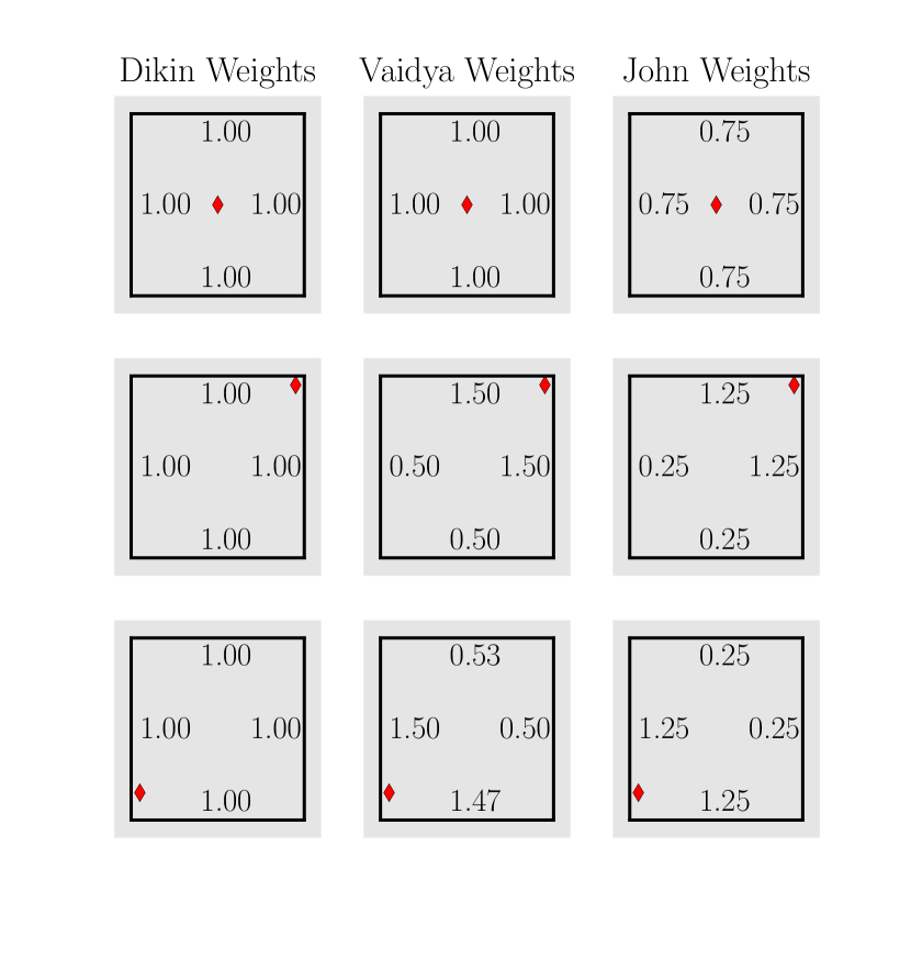
(a) Weights for different locations and a fixed number of constraints $n$.

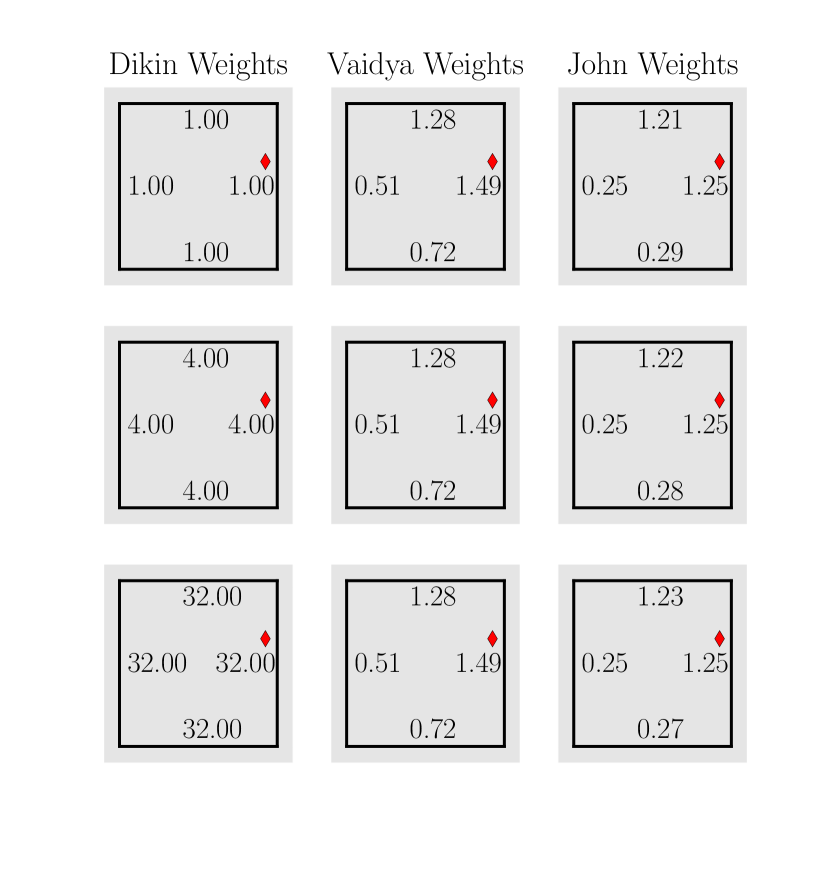
(b) Effective weights for a fixed location and different number of constraints $n$

Figure 1: Visualization of the weights on the square with repeated constraints $\mathcal{S}_{n/4}$ for the different random walks. The number mentioned next to the boundary lines denotes the effective weight for the location $x$ (denoted by diamond) for the corresponding constraint. (a) $n=4$ is common across rows and $x=(0,0)$ for the top row, $(0.9,0.9)$ for the middle and $(-0.9,-0.7)$ for the bottom row. The Dikin weights are independent of $x$, the Vaidya and the John weights for a constraint increase if the location $x$ is closer to it. (b) $x=(0.85,0.30)$ is common across rows, and $n\!=\!4$ for the top row, $n=16$ for the middle and $n\!=\!128$ for the bottom row. The effective Dikin weight for each constraint increases linearly with $n$ but for the Vaidya and John walk adaptively, the weights get adjusted such that the sum of their weights is always of the order of the dimension $d$.

In Figure 1(b)-2(b), we demonstrate that the Vaidya walk and the John walk are better at handling repeated constraints. Note that we can define the square $[-1,1]^{2}$ as

$$[-1,1]^{2}=\left\{x\in\mathbb{R}^{2}\Bigg{|}Ax\leq b,A=\begin{bmatrix}1&0\\ 0&1\\ -1&0\\ 0&-1\end{bmatrix},b=\begin{bmatrix}1\\ 1\end{bmatrix}\right\}.$$ (13)

Simply repeating the rows of the matrix $A$ several times changes the mathematical formulatiton of the polytope, but does not change the shape of the polytope. We define the square with constraints repeated $n/4$ times $\mathcal{S}_{n/4}$ as

$$\mathcal{S}_{n/4}=\left\{x\in\mathbb{R}^{2}\Bigg{|}A_{n/4}x\leq b_{n/4},A_{n/4}=\begin{bmatrix}A\\ \vdots\\ \scriptstyle\times\left(n/4\right)\end{bmatrix},b_{n/4}=\begin{bmatrix}b\\ \vdots\\ \scriptstyle\times\left(n/4\right)\end{bmatrix},\right\}$$ (14)

where $A$ and $b$ were defined above. We denote effective weight for each distinct constraint as the sum of weights corresponding to the same constraint. Using this definition, the effective Dikin weight, which is $n/4$, is thus affected by the repeating of constraints. Consequently, the Dikin ellipsoid is much smaller for polytopes with repeated constraints. However, the Vaidya and John weights do not change as observed in the Figure 1(b). Such a property of these two weights implies that the Vaidya and John ellipsoids are not too small even for very large number of constraints. And we observe such a phenomenon in Figures 2(a)-2(b) where the repetition of rows in the matrix $A$ leads to very small Dikin ellipsoid but large Vaidya and John ellipsoid. A few other numerical computations also suggest that the Vaidya and John ellipsoids are moder adaptive when compared to Dikin ellipsoids when the number of constraints is large. Nonetheless, such a claim is only based on heuristics and is presented simply to provide an intuition that the new ellipsoids are better behaved than Dikin ellipsoids and thereby motivated the design of the new random walks.

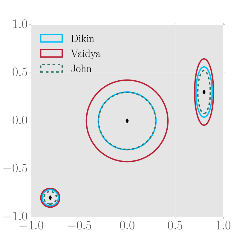
(a) $n=32$

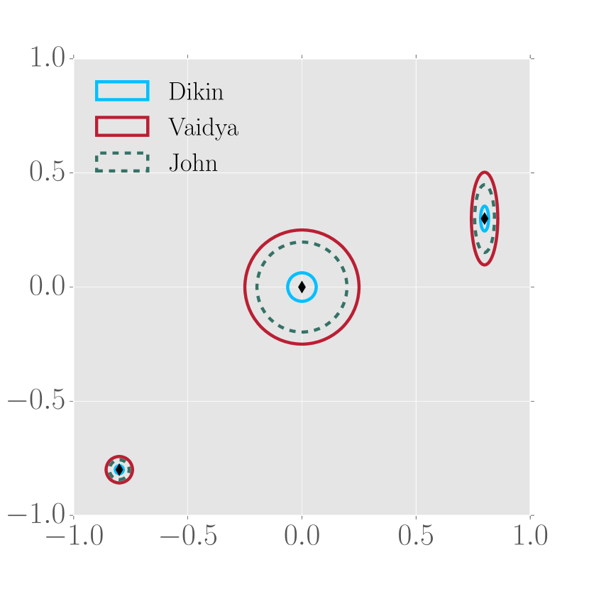
(b) $n=2048$

Figure 2: Visualization of the proposal distribution on the square with repeated constraints $\mathcal{S}_{n/4}$ for the different random walks. (a, b) Unit ellipsoids associated with the covariances of the random walks at different states $x$ on the square with repeated constraints $\mathcal{S}_{n/4}$. Clearly, all these ellipsoids adapt to the boundary but increasing $n$ has a profound impact on the volume of the Dikin ellipsoids and comparatively less impact on the Vaidya and John ellipsoids.

3 Main results

With the basic background in place, we now describe the algorithms more precisely and state upper bounds on the mixing time of the Vaidya and John walks. In Section 3.4, we propose a variant of the John walk, known as the improved John walk, and conjecture that it has a better mixing time bound than that of the John walk.

3.1 Vaidya and John walks

In this subsection, we formally define the Vaidya and John walks. In Algorithm 1 and Algorithm 2, we summarize the steps of the Vaidya walk and the John walk.

Vaidya walk:

The Vaidya walk with radius parameter $r>0$, denoted by VW($r$) for short, is defined by a Gaussian proposal distribution denoted as $\mathcal{P}_{x}^{\text{\tiny V}}$: given a current state $x\in\operatorname{int}\left(\mathcal{K}\right)$, it proposes a new point by sampling from the multivariate Gaussian distribution $\mathcal{N}\left(x,\frac{r^{2}}{\sqrt{nd}}{V_{x}}^{-1}\right)$. In analytic terms, the proposal density at $x$ is given by

$$p^{\text{\tiny V}}_{x}(z):=p_{\text{\tiny Vaidya}(r)}(x,z)=\sqrt{\det{V_{x}}}\left(\frac{nd}{2\pi r^{2}}\right)^{d/2}\exp\left(-\frac{\sqrt{nd}}{2r^{2}}\ (z-x)^{\top}V_{x}(z-x)\right).$$ (15)

As the target distribution for our walk is the uniform distribution on $\mathcal{K}$, the proposal step is followed by an accept-reject step as described in Section 2.1 (equation 1). Thus the overall transition distribution for the walk at state $x$ is defined by a density given by

$$q_{\text{\tiny Vaidya}(r)}(x,z)=\begin{cases}\min\left\{p^{\text{\tiny V}}_{x}(z),p^{\text{\tiny V}}_{z}(x)\right\},&z\in\mathcal{K}\text{ and }z\neq x,\\ 0,&z\notin\mathcal{K},\end{cases}$$

and a probability mass at $x$, given by $1-\int\displaylimits_{z\in\mathcal{K}}\min\left\{p_{x}(z),p_{z}(x)\right\}dz$. We use ${\mathcal{T}}_{\text{\tiny Vaidya}(r)}$ to denote the resulting transition operator for the Vaidya walk with parameter $r$.

Input: Parameter $r$ and $x_{0}\in\operatorname{int}\left(\mathcal{K}\right)$

Output: Sequence $x_{1},x_{2},\ldots$

1 for $i=0,1,\ldots$ do

2       With probability $\frac{1}{2}$ stay at the current state: $x_{i+1}\leftarrow x_{i}$  % lazy step

3       With probability $\frac{1}{2}$ perform the following update:

4        Proposal step: Draw $z_{i+1}\sim\mathcal{N}\left(x_{i},\frac{r^{2}}{(nd)^{1/2}}V_{x_{i}}^{-1}\right)$

5        Accept-reject step:

6         if $z_{i+1}\notin\mathcal{K}$ then $x_{i+1}\leftarrow x_{i}$  % reject an infeasible proposal

7         else

8          compute $\alpha_{i+1}=\displaystyle\min\left\{1,{p_{z_{i+1}}(x_{i+1})}/{p_{x_{i+1}}(z_{i+1})}\right\}$

9          With probability $\alpha_{i+1}$ accept the proposal: $x_{i+1}\leftarrow z_{i+1}$

10          With probability $1-\alpha_{i+1}$ reject the proposal: $x_{i+1}\leftarrow x_{i}$

11 end for

Algorithm 1 Vaidya Walk with parameter $r$ (VW($r$))

John walk:

The John walk is similar to the Vaidya walk except that the proposals at state $x\in\operatorname{int}\left(\mathcal{K}\right)$ are generated from the multivariate Gaussian distribution $\mathcal{N}\left(x,\frac{r^{2}}{d^{3/2}\cdot\log_{2}^{4}(2n/d)}{J_{x}}^{-1}\right)$, where the matrix $J_{x}$ is defined by equation (11), and $r>0$ is a constant. The proposal distribution at $x\in\operatorname{int}\left(\mathcal{K}\right)$ is denoted as $\mathcal{P}_{x}^{\text{\tiny J}}$. The proposal step is then followed by an accept-reject step similarly defined as in the Vaidya walk. We use ${\mathcal{T}}_{\text{\tiny John}(r)}$ to denote the resulting transition operator for the John walk with parameter $r$.

Input: Parameter $r$ and $x_{0}\in\operatorname{int}\left(\mathcal{K}\right)$

Output: Sequence $x_{1},x_{2},\ldots$

1 for $i=0,1,\ldots$ do

2       With probability $\frac{1}{2}$ stay at the current state: $x_{i+1}\leftarrow x_{i}$  % lazy step

3       With probability $\frac{1}{2}$ perform the following update:

4        Proposal step: Draw $z_{i+1}\sim\mathcal{N}\left(x_{i},\frac{r^{2}}{d^{3/2}}J_{x_{i}}^{-1}\right)$  % this step is different than the Vaidya walk

5        Accept-reject step:

6         if $z_{i+1}\notin\mathcal{K}$ then $x_{i+1}\leftarrow x_{i}$  % reject an infeasible proposal

7         else

8          compute $\alpha_{i+1}=\displaystyle\min\left\{1,{p_{z_{i+1}}(x_{i+1})}/{p_{x_{i+1}}(z_{i+1})}\right\}$

9          With probability $\alpha_{i+1}$ accept the proposal: $x_{i+1}\leftarrow z_{i+1}$

10          With probability $1-\alpha_{i+1}$ reject the proposal: $x_{i+1}\leftarrow x_{i}$

11 end for

Algorithm 2 John Walk with parameter $r$ (JW($r$))

3.2 Mixing time bounds for warm start

We are now ready to state an upper bound on the mixing time of the Vaidya walk. In this and other theorem statements, we use $c$ to denote a universal positive constant. Recall that $\pi^{*}$ denotes the uniform distribution on the polytope $\mathcal{K}$, and, that ${\mathcal{T}}_{\text{\tiny Vaidya}(r)}$ denotes the operator on distributions associated with the Vaidya walk.

Theorem 1

Let $\mu_{0}$ be any distribution that is $M$-warm with respect to $\pi^{*}$ as defined in equation (Warm-Start). For any $\delta\in(0,1]$, the Vaidya walk with parameter $r_{\text{\tiny V}}=10^{-4}$ satisfies

$$\|{\mathcal{T}}_{\text{\tiny Vaidya}(r_{\text{\tiny V}})}^{k}(\mu_{0})-\pi^{*}\|_{\mbox{\tiny{TV}}}\leq\delta\qquad\mbox{for all }\;k\geq cn^{{1}/{2}}d^{{3}/{2}}\,\log\left(\frac{\sqrt{M}}{\delta}\right).$$ (16)

The proof of Theorem 1 is provided in Section 5. Theorem 1 precisely quantifies the dependence of mixing time of the Vaidya walk on many parameters of interest such as dimension $d$, number of constraints $n$, the error tolerance $\delta$ and the warmness $M$. The specific choice $r_{\text{\tiny V}}=10^{-4}$ is for theoretical purposes; in practice, we find that substantially larger values can be used. Our upper bound for the mixing time of the Vaidya walk has $\mathcal{O}({{\sqrt{n/d}}})$ improvement over the current best upper bound for the mixing time of the Dikin walk. In Section 4.1, we show that the per iteration cost for the two walks is of the same order. Since $n\geq d$ for closed polytopes in ^d, the effective cost until convergence (iteration complexity multiplied by number of iterations required) for the Vaidya walk is at least of the same order as of the Dikin walk, and significantly smaller when $n\gg d$. Comparing the provable mixing time upper bounds, the Vaidya walk has an advantage over the Dikin walk for the problems where the number of constraints is significantly larger than the number of variables involved. Our simulations also confirm this theoretical finding.

Let us now state our result for the mixing time of the John walk:

Theorem 2

Suppose that $n\leq\exp(\sqrt{d})$, and let $\mu_{0}$ be any distribution that is $M$-warm with respect to $\pi^{*}$. Then for any $\delta\in(0,1]$, the John walk with parameter $r_{\text{\tiny J}}=10^{-5}$ satisfies

$$\|{\mathcal{T}}_{\text{\tiny John}(r_{\text{\tiny J}})}^{k}(\mu_{0})-\pi^{*}\|_{\mbox{\tiny{TV}}}\leq\delta\qquad\text{ for all }k\geq c\;d^{2.5}\,\log^{4}\left(\frac{n}{d}\right)\,\log\left(\frac{\sqrt{M}}{\delta}\right).$$

The proof of Theorem 2 is provided in Appendix D. Again the specific choice of $r_{\text{\tiny J}}=10^{-5}$ is for theoretical purpose; in practice larger choices are possible. Note that the mixing time bound for the John walk depends only on the number of constraints $n$ via a logarithmic factor, and so is almost independent of $n$. Consequently, it has a mixing time that is polynomial in $d$ even if the number of constraints $n$ scales exponentially in $\sqrt{d}$. Further, we show in Section 4.1 that the cost to execute one step of the John walk is of the same order as of the Dikin walk up to a poly-logarithmic factor in $n$. Thus, using John walk, we obtain improved mixing time bounds for the case when $n\gg d^{2}$.

3.3 Mixing time bounds from deterministic start

The mixing time bounds in Theorem 1 and 2 depend on the warmness $M$ of the initial distribution. In some applications, it may not be easy to find an $M$-warm initial distribution. In such cases, we can consider starting the random walk from a deterministic point $x_{0}\in\operatorname{int}\left(\mathcal{K}\right)$ that is not too close to the boundary $\partial\mathcal{K}$. Indeed, such a point can be found using standard optimization methods—e.g., using a Phase-I method for Newton’s algorithm (see Boyd and Vandenberghe, 2004, Section 11.5.4).

Given such a deterministic initialization, our mixing time guarantees depend on the distance of the starting point from the boundary. This dependence involves the following notion of $s$-centrality:

Definition 3

A point $x\in\operatorname{int}\left(\mathcal{K}\right)$ is called $s$-central if for any chord $\overline{ef}$ with end points $e,f\in\partial\mathcal{K}$ passing through $x$, we have $\left\|e-x\right\|_{2}/\left\|f-x\right\|_{2}\leq s$.

Assuming that it is started at an $s$-central point $x_{0}$, the Dikin walk (Kannan and Narayanan, 2012, algorithm in section 2.1) has a polynomial mixing time. The authors showed that when the walk moves to a new state for the first time, the distribution of the iterate is $\mathcal{O}\left((\sqrt{n}s)^{d}\right)$-warm with respect to the distribution $\pi^{*}$. Since only constant number of steps is required to get a warm start, for a deterministic start, we can just use the Dikin walk in the beginning to provide a warm start to the Vaidya (or John) walk. This motivates us to define the following hybrid walk.

Given an $s$-central point $x_{0}$, simulate the Dikin walk until we observe a new state. Note that due to laziness and the accept-reject step, the chain can stay at the starting point for several steps before making the first move a new state. Let $k_{1}$ denote the (random) number of steps taken to make the first move to a new state. After $k_{1}$ steps, we run the walk VW($r$) with $x_{k_{1}}$ as the initial point. We call such a walk as $s$-central Dikin-start-Vaidya-walk with parameter $r$. Let $\mathcal{T}_{\text{Dikin}}$ denote the transition kernel of the Dikin walk stated above. Then, we have the following mixing time bound for this hybrid walk.

Corollary 4

Any $s$-central Dikin-start-Vaidya-walk with parameter $r=10^{-4}$ satisfies

$$\|{\mathcal{T}}_{\text{\tiny Vaidya}(r)}^{k}\big{(}{\mathcal{T}}_{\text{\tiny Dikin}}^{k_{1}}(\delta_{x_{0}})\big{)}-\pi^{*}\|_{\mbox{\tiny{TV}}}\leq\delta\qquad\text{ for all }k\geq cn^{{1}/{2}}d^{{5}/{2}}\,\log\left(\frac{ns}{\delta}\right),$$

where $k_{1}$ is a geometric random variable with ${\mathbb{E}}\left[k_{1}\right]\leq c^{\prime}$, and $c,c^{\prime}>0$ are universal constants.

The mixing rate is logarithmic in $ns$ and has an extra factor of $d$ compared to the bounds in Theorem 1. However, guaranteeing a warm start for a general polytope is hard but obtaining a central point involves only a few steps of optimization. Consequently, the hybrid walk and the guarantees from Corollary 4 come in handy for all such cases. Once again we observe that the upper bounds for mixing time are improved by a factor of $\mathcal{O}({\sqrt{n/d}})$ when compared to the Dikin walk from an $s$-central start (Kannan and Narayanan, 2012; Narayanan, 2016) which had a mixing time of $\mathcal{O}\left(nd^{2}\right)$. The proof follows immediately from Theorem 1 by Kannan and Narayanan (2012) and Theorem 1 of this paper and is thereby omitted.

In a similar fashion, we can provide a polynomial time guarantee for a modified John walk from a deterministic start. We can consider a hybrid random walk that starts at an $s$-central point, simulates the Dikin walk until it makes the first move to a new state, and from there onwards simulates the John walk. Such a chain would have a mixing time of $\mathcal{O}\left(d^{3.5}\text{poly-log}(n,d,s)\right)$. For brevity, we omit a formal statement of this result.

3.4 Conjecture on improved John walk

From our analysis, we suspect that it is possible to improve the mixing time bound of $\mathcal{O}\left(d^{2.5}\text{poly-log}(n/d)\right)$ in Theorem 2 by considering a variant of the John walk. In particular, we conjecture that a random walk with proposal distribution given by $\mathcal{N}\left(x,\frac{r^{2}}{d\cdot\text{poly-log}(n/d)}{J_{x}}^{-1}\right)$ for a suitable choice of $r$ has an $\mathcal{O}\left(d^{2}\text{poly-log}(n/d)\right)$ mixing time from a warm start. We refer to this random walk as the improved John walk, and denote its transition operator by $\mathcal{T}_{\text{\tiny John${}^{+}$}}$. Let us now give a formal statement of our conjecture on its mixing rate.

Conjecture 5

Let $\mu_{0}$ be any $M$-warm distribution. Then for any $\delta\in(0,1]$, the improved John walk with parameter $r=r_{0}$, satisfies the bound

$$\|\mathcal{T}_{\text{\tiny John${}^{+}$}}^{k}(\mu_{0})-\pi^{*}\|_{\mbox{\tiny{TV}}}\leq\delta\qquad\mbox{ for all }k\geq c\>d^{2}\,\log_{2}^{c^{\prime}}\left(\frac{2n}{d}\right)\,\log\left(\frac{\sqrt{M}}{\delta}\right),$$

where $r_{0},c,c^{\prime}$ are universal constants.

Note that this conjecture involves quadratic (degree two) scaling in $d$; this exponent of two matches the sum of exponents for $d$ and $n$ in the mixing time bounds for both the Dikin and Vaidya walks from a warm-start. Consquently, the improved John walk would have better performance than the Dikin, Vaidya and John walks for almost all ranges of $(n,d)$, apart from possible poly-logarithmic factors in the ratio $n/d$.

3.5 Proof sketch

In this subsection, we provide a high-level sketch of the main ingredients of the main proof. It is well-known that mixing of a Markov chain is closely related to its conductance. Our main proof relies on the work by Lovász (1999) that characterizes the conductance of Markov chains on a convex set using Hilbert metric. Precisely, Lovász (1999) showed that a Markov chain has good conductance if it makes jumps to regions with large overlaps from two nearby points and the mixing time depends inversely on the maximum Hilbert metric between such nearby points. Using this argument, it remains to make sure that the ellipsoid radius is chosen properly such that the ellipsoids remain inside the polytope and the ellipsoids corresponding to two different points $x$ and $y$ overlap a lot even if the points $x$ and $y$ are relatively far apart.

The conductance-based argument has been used for analyzing the ball walk (Lovász and Simonovits, 1990, 1993), Hit-and-run (Lovász, 1999; Lovász and Vempala, 2006a) and the Dikin walk (Kannan and Narayanan, 2012; Narayanan, 2016; Sachdeva and Vishnoi, 2016). We refer the reader to the survey by Vempala (2005) for a thorough discussion about the relation between the conductance and mixing time for Markov chains. Our proof techniques share a few features with the recent analyses of the Dikin walk by Kannan and Narayanan (2012) and Sachdeva and Vishnoi (2016). However, new technical ideas are needed in order to handle the state-dependent weights $\sigma_{x}$ and $\zeta_{x}$, as defined in equations (9b) and (12) respectively, that underlie the proposal distributions for the Vaidya and John walks. Note that these techniques are not present in the analysis of the Dikin walk, which is based on constant weights.

Specifically, we present the proof of Theorem 1 on the mixing time of the Vaidya walk in Section 5 and defer the intermediate technical results to Appendix A, B and C. We present the proof of Theorem 2 (mixing time bound for the John walk) in Appendix D and provide related auxiliary results and their proofs in Appendices E, F, G, H and I. As alluded to earlier, to keep the paper self-contained, we provide the proof of Lovász’s Lemma in Appendix J.

4 Numerical experiments

In this section, we first analyze the per-iteration cost to implement of three walks. We show that while the Dikin walk has the best per-iteration cost, the per-iteration cost of the Vaidya walk is only twice of that of Dikin walk and the per-iteration cost of the John walk is only of order $\log_{2}(2n/d)$ larger. Second, we demonstrate the speed-up gained by the Vaidya walk over the Dikin walk for a warm start on different polytopes.

4.1 Per iteration cost

We now show that the per iteration cost of the Dikin, Vaidya and John walks is of the same order. The proposal step of Vaidya walk requires matrix operations like matrix inversion, matrix multiplication and singular value decomposition (SVD). The accept-reject step requires computation of matrix determinants, besides a few matrix inverses and matrix-vector products. The complexity of all aforementioned operations is $\mathcal{O}\left(nd^{2}\right)$. Thus, per iteration computational complexity for the Vaidya walk is $\mathcal{O}\left(nd^{2}\right)$.

Both the Dikin and Vaidya walks requires an SVD computation for inverting the Hessian of Dikin barrier $\nabla^{2}\mathcal{F}_{x}$. In addition for the Vaidya walk, we have to invert the matrix $V_{x}$, which leads to almost twice the computation time of the Dikin walk per step. This difference can be observed in practice.

For the John walk, we need to compute the weights $\zeta_{x}$ at each point which involves solving the program (12). Lee and Sidford (2014) argued that the convex program (12) for obtaining John walk’s weights is strongly convex with a suitably chosen norm. They proved that solving this program requires $\log^{2}n$ number of gradient steps, where the computational complexity of each gradient step is equivalent to that of solving an $n\times d$ linear system ($\mathcal{O}\left(nd^{2}\right)$ using a numerically stable routine). Thus, the overall cost for the John walk is of the same order as of the Dikin walk up to a poly-logarithmic factor in the pair $(n,d)$.

In practice, for the John walk, the combined effect of logarithmic factors in the number of steps and the cost to implement each step cannot be ignored. This extra factor becomes a bottleneck for the overall run time for the convergence of the Markov chain. Consequently, the John walk is not suitable for polytopes with moderate values of $n$ and $d$, and its mixing time bounds are computationally superior to the Dikin and Vaidya walks only for the polytopes with $n\gg d\gg 1$.

4.2 Simulations

We now present simulation results for the random walks in ^d for $d=2,10$ and $50$ with initial distribution $\mu_{0}=\mathcal{N}(0,\sigma_{d}^{2}\,\mathbb{I}_{d})$ and target distribution being uniform, on the following polytopes:

1. : The set $[-1,1]^{2}$ defined by different number of constraints.

2. : The set $[-1,1]^{d}$ for $d\in\{2,3,4,5,6,7\}$ for $n=\{2d,2d^{2},2d^{3}\}$ constraints.

3. : Symmetric polytopes in ² with $n$-randomly-generated-constraints.

4. : The interior of regular $n$-polygons on the unit circle.

5. : Hyper cube $[-1,1]^{d}$ for $d=10$ and $50$.

We choose $\sigma_{d}$ such that the warmness parameter $M$ is bounded by $100$. We provide implementations of the Dikin, Vaidya and John walks in python and a jupyter notebook at the github repository https://github.com/rzrsk/vaidya-walk.

We use the following three ways to compare the convergence rate of the Dikin and the Vaidya walks: (1) comparing the approximate mixing time of a particular subset of the polytope—smaller value is associated with a faster mixing chain; (2) comparing the plot of the empirical distribution of samples from multiple runs of the Markov chain after $k$ steps—if it appears more uniform for smaller $k$, the chain is deemed to be faster; and (3) contrasting the sequential plots of one dimensional projection of samples for a single long run of the chain—less smooth plot is associated with effective and fast exploration leading to a faster mixing (Yu and Mykland, 1998). Note that MCMC convergence diagnostics is a hard problem, especially in high dimensions, and since the methods outlined above are heuristic in nature we expect our experiments to not fully match our theoretical results.

In Set-up 1, we consider the polytope $[-1,1]^{2}$ which can be represented by exactly $4$ linear constraints (see Section 2.4). Suppose that we repeat the rows of the matrix $A$, and then run the Dikin and Vaidya walks with the new $A$. Given the larger number of constraints, our theory predicts that the random walks should mix more slowly. In Figure 3(c) and 3(d), we plot the empirical distribution obtained by the Dikin walk and Vaidya walk, starting from $200$ i.i.d initial samples, for $n=64$ and $2048$. The empirical distribution plot shows that having large $n$ significantly slows the mixing rate of the Dikin walk, while the effect on the Vaidya walk is much less. Further, we also plot the scaling of the approximate mixing time $\hat{k}_{\text{mix}}$ (defined below) for this simulation as a function of the number of constraints $n$ in Figure 3(b). For Set-up 2, we plot $\hat{k}_{\text{mix}}$ as a function of the dimensions $d$ in Figures 3(e)-3(g), for the random walks on $[-1,1]^{d}$ where the hypercube is parametrized by different number of constraints $n\in\{2d,2d^{2},2d^{3}\}$. The approximate mixing time is defined with respect to the set $\mathcal{S}_{d}=\{x\in{}^{d}|\left|x_{i}\right|\geq c_{d}\ \forall i\in[d]\}$ where $c_{d}$ is chosen such that $\pi^{*}(\mathcal{S}_{d})=1/2$. In particular, for a fixed value of $n$, let $\hat{\mathbb{T}}^{k}$ denote the empirical measure after $k$-iterations across $2000$ experiments. The approximate mixing time $\hat{k}_{\text{mix}}$ is defined as

$$\hat{k}_{\text{mix}}:=\min\left\{k\bigg{|}{\pi^{*}(\mathcal{S}_{d})-\hat{\mathbb{T}}^{k}(\mathcal{S}_{d})}\leq\frac{1}{20}\right\},$$ (17)

We choose such a set since the set covers the regions near to the boundary of the polytope which are not covered well by the chosen initial distribution. We make the following observations:

1. The slopes of the best-fit lines, for $\hat{k}_{\text{mix}}$ versus $n$ in the log-log plot in Figure 3(b), are $0.88$ and $0.45$ for Dikin and Vaidya walks respectively. This observation reflects a near-linear and sub-linear dependence on $n$ for a fixed $d$ for the mixing time of the Dikin walk and the Vaidya walk respectively.

2. In Figures 3(e)-3(g), once again we observe a more significant effect of increasing the number of constraints on the approximate mixing time $\hat{k}_{\text{mix}}$. We list the slopes of the best fit lines on these log-log plots in Table 2. These slopes correspond to the exponents for $d$ for the approximate mixing time. From the table, we can observe that these experiments agree with the mixing time bounds of $\mathcal{O}\left(nd\right)$ for the Dikin walk and $\mathcal{O}\left(n^{0.5}d^{1.5}\right)$ for the Vaidya walk.

No. of Constraints	DW Theoretical	VW Theoretical	DW Experiments	VW Experiments
$n=2d$	$2.0$	$2.0$	$1.58$	$1.72$
$n=2d^{2}$	$3.0$	$2.5$	$2.80$	$2.48$
$n=2d^{3}$	$4.0$	$3.0$	$3.84$	$2.75$

Table 2: Value of the exponent of dimensions $d$ for the theoretical bounds on mixing time and the observed approximate mixing time of the Dikin walk (DW) and the Vaidya walk (VW) for $[-1,1]^{d}$ described by $n=2d,2d^{2},2d^{3}$ constraints. The theoretical exponents are based on the mixing time bounds of $\mathcal{O}\left(nd\right)$ for the Dikin walk and $\mathcal{O}\left(n^{0.5}d^{1.5}\right)$ for the Vaidya walk. The experimental exponents are based on the results from the simulations described in Set-up 2 in Section 4.2. Clearly, the exponents observed in practice are in agreement with the theoretical rates and imply the faster convergence of the Vaidya walk compared to the Dikin walk for large number of constraints.

In Set-up 3, we compare the plots of the empirical distribution of $200$ runs of the Dikin walk and the Vaidya walk for different values of $k$, for symmetric polytopes in ² with $n$-randomly-generated-constraints. We fix $b_{i}=1$. To generate $a_{i}$, first we draw two uniform random variables from $[0,1]$ and then flip the sign of both of them with probability $1/2$ and assign these values to the vector $a_{i}$. The resulting polytope is always a subset of the square $\mathcal{K}=[-1,1]^{2}$ and contains the diagonal line connecting the points $(-1,1)$ and $(1,-1)$. From Figure 4(a)-4(b), we observe that while there is no clear winner for the case $n=64$, the Vaidya walk mixes mixes significantly faster than the Dikin walk for the polytope defined by $2048$ constraints.

In Set-up 4, the constraint set is the regular $n$-polygons inscribed in the unit circle. A similar observation as in Set-up 3 can be made from Figure 4(c)-4(d): the Vaidya walk mixes at least as fast as the Dikin walk and mixes significantly faster for large $n$.

In Set-up 5, we examine the performance of the Dikin walk and the Vaidya walk on hyper-cube $[-1,1]^{d}$ for $d=10,50$. We plot the one dimensional projections onto a random normal direction of all the samples from a single run up to $10,000$ steps. The Vaidya sequential plot looks more jagged than that of the Dikin walk for $d=10,n=5120$. For other cases, we do not have a clear winner. Such an observation is consistent with the $\mathcal{O}({\sqrt{n/d}})$ speed up of the Vaidya walk which is apparent when the ratio $n/d$ is large.

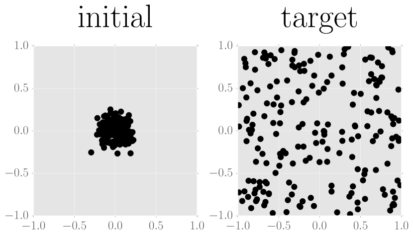
(a)

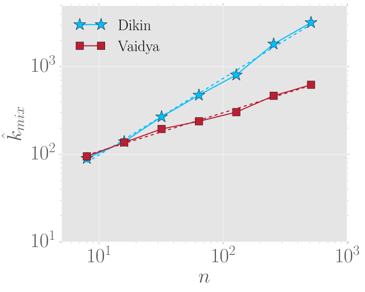
(b)

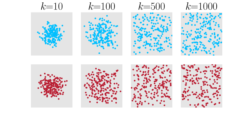
(c) $n=64$

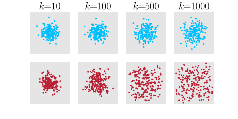
(d) $n=2048$

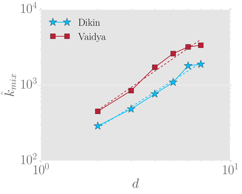
(e) $n=2d$

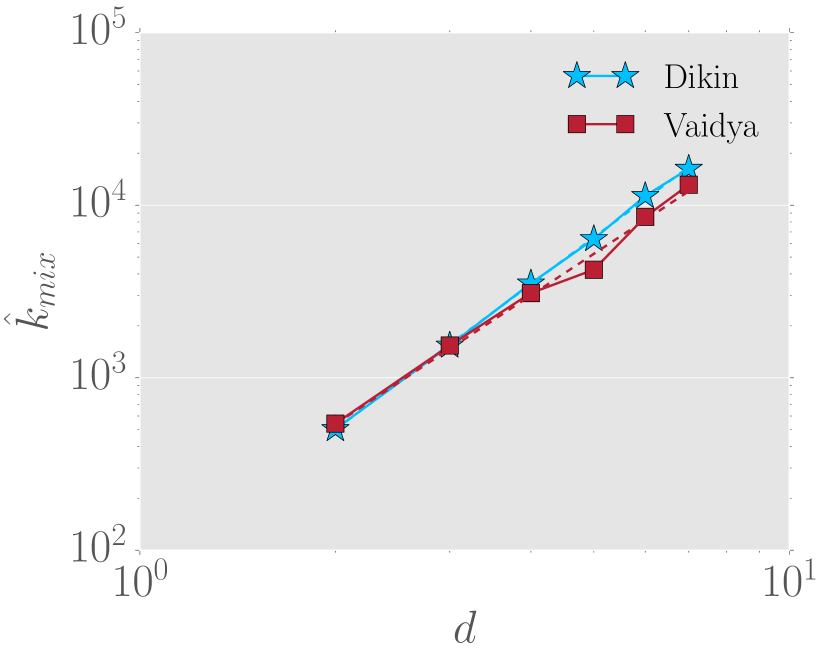
(f) $n=2d^{2}$

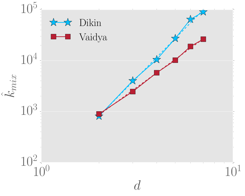
(g) $n=2d^{3}$

Figure 3: Comparison of the Dikin and Vaidya walks on the polytope $\mathcal{K}=[-1,1]^{2}$. (a) Samples from the initial distribution $\mu_{0}=\mathcal{N}(0,0.04\,\mathbb{I}_{2})$ and the uniform distribution on $[-1,1]^{2}$. (b) Log-log plot of $\hat{k}_{\text{mix}}$ (17) versus the number of constraints ($n$) for a fixed dimension $d=2$. (c, d) Empirical distribution of the samples for the Dikin walk (blue/top rows) and the Vaidya walk (red/bottom rows) for different values of $n$ at iteration $k=10,100,500$ and $1000$. (e, f, g) Log-log plot of $\hat{k}_{\text{mix}}$ vs the dimension $d$, for $n\in\{2d,2d^{2},2d^{3}\}$ for $d\in\{2,3,4,5,6,7\}$. The exponents from these plots are summarized in Table 2. Note that increasing the number of constraints $n$ has more profound effect on the Dikin walk in almost all the cases.

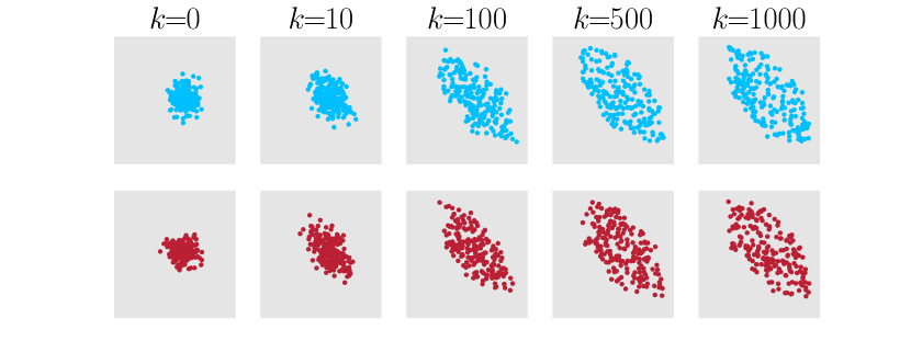
(a) $n=64$

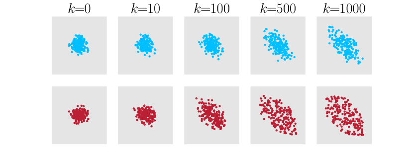
(b) $n=2048$

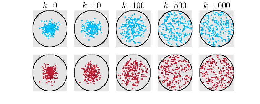
(c) $n=64$

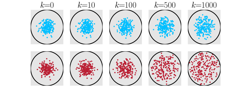
(d) $n=2048$

Figure 4: Empirical distribution of the samples from $200$ runs for the Dikin walk (blue/top rows) and the Vaidya walk (red/bottom rows) at different iterations $k$. The $2$-dimensional polytopes considered are: (a, b) random polytopes with $n$-constraints, and (c, d) regular $n$-polygons inscribed in the unit circle. For both sets of cases, we observe that higher $n$ slows down the walks, with visibly more effect on the Dikin walk compared to the Vaidya walk.

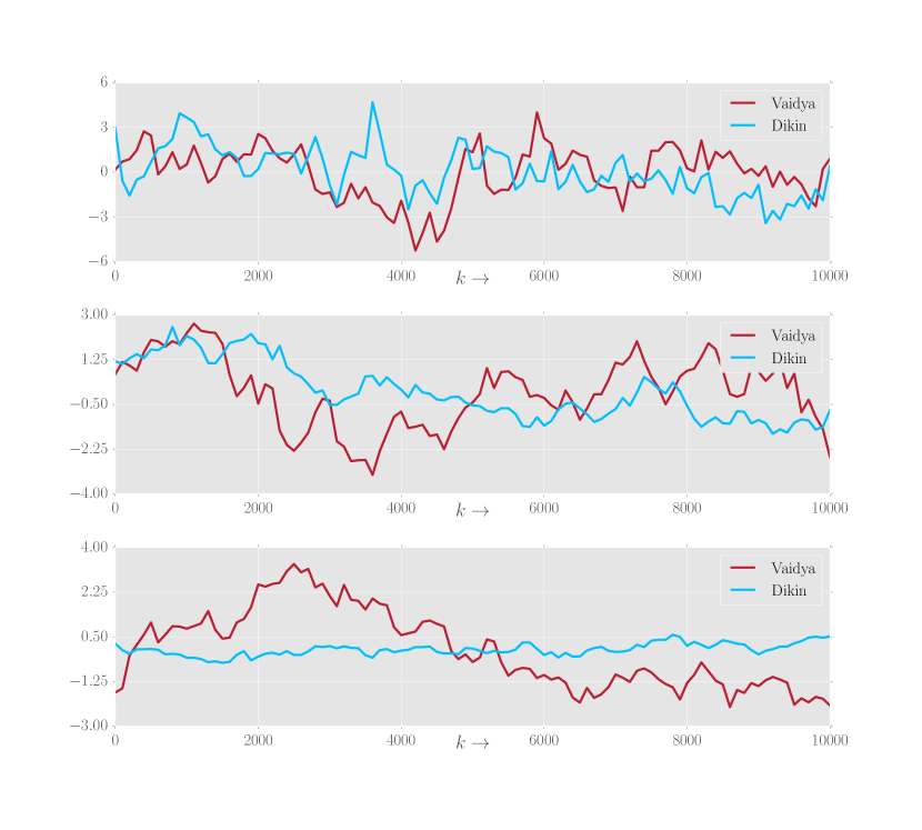
(a) $d=10$

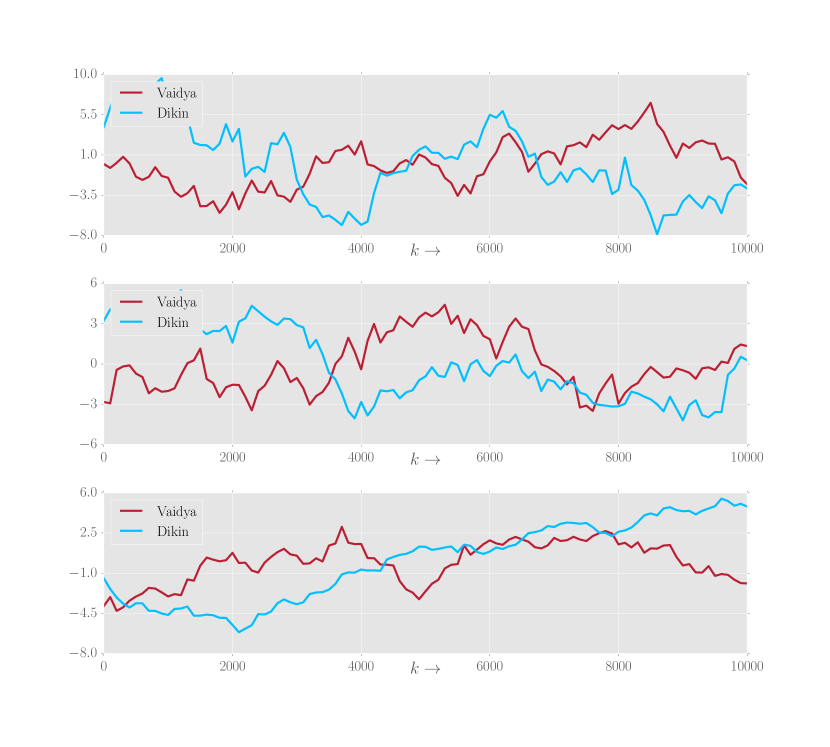
(b) $d=50$

Figure 5: Sequential plots of a one-dimensional random projection of the samples on the hyperbox $\mathcal{K}=[-1,1]^{d}$, defined by $n$ constraints. Each plot corresponds to one long run of the Dikin and Vaidya walks, and the projection is taken in a direction chosen randomly from the sphere. (a) Plots for $d=10$ and $n\in\{20,640,5120\}$. (b) Plots for $d=50$ and $n\in\{100,400,1600\}$. Relative to the Dikin walk, the Vaidya walk has a more jagged plot for pairs $(n,d)$ in which the ratio $n/d$ is relatively large: for instance, see the plots corresponding to $(n,d)=(640,10)$ and $(5120,10)$. The same claim cannot be made for pairs $(n,d)$ for which the ratio $n/d$ is relatively small; e.g., the plot with $(n,d)=(20,10)$. These observations are consistent with our results that the Vaidya walk mixes more quickly by a factor of order $\mathcal{O}({{\sqrt{n/d}}})$ over the Dikin walk.

5 Proofs

We begin with auxiliary results in Section 5.1 which we use then to prove Theorem 1 in Section 5.2. Proofs of the auxiliary results are in Sections 5.3 and 5.4, and we defer other technical results to appendices.

5.1 Auxiliary results

Our proof proceeds by formally establishing the following property for the Vaidya walk: if two points are close, then their one-step transition distribution are also close. Consequently, we need to quantify the closeness between two points and the associated transition distributions. We measure the distance between two points in terms of the cross ratio that we define next. For a given pair of points $x,y\in\mathcal{K}$, let $e(x),e(y)\in\partial\mathcal{K}$ denote the intersection of the chord joining $x$ and $y$ with $\mathcal{K}$ such that $e(x),x,y,e(y)$ are in order (see Figure 6(a)). The cross-ratio $d_{\mathcal{K}}(x,y)$ is given by

$$d_{\mathcal{K}}(x,y) :=\frac{\left\|e(x)-e(y)\right\|_{2}\left\|x-y\right\|_{2}}{\left\|e(x)-x\right\|_{2}\left\|e(y)-y\right\|_{2}}.$$ (18)

The ratio $d_{\mathcal{K}}(x,y)$ is related to the Hilbert metric on $\mathcal{K}$, which is given by $\log\left(1+d_{\mathcal{K}}(x,y)\right)$; see the paper by Bushell (1973) for more details.

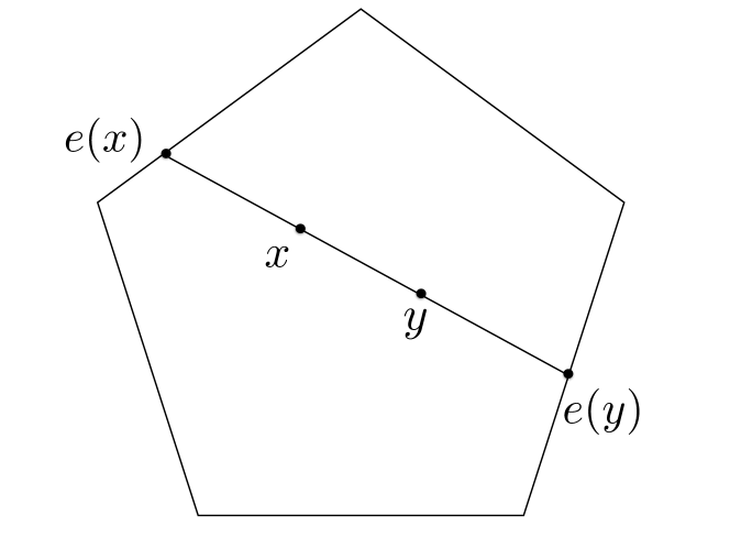
(a)

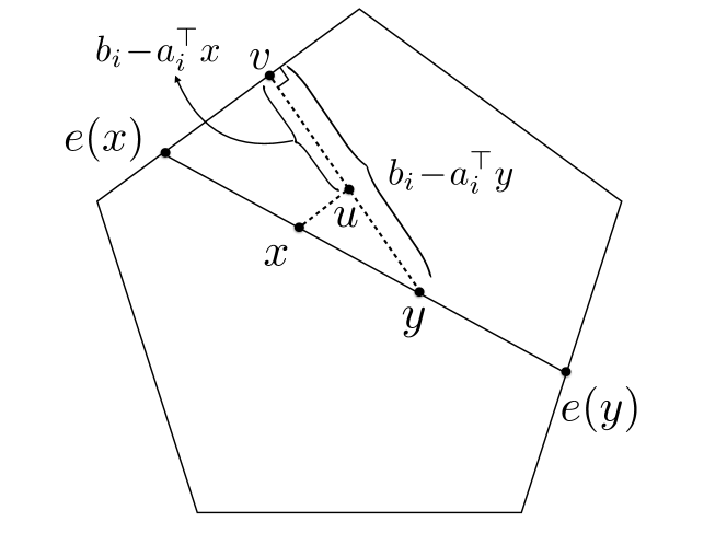
(b)

Figure 6: Polytope $\mathcal{K}=\{x\in{}^{d}|Ax\leq b\}$. (a) The points $e(x)$ and $e(y)$ denote the intersection points of the chord joining $x$ and $y$ with $\mathcal{K}$ such that $e(x),x,y,e(y)$ are in order. (b) A geometric illustration of the argument (23). It is straightforward to observe that ${\left\|x-y\right\|_{2}}/{\left\|e(x)-x\right\|_{2}}={\left\|u-y\right\|_{2}}/{\left\|u-v\right\|_{2}}={\left|a_{i}^{\top}(y-x)\right|}/\left(b_{i}-a_{i}^{\top}x\right)$.

Consider a lazy reversible random walk on a bounded convex set $\mathcal{K}$ with transition operator ${\mathcal{T}}$ defined via the mapping $\mu_{0}\mapsto\mu_{0}/2+\tilde{\mathcal{T}}(\mu_{0})/2$ and stationary with respect to the uniform distribution on $\mathcal{K}$ (denoted by $\pi^{*}$). (Recall that $\mathbf{\delta}_{x}$ denote the dirac-delta distribution with unit mass at $x$.) The following lemma gives a bound on the mixing-time of the Markov chain.

Lemma 6 (Lovász’s Lemma)

Suppose that there exist scalars $\rho,\Delta\in(0,1)$ such that

$$\|\tilde{\mathcal{T}}(\mathbf{\delta}_{x})-\tilde{\mathcal{T}}(\mathbf{\delta}_{y})\|_{\mbox{\tiny{TV}}}\leq 1-\rho\qquad\mbox{for all $x,y\in\operatorname{int}\left(\mathcal{K}\right)$ with $d_{\mathcal{K}}(x,y)<\Delta$.}$$ (19a)

Then for every distribution $$\mu_{0} M \pi^{*} {\mathcal{T}}$$ that is -warm with respect to , the lazy transition operator satisfies

$$\|{\mathcal{T}}^{k}(\mu_{0})-\pi^{*}\|_{\mbox{\tiny{TV}}}\leq\displaystyle\sqrt{M}\exp\left(-k\,\frac{\Delta^{2}\rho^{2}}{4096}\right)\quad\forall\ \ k=1,2,\ldots.$$ (19b)

This result is implicit in the paper by Lovász (1999), though not explicitly stated. In order to keep the paper self-contained, we provide a proof of this result in Appendix J.

Our proof of Theorem 1 is based on applying Lovász’s Lemma; the main challenge in our work is to establish that our random walks satisfy the condition (19a) with suitable choices of $\Delta$ and $\rho$. In order to proceed with the proof, we require a few additional notations. Recall that the slackness at $x$ was defined as $s_{x}:=(b_{1}-a_{1}^{\top}x,\ldots,b_{n}-a_{n}^{\top}x)^{\top}$. For all $x\in\operatorname{int}\left(\mathcal{K}\right)$, define the Vaidya local norm of $v$ at $x$ as

$$\left\|v\right\|_{V_{x}} :=\left\|V_{x}^{1/2}v\right\|_{2}=\sqrt{\sum_{i=1}^{n}(\sigma_{x,i}+\beta_{\text{\tiny V}})\frac{(a_{i}^{\top}v)^{2}}{s_{x,i}^{2}}},$$ (20a)

and the Vaidya slack sensitivity at $$x$$ as

$$\theta_{V_{x}}:=\left(\left\|\frac{a_{1}}{s_{x,1}}\right\|_{V_{x}}^{2},\ldots,\left\|\frac{a_{n}}{s_{x,n}}\right\|_{V_{x}}^{2}\right)^{\top}=\left(\frac{a_{1}^{\top}V_{x}^{-1}a_{1}}{s_{x,1}^{2}},\ldots,\frac{a_{n}^{\top}V_{x}^{-1}a_{n}}{s_{x,n}^{2}}\right)^{\top}.$$ (20b)

Similarly, we define the John local norm of $$v x x$$ at and the John slack sensitivity at as

$$\left\|v\right\|_{J_{x}} :=\left\|J_{x}^{1/2}v\right\|_{2}\quad\text{and}\quad\theta_{J_{x}}:=\left(\left\|\frac{a_{1}}{s_{x,1}}\right\|_{J_{x}}^{2},\ldots,\left\|\frac{a_{n}}{s_{x,n}}\right\|_{J_{x}}^{2}\right)^{\top}.$$ (20c)

The following lemma provides useful properties of the leverage scores $\sigma_{x}$ from equation (9b), the weights $\zeta_{x}$ obtained from solving the program (12), and the slack sensitivities $\theta_{V_{x}}$ and $\theta_{J_{x}}$.

Lemma 7

For any $x\in\operatorname{int}\left(\mathcal{K}\right)$, the following properties hold:

1. $\sigma_{x,i}\in[0,1]$ for all $i\in[n]$,

2. $\sum_{i=1}^{n}\sigma_{x,i}=d$,

3. $\theta_{V_{x},i}\in\left[0,\sqrt{n/d}\right]$ for all $i\in[n]$,

4. $\zeta_{x,i}\in[\beta_{\text{\tiny J}},1+\beta_{\text{\tiny J}}]$ for all $i\in[n]$,

5. $\sum_{i=1}^{n}\zeta_{x,i}=3d/2$, and

6. $\theta_{J_{x},i}\in\left[0,4\right]$ for all $i\in[n]$.

We prove this lemma in Section 5.3.

Let $\mathcal{P}_{x}^{\text{\tiny V}}$ to denote the proposal distribution of the random walk VW($r$) at state $x$. Next, we state a lemma that shows that if two points $x,y\in\operatorname{int}\left(\mathcal{K}\right)$ are close in Vaidya local norm at $x$, then for a suitable choice of the parameter $r$, the proposal distributions $\mathcal{P}^{\text{\tiny V}}_{x}$ and $\mathcal{P}^{\text{\tiny V}}_{y}$ are close. In addition, we show that the proposals are accepted with high probability at any point $x\in\operatorname{int}\left(\mathcal{K}\right)$. To establish the latter result, we now define the non-lazy transition operator of the Vaidya walk. Since the Vaidya walk is lazy with probability $1/2$, there exists a valid (non-lazy) transition operator $\tilde{\mathcal{T}}_{\text{\tiny Vaidya}(r)}$ such that for any distribution $\mu_{0}$, we have

$${\mathcal{T}}_{\text{\tiny Vaidya}(r)}(\mu_{0})=\mu_{0}/2+\tilde{\mathcal{T}}_{\text{\tiny Vaidya}(r)}(\mu_{0})/2.$$

We call $\tilde{\mathcal{T}}_{\text{\tiny Vaidya}}$ the non-lazy transition operator for the Vaidya walk. Note that the one-step non-lazy transition distribution $\tilde{\mathcal{T}}_{\text{\tiny Vaidya}(r)}(\mathbf{\delta}_{x})$ denotes the distribution of proposals after the accept-reject step if the chain was not lazy. Thus to establish that proposals are accepted with high probability, it suffices to establish that the transition distribution $\tilde{\mathcal{T}}_{\text{\tiny Vaidya}(r)}(\mathbf{\delta}_{x})$ at any point $x\in\mathcal{K}$ is close to the proposal distribution $\mathcal{P}_{x}^{\text{\tiny V}}$. We now state these two results formally:

Lemma 8

There exists a continuous non-decreasing function $$f:[0,1/4]\rightarrow{}_{+} f(1/15)\geq 10^{-4} \epsilon\in(0,1/15] r r\in[0,f(\epsilon)]$$ with such that for any , the random walk VW() with satisfies

$$\|\mathcal{P}^{\text{\tiny V}}_{x}-\mathcal{P}^{\text{\tiny V}}_{y}\|_{\mbox{\tiny{TV}}} \leq\epsilon\quad\mbox{ $\forall\ x,y\in\operatorname{int}\left(\mathcal{K}\right)$ s.t. $\left\|x-y\right\|_{V_{x}}\leq\displaystyle\frac{\epsilon r}{2(nd)^{1/4}}$ },\quad\text{and}$$ (21a)

$$\|\tilde{\mathcal{T}}_{\text{\tiny Vaidya}(r)}(\mathbf{\delta}_{x})-\mathcal{P}^{\text{\tiny V}}_{x}\|_{\mbox{\tiny{TV}}} \leq 5\epsilon\,\,\,\mbox{$\forall\ x\in\operatorname{int}\left(\mathcal{K}\right)$.}$$ (21b)

See Section 5.4 for the proof of this lemma.

With these lemmas in hand, we are now equipped to prove Theorem 1. To simplify notation, for the rest of this section, we adopt the shorthands $\mathbb{T}_{x}=\tilde{\mathcal{T}}_{\text{\tiny Vaidya}(r)}(\mathbf{\delta}_{x})$, $\mathcal{P}_{x}=\mathcal{P}_{x}^{\text{\tiny V}}$ and $\left\|\cdot\right\|_{V_{x}}=\left\|\cdot\right\|_{x}$.

5.2 Proof of Theorem 1

In order to invoke Lovász’s Lemma for the random walk VW($10^{-4}$), we need to verify the condition (19a) for suitable choices of $\rho$ and $\Delta$. Doing so involves two main steps:

(A):

First, we relate the cross-ratio $d_{\mathcal{K}}(x,y)$ to the local norm (20a) at $x$.

(B):

Second, we use Lemma 8 to show that if $x,y\in\operatorname{int}\left(\mathcal{K}\right)$ are close in local-norm, then the transition distributions $\mathbb{T}_{x}$ and $\mathbb{T}_{y}$ are close in TV-distance.

Step (A):

We claim that for all $x,y\in\operatorname{int}\left(\mathcal{K}\right)$, the cross-ratio can be lower bounded as

$$d_{\mathcal{K}}(x,y)\geq\frac{1}{\sqrt{2d}}\left\|x-y\right\|_{x}.$$ (22)

Note that we have

$$d_{\mathcal{K}}(x,y)=\frac{\left\|e(x)-e(y)\right\|_{2}\left\|x-y\right\|_{2}}{\left\|e(x)-x\right\|_{2}\left\|e(y)-y\right\|_{2}} \stackrel{{\scriptstyle(i)}}{{\geq}}\max\left\{\frac{\left\|x-y\right\|_{2}}{\left\|e(x)-x\right\|_{2}},\frac{\left\|x-y\right\|_{2}}{\left\|e(y)-y\right\|_{2}}\right\}$$

$$\stackrel{{\scriptstyle(ii)}}{{\geq}}\max\left\{\frac{\left\|x-y\right\|_{2}}{\left\|e(x)-x\right\|_{2}},\frac{\left\|x-y\right\|_{2}}{\left\|e(y)-x\right\|_{2}}\right\},$$

where step (i) follows from the inequality $\left\|e(x)-e(y)\right\|_{2}\geq\max\left\{\left\|e(y)-y\right\|_{2},\left\|e(x)-x\right\|_{2}\right\}$; and step (ii) follows from the inequality $\left\|e(x)-x\right\|_{2}\leq{\left\|e(y)-x\right\|_{2}}$. Furthermore, from Figure 6(b), we observe that

$$\max\left\{\frac{\left\|x-y\right\|_{2}}{\left\|e(x)-x\right\|_{2}},\frac{\left\|x-y\right\|_{2}}{\left\|e(y)-x\right\|_{2}}\right\}=\max_{i\in[n]}\left|\frac{a_{i}^{\top}(x-y)}{s_{x,i}}\right|.$$ (23)

This argument of equation (14) has also been used (Sachdeva and Vishnoi, 2016, lemma 9). Note that maximum of a set of non-negative numbers is greater than the mean of the numbers. Combining this fact with properties (a) and (b) from Lemma 7, we find that

$$d_{\mathcal{K}}(x,y)\geq\sqrt{\frac{1}{\sum_{i=1}^{n}\left(\sigma_{x,i}+\beta_{\text{\tiny V}}\right)}\sum_{i=1}^{n}(\sigma_{x,i}+\beta_{\text{\tiny V}})\frac{(a_{i}^{\top}(x-y))^{2}}{s_{x,i}^{2}}}=\frac{\left\|x-y\right\|_{x}}{\sqrt{2d}},$$

thereby proving the claim (22).

Step (B):

By the triangle inequality, we have

$$\|\mathbb{T}_{x}-\mathbb{T}_{y}\|_{\mbox{\tiny{TV}}}\leq\|\mathbb{T}_{x}-\mathcal{P}_{x}\|_{\mbox{\tiny{TV}}}+\|\mathcal{P}_{x}-\mathcal{P}_{y}\|_{\mbox{\tiny{TV}}}+\|\mathcal{P}_{y}-\mathbb{T}_{y}\|_{\mbox{\tiny{TV}}}.$$

Thus, for any $(r,\epsilon)$ such that $\epsilon\in[0,1/15]$ and $r\leq f(\epsilon)$, Lemma 8 implies that

$$\|\mathbb{T}_{x}-\mathbb{T}_{y}\|_{\mbox{\tiny{TV}}} \leq 11\epsilon,\quad\mbox{$\forall x,y\in\operatorname{int}\left(\mathcal{K}\right)$ such that $\left\|x-y\right\|_{x}\leq\displaystyle\frac{r\epsilon}{2(nd)^{1/4}}$}.$$

Consequently, the walk VW($r$) satisfies the assumptions of Lovász’s Lemma with

$$\Delta:=\frac{1}{\sqrt{2d}}\cdot\frac{r\epsilon}{2(nd)^{1/4}}\quad\mbox{and}\quad\rho:=1-11\epsilon.$$

Since $f(1/15)\geq 10^{-4}$, we can set $\epsilon=1/15$ and $r=10^{-4}$, whence

$$\Delta^{2}\rho^{2}=\frac{(1-11\epsilon)^{2}\epsilon^{2}r^{2}}{8d\sqrt{nd}}=\frac{4^{2}}{15^{2}}\frac{1}{15^{2}}\frac{1}{10^{-8}}\cdot\frac{1}{d\sqrt{nd}}\geq 10^{-12}\,\frac{1}{d\sqrt{nd}}.$$

Observing that $\Delta<1$ yields the claimed upper bound for the mixing time of Vaidya Walk.

5.3 Proof of Lemma 7

In order to prove part (a), observe that for any $x\in\operatorname{int}\left(\mathcal{K}\right)$, the Hessian $\nabla^{2}\mathcal{F}_{x}:=\sum_{i=1}^{n}a_{i}a_{i}^{\top}/s_{x,i}^{2}$ is a sum of rank one positive semidefinite (PSD) matrices. Also, we can write $\nabla^{2}\mathcal{F}_{x}=A_{x}^{\top}A_{x}$ where

$$A_{x}:=\begin{bmatrix}{a_{1}^{\top}}/{s_{x,1}}\\ \vdots\\ {a_{n}^{\top}}/{s_{x,n}}\end{bmatrix}.$$

Since $\operatorname{rank}(A_{x})=d$, we conclude that the matrix $\nabla^{2}\mathcal{F}_{x}$ is invertible and thus, both the matrices $\nabla^{2}\mathcal{F}_{x}$ and $\left(\nabla^{2}\mathcal{F}_{x}\right)^{-1}$ are PSD. Since $\sigma_{x,i}=a_{i}^{\top}\left(\nabla^{2}\mathcal{F}_{x}\right)^{-1}a_{i}/s_{x,i}^{2}$, we have $\sigma_{x,i}\geq 0$. Further, the fact that ${a_{i}a_{i}^{\top}}/{s_{x,i}^{2}}\preceq\nabla^{2}\mathcal{F}_{x}$ implies that $\sigma_{x,i}\leq 1$.

Turning to the proof of part (b), from the equality $\operatorname{trace}(AB)=\operatorname{trace}(BA)$, we obtain

$$\sum_{i=1}^{n}\sigma_{x,i}=\operatorname{trace}\left(\sum_{i=1}^{n}\frac{a_{i}^{\top}\left(\nabla^{2}\mathcal{F}_{x}\right)^{-1}a_{i}}{s_{x,i}^{2}}\right)=\operatorname{trace}\left(\left(\nabla^{2}\mathcal{F}_{x}\right)^{-1}\sum_{i=1}^{n}\frac{a_{i}a_{i}^{\top}}{s_{x,i}^{2}}\right)=\operatorname{trace}(\mathbb{I}_{d})=d.$$

Now we prove part (c). Using the fact that $\sigma_{x,i}\geq 0$, and an argument similar to part (a) we find that that the matrices $V_{x}$ and $V_{x}^{-1}$ are PSD. Since $\theta_{V_{x},i}={a_{i}^{\top}V_{x}^{-1}a_{i}}/{s_{x,i}^{2}}$, we have $\theta_{V_{x},i}\geq 0$. It is straightforward to see that $\beta_{\text{\tiny V}}\nabla^{2}\mathcal{F}_{x}\preceq V_{x}$ which implies that $\theta_{V_{x},i}\leq\sigma_{x,i}/\beta$. Further, we also have $\left(\sigma_{x,i}+\beta_{\text{\tiny V}}\right)\frac{a_{i}a_{i}^{\top}}{s_{x,i}^{2}}\preceq V_{x}$ and whence $\theta_{V_{x},i}\leq 1/\left(\sigma_{x,i}+\beta_{\text{\tiny V}}\right)$. Combining the two inequalities yields the claim.

The other parts of the Lemma follow from Lemma 13, 14 and 15 by Lee and Sidford (2014) and are thereby omitted here.

5.4 Proof of Lemma 8

We prove the lemma for the following function

$$f(\epsilon):=\min\left\{\frac{1}{20\left(1+\sqrt{2}\log^{\frac{1}{2}}\left(\frac{4}{\epsilon}\right)\right)},\frac{\epsilon}{\sqrt{18\log(2/\epsilon)}},\sqrt{\frac{\epsilon}{86\sqrt{3}\chi_{2}}},\frac{\epsilon}{22\sqrt{5/3}\chi_{3}},\sqrt{\frac{\epsilon}{50\sqrt{105}\chi_{4}}}\right\},$$ (24)

where $\chi_{k}=\left(2e/k\cdot\log\left(4/\epsilon\right)\right)^{k/2}$ for $k=2,3$ and $4$. A numerical calculation shows that $f(1/15)\geq 10^{-4}$.

5.4.1 Proof of claim (21a)

In order to bound the total variation distance $\|\mathcal{P}_{x}-\mathcal{P}_{y}\|_{\mbox{\tiny{TV}}}$, we apply Pinsker’s inequality, which provides an upper bound on the TV-distance in terms of the KL divergence:

$$\|\mathcal{P}_{x}-\mathcal{P}_{y}\|_{\mbox{\tiny{TV}}} \leq\sqrt{2\operatorname{KL}(\mathcal{P}_{x}\|\mathcal{P}_{y})}.$$

For Gaussian distributions, the KL divergence has a closed form expression. In particular, for two normal-distributions $\mathcal{G}_{1}=\mathcal{N}\left(\mu_{1},\Sigma_{1}\right)$ and $\mathcal{G}_{2}=\mathcal{N}\left(\mu_{2},\Sigma_{2}\right)$, the Kullback-Leibler divergence between the two is given by

$$\operatorname{KL}(\mathcal{G}_{1}\|\mathcal{G}_{2})=\frac{1}{2}\Big{(}{\operatorname{trace}(\Sigma_{1}^{-1/2}\Sigma_{2}\Sigma_{1}^{-1/2})\!-\!d\!-\!\log\det(\Sigma_{1}^{-1/2}\Sigma_{2}\Sigma_{1}^{-1/2})\!+\!\left(\mu_{1}\!-\!\mu_{2}\right)^{\top}\Sigma_{1}^{-1}\left(\mu_{1}\!-\!\mu_{2}\right)}\Big{)}.$$

Recall from equation (15) that the proposal distribution for Vaidya walk is Gaussian, i.e., $\mathcal{P}_{x}=\mathcal{N}\left(x,\frac{r}{\sqrt{nd}}V_{x}^{-1}\right)$. Substituting $\mathcal{G}_{1}=\mathcal{P}_{x}$ and $\mathcal{G}_{2}=\mathcal{P}_{y}$ into the above expression and applying Pinsker’s inequality, we find that

$$\|\mathcal{P}_{x}-\mathcal{P}_{y}\|_{\mbox{\tiny{TV}}}^{2}\leq 2\operatorname{KL}(\mathcal{P}_{y}\|\mathcal{P}_{x}) =\operatorname{trace}(V_{x}^{-1/2}V_{y}V_{x}^{-1/2})\!-\!d\!-\!\log\det(V_{x}^{-1/2}V_{y}V_{x}^{-1/2})+\frac{\sqrt{nd}}{r^{2}}\left\|x\!-\!y\right\|_{x}^{2}$$

$$=\left\{\sum_{i=1}^{d}\left(\lambda_{i}-1+\log\frac{1}{\lambda_{i}}\right)\right\}+\frac{\sqrt{nd}}{r^{2}}\left\|x-y\right\|_{x}^{2},$$ (25)

where $\lambda_{1},\ldots,\lambda_{d}>0$ denote the eigenvalues of the matrix $V_{x}^{-1/2}V_{y}V_{x}^{-1/2}$, and we have used the facts that $\det(V_{x}^{-1/2}V_{y}V_{x}^{-1/2})=\prod_{i=1}^{d}\lambda_{i}$ and $\operatorname{trace}({V_{x}^{-1/2}V_{y}V_{x}^{-1/2}})=\sum_{i=1}^{d}\lambda_{i}$. The following lemma is useful in bounding expression (25).

Lemma 9

For any scalar $t\in[0,1/12]$ and any pair $x,y\in\operatorname{int}\left(\mathcal{K}\right)$ such that $\left\|x-y\right\|_{x}\leq t/(nd)^{1/4}$, we have

$$\left(1-\frac{8t}{\sqrt{d}}\right)\mathbb{I}_{d}\preceq V_{x}^{-1/2}V_{y}V_{x}^{-1/2}\preceq\left(1+\frac{8t}{\sqrt{d}}\right)\mathbb{I}_{d},$$

where $\preceq$ denotes ordering in the PSD cone, and $\mathbb{I}_{d}$ is the $d$-dimensional identity matrix.

See Appendix B for the proof of this lemma.

For $\epsilon\in(0,1/15]$ and $r\in\left[0,1/12\right]$, we have $t=\epsilon r/2\leq 1/12$, whence the eigenvalues $\{\lambda_{i},i\in[d]\}$ can be sandwiched as

$$\frac{1}{2}\leq 1-\frac{4\epsilon r}{\sqrt{d}}\leq\lambda_{i}\leq 1+\frac{4\epsilon r}{\sqrt{d}}\quad\mbox{for all $i\in d$}.$$ (26)

We are now ready to bound the TV distance between $\mathcal{P}_{x}$ and $\mathcal{P}_{y}$. Using the bound (25) and the inequality $\log\omega\leq\omega-1$, valid for $\omega>0$, we obtain

$$\|\mathcal{P}_{x}-\mathcal{P}_{y}\|_{\mbox{\tiny{TV}}}^{2}\leq\sum_{i=1}^{d}\left(\lambda_{i}-2+\frac{1}{\lambda_{i}}\right)+\frac{\sqrt{nd}}{r^{2}}\left\|x-y\right\|_{x}^{2}.$$

Using the assumption that $\left\|x-y\right\|_{x}\leq{\epsilon r}/\left(2(nd)^{1/4}\right)$, and plugging in the bounds (26) for the eigenvalues $\{\lambda_{i},i\in[d]\}$, we find that

$$\sum_{i=1}^{d}\left(\lambda_{i}-2+\frac{1}{\lambda_{i}}\right)+\frac{\sqrt{n{}d}}{r^{2}}\left\|x-y\right\|_{x}^{2}\leq 32\epsilon^{2}r^{2}+\frac{\epsilon^{2}}{4}.$$

In asserting this inequality, we have used the facts that according to equation (26), for any $i\in[d]$,

$$\lambda_{i}-2+\frac{1}{\lambda_{i}}=\frac{\left(\lambda_{i}-1\right)^{2}}{\lambda_{i}}\leq 2\cdot\left(\frac{4\epsilon r}{\sqrt{d}}\right)^{2}.$$

Note that for any $r\in\left[0,1/12\right]$ we have that $32r^{2}\leq 1/2$. Putting the pieces together yields $\|\mathcal{P}_{x}-\mathcal{P}_{y}\|_{\mbox{\tiny{TV}}}\leq\epsilon$, as claimed.

5.4.2 Proof of claim (21b)

Note that

$$\mathbb{T}_{x}(\left\{x\right\})=\mathcal{P}_{x}(\mathcal{K}^{c})+\int_{\mathcal{K}}\left(1-\min\left\{1,\frac{p_{z}(x)}{p_{x}(z)}\right\}\right)p_{x}(z)dz,$$ (27)

where $\mathcal{K}^{c}$ denotes the complement of $\mathcal{K}$. Consequently, we find that

$$\|\mathcal{P}_{x}-\mathbb{T}_{x}\|_{\mbox{\tiny{TV}}} =\frac{1}{2}\left(\mathbb{T}_{x}(\left\{x\right\})+\int_{{}^{d}}p_{x}(z)dz-\int_{\mathcal{K}}\min\left\{1,\frac{p_{z}(x)}{p_{x}(z)}\right\}p_{x}(z)dz\right)$$

$$=\frac{1}{2}\left(2-2\int_{{}^{d}}\min\left\{1,\frac{p_{z}(x)}{p_{x}(z)}\right\}p_{x}(z)dz+2\int_{\mathcal{K}^{c}}\min\left\{1,\frac{p_{z}(x)}{p_{x}(z)}\right\}p_{x}(z)dz\right)$$

$$\leq\underbrace{\mathcal{P}_{x}(\mathcal{K}^{c})}_{=:\;S_{1}}+\underbrace{1-{\mathbb{E}}_{z\sim\mathcal{P}_{x}}\left[\min\left\{1,\frac{p_{z}(x)}{p_{x}(z)}\right\}\right]}_{=:\;S_{2}},$$ (28)

Consequently, it suffices to show that both $S_{1}$ and $S_{2}$ are small, where the probability is taken over the randomness in the proposal $z$. In particular, we show that $S_{1}\leq\epsilon$ and $S_{2}\leq 4\epsilon$.

Bounding the term $S_{1}$: Since $z$ is multivariate Gaussian with mean $x$ and covariance $\frac{r^{2}}{\sqrt{nd}}V_{x}^{-1}$, we can write

$$z\stackrel{{\scriptstyle d}}{{=}}x+\frac{r}{(nd)^{1/4}}V_{x}^{-{1}/{2}}\xi,$$ (29)

where $\xi\sim\mathcal{N}\left(0,\mathbb{I}_{d}\right)$ and $\stackrel{{\scriptstyle d}}{{=}}$ denotes equality in distribution. Using equation (29) and definition (20b) of $\theta_{V_{x},i}$, we obtain the bound

$$\frac{\left(a_{i}^{\top}\left(z-x\right)\right)^{2}}{s_{x,i}^{2}} =\frac{r^{2}}{\left(nd\right)^{\frac{1}{2}}}\left[\frac{a_{i}^{\top}V_{x}^{-{1}/{2}}\xi}{s_{x,i}}\right]^{2}\stackrel{{\scriptstyle(i)}}{{\leq}}\frac{r^{2}}{\left(nd\right)^{\frac{1}{2}}}\theta_{V_{x},i}\left\|\xi\right\|_{2}^{2}\stackrel{{\scriptstyle(ii)}}{{\leq}}\frac{r^{2}}{d}\left\|\xi\right\|_{2}^{2},$$ (30)

where step (i) follows from Cauchy-Schwarz inequality, and step (ii) from the bound on $\theta_{V_{x},i}$ from Lemma 7(c). Define the events

$$\mathcal{E}:=\left\{\frac{r^{2}}{d}\left\|\xi\right\|_{2}^{2}<1\right\}\quad\text{and}\quad\mathcal{E}^{\prime}:=\left\{z\in\operatorname{int}\left(\mathcal{K}\right)\right\}.$$

Inequality (30) implies that $\mathcal{E}\subseteq\mathcal{E}^{\prime}$ and hence ${\mathbb{P}}\left[\mathcal{E}^{\prime}\right]\geq{\mathbb{P}}\left[\mathcal{E}\right]$. Using a standard Gaussian tail bound and noting that $r\leq\frac{1}{1+\sqrt{2/d\log(1/\epsilon)}}$, we obtain ${\mathbb{P}}\left[\mathcal{E}\right]\geq 1-\epsilon$ and whence ${\mathbb{P}}\left[\mathcal{E}^{\prime}\right]\geq 1-\epsilon$. Thus, we have shown that ${\mathbb{P}}\left[z\notin\mathcal{K}\right]\leq\epsilon$ which implies that $S_{1}\leq\epsilon$.

Bounding the term $S_{2}$: By Markov’s inequality, we have

$${\mathbb{E}}_{z\sim\mathcal{P}_{x}}\left[\min\left\{1,\frac{p_{z}(x)}{p_{x}(z)}\right\}\right]\geq\alpha{\mathbb{P}}\left[p_{z}(x)\geq\alpha p_{x}(z)\right]\quad\mbox{for all $\alpha\in(0,1]$}.$$ (31)

By definition (15) of $p_{x}$, we obtain

$$\frac{p_{z}(x)}{p_{x}(z)}=\exp\left(-\frac{\sqrt{nd}}{2r^{2}}\left(\left\|z-x\right\|_{z}^{2}-\left\|z-x\right\|_{x}^{2}\right)+\frac{1}{2}\left(\log\det V_{z}-\log\det V_{x}\right)\right).$$

The following lemma provides us with useful bounds on the two terms in this expression, valid for any $x\in\operatorname{int}\left(\mathcal{K}\right)$.

Lemma 10

For any $\epsilon\in(0,1/15]$ and $r\in(0,f(\epsilon)]$, we have

$${\mathbb{P}}_{z\sim\mathcal{P}_{x}}\left[\frac{1}{2}\log\det V_{z}-\frac{1}{2}\log\det V_{x}\geq-\epsilon\right] \geq 1-\epsilon,\quad\text{and}$$ (32a)

$${\mathbb{P}}_{z\sim\mathcal{P}_{x}}\left[\left\|z-x\right\|_{z}^{2}-\left\|z-x\right\|_{x}^{2}\leq 2\epsilon\frac{r^{2}}{\sqrt{nd}}\right] \geq 1-\epsilon.$$ (32b)

See Appendix C for the proof of this claim.

Using Lemma 10, we now complete the proof. For $r\leq f(\epsilon)$, we obtain

$$\frac{p_{z}(x)}{p_{x}(z)} \geq\exp\left(-2\epsilon\right)\geq 1-2\epsilon$$

with probability at least $1-2\epsilon$. Substituting $\alpha=1-2\epsilon$ in inequality (31) yields that $S_{2}\leq 4\epsilon$, as claimed.

6 Discussion

In this paper, we focused on improving mixing rate of MCMC sampling algorithms for polytopes by building on the advancements in the field of interior point methods. We proposed and analyzed two different barrier based MCMC sampling algorithms for polytopes that outperforms the existing sampling algorithms like the ball walk, the hit-and-run and the Dikin walk for a large class of polytopes. We provably demonstrated the fast mixing of the Vaidya walk, $\mathcal{O}\left(n^{0.5}d^{1.5}\right)$ and the John walk, $\mathcal{O}\left(d^{2.5}\text{poly-log}(n/d)\right)$ from a warm start. Our numerical experiments, albeit simple, corroborated with our theoretical claims: the Vaidya walk mixes at least as fast the Dikin walk and significantly faster when the number of constraints is quite large compared to the dimension of the underlying space. For the John walk, the logarithmic factors were dominant in all our experiments and thereby we deemed the result of importance only for set-ups with polytopes in very high dimensions with number of constraints overwhelmingly larger than the dimensions. Besides, proving the mixing time guarantees for the improved John walk (Conjecture 5) is still an open question.

Narayanan (2016) analyzed a generalized version of the Dikin walk for arbitrary convex sets equipped with self-concordant barrier. From his results, we were able to derive mixing time bounds of $\mathcal{O}\left(nd^{4}\right)$ and $\mathcal{O}\left(d^{5}\text{poly-log}(n/d)\right)$ from a warm start for the Vaidya walk and the John walk respectively. Our proof takes advantage of the specific structure of the Vaidya and John walk, resulting a better mixing rate upper bound the the general analysis provided by Narayanan (2016).

While our paper has mainly focused on sampling algorithms on polytopes, the idea of using logarithmic barrier to guide sampling can be extended to more general convex sets. The self-concordance property of the logarithmic barrier for polytopes is extended by Anstreicher (2000) to more general convex sets defined by semidefinite constraints, namely, linear matrix inequality (LMI) constraints. Moreover, Narayanan (2016) showed that for a convex set in ^d defined by $n$ LMI constraints and equipped with the log-determinant barrier—the semidefinite analog of the logarithmic barrier for polytopes—the mixing time of the Dikin walk from a warm start is $\mathcal{O}\left(nd^{2}\right)$. It is possible that an appropriate Vaidya walk on such sets would have a speed-up over the Dikin walk. Narayanan and Rakhlin (2013) used the Dikin walk to generate samples from time varying log-concave distributions with appropriate scaling of the radius for different class of distributions. We believe that suitable adaptations of the Vaidya and John walks for such cases would provide significant gains.

Acknowledgements

This research was supported by Office of Naval Research grant DOD ONR-N00014 to MJW and in part by ARO grant W911NF1710005, NSF-DMS 1613002, the Center for Science of Information (CSoI), a US NSF Science and Technology Center, under grant agreement CCF-0939370 and the Miller Professorship (2016-2017) at UC Berkeley to BY. In addition, MJW was partially supported by National Science Foundation grant NSF-DMS-1612948 and RD was partially supported by the Berkeley Fellowship.

1Appendix .tocmtappendix mtchapternone mtappendixsubsection

Contents

1. 1 Introduction
2. 2 Background and problem set-up
   1. 2.1 Markov chains and mixing
   2. 2.2 Sampling from polytopes
   3. 2.3 Mixing time comparisons of walks
   4. 2.4 Visualization of three walks’ proposal distributions
3. 3 Main results
   1. 3.1 Vaidya and John walks
   2. 3.2 Mixing time bounds for warm start
   3. 3.3 Mixing time bounds from deterministic start
   4. 3.4 Conjecture on improved John walk
   5. 3.5 Proof sketch
4. 4 Numerical experiments
   1. 4.1 Per iteration cost
   2. 4.2 Simulations
5. 5 Proofs
   1. 5.1 Auxiliary results
   2. 5.2 Proof of Theorem 1
   3. 5.3 Proof of Lemma 7
   4. 5.4 Proof of Lemma 8
      1. 5.4.1 Proof of claim (21a)
      2. 5.4.2 Proof of claim (21b)
6. 6 Discussion
7. A Auxiliary results for the Vaidya walk
   1. A.1 Notation
   2. A.2 Basic Properties
8. B Proof of Lemma 9
9. C Proof of Lemma 10
   1. C.1 Auxiliary results for the proof of Lemma 10
   2. C.2 Proof of claim (32a)
      1. C.2.1 Proof of bound (42a)
      2. C.2.2 Proof of bound (42b)
      3. C.2.3 Proof of bound (43)
   3. C.3 Proof of claim (32b)
   4. C.4 Proof of Lemma 14
   5. C.5 Proof of Lemma 15
      1. C.5.1 Proof of bound (40a)
      2. C.5.2 Proof of bound (40b)
      3. C.5.3 Proof of bound (40c)
      4. C.5.4 Proof of bound (40d)
   6. C.6 Proof of Lemma 13
      1. C.6.1 Gradient of $\sigma$
      2. C.6.2 Gradient of $\varphi$
      3. C.6.3 Gradient of $\Psi$
      4. C.6.4 Bound on Hessian $\nabla^{2}\varphi$
      5. C.6.5 Bound on Hessian $\nabla^{2}\Psi$
10. D Analysis of the John walk
    1. D.1 Auxiliary results
    2. D.2 Proof of Theorem 2
    3. D.3 Proof of Lemma 4
       1. D.3.1 Proof of claim (76a)
       2. D.3.2 Proof of claim (76b)
11. E Technical Lemmas for the John walk
    1. E.1 Deterministic expressions and bounds
    2. E.2 Tail Bounds
12. F Proof of Lemma 5
13. G Proof of Lemma 6
    1. G.1 Proof of claim (85a)
       1. G.1.1 Proof of bound (102a)
       2. G.1.2 Proof of bound (102b)
    2. G.2 Proof of claim (85b)
       1. G.2.1 Proof of bound (110a)
       2. G.2.2 Proof of bound (110b)
14. H Proofs of Lemmas from Section E.1
    1. H.1 Proof of Lemma 9
       1. H.1.1 Proof of part (a): Gradient of weights
       2. H.1.2 Proof of part (b): Hessian of weights
       3. H.1.3 Proof of part (c): Gradient of logdet
       4. H.1.4 Proof of part (d): Gradient of $\varphi$
       5. H.1.5 Proof of part (e)
       6. H.1.6 Proof of part (f)
    2. H.2 Proof of Lemma 10
    3. H.3 Proof of Lemma 11
    4. H.4 Proof of Corollary 12
15. I Proof of Lemmas from Section E.2
    1. I.1 Proof of Lemma 13
    2. I.2 Proof of Lemma 14
       1. I.2.1 Proof of bound (95a)
       2. I.2.2 Proof of bound (95b)
       3. I.2.3 Proof of bound (95c)
       4. I.2.4 Proof of bound (95d)
       5. I.2.5 Proof of bound (95e)
16. J Proof of Lovász’s Lemma

A Auxiliary results for the Vaidya walk

In this appendix, we first summarize a few notations used in the proofs related to Theorem 1, and collect the auxiliary results for the later proofs.

A.1 Notation

We begin with introducing the notation. Recall $A\in{}^{n\times d}$ is a matrix with $a_{i}^{\top}$ as its $i$-th row. For any positive integer $p$ and any vector $v=(v_{1},\ldots,v_{p})^{\top}$, $\operatorname{diag}(v)=\operatorname{diag}(v_{1},\ldots,v_{p})$ denotes a $p\times p$ diagonal matrix with the $i$-th diagonal entry equal to $v_{i}$. Recall the definition of $S_{x}$:

$$S_{x} =\operatorname{diag}\left(s_{x,1},\ldots,s_{x,n}\right)\text{ where }s_{x,i}=b_{i}-a_{i}^{\top}x\,\mbox{ for each $i\in[n]$}.$$ (33)

Furthermore, define $A_{x}=S_{x}^{-1}A$ for all $x\in\operatorname{int}\left(\mathcal{K}\right)$, and let $\Upsilon_{x}$ denote the projection matrix for the column space of $A_{x}$, i.e.,

$$\Upsilon_{x}:=A_{x}(A_{x}^{\top}A_{x})^{-1}A_{x}^{\top}=A_{x}\nabla^{2}\mathcal{F}_{x}^{-1}A_{x}^{\top}.$$ (34)

Note that for the scores $\sigma_{x}$ (9b), we have $\sigma_{x,i}=(\Upsilon_{x})_{ii}$ for each $i\in[n]$. Let $\Sigma_{x}$ be an $n\times n$ diagonal matrix defined as

$$\Sigma_{x} =\operatorname{diag}\left(\sigma_{x,1},\ldots,\sigma_{x,n}\right).$$ (35)

Let $\sigma_{x,i,j}:=(\Upsilon_{x})_{ij}$, and let $\Upsilon_{x}^{(2)}$ denote the Hadamard product of $\Upsilon_{x}$ with itself, i.e.,

$$(\Upsilon_{x}^{(2)})_{ij}=\sigma^{2}_{x,i,j}=\frac{\left(a_{i}^{\top}\nabla^{2}\mathcal{F}_{x}^{-1}a_{j}\right)^{2}}{s_{x,i}^{2}s_{x,j}^{2}}\quad\mbox{ for all $i,j\in[n]$}.$$ (36)

Using the shorthand $\theta_{x}:=\theta_{V_{x}}$, we define

$$\Theta_{x} :=\operatorname{diag}\left(\theta_{x,1},\ldots,\theta_{x,m}\right)\,\text{ where }\,\theta_{x,i}=\frac{a_{i}^{\top}V_{x}^{-1}a_{i}}{s_{x,i}^{2}}\quad\text{ for }i\in[n],\text{ and }$$

$$\Xi_{x} :=(\theta^{2}_{x,i,j})\,\text{ where }\,\theta^{2}_{x,i,j}=\frac{\left(a_{i}^{\top}V_{x}^{-1}a_{j}\right)^{2}}{s_{x,i}^{2}s_{x,j}^{2}}\quad\text{ for }i,j\in[n].$$

In our new notation, we can re-write the Vaidya matrix $V_{x}$ defined in equation (9a) as $V_{x}=A_{x}^{\top}\left(\Sigma_{x}+\beta_{\text{\tiny V}}\mathbb{I}\right)A_{x}$, where $\beta_{\text{\tiny V}}=d/n$.

A.2 Basic Properties

We begin by summarizing some key properties of various terms involved in our analysis.

Lemma 11

For any vector $x\in\operatorname{int}\left(\mathcal{K}\right)$, the following properties hold:

1. $\sigma_{x,i}=\sum_{j=1}^{n}\sigma^{2}_{x,i,j}=\sum_{j,k=1}^{n}\sigma_{x,i,j}\sigma_{x,j,k}\sigma_{x,k,i}$ for each $i\in[n]$,

2. $\Sigma_{x}\succeq\Upsilon_{x}^{(2)}$,

3. $\sum_{i=1}^{n}\theta_{x,i}\left(\sigma_{x,i}+\beta_{\text{\tiny V}}\right)=d$,

4. $\forall i\in[n],\ \theta_{x,i}=\sum_{j=1}^{n}\left(\sigma_{x,j}+\beta_{\text{\tiny V}}\right)\theta_{x,i,j}^{2}$, for each $i\in[n]$,

5. $\theta_{x}^{\top}\left(\Sigma_{x}+\beta_{\text{\tiny V}}\mathbb{I}\right)\theta_{x}=\sum_{i=1}^{n}\theta_{x,i}^{2}\left(\sigma_{x,i}+\beta_{\text{\tiny V}}\right)\leq\sqrt{nd}$, and

6. $\displaystyle\beta_{\text{\tiny V}}\,\nabla^{2}\mathcal{F}_{x}\preceq V_{x}\preceq\left(1+\beta_{\text{\tiny V}}\right)\nabla^{2}\mathcal{F}_{x}$.

where $\beta_{\text{\tiny V}}=d/n$ was defined in equation (9b).

Proof  We prove each property separately.

Part (a):

Using $\mathbb{I}_{d}=\nabla^{2}\mathcal{F}_{x}\left(\nabla^{2}\mathcal{F}_{x}\right)^{-1}$, we find that

$$\sigma_{x,i}=\frac{a_{i}^{\top}\left(\nabla^{2}\mathcal{F}_{x}\right)^{-1}\nabla^{2}\mathcal{F}_{x}\left(\nabla^{2}\mathcal{F}_{x}\right)^{-1}a_{i}}{s_{x,i}^{2}}=\frac{a_{i}^{\top}\left(\nabla^{2}\mathcal{F}_{x}\right)^{-1}\nabla^{2}\sum_{j=1}^{n}\frac{a_{j}^{\top}a_{j}}{s_{x,j}^{2}}\left(\nabla^{2}\mathcal{F}_{x}\right)^{-1}a_{i}}{s_{x,i}^{2}}=\sum_{i,j=1}^{n}\sigma_{x,i,j}^{2}.$$

Applying a similar trick twice and performing some algebra, we obtain

$$\sigma_{x,i} =\frac{a_{i}^{\top}\left(\nabla^{2}\mathcal{F}_{x}\right)^{-1}\nabla^{2}\mathcal{F}_{x}\left(\nabla^{2}\mathcal{F}_{x}\right)^{-1}\nabla^{2}\mathcal{F}_{x}\left(\nabla^{2}\mathcal{F}_{x}\right)^{-1}a_{i}}{s_{x,i}^{2}}=\sum_{i,j,k=1}^{n}\sigma_{x,i,j}\sigma_{x,j,k}\sigma_{x,k,i}.$$

Part (b):

From part (a), we have that $\Sigma_{x}-\Upsilon_{x}^{(2)}$ is a symmetric and diagonally dominant matrix with non-negative entries on the diagonal. Applying Gershgorin’s theorem (Bhatia, 2013; Horn and Johnson, 2012), we conclude that it is PSD.

Part (c):

Since $\operatorname{trace}(AB)=\operatorname{trace}(BA)$, we have

$$\sum_{i=1}^{n}\theta_{x,i}\left(\sigma_{x,i}+\beta_{\text{\tiny V}}\right)=\operatorname{trace}\left(V_{x}^{-1}\sum_{i=1}^{n}\left(\sigma_{x,i}+\beta_{\text{\tiny V}}\right)\frac{a_{i}a_{i}^{\top}}{s_{x,i}^{2}}\right)=\operatorname{trace}\left(\mathbb{I}_{d}\right)=d.$$

Part (d):

An argument similar to part (a) implies that

$$\theta_{x,i} =\frac{a_{i}^{\top}V_{x}^{-1}V_{x}V_{x}^{-1}a_{i}}{s_{x,i}^{2}}=\frac{a_{i}^{\top}V_{x}^{-1}\sum_{j=1}^{n}\left(\sigma_{x,i}+\beta_{\text{\tiny V}}\right)\frac{a_{j}^{\top}a_{j}}{s_{x,j}^{2}}V_{x}^{-1}a_{i}}{s_{x,i}^{2}}=\sum_{i,j=1}^{n}\left(\sigma_{x,i}+\beta_{\text{\tiny V}}\right)\theta_{x,i,j}^{2}.$$

Part (e):

Using part (c) and Lemma 7(c) yields the claim.

Part (f):

The left inequality is by the definition of $V_{x}$. The right inequality uses the fact that $\Sigma_{x}\preceq\mathbb{I}_{d}$.  

We now prove an important result that relates the slackness $s_{x}$ and $s_{y}$ at two points, in terms of $\left\|x-y\right\|_{x}$.

Lemma 12

For all $x,y\in\operatorname{int}\left(\mathcal{K}\right)$, we have

$$\left|1-\frac{s_{y,i}}{s_{x,i}}\right|\leq\left(\frac{n}{d}\right)^{\frac{1}{4}}\left\|x-y\right\|_{x}\quad\mbox{for each $i\in[n]$}.$$

Proof  For any pair $x,y\in\operatorname{int}\left(\mathcal{K}\right)$ and index $i\in[n]$, we have

$$\left(a_{i}^{\top}\left(x-y\right)\right)^{2}=\left((V_{x}^{-\frac{1}{2}}a_{i})^{\top}V_{x}^{\frac{1}{2}}(x-y)\right)^{2} \stackrel{{\scriptstyle(i)}}{{\leq}}\|V_{x}^{-\frac{1}{2}}a_{i}\|^{2}_{2}\;\|V_{x}^{\frac{1}{2}}(x-y)\|^{2}_{2}$$

$$=a_{i}^{T}V_{x}^{-1}a_{i}\;\left\|x-y\right\|_{x}^{2}$$

$$=\theta_{x,i}s_{x,i}^{2}\;\left\|x-y\right\|_{x}^{2}$$

$$\stackrel{{\scriptstyle(ii)}}{{\leq}}\sqrt{\frac{n}{d}}s_{x,i}^{2}\;\left\|x-y\right\|_{x}^{2},$$

where step (i) follows from the Cauchy-Schwarz inequality, and step (ii) uses the bound $\theta_{x,i}$ from Lemma 7(c). Noting the fact that $a_{i}^{\top}(x-y)=s_{y,i}-s_{x,i}$, the claim follows after simple algebra.  

B Proof of Lemma 9

In this appendix section, we prove Lemma 9 using results from the previous appendix. As a direct consequence of Lemma 12, we find that

$$\left|1-\frac{s_{y,i}}{s_{x,i}}\right|\leq\frac{t}{\sqrt{d}},\quad\mbox{for any $x,y\in\operatorname{int}\left(\mathcal{K}\right)$ such that $\left\|x-y\right\|_{x}\leq\displaystyle\frac{t}{(nd)^{1/4}}$.}$$

The Hessian $\nabla^{2}\mathcal{F}_{y}$ is thus sandwiched in terms of the Hessian $\nabla^{2}\mathcal{F}_{x}$ as

$$\left(1-\frac{t}{\sqrt{d}}\right)^{2}\nabla^{2}\mathcal{F}_{x}\preceq\nabla^{2}\mathcal{F}_{y}\preceq\left(1+\frac{t}{\sqrt{d}}\right)^{2}\nabla^{2}\mathcal{F}_{x}.$$

By the definition of $\sigma_{x,i}$ and $\sigma_{y,i}$, we have

$$\frac{\left(1-\frac{t}{\sqrt{d}}\right)^{2}}{\left(1+\frac{t}{\sqrt{d}}\right)^{2}}\sigma_{x,i}\leq\sigma_{y,i}\leq\frac{\left(1+\frac{t}{\sqrt{d}}\right)^{2}}{\left(1-\frac{t}{\sqrt{d}}\right)^{2}}\sigma_{x,i}\quad\mbox{for all $i\in[n]$}.$$ (37)

Consequently, we find that

$$\frac{\left(1-\frac{t}{\sqrt{d}}\right)^{2}}{\left(1+\frac{t}{\sqrt{d}}\right)^{4}}V_{x}\preceq V_{y}\preceq\frac{\left(1+\frac{t}{\sqrt{d}}\right)^{2}}{\left(1-\frac{t}{\sqrt{d}}\right)^{4}}V_{x}.$$

Note that

$$\frac{\left(1-\omega\right)^{2}}{\left(1+\omega\right)^{4}}\geq 1-8\omega\quad\text{ and }\quad\frac{\left(1+\omega\right)^{2}}{\left(1-\omega\right)^{4}}\leq 1+8\omega\quad\mbox{for any $\omega\in\left[0,\frac{1}{12}\right]$}.$$

Applying this sandwiching pair of inequalities with $\omega=t/\sqrt{d}$ yields the claim.

C Proof of Lemma 10

We begin by defining

$$\varphi_{x,i}:=\displaystyle\frac{\sigma_{x,i}+\beta_{\text{\tiny V}}}{s_{x,i}^{2}}\text{ for }i\in[n],\quad\text{and}\quad\Psi_{x}:=\frac{1}{2}\,\log\det V_{x},\quad\text{ for all }x\in\operatorname{int}\left(\mathcal{K}\right).$$ (38)

Further, for any two points $x$ and $z$, let $\overline{xz}$ denote the set of points on the line segment joining $x$ and $z$. The proof of Lemma 10 is based on a Taylor series expansion, and so requires careful handling of $\sigma,\varphi,\Psi$ and their derivatives. At a high level, the proof involves the following steps: (1) perform a Taylor series expansion around $x$ and along the line segment $\overline{xz}$; (2) transfer the bounds of terms involving some point $y\in\overline{xz}$ to terms involving only $x$ and $z$; and then (3) use concentration of Gaussian polynomials to obtain high probability bounds.

C.1 Auxiliary results for the proof of Lemma 10

We now introduce some auxiliary results involved in these three steps. The following lemma provides expressions for gradients of $\sigma,\varphi$ and $\Psi$ and bounds for directional Hessian of $\varphi$ and $\Psi$. Let ${e_{i}}\in{}^{d}$ denote a vector with $1$ in the $i$-th position and $0$ otherwise. For any $h\in{}^{d}$ and $x\in\operatorname{int}\left(\mathcal{K}\right)$, define $\eta_{x,h,i}=\eta_{x,i}:=a_{i}^{\top}h/s_{x,i}$ for each $i\in[n]$.

Lemma 13

The following relations hold;

1. Gradient of $\sigma$: $\nabla\sigma_{x,i}=2A_{x}^{\top}(\Sigma_{x}-\Upsilon_{x}^{(2)}){e_{i}}$ for each $i\in[n]$.

2. Gradient of $\varphi$: $\nabla\varphi_{x,i}=\displaystyle\frac{2}{s_{x,i}^{2}}A_{x}^{\top}\left[2\Sigma_{x}+\beta_{\text{\tiny V}}\,\mathbb{I}-\Upsilon_{x}^{(2)}\right]e_{i}$ for each $i\in[n]$;

3. Gradient of $\Psi$: $\nabla\Psi_{x}=A_{x}^{\top}\left(2\,\Sigma_{x}+\displaystyle\beta_{\text{\tiny V}}\,\mathbb{I}-\Upsilon_{x}^{(2)}\right)\theta_{x}$;

4. Bound on $\nabla^{2}\varphi$: $s_{x,i}^{2}\left|\frac{1}{2}h^{\top}\nabla^{2}\varphi_{x,i}h\right|\leq 14\,\left(\sigma_{x,i}+\beta_{\text{\tiny V}}\right)\eta_{x,i}^{2}+11\,\sum_{j=1}^{n}\sigma_{x,i,j}^{2}\eta_{x,j}^{2}$ for $i\in[n]$;

5. Bound on $\nabla^{2}\Psi$: $\left|\frac{1}{2}h^{\top}\left(\nabla^{2}\Psi_{x}\right)h\right|\leq 13\,\sum_{i=1}^{n}\left(\sigma_{x,i}+\beta_{\text{\tiny V}}\right)\theta_{x,i}\eta_{x,i}^{2}+\frac{17}{2}\,\sum_{i,j=1}^{n}\sigma_{x,i,j}^{2}\theta_{x,i}\eta_{x,j}^{2}$.

See Section C.6 for the proof of this claim.

The following lemma that shows that for a random variable $z\sim\mathcal{P}_{x}$, the slackness $s_{z,i}$ is close to $s_{x,i}$ with high probability.

Lemma 14

For any $\epsilon\in(0,1/4],r\in(0,1)$ and $x\in\operatorname{int}\left(\mathcal{K}\right)$, we have

$${\mathbb{P}}_{z\sim\mathcal{P}_{x}}\left[\forall i\in[n],\forall v\in\overline{xz},\ {\frac{s_{x,i}}{s_{v,i}}}\in\left(1-r\left(1+\delta\right),1+r\left(1+\delta\right)\right)\right]\geq 1-\epsilon/4,$$

where $\delta=\sqrt{\frac{2\log(4/\epsilon)}{d}}$. Thus for any $d\geq 1$ and $r\leq 1/\left[{20\left(1+\sqrt{2\log\left(\frac{4}{\epsilon}\right)}\right)}\right]$, we have

$${\mathbb{P}}_{z\sim\mathcal{P}_{x}}\left[\forall i\in[n],\forall v\in\overline{xz},\ {\frac{s_{x,i}}{s_{v,i}}}\in\left(0.95,1.05\right)\right]\geq 1-\epsilon/4.$$

See Section C.4 for the proof which is based on combining the bound on $\frac{s_{x,i}}{s_{v,i}}$ from Lemma 12 with standard Gaussian tail bounds.

This result comes in handy for transferring bounds for different expressions in Taylor expansion involving an arbitrary $y$ on $\overline{xz}$ to bounds on terms involving simply $x$. The proof follows from Lemma 12 and a simple application of the standard Gaussian tail bounds and is thereby omitted. For brevity, we define the shorthand

$$\hat{a}_{x,i}=\frac{1}{s_{x,i}}V_{x}^{-{1}/{2}}a_{i}\quad\mbox{for each $i\in[n]$}.$$ (39)

In the following lemma, we state some tail bounds for particular Gaussian polynomials that arise in our analysis.

Lemma 15

For any $\epsilon\in(0,1/15]$, define $\chi_{k}=\left(2e/k\cdot\log\left(4/\epsilon\right)\right)^{k/2}$ for $k=2,3$ and $4$. Then for $\xi\sim\mathcal{N}(0,\mathbb{I}_{d})$ and any $x\in\operatorname{int}\left(\mathcal{K}\right)$ the following high probability bounds hold:

$${\mathbb{P}}\left[\sum_{i=1}^{n}\left(\sigma_{x,i}+\beta_{\text{\tiny V}}\right)\left(\hat{a}_{x,i}^{\top}\xi\right)^{2}\leq\chi_{2}\sqrt{3}d\right] \geq 1-\frac{\epsilon}{4},$$ (40a)

$${\mathbb{P}}\left[\left|\sum_{i=1}^{n}\left(\sigma_{x,i}+\beta_{\text{\tiny V}}\right)\left(\hat{a}_{x,i}^{\top}\xi\right)^{3}\right|\leq\chi_{3}\sqrt{15}\left(nd\right)^{1/4}\right] \geq 1-\frac{\epsilon}{4},$$ (40b)

$${\mathbb{P}}\left[\left|\sum_{i,j=1}^{n}\sigma_{x,i,j}^{2}\bigg{(}\bigg{(}\frac{\hat{a}_{x,i}+\hat{a}_{x,j}}{2}\bigg{)}^{\top}\xi\bigg{)}^{3}\right|\leq\chi_{3}\sqrt{15}\left(nd\right)^{1/4}\right] \geq 1-\frac{\epsilon}{4},$$ (40c)

$${\mathbb{P}}\left[\sum_{i=1}^{n}\left(\sigma_{x,i}+\beta_{\text{\tiny V}}\right)\left(\hat{a}_{x,i}^{\top}\xi\right)^{4}\leq\chi_{4}\sqrt{105}\left(nd\right)^{1/2}\right] \geq 1-\frac{\epsilon}{4}.$$ (40d)

See Section C.5 for the proof of these claims.

Now we summarize the final ingredients needed for our proofs. Recall that the Gaussian proposal $z$ is related to the current state $x$ via the equation

$$z\stackrel{{\scriptstyle d}}{{=}}x+\frac{r}{(nd)^{1/4}}V_{x}^{-{1}/{2}}\xi,$$ (41)

where $\xi\sim\mathcal{N}\left(0,\mathbb{I}_{d}\right)$. We also use the following elementary inequalities:

Cauchy-Schwarz inequality: $$|u^{\top}v| \leq\left\|u\right\|_{2}\left\|v\right\|_{2}$$ (C-S)

AM-GM inequality: $$\nu\kappa \leq\frac{1}{2}(\nu^{2}+\kappa^{2}).$$ (AM-GM)

Sum of squares inequality: $$\frac{1}{2}\left\|a+b\right\|_{2}^{2} \leq\left\|a\right\|_{2}^{2}+\left\|b\right\|_{2}^{2},$$ (SSI)

Note that the sum-of-squares inequality is simply a vectorized version of the AM-GM inequality. With these tools, we turn to the proof of Lemma 10. We split our analysis into parts.

C.2 Proof of claim (32a)

Using the second degree Taylor expansion, we have

$$\Psi_{z}-\Psi_{x}=\left(z-x\right)^{\top}\nabla\Psi_{x}+\frac{1}{2}\left(z-x\right)^{\top}\nabla^{2}\Psi_{y}\left(z-x\right),\quad\mbox{for some $y\in\overline{xz}$}.$$

We claim that for $r\leq f(\epsilon)$, we have

$${\mathbb{P}}_{z}\left[\left(z-x\right)^{\top}\nabla\Psi_{x}\geq-\epsilon/2\right] \geq 1-\epsilon/2,\quad\text{and}$$ (42a)

$${\mathbb{P}}_{z}\left[{\frac{1}{2}\left(z-x\right)\nabla^{2}\Psi_{y}\left(z-x\right)}\geq-\epsilon/2\right] \geq 1-\epsilon/2.$$ (42b)

Note that the claim (32a) is a consequence of these two auxiliary claims, which we now prove.

C.2.1 Proof of bound (42a)

Equation (41) implies that $\left(z-x\right)^{\top}\nabla\Psi_{x}\sim\mathcal{N}\left(0,\frac{r^{2}}{\sqrt{nd}}\nabla\Psi_{x}^{\top}V_{x}^{-1}\nabla\Psi_{x}\right)$. We claim that

$$\nabla\Psi_{x}^{\top}V_{x}^{-1}\nabla\Psi_{x}\leq 9\sqrt{nd}\quad\text{for all }x\in\operatorname{int}\left(\mathcal{K}\right).$$ (43)

We prove this inequality at the end of this subsection. Taking it as given for now, let $\xi^{\prime}\sim\mathcal{N}(0,9r^{2})$. Then using inequality (43) and a standard Gaussian tail bound, we find that

$${\mathbb{P}}\left[\left(z-x\right)^{\top}\nabla\Psi_{x}\geq-\omega\right]\geq{\mathbb{P}}\left[\xi^{\prime}\geq-\omega\right]\geq 1-\exp(-\omega^{2}/(18r^{2})),\quad\mbox{valid for all $\omega\geq 0$}.$$

Setting $\omega=\epsilon/2$ and noting that $r\leq\frac{\epsilon}{\sqrt{18\log(2/\epsilon)}}$ completes the claim.

C.2.2 Proof of bound (42b)

Let $\eta_{x,i}=\frac{a_{i}^{\top}\left(z-x\right)}{s_{x,i}}=\frac{r}{\left(mn\right)^{\frac{1}{4}}}\hat{a}_{x,i}^{\top}\xi$. Using Lemma 13(e), we have

$$\left|\frac{1}{2}\left(z-x\right)^{\top}\nabla^{2}\Psi_{y}\left(z-x\right)\right| \leq 13\sum_{i=1}^{n}\left(\sigma_{y,i}+\beta_{\text{\tiny V}}\right)\theta_{y,i}\frac{s_{x,i}^{2}}{s_{y,i}^{2}}\eta_{x,i}^{2}+\frac{17}{2}\sum_{i,j=1}^{n}\sigma_{y,i,j}^{2}\theta_{y,i}\frac{s_{x,j}^{2}}{s_{y,j}^{2}}\eta_{x,j}^{2}$$

$$\leq\frac{43}{2}\sqrt{\frac{n}{d}}\sum_{i=1}^{n}\left(\sigma_{x,i}+\beta_{\text{\tiny V}}\right)\frac{\left(\sigma_{y,i}+\beta_{\text{\tiny V}}\right)}{\left(\sigma_{x,i}+\beta_{\text{\tiny V}}\right)}\frac{s_{x,i}^{2}}{s_{y,i}^{2}}\eta_{x,i}^{2}.$$ (44)

The last inequality comes from Lemma 7(c) and Lemma 11(a). Setting $\tau=1.05$, we define the events $\mathcal{E}_{1}$ and $\mathcal{E}_{2}$ as follows:

$$\mathcal{E}_{1} =\left\{\forall i\in[n],\,\frac{s_{x,i}}{s_{y,i}}\in\left[2-\tau,\tau\right]\right\},\quad\text{and}$$ (45a)

$$\mathcal{E}_{2} =\left\{\forall i\in[n],\,\frac{\sigma_{x,i}}{\sigma_{y,i}}\in\left[0,\frac{\tau^{2}}{(2-\tau)^{2}}\right]\right\}.$$ (45b)

It is straightforward to see that $\mathcal{E}_{1}\subseteq\mathcal{E}_{2}$ following a similar argument we used to obtain equation (37) in the proof of Lemma 9. Since $r\leq 1/\left[{20\left(1+\sqrt{2}\log^{1/2}\left(\frac{4}{\epsilon}\right)\right)}\right]$, Lemma 14 implies that ${\mathbb{P}}\left[\mathcal{E}_{1}\right]\geq 1-\epsilon/4$ whence ${\mathbb{P}}\left[\mathcal{E}_{2}\right]\geq 1-\epsilon/4$. Using these high probability bounds and the setting $\tau=1.05$, we obtain that with probability at least $1-\epsilon/4$

$$\sqrt{\frac{n}{d}}\sum_{i=1}^{n}\left(\sigma_{x,i}+\beta_{\text{\tiny V}}\right)\frac{\left(\sigma_{y,i}+\beta_{\text{\tiny V}}\right)}{\left(\sigma_{x,i}+\beta_{\text{\tiny V}}\right)}\frac{s_{x,i}^{2}}{s_{y,i}^{2}}\eta_{x,i}^{2}\leq 2\sqrt{\frac{n}{d}}\sum_{i=1}^{n}\left(\sigma_{x,i}+\beta_{\text{\tiny V}}\right)\eta_{x,i}^{2}=\frac{2r^{2}}{d}\sum_{i=1}^{n}\left(\sigma_{x,i}+\beta_{\text{\tiny V}}\right)(\hat{a}_{x,i}^{\top}\xi)^{2}.$$ (46)

Applying the high probability bound Lemma 15 (40a) and the condition

$$r\leq\sqrt{\frac{\epsilon}{86\sqrt{3}\chi_{2}}},$$ (47)

we obtain that with probability at least $1-\epsilon/2$,

$$\frac{1}{2}\left(z-x\right)^{\top}\nabla^{2}\Psi_{y}\left(z-x\right)\geq-\epsilon/2,$$

as claimed.

C.2.3 Proof of bound (43)

We now return to prove our earlier inequality (43). Using the expression for the gradient $\nabla\Psi_{x}$ from Lemma 13(c), we have that for any vector $u\in{}^{n}$

$$u^{\top}\nabla\Psi_{x}\nabla\Psi_{x}^{\top}u =\left\langle u,A_{x}^{\top}\left(2\Sigma_{x}-\Upsilon_{x}^{(2)}+\beta_{\text{\tiny V}}\mathbb{I}\right)\theta_{x}\right\rangle^{2}$$

$$=\left\langle A_{x}u,\left(2\Sigma_{x}-\Upsilon_{x}^{(2)}+\beta_{\text{\tiny V}}\mathbb{I}\right)\theta_{x}\right\rangle^{2}$$

$$=\left\langle\left(\Sigma_{x}+\beta_{\text{\tiny V}}\mathbb{I}\right)^{\frac{1}{2}}A_{x}u,\left(\Sigma_{x}+\beta_{\text{\tiny V}}\mathbb{I}\right)^{-{1}/{2}}\left(2\Sigma_{x}-\Upsilon_{x}^{(2)}+\beta_{\text{\tiny V}}\mathbb{I}\right)\theta_{x}\right\rangle^{2}$$

$$\leq u^{\top}V_{x}u\cdot\theta_{x}^{\top}\left(2\Sigma_{x}-\Upsilon_{x}^{(2)}+\beta_{\text{\tiny V}}\mathbb{I}\right)\left(\Sigma_{x}+\beta_{\text{\tiny V}}\mathbb{I}\right)^{-1}\left(2\Sigma_{x}-\Upsilon_{x}^{(2)}+\beta_{\text{\tiny V}}\mathbb{I}\right)\theta_{x}$$ (48)

where the last step follows from the Cauchy-Schwarz inequality. As a consequence of Lemma 11(b), the matrix $\Sigma_{x}-\Upsilon_{x}^{(2)}$ is PSD. Thus, we have

$$0\preceq 2\Sigma_{x}-\Upsilon_{x}^{(2)}+\beta_{\text{\tiny V}}\mathbb{I}\preceq 3\left(\Sigma_{x}+\beta_{\text{\tiny V}}\mathbb{I}\right).$$

Consequently, we find that

$$0\preceq\underbrace{\left(3\Sigma_{x}+3\beta_{\text{\tiny V}}\mathbb{I}\right)^{-{1}/{2}}\left(2\Sigma_{x}-\Upsilon_{x}^{(2)}+\beta_{\text{\tiny V}}\mathbb{I}\right)\left(3\Sigma_{x}+3\beta_{\text{\tiny V}}\mathbb{I}\right)^{-{1}/{2}}}_{=:{L}}\preceq\mathbb{I}.$$

We deduce that all eigenvalues of the matrix ${L}$ lie in the interval $[0,1]$ and hence all the eigenvalues of the matrix ${L}^{2}$ belong to the interval $[0,1]$. As a result, we have

$$\left(2\Sigma_{x}-\Upsilon_{x}^{(2)}+\beta_{\text{\tiny V}}\mathbb{I}\right)\left(3\Sigma_{x}+3\beta_{\text{\tiny V}}\mathbb{I}\right)^{-1}\left(2\Sigma_{x}-\Upsilon_{x}^{(2)}+\beta_{\text{\tiny V}}\mathbb{I}\right)\preceq\left(3\Sigma_{x}+3\beta_{\text{\tiny V}}\mathbb{I}\right).$$

Thus, we obtain

$$\theta_{x}^{\top}\left(2\Sigma_{x}-\Upsilon_{x}^{(2)}+\beta_{\text{\tiny V}}\mathbb{I}\right)\left(\Sigma_{x}+\beta_{\text{\tiny V}}\mathbb{I}\right)^{-1}\left(2\Sigma_{x}-\Upsilon_{x}^{(2)}+\beta_{\text{\tiny V}}\mathbb{I}\right)\theta_{x}\leq 9\theta_{x}^{\top}\left(\Sigma_{x}+\beta_{\text{\tiny V}}\mathbb{I}\right)\theta_{x}.$$ (49)

Finally, applying Lemma 11 and combining bounds (48) and (49) yields the claim.

C.3 Proof of claim (32b)

The quantity of interest can be written as

$$\left\|z-x\right\|_{z}^{2}-\left\|z-x\right\|_{x}^{2}=\sum_{i=1}^{n}\left(a_{i}^{\top}\left(z-x\right)\right)^{2}\left(\varphi_{z,i}-\varphi_{x,i}\right).$$

We can write $z=x+\alpha u$, where $\alpha$ is a scalar and $u$ is a unit vector in ^d. Then we have

$$\left\|z-x\right\|_{z}^{2}-\left\|z-x\right\|_{x}^{2}=\alpha^{2}\sum_{i=1}^{n}\left(a_{i}^{\top}u\right)^{2}\left(\varphi_{z,i}-\varphi_{x,i}\right).$$

We apply a Taylor series expansion for $\sum_{i=1}^{n}\left(a_{i}^{\top}u\right)^{2}\left(\varphi_{z,i}-\varphi_{x,i}\right)$ around the point $x$, along the line $u$. There exists a point $y\in\overline{xz}$ such that

$$\sum_{i=1}^{n}\left(a_{i}^{\top}u\right)^{2}\left(\varphi_{z,i}-\varphi_{x,i}\right)=\sum_{i=1}^{n}\left(a_{i}^{\top}u\right)^{2}\left(\left(z-x\right)^{\top}\nabla\varphi_{x,i}+\frac{1}{2}\left(z-x\right)^{\top}\nabla^{2}\varphi_{y,i}\left(z-x\right)\right).$$

Multiplying both sides by $\alpha^{2}$, and using the shorthand $\eta_{x,i}=\frac{a_{i}^{\top}(z-x)}{s_{x,i}}$, we obtain

$$\left\|z\!-\!x\right\|_{z}^{2}\!-\!\left\|z\!-\!x\right\|_{x}^{2} =\sum_{i=1}^{n}\eta_{x,i}^{2}s_{x,i}^{2}\left(z\!-\!x\right)^{\top}\nabla\varphi_{x,i}+\sum_{i=1}^{n}\eta_{x,i}^{2}s_{x,i}^{2}\frac{1}{2}\left(z\!-\!x\right)^{\top}\nabla^{2}\varphi_{y,i}\left(z\!-\!x\right).$$ (50)

Substituting the expression for $\nabla\varphi_{x,i}$ from Lemma 13(b) in equation (50) and performing some algebra, the first term on the RHS of equation (50) can be written as

$$\sum_{i=1}^{n}\eta_{x,i}^{2}s_{x,i}^{2}(z-x)^{\top}\nabla\varphi_{x,i}=2\sum_{i=1}^{n}\left(\frac{7}{3}\sigma_{x,i}+\beta_{\text{\tiny V}}\right)\eta_{x,i}^{3}-\frac{1}{3}\sum_{i,j=1}^{n}\sigma_{x,i,j}^{2}\left(\eta_{x,i}+\eta_{x,j}\right)^{3}.$$ (51)

On the other hand, using Lemma 13 (d), we have

$$\frac{1}{2}s_{x,i}^{2}\left|\left(z-x\right)^{\top}\nabla^{2}\varphi_{y,i}\left(z-x\right)\right| \leq\frac{s_{x,i}^{2}}{s_{y,i}^{2}}\left[14\left(\sigma_{y,i}+\beta_{\text{\tiny V}}\right)\frac{s_{x,i}^{2}}{s_{y,i}^{2}}\eta_{x,i}^{2}+11\left(\sum_{j=1}^{n}\sigma_{y,i,j}^{2}\eta_{x,j}^{2}\frac{s_{x,j}^{2}}{s_{y,j}^{2}}\right)\right].$$ (52)

Now, we use a fourth degree Gaussian polynomial to bound both the terms on the RHS of inequality (52). To do so, we use high probability bound for $s_{x,i}/s_{y,i}$. In particular, we use the high probability bounds for the events $\mathcal{E}_{1}$ and $\mathcal{E}_{2}$ defined in equations (45a) and (45b). Multiplying both sides of inequality (52) by $\eta_{x,i}^{2}$ and summing over the index $i$, we obtain that with probability at least $1-\epsilon/4$, we have

$$\sum_{i=1}^{n}\eta_{x,i}^{2}s_{x,i}^{2}\left|\frac{1}{2}\left(z-x\right)^{\top}\nabla^{2}\varphi_{y,i}\left(z-x\right)\right| \stackrel{{\scriptstyle\mathmakebox[\widthof{====}]{}}}{{\leq}}\left[14\sum_{i=1}^{n}\left(\sigma_{y,i}+\beta_{\text{\tiny V}}\right)\frac{s_{x,i}^{4}}{s_{y,i}^{4}}\eta_{x,i}^{4}+11{\sum_{i,j=1}^{n}\sigma_{y,i,j}^{2}\eta_{x,i}^{2}\eta_{x,j}^{2}\frac{s_{x,i}^{2}s_{x,j}^{2}}{s_{y,i}^{2}s_{y,j}^{2}}}\right]$$

$$\stackrel{{\scriptstyle\mathmakebox[\widthof{====}]{(\mathrm{hpb.}\eqref{eq:s_whp_bound})}}}{{\leq}}\tau^{4}\bigg{[}14\sum_{i=1}^{n}\left(\sigma_{y,i}+\beta_{\text{\tiny V}}\right)\eta_{x,i}^{4}+11\sum_{i,j=1}^{n}\sigma_{y,i,j}^{2}\eta_{x,i}^{2}\eta_{x,j}^{2}\bigg{]}$$

$$\stackrel{{\scriptstyle\mathmakebox[\widthof{====}]{(\mathrm{AM-GM})}}}{{\leq}}\tau^{4}\bigg{[}14\sum_{i=1}^{n}\left(\sigma_{y,i}+\beta_{\text{\tiny V}}\right)\eta_{x,i}^{4}+\frac{11}{2}\sum_{i,j=1}^{n}\sigma_{y,i,j}^{2}(\eta_{x,i}^{4}+\eta_{x,j}^{4})\bigg{]}$$

$$\stackrel{{\scriptstyle\mathmakebox[\widthof{====}]{(\mathrm{Lem.}~{}\ref{ppt:all_properties}\ref{item:sigma_properties})}}}{{\leq}}25\tau^{4}\sum_{i=1}^{n}\left(\sigma_{y,i}+\beta_{\text{\tiny V}}\right)\eta_{x,i}^{4}$$

$$\stackrel{{\scriptstyle\mathmakebox[\widthof{====}]{(\mathrm{hpb.}\eqref{eq:sigma_whp_bound})}}}{{\leq}}50\sum_{i=1}^{n}\left(\sigma_{x,i}+\beta_{\text{\tiny V}}\right)\eta_{x,i}^{4},$$ (53)

where “hpb” stands for high probability bound for events $\mathcal{E}_{1}$ and $\mathcal{E}_{2}$. In the last step, we have used the fact that $\tau^{6}/(2-\tau)^{2}\leq 2$ for $\tau=1.05$. Combining equations (50), (51) and (53) and noting that $\eta_{x,i}=r\hat{a}_{i}^{\top}\xi/(nd)^{1/4}$, we find that

$$\left|\left\|z-x\right\|_{z}^{2}-\left\|z-x\right\|_{x}^{2}\right| \leq\frac{14}{3}\left|\sum_{i=1}^{n}\left(\sigma_{x,i}+\beta_{\text{\tiny V}}\right)\eta_{x,i}^{3}\right|+\frac{8}{3}\left|\sum_{i,j=1}^{n}\sigma_{x,i,j}^{2}\left(\left(\eta_{x,i}+\eta_{x,j}\right)/2\right)^{3}\right|+38\sum_{i=1}^{n}\sigma_{x,i}\eta_{x,i}^{4}$$

$$\leq\frac{14}{3}\frac{r^{3}}{(nd)^{3/4}}\left|\sum_{i=1}^{n}\left(\sigma_{x,i}+\beta_{\text{\tiny V}}\right)\left(\hat{a}_{x,i}^{\top}\xi\right)^{3}\right|+\frac{8}{3}\frac{r^{3}}{(nd)^{3/4}}\left|\sum_{i,j=1}^{n}\sigma_{x,i,j}^{2}\left(\frac{1}{2}(\hat{a}_{x,i}+\hat{a}_{x,j})^{\top}\xi\right)^{3}\right|$$

$$\quad+50\,\frac{r^{4}}{nd}\sum_{i=1}^{n}\left(\sigma_{x,i}+\beta_{\text{\tiny V}}\right)(\hat{a}_{x,i}^{\top}\xi)^{4},$$ (54)

where the last step follows from the fact that $0\leq\sigma_{x,i}\leq\sigma_{x,i}+\beta_{\text{\tiny V}}$. In order to show that $\left|\left\|z-x\right\|_{z}^{2}-\left\|z-x\right\|_{x}^{2}\right|$ is bounded as $\mathcal{O}\left(1/\sqrt{nd}\right)$ with high probability, it suffices to show that with high probability, the third and fourth degree polynomials of $\hat{a}_{x,i}^{\top}\xi$, that appear in bound (54), are bounded by $\mathcal{O}\left((nd)^{1/4}\right)$ and $\mathcal{O}\left(\sqrt{nd}\right)$ respectively.

Applying the bounds (40b), (40c) and (40d) from Lemma 15, we have with probability at least $1-\epsilon$,

$$\left\|z-x\right\|_{z}^{2}-\left\|z-x\right\|_{x}^{2}\leq\frac{r^{3}}{\sqrt{nd}}\left(\frac{22\sqrt{15}\chi_{3}}{3}\right)+\frac{r^{4}}{\sqrt{nd}}\left(50\sqrt{105}\chi_{4}\right).$$

Using the condition

$$r\leq\min\left\{\frac{\epsilon}{22\sqrt{5/3}\chi_{3}},\sqrt{\frac{\epsilon}{50\sqrt{105}\chi_{4}}}\right\},$$ (55)

completes our proof of claim (32b).

C.4 Proof of Lemma 14

The proof is based on Lemma 12 and a simple application of the standard chi-square tail bounds. According to Lemma 12, we have that for $v\in\overline{xz}$,

$$\left|1-\frac{s_{v,i}}{s_{x,i}}\right|\leq\left(\frac{n}{d}\right)^{\frac{1}{4}}\left\|x-v\right\|_{x}\leq\left(\frac{n}{d}\right)^{\frac{1}{4}}\left\|x-z\right\|_{x}.$$

According to equation (41), the proposal follows Gaussian distribution

$$\left(\frac{n}{d}\right)^{\frac{1}{4}}\left\|x-z\right\|_{x}=\frac{r}{d^{1/2}}\left\|\xi\right\|_{2},$$

where $\xi\sim\mathcal{N}\left(0,\mathbb{I}_{d}\right)$. Using the standard chi-square tail bound we have that for $\delta>0$,

$${\mathbb{P}}\left[\left\|\xi\right\|_{2}/\sqrt{d}\geq 1+\delta\right]\leq\exp\left(-d\delta^{2}/2\right).$$

Plugging in $\delta=\sqrt{\frac{2}{d}}\log^{\frac{1}{2}}\left(\frac{4}{\epsilon}\right)$ concludes the lemma.

C.5 Proof of Lemma 15

The proof relies on the classical fact that the tails of a polynomial in Gaussian random variables decay exponentially independently of dimension. In particular, Theorem 6.7 by Janson (1997) ensures that for any integers $d,k\geq 1$, any polynomial $f:{}^{d}\rightarrow\real$ of degree $k$, and any scalar $t\geq(2e)^{{k}/{2}}$, we have

$${\mathbb{P}}\left[\left|f(\xi)\right|\geq t\left({\mathbb{E}}{f(\xi)}^{2}\right)^{\frac{1}{2}}\right]\leq\exp\left(-\frac{k}{2e}t^{{2}/{k}}\right),$$ (56)

where $\xi\sim\mathcal{N}(0,\mathbb{I}_{n})$ denotes a standard Gaussian vector in $n$ dimensions. Also, the following observations on the behavior of the vectors $\hat{a}_{x,i}$ defined in equation (39) are useful:

$$\left\|\hat{a}_{x,i}\right\|_{2}^{2} =\theta_{x,i}\stackrel{{\scriptstyle(i)}}{{\leq}}\sqrt{\frac{n}{d}}\quad\text{for all }i\in[n],\quad\text{and}$$ (57a)

$$(\hat{a}_{x,i}^{\top}\hat{a}_{x,j})^{2} =\theta^{2}_{x,i,j}\quad\text{for all }i,j\in[n],$$ (57b)

where inequality (i) follows from Lemma 7 (c).

C.5.1 Proof of bound (40a)

We have

$${\mathbb{E}}\left(\sum_{i=1}^{n}\left(\sigma_{x,i}+\beta_{\text{\tiny V}}\right)\left(\hat{a}_{x,i}^{\top}\xi\right)^{2}\right)^{2} =\sum_{i,j=1}^{n}\left(\sigma_{x,i}+\beta_{\text{\tiny V}}\right)\left(\sigma_{x,j}+\beta_{\text{\tiny V}}\right){\mathbb{E}}\left(\hat{a}_{x,i}^{\top}\xi\right)^{2}\left(\hat{a}_{x,j}^{\top}\xi\right)^{2}$$

$$=\sum_{i,j=1}^{n}\left(\sigma_{x,i}+\beta_{\text{\tiny V}}\right)\left(\sigma_{x,j}+\beta_{\text{\tiny V}}\right)\left(\left\|\hat{a}_{x,i}\right\|_{2}^{2}\left\|\hat{a}_{x,j}\right\|_{2}^{2}+2\left(\hat{a}_{x,i}^{\top}\hat{a}_{x,j}\right)^{2}\right)$$

$$=\sum_{i,j=1}^{n}\left(\sigma_{x,i}+\beta_{\text{\tiny V}}\right)\left(\sigma_{x,j}+\beta_{\text{\tiny V}}\right)\left(\theta_{x,i}\theta_{x,j}+2\theta_{x,i,j}^{2}\right)$$

$$\stackrel{{\scriptstyle(i)}}{{=}}d^{2}+2d$$

$$\leq 3d^{2},$$

where step (i) follows from properties (c) and (d) from Lemma 11. Applying the bound (56) with $k=2,t=e\log(\frac{4}{\epsilon})$ yields the claim. We verify that for $\epsilon\in(0,1/15]$, $t\geq 2e$.

C.5.2 Proof of bound (40b)

Using Isserlis’ theorem (Isserlis, 1918) for Gaussian moments, we obtain

$${\mathbb{E}}\left(\sum_{i=1}^{n}\left(\sigma_{x,i}+\beta_{\text{\tiny V}}\right)\left(\hat{a}_{x,i}^{\top}\xi\right)^{3}\right)^{2} =\sum_{i,j=1}^{n}\left(\sigma_{x,i}+\beta_{\text{\tiny V}}\right)\left(\sigma_{x,i}+\beta_{\text{\tiny V}}\right){\mathbb{E}}\left(\hat{a}_{x,i}^{\top}\xi\right)^{3}\left(\hat{a}_{x,j}^{\top}\xi\right)^{3}$$

$$=9\underbrace{\sum_{i,j=1}^{n}\left(\sigma_{x,i}+\beta_{\text{\tiny V}}\right)\left(\sigma_{x,j}+\beta_{\text{\tiny V}}\right)\left\|\hat{a}_{x,i}\right\|_{2}^{2}\left\|\hat{a}_{x,j}\right\|_{2}^{2}\left(\hat{a}_{x,i}^{\top}\hat{a}_{x,j}\right)}_{=:N_{1}}$$

$$\quad+6\underbrace{\sum_{i,j=1}^{n}\left(\sigma_{x,i}+\beta_{\text{\tiny V}}\right)\left(\sigma_{x,j}+\beta_{\text{\tiny V}}\right)\left(\hat{a}_{x,i}^{\top}\hat{a}_{x,j}\right)^{3}}_{=:N_{2}}.$$ (58)

We claim that the two terms in this sum are bounded as $N_{1}\leq\sqrt{nd}$ and $N_{2}\leq\sqrt{nd}$. Assuming the claims as given, we now complete the proof. Plugging in the bounds for $N_{1}$ and $N_{2}$ in equation (58) we find that ${\mathbb{E}}\big{(}\sum_{i=1}^{n}\left(\sigma_{x,i}+\beta_{\text{\tiny V}}\right)\big{(}\hat{a}_{x,i}^{\top}\xi\big{)}^{3}\big{)}^{2}\leq 15\sqrt{nd}$. Applying the bound (56) with $k=3,t=\left(\frac{2e}{3}\log(4/\epsilon)\right)^{3/2}$ yields the claim. We also verify that for $\epsilon\in(0,1/15]$, $t\geq\left(2e\right)^{3/2}$. We now turn to proving the bounds on $N_{1}$ and $N_{2}$.

Bounding $N_{1}$:

Let $B$ be an $n\times d$ matrix with its $i$-th row given by $\sqrt{\left(\sigma_{x,i}+\beta_{\text{\tiny V}}\right)}\hat{a}_{x,i}^{\top}$. Observe that

$$\sum_{i=1}^{n}\left(\sigma_{x,i}+\beta_{\text{\tiny V}}\right)\hat{a}_{i}\hat{a}_{x,i}^{\top}=V_{x}^{-1/2}\left(\sum_{i=1}^{n}\left(\sigma_{x,i}+\beta_{\text{\tiny V}}\right)\frac{a_{i}a_{i}^{\top}}{s_{x,i}^{2}}\right)V_{x}^{-1/2}=V_{x}^{-1/2}V_{x}V_{x}^{-1/2}=\mathbb{I}_{d}.$$ (59)

Thus we have $B^{\top}B=\mathbb{I}_{d}$, which implies that $BB^{\top}$ is an orthogonal projection matrix. Letting $v\in{}^{n}$ be a vector such that $v_{i}=\sqrt{\left(\sigma_{x,i}+\beta_{\text{\tiny V}}\right)}\left\|\hat{a}_{x,i}\right\|_{2}^{2}$, we then have

$$\sum_{i,j=1}^{n}\!\left(\sigma_{x,i}\!+\!\beta_{\text{\tiny V}}\right)\!{\left\|\hat{a}_{x,i}\right\|_{2}^{2}\hat{a}_{x,i}^{\top}\left(\sigma_{x,j}\!+\!\beta_{\text{\tiny V}}\right)\!\left\|\hat{a}_{x,j}\right\|_{2}^{2}\hat{a}_{x,j}} =\!\left\|\sum_{i=1}^{n}\!\left(\sigma_{x,i}\!+\!\beta_{\text{\tiny V}}\right)\!\left\|\hat{a}_{x,i}\right\|_{2}^{2}\hat{a}_{x,i}\right\|_{2}^{2}=\left\|B^{\top}v\right\|_{2}^{2}\stackrel{{\scriptstyle(i)}}{{\leq}}\left\|v\right\|_{2}^{2},$$

where inequality $(i)$ follows from the fact that $v^{\top}Pv\leq\left\|v\right\|_{2}^{2}$ for any orthogonal projection matrix $P$. Equation (57a) implies that $v_{i}^{2}=\left(\sigma_{x,i}+\beta_{\text{\tiny V}}\right)\theta_{x,i}^{2}$. Using Lemma 11(e), we find that

$$\left\|v\right\|_{2}^{2}=\sum_{i=1}^{n}\left(\sigma_{x,i}+\beta_{\text{\tiny V}}\right)\theta_{x,i}^{2}\leq\sqrt{nd}.$$

Bounding $N_{2}$:

We see that

$$\sum_{i,j=1}^{n}\left(\sigma_{x,i}+\beta_{\text{\tiny V}}\right)\left(\sigma_{x,j}+\beta_{\text{\tiny V}}\right)\left(\hat{a}_{x,i}^{\top}\hat{a}_{x,j}\right)^{3} \stackrel{{\scriptstyle\mathmakebox[\widthof{=======}]{(\mathrm{C-S})}}}{{\leq}}\sum_{i,j=1}^{n}\left(\sigma_{x,i}+\beta_{\text{\tiny V}}\right)\left(\sigma_{x,j}+\beta_{\text{\tiny V}}\right)\left(\hat{a}_{x,i}^{\top}\hat{a}_{x,j}\right)^{2}\left\|\hat{a}_{x,i}\right\|_{2}\left\|\hat{a}_{x,j}\right\|_{2}$$

$$\stackrel{{\scriptstyle\mathmakebox[\widthof{=======}]{(\mathrm{eqns.}\eqref{eq:hat_a_i_norm},\eqref{eq:hat_a_i_j})}}}{{\leq}}\sum_{i,j=1}^{n}\left(\sigma_{x,i}+\beta_{\text{\tiny V}}\right)\left(\sigma_{x,j}+\beta_{\text{\tiny V}}\right)\theta_{x,i,j}^{2}\sqrt{\theta_{x,i}\theta_{x,j}}$$

$$\stackrel{{\scriptstyle\mathmakebox[\widthof{=======}]{(\mathrm{Lem.}~{}\ref{lemma:first_bounds}\ref{item:theta_bound})}}}{{\leq}}\sqrt{\frac{n}{d}}\sum_{i,j=1}^{n}\left(\sigma_{x,i}+\beta_{\text{\tiny V}}\right)\left(\sigma_{x,j}+\beta_{\text{\tiny V}}\right)\theta_{x,i,j}^{2}.$$

We now apply Lemma 11(d) followed by Lemma 11(c) to obtain the claimed bound on $N_{2}$.

C.5.3 Proof of bound (40c)

Let $c_{i,j}=\displaystyle\frac{\left(\hat{a}_{x,i}+\hat{a}_{x,j}\right)}{2}$ for $i,j\in[n]$. Using Isserlis’ theorem for Gaussian moments, we obtain

$${\mathbb{E}}\left(\sum_{i,j=1}^{n}\sigma_{x,i,j}^{2}\left(c_{i,j}^{\top}\xi\right)^{3}\right)^{2} =\sum_{i,j,k,l=1}^{n}\sigma_{x,i,j}^{2}\sigma_{x,k,l}^{2}{\mathbb{E}}\left(c_{i,j}^{\top}\xi\right)^{3}\left(c_{k,l}^{\top}\xi\right)^{3}$$

$$=9\underbrace{\sum_{i,j,k,l=1}^{n}\sigma_{x,i,j}^{2}\sigma_{x,k,l}^{2}{\left\|c_{i,j}\right\|_{2}^{2}\left\|c_{k,l}\right\|_{2}^{2}\left(c_{i,j}^{\top}c_{k,l}\right)}}_{=:\;C_{1}}+6\underbrace{\sum_{i,j,k,l=1}^{n}\sigma_{x,i,j}^{2}\sigma_{x,k,l}^{2}{\left(c_{i,j}^{\top}c_{k,l}\right)^{3}}}_{=:\;C_{2}}$$

We claim that $C_{1}\leq\sqrt{nd}$ and $C_{2}\leq\sqrt{nd}$. Assuming the claims as given, the result follows using similar arguments as in the previous part. We now bound $C_{i},i=1,2$, using arguments similar to the ones used in Section C.5.2 to bound $N_{i},i=1,2$, respectively. The following bounds on $\left\|c_{i,j}\right\|_{2}^{2}$ are used in the arguments that follow:

$$\left\|c_{i,j}\right\|_{2}^{2}\stackrel{{\scriptstyle\mathmakebox[\widthof{====}]{\mathrm{SSI}}}}{{\leq}}\frac{1}{2}\left(\left\|\hat{a}_{i}\right\|_{2}^{2}+\left\|\hat{a}_{j}\right\|_{2}^{2}\right) \stackrel{{\scriptstyle\mathmakebox[\widthof{====}]{}}}{{=}}\frac{1}{2}\left(\theta_{x,i}+\theta_{x,j}\right)$$ (60a)

$$\stackrel{{\scriptstyle\mathmakebox[\widthof{====}]{\mathrm{Lem.}~{}\ref{lemma:first_bounds}\ref{item:theta_bound}}}}{{\leq}}\sqrt{\frac{n}{d}}.$$ (60b)

Bounding $C_{1}$:

Let $B$ be the same $n\times d$ matrix as in the proof of previous part with its $i$-th row given by $\sqrt{\left(\sigma_{x,i}+\beta_{\text{\tiny V}}\right)}\hat{a}_{x,i}^{\top}$. Define the vector $u\in{}^{d}$ with entries given by $u_{i}={\sum_{j=1}^{n}\sigma_{x,i,j}^{2}\left\|c_{i,j}\right\|_{2}^{2}}/{{\left(\sigma_{x,i}+\beta_{\text{\tiny V}}\right)^{1/2}}}$. We have

$$\sum_{i,j,k,l=1}^{n}\sigma_{x,i,j}^{2}\sigma_{x,k,l}^{2}\left\|c_{i,j}\right\|_{2}^{2}\left\|c_{k,l}\right\|_{2}^{2}\left(c_{i,j}^{\top}c_{k,l}\right) \stackrel{{\scriptstyle\mathmakebox[\widthof{==}]{}}}{{\leq}}\left\|\sum_{i,j=1}^{n}\sigma_{x,i,j}^{2}\left\|c_{i,j}\right\|_{2}^{2}c_{i,j}\right\|_{2}^{2}$$

$$\stackrel{{\scriptstyle\mathmakebox[\widthof{==}]{(\mathrm{SSI})}}}{{\leq}}\frac{1}{2}\left(\left\|\sum_{i,j=1}^{n}\sigma_{x,i,j}^{2}\left\|c_{i,j}\right\|_{2}^{2}\hat{a}_{x,i}\right\|_{2}^{2}+\left\|\sum_{i,j=1}^{n}\sigma_{x,i,j}^{2}\left\|c_{i,j}\right\|_{2}^{2}\hat{a}_{x,j}\right\|_{2}^{2}\right)$$

$$\stackrel{{\scriptstyle\mathmakebox[\widthof{==}]{}}}{{=}}\left\|B^{\top}u\right\|_{2}^{2}$$

$$\stackrel{{\scriptstyle\mathmakebox[\widthof{==}]{(i)}}}{{\leq}}\left\|u\right\|_{2}^{2},$$

where inequality $(i)$ follows from the fact that $v^{\top}Pv\leq\left\|v\right\|_{2}^{2}$ for any orthogonal projection matrix $P$. It is left to bound the term $u_{i}^{2}$. We see that

$$u_{i}^{2}=\frac{1}{\sigma_{x,i}+\beta_{\text{\tiny V}}}\sum_{j,k=1}^{n}\sigma_{x,i,j}^{2}\sigma_{x,i,k}^{2}\left\|c_{i,j}\right\|_{2}^{2}\left\|c_{i,k}\right\|_{2}^{2}\,\, \stackrel{{\scriptstyle\mathmakebox[\widthof{======}]{(\mathrm{bnd.}~{}\eqref{eq:norm_c})}}}{{\leq}}\sqrt{\frac{n}{d}}\frac{1}{\sigma_{x,i}+\beta_{\text{\tiny V}}}\sum_{j,k=1}^{n}\sigma_{x,i,j}^{2}\sigma_{x,i,k}^{2}\left\|c_{i,j}\right\|_{2}^{2}$$

$$\stackrel{{\scriptstyle\mathmakebox[\widthof{======}]{(\mathrm{Lem.}~{}\ref{ppt:all_properties}\ref{item:sigma_properties})}}}{{\leq}}\sqrt{\frac{n}{d}}\frac{\sigma_{x,i}}{\sigma_{x,i}+\beta_{\text{\tiny V}}}\sum_{j=1}^{n}\sigma_{x,i,j}^{2}\left\|c_{i,j}\right\|_{2}^{2}$$

$$\stackrel{{\scriptstyle\mathmakebox[\widthof{======}]{(\mathrm{bnd.}~{}\eqref{eq:norm_c_theta})}}}{{\leq}}\sqrt{\frac{n}{d}}\sum_{j=1}^{n}\sigma_{x,i,j}^{2}\frac{\theta_{x,i}+\theta_{x,j}}{2}.$$

Now, summing over $i$ and using symmetry of indices $i,j$, we find that

$$\left\|u\right\|_{2}^{2}\leq\sqrt{\frac{n}{d}}\sum_{i=1}^{n}\sum_{j=1}^{n}\sigma_{x,i,j}^{2}\theta_{x,i}\stackrel{{\scriptstyle\mathmakebox[\widthof{====}]{(\mathrm{Lem.}~{}\ref{ppt:all_properties}\ref{item:sigma_properties})}}}{{=}}\sqrt{\frac{n}{d}}\sum_{i=1}^{n}\sigma_{x,i}\theta_{x,i}\stackrel{{\scriptstyle\mathmakebox[\widthof{====}]{(\mathrm{Lem.}~{}\ref{ppt:all_properties}\ref{item:theta_sum})}}}{{\leq}}\sqrt{nd},$$

thereby implying that $C_{1}\leq\sqrt{nd}$.

Bounding $C_{2}$:

Using the Cauchy-Schwarz inequality and the bound (60b), we find that

$$\sum_{i,j,k,l=1}^{n}\sigma_{x,i,j}^{2}\sigma_{x,k,l}^{2}\left(c_{i,j}^{\top}c_{k,l}\right)^{3} \leq\sum_{i,j,k,l=1}^{n}\sigma_{x,i,j}^{2}\sigma_{x,k,l}^{2}\left(c_{i,j}^{\top}c_{k,l}\right)^{2}\left\|c_{i,j}\right\|_{2}\left\|c_{k,l}\right\|_{2}$$

$$\leq\sqrt{\frac{n}{d}}\sum_{i,j,k,l=1}^{n}\sigma_{x,i,j}^{2}\sigma_{x,k,l}^{2}\left(c_{i,j}^{\top}c_{k,l}\right)^{2}.$$

Using SSI and the symmetry of pairs of indices $(i,j)$ and $(k,l)$, we obtain

$$\sum_{i,j,k,l=1}^{n}\sigma_{x,i,j}^{2}\sigma_{x,k,l}^{2}\left(c_{i,j}^{\top}c_{k,l}\right)^{2}\leq\sum_{i,j,k,l=1}^{n}\sigma_{x,i,j}^{2}\sigma_{x,k,l}^{2}\left(\hat{a}_{x,i}^{\top}\hat{a}_{k}\right)^{2}=\sum_{i,k=1}^{n}\sigma_{x,i}\sigma_{x,k}\left(\hat{a}_{x,i}^{\top}\hat{a}_{k}\right)^{2}.$$

The resulting expression can be bounded as follows:

$$\sum_{i,k=1}^{n}\sigma_{x,i}\sigma_{x,k}\left(\hat{a}_{x,i}^{\top}\hat{a}_{k}\right)^{2}\,\,\stackrel{{\scriptstyle\mathmakebox[\widthof{====}]{(\mathrm{eqn.}\eqref{eq:hat_a_i_j})}}}{{=}}\,\sum_{i,k=1}^{n}\sigma_{x,i}\sigma_{x,k}\theta_{x,i,k}^{2}\stackrel{{\scriptstyle\mathmakebox[\widthof{====}]{(\mathrm{Lem.}~{}\ref{ppt:all_properties}\ref{item:theta_properties})}}}{{\leq}}\,\,\sum_{i=1}^{n}\sigma_{x,i}\theta_{x,i}\stackrel{{\scriptstyle\mathmakebox[\widthof{====}]{(\mathrm{Lem.}~{}\ref{ppt:all_properties}\ref{item:theta_sum})}}}{{\leq}}n.$$

Putting the pieces together yields the claimed bound on $C_{2}$.

C.5.4 Proof of bound (40d)

Observe that $\hat{a}_{x,i}^{\top}\xi\sim\mathcal{N}\left(0,\theta_{x,i}\right)$ and hence ${\mathbb{E}}\left(\hat{a}_{x,i}^{\top}\xi\right)^{8}=105\,\theta_{x,i}^{4}$. Thus we have

$${\mathbb{E}}\left(\sum_{i=1}^{n}\sigma_{x,i}\left(\hat{a}_{x,i}^{\top}\xi\right)^{4}\right)^{2} \stackrel{{\scriptstyle\mathmakebox[\widthof{====}]{\mathrm{C-S}}}}{{\leq}}\sum_{i,j=1}^{n}\sigma_{x,i}\sigma_{x,j}\left({\mathbb{E}}\left(\hat{a}_{x,i}^{\top}\xi\right)^{8}\right)^{\frac{1}{2}}\left({\mathbb{E}}\left(\hat{a}_{x,j}^{\top}\xi\right)^{8}\right)^{\frac{1}{2}}$$

$$\stackrel{{\scriptstyle\mathmakebox[\widthof{====}]{}}}{{=}}105\sum_{i,j=1}^{n}\sigma_{x,i}\sigma_{x,j}\theta_{x,i}^{2}\theta_{x,j}^{2}$$

$$\stackrel{{\scriptstyle\mathmakebox[\widthof{====}]{}}}{{=}}105\left(\sum_{i=1}^{n}\sigma_{x,i}\theta_{x,i}^{2}\right)^{2}$$

$$\stackrel{{\scriptstyle\mathmakebox[\widthof{====}]{(\mathrm{Lem.}~{}\ref{ppt:all_properties}\ref{item:theta_square_sigma_sum_bound})}}}{{\leq}}\,105nd.$$

Applying the bound (56) with $k=4,t=\left(\frac{e}{2}\log(4/\epsilon)\right)^{2}$ yields the result. We also verify that for $\epsilon\in(0,1/15]$, we have $t\geq\left(2e\right)^{2}$

C.6 Proof of Lemma 13

We now derive the different expressions for derivatives and prove the bounds for Hessians of $x\mapsto\varphi_{x,i}$, $i\in[n]$ and $x\mapsto\Psi_{x}$. In this section we use the simpler notation $H_{x}:=\nabla^{2}\mathcal{F}_{x}$.

C.6.1 Gradient of $\sigma$

Using $s_{x+h,i}=(b_{i}-a_{i}^{\top}(x+h))=s_{x,i}-a_{i}^{\top}h$, we define the Hessian difference matrix

$$\Delta^{H}_{x,h}:=H_{x+h}-H_{x}=\sum_{i=1}^{n}a_{i}a_{i}^{\top}\left(\frac{1}{(s_{x,i}-a_{i}^{\top}h)^{2}}-\frac{1}{s_{x,i}^{2}}\right).$$ (61)

Up to second order terms, we have

$$\frac{1}{s_{x+h,i}^{2}} =\frac{1}{s_{x,i}^{2}}\left[1+\frac{2a_{i}^{\top}h}{s_{x,i}}+\frac{3(a_{i}^{\top}h)^{2}}{s_{x,i}^{2}}\right]+\mathcal{O}\left(\left\|h\right\|_{2}^{3}\right),$$ (62a)

$$\Delta^{H}_{x,h} =\sum_{i=1}^{n}\frac{a_{i}a_{i}^{\top}}{s_{x,i}^{2}}\left[\frac{2a_{i}^{\top}h}{s_{x,i}}+\frac{3(a_{i}^{\top}h)^{2}}{s_{x,i}^{2}}\right]+\mathcal{O}\left(\left\|h\right\|_{2}^{3}\right),$$ (62b)

$$a_{i}^{T}H_{x+h}^{-1}a_{i} =a_{i}^{\top}H_{x}^{-1}a_{i}-a_{i}^{\top}H_{x}^{-1}\Delta^{H}_{x,h}H_{x}^{-1}a_{i}+a_{i}^{\top}H_{x}^{-1}\Delta^{H}_{x,h}H_{x}^{-1}\Delta^{H}_{x,h}H_{x}^{-1}a_{i}+\mathcal{O}\left(\left\|h\right\|_{2}^{3}\right).$$ (62c)

Collecting different first order terms in $\sigma_{x+h,i}-\sigma_{x,i}$, we obtain

$$\sigma_{x+h,i}-\sigma_{x,i} =2\,\frac{a_{i}^{\top}H_{x}^{-1}a_{i}}{s_{x,i}^{2}}\frac{a_{i}^{\top}h}{s_{x,i}}-2\,\frac{a_{i}^{\top}H_{x}^{-1}\left(\sum_{j=1}^{n}\frac{a_{j}a_{j}^{\top}}{s_{x,j}^{2}}\frac{a_{j}^{\top}h}{s_{x,j}}\right)H_{x}^{-1}a_{i}}{s_{x,i}^{2}}+\mathcal{O}\left(\left\|h\right\|_{2}^{2}\right)$$

$$=2\,\left[\sigma_{x,i}\frac{a_{i}^{\top}h}{s_{x,i}}-\sum_{j=1}^{n}\sigma_{x,i,j}^{2}\,\frac{a_{j}^{\top}h}{s_{x,j}}\right]+\mathcal{O}\left(\left\|h\right\|_{2}^{2}\right)$$

$$=2\,[(\Sigma_{x}-\Upsilon_{x}^{(2)})S_{x}^{-1}A]_{i}\,h+\mathcal{O}\left(\left\|h\right\|_{2}^{2}\right).$$

Dividing both sides by $h$ and letting $h\rightarrow 0$ yields the claim.

C.6.2 Gradient of $\varphi$

Using the chain rule and the fact that $\nabla s_{x,i}=-a_{i}$, we find that

$$\nabla\varphi_{x,i} =\frac{\nabla\sigma_{x,i}}{s_{x,i}^{2}}-2\,(\sigma_{x,i}+\beta_{\text{\tiny V}})\frac{\nabla s_{x,i}}{s_{x,i}^{3}}$$

$$=\frac{2}{s_{x,i}^{2}}A^{\top}S_{x}^{-1}\left[2\Sigma_{x}+\beta_{\text{\tiny V}}\,\mathbb{I}-\Upsilon_{x}^{(2)}\right]e_{i},$$

as claimed.

C.6.3 Gradient of $\Psi$

For convenience, let us restate equations (39) and (59):

$$\hat{a}_{x,i}=\frac{1}{s_{x,i}}V_{x}^{-{1}/{2}}a_{i},\quad\text{and}\quad\sum_{i=1}^{n}\left(\sigma_{x,i}+\beta_{\text{\tiny V}}\right)\hat{a}_{x,i}\hat{a}_{x,i}^{\top}=\mathbb{I}_{d}.$$

For a unit vector $h$, we have

$$h^{\top}\nabla\log\det V_{x} =\lim_{\delta\rightarrow 0}\frac{1}{\delta}\left[\operatorname{trace}\log\left(\sum_{i=1}^{n}\frac{\left(\sigma_{x+\delta h,i}+\beta_{\text{\tiny V}}\right)}{\left(1-\delta a_{i}^{\top}h/s_{x,i}\right)^{2}}{\hat{a}_{x,i}\hat{a}_{x,i}^{\top}}\right)-\operatorname{trace}\log\left(\sum_{i=1}^{n}\left(\sigma_{x,i}+\beta_{\text{\tiny V}}\right)\hat{a}_{x,i}\hat{a}_{x,i}^{\top}\right)\right].$$ (63)

Let $\log L$ denote the logarithm of the matrix $L$. Keeping track of the first order terms on RHS of equation (63), we find that

$$\operatorname{trace}\left[\log\left(\sum_{i=1}^{n}\left(\sigma_{x+\delta h,i}+\beta_{\text{\tiny V}}\right)\frac{\hat{a}_{x,i}\hat{a}_{x,i}^{\top}}{\left(1-\delta a_{i}^{\top}h/s_{x,i}\right)^{2}}\right)\right]-\operatorname{trace}\left[\log\left(\sum_{i=1}^{n}\left(\sigma_{x,i}+\beta_{\text{\tiny V}}\right)\hat{a}_{x,i}\hat{a}_{x,i}^{\top}\right)\right]$$

$$=\operatorname{trace}\left[\log\left(\sum_{i=1}^{n}\left(\sigma_{x+\delta h,i}+\beta_{\text{\tiny V}}+\delta h^{\top}\nabla\sigma_{x,i}\right)\left(1+2\delta\frac{a_{i}^{\top}h}{s_{x,i}^{2}}\right)\right)\right]-\operatorname{trace}\left[\log\left(\sum_{i=1}^{n}\left(\sigma_{x,i}+\beta_{\text{\tiny V}}\right)\hat{a}_{x,i}\hat{a}_{x,i}^{\top}\right)\right]+\mathcal{O}\left(\delta^{2}\right)$$

$$=\operatorname{trace}\left[\sum_{i=1}^{n}\delta\left(2\left(\sigma_{x,i}+\beta_{\text{\tiny V}}\right)\frac{a_{i}^{\top}h}{s_{x,i}^{2}}+h^{\top}\nabla\sigma_{x,i}\right)\hat{a}_{x,i}\hat{a}_{x,i}^{\top}\right]+\mathcal{O}\left(\delta^{2}\right)$$

$$=\delta\left(\sum_{i=1}^{n}\left(2\left(\sigma_{x,i}+\beta_{\text{\tiny V}}\right)\frac{a_{i}^{\top}h}{s_{x,i}^{2}}+h^{\top}\nabla\sigma_{x,i}\right)\theta_{i}\right)+\mathcal{O}\left(\delta^{2}\right),$$

where we have used the fact $\operatorname{trace}(\log\mathbb{I})=0$. Letting $\delta\rightarrow 0$ and substituting expression of $h^{\top}\nabla\sigma_{x}$ from part (a), we obtain

$$h^{\top}\nabla\log\det V_{x}=A_{x}^{\top}\left(4\Sigma_{x}+2\beta_{\text{\tiny V}}\mathbb{I}-2\Upsilon_{x}^{(2)}\right)\Theta_{x}h.$$

C.6.4 Bound on Hessian $\nabla^{2}\varphi$

In terms of the shorthand $E_{ii}=e_{i}e_{i}^{\top}$, we claim that for any $h\in{}^{d}$,

$$h^{\top}\nabla^{2}\varphi_{x,i}h=\displaystyle\frac{2}{s_{x,i}^{2}}h^{\top}A_{x}^{\top}\bigg{[} E_{ii}\left(3\left(\Sigma_{x}+\beta_{\text{\tiny V}}\mathbb{I}\right)+7\Sigma_{x}-8\operatorname{diag}(\Upsilon_{x}^{(2)}e_{i})\right)E_{ii}$$

$$+\operatorname{diag}(\Upsilon_{x}e_{i})(4\Upsilon_{x}-3\mathbb{I})\operatorname{diag}(\Upsilon_{x}e_{i})\bigg{]}A_{x}h.$$ (64)

Note that

$$\varphi_{x+h,i}-\varphi_{x,i}=\underbrace{\left(\frac{a_{i}^{\top}H_{x+h,i}^{-1}a_{i}}{s_{x+h,i}^{4}}-\frac{a_{i}^{\top}H_{x,i}^{-1}a_{i}}{s_{x,i}^{4}}\right)}_{=:A_{1}}+\underbrace{\beta_{\text{\tiny V}}\left(\frac{1}{s_{x+h,i}^{2}}-\frac{1}{s_{x,i}^{2}}\right)}_{=:A_{2}}.$$ (65)

The second order Taylor expansion of $1/s^{4}_{x,i}$ is given by

$$\frac{1}{s_{x+h,i}^{4}} =\frac{1}{s_{x,i}^{4}}\left[1+\frac{4a_{i}^{\top}h}{s_{x,i}}+\frac{10(a_{i}^{\top}h)^{2}}{s_{x,i}^{2}}\right]+\mathcal{O}\left(\left\|h\right\|_{2}^{3}\right).$$

Let $B_{1}$ and $B_{2}$ denote the second order terms, i.e., the terms that are of order $\mathcal{O}\left(\left\|h\right\|_{2}^{2}\right)$, in Taylor expansion of $A_{1}$ and $A_{2}$ around $x$, respectively. Borrowing terms from equations (62a)-(62c) and simplifying we obtain

$$B_{1} =10{\sigma_{x,i}}\frac{(a_{i}^{\top}h)^{2}}{s_{x,i}^{2}}\!-\!8\frac{a_{i}^{\top}h}{s_{x,i}}\sum_{j=1}^{n}\frac{\sigma_{x,i,j}^{2}}{s_{x,i}^{2}}\frac{a_{j}^{\top}h}{s_{x,j}}\!-\!3\sum_{j=1}^{n}\frac{\sigma_{x,i,j}^{2}}{s_{x,i}^{2}}\frac{(a_{j}^{\top}h)^{2}}{s_{x,j}^{2}}\!+\!4\sum_{j=1}^{n}\sum_{l=1}^{n}\frac{\sigma_{x,i,j}}{s_{x,i}}\sigma_{x,j,l}\frac{\sigma_{x,l,i}}{s_{x,i}}\frac{a_{j}^{\top}h}{s_{x,j}}\frac{a_{l}^{\top}h}{s_{x,l}},$$

$$\text{and }B_{2} =3\beta_{\text{\tiny V}}\frac{(a_{i}^{\top}h)^{2}}{s_{x,i}^{2}}.$$

Observing that the second order term in the Taylor expansion of $\varphi_{x+h,i}$ around $x$, is exactly $\frac{1}{2}h^{\top}\nabla^{2}\varphi_{x,i}h$ yields the claim (64). We now turn to prove the bound on the directional Hessian. Recall $\eta_{x,i}=a_{i}^{\top}h/s_{x,i}$. We have

$$s_{y,i}^{2}\left|\frac{1}{2}h^{\top}\nabla^{2}\varphi_{x,i}h\right|$$

$$\quad=\left|3\left(\sigma_{x,i}\!+\!\beta_{\text{\tiny V}}\right)\eta_{x,i}^{2}\!+\!7\sigma_{x,i}\eta_{x,i}^{2}\!-\!8\sum_{j=1}^{n}\sigma_{x,i,j}^{2}\eta_{x,j}\eta_{x,i}\!-\!3\sum_{j=1}^{n}\sigma_{x,i,j}^{2}\eta_{x,j}^{2}\!+\!4\sum_{j,k=1}^{n}\sigma_{x,i,j}\sigma_{x,j,k}\sigma_{x,k,i}\eta_{x,j}\eta_{x,k}\right|$$

$$\quad\stackrel{{\scriptstyle(i)}}{{\leq}}10\left(\sigma_{x,i}+\beta_{\text{\tiny V}}\right)\eta_{x,i}^{2}+8\sum_{j=1}^{n}\sigma_{x,i,j}^{2}\left|\eta_{x,i}\eta_{x,j}\right|+7\sum_{j=1}^{n}\sigma_{x,i,j}^{2}\eta_{x,j}^{2}$$

$$\quad\stackrel{{\scriptstyle(ii)}}{{\leq}}10\left(\sigma_{x,i}+\beta_{\text{\tiny V}}\right)\eta_{x,i}^{2}+4\sum_{j=1}^{n}\sigma_{x,i,j}^{2}\left(\eta_{x,i}^{2}+\eta_{x,j}^{2}\right)+7\sum_{j=1}^{n}\sigma_{x,i,j}^{2}\eta_{x,j}^{2}$$

$$\quad\stackrel{{\scriptstyle(iii)}}{{\leq}}10\left(\sigma_{x,i}+\beta_{\text{\tiny V}}\right)\eta_{x,i}^{2}+4\sum_{j=1}^{n}\sigma_{x,i}\eta_{x,i}^{2}+4\sum_{j=1}^{n}\sigma_{x,i,j}^{2}\eta_{x,j}^{2}+7\sum_{j=1}^{n}\sigma_{x,i,j}^{2}\eta_{x,j}^{2},$$

$$\quad\stackrel{{\scriptstyle(iv)}}{{\leq}}14\left(\sigma_{x,i}+\beta_{\text{\tiny V}}\right)\eta_{x,i}^{2}+11\sum_{j=1}^{n}\sigma_{x,i,j}^{2}\eta_{x,j}^{2},$$

where step (i) follows from the fact that $\operatorname{diag}(\Upsilon_{y}e_{i})\Upsilon_{y}\operatorname{diag}(\Upsilon_{y}e_{i})\preceq\operatorname{diag}(\Upsilon_{y}e_{i})\operatorname{diag}(\Upsilon_{y}e_{i})$ since $\Upsilon_{y}$ is an orthogonal projection matrix; step $(ii)$ follows from AM-GM inequality; step $(iii)$ follows from the symmetry of indices $i$ and $j$ and Lemma 11(a), and step $(iv)$ from the fact that $\sigma_{x,i}\leq\sigma_{x,i}+\beta_{\text{\tiny V}}$.

C.6.5 Bound on Hessian $\nabla^{2}\Psi$

We have

$$\frac{1}{2}h^{\top}\left(\nabla^{2}\log\det V_{x}\right)h= \frac{1}{2}\lim_{\delta\rightarrow 0}\frac{1}{\delta^{2}}\Bigg{[}\operatorname{trace}\log\left(\sum_{i=1}^{n}\frac{\left(\sigma_{x+\delta h,i}+\displaystyle\beta_{\text{\tiny V}}\right)}{\left(1-\delta a_{i}^{\top}h/s_{x,i}\right)^{2}}{\hat{a}_{x,i}\hat{a}_{x,i}^{\top}}\right)$$

$$+\operatorname{trace}\log\left(\sum_{i=1}^{n}\frac{\left(\sigma_{x-\delta h,i}+\displaystyle\beta_{\text{\tiny V}}\right)}{\left(1+\delta a_{i}^{\top}h/s_{x,i}\right)^{2}}{\hat{a}_{x,i}\hat{a}_{x,i}^{\top}}\right)$$

$$-2\operatorname{trace}\log\left(\sum_{i=1}^{n}\left(\sigma_{x}+\beta_{\text{\tiny V}}\right)\hat{a}_{x,i}\hat{a}_{x,i}^{\top}\right)\Bigg{]}.$$ (66)

Up to second order terms, we have

$$\operatorname{trace}\left[\log\left(\sum_{i=1}^{n}\left(\sigma_{x+\delta h,i}+\beta_{\text{\tiny V}}\right)\frac{\hat{a}_{x,i}\hat{a}_{x,i}^{\top}}{\left(1-\delta a_{i}^{\top}h/s_{x,i}\right)^{2}}\right)\right]$$

$$=\operatorname{trace}\left[\log\left(\sum_{i=1}^{n}\left(\sigma_{x,i}+\beta_{\text{\tiny V}}+\delta h^{\top}\nabla\sigma_{x,i}+\frac{1}{2}\delta^{2}h^{\top}\nabla^{2}\sigma_{x,i}h\right)\left(1+2\delta\frac{a_{i}^{\top}h}{s_{x,i}}+3\delta^{2}\left(\frac{a_{i}^{\top}h}{s_{x,i}}\right)^{2}\right)\hat{a}_{x,i}\hat{a}_{x,i}^{\top}\right)\right]$$

$$=\operatorname{trace}\left[\sum_{i=1}^{n}\left(\sigma_{x,i}+\beta_{\text{\tiny V}}+\delta h^{\top}\nabla\sigma_{x,i}+\frac{1}{2}\delta^{2}h^{\top}\nabla^{2}\sigma_{x,i}h\right)\left(1+2\delta\frac{a_{i}^{\top}h}{s_{x,i}}+3\delta^{2}\left(\frac{a_{i}^{\top}h}{s_{x,i}}\right)^{2}\right)\hat{a}_{x,i}\hat{a}_{x,i}^{\top}\right]$$

$$\quad-\operatorname{trace}\left[\frac{1}{2}\left(\sum_{i=1}^{n}\left(\sigma_{x,i}+\beta_{\text{\tiny V}}+\delta h^{\top}\nabla\sigma_{x,i}+\frac{1}{2}\delta^{2}h^{\top}\nabla^{2}\sigma_{x,i}h\right)\left(1+2\delta\frac{a_{i}^{\top}h}{s_{x,i}}+3\delta^{2}\left(\frac{a_{i}^{\top}h}{s_{x,i}}\right)^{2}\right)\hat{a}_{x,i}\hat{a}_{x,i}^{\top}\right)^{2}\right].$$

We can similarly obtain the second order expansion of the term $\operatorname{trace}\log\left(\sum_{i=1}^{n}\frac{\left(\sigma_{x-\delta h,i}+\beta_{\text{\tiny V}}\right)}{\left(1+\delta a_{i}^{\top}h/s_{x,i}\right)^{2}}{\hat{a}_{x,i}\hat{a}_{x,i}^{\top}}\right)$. Recall $\eta_{x,i}=\frac{a_{i}^{\top}h}{s_{x,i}}$. Using part (a) to substitute $h^{\top}\nabla\sigma_{x,i}$, we obtain

$$\frac{1}{2}h^{\top}\left(\nabla^{2}\log\det V_{x}\right)h =\sum_{i=1}^{n}\left(3\left(\sigma_{x,i}+\beta_{\text{\tiny V}}\right)\eta_{x,i}^{2}+4\left(\sigma_{x,i}\eta_{x,i}^{2}-\sum_{j=1}^{n}\sigma_{x,i,j}^{2}\eta_{x,i}\eta_{x,j}\right)+\frac{1}{2}h^{\top}\nabla^{2}\sigma_{x,i}h\right)\theta_{i}$$

$$-2\bigg{[}\sum_{i,j=1}^{n}\left(2\sigma_{x,i}+\beta_{\text{\tiny V}}\right)\left(2\sigma_{x,j}+\beta_{\text{\tiny V}}\right)\eta_{x,i}\eta_{x,j}\theta_{x,i,j}^{2}-2\sum_{i,j,k=1}^{n}\left(2\sigma_{x,i}+\beta_{\text{\tiny V}}\right)\sigma_{x,j,k}^{2}\theta_{x,i,k}^{2}\eta_{x,i}\eta_{x,j}$$

$$+\sum_{i,j,k,l=1}^{n}\sigma_{x,i,l}^{2}\sigma_{x,j,k}^{2}\theta_{x,k,l}^{2}\eta_{x,i}\eta_{x,j}\bigg{]}.$$ (67)

We claim that the directional Hessian $h^{\top}\nabla^{2}\sigma_{x,i}h$ is given by

$$h^{\top}\nabla^{2}\sigma_{x,i}h=2\,h^{\top}A_{x}^{\top}\left[E_{ii}(3\Sigma_{x}-4\operatorname{diag}(\Upsilon_{x}^{(2)}e_{i}))E_{ii}+\operatorname{diag}(\Upsilon_{x}e_{i})(4\Upsilon_{x}-3\mathbb{I})\operatorname{diag}(\Upsilon_{x}e_{i})\right]A_{x}h.$$ (68)

Assuming the claim at the moment we now bound $\left|h^{\top}\nabla^{2}\Psi_{x}h\right|$. To shorten the notation, we drop the $x$-dependence of the terms $\sigma_{x,i},\sigma_{x,i,j},\theta_{x,i}$ and $\eta_{x,i}$. Since $\Upsilon_{x}$ is an orthogonal projection matrix, we have

$$\operatorname{diag}(\Upsilon_{x}e_{i})\Upsilon_{x}\operatorname{diag}(\Upsilon_{x}e_{i})\preceq\operatorname{diag}(\Upsilon_{x}e_{i})\operatorname{diag}(\Upsilon_{x}e_{i}).$$

Using this fact and substituting the expression for $h^{\top}\nabla^{2}\sigma_{x,i}h$ from equation (68) in equation (67), we obtain

$$\left|h^{\top}\nabla^{2}\Psi_{x}h\right|$$

$$\begin{aligned} \mathllap{}&\stackrel{{\scriptstyle}}{{\leq}}\sum_{i=1}^{n}\bigg{[}3\bigg{(}\sigma_{i}+\beta_{\text{\tiny V}}\bigg{)}\eta_{i}^{2}+4\big{(}\sigma_{i}\eta_{i}^{2}+\sum_{j=1}^{n}\sigma_{i,j}^{2}\eta_{i}\eta_{j}\big{)}+3\sigma_{i}\eta_{i}^{2}+4\sum_{j=1}^{n}\sigma_{i,j}^{2}\eta_{i}\eta_{j}+7\sum_{j=1}^{n}\sigma_{i,j}^{2}\eta_{j}^{2}\bigg{]}\theta_{i}\\ &\qquad+\bigg{[}8\sum_{i,j=1}^{n}\left(\sigma_{i}+\beta_{\text{\tiny V}}\right)\left(\sigma_{j}+\beta_{\text{\tiny V}}\right)\eta_{i}\eta_{j}\theta_{i,j}^{2}+8\sum_{i,j,k=1}^{n}\left(\sigma_{i}+\beta_{\text{\tiny V}}\right)\sigma_{j,k}^{2}\theta_{i,k}^{2}\eta_{i}\eta_{j}+2\sum_{i,j,k,l=1}^{n}\sigma_{i,l}^{2}\sigma_{j,k}^{2}\theta_{k,l}^{2}\eta_{i}\eta_{j}\bigg{]}.\end{aligned}$$

Rearranging terms, we find that

$$\left|h^{\top}\nabla^{2}\Psi_{x}h\right|$$

$$\begin{aligned} \mathllap{}&\leq\sum_{i=1}^{n}\Bigg{[}10\left(\sigma_{i}+\beta_{\text{\tiny V}}\right)\eta_{i}^{2}+8\sum_{j=1}^{n}\sigma_{i,j}^{2}\eta_{i}\eta_{j}+7\sum_{j=1}^{n}\sigma_{i,j}^{2}\eta_{j}^{2}\Bigg{]}\theta_{i}\\ &\qquad+\Bigg{[}8\sum_{i,j=1}^{n}\left(\sigma_{i}+\beta_{\text{\tiny V}}\right)\left(\sigma_{j}+\beta_{\text{\tiny V}}\right)\eta_{i}\eta_{j}\theta_{i,j}^{2}+8\sum_{i,j,k=1}^{n}\left(\sigma_{i}+\beta_{\text{\tiny V}}\right)\sigma_{j,k}^{2}\theta_{i,k}^{2}\eta_{i}\eta_{j}+2\sum_{i,j,k,l=1}^{n}\sigma_{i,l}^{2}\sigma_{j,k}^{2}\theta_{k,l}^{2}\eta_{i}\eta_{j}\Bigg{]}\end{aligned}$$

$$\begin{aligned} \mathllap{}&\stackrel{{\scriptstyle(i)}}{{\leq}}\sum_{i=1}^{n}\Bigg{[}10\left(\sigma_{i}+\beta_{\text{\tiny V}}\right)\eta_{i}^{2}+4\sum_{j=1}^{n}\sigma_{i,j}^{2}\left(\eta_{i}^{2}+\eta_{j}^{2}\right)+7\sum_{j=1}^{n}\sigma_{i,j}^{2}\eta_{j}^{2}\Bigg{]}\theta_{i}\\ &\qquad+\Bigg{[}4\!\sum_{i,j=1}^{n}\!\!\big{(}\sigma_{i}+\beta_{\text{\tiny V}}\big{)}\big{(}\sigma_{j}+\beta_{\text{\tiny V}}\big{)}\theta_{i,j}^{2}(\eta_{i}^{2}+\eta_{j}^{2})+4\!\!\!\sum_{i,j,k=1}^{n}\!\big{(}\sigma_{i}+\beta_{\text{\tiny V}}\big{)}\sigma_{j,k}^{2}\theta_{i,k}^{2}(\eta_{i}^{2}+\eta_{j}^{2})+\!\!\!\!\sum_{i,j,k,l=1}^{n}\!\!\!\sigma_{i,l}^{2}\sigma_{j,k}^{2}\theta_{k,l}^{2}(\eta_{i}^{2}+\eta_{j}^{2})\Bigg{]}\end{aligned}$$

where in step (i) we have used the AM-GM inequality. Simplifying further, we obtain

$$\left|h^{\top}\nabla^{2}\Psi_{y}h\right| \begin{aligned} \mathllap{}&\leq\sum_{i=1}^{n}\Bigg{[}14\left(\sigma_{i}+\beta_{\text{\tiny V}}\right)\eta_{i}^{2}+11\sum_{j=1}^{n}\sigma_{i,j}^{2}\eta_{j}^{2}\Bigg{]}\theta_{i}+\Bigg{[}\sum_{i=1}^{n}12\left(\sigma_{i}+\beta_{\text{\tiny V}}\right)\theta_{i}\eta_{i}^{2}+\sum_{i,j=1}^{n}6\sigma_{i,j}^{2}\theta_{i}\eta_{j}^{2}\Bigg{]}\end{aligned}$$

$$\begin{aligned} \mathllap{}&=26\sum_{i=1}^{n}\left(\sigma_{i}+\beta_{\text{\tiny V}}\right)\theta_{i}\eta_{i}^{2}+17\sum_{i,j=1}^{n}\sigma_{i,j}^{2}\theta_{i}\eta_{j}^{2}.\end{aligned}$$

Dividing both sides by two completes the proof.

Proof of claim (68):

In order to compute the directional Hessian of $x\mapsto\sigma_{x,i}$, we need to track the second order terms in equations (62a)-(62c). Collecting the second order terms (denoted by $\sigma^{(2)}_{h}$) in the expansion of $\sigma_{x+h,i}-\sigma_{x,i}$, we obtain

$$\sigma^{(2)}_{h}=3\,\frac{a_{i}^{\top}H_{x}^{-1}a_{i}}{s_{x,i}^{2}}\frac{(a_{i}^{\top}h)^{2}}{s_{x,i}^{2}} -4\,\frac{a_{i}^{\top}H_{x}^{-1}\left(\sum_{j=1}^{n}\frac{a_{j}a_{j}^{\top}}{s_{x,j}^{2}}\frac{a_{j}^{\top}h}{s_{x,j}}\right)H_{x}^{-1}a_{i}}{s_{x,i}^{2}}\frac{a_{i}^{\top}h}{s_{x,i}}$$

$$-3\,\frac{a_{i}^{\top}H_{x}^{-1}\left(\sum_{j=1}^{n}\frac{a_{j}a_{j}^{\top}}{s_{x,j}^{2}}\frac{(a_{j}^{\top}h)^{2}}{s_{x,j}^{2}}\right)H_{x}^{-1}a_{i}}{s_{x,i}^{2}}$$

$$+4\,\frac{a_{i}^{\top}H_{x}^{-1}\left(\sum_{j=1}^{n}\frac{a_{j}a_{j}^{\top}}{s_{x,j}^{2}}\frac{a_{j}^{\top}h}{s_{x,j}}\right)H_{x}^{-1}\left(\sum_{l=1}^{n}\frac{a_{l}a_{l}^{\top}}{s_{x,l}^{2}}\frac{a_{l}^{\top}h}{s_{x,l}}\right)a_{i}}{s_{x,i}^{2}}.$$

We simply each term on the RHS one by one. Simplifying the first term, we obtain

$$3\,\frac{a_{i}^{\top}H_{x}^{-1}a_{i}}{s_{x,i}^{2}}\frac{(a_{i}^{\top}h)^{2}}{s_{x,i}^{2}}=3\,\sigma_{x,i}\eta_{x,i}^{2}=h^{\top}3\,A_{x}^{\top}E_{ii}\Sigma_{x}E_{ii}A_{x}\,h.$$

For the second term, we have

$$4\,\frac{a_{i}^{\top}H_{x}^{-1}\left(\sum_{j=1}^{n}\frac{a_{j}a_{j}^{\top}}{s_{x,j}^{2}}\frac{a_{j}^{\top}h}{s_{x,j}}\right)H_{x}^{-1}a_{i}}{s_{x,i}^{2}}\frac{a_{i}^{\top}h}{s_{x,i}} =4\,\eta_{x,i}\sum_{j=1}^{n}\sigma_{x,i,j}^{2}\,\eta_{x,j}$$

$$=4\,h^{\top}A_{x}^{\top}E_{ii}\operatorname{diag}\left(\Upsilon_{x}^{(2)}e_{i}\right)E_{ii}A_{x}h.$$

The third term can be simplified as follows:

$$3\,\frac{a_{i}^{\top}H_{x}^{-1}\left(\sum_{j=1}^{n}\frac{a_{j}a_{j}^{\top}}{s_{x,j}^{2}}\frac{(a_{j}^{\top}h)^{2}}{s_{x,j}^{2}}\right)H_{x}^{-1}a_{i}}{s_{x,i}^{2}} =3\,\sum_{j=1}^{n}\sigma_{x,i,j}^{2}\eta_{x,j}^{2}$$

$$=3\,h^{\top}A_{x}^{\top}\operatorname{diag}\left(\Upsilon_{x}e_{i}\right)\operatorname{diag}\left(\Upsilon_{x}e_{i}\right)A_{x}h$$

For the last term, we find that

$$4\,\frac{a_{i}^{\top}H_{x}^{-1}\left(\sum_{j=1}^{n}\frac{a_{j}a_{j}^{\top}}{s_{x,j}^{2}}\frac{a_{j}^{\top}h}{s_{x,j}}\right)H_{x}^{-1}\left(\sum_{l=1}^{n}\frac{a_{l}a_{l}^{\top}}{s_{x,l}^{2}}\frac{a_{l}^{\top}h}{s_{x,l}}\right)a_{i}}{s_{x,i}^{2}} =4\,\sum_{j,l=1}^{n}\sigma_{x,i,j}\,\sigma_{x,j,l}\,\sigma_{x,l,i}\,\eta_{x,j}\,\eta_{x,l}$$

$$=4\,h^{\top}A_{x}^{\top}\operatorname{diag}\left(\Upsilon_{x}e_{i}\right)\Upsilon_{x}\operatorname{diag}\left(\Upsilon_{x}e_{i}\right)A_{x}h.$$

Putting together the pieces yields the expression (68).

D Analysis of the John walk

We recap the key ideas of the John walk for convenience. We have designed a new proposal distribution by making use of an optimal set of weights to define the new covariance structure for the Gaussian proposals, where optimality is defined with respect to the convex program defined below  (69). The optimality condition is closely related to the problem of finding the largest ellipsoid at any interior point of the polytope, such that the ellipsoid is contained within the polytope. This problem of finding the largest ellipsoid was first studied by John (1948) who showed that each convex body in ^d contains a unique ellipsoid of maximal volume. More recently, Lee and Sidford (2014) make use of approximate John Ellipsoids to improve the convergence rate of interior point methods for linear programming. We refer the readers to their paper for more discussion about the use of John Ellipsoids for optimization problems. In this work, we make use of these ellipsoids for designing sampling algorithms with better theoretical bounds on the mixing times.

The vector $\zeta_{x}=\left(\zeta_{x,1},\ldots,\zeta_{x,n}\right)^{\top}$ defined in the John walk’s inverse covariance matrix (11) is computed by solving the following optimization problem:

$$\zeta_{x}=\arg\min_{w\in{}^{n}}c_{x}\left(w\right):=\sum_{i=1}^{n}w_{i}-\frac{1}{\alpha_{\text{\tiny J}}}\log\det\left(A^{\top}S_{x}^{-1}W^{\alpha_{\text{\tiny J}}}S_{x}^{-1}A\right)-\beta_{\text{\tiny J}}\sum_{i=1}^{n}\log w_{i},$$ (69)

where the parameters $\alpha_{\text{\tiny J}},\beta_{\text{\tiny J}}$ are given by

$$\alpha_{\text{\tiny J}}=1-\frac{1}{\log_{2}\left(2n/d\right)}\quad\text{ and }\quad\beta_{\text{\tiny J}}=\frac{d}{2n},$$

and $W$ denotes an $n\times n$ diagonal matrix with $W_{ii}=w_{i}$ for each $i\in[n]$. In particular, for our proposal the inverse covariance matrix is proportional to $J_{x}$, where

$$J_{x}=\sum_{i=1}^{n}\zeta_{x,i}\frac{a_{i}a_{i}^{\top}}{(b_{i}-a_{i}^{\top}x)^{2}}.$$ (70)

where $\kappa:=\kappa_{n,d}=\log_{2}(2n/d)=(1-\alpha_{\text{\tiny J}})^{-1}$.

Recall that for John walk with parameter $\frac{r}{d^{3/4}\kappa^{2}}$, the proposals at state $x$ are drawn from the multivariate Gaussian distribution given by $\mathcal{N}\left(x,\frac{r^{2}}{d^{3/2}\kappa^{4}}J_{x}^{-1}\right)$, which we denote by $\mathcal{P}_{x}^{\text{\tiny J}}$. In particular, the proposal density at point $x\in\operatorname{int}\left(\mathcal{K}\right)$ is given by

$$p_{x}(z):=p(x,z)=\sqrt{\det{J_{x}}}\left(\frac{\kappa^{4}d^{3/2}}{2\pi r^{2}}\right)^{d/2}\exp\left(-\frac{\kappa^{4}d^{3/2}}{2r^{2}}\ (z-x)^{\top}J_{x}(z-x)\right).$$ (71)

Here we restate our result for the mixing time of the John walk.

Theorem 2

Let $\mu_{0}$ be any distribution that is $M$-warm with respect to $\pi^{*}$ and let $n<\exp(\sqrt{d})$. Then for any $\delta\in(0,1]$, the John walk with parameter $r_{\text{\tiny John}}=10^{-5}$ satisfies

$$\|\mathcal{T}_{\text{\tiny John}(r)}^{k}(\mu_{0})-\pi^{*}\|_{\mbox{\tiny{TV}}}\leq\delta\qquad\text{ for all }k\geq C\;d^{2.5}\,\log_{2}^{4}\left(\frac{2n}{d}\right)\,\log\left(\frac{\sqrt{M}}{\delta}\right).$$

D.1 Auxiliary results

We begin by proving basic properties of the weights $\zeta_{x}$ which are used throughout the paper. For $x\in\operatorname{int}\left(\mathcal{K}\right),w\in{}^{n}_{++}$, define the projection matrix $\Upsilon_{x,w}$ as follows

$$\Upsilon_{x,w}=W^{\alpha/2}A_{x}(A_{x}^{\top}W^{\alpha}A_{x})^{-1}A_{x}^{\top}W^{\alpha/2},$$ (72)

where $A_{x}=S_{x}^{-1}A$ and $W$ is the $n\times n$ diagonal matrix with $i$-th diagonal entry given by $w_{i}$. Also, let

$$\sigma_{x,i}:=\left(\Upsilon_{x,\zeta_{x}}\right)_{ii}\quad\text{for }x\in\operatorname{int}\left(\mathcal{K}\right)\text{ and }i\in[n].$$ (73)

Define the John slack sensitivity $\theta_{x}^{\text{\tiny J}}$ as

$$\theta_{x}:=\theta_{x}^{\text{\tiny J}}:=\left(\frac{a_{1}^{\top}J_{x}^{-1}a_{1}}{s_{x,1}^{2}},\ldots,\frac{a_{n}^{\top}J_{x}^{-1}a_{n}}{s_{x,n}^{2}}\right)^{\top}\quad\text{for all }x\in\operatorname{int}\left(\mathcal{K}\right).$$ (74)

Further, for any $x\in\operatorname{int}\left(\mathcal{K}\right)$, define the John local norm at $x$ as

$$\left\|\cdot\right\|_{J_{x}}:v\mapsto\left\|J_{x}^{1/2}v\right\|_{2}=\sqrt{\sum_{i=1}^{n}\zeta_{x,i}\frac{(a_{i}^{\top}v)^{2}}{s_{x,i}^{2}}}.$$ (75)

We now collect some basic properties of the weights $\zeta_{x}$ and the local sensitivity $\theta_{x}$ and restate parts of Lemma 7 for clarity here.

Lemma 3

For any $x\in\operatorname{int}\left(\mathcal{K}\right)$, the following properties are true:

1. (Implicit weight formula) $\zeta_{x,i}=\sigma_{x,i}+\beta_{\text{\tiny J}}$ for all $i\in[n]$,

2. (Uniformity) $\zeta_{x,i}\in[\beta_{\text{\tiny J}},1+\beta_{\text{\tiny J}}]$ for all $i\in[n]$,

3. (Total size) $\sum_{i=1}^{n}\zeta_{x,i}=3d/2$, and

4. (Slack sensitivity) $\theta_{x,i}\in\left[0,4\right]$ for all $i\in[n]$.

Lemma 3 follows from Lemmas 14 and 15 by Lee and Sidford (2014) and thereby we omit its proof.

Next, we state a key lemma that is crucial for proving the convergence rate of John walk. In this lemma, we provide bounds on difference in total variation norm between the proposal distributions of two nearby points.

Lemma 4

There exists a continuous non-decreasing function $$h:[0,1/30]\rightarrow{}_{+} h(1/30)\geq 10^{-5} \epsilon\in(0,1/30] r\in[0,h(\epsilon)]$$ with , such that for any , the John walk with satisfies

$$\|\mathcal{P}^{\text{\tiny J}}_{x}-\mathcal{P}^{\text{\tiny J}}_{y}\|_{\mbox{\tiny{TV}}} \leq\epsilon,\quad\mbox{for all $x,y\in\operatorname{int}\left(\mathcal{K}\right)$ such that $\left\|x-y\right\|_{J_{x}}\leq\displaystyle\frac{\epsilon r}{2\kappa^{2}d^{3/4}}$ },\quad\text{and}$$ (76a)

$$\|\mathcal{T}_{\text{\tiny John}(r)}(\mathbf{\delta}_{x})-\mathcal{P}^{\text{\tiny J}}_{x}\|_{\mbox{\tiny{TV}}} \leq 5\epsilon,\,\,\,\mbox{for all $x\in\operatorname{int}\left(\mathcal{K}\right)$.}$$ (76b)

See Section D.3 for its proof.

With these lemmas in hand, we are now ready to prove Theorem 2.

D.2 Proof of Theorem 2

The proof is similar to the proof of Theorem 1, and relies on the Lovász’s Lemma. Here onwards, we use the following simplified notation

$$\mathbb{T}_{x}=\mathcal{T}_{\text{\tiny John}(r)}(\mathbf{\delta}_{x}),\mathcal{P}_{x}=\mathcal{P}_{x}^{\text{\tiny J}}\text{ and }\left\|\cdot\right\|_{x}=\left\|\cdot\right\|_{J_{x}}.$$

In order to invoke Lovász’s Lemma, we need to show that for any two points $x,y\in\operatorname{int}\left(\mathcal{K}\right)$ with small cross-ratio $d_{\mathcal{K}}(x,y)$, the TV-distance $\|\mathbb{T}_{x}-\mathbb{T}_{y}\|_{\mbox{\tiny{TV}}}$ is also small.

We proceed with the proof in two steps: (A) first, we relate the cross-ratio $d_{\mathcal{K}}(x,y)$ to the John local norm of $x-y$ at $x$, and (B) we then use Lemma 4 to show that if $x,y\in\operatorname{int}\left(\mathcal{K}\right)$ are close in the John local-norm, then the transition kernels $\mathbb{T}_{x}$ and $\mathbb{T}_{y}$ are close in TV-distance.

Step (A):

We claim that for all $x,y\in\operatorname{int}\left(\mathcal{K}\right)$, the cross-ratio can be lower bounded as

$$d_{\mathcal{K}}(x,y)\geq\frac{1}{\sqrt{3d/2}}\left\|x-y\right\|_{x}.$$ (77)

From the arguments in the proof of Theorem 1 (proof for the Vaidya Walk), we have

$$d_{\mathcal{K}}(x,y)\geq\max_{i\in[n]}\left|\frac{a_{i}^{\top}(x-y)}{s_{x,i}}\right|.$$ (78)

Using the fact that maximum of a set of non-negative numbers is greater than the weighted mean of the numbers and Lemma 3, we find that

$$d_{\mathcal{K}}(x,y)\geq\sqrt{\frac{1}{\sum_{i=1}^{n}\zeta_{x,i}}\sum_{i=1}^{n}\zeta_{x,i}\frac{(a_{i}^{\top}(x-y))^{2}}{s_{x,i}^{2}}}=\frac{\left\|x-y\right\|_{x}}{\sqrt{3d/2}},$$

thereby proving the claim (77).

Step (B):

By the triangle inequality, we have

$$\|\mathbb{T}_{x}-\mathbb{T}_{y}\|_{\mbox{\tiny{TV}}}\leq\|\mathbb{T}_{x}-\mathcal{P}_{x}\|_{\mbox{\tiny{TV}}}+\|\mathcal{P}_{x}-\mathcal{P}_{y}\|_{\mbox{\tiny{TV}}}+\|\mathcal{P}_{y}-\mathbb{T}_{y}\|_{\mbox{\tiny{TV}}}.$$

Using Lemma 4, we obtain that

$$\|\mathbb{T}_{x}-\mathbb{T}_{y}\|_{\mbox{\tiny{TV}}} \leq 11\epsilon,\quad\mbox{$\forall x,y\in\operatorname{int}\left(\mathcal{K}\right)$ such that $\left\|x-y\right\|_{x}\leq\displaystyle\frac{\epsilon r}{2\kappa^{2}d^{3/4}}$}.$$

Consequently, the John walk satisfies the assumptions of Lovász’s Lemma with

$$\Delta:=\frac{1}{\sqrt{3d/2}}\cdot\frac{\epsilon r}{2\kappa^{2}d^{3/4}}\quad\mbox{and}\quad\rho:=1-11\epsilon.$$

Plugging in $\epsilon=1/30$, $r=10^{-5}$, we obtain the claimed upper bound of $\mathcal{O}\left(\kappa^{4}d^{5/2}\right)$ on the mixing time of the random walk.

D.3 Proof of Lemma 4

We prove the lemma for the following function,

$$h(\epsilon) =\min\left\{\frac{1}{25\sqrt{1+\sqrt{2}\log(4/\epsilon)}},\frac{\epsilon}{\left(2\sqrt{32}\chi_{1,\epsilon}\right)},\sqrt{\frac{\epsilon}{386\sqrt{24}\chi_{2,\epsilon}}},\frac{\epsilon}{5\sqrt{60}\chi_{3,\epsilon}},\right.$$

$$\left.\sqrt{\frac{\epsilon}{8\sqrt{1680}\chi_{4,\epsilon}}},\sqrt{\frac{\epsilon}{40\left(\chi_{2,\epsilon}\chi_{6,\epsilon}\sqrt{24}\sqrt{15120}\right)^{1/2}}},\sqrt{\frac{\epsilon}{204800\chi_{2,\epsilon}\sqrt{24}\log(32/\epsilon)}}\right\}.$$

where $\chi_{1,\epsilon}=\log(2/\epsilon)$and $\chi_{k,\epsilon}=\left(2e/k\cdot\log\left(16/\epsilon\right)\right)^{k/2}$ for $k=2,3,4$ and $6$. A numerical calculation shows that $h(1/30)\geq 10^{-5}$.

We now prove the two parts (76a) (76b) of the Lemma separately.

D.3.1 Proof of claim (76a)

Applying Pinsker’s inequality, and plugging in the closed formed expression for the KL divergence between two Gaussian distributions we find that

$$\|\mathcal{P}_{x}-\mathcal{P}_{y}\|_{\mbox{\tiny{TV}}}^{2}\leq 2\operatorname{KL}(\mathcal{P}_{y}\|\mathcal{P}_{x}) =\operatorname{trace}(J_{x}^{-1/2}J_{y}J_{x}^{-1/2})\!-\!d\!-\!\log\det(J_{x}^{-1/2}J_{y}J_{x}^{-1/2})+\frac{\kappa^{4}d^{3/2}}{r^{2}}\left\|x\!-\!y\right\|_{x}^{2}$$

$$=\sum_{i=1}^{d}\left(\lambda_{i}-1+\log\frac{1}{\lambda_{i}}\right)+\frac{\kappa^{4}d^{3/2}}{r^{2}}\left\|x-y\right\|_{x}^{2},$$ (79)

where $\lambda_{1},\ldots,\lambda_{d}>0$ denote the eigenvalues of the matrix $J_{x}^{-1/2}J_{y}J_{x}^{-1/2}$. To bound the expression (D.3.1), we make use of the following lemma:

Lemma 5

For any scalar $t\in[0,1/64]$ and pair of points $x,y\in\operatorname{int}\left(\mathcal{K}\right)$ such that $\left\|x-y\right\|_{x}\leq t/\kappa^{2}$, we have

$$\left(1-48t+4t^{2}\right)\mathbb{I}_{d}\preceq J_{x}^{-1/2}J_{y}J_{x}^{-1/2}\preceq\left(1+48t+4t^{2}\right),$$

where $\preceq$ denotes ordering in the PSD cone and $\mathbb{I}_{d}$ denotes the $d$-dimensional identity matrix.

See Section F for the proof of this lemma.

For $\epsilon\in(0,1/30]$ and $r=10^{-5}$, we have $t=\epsilon r/(2d^{3/4})\leq 1/64$, whence the eigenvalues $\{\lambda_{i},i\in[d]\}$ can be sandwiched as

$$1-\frac{24\epsilon r}{d^{3/4}}+\frac{\epsilon^{2}r^{2}}{d^{3/2}}\leq\lambda_{i}\leq 1+\frac{24\epsilon r}{d^{3/4}}+\frac{\epsilon^{2}r^{2}}{d^{3/2}}\quad\mbox{for all $i\in d$}.$$ (80)

We are now ready to bound the TV distance between $\mathcal{P}_{x}$ and $\mathcal{P}_{y}$. Using the bound (D.3.1) and the inequality $\log\omega\leq\omega-1$, valid for $\omega>0$, we obtain

$$\|\mathcal{P}_{x}-\mathcal{P}_{y}\|_{\mbox{\tiny{TV}}}^{2}\leq\sum_{i=1}^{d}\left(\lambda_{i}-2+\frac{1}{\lambda_{i}}\right)+\frac{\kappa^{4}d^{3/2}}{r^{2}}\left\|x-y\right\|_{x}^{2}.$$

Using the assumption that $\left\|x-y\right\|_{x}\leq{\epsilon r}/\left(2\kappa^{2}d^{3/4}\right)$, and plugging in the bounds (80) for the eigenvalues $\{\lambda_{i},i\in[d]\}$, we find that

$$\sum_{i=1}^{d}\left(\lambda_{i}-2+\frac{1}{\lambda_{i}}\right)+\frac{\kappa^{4}d^{3/2}}{r^{2}}\left\|x-y\right\|_{x}^{2}\leq\frac{2000\epsilon^{2}r^{2}}{\sqrt{d}}+\frac{\epsilon^{2}}{4}.$$

In asserting this inequality, we have used the facts that

$$\frac{1}{1-24\omega+\omega^{2}}\leq 1+24\omega+1000\omega^{2},\quad\text{and}\quad\frac{1}{1+24\omega+\omega^{2}}\leq 1-24\omega+1000\omega^{2}\quad\mbox{for all $\omega\in\left[0,\frac{1}{100}\right]$}.$$

Note that for any $r\in[0,1/100]$, we have that $2000r^{2}/\sqrt{d}\leq 1/2$. Putting the pieces together yields $\|\mathcal{P}_{x}-\mathcal{P}_{y}\|_{\mbox{\tiny{TV}}}\leq\epsilon$, as claimed.

D.3.2 Proof of claim (76b)

We have

$$\|\mathcal{P}_{x}-\mathbb{T}_{x}\|_{\mbox{\tiny{TV}}} \leq\underbrace{\frac{3}{2}\mathcal{P}_{x}(\mathcal{K}^{c})}_{=:\;S_{1}}+\underbrace{1-{\mathbb{E}}_{z\sim\mathcal{P}_{x}}\left[\min\left\{1,\frac{p_{z}(x)}{p_{x}(z)}\right\}\right]}_{=:\;S_{2}},$$ (81)

where $\mathcal{K}^{c}$ denotes the complement of $\mathcal{K}$. We now show that $S_{1}\leq\epsilon$ and $S_{2}\leq 4\epsilon$, from which the claim follows.

Bounding the term $S_{1}$: Note that for $z\sim\mathcal{N}(x,\frac{r^{2}}{\kappa^{2}d^{3/2}}J_{x}^{-1})$, we can write

$$z\stackrel{{\scriptstyle d}}{{=}}x+\frac{r}{\kappa d^{3/4}}J_{x}^{-{1}/{2}}\xi,$$ (82)

where $\xi\sim\mathcal{N}\left(0,\mathbb{I}_{d}\right)$ and $\stackrel{{\scriptstyle d}}{{=}}$ denotes equality in distribution. Using equation (82) and definition (74) of $\theta_{x,i}$, we obtain the bound

$$\frac{\left(a_{i}^{\top}\left(z-x\right)\right)^{2}}{s_{x,i}^{2}} =\frac{r^{2}}{\kappa^{2}d^{3/2}}\left[\frac{a_{i}^{\top}J_{x}^{-{1}/{2}}\xi}{s_{x,i}}\right]^{2}\stackrel{{\scriptstyle(i)}}{{\leq}}\frac{r^{2}}{\kappa^{2}d^{3/2}}\theta_{x,i}\left\|\xi\right\|_{2}^{2}\stackrel{{\scriptstyle(ii)}}{{\leq}}\frac{4r^{2}}{d}\left\|\xi\right\|_{2}^{2},$$ (83)

where step $(i)$ follows from Cauchy-Schwarz inequality, and step $(ii)$ from part (d) of Lemma 3. Define the events

$$\mathcal{E}:=\left\{\frac{r^{2}}{d}\left\|\xi\right\|_{2}^{2}<\frac{1}{4}\right\}\quad\text{and}\quad\mathcal{E}^{\prime}:=\left\{z\in\operatorname{int}\left(\mathcal{K}\right)\right\}.$$

Inequality (83) implies that $\mathcal{E}\subseteq\mathcal{E}^{\prime}$ and hence ${\mathbb{P}}\left[\mathcal{E}^{\prime}\right]\geq{\mathbb{P}}\left[\mathcal{E}\right]$. Using a standard Gaussian tail bound and noting that $r\leq\frac{1/2}{1+\sqrt{2/d\log(2/\epsilon)}}$, we obtain ${\mathbb{P}}\left[\mathcal{E}\right]\geq 1-\epsilon/2$ and whence ${\mathbb{P}}\left[\mathcal{E}^{\prime}\right]\geq 1-\epsilon/2$. Thus, we have shown that ${\mathbb{P}}\left[z\notin\mathcal{K}\right]\leq\epsilon/2$ which implies that $S_{1}\leq\epsilon$.

Bounding the term $S_{2}$: By Markov’s inequality, we have

$${\mathbb{E}}_{z\sim\mathcal{P}_{x}}\left[\min\left\{1,\frac{p_{z}(x)}{p_{x}(z)}\right\}\right]\geq\alpha{\mathbb{P}}\left[p_{z}(x)\geq\alpha p_{x}(z)\right]\quad\mbox{for all $\alpha\in(0,1]$}.$$ (84)

By definition (71) of $p_{x}$, we obtain

$$\frac{p_{z}(x)}{p_{x}(z)}=\exp\left(-\frac{d^{3/2}\kappa^{4}}{2r^{2}}\left(\left\|z-x\right\|_{z}^{2}-\left\|z-x\right\|_{x}^{2}\right)+\frac{1}{2}\left(\log\det J_{z}-\log\det J_{x}\right)\right).$$

The following lemma provides us with useful bounds on the two terms in this expression, valid for any $x\in\operatorname{int}\left(\mathcal{K}\right)$.

Lemma 6

For any $\epsilon\in(0,\frac{1}{4}]$ and $r\in(0,h(\epsilon)]$, we have

$${\mathbb{P}}_{z\sim\mathcal{P}_{x}}\left[\frac{1}{2}\log\det J_{z}-\frac{1}{2}\log\det J_{x}\geq-\epsilon\right] \geq 1-\epsilon,\quad\text{and}$$ (85a)

$${\mathbb{P}}_{z\sim\mathcal{P}_{x}}\left[\left\|z-x\right\|_{z}^{2}-\left\|z-x\right\|_{x}^{2}\leq 2\epsilon\frac{r^{2}}{\kappa^{4}d^{3/2}}\right] \geq 1-\epsilon.$$ (85b)

We provide the of this lemma in Section G.

Using Lemma 6, we now complete the proof of the Theorem 2. For $r\leq h(\epsilon)$, we obtain

$$\frac{p_{z}(x)}{p_{x}(z)} \geq\exp\left(-2\epsilon\right)\geq 1-2\epsilon$$

with probability at least $1-2\epsilon$. Substituting $\alpha=1-2\epsilon$ in inequality (84) yields that $S_{2}\leq 4\epsilon$, as claimed.

E Technical Lemmas for the John walk

We begin by summarizing a few key properties of various terms involved in our analysis.

Let $$\Sigma_{x,w} n\times n$$ be an diagonal matrix defined as

$$\Sigma_{x,w} =\operatorname{diag}\left(\sigma_{x,w,i},\ldots,\sigma_{x,w,n}\right)\text{ where }\sigma_{x,\zeta_{x},w,i}=(\Upsilon_{x,w})_{ii},i\in[n].$$ (86a)

Let $$\Upsilon_{x,w}^{(2)} \Upsilon_{x,w}$$ denote the hadamard product of with itself. Further define

$$\Lambda_{x,w}:=\Sigma_{x,w}-\Upsilon_{x,w}^{(2)}.$$ (86b)

Lee and Sidford (2014) proved that the weight vector $$\zeta_{x}$$ is the unique solution of the following fixed point equation:

$$w_{i}=\sigma_{x,w,i}+\beta_{\text{\tiny J}},i\in[n].$$ (87a)

To simplify notation, we use the following shorthands:

$$\sigma_{x}=\sigma_{x,\zeta_{x}},\quad\Upsilon_{x}=\Upsilon_{x,\zeta_{x}},\quad\Upsilon_{x}^{(2)}=\Upsilon_{x,\zeta_{x}}^{(2)},\quad\Sigma_{x}=\Sigma_{x,\zeta_{x}},\quad\Lambda_{x}=\Lambda_{x,\zeta_{x}}.$$ (87b)

Thus, we have the following relation:

$$\zeta_{x}=\sigma_{x,\zeta_{x}}+\beta_{\text{\tiny J}}\mathbf{1}=\sigma_{x}+\beta_{\text{\tiny J}}\mathbf{1}.$$ (87c)

E.1 Deterministic expressions and bounds

We now collect some properties of various terms defined above.

Lemma 7

For any $x\in\operatorname{int}\left(\mathcal{K}\right)$, the following properties hold:

1. $\sigma_{x,i}=\sum_{j=1}^{n}\sigma^{2}_{x,i,j}=\sum_{j,k=1}^{n}\sigma_{x,i,j}\sigma_{x,j,k}\sigma_{x,k,i}$ for each $i\in[n]$,

2. $\Sigma_{x}\succeq\Upsilon_{x}^{(2)}$,

3. $\sum_{i=1}^{n}\zeta_{x,i}\theta_{x,i}=d$,

4. $\theta_{x,i}=\sum_{j=1}^{n}\zeta_{x,i}\theta_{x,i,j}^{2}$, for each $i\in[n]$,

5. $\theta_{x}^{\top}\Sigma_{x}\theta_{x}=\sum_{i=1}^{n}\theta_{x,i}^{2}\zeta_{x,i}\leq 4d$, and

6. $\displaystyle\beta_{\text{\tiny J}}\,\nabla^{2}\mathcal{F}_{x}\preceq J_{x}\preceq\left(1+\beta_{\text{\tiny J}}\right)\nabla^{2}\mathcal{F}_{x}$.

The proof is based on the ideas similar to Lemma 5 in the proof of the Vaidya walk and is thereby omitted.

The next lemma relates the change in slackness $s_{x,i}=b_{i}-a_{i}^{\top}x$ to the John-local norm at $x$.

Lemma 8

For all $x,y\in\operatorname{int}\left(\mathcal{K}\right)$, we have

$$\max_{i\in[n]}\left|1-\frac{s_{y,i}}{s_{x,i}}\right|\leq 2\left\|x-y\right\|_{x}.$$

Proof  For any pair $x,y\in\operatorname{int}\left(\mathcal{K}\right)$ and index $i\in[n]$, we have

$$\left(a_{i}^{\top}\left(x-y\right)\right)^{2}\stackrel{{\scriptstyle(i)}}{{\leq}}\|J_{x}^{-\frac{1}{2}}a_{i}\|^{2}_{2}\;\|J_{x}^{\frac{1}{2}}(x-y)\|^{2}_{2}=\theta_{x,i}s_{x,i}^{2}\;\left\|x-y\right\|_{x}^{2}\stackrel{{\scriptstyle(ii)}}{{\leq}}4s_{x,i}^{2}\;\left\|x-y\right\|_{x}^{2},$$

where step (i) follows from the Cauchy-Schwarz inequality, and step (ii) uses the bound $\theta_{x,i}$ from Lemma 3(d). Noting the fact that $a_{i}^{\top}(x-y)=s_{y,i}-s_{x,i}$, the claim follows after simple algebra.  

We now state various expressions and bounds for the first and second order derivatives of the different terms. To lighten notation, we introduce some shorthand notation. For any $y\in\operatorname{int}\left(\mathcal{K}\right)$ and $h\in{}^{d}$, define the following terms:

$$d_{y,i} =\frac{a_{i}^{\top}h}{s_{y,i}},\ i\in[n] D_{y} =\operatorname{diag}(d_{y,1},\ldots,d_{y,n}),$$ (88a)

$$f_{y,i} =\frac{\nabla\zeta_{y,i}^{\top}h}{\zeta_{y,i}},\ i\in[n] F_{y} =\operatorname{diag}(f_{y,1},\ldots,f_{y,n}),$$ (88b)

$$\ell_{y,i} =\frac{1}{2}h^{\top}\nabla^{2}\zeta_{y,i}h/\zeta_{y,i},\ i\in[n] L_{y} =\operatorname{diag}(\ell_{y,1},\ldots,\ell_{y,n}),$$ (88c)

$$\rho_{y} :=\left(G_{y}-\alpha\Lambda_{y}\right)\begin{bmatrix}\ell_{y,1}\\ \vdots\\ \ell_{y,n}\end{bmatrix},$$ (88d)

where for brevity in our notation we have omitted the dependence on $h$. The choice of $h$ is specified as per the context. Further, we define for each $x\in\operatorname{int}\left(\mathcal{K}\right)$ and $i\in[n]$

$$\varphi_{x,i} :=\displaystyle\frac{\zeta_{x,i}}{s_{x,i}^{2}},\quad \Psi_{x} :=\frac{1}{2}\log\det J_{x},$$ and (89)

$$\hat{a}_{x,i} :=\frac{J_{x}^{-1/2}a_{x,i}}{s_{x,i}^{2}},\quad \hat{b}_{x,i} :=J_{x}^{-1/2}A_{x}\Lambda_{x}\left(G_{x}-\alpha\Lambda_{x}\right)^{-1}e_{i}.$$ and (90)

Next, we state expressions for gradients of $\zeta,\varphi$ and $\Psi$ and bounds for directional Hessian of $\sigma$, $\varphi$ and $\Psi$ which are used in various Taylor series expansions and bounds in our proof.

Lemma 9 (Calculus)

For any $y\in\operatorname{int}\left(\mathcal{K}\right)$ and $h\in{}^{n}$, the following relations hold;

1. Gradient of $\zeta$: $(f_{y,1},\ldots,f_{y,n})^{\top}=2\left(G_{y}-\alpha\Lambda_{y}\right)^{-1}\Lambda_{y}A_{y}h$;

2. Hessian of $\zeta$:

   $$\left\|\rho_{y}\right\|_{1}\leq 56\kappa^{2}\sum_{i=1}^{n}\zeta_{y,i}d_{y,i}^{2}.$$ (91)

3. Gradient of $\Psi$: $\nabla\Psi^{\top}h=\theta_{y}^{\top}G_{y}\left(\mathbb{I}_{n}+\left(G_{y}-\alpha\Lambda_{y}\right)^{-1}\Lambda_{y}\right)A_{y}h$.

4. Gradient of $\varphi$: $\nabla\varphi_{y,i}^{\top}h=\varphi_{y,i}\left(2d_{y,i}+f_{y,i}\right)$.

5. Bound on $\nabla^{2}\Psi$: $\frac{1}{2}\left|h^{\top}(\nabla^{2}\Psi)h\right|\leq\frac{1}{2}\left[\sum_{i=1}^{n}\zeta_{y,i}\,\theta_{y,i}\left[9\,d_{y,i}^{2}+4f_{y,i}^{2}\right]+\left|\sum_{i=1}^{n}\zeta_{y,i}\,\theta_{y,i}\ell_{y,i}\right|\right]$

6. Bound on $\nabla^{2}\varphi$:

   $$\left|\sum_{i=1}^{n}d_{y,i}^{2}s_{y,i}^{2}\frac{1}{2}h^{\top}\nabla^{2}\varphi_{y,i}h\right|\leq 3\sum_{i=1}^{n}\zeta_{y,i}d_{y,i}^{4}+2\left|\sum_{i=1}^{n}\zeta_{y,i}d_{y,i}^{3}f_{y,i}\right|+\left|\sum_{i=1}^{n}\zeta_{y,i}d_{y,i}^{2}\ell_{y,i}\right|.$$

The proof is provided in Section H.1.

Next, we state some results that would be useful to provide explicit bounds for various terms like $f_{y},\ell_{y}$ and $\rho_{y}$ that appear in the statements of the previous lemma. Note that the following results do not have a corresponding analog in our analysis of the Vaidya walk.

Lemma 10

For any $c_{1},c_{2}\geq 0$, $y\in\operatorname{int}\left(\mathcal{K}\right)$, we have

$$\left(c_{1}\mathbb{I}_{n}+c_{2}\Lambda_{y}\left(G_{y}-\alpha\Lambda_{y}\right)^{-1}\right)G_{y}\left(c_{1}\mathbb{I}_{n}+c_{2}\left(G_{y}-\alpha\Lambda_{y}\right)^{-1}\Lambda_{y}\right)\preceq\left(c_{1}+c_{2}\right)^{2}\kappa^{2}G_{y},$$

where $\preceq$ denotes the ordering in the PSD cone.

Lemma 11

Let $\mu_{y}$ denote the $n\times n$ matrix $\left(G_{y}-\alpha\Lambda_{y}\right)^{-1}G_{y}$, and let $\mu_{y,i,j}$ denote its $ij$-th entry. Then for each $i\in[n]$ and $y\in\operatorname{int}\left(\mathcal{K}\right)$, we have

$$\mu_{y,i,i} \in[0,\kappa],\quad\text{ and, }$$ (92a)

$$\sum_{j\neq i,j\in[n]}\frac{\mu_{y,i,j}^{2}}{\zeta_{y,j}} \leq\kappa^{3}.$$ (92b)

Corollary 12

Let $e_{i}\in{}^{n}$ denote the unit vector along $i$-th axis. Then for any $y\in\operatorname{int}\left(\mathcal{K}\right)$, we have

$$\left\|G_{y}\left(G_{y}-\alpha\Lambda_{y}\right)^{-1}e_{i}\right\|_{1}\leq 3\sqrt{d}\kappa^{3/2},\quad\text{ for all }i\in[n].$$ (93)

Consequently, we also have $|\!|\!|\left(G_{y}-\alpha\Lambda_{y}\right)^{-1}G_{y}|\!|\!|_{{\infty}}\leq 3\sqrt{d}\kappa^{3/2}.$

See Section H.2, H.3 and H.4 for the proofs of Lemma 10, Lemma 11 and Corollary 12 respectively.

E.2 Tail Bounds

We now collect lemmas that provide us with useful tail bounds.

We start with a result that shows that for a random variable $z\sim\mathcal{P}_{x}$, the slackness $s_{z,i}$ is close to $s_{x,i}$ with high probability and consequently the weights $\zeta_{z,i}$ are also close to $\zeta_{x,i}$. This result comes in handy for transferring the remainder terms in Taylor expansions to the reference point (around which the series is being expanded).

Lemma 13

For any point $x\in\operatorname{int}\left(\mathcal{K}\right)$ and $r\leq\frac{1}{25\cdot\sqrt{1+\sqrt{2}\log(4/\epsilon)}}$, we have

$${\mathbb{P}}_{z\sim\mathcal{P}_{x}}\left[\forall i\in[n],\forall v\in\overline{xz},\ {\frac{s_{x,i}}{s_{v,i}}}\in\left[0.99,1.01\right]\text{ and }{\frac{\zeta_{x,i}}{\zeta_{v,i}}}\in\left[0.96,1.04\right]\right] \geq 1-\epsilon/4$$ (94a)

See Section I.1 for the proof of this lemma.

Next, we state high probability results for some Gaussian polynomials. These results are useful to bound various polynomials of the form $\sum_{i=1}^{n}\zeta_{x,i}d_{x,i}^{k}$, where $d_{x,i}=a_{i}^{\top}(z-x)/s_{x,i}$ and $z$ is drawn from the transition distribution for the John walk at point $x$.

Lemma 14 (Gaussian moment bounds)

To simplify notations, all subscripts on $x$ are omitted in the following statements. For any $\epsilon\in(0,1/30]$, define $\chi_{k}:=\chi_{k,\epsilon}=\left(2e/k\cdot\log\left(16/\epsilon\right)\right)^{k/2}$, for $k=2,3,4\text{ and }6$, then we have

$${\mathbb{P}}\left[\sum_{i=1}^{n}\zeta_{i}\left(\hat{a}_{i}^{\top}\xi\right)^{2}\leq\chi_{2}\sqrt{24}d\right] \geq 1-\frac{\epsilon}{16},$$ (95a)

$${\mathbb{P}}\left[\sum_{i=1}^{n}\zeta_{i}\left(\hat{a}_{i}^{\top}\xi\right)^{3}\leq\chi_{3}\sqrt{60}d^{1/2}\right] \geq 1-\frac{\epsilon}{16},$$ (95b)

$${\mathbb{P}}\left[\sum_{i=1}^{n}\zeta_{i}\left(\hat{a}_{i}^{\top}\xi\right)^{2}\left(\hat{b}_{i}^{\top}\xi\right)\leq\chi_{3}\sqrt{240}\kappa d^{1/2}\right] \geq 1-\frac{\epsilon}{16},$$ (95c)

$${\mathbb{P}}\left[\sum_{i=1}^{n}\zeta_{i}\left(\hat{a}_{i}^{\top}\xi\right)^{4}\leq\chi_{4}\sqrt{1680}d\right] \geq 1-\frac{\epsilon}{16},$$ (95d)

$${\mathbb{P}}\left[\sum_{i=1}^{n}\zeta_{i}\left(\hat{a}_{i}^{\top}\xi\right)^{6}\leq\chi_{6}\sqrt{15120}d\right] \geq 1-\frac{\epsilon}{16}.$$ (95e)

See Section I.2 for the proof.

F Proof of Lemma 5

As a direct consequence of Lemma 8, for any $x,y\in\operatorname{int}\left(\mathcal{K}\right)$ such that $\left\|x-y\right\|_{x}\leq t/\kappa^{2}$, we have

$$\max_{i\in[n]}\left|1-\frac{s_{y,i}}{s_{x,i}}\right|\leq\frac{2t}{\kappa^{2}}.$$ (96)

Bounding the terms in $\nabla^{2}\mathcal{F}_{x}$ one by one, we obtain

$$\left(1-\frac{2t}{\kappa^{2}}\right)^{2}\nabla^{2}\mathcal{F}_{y}\preceq\nabla^{2}\mathcal{F}_{x}\preceq\left(1+\frac{2t}{\kappa^{2}}\right)^{2}\nabla^{2}\mathcal{F}_{y}.$$

We claim that

$$\left\|\log\zeta_{y}-\log\zeta_{x}\right\|_{\infty}\leq 16t.$$ (97)

Assuming the claim as given at the moment, we now complete the proof. Putting the result (97) in matrix form, we obtain that $\exp\left(-16t\right)\mathbb{I}_{n}\preceq G_{x}^{-1}G_{y}\preceq\exp\left(16t\right)\mathbb{I}_{n}$, and hence

$$\exp\left(-16t\right)\zeta_{x,i}\leq\zeta_{y,i}\leq\exp\left(16t\right)\zeta_{x,i}.$$ (98)

Consequently, using the definition of $J_{x}$ we have,

$$\underbrace{\left(1-\frac{2t}{\kappa^{2}}\right)^{2}\exp\left(-16t\right)}_{\omega_{\ell}}J_{x}\leq J_{y}\leq\underbrace{\left(1+\frac{2t}{\kappa^{2}}\right)^{2}\exp\left(16t\right)}_{\omega_{u}}J_{y}.$$

Letting $\omega=2t$, we obtain

$$\omega_{\ell}\geq(1-\omega)^{2}\cdot\exp\left(-8\omega\right)\stackrel{{\scriptstyle(i)}}{{\geq}}1-24\omega+\omega^{2},\quad\text{ and }\quad\omega_{u}\leq(1+\omega)^{2}\cdot\exp\left(8\omega\right)\stackrel{{\scriptstyle(ii)}}{{\leq}}1+24\omega+\omega^{2},$$

where inequalities $(i)$ and $(ii)$ hold since $\omega\leq 1/24$. Putting the pieces together, we find that

$$\left(1-48t+4t^{2}\right)J_{x}\preceq J_{y}\preceq\left(1-48t+4t^{2}\right)J_{x}$$

for $t\in[0,1/48]$.

Now, we return to the proof of our earlier claim (97). We use an argument based on the continuity of the function $x\mapsto\log\zeta_{x}$. (Such an argument appeared in a similar scenario in Lee and Sidford (2014).) For $\lambda\in[0,1]$, define $u_{\lambda}=\lambda y+\left(1-\lambda\right)x$. Let

$$\lambda^{\mathrm{max}}:=\sup\left\{\lambda\in[0,1]\bigg{|}\left\|\log\zeta_{u_{\lambda}}-\log\zeta_{x}\right\|_{\infty}\leq 16t\right\}.$$ (99)

It suffices to establish that $\lambda^{\mathrm{max}}=1$. Note that $\lambda=0$ is feasible on the RHS of equation (99) and hence $\lambda^{\mathrm{max}}$ exists. Now for any $\lambda\in[0,\lambda^{\mathrm{max}}]$ and $i\in\{1,\ldots,n\}$, there exists $v$ on the segment $\overline{u_{\lambda}x}$ such that

$$\left|\log\zeta_{u_{\lambda},i}-\log\zeta_{x,i}\right| =\left|\left(\frac{\nabla\zeta_{v,i}}{\zeta_{v,i}}\right)^{\top}\left(u_{\lambda}-x\right)\right|\stackrel{{\scriptstyle(i)}}{{\leq}}\left\|G_{v}^{-1}G^{\prime}_{v}\left(y-x\right)\right\|_{\infty}=2\left\|\left(G_{v}-\alpha\Lambda_{v}\right)^{-1}\Lambda_{v}A_{v}\left(y-x\right)\right\|_{\infty}.$$

where in step $(i)$ we have used the fact that $u_{\lambda}-x=\lambda(y-x)$ and $\lambda\in[0,1]$. We claim that

$$\left\|\left(G_{v}-\alpha\Lambda_{v}\right)^{-1}\Lambda_{v}v_{1}\right\|_{\infty}\leq\kappa\left\|v_{1}\right\|_{\infty}+2\kappa^{2}\left\|G_{v}^{1/2}v_{1}\right\|_{2}\quad\mbox{for any $v_{1}\in{}^{n}$}.$$ (100)

We prove the claim at the end of this section. We now derive bounds for the two terms on the RHS of the equation (100) for $v_{1}=A_{v}(y-x)$. Note that

$$\left\|A_{v}\left(y-x\right)\right\|_{\infty}=\max_{i}\left|\frac{s_{y,i}-s_{x,i}}{s_{v,i}}\right|=\max_{i}\left|\frac{s_{y,i}-s_{x,i}}{s_{x,i}}\right|\left|\frac{s_{x,i}}{s_{v,i}}\right|\stackrel{{\scriptstyle(i)}}{{\leq}}\frac{2t}{\kappa^{2}\left(1-2t/\kappa^{2}\right)}\stackrel{{\scriptstyle(ii)}}{{\leq}}\frac{3t}{\kappa^{2}}.$$

Inequality $(i)$ uses bound (96) and inequality $(ii)$ follows by plugging in $t\leq 1/64$. Next, we have

$$\left\|G_{v}^{1/2}A_{v}\left(y-x\right)\right\|_{2}^{2}=\sum_{i=1}^{n}\zeta_{x,i}\frac{\left(a_{i}^{\top}\left(y-x\right)\right)^{2}}{s_{x,i}^{2}}\frac{\zeta_{v,i}}{\zeta_{x,i}}\frac{s_{v,i}^{2}}{s_{x,i}^{2}} \stackrel{{\scriptstyle(i)}}{{\leq}}\left\|x-y\right\|_{x}^{2}\ \max_{i\in[n]}\frac{\zeta_{v,i}}{\zeta_{x,i}}\frac{s_{v,i}^{2}}{s_{x,i}^{2}}$$

$$\stackrel{{\scriptstyle(ii)}}{{\leq}}\frac{t^{2}}{\kappa^{4}}\left(1+(16t)+(16t)^{2}\right)\left(1+\frac{2t}{\kappa^{2}}\right)^{2}$$

$$\stackrel{{\scriptstyle(iii)}}{{\leq}}\frac{1.5t}{\kappa^{4}},$$

where step $(i)$ follows from the definition of the local norm; step $(ii)$ follows from bounds (96) and (99) and the fact that $e^{x}\leq 1+x+x^{2}$ for all $x\in[0,1/4]$; and inequality $(iii)$ follows by plugging in $t\leq 1/64$. Putting the pieces together, we obtain

$$\left\|\log\zeta_{u_{\lambda}}-\log\zeta_{x}\right\|_{\infty}\leq 2(\kappa\cdot 3t/\kappa^{2}+2\kappa^{2}\cdot 1.5t/\kappa^{4})\leq 12t<16t.$$

The strict inequality is valid for $\lambda=\lambda^{\mathrm{max}}$. Consequently, using the continuity of $x\mapsto\log\zeta_{x}$, we conclude that $\lambda^{\mathrm{max}}=1$.

It is left to prove claim (100). Let $w:=\left(G_{v}-\alpha\Lambda_{v}\right)^{-1}\Lambda_{v}v_{1}$. which implies $\left(G_{v}-\alpha\Lambda_{v}\right)w=\Lambda_{v}v_{1}$. Plugging the expression of $G_{v}$ and $\Lambda_{v}$, we have

$$\left((1-\alpha)\Sigma_{v}+\beta_{\text{\tiny J}}\mathbb{I}_{n}+\alpha\Upsilon_{v}^{(2)}\right)w=\left(\Sigma_{v}-\Upsilon_{v}^{(2)}\right)v_{1}.$$

Writing component wise, we find that for any $i\in[n]$, we have

$$\left|\left((1-\alpha)\sigma_{v,i}+\beta_{\text{\tiny J}}\right)w_{i}\right| \leq\alpha\left|e_{i}^{\top}\Upsilon_{v}^{(2)}w\right|+\sigma_{v,i}\left|v_{1,i}\right|+\left|e_{i}^{\top}\Upsilon_{v}^{(2)}v_{1}\right|$$

$$\stackrel{{\scriptstyle(i)}}{{\leq}}\alpha\sigma_{v,i}\left\|\Sigma_{v}^{1/2}w\right\|_{2}+\sigma_{v,i}\left\|v_{1}\right\|_{\infty}+\sigma_{v,i}\left\|\Sigma_{v}^{1/2}v_{1}\right\|_{2}$$

$$\stackrel{{\scriptstyle(ii)}}{{\leq}}\alpha\sigma_{v,i}\left\|G_{v}^{1/2}w\right\|_{2}+\sigma_{v,i}\left\|v_{1}\right\|_{\infty}+\sigma_{v,i}\left\|G_{v}^{1/2}v_{1}\right\|_{2}$$

$$\stackrel{{\scriptstyle(iii)}}{{\leq}}\alpha\sigma_{v,i}\kappa\left\|G_{v}^{1/2}v_{1}\right\|_{2}+\sigma_{v,i}\left\|v_{1}\right\|_{\infty}+\sigma_{v,i}\left\|G_{v}^{1/2}v_{1}\right\|_{2},$$ (101)

where inequality $(ii)$ from the fact that $\Sigma_{y}\preceq G_{y}$ and inequality $(iii)$ from Lemma 10 with $c_{1}=0,c_{2}=1$. To assert inequality $(i)$, observe the following

$$\left|\sum_{j=1}^{n}\sigma_{y,i,j}^{2}w_{j}\right|\leq\sum_{j=1}^{n}\sigma_{y,i,j}^{2}\left|w_{j}\right|\stackrel{{\scriptstyle(a)}}{{\leq}}\sigma_{y,i}\sum_{j=1}^{n}\sigma_{y,j}\left|w_{j}\right|\stackrel{{\scriptstyle(b)}}{{\leq}}\sigma_{y,i}\sum_{j=1}^{n}\sqrt{\sigma_{y,j}}\left|w_{j}\right|=\sigma_{y,i}\left\|\Sigma_{v}^{1/2}w\right\|_{2},$$

where step $(a)$ follows from the fact that $\sigma_{y,i,j}^{2}\leq\sigma_{y,i}\sigma_{y,j}$, and step $(b)$ from the fac that $\sigma_{y,i}\in[0,1]$. Dividing both sides of inequality (101) by $\left((1-\alpha)\sigma_{v,i}+\beta_{\text{\tiny J}}\right)$ and observing that $\sigma_{v,i}/\left((1-\alpha)\sigma_{v,i}+\beta_{\text{\tiny J}}\right)\leq\kappa$, and $\alpha\in[0,1]$, yields the claim.

G Proof of Lemma 6

We prove Lemma 6 in two parts: claim (85a) in Section G.1 and claim (85b) in Section G.2.

G.1 Proof of claim (85a)

Using the second order Taylor expansion, we have

$$\Psi_{z}-\Psi_{x}=\left(z-x\right)^{\top}\nabla\Psi_{x}+\frac{1}{2}\left(z-x\right)^{\top}\nabla^{2}\Psi_{y}\left(z-x\right),\quad\mbox{for some $y\in\overline{xz}$}.$$

We claim that for $r\leq h(\epsilon)$, we have

$${\mathbb{P}}\left[\left(z-x\right)^{\top}\nabla\Psi_{x}\geq-\epsilon/2\right] \geq 1-\epsilon/2,\ \text{and}$$ (102a)

$$\quad{\mathbb{P}}\left[{\frac{1}{2}\left(z-x\right)\nabla^{2}\Psi_{y}\left(z-x\right)}\geq-\epsilon/2\right] \geq 1-\epsilon/2.$$ (102b)

Note that the claim (85a) follows from the above two claims.

G.1.1 Proof of bound (102a)

We observe that

$$\left(z-x\right)^{\top}\nabla\Psi_{x}\sim\mathcal{N}\left(0,\frac{r^{2}}{\kappa^{2}n}\nabla\Psi_{x}^{\top}J_{x}^{-1}\nabla\Psi_{x}\right).$$

Let $E_{x}=\mathbb{I}_{n}+\left(G_{x}-\alpha\Lambda_{x}\right)^{-1}\Lambda_{x}$. Substituting the expression of $\nabla\Psi_{x}$ from Lemma 9 (c) and applying Cauchy-Schwarz inequality, we have that for any vector $v\in{}^{d}$

$$v^{\top}\nabla\Psi_{x}\nabla\Psi_{x}^{\top}v=(\theta_{x}^{\top}G_{x}E_{x}A_{x}v)^{2}\leq\left(v^{\top}A_{x}^{\top}G_{x}A_{x}v\right)\cdot\left(\theta_{x}^{\top}G_{x}E_{x}G_{x}^{-1}E_{x}G_{x}\theta_{x}\right).$$ (103)

Observe that

$$G_{x}^{1/2}E_{x}G_{x}^{-1/2}=\mathbb{I}_{n}+(\mathbb{I}_{n}-\alpha G_{x}^{-1/2}\Lambda_{x}G_{x}^{-1/2})^{-1}(G_{x}^{-1/2}\Lambda_{x}G_{x}^{-1/2}).$$

Now, using the intermediate bound (126) from the proof of Lemma 10, we obtain that

$$\mathbb{I}_{n}\preceq G_{x}^{1/2}E_{x}G_{x}^{-1/2}\preceq 2\kappa\mathbb{I}_{n},$$

and hence $G_{x}\preceq G_{x}E_{x}G_{x}^{-1}E_{x}G_{x}\preceq 4\kappa^{2}G_{x}$. Consequently, we have

$$\theta_{x}^{\top}G_{x}E_{x}G_{x}^{-1}E_{x}G_{x}\theta_{x}\leq 4\kappa^{2}\theta_{x}^{\top}G_{x}\theta_{x}=4\kappa^{2}\sum_{i=1}^{n}\zeta_{x,i}\theta_{x,i}^{2}\leq 16\kappa^{2}d,$$

where the last step follows from Lemma 7. Putting the pieces together into equation (103), we obtain $\nabla\Psi_{x}\nabla\Psi_{x}^{\top}\preceq 16\kappa^{2}dJ_{x}$ whence $J_{x}^{-1/2}\nabla\Psi_{x}\nabla\Psi_{x}^{\top}J_{x}^{-1/2}\preceq 16\kappa^{2}d\mathbb{I}_{d}$. Noting that the matrix $J_{x}^{-1/2}\nabla\Psi_{x}\nabla\Psi_{x}^{\top}J_{x}^{-1/2}$ has rank one, we have

$$\nabla\Psi_{x}^{\top}J_{x}^{-1}\nabla\Psi_{x}=\operatorname{trace}\left(J_{x}^{-1/2}\nabla\Psi_{x}\nabla\Psi_{x}^{\top}J_{x}^{-1/2}\right)\leq 16\kappa^{2}d.$$

Using standard Gaussian tail bound, we have ${\mathbb{P}}\left(\left(z-x\right)^{\top}\nabla\Psi_{x}\geq-\sqrt{32}\chi_{1}r\right)\geq 1-\exp\left(-\chi_{1}^{2}\right).$

Choosing $\chi_{1}=\log(2/\epsilon)$, and observing that

$$r\leq\frac{\epsilon}{\left(2\sqrt{32}\chi_{1}\right)},$$ (104)

yields the claim.

G.1.2 Proof of bound (102b)

In the following proof, we use $h=z-x$ for definitions (88a)-(88d). According to Lemma 9(e), we have

$$\left|\frac{1}{2}\left(z-x\right)^{\top}\nabla^{2}\Psi_{y}\left(z-x\right)\right|\leq\sum_{i=1}^{n}\zeta_{y,i}\,\theta_{y,i}\left[\frac{9}{2}\,d_{y,i}^{2}+2f_{y,i}^{2}\right]+\frac{1}{2}\left|\sum_{i=1}^{n}\zeta_{y,i}\,\theta_{y,i}\ell_{y,i}\right|$$

We claim that

$$\sum_{i=1}^{n}\zeta_{y,i}\,\theta_{y,i}\left[\frac{9}{2}\,d_{y,i}^{2}+2f_{y,i}^{2}\right]+\frac{1}{2}\left|\sum_{i=1}^{n}\zeta_{y,i}\,\theta_{y,i}\ell_{y,i}\right|\leq 386\sqrt{d}\kappa^{4}\sum_{i=1}^{n}\zeta_{y,i}d_{y,i}^{2}.$$ (105)

Assuming the claim as given at the moment, we now complete the proof. Note that $y$ is some particular point on $\overline{xz}$ and its dependence on $z$ is hard to characterize. Consequently, we transfer all the terms with dependence on $y$, to terms with dependence on $x$ only. We have

$$\sum_{i=1}^{n}\zeta_{y,i}d_{y,i}^{2}=\sum_{i=1}^{n}\zeta_{x,i}d_{x,i}^{2}\underbrace{\frac{\zeta_{y,i}}{\zeta_{x,i}}\frac{s_{x,i}^{2}}{s_{y,i}^{2}}}_{\tau_{y,i}}.$$

We now invoke the following high probability bounds implied by Lemma 13 and Lemma 14 (95a) respectively

$${\mathbb{P}}\left[\sup_{y\in\overline{xz},i\in[n]}\tau_{y,i}\leq 1.1\right]\geq 1-\epsilon/4,\quad\text{and},\quad{\mathbb{P}}\left[\sum_{i=1}^{n}\zeta_{x,i}\left(\hat{a}_{x,i}^{\top}\xi\right)^{2}\leq\chi_{2}\sqrt{24}d\right]\geq 1-\epsilon/16.$$ (106)

Since $h=z-x$, we have that $d_{x,i}^{2}=\frac{r^{2}}{\kappa^{2}d^{3/2}}\left(\hat{a}_{x,i}^{\top}\xi\right)^{2}$. Consequently, for

$$r\leq\sqrt{\frac{\epsilon}{386\sqrt{24}\chi_{2}}},$$ (107)

with probability at least $1-\epsilon/2$, we have

$$\left|\frac{1}{2}\left(z-x\right)^{\top}\nabla^{2}\Psi_{y}\left(z-x\right)\right|\stackrel{{\scriptstyle\mathrm{eqn.}~{}\eqref{eq:john_hess_logdet_in_terms_of_d}}}{{\leq}}386\sqrt{d}\kappa^{4}\sum_{i=1}^{n}\zeta_{y,i}d_{y,i}^{2}\stackrel{{\scriptstyle\mathrm{hpb}~{}\eqref{eq:john_hbp_logdetjohn}}}{{\leq}}\epsilon,$$

which completes the proof.

We now turn to the proof of claim (105). First we observe the following relationship between the terms $d_{y,i}$ and $f_{y,i}$:

$$\sum_{i=1}^{n}\!\zeta_{y,i}f_{y,i}^{2}\!\stackrel{{\scriptstyle(i)}}{{=}}\!4h^{\top}A_{y}^{\top}\!\Lambda_{y}\left(G_{y}\!-\!\alpha\Lambda_{y}\right)^{-1}\!G_{y}\left(G_{y}\!-\!\alpha\Lambda_{y}\right)^{-1}\!\Lambda_{y}A_{y}h\!\stackrel{{\scriptstyle(ii)}}{{\leq}}\!4\kappa^{2}h^{\top}\!A_{y}^{\top}\!G_{y}A_{y}h\!=\!4\kappa^{2}\sum_{i=1}^{n}\zeta_{y,i}d_{y,i}^{2},$$ (108)

where step $(i)$ follows by plugging in the definition of $f_{y,i}$ (88b) and step $(ii)$ by invoking Lemma 10 with $c_{1}=0$ and $c_{2}=1$. Next, we relate the term on the LHS of equation (105) involving $\ell_{y,i}$ to a polynomial in $d_{y,i}$. Using Lemma 9, we find that

$$\left|\sum_{i=1}^{n}\zeta_{y,i}\,\theta_{y,i}\ell_{y,i}\right| =\left|\left(\left(G_{y}-\alpha\Lambda_{y}\right)^{-1}G_{y}\theta_{y}\right)^{\top}\left(G_{y}-\alpha\Lambda_{y}\right)\ell_{y}\right|\leq\left\|\underbrace{\left(G_{y}-\alpha\Lambda_{y}\right)^{-1}G_{y}\theta_{y}}_{v_{1}}\right\|_{\infty}\left\|\underbrace{\left(G_{y}-\alpha\Lambda_{y}\right)\ell_{y}}_{\rho_{y}}\right\|_{1},$$

where the last step follows from the Holder’s inequality: for any two vectors $u,v\in{}^{d}$, we have that $u^{\top}v\leq\left\|u\right\|_{\infty}\left\|v\right\|_{1}$. Substituting the bound for the norm $\left\|v_{1}\right\|_{\infty}$ from Corollary 12 and the bound on $\rho_{y,i}$ from Lemma 9(b), we obtain that

$$\left|\sum_{i=1}^{n}\zeta_{y,i}\,\theta_{y,i}\ell_{y,i}\right|\!\leq 12\sqrt{n}\kappa^{3/2}\sum_{i=1}^{n}\bigg{[}{7\zeta_{y,i}d_{y,i}^{2}\!+\!3\zeta_{y,i}f_{y,i}^{2}\!+\!\sum_{j=1}^{n}\left(13d_{y,j}^{2}\!+\!6f_{y,j}^{2}\right)\Upsilon_{y,i,j}^{2}}\bigg{]}\!\leq\!672\sqrt{n}\kappa^{4}\sum_{i=1}^{n}\zeta_{y,i}d_{y,i}^{2},$$

where the last step follows from Lemma 7(a) and the bound (108). The claim now follows.

G.2 Proof of claim (85b)

Writing $z=x+tu$, where $t$ is a scalar and $u$ is a unit vector in ^d, we obtain

$$\left\|z-x\right\|_{z}^{2}-\left\|z-x\right\|_{x}^{2}=t^{2}\sum_{i=1}^{n}\left(a_{i}^{\top}u\right)^{2}\left(\varphi_{z,i}-\varphi_{x,i}\right).$$

Now, we use a Taylor series expansion for $\sum_{i=1}^{n}\left(a_{i}^{\top}u\right)^{2}\left(\varphi_{z,i}-\varphi_{x,i}\right)$ around the point $x$, along the line $u$. There exists a point $y\in\overline{xz}$ such that

$$\sum_{i=1}^{n}\left(a_{i}^{\top}u\right)^{2}\left(\varphi_{z,i}-\varphi_{x,i}\right)=\sum_{i=1}^{n}\left(a_{i}^{\top}u\right)^{2}\left(\left(z-x\right)^{\top}\nabla\varphi_{x,i}+\frac{1}{2}\left(z-x\right)^{\top}\nabla^{2}\varphi_{y,i}\left(z-x\right)\right).$$

Note that the point $y$ in this discussion is not the same as the point $y$ used in previous proofs, in particular in Section G.1. Multiplying both sides by $t^{2}$, and using the shorthand $d_{x,i}=\frac{a_{i}^{\top}(z-x)}{s_{x,i}}$, we obtain

$$\left\|z\!-\!x\right\|_{z}^{2}\!-\!\left\|z\!-\!x\right\|_{x}^{2} =\sum_{i=1}^{n}d_{x,i}^{2}s_{x,i}^{2}\left(z\!-\!x\right)^{\top}\nabla\varphi_{x,i}+\sum_{i=1}^{n}d_{x,i}^{2}s_{x,i}^{2}\frac{1}{2}\left(z\!-\!x\right)^{\top}\nabla^{2}\varphi_{y,i}\left(z\!-\!x\right).$$ (109)

We claim that for $r\leq h(\epsilon)$, we have

$${\mathbb{P}}_{z\sim\mathbb{T}^{\text{\tiny J}}_{x}}\left[\sum_{i=1}^{n}d_{x,i}^{2}s_{x,i}^{2}\left(z\!-\!x\right)^{\top}\nabla\varphi_{x,i}\leq\epsilon\frac{r^{2}}{\kappa^{4}d^{3/2}}\right] \geq 1-\epsilon/2,\ \text{and}$$ (110a)

$$\quad{\mathbb{P}}_{z\sim\mathbb{T}^{\text{\tiny J}}_{x}}\left[\sup_{y\in\overline{xz}}\left(\sum_{i=1}^{n}d_{x,i}^{2}s_{x,i}^{2}\frac{1}{2}\left(z\!-\!x\right)^{\top}\nabla^{2}\varphi_{y,i}\left(z\!-\!x\right)\right)\leq\epsilon\frac{r^{2}}{\kappa^{4}d^{3/2}}\right] \geq 1-\epsilon/2.$$ (110b)

We now prove each claim separately.

G.2.1 Proof of bound (110a)

Using Lemma 9(d) and using $h=z-x$ where $z$ is given by the relation (82), we find that

$$\sum_{i=1}^{n}d_{x,i}^{2}s_{x,i}^{2}\left(z\!-\!x\right)^{\top}\nabla\varphi_{x,i} =\sum_{i=1}^{n}\zeta_{x,i}d_{x,i}^{2}\left(2d_{x,i}+f_{x,i}\right)$$

$$=\frac{r^{3}}{d^{9/4}\kappa^{6}}\sum_{i=1}^{n}\zeta_{x,i}\left(\hat{a}_{x,i}^{\top}\xi\right)^{3}+\frac{2r^{3}}{d^{9/4}\kappa^{6}}\sum_{i=1}^{n}\zeta_{x,i}\left(\hat{a}_{x,i}^{\top}\xi\right)^{2}\left(\hat{b}_{x,i}^{\top}\xi\right)$$ (111)

Using high probability bounds for the two terms in equation (111) from Lemma 14, part (95b) and part (95c), we obtain that

$$\left|\sum_{i=1}^{n}d_{x,i}^{2}s_{x,i}^{2}\left(z\!-\!x\right)^{\top}\nabla\varphi_{x,i}\right|\leq\frac{5\sqrt{60}\chi_{3}r^{3}}{\kappa^{5}d^{7/4}}\leq\epsilon\frac{r^{2}}{\kappa^{4}d^{3/2}},$$

with probability at least $1-\epsilon/2$. The last inequality uses the condition that

$$r\leq\frac{\epsilon}{5\sqrt{60}\chi_{3}}.$$ (112)

The claim now follows.

G.2.2 Proof of bound (110b)

Note that $d_{x,i}s_{x,i}=a_{i}^{\top}h=d_{y,i}s_{y,i}$ for any $h$. Using this equality for $h=z-x$, we find that

$$\left|\sum_{i=1}^{n}d_{x,i}^{2}s_{x,i}^{2}\frac{1}{2}h^{\top}\nabla^{2}\varphi_{y,i}h\right| =\left|\sum_{i=1}^{n}d_{y,i}^{2}s_{y,i}^{2}\frac{1}{2}h^{\top}\nabla^{2}\varphi_{y,i}h\right|$$

$$\stackrel{{\scriptstyle(i)}}{{\leq}}3\underbrace{\sum_{i=1}^{n}\zeta_{y,i}d_{y,i}^{4}}_{C_{1}}+2\underbrace{\left|\sum_{i=1}^{n}\zeta_{y,i}d_{y,i}^{3}f_{y,i}\right|}_{C_{2}}+\underbrace{\left|\sum_{i=1}^{n}\zeta_{y,i}d_{y,i}^{2}\ell_{y,i}\right|}_{C_{3}},$$ (113)

where step $(i)$ follows from Lemma 9(f). We can write $C_{1}$ as follows

$$\sum_{i=1}^{n}\zeta_{y,i}d_{y,i}^{4}=\sum_{i=1}^{n}\zeta_{x,i}d_{x,i}^{4}\frac{\zeta_{y,i}}{\zeta_{x,i}}\frac{d_{y,i}^{4}}{d_{x,i}^{4}}=\frac{r^{4}}{n^{3}\kappa^{8}}\sum_{i=1}^{n}\zeta_{x,i}\left(\hat{a}_{x,i}^{\top}\xi\right)^{4}\frac{\zeta_{y,i}}{\zeta_{x,i}}\frac{d_{y,i}^{4}}{d_{x,i}^{4}}.$$ (114)

Now, we claim the following:

$$C_{2} \leq 2\frac{r^{4}}{n^{3}\kappa^{7}}\cdot\sqrt{\left[\sum_{i=1}^{n}\zeta_{x,i}\left(\hat{a}_{x,i}^{\top}\xi\right)^{2}\frac{\zeta_{y,i}}{\zeta_{x,i}}\frac{d_{y,i}^{2}}{d_{x,i}^{2}}\right]\cdot\left[\sum_{i=1}^{n}\zeta_{x,i}\left(\hat{a}_{x,i}^{\top}\xi\right)^{6}\frac{\zeta_{y,i}}{\zeta_{x,i}}\frac{d_{y,i}^{6}}{d_{x,i}^{6}}\right]},\quad\text{and},$$ (115a)

$$C_{3} \leq 56\frac{r^{4}}{n^{3}\kappa^{4.5}}\left(\sum_{i=1}^{n}\zeta_{x,i}\left(\hat{a}_{x,i}^{\top}\xi\right)^{2}\frac{\zeta_{y,i}}{\zeta_{x,i}}\frac{d_{y,i}^{2}}{d_{x,i}^{2}}\right)\left(\max_{i}\left(\hat{a}_{x,i}^{\top}\xi\right)^{2}\frac{d_{y,i}^{2}}{d_{x,i}^{2}}+\sqrt{\sum_{i=1}^{n}\zeta_{x,i}\left(\hat{a}_{x,i}^{\top}\xi\right)^{4}\frac{\zeta_{y,i}}{\zeta_{x,i}}\frac{d_{y,i}^{4}}{d_{x,i}^{4}}}\right)$$ (115b)

Assuming the claims as given, we now complete the proof. Using Lemma 13, we have

$${\mathbb{P}}\left[\frac{\zeta_{y,i}}{\zeta_{x,i}}\frac{d_{y,i}^{6}}{d_{x,i}^{6}}\leq 1.2\right]\geq 1-\epsilon/4,$$

and consequently

$$3C_{1}\!+\!2C_{2}\!+\!C_{3} \leq\frac{r^{4}}{d^{3}\kappa^{4.5}}\Bigg{[}4\cdot\sum_{i=1}^{n}\zeta_{x,i}(\hat{a}_{x,i}^{\top}\xi)^{4}+10\cdot\bigg{(}\sum_{i=1}^{n}\zeta_{x,i}(\hat{a}_{x,i}^{\top}\xi)^{2}\cdot\sum_{i=1}^{n}\zeta_{x,i}(\hat{a}_{x,i}^{\top}\xi)^{6}\bigg{)}^{1/2}$$

$$\quad\quad\quad+100\cdot{\sum_{i=1}^{n}\zeta_{x,i}\left(\hat{a}_{x,i}^{\top}\xi\right)^{2}}\cdot\bigg{(}{\max_{i}({\hat{a}_{x,i}^{\top}\xi})^{2}+\big{(}{\sum_{i=1}^{n}\zeta_{x,i}({\hat{a}_{x,i}^{\top}\xi})^{4}}\big{)}^{1/2}}\bigg{)}\Bigg{]},$$ (116)

with probability at least $1-\epsilon/4$. Now, we observe that for all $i\in[n]$ and $x\in\operatorname{int}\left(\mathcal{K}\right)$, we have

$$\left(\hat{a}_{x,i}^{\top}\xi\right)\sim\mathcal{N}(0,\theta_{x,i})\quad\text{and}\quad\theta_{x,i}\leq 4.$$

Invoking the standard tail bound for maximum of Gaussian random variables, we obtain

$${\mathbb{P}}\left[\max_{i}\left|\left(\hat{a}_{x,i}^{\top}\xi\right)\right|\leq 8\cdot\left(\sqrt{\log n}+\sqrt{\log(32/\epsilon)}\right)\right]\geq 1-\epsilon/16.$$

Using the fact that $2c_{1}c_{2}\geq c_{1}+c_{2}$ for all $c_{1},c_{2}\geq 1$, we obtain

$${\mathbb{P}}\left[\max_{i}\left|\left(\hat{a}_{x,i}^{\top}\xi\right)\right|\leq 16\cdot{\sqrt{\log n}\cdot\sqrt{\log(32/\epsilon)}}\right]\geq 1-\epsilon/16.$$

Combining this bound with the tail bounds for various Gaussian polynomials (95a), (95d), (95e) from Lemma 14, and substituting in inequality (116), we obtain that

$$\left|\sum_{i=1}^{n}d_{x,i}^{2}s_{x,i}^{2}\frac{1}{2}h^{\top}\nabla^{2}\varphi_{y,i}h\right|\leq\frac{r^{4}}{\kappa^{6.5}d^{3}}\Bigg{[}4\cdot\chi_{4}\sqrt{1680}d+10\left(\chi_{2}\sqrt{24}d\cdot\chi_{6}\sqrt{15120}d\right)^{1/2}\\ +100\cdot\chi_{2}\sqrt{24}d\cdot\left(256\cdot\log n\cdot\log(32/\epsilon)+\left(\chi_{4}\sqrt{1680}d\right)^{1/2}\right)\Bigg{]}$$

with probability at least $1-\epsilon/2$. In the above expression, the terms $\chi_{i}$ are a function of $\epsilon$ as defined in Lemma 14. In particular, $\chi_{i}=\chi_{i,\epsilon}=(2e/i\cdot\log(16/\epsilon))^{i/2}$ for $i\in\{2,3,4,6\}$. Observing that $256\log(32/\epsilon)\geq\left(\chi_{4}\sqrt{1680}\right)^{1/2}$, and that our choice of $r$ satisfies

$$r^{2}\leq\min\left\{{\frac{\epsilon}{8\sqrt{1680}\chi_{4}}},{\frac{\epsilon}{40\left(\chi_{2}\chi_{6}\sqrt{24}\sqrt{15120}\right)^{1/2}}},{\frac{\epsilon}{204800\chi_{2}\sqrt{24}\log(32/\epsilon)}}\right\},$$ (117)

we obtain

$$\left|\sum_{i=1}^{n}d_{x,i}^{2}s_{x,i}^{2}\frac{1}{2}h^{\top}\nabla^{2}\varphi_{y,i}h\right|\leq\frac{r^{2}}{\kappa^{4}d^{3/2}}\left[\frac{\epsilon}{2}+\frac{\epsilon}{4}+\frac{\epsilon}{8}\left(\frac{\log n}{\sqrt{d}}+1\right)\right].$$

Asserting the additional condition $\sqrt{d}\geq\log{n}$, yields the claim.

It is now left to prove the bounds (115a) and (115b). We prove these bounds separately.

Bounding $C_{2}$:

Applying Cauchy-Schwarz inequality, we have

$$\left|\sum_{i=1}^{n}\zeta_{y,i}d_{y,i}^{3}f_{y,i}\right|\leq\left(\sum_{i=1}^{n}\zeta_{y,i}f_{y,i}^{2}\cdot\sum_{i=1}^{n}\zeta_{y,i}d_{y,i}^{6}\right)^{1/2}$$

Using the bound (108), we obtain

$$\sum_{i=1}^{n}\zeta_{y,i}f_{y,i}^{2}\leq 4\kappa^{2}\sum_{i=1}^{n}\zeta_{y,i}d_{y,i}^{2}=4\kappa^{2}\sum_{i=1}^{n}\zeta_{x,i}d_{x,i}^{2}\frac{\zeta_{y,i}}{\zeta_{x,i}}\frac{d_{y,i}^{2}}{d_{x,i}^{2}}.$$

Substituting $h=z-x$ where $z$ is given by relation (82), we obtain that $d_{x,i}=\frac{r}{d^{3/4}\kappa}\hat{a}_{x,i}^{\top}\xi$, and thereby

$$\sum_{i=1}^{n}\zeta_{y,i}f_{y,i}^{2}\leq 4\kappa^{2}\frac{r^{2}}{d^{3/2}\kappa^{4}}\sum_{i=1}^{n}\zeta_{x,i}(\hat{a}_{x,i}^{\top}\xi)^{2}\frac{\zeta_{y,i}}{\zeta_{x,i}}\frac{d_{y,i}^{2}}{d_{x,i}^{2}}.$$

Doing similar algebra, we obtain $\sum_{i=1}^{n}\zeta_{y,i}d_{y,i}^{6}=\frac{r^{6}}{d^{9/2}\kappa^{12}}\sum_{i=1}^{n}\zeta_{x,i}\left(\hat{a}_{x,i}^{\top}\xi\right)^{6}\frac{\zeta_{y,i}}{\zeta_{x,i}}\frac{d_{y,i}^{6}}{d_{x,i}^{6}}.$ Putting the pieces together yields the claim.

Bounding $C_{3}$:

Recall that $\rho_{y}=(G_{y}-\alpha\Lambda_{y})\ell_{y}$ (Lemma 9) and $\mu_{y}=\left(G_{y}-\alpha\Lambda_{y}\right)^{-1}G_{y}$ (Lemma 11). We have

$$\left|\sum_{i=1}^{n}\zeta_{y,i}d_{y,i}^{2}\ell_{y,i}\right|=\mathbf{1}D^{2}_{y}G_{y}\ell_{y}=\underbrace{\mathbf{1}D^{2}_{y}G_{y}(G_{y}-\alpha\Lambda_{y})^{-1}}_{=:v_{y}^{\top}}\ \underbrace{(G_{y}-\alpha\Lambda_{y})\ell_{y}}_{\rho_{y}}.$$

Using the definition of $v_{y}$ and $\mu_{y}$, we obtain

$$v_{y,i}:=e_{i}^{\top}v_{y}=e_{i}^{\top}\left(G_{y}-\alpha\Lambda_{y}\right)^{-1}G_{y}D_{y}^{2}\mathbf{1}=e_{i}^{\top}\mu_{y}D_{y}^{2}\mathbf{1}=\mu_{y,i,i}d_{y,i}^{2}+\sum_{j\in[n],j\neq i}\mu_{y,i,j}d_{y,j}^{2}.$$

Consequently, we have

$$\left|\sum_{i=1}^{n}v_{y,i}\rho_{y,i}\right|\leq\overbrace{\sum_{i=1}^{n}\left|\rho_{y,i}\right|\cdot\left|\mu_{y,i,i}d_{y,i}^{2}\right|}^{=:C_{4}}+\overbrace{\sum_{i=1}^{n}\left|\rho_{y,i}\right|\cdot\left(\sum_{j\in[n],j\neq i}\left|\mu_{y,i,j}d_{y,j}^{2}\right|\right)}^{=:C_{5}}$$

From Lemma 11, we have that $\mu_{y,i,i}\in[0,\kappa]$. Hence, we have $C_{4}\leq\left\|\rho_{y}\right\|_{1}\cdot\kappa\cdot\max_{i\in[n]}d_{y,i}^{2}$. To bound $C_{5}$, we note that

$$\sum_{j\in[n],j\neq i}\left|\mu_{y,i,j}d_{y,j}^{2}\right|\stackrel{{\scriptstyle(i)}}{{\leq}}\left(\sum_{j\in[n],j\neq i}\frac{\mu_{y,i,j}^{2}}{\zeta_{y,j}}\cdot\sum_{j=1}^{n}\zeta_{y,j}d_{y,j}^{4}\right)^{1/2}\stackrel{{\scriptstyle(ii)}}{{\leq}}\left(\kappa^{3}\cdot\sum_{j=1}^{n}\zeta_{x,j}d_{x,j}^{4}\frac{\zeta_{y,j}}{\zeta_{x,j}}\frac{d_{y,j}^{4}}{d_{x,j}^{4}}\right)^{1/2},$$

where step $(i)$ follows from Cauchy-Schwarz inequality and step $(ii)$ from Lemma 11. Putting the pieces together, we obtain that

$$\left|\sum_{i=1}^{n}\zeta_{y,i}d_{y,i}^{2}\ell_{y,i}\right|\leq\left\|\rho_{y}\right\|_{1}\cdot\left[\kappa\cdot\max_{i\in[n]}d_{y,i}^{2}+\kappa^{3/2}\left(\sum_{j=1}^{n}\zeta_{x,j}d_{x,j}^{4}\frac{\zeta_{y,j}}{\zeta_{x,j}}\frac{d_{y,j}^{4}}{d_{x,j}^{4}}\right)^{1/2}\right].$$

Using the bound on $\left\|\rho_{y}\right\|_{1}$ from Lemma 9, we have

$$\left|\sum_{i=1}^{n}\zeta_{y,i}d_{y,i}^{2}\ell_{y,i}\right|\leq\left(56\kappa^{2}\sum_{i=1}^{n}\zeta_{y,i}d_{y,i}^{2}\right)\cdot\left[\kappa\cdot\max_{i\in[n]}d_{y,i}^{2}+\kappa^{3/2}\left(\sum_{j=1}^{n}\zeta_{x,j}d_{x,j}^{4}\frac{\zeta_{y,j}}{\zeta_{x,j}}\frac{d_{y,j}^{4}}{d_{x,j}^{4}}\right)^{1/2}\right].$$

Substituting the expression for $d_{x,i}=\frac{r}{\kappa^{2}d^{3/4}}\left(\hat{a}_{x,i}^{\top}\xi\right)$ yields the claim.

H Proofs of Lemmas from Section E.1

In this section we collect proofs of lemmas from Section E.1. Each lemma is proved in a different subsection.

H.1 Proof of Lemma 9

Up to second order terms, we have

$$\frac{1}{s_{x+h,i}^{2}} =\frac{1}{s_{x,i}^{2}}\left[1+\frac{2a_{i}^{\top}h}{s_{x,i}}+\frac{3(a_{i}^{\top}h)^{2}}{s_{x,i}^{2}}\right]+\mathcal{O}\left(\left\|h\right\|_{2}^{3}\right),$$ (118a)

$$\zeta_{y+h,i} =\zeta_{y,i}+h^{\top}\nabla\zeta_{y,i}+\frac{1}{2}h^{\top}\nabla^{2}\zeta_{y,i}h+\mathcal{O}\left(\left\|h\right\|_{2}^{3}\right),$$ (118b)

$$\zeta_{y+h,i}^{\alpha} =\zeta_{y,i}^{\alpha}+\alpha\zeta_{y,i}^{\alpha-1}\left(h^{\top}\nabla\zeta_{y,i}+\frac{1}{2}h^{\top}\nabla^{2}\zeta_{y,i}h\right)+\frac{\alpha\left(\alpha-1\right)}{2}\zeta_{y,i}^{\alpha-2}\left(h^{\top}\nabla\zeta_{y,i}\right)^{2}+\mathcal{O}\left(\left\|h\right\|_{2}^{3}\right),$$ (118c)

Further, let

$$\tilde{J}_{y}:=A_{y}^{\top}G_{y}^{\alpha}A_{y}=\sum_{i=1}^{n}\zeta_{y,i}^{\alpha}\frac{a_{i}a_{i}^{\top}}{s_{y,i}^{2}}.$$ (118d)

Using equations (118a) and (118c), and substituting $$d_{y,i}=a_{i}^{\top}h/s_{y,i},f_{y,i}=h^{\top}\nabla\zeta_{y,i}/\zeta_{y,i} \ell_{y,i}=\frac{1}{2}h^{\top}\nabla^{2}\zeta_{y,i}h/\zeta_{y,i}$$ and , we find that

$$\tilde{J}_{y+h} =\sum_{i=1}^{n}\left[1+\alpha f_{y,i}+\alpha\ell_{y,i}+\frac{\alpha\left(\alpha-1\right)}{2}f_{y,i}^{2}\right]\left[1+2d_{y,i}+3d_{y,i}^{2}\right]\zeta_{y,i}^{\alpha}\frac{a_{i}a_{i}^{\top}}{s_{y,i}^{2}}+\mathcal{O}\left(\left\|h\right\|_{2}^{3}\right).$$

Note that $$d_{y,i} f_{y,i} \left\|h\right\|_{2} \ell_{y,i} \left\|h\right\|_{2}$$ and are first order terms in and is a second order term in .

Thus we obtain

$$\tilde{J}_{y+h}-\tilde{J}_{y} =\underbrace{\sum_{i=1}^{n}\left(2d_{y,i}+\alpha f_{y,i}\right)\zeta_{y,i}^{\alpha}\frac{a_{i}a_{i}^{\top}}{s_{y,i}^{2}}}_{=:\Delta_{y,h}^{(1)}}$$

$$+\underbrace{\sum_{i=1}^{n}\left[3d_{y,i}^{2}+2\alpha d_{y,i}f_{y,i}+\alpha\ell_{y,i}+\frac{\alpha(\alpha-1)}{2}f_{y,i}^{2}\right]\zeta_{y,i}^{\alpha}\frac{a_{i}a_{i}^{\top}}{s_{y,i}^{2}}}_{=:\Delta_{y,h}^{(2)}}+\mathcal{O}\left(\left\|h\right\|_{2}^{3}\right).$$

Let $\Delta_{y,h}:=\Delta_{y,h}^{(1)}+\Delta_{y,h}^{(2)}$. Note that $\Delta_{y,h}^{(i)}$ denotes the $i$-th order term in $\left\|h\right\|_{2}$. Finally, the following expansion also comes in handy for our derivations:

$$a_{i}^{T}\tilde{J}_{y+h}^{-1}a_{i} =a_{i}^{\top}\tilde{J}_{y}^{-1}a_{i}-a_{i}^{\top}\tilde{J}_{y}^{-1}\Delta_{y,h}\tilde{J}_{y}^{-1}a_{i}+a_{i}^{\top}\tilde{J}_{y}^{-1}\Delta_{y,h}\tilde{J}_{y}^{-1}\Delta_{y,h}\tilde{J}_{y}^{-1}a_{i}+\mathcal{O}\left(\left\|h\right\|_{2}^{3}\right).$$ (118e)

H.1.1 Proof of part (a): Gradient of weights

The expression for the gradient $\nabla\zeta_{y,i}$ is derived in Lemma 14 of the paper (Lee and Sidford, 2014) and is thereby omitted.

H.1.2 Proof of part (b): Hessian of weights

We claim that

$$\rho_{y}=\left(\mathbb{I}-\alpha\Lambda_{y}G_{y}^{-1}\right)\begin{bmatrix}\frac{1}{2}h^{\top}\nabla^{2}\zeta_{y,1}h\\ \cdots\\ \frac{1}{2}h^{\top}\nabla^{2}\zeta_{y,m}h\end{bmatrix} =(2D_{y}+\alpha F_{y})\Upsilon_{y}^{(2)}(2D_{y}+\alpha F_{y})\mathbf{1}$$

$$+\left(\Sigma_{y}-\Upsilon_{y}^{(2)}\right)\left[2\alpha D_{y}F_{y}+3D_{y}^{2}+\tau_{\alpha}F_{y}^{2}\right]\mathbf{1}$$

$$+\operatorname{diag}\left(\Upsilon_{y}(2D_{y}+\alpha F_{y})\Upsilon_{y}(2D_{y}+\alpha F_{y})\Upsilon_{y}\right),$$ (119)

where we have used $\operatorname{diag}(B)$ to denote the diagonal vector $(B_{1,1},\ldots,B_{n,n})$ of the matrix $B$. Deferring the proof of this expression for the moment, we now derive a bound on the $\ell_{1}$ norm of $\rho_{y}$. Expanding the $i$-th term of $\rho_{y,i}$ from equation (119), we obtain

$$\rho_{y,i} =(2d_{y,i}+\alpha f_{y,i})\sum_{j=1}^{n}(2d_{y,j}+\alpha f_{y,j})\Upsilon_{y,i,j}^{2}+\left[2\alpha d_{y,i}f_{y,i}+3d_{y,i}^{2}+\tau_{\alpha}f_{y,i}^{2}\right]\sigma_{y,i}$$

$$\quad-\sum_{j=1}^{n}\left[2\alpha d_{y,j}f_{y,j}+3d_{y,j}^{2}+\tau_{\alpha}f_{y,j}^{2}\right]\Upsilon_{y,i,j}^{2}+\sum_{j,l=1}^{n}(2d_{y,j}+\alpha f_{y,j})(2d_{y,l}+\alpha f_{y,l})\Upsilon_{y,i,j}\Upsilon_{y,j,l}\Upsilon_{y,l,i}.$$

Recall that $\alpha=1-1/\log_{2}(2n/d)$. Since $n\geq d$ for polytopes, we have $\alpha\in[0,1]$ and consequently $|\tau_{\alpha}|=|\alpha(\alpha-1)/2|\in[0,1]$. Further note that $\Upsilon_{x}$ is an orthogonal projection matrix, and hence we have

$$\operatorname{diag}(\Upsilon_{x}e_{i})\Upsilon_{x}\operatorname{diag}(\Upsilon_{x}e_{i})\preceq\operatorname{diag}(\Upsilon_{x}e_{i})\operatorname{diag}(\Upsilon_{x}e_{i}).$$

Combining these observations with the AM-GM inequality, we have

$$\left|\rho_{y,i}\right| \leq 7\sigma_{y,i}d_{y,i}^{2}+3\sigma_{y,i}f_{y,i}^{2}+\sum_{j=1}^{n}\left(13d_{y,j}^{2}+6f_{y,j}^{2}\right)\Upsilon_{y,i,j}^{2}.$$

Summing both sides over the index $i$, we find that

$$\sum_{i=1}^{n}\left|\rho_{y,i}\right|\stackrel{{\scriptstyle(i)}}{{\leq}}\sum_{i=1}^{n}20\sigma_{y,i}d_{y,i}^{2}+9\sigma_{y,i}f_{y,i}^{2}\stackrel{{\scriptstyle(ii)}}{{\leq}}\sum_{i=1}^{n}20\zeta_{y,i}d_{y,i}^{2}+9\zeta_{y,i}f_{y,i}^{2}\stackrel{{\scriptstyle(iii)}}{{\leq}}56\kappa^{2}\sum_{i=1}^{n}\zeta_{y,i}d_{y,i}^{2},$$

where step $(i)$ follows from Lemma 7 (a), step $(ii)$ from Lemma 3 (a) and step $(iii)$ from the bound (108).

We now return to the proof of expression (119). Using equation (87c), we find that

$$\frac{1}{2}h^{\top}\nabla^{2}\zeta_{y,i}h=\frac{1}{2}h^{\top}\nabla^{2}\sigma_{y,i}h\quad\text{ for all }i\in[n].$$ (120)

Next, we derive the Taylor series expansion of $\sigma_{y,i}$. Using the definition of $\tilde{J}_{x}$ (118d) in equation (72), we find that $\sigma_{y,i}=\zeta_{y,i}^{\alpha}\frac{a_{i}^{\top}\tilde{J}_{y}^{-1}a_{i}}{s_{y,i}^{2}}$. To compute the difference $\sigma_{y+h,i}-\sigma_{y,i}$, we use the expansions (118a), (118c) and (118e). Letting $\tau_{\alpha}=\alpha(\alpha-1)/2$, we have

$$\sigma_{y+h,i} =\zeta_{y+h,i}^{\alpha}\frac{a_{i}^{\top}\tilde{J}_{y+h}^{-1}a_{i}}{s_{y+h,i}^{2}}$$

$$=\zeta_{y,i}^{\alpha}\frac{a_{i}^{\top}\tilde{J}_{y+h}^{-1}a_{i}}{s_{y,i}^{2}}\left[1+\alpha f_{y,i}+\alpha\ell_{y,i}+\tau_{\alpha}f_{y,i}^{2}\right]\left[1+2d_{y,i}+3d_{y,i}^{2}\right]+\mathcal{O}\left(\left\|h\right\|_{2}^{3}\right)$$

$$=\sigma_{y,i}+(2d_{y,i}+\alpha f_{y,i})\sigma_{y,i}-\sum_{j=1}^{n}(2d_{y,j}+\alpha f_{y,j})\Upsilon_{y,i,j}^{2}+(2d_{y,i}+\alpha f_{y,i})\sum_{j=1}^{n}(2d_{y,j}+\alpha f_{y,j})\Upsilon_{y,i,j}^{2}$$

$$\quad+2\alpha d_{y,i}f_{y,i}\sigma_{y,i}+\left[\alpha\ell_{y,i}+\tau_{\alpha}f_{y,i}^{2}+3d_{y,i}^{2}\right]\sigma_{y,i}-\sum_{j=1}^{n}\left[3d_{y,j}^{2}+2\alpha d_{y,j}f_{y,j}+\alpha\ell_{y,j}+\tau_{\alpha}f_{y,j}^{2}\right]\Upsilon_{y,i,j}^{2}$$

$$\quad+\sum_{j,l=1}^{n}(2d_{y,j}+\alpha f_{y,j})(2d_{y,l}+\alpha f_{y,l})\Upsilon_{y,i,j}\Upsilon_{y,j,l}\Upsilon_{y,l,i}+\mathcal{O}\left(\left\|h\right\|_{2}^{3}\right).$$

We identify the second order (in $\mathcal{O}\left(\left\|h\right\|_{2}^{2}\right)$) terms in the previous expression. Using the equation (120), these are indeed the terms that correspond to the terms $\frac{1}{2}h^{\top}\nabla^{2}\zeta_{y,i}h$, $i\in[n]$. Substituting $\ell_{y,i}=\frac{1}{2}h^{\top}\nabla^{2}\zeta_{y,i}h/\zeta_{y,i}$, we have

$$\frac{1}{2}h^{\top}\nabla^{2}\zeta_{y,i}h$$

$$=(2d_{y,i}+\alpha f_{y,i})\sum_{j=1}^{n}(2d_{y,j}+\alpha f_{y,j})\Upsilon_{y,i,j}^{2}+2\alpha d_{y,i}f_{y,i}\sigma_{y,i}+\left[\frac{\alpha}{2}\frac{h^{\top}\nabla^{2}\zeta_{y,i}h}{\zeta_{y,i}}+\tau_{\alpha}f_{y,i}^{2}+3d_{y,i}^{2}\right]\sigma_{y,i}$$

$$-\sum_{j=1}^{n}\left[3d_{y,j}^{2}+2\alpha d_{y,j}f_{y,j}+\frac{\alpha}{2}\frac{h^{\top}\nabla^{2}\zeta_{y,j}h}{\zeta_{y,j}}+\tau_{\alpha}f_{y,j}^{2}\right]\Upsilon_{y,i,j}^{2}+\sum_{j,l=1}^{n}(2d_{y,j}+\alpha f_{y,j})(2d_{y,l}+\alpha f_{y,l})\Upsilon_{y,i,j}\Upsilon_{y,j,l}\Upsilon_{y,l,i}.$$

Collecting the different terms and doing some algebra yields the result (119).

H.1.3 Proof of part (c): Gradient of logdet

For a unit vector $h\in{}^{d}$, we have

$$h^{\top}\log\det J_{y} =\lim_{\delta\rightarrow 0}\frac{1}{\delta}(\log\det J_{y+\delta h}-\log\det J_{y})=\lim_{\delta\rightarrow 0}\frac{1}{\delta}(\log\det J_{y}^{-1/2}J_{y+\delta h}J_{y}^{-1/2}-\log\det\mathbb{I}_{d})$$

Let $\hat{a}_{y,i}:=J_{y,i}^{-1/2}a_{i}/s_{y,i}$ for each $i\in[n]$. Using the property $\log\det B=\operatorname{trace}\log B$, where $\log B$ denotes the logarithm of the matrix and that $\log\det\mathbb{I}_{d}=0$, we obtain

$$h^{\top}\log\det J_{y}=\lim_{\delta\rightarrow 0}\frac{1}{\delta}\left[\operatorname{trace}\log\left(\sum_{i=1}^{n}\frac{\zeta_{y+\delta h}}{(1-\delta a_{i}^{\top}h/s_{y,i})}\hat{a}_{y,i}\hat{a}_{y,i}^{\top}\right)\right],$$

where we have substituted $s_{y+\delta h,i}=s_{y,i}-\delta a_{i}^{\top}h$. Keeping track of first order terms in $\delta$, and noting that $\sum_{i=1}^{n}\zeta_{y,i}\hat{a}_{y,i}\hat{a}_{y,i}^{\top}=\mathbb{I}_{d}$, we find that

$$\operatorname{trace}\log\left(\sum_{i=1}^{n}\frac{\zeta_{y+\delta h,i}}{(1-\delta a_{i}^{\top}h/s_{y,i})}\hat{a}_{y,i}\hat{a}_{y,i}^{\top}\right) =\operatorname{trace}\log\left[\sum_{i=1}^{n}\left(\zeta_{y,i}+\delta h^{\top}\nabla\zeta_{y,i}\right)\left(1+\frac{2\delta a_{i}^{\top}h}{s_{y,i}}\right)\hat{a}_{y,i}\hat{a}_{y,i}^{\top}\right]+\mathcal{O}\left(\delta^{2}\right)$$

$$=\operatorname{trace}\left[\sum_{i=1}^{n}\delta\left(\frac{2a_{i}^{\top}h}{s_{y,i}}+h^{\top}\nabla\zeta_{y,i}\right)\hat{a}_{y,i}\hat{a}_{y,i}^{\top}\right]+\mathcal{O}\left(\delta^{2}\right)$$

$$=\sum_{i=1}^{n}\delta\left(\frac{2a_{i}^{\top}h}{s_{y,i}}+h^{\top}\nabla\zeta_{y,i}\right)\theta_{y,i}+\mathcal{O}\left(\delta^{2}\right)$$

where in the last step we have used the fact that $\operatorname{trace}(\hat{a}_{y,i}\hat{a}_{y,i}^{\top})=\hat{a}_{y,i}^{\top}\hat{a}_{y,i}=\theta_{y,i}$ for each $i\in[n]$. Substituting the expression for $\nabla\zeta_{y}$ from part (a), and rearranging the terms yields the claimed expression in the limit $\delta\rightarrow 0$.

H.1.4 Proof of part (d): Gradient of $\varphi$

Using the chain rule and the fact that $\nabla s_{y,i}=-a_{i}$, yields the result.

H.1.5 Proof of part (e)

We claim that

$$\frac{1}{2}h^{\top}\nabla^{2}\Psi_{y}h=\frac{1}{2}\left[\sum_{i=1}^{n}\zeta_{y,i}\theta_{y,i}(3d_{y,i}^{2}+2d_{y,i}f_{y,i}+\ell_{y,i})-\frac{1}{2}\sum_{i,j=1}^{n}\zeta_{y,i}\zeta_{y,j}\theta_{y,i,j}^{2}\left(2d_{y,i}+f_{y,i}\right)\left(2d_{y,j}+f_{y,j}\right)\right].$$

The desired bound on $\left|h^{\top}\nabla^{2}\Psi_{y}h\right|/2$ now follows from an application of AM-GM inequality with Lemma 7(d).

We now derive the claimed expression for the directional Hessian of the function $\Psi$. We have

$$\frac{1}{2}h^{\top}\left(\nabla^{2}\log\det J_{y}\right)h=\lim_{\delta\rightarrow 0}\frac{1}{2\delta^{2}}(\log\det J_{y}^{-1/2}J_{y+\delta h}J_{y}^{-1/2}+\log\det J_{y}^{-1/2}J_{y-\delta h}J_{y}^{-1/2}-2\log\det\mathbb{I}_{d})$$

$$=\frac{1}{2}\lim_{\delta\rightarrow 0}\frac{1}{\delta^{2}}\left[\operatorname{trace}\log\left(\sum_{i=1}^{n}\frac{\zeta_{y+\delta h}}{(1-\delta a_{i}^{\top}h/s_{y,i})}\hat{a}_{y,i}\hat{a}_{y,i}^{\top}\right)+\operatorname{trace}\log\left(\sum_{i=1}^{n}\frac{\zeta_{y-\delta h}}{(1+\delta a_{i}^{\top}h/s_{y,i})}\hat{a}_{y,i}\hat{a}_{y,i}^{\top}\right)\right].$$

Expanding the first term in the above expression, we find that

$$\operatorname{trace}\log\left(\sum_{i=1}^{n}\frac{\zeta_{y+\delta h,i}}{(1-\delta a_{i}^{\top}h/s_{y,i})}\hat{a}_{y,i}\hat{a}_{y,i}^{\top}\right)$$

$$=\operatorname{trace}\log\underbrace{\left[\sum_{i=1}^{n}\left(\zeta_{y,i}+\delta h^{\top}\nabla\zeta_{y,i}+\frac{\delta^{2}}{2}h^{\top}\nabla^{2}\zeta_{y,i}h\right)\left(1+2\delta\frac{a_{i}^{\top}h}{s_{y,i}}+3\delta^{2}\frac{(a_{i}^{\top}h)^{2}}{s_{y,i}^{2}}\right)\hat{a}_{y,i}\hat{a}_{y,i}^{\top}\right]}_{=:\mathbb{I}_{d}+B}+\mathcal{O}\left(\delta^{3}\right).$$

Substituting the shorthand notation from equations (88a), (88b) and (88c), we have

$$B =\sum_{i=1}^{n}\zeta_{y,i}\left[\delta(2d_{y,i}+f_{y,i})+\delta^{2}(3d_{y,i}^{2}+2d_{y,i}f_{y,i}+\ell_{y,i})\right]\hat{a}_{y,i}\hat{a}_{y,i}^{\top}+\mathcal{O}\left(\delta^{3}\right).$$

Now we make use of the following facts (1) $\operatorname{trace}\log(\mathbb{I}_{d}+B)=\operatorname{trace}\left[B-\frac{B^{2}}{2}+\mathcal{O}\left(\left\|B\right\|^{3}\right)\right]$, (2) for each $i,j\in[n]$, we have $\operatorname{trace}(\hat{a}_{y,i}\hat{a}_{j}^{\top})=\hat{a}_{y,i}^{\top}\hat{a}_{j}=\theta_{y,i,j}$, and (3) for each $i\in[n]$, we have $\theta_{y,i,i}=\theta_{y,i}$. Thus we obtain

$$\operatorname{trace}\log\left(\sum_{i=1}^{n}\frac{\zeta_{y+\delta h,i}}{(1-\delta a_{i}^{\top}h/s_{y,i})}\hat{a}_{y,i}\hat{a}_{y,i}^{\top}\right) =\sum_{i=1}^{n}\zeta_{y,i}\theta_{y,i}\left[\delta(2d_{y,i}+f_{y,i})+\delta^{2}(3d_{y,i}^{2}+2d_{y,i}f_{y,i}+\ell_{y,i})\right]$$

$$\quad-\frac{1}{2}\sum_{i,j=1}^{n}\zeta_{y,i}\zeta_{y,j}\theta_{y,i,j}^{2}\delta^{2}(2d_{y,i}+f_{y,i})(2d_{y,j}+f_{y,j})+\mathcal{O}\left(\delta^{3}\right).$$

Similarly, we can obtain an expression for $\operatorname{trace}\log\left(\sum_{i=1}^{n}\frac{\zeta_{y-\delta h}}{(1+\delta a_{i}^{\top}h/s_{y,i})}\hat{a}_{y,i}\hat{a}_{y,i}^{\top}\right)$. Putting the pieces together, we obtain

$$\frac{1}{2}h^{\top}\left(\nabla^{2}\log\det J_{y}\right)h=\sum_{i=1}^{n}\zeta_{y,i}\theta_{y,i}(3d_{y,i}^{2}+2d_{y,i}f_{y,i}+\ell_{y,i})-\frac{1}{2}\sum_{i,j=1}^{n}\zeta_{y,i}\zeta_{y,j}\theta_{y,i,j}^{2}(2d_{y,i}+f_{y,i})(2d_{y,j}+f_{y,j}).$$ (121)

H.1.6 Proof of part (f)

We claim that

$$\frac{1}{2}h^{\top}\nabla^{2}\varphi_{y,i}h=\varphi_{y,i}\left(2d_{y,i}f_{y,i}+3d_{y,i}^{2}+\ell_{y,i}\right).$$ (122)

The claim follows from a straightforward application of chain rule and substitution of the expressions for $\nabla\zeta_{y,i}$ and $\nabla^{2}\zeta_{y,i}$ in terms of the shorthand notation $d_{y,i},f_{y,i}$ and $\ell_{y,i}$. Multiplying both sides of equation (122) with $d_{y,i}^{2}s_{y,i}^{2}$ and summing over index $i$, we find that

$$\sum_{i=1}^{n}d_{y,i}^{2}s_{y,i}^{2}\frac{1}{2}h^{\top}\nabla\varphi_{y,i}^{2}h=\sum_{i=1}^{n}d_{y,i}^{2}s_{y,i}^{2}\varphi_{y,i}\left[\ell_{y,i}+2d_{y,i}f_{y,i}+3d_{y,i}^{2}\right] =\sum_{i=1}^{n}d_{y,i}^{2}\zeta_{y,i}\left[\ell_{y,i}+2d_{y,i}f_{y,i}+3d_{y,i}^{2}\right]$$

$$\leq\sum_{i=1}^{n}d_{y,i}^{2}\zeta_{y,i}\left[\ell_{y,i}+f_{y,i}^{2}+4d_{y,i}^{2}\right],$$

where in the last step we have used the AM-GM inequality. The claim follows.

H.2 Proof of Lemma 10

We claim that

$$0\preceq G_{y}^{-1/2}\left(c_{1}\mathbb{I}_{n}+c_{2}\Lambda_{y}\left(G_{y}-\alpha\Lambda_{y}\right)^{-1}\right)G_{y}^{1/2}\preceq\left(c_{1}+c_{2}\right)\kappa\mathbb{I}_{n}.$$ (123)

The proof of the lemma is immediate from this claim, as for any PSD matrix $H\leq c\mathbb{I}_{n}$, we have $H^{2}\leq c^{2}\mathbb{I}_{n}$.

We now prove claim (123). Note that

$$G_{y}^{-1/2}\Lambda_{y}\left(G_{y}-\alpha\Lambda_{y}\right)^{-1}G_{y}^{1/2}=\underbrace{G_{y}^{-1/2}\Lambda_{y}G_{y}^{-1/2}}_{:=B_{y}}(\mathbb{I}_{n}-\alpha_{\text{\tiny J}}G_{y}^{-1/2}\Lambda_{y}G_{y}^{-1/2})^{-1}.$$ (124)

Note that the RHS is equal to the matrix $B_{y}(\mathbb{I}_{n}-\alpha_{\text{\tiny J}}B_{y})^{-1}$ which is symmetric. Observe the following ordering of the matrices in the PSD cone

$$\Sigma_{y}+\beta_{\text{\tiny J}}\mathbb{I}_{n}=G_{y}\succeq\Sigma_{y}\succeq\Lambda_{y}=\Sigma_{y}-\Upsilon_{y}^{(2)}\succeq 0.$$

For the last step we have used the fact that $\Sigma_{y}-\Upsilon_{y}^{(2)}$ is a diagonally dominant matrix with non negative entries on the diagonal to conclude that it is a PSD matrix. Consequently, we have

$$B_{y}=G_{y}^{-1/2}\Lambda_{y}G_{y}^{-1/2}\preceq\mathbb{I}_{n}.$$ (125)

Further, recall that $\alpha_{\text{\tiny J}}=(1-1/\kappa)\Leftrightarrow\kappa=(1-\alpha_{\text{\tiny J}})^{-1}$. As s result, we obtain

$$0\preceq(\mathbb{I}_{n}-\alpha_{\text{\tiny J}}G_{y}^{-1/2}\Lambda_{y}G_{y}^{-1/2})^{-1}\preceq\kappa\mathbb{I}_{n}.$$

Multiplying both sides by $B_{y}^{1/2}$ and using the relation (125), we obtain

$$0\preceq B_{y}^{1/2}(\mathbb{I}_{n}-\alpha_{\text{\tiny J}}G_{y}^{-1/2}\Lambda_{y}G_{y}^{-1/2})^{-1}B_{y}^{1/2}\preceq\kappa\mathbb{I}_{n}.$$ (126)

Using the fact that $B_{y}$ commutes with $(\mathbb{I}_{n}-B_{y})^{-1}$, we obtain $B_{y}(\mathbb{I}_{n}-\alpha_{\text{\tiny J}}B_{y})^{-1}\preceq\kappa\mathbb{I}_{n}$. Using observation (124) now completes the proof.

H.3 Proof of Lemma 11

Without loss of generality, we can first prove the result for $i=1$. Let $\nu:=\mu_{y}^{\top}e_{1}$ denote the first row of the matrix $\mu_{y}$. Observe that

$$e_{1}=\left(G_{y}-\alpha\Lambda_{y}\right)G_{y}^{-1}\nu=\nu-\alpha\Sigma_{y}G_{y}^{-1}\nu+\alpha\Upsilon_{y}^{(2)}G_{y}^{-1}\nu$$ (127)

We now prove bounds (92a) and (92b) separately.

Proof of bound (92a):

Multiplying the equation (127) on the left by $\nu^{\top}G_{y}^{-1}$, we obtain

$$g_{1}^{-1}\nu_{1} =\nu^{\top}G_{y}^{-1}\nu-\alpha\nu^{\top}G_{y}^{-1}\Sigma_{y}G_{y}^{-1}\nu+\alpha\nu^{\top}G_{y}^{-1}\Upsilon_{y}^{(2)}G_{y}^{-1}\nu$$

$$\geq\nu^{\top}G_{y}^{-1}\nu-\alpha\nu^{\top}G_{y}^{-1}\Sigma_{y}G_{y}^{-1}\nu$$ (128)

$$\geq\left(g_{1}^{-1}-\alpha\sigma_{y,1}/g_{1}^{2}\right)\nu_{1}^{2}.$$

Rearranging terms, we obtain

$$0\leq\nu_{1}\leq\frac{\zeta_{y,1}}{\zeta_{y,1}-\alpha\sigma_{y,1}}\stackrel{{\scriptstyle(i)}}{{\leq}}\kappa,$$ (129)

where inequality (i) follows from the facts that $\zeta_{y,j}\geq\sigma_{y,j}$ and $(1-\alpha)=\kappa$.

Proof of bound (92b):

In our proof, we use the following improved lower bound for the term $\mu_{y,1,1}=\nu_{1}$.

$$\nu_{1}\geq\frac{\zeta_{y,1}}{\zeta_{y,1}-\alpha\sigma_{y,1}+\alpha\sigma_{y,1}^{2}},$$ (130)

Deferring the proof of this claim at the moment, we now complete the proof.

We begin by deriving a weighted $\ell_{2}$-norm bound for the vector $\tilde{\nu}=(\nu_{2},\ldots,\nu_{n})^{\top}$. Equation (128) implies

$$\zeta_{y,1}^{-1}\nu_{1}\left(1-\nu_{1}+\alpha\frac{\sigma_{y,1}}{\zeta_{y,1}}\nu_{1}\right)\geq\sum_{j=2}^{n}\nu_{j}^{2}\left(\zeta_{y,j}^{-1}-\alpha\zeta_{y,j}^{-2}\sigma_{y,j}\right)\stackrel{{\scriptstyle(i)}}{{\geq}}(1-\alpha)\sum_{j=2}^{n}\frac{\nu_{j}^{2}}{\zeta_{y,j}},$$

where step $(i)$ follows from the fact that $\zeta_{y,i}\geq\sigma_{y,i}$. Now, we upper bound the expression on the left hand side of the above inequality using the upper (129) and lower (130) bounds on $\nu_{1}$:

$$\zeta_{y,1}^{-1}\nu_{1}\left(1-\nu_{1}+\alpha\frac{\sigma_{y,1}}{\zeta_{y,1}}\nu_{1}\right) \leq\zeta_{y,1}^{-1}\frac{\zeta_{y,1}}{\zeta_{y,1}-\alpha\sigma_{y,1}}\left(1-\left(1-\alpha\frac{\sigma_{y,1}}{\zeta_{y,1}}\right)\frac{\zeta_{y,1}}{\zeta_{y,1}-\alpha\sigma_{y,1}+\alpha\sigma_{y,1}^{2}}\right)$$

$$=\frac{\alpha\sigma_{y,1}^{2}}{\left(\zeta_{y,1}-\alpha\sigma_{y,1}\right)\left(\zeta_{y,1}-\alpha\sigma_{y,1}+\alpha\sigma_{y,1}^{2}\right)}$$

$$\leq\kappa^{2},$$

where in the last step we have used the facts that $\zeta_{y,1}\geq\sigma_{y,1}$ and $(1-\alpha)^{-1}=\kappa$. Putting the pieces together, we obtain $\sum_{j=2}^{n}\nu_{j}^{2}\zeta_{y,j}^{-1}\leq\kappa^{3},$ which is equivalent to our claim (92b) for $i=1$.

It remains to prove our earlier claim (130). Writing equation (127) separately for the first coordinate and for the rest of the coordinates, we obtain

$$1 =\left(1-\alpha\sigma_{y,1}\zeta_{y,1}^{-1}+\alpha\sigma_{y,1,1}^{2}\zeta_{y,j}^{-1}\right)\nu_{1}+\alpha\sum_{j=2}^{n}\sigma_{y,1,j}^{2}\zeta_{y,j}^{-1}\nu_{j},\quad\text{and}$$ (131a)

$$0 =\left(\mathbb{I}_{n-1}-\alpha\Sigma_{y}^{\prime}G_{y}^{\prime-1}\right)\begin{pmatrix}\nu_{2}\\ \vdots\\ \nu_{n}\end{pmatrix}+\alpha\Upsilon_{y}^{\prime(2)}G_{y}^{\prime-1}\begin{pmatrix}\nu_{2}\\ \vdots\\ \nu_{n}\end{pmatrix}+\alpha\zeta_{y,1}^{-1}\nu_{1}\begin{pmatrix}\sigma_{y,1,2}^{2}\\ \vdots\\ \sigma_{y,1,n}^{2}\end{pmatrix},$$ (131b)

where $G_{y}^{\prime}$ (respectively $\Sigma_{y}^{\prime},\Upsilon_{y}^{\prime(2)}$) denotes the principal minor of $G_{y}$ (respectively $\Sigma_{y},\Upsilon_{y}^{(2)}$) obtained by excluding the first column and the first row. Multiplying both sides of the equation (131b) from the left by $\begin{pmatrix}\nu_{2},\cdots,\nu_{n}\end{pmatrix}G_{y}^{\prime-1}$, we obtain

$$0=\sum_{j=2}^{n}\underbrace{\frac{1}{\zeta_{y,j}}\left(1-\frac{\alpha\sigma_{y,j}}{\zeta_{y,j}}\right)\nu_{j}^{2}}_{c_{y,j}}+\alpha\underbrace{\begin{pmatrix}\nu_{2},\cdots,\nu_{n}\end{pmatrix}G_{y}^{\prime-1}\Upsilon_{y}^{\prime(2)}G_{y}^{\prime-1}\begin{pmatrix}\nu_{2}\\ \vdots\\ \nu_{n}\end{pmatrix}}_{C_{y.2}}+\alpha\frac{\nu_{1}}{\zeta_{y,1}}\sum_{j=2}^{n}\frac{\sigma_{y,j}^{2}}{\zeta_{y,j}}\nu_{j}.$$ (132)

Observing that $\alpha\in[0,1]$ and $\zeta_{y,j}\geq\sigma_{y,j}$ for all $y\in\operatorname{int}\left(\mathcal{K}\right)$ and $j\in[n]$, we obtain $c_{y,j}\geq 0$. Further, note that $G_{y}^{\prime-1}\Upsilon_{y}^{\prime(2)}G_{y}^{\prime-1}$ is a PSD matrix and hence we have that $C_{y,2}\geq 0$. Putting the pieces together, we have

$$\alpha\frac{\nu_{1}}{\zeta_{y,1}}\sum_{j=2}^{n}\frac{\sigma_{y,j}^{2}}{\zeta_{y,j}}\nu_{j}\leq 0.$$

Combining this inequality with equation (131a) yields the claim.

H.4 Proof of Corollary 12

Without loss of generality, we can prove the result for $i=1$. Applying Cauchy-Schwarz inequality, we have

$$\left\|\nu\right\|_{1} =\nu_{1}+\sum_{j=2}^{n}\left|\nu_{j}\right|\leq\nu_{1}+\sqrt{\sum_{j=2}^{n}\frac{\nu_{j}^{2}}{\zeta_{y,j}}\cdot\sum_{j=2}^{n}\zeta_{y,j}}\leq\kappa+\kappa^{3/2}\cdot\sqrt{1.5\ d}\leq 3\sqrt{d}\kappa^{3/2},$$

where to assert the last inequality we have used Lemma 11 and Lemma 3(c). The claim (93) follows. Further, noting that the infinity norm of a matrix is the $\ell_{1}$-norm of its transpose, we obtain $|\!|\!|\left(G_{y}-\alpha\Lambda_{y}\right)^{-1}G_{y}|\!|\!|_{{\infty}}\leq 3\sqrt{d}\kappa^{3/2}$ as claimed.

I Proof of Lemmas from Section E.2

In this section, we collect proofs of auxiliary lemmas from Section E.2.

I.1 Proof of Lemma 13

Using Lemma 8, and the relation (82) we have

$$\left(1-\frac{s_{z,i}}{s_{x,i}}\right)^{2}\leq 4\frac{r^{2}}{\kappa^{4}d^{3/2}}\xi^{\top}\xi,$$ (133)

where $\xi\sim\mathcal{N}(0,\mathbb{I}_{d})$. Define

$$\Delta_{s}:=\max_{i\in[n],\ v\in\overline{xz}}\left|1-\frac{s_{v,i}}{s_{x,i}}\right|.$$ (134)

Using the standard Gaussian tail bound, we observe that ${\mathbb{P}}_{\xi\sim\mathcal{N}(0,\mathbb{I}_{n})}\left[\xi^{\top}\xi\geq d(1+\delta)\right]\leq 1-\epsilon/4$ for $\delta=\sqrt{\frac{2}{d}}$. Plugging this bound in the inequality (133) and noting that for all $v\in\overline{xz}$ we have $\left\|v-x\right\|_{J_{x}}\leq\left\|z-x\right\|_{J_{x}}$, we obtain that

$${\mathbb{P}}_{z\sim\mathcal{P}_{x}}\left[\Delta_{s}\leq\frac{2r^{2}(1+\sqrt{2/d}\log(4/\epsilon)}{\kappa^{4}\sqrt{d}}\right]\geq 1-\epsilon/4.$$

Setting

$$r\leq 1/(25\sqrt{1+\sqrt{2}\log(4/\epsilon)}),$$ (135)

and noting that $\kappa^{4}\sqrt{d}\geq 1$ implies the claim (94a). Hence, we obtain that $\Delta_{s}<.005/\kappa^{2}$ and consequently $\max_{i\in[n],v\in\overline{xz}}s_{x,i}/s_{v,i}\in(0.99,1.01)$ with probability at least $1-\epsilon/4$.

We now claim that

$$\max_{i\in[n],v\in\overline{xz}}\frac{\zeta_{x,i}}{\zeta_{v,i}}\in\left[1-24\kappa^{2}\Delta_{s},1+24\kappa^{2}\Delta_{s}\right],\quad\text{ if }\Delta_{s}\leq\frac{1}{32\kappa^{2}}.$$

The result follows immediately from this claim. To prove the claim, note that equation (98) implies that if $\Delta_{s}\leq\frac{1}{32\kappa^{2}}$, then

$$\frac{\zeta_{v,i}}{\zeta_{x,i}}\in(e^{-8\kappa^{2}\Delta_{s}},e^{8\kappa^{2}\Delta_{s}})\quad\text{for all }i\in[n]\text{ and }v\in\overline{xz},$$

which implies that

$$\max_{i\in[n],v\in\overline{xz}}\frac{\zeta_{x,i}}{\zeta_{v,i}}\in(e^{-8\kappa^{2}\Delta_{s}},e^{8\kappa^{2}\Delta_{s}}).$$

Asserting the facts that $e^{x}\leq 1+3x$ and $e^{-x}\geq 1-3x$, for all $x\in[0,1]$ yields the claim.

I.2 Proof of Lemma 14

The proof once again makes use of the classical tail bounds for polynomials in Gaussian random variables. We restate the classical result stated in equation (136) for convenience. For any $d\geq 1$, any polynomial $P:{}^{d}\rightarrow\real$ of degree $k$, and any $t\geq(2e)^{{k}/{2}}$, we have

$${\mathbb{P}}\left[\left|P(\xi)\right|\geq t\left({\mathbb{E}}{P(\xi)}^{2}\right)^{\frac{1}{2}}\right]\leq\exp\left(-\frac{k}{2e}t^{{2}/{k}}\right),$$ (136)

where $\xi\sim\mathcal{N}(0,\mathbb{I}_{n})$ denotes a standard Gaussian vector in $n$ dimensions.

Recall the notation from equation (90) and observe that

$$\left\|\hat{a}_{x,i}\right\|_{2}^{2}=\theta_{x,i},\quad\text{and}\quad\hat{a}_{x,i}^{\top}\hat{a}_{x,j}=\theta_{x,i,j}.$$ (137)

We also have

$$\sum_{i=1}^{n}\zeta_{x,i}\hat{a}_{x,i}\hat{a}_{x,i}^{\top}=J_{x}^{-1/2}\sum_{i=1}^{n}\zeta_{x,i}\frac{a_{i}a_{i}^{\top}}{s_{x,i}^{2}}J_{x}^{-1/2}=\mathbb{I}_{d}.$$ (138)

Further, using Lemma 10 we obtain

$$\sum_{i=1}^{n}\zeta_{x,i}\hat{b}_{x,i}\hat{b}_{x,i}^{\top}=J_{x}^{-1/2}A_{x}\Lambda_{x}\left(G_{x}-\alpha\Lambda_{x}\right)^{-1}G_{x}\left(G_{x}-\alpha\Lambda_{x}\right)^{-1}\Lambda_{x}A_{x}^{\top}J_{x}^{-1/2}=4\kappa^{2}\mathbb{I}_{d}.$$ (139)

Throughout this section, we consider a fixed point $x\in\operatorname{int}\left(\mathcal{K}\right)$. For brevity in our notation, we drop the dependence on $x$ for terms like $\zeta_{x,i},\theta_{x,i},\hat{a}_{x,i}$ (etc.) and denote them simply by $\zeta_{i},\theta_{i},\hat{a}_{i}$ respectively.

We introduce some matrices and vectors that would come in handy for our proofs.

$$B=\begin{bmatrix}\sqrt{\zeta_{1}}\hat{a}_{1}^{\top}\\ \vdots\\ \sqrt{\zeta_{n}}\hat{a}_{n}^{\top}\end{bmatrix},\quad B_{b}=\begin{bmatrix}\sqrt{\zeta_{1}}\hat{b}_{1}^{\top}\\ \vdots\\ \sqrt{\zeta_{n}}\hat{b}_{n}^{\top}\end{bmatrix},\quad v=\begin{bmatrix}\sqrt{\zeta_{1}}\left\|\hat{a}_{1}\right\|_{2}^{2}\\ \vdots\\ \sqrt{\zeta_{n}}\left\|\hat{a}_{n}\right\|_{2}^{2}\end{bmatrix},\quad\text{and}\quad v^{ab}=\begin{bmatrix}\sqrt{\zeta_{1}}\hat{a}_{1}^{\top}\hat{b}_{1}\\ \vdots\\ \sqrt{\zeta_{n}}\hat{a}_{n}^{\top}\hat{b}_{n}\end{bmatrix}.$$ (140)

We claim that

$$BB^{\top}\preceq\mathbb{I}_{n},\quad\text{and}\quad B_{b}B_{b}^{\top}\preceq 4\kappa^{2}\mathbb{I}_{n}.$$ (141a)

To see these claims, note that equation (138) implies that $$B^{\top}B=\mathbb{I}_{d} BB^{\top} BB^{\top}\preceq\mathbb{I}_{n} B_{b}^{\top}B_{b}\preceq\kappa^{2}\mathbb{I}_{d} B_{b}B_{b}^{\top}\preceq\kappa^{2}\mathbb{I}_{n} B BB^{\top} B^{\top}B$$ and consequently, is an orthogonal projection matrix and . Next, note that from equation (139) we have that , which implies that . In asserting both these arguments, we have used the fact that for any matrix , the matrices and are PSD and have same set of eigenvalues.

Next, we bound the $\ell_{2}$ norm of the vectors $v$ and $v^{ab}$:

$$\left\|v\right\|_{2}^{2} =\sum_{i=1}^{n}\zeta_{i}\theta_{i}^{2}\ \stackrel{{\scriptstyle\mathrm{Lem.}~{}\ref{ppt:john_all_properties}~{}\ref{item:john_theta_square_sigma_sum_bound}}}{{\leq}}\ 4d,\quad\text{and}$$ (141b)

$$\left\|v^{ab}\right\|_{2}^{2} =\sum_{i=1}^{n}\zeta_{i}\left(\hat{a}_{i}^{\top}\hat{b}_{i}\right)^{2}\leq\sum_{i=1}^{n}\zeta_{i}\left\|\hat{a}_{i}\right\|_{2}^{2}\left\|\hat{b}_{i}\right\|_{2}^{2}\leq 4\sum_{i=1}^{n}\zeta_{i}\left\|\hat{b}_{i}\right\|_{2}^{2}=4\operatorname{trace}(B_{b}^{\top}B_{b})\stackrel{{\scriptstyle\mathrm{eqn.}~{}\eqref{eq:john_BB_and_BbBb}}}{{\leq}}16\kappa^{2}d.$$ (141c)

We now prove the five claims of the lemma separately.

I.2.1 Proof of bound (95a)

Using Isserlis’ theorem (Isserlis, 1918) for fourth order Gaussian moments, we have

$${\mathbb{E}}\left(\sum_{i=1}^{n}\zeta_{i}\left(\hat{a}_{i}^{\top}\xi\right)^{2}\right)^{2}=\sum_{i,j=1}^{n}\zeta_{i}\zeta_{j}\left(\left\|\hat{a}_{i}\right\|_{2}^{2}\left\|\hat{a}_{j}\right\|_{2}^{2}+2\left(\hat{a}_{i}^{\top}\hat{a}_{j}\right)^{2}\right)=\sum_{i,j=1}^{n}\zeta_{i}\zeta_{j}\left(\theta_{i}\theta_{j}+2\theta_{i,j}^{2}\right) \leq 24d^{2},$$

where the last follows from Lemma 7. Applying the bound (136) with $k=2$ and $t=e\log(\frac{16}{\epsilon})$. Note that the bound is valid since $t\geq(2e)$ for all $\epsilon\in(0,1/30]$.

I.2.2 Proof of bound (95b)

Applying Isserlis’ theorem for Gaussian moments, we obtain

$${\mathbb{E}}\left(\sum_{i=1}^{n}\zeta_{i}\left(\hat{a}_{i}^{\top}\xi\right)^{3}\right)^{2}=9\underbrace{\sum_{i,j=1}^{n}\zeta_{i}\zeta_{j}\left\|\hat{a}_{i}\right\|_{2}^{2}\left\|\hat{a}_{j}\right\|_{2}^{2}\left(\hat{a}_{i}^{\top}\hat{a}_{j}\right)}_{=:N_{1}}+6\underbrace{\sum_{i,j=1}^{n}\zeta_{i}\zeta_{j}\left(\hat{a}_{i}^{\top}\hat{a}_{j}\right)^{3}}_{=:N_{2}}.$$

We claim that $N_{1}\leq 4d$ and $N_{2}\leq 4d$. Assuming these claims as given at the moment, we now complete the proof. We have ${\mathbb{E}}\left(\sum_{i=1}^{n}\zeta_{i}\left(\hat{a}_{i}^{\top}\xi\right)^{3}\right)^{2}\leq 60d$. Applying the bound (136) with $k=3$ and $t=\left(\frac{2e}{3}\log\left(\frac{16}{\epsilon}\right)\right)^{3/2}$, and verifying that $t\geq\left(2e\right)^{3/2}$ for $\epsilon\in(0,1/30]$ yields the claim.

We now turn to prove the bounds on $N_{1}$ and $N_{2}$. We have

$$N_{1}=\sum_{i,j=1}^{n}\zeta_{i}{\left\|\hat{a}_{i}\right\|_{2}^{2}\hat{a}_{i}^{\top}\zeta_{j}\left\|\hat{a}_{j}\right\|_{2}^{2}\hat{a}_{j}} =\left\|\sum_{i=1}^{n}\zeta_{i}\left\|\hat{a}_{i}\right\|_{2}^{2}\hat{a}_{i}\right\|_{2}^{2}=\left\|B^{\top}v\right\|_{2}^{2}\stackrel{{\scriptstyle\mathrm{eqn.}~{}\eqref{eq:john_BB_and_BbBb}}}{{\leq}}\left\|v\right\|_{2}^{2}\stackrel{{\scriptstyle\mathrm{eqn.}~{}\eqref{eq:john_v2}}}{{\leq}}4d.$$

Next, applying Cauchy-Schwarz inequality and using equation (137), we obtain

$$N_{2}=\sum_{i,j=1}^{n}\zeta_{i}\zeta_{j}\left(\hat{a}_{i}^{\top}\hat{a}_{j}\right)^{3} \leq\sum_{i,j=1}^{n}\zeta_{i}\zeta_{j}\theta_{i,j}^{2}\sqrt{\theta_{i}\theta_{j}} \stackrel{{\scriptstyle\mathmakebox[\widthof{====}]{(\mathrm{Lem.}~{}\ref{lemma:john_first_bounds}~{}\ref{item:john_theta_bound})}}}{{\leq}}4\sum_{i,j=1}^{n}\zeta_{i}\zeta_{j}\theta_{i,j}^{2} \stackrel{{\scriptstyle\mathmakebox[\widthof{=====}]{(\mathrm{Lem.}~{}\ref{ppt:john_all_properties}~{}\ref{item:john_theta_properties})}}}{{\leq}}4\sum_{i=1}^{n}\zeta_{i}\theta_{i} =4d.$$

I.2.3 Proof of bound (95c)

Using Isserlis’ theorem for Gaussian moments, we have

$${\mathbb{E}}\left(\sum_{i=1}^{n}\zeta_{i}\left(\hat{a}_{i}^{\top}\xi\right)^{2}\left(\hat{b}_{x,i}^{\top}\xi\right)\right)^{2}=\underbrace{\sum_{i,j=1}^{n}\zeta_{i}\zeta_{j}\left\|\hat{a}_{i}\right\|_{2}^{2}\left\|\hat{a}_{j}\right\|_{2}^{2}\left(\hat{b}_{i}^{\top}\hat{b}_{j}\right)}_{:=N_{3}}+4\underbrace{\sum_{i,j=1}^{n}\zeta_{i}\zeta_{j}\left(\hat{a}_{i}^{\top}\hat{a}_{j}\right)\left(\hat{a}_{i}^{\top}\hat{b}_{i}\right)\left(\hat{a}_{j}^{\top}\hat{b}_{j}\right)}_{:=N_{4}}\\ +4\underbrace{\sum_{i,j=1}^{n}\zeta_{i}\zeta_{j}\left\|\hat{a}_{i}\right\|_{2}^{2}\left(\hat{b}_{i}^{\top}\hat{a}_{j}\right)\left(\hat{a}_{j}^{\top}\hat{b}_{j}\right)}_{:=N_{5}}+2\underbrace{\sum_{i,j=1}^{n}\zeta_{i}\zeta_{j}\left(\hat{a}_{i}^{\top}\hat{a}_{j}\right)^{2}\left(\hat{b}_{i}^{\top}\hat{b}_{j}\right)}_{:=N_{6}}+4\underbrace{\sum_{i,j=1}^{n}\zeta_{i}\zeta_{j}\left(\hat{a}_{i}^{\top}\hat{a}_{j}\right)\left(\hat{a}_{i}^{\top}\hat{b}_{j}\right)\left(\hat{b}_{i}^{\top}\hat{a}_{j}\right)}_{:=N_{7}}$$

We claim that all terms $N_{k}\leq 16\kappa^{2}d,k\in\left\{3,4,5,6,7\right\}$. Putting the pieces together, we have

$${\mathbb{E}}\left(\sum_{i=1}^{n}\zeta_{i}\left(\hat{a}_{i}^{\top}\xi\right)^{2}\left(\hat{b}_{x,i}^{\top}\xi\right)\right)^{2}\leq 240\kappa^{2}d.$$

Applying the bound (136) with $k=3$ and $t=\left(\frac{2e}{3}\log\left(\frac{16}{\epsilon}\right)\right)^{3/2}$ yields the claim. Note that for the given definition of $t$, we have $t\geq\left(2e\right)^{3/2}$ for $\epsilon\in(0,1/30]$ so that the bound (136) is valid.

It is now left to prove the bounds on $N_{k}$ for $k\in\left\{3,4,5,6,7\right\}$. We have

$$N_{3} =\sum_{i,j=1}^{n}\zeta_{i}{\left\|\hat{a}_{i}\right\|_{2}^{2}\hat{b}_{i}^{\top}\zeta_{j}\left\|\hat{a}_{j}\right\|_{2}^{2}\hat{b}_{j}}=\left\|\sum_{i=1}^{n}\zeta_{i}\left\|\hat{a}_{i}\right\|_{2}^{2}\hat{b}_{i}\right\|_{2}^{2}=\left\|B_{b}^{\top}v\right\|_{2}^{2}\ \stackrel{{\scriptstyle\mathrm{eqn.}~{}\eqref{eq:john_BB_and_BbBb}}}{{\leq}}4\kappa^{2}\left\|v\right\|_{2}^{2}\ =\stackrel{{\scriptstyle\mathrm{eqn.}~{}\eqref{eq:john_v2}}}{{\leq}}16\kappa^{2}d,$$

$$N_{4} =\sum_{i,j=1}^{n}\zeta_{i}\zeta_{j}\left(\hat{a}_{i}^{\top}\hat{a}_{j}\right)\left(\hat{a}_{i}^{\top}\hat{b}_{i}\right)\left(\hat{a}_{j}^{\top}\hat{b}_{j}\right)=\left\|B^{\top}v^{ab}\right\|_{2}^{2}\ \ \stackrel{{\scriptstyle\mathrm{eqn.}~{}\eqref{eq:john_BB_and_BbBb}}}{{\leq}}\left\|v^{ab}\right\|_{2}^{2}\ \ \stackrel{{\scriptstyle\mathrm{eqn.}~{}\eqref{eq:john_vab}}}{{\leq}}16\kappa^{2}d,\quad\text{and}$$

$$N_{5} =\sum_{i,j=1}^{n}\zeta_{i}\zeta_{j}\left\|\hat{a}_{i}\right\|_{2}^{2}\left(\hat{b}_{i}^{\top}\hat{a}_{j}\right)\left(\hat{a}_{j}^{\top}\hat{b}_{j}\right)=\left(B^{\top}v^{ab}\right)^{\top}\left(B_{b}^{\top}v\right)\ \stackrel{{\scriptstyle\mathrm{C-S}}}{{\leq}}\left\|B^{\top}v^{ab}\right\|_{2}\left\|B_{b}^{\top}v\right\|_{2}\ \leq 16\kappa^{2}d.$$

For the term $N_{6}$, we have

$$N_{6}=\sum_{i,j=1}^{n}\zeta_{i}\zeta_{j}\left(\hat{a}_{i}^{\top}\hat{a}_{j}\right)^{2}\left(\hat{b}_{i}^{\top}\hat{b}_{j}\right) \stackrel{{\scriptstyle\mathmakebox[\widthof{=======}]{(\mathrm{C-S})}}}{{\leq}}\frac{1}{2}\sum_{i,j=1}^{n}\zeta_{i}\zeta_{j}\left(\hat{a}_{i}^{\top}\hat{a}_{j}\right)^{2}\left(\left\|\hat{b}_{i}\right\|_{2}^{2}+\left\|\hat{b}_{j}\right\|_{2}^{2}\right)$$

$$\stackrel{{\scriptstyle\mathmakebox[\widthof{=======}]{(\mathrm{symm.in}~{}i,j)}}}{{=}}\sum_{i,j=1}^{n}\zeta_{i}\zeta_{j}\left(\hat{a}_{i}^{\top}\hat{a}_{j}\right)^{2}\left\|\hat{b}_{i}\right\|_{2}^{2}$$

$$\stackrel{{\scriptstyle\mathmakebox[\widthof{=======}]{(\mathrm{eqn.}~{}\eqref{eq:john_hat_a_a_Identity})}}}{{\leq}}\sum_{i=1}^{n}\zeta_{i}\left\|\hat{a}_{i}\right\|_{2}^{2}\left\|\hat{b}_{i}\right\|_{2}^{2}$$

$$\stackrel{{\scriptstyle\mathmakebox[\widthof{=======}]{(\mathrm{Lem.}~{}\ref{lemma:john_first_bounds}\ref{item:john_theta_bound})}}}{{\leq}}4\sum_{i=1}^{n}\zeta_{i}\left\|\hat{b}_{i}\right\|_{2}^{2}$$

$$\stackrel{{\scriptstyle\mathmakebox[\widthof{=======}]{(\mathrm{eqn.}~{}\eqref{eq:john_vab})}}}{{\leq}}16\kappa^{2}d.$$

The bound on the term $N_{7}$ can be obtained in a similar fashion.

I.2.4 Proof of bound (95d)

Observe that $\hat{a}_{i}^{\top}\xi\sim\mathcal{N}\left(0,\theta_{i}\right)$ and hence ${\mathbb{E}}\left(\hat{a}_{i}^{\top}\xi\right)^{8}=105\,\theta_{i}^{4}$. Thus, we have

$${\mathbb{E}}\left(\sum_{i=1}^{n}\zeta_{i}\left(\hat{a}_{i}^{\top}\xi\right)^{4}\right)^{2} \stackrel{{\scriptstyle{\mathrm{C-S}}}}{{\leq}}\sum_{i,j=1}^{n}\zeta_{i}\zeta_{j}\left({\mathbb{E}}\left(\hat{a}_{i}^{\top}\xi\right)^{8}\right)^{\frac{1}{2}}\left({\mathbb{E}}\left(\hat{a}_{j}^{\top}\xi\right)^{8}\right)^{\frac{1}{2}}=105\sum_{i,j=1}^{n}\zeta_{i}\zeta_{j}\theta_{i}^{2}\theta_{j}^{2}=105\left(\sum_{i=1}^{n}\zeta_{i}\theta_{i}^{2}\right)^{2}.$$

Now applying Lemma 7, we obtain that ${\mathbb{E}}\left(\sum_{i=1}^{n}\zeta_{i}\left(\hat{a}_{i}^{\top}\xi\right)^{4}\right)^{2}\leq 1680d^{2}$. Consequently, applying the bound (136) with $k=4$ and $t=\left(\frac{e}{2}\log\left(\frac{16}{\epsilon}\right)\right)^{2}$ and noting that $t\geq\left(2e\right)^{2}$ for $\epsilon\in(0,1/30]$, yields the claim.

I.2.5 Proof of bound (95e)

Using the fact that ${\mathbb{E}}\left(\hat{a}_{i}^{\top}\xi\right)^{12}=945\,\theta_{i}^{6}$ and an argument similar to the previous part yields that ${\mathbb{E}}\left(\sum_{i=1}^{n}\zeta_{i}\left(\hat{a}_{i}^{\top}\xi\right)^{6}\right)^{2}\leq 15120d^{2}$.

Finally, applying the bound (136) with $k=6$ and $t=\left(\frac{e}{3}\log\left(\frac{16}{\epsilon}\right)\right)^{3}$, and verifying that $t\geq\left(2e\right)^{3}$ for $\epsilon\in(0,1/30]$, yields the claim.

J Proof of Lovász’s Lemma

We begin by formally defining the conductance ($\Phi$) of a Markov chain on $(\mathcal{K},\mathbb{B}(\mathcal{K}))$ with arbitrary transition operator ${\mathcal{T}}$ and stationary distribution $\pi^{*}$. We assume that the operator ${\mathcal{T}}$ is lazy and thereby the stationary distribution $\pi^{*}$ is unique. Let $\mathbb{T}_{x}={\mathcal{T}}(\mathbf{\delta}_{x})$ denote the transition distribution at point $x$, then the conductance $\Phi$ is defined as

$$\Phi:=\inf_{\begin{subarray}{c}\mathcal{S}\in\mathbb{B}(\mathcal{K})\\ \pi^{*}(\mathcal{S})\in(0,1/2)\end{subarray}}\frac{\Phi(\mathcal{S})}{\pi^{*}(\mathcal{S})}\quad\text{where}\quad\Phi(\mathcal{S}):=\int_{\mathcal{S}}\mathbb{T}_{u}(\mathcal{K}\cap\mathcal{S}^{c})d\pi^{*}(u)\quad\text{ for any }\mathcal{S}\subseteq\mathcal{K}.$$

The conductance denotes the measure of the flow from a set to its complement relative to its own measure, when initialized in the stationary distribution. If the conductance is high, the following result shows that the Markov chain mixes fast.

Lemma 15

(Lovász and Simonovits, 1993, Theorem 1.4) For any $M$-warm start $\mu_{0}$, the mixing time of the Markov chain with conductance $\Phi$ is bounded as

$$\left\|{\mathcal{T}}^{k}(\mu_{0})-\pi^{*}\right\|_{\text{TV}}\leq\sqrt{M}\left(1-\frac{\Phi^{2}}{2}\right)^{k}\leq\sqrt{M}\exp\left(-k\frac{\Phi^{2}}{2}\right).$$

Note that this result holds for a general distribution $\pi^{*}$ although we apply for uniform $\pi^{*}$. The result can be derived from Cheeger’s inequality for continuous-space discrete-time Markov chain and elementary results in Calculus. See, e.g., Theorem 1.4 and Corollary 1.5 by Lovász and Simonovits (1993) for a proof. For ease in notation define $\mathcal{K}\backslash\mathcal{S}:=\mathcal{K}\cap\mathcal{S}^{c}$. We now state a key isoperimetric inequality.

Lemma 16

(Lovász, 1999, Theorem 6) For any measurable sets $\mathcal{S}_{1},\mathcal{S}_{2}\subseteq\mathcal{K}$, we have

$$\operatorname{vol}(\mathcal{K}\backslash\mathcal{S}_{1}\backslash\mathcal{S}_{2})\cdot\operatorname{vol}(\mathcal{K})\geq d_{\mathcal{K}}(\mathcal{S}_{1},\mathcal{S}_{2})\cdot\operatorname{vol}(\mathcal{S}_{1})\cdot\operatorname{vol}(\mathcal{S}_{2}),$$

where $d_{\mathcal{K}}(\mathcal{S}_{1},\mathcal{S}_{2}):=\inf_{x\in\mathcal{S}_{1},y\in\mathcal{S}_{2}}d_{\mathcal{K}}(x,y)$.

Since $\pi^{*}$ is the uniform measure on $\mathcal{K}$, this lemma implies that

$$\pi^{*}(\mathcal{K}\backslash\mathcal{S}_{1}\backslash\mathcal{S}_{2})\geq d_{\mathcal{K}}(\mathcal{S}_{1},\mathcal{S}_{2})\cdot\pi^{*}(\mathcal{S}_{1})\cdot\pi^{*}(\mathcal{S}_{2}).$$ (142)

In fact, such an inequality holds for an arbitrary log-concave distribution (Lovász and Vempala, 2003). In words, the inequality says that for a bounded convex set any two subsets which are far apart, can not have a large volume. Taking these lemmas as given, we now complete the proof.

Proof of (Lovász’s) Lemma 6:

We first bound the conductance of the Markov chain using the assumptions of the lemma. From Lemma 15, we see that the Markov chain mixes fast if all the sets $\mathcal{S}$ have a high conductance $\Phi(\mathcal{S})$. We claim that

$$\Phi\geq\frac{\rho\Delta}{64},$$ (143)

from which the proof follows by applying Lemma 15. We now prove the claim (143) along the lines of Theorem 11 in the paper by Lovász (1999). In particular, we show that under the assumptions in the lemma, the sets with bad conductance are far apart and thereby have a small measure under $\pi^{*}$, whence the ratio $\Phi(\mathcal{S})/\pi^{*}(\mathcal{S})$ is not arbitrarily small. Consider a partition $\mathcal{S}_{1},\mathcal{S}_{2}$ of the set $\mathcal{K}$ such that $\mathcal{S}_{1}$ and $\mathcal{S}_{2}$ are measurable. To prove claim (143), it suffices to show that

$$\frac{1}{\operatorname{vol}(\mathcal{K})}\int_{\mathcal{S}_{1}}{\mathcal{T}}_{u}(\mathcal{S}_{2})du\geq\frac{\rho\Delta}{64}\cdot\min\left\{\pi^{*}(\mathcal{S}_{1}),\pi^{*}(\mathcal{S}_{2})\right\},$$ (144)

Define the sets

$$\mathcal{S}_{1}^{\prime} :=\left\{u\in\mathcal{S}_{1}\bigg{|}\tilde{\mathcal{T}}_{u}(\mathcal{S}_{2})<\frac{\rho}{2}\right\},\quad\mathcal{S}_{2}^{\prime} :=\left\{v\in\mathcal{S}_{2}\bigg{|}\tilde{\mathcal{T}}_{v}(\mathcal{S}_{1})<\frac{\rho}{2}\right\},\quad\text{and}\quad\mathcal{S}_{3}^{\prime} :=\mathcal{K}\backslash\mathcal{S}_{1}^{\prime}\backslash\mathcal{S}_{2}^{\prime}.$$ (145)

Case 1:

If we have $\operatorname{vol}(\mathcal{S}_{1}^{\prime})\leq\operatorname{vol}(\mathcal{S}_{1})/2$ and consequently $\operatorname{vol}(\mathcal{K}\backslash\mathcal{S}_{1}^{\prime})\geq\operatorname{vol}(\mathcal{S}_{1})/2$, then

$$\int_{\mathcal{S}_{1}}{\mathcal{T}}_{u}(\mathcal{S}_{2})du\stackrel{{\scriptstyle(i)}}{{\geq}}\frac{1}{2}\int_{\mathcal{S}_{1}\backslash\mathcal{S}_{1}^{\prime}}\tilde{\mathcal{T}}_{u}(\mathcal{S}_{2})du\stackrel{{\scriptstyle(ii)}}{{\geq}}\frac{\rho}{4}\operatorname{vol}(\mathcal{S}_{1})\stackrel{{\scriptstyle(iii)}}{{\geq}}\frac{\rho\Delta}{4}\cdot\min\left\{\operatorname{vol}(\mathcal{S}_{1}),\operatorname{vol}(\mathcal{S}_{2})\right\},$$

which implies the inequality (144) since $\pi^{*}$ is the uniform measure on $\mathcal{K}$. In the above sequence of inequalities, step $(i)$ follows from the definition of the kernel ${\mathcal{T}}$, step $(ii)$ follows from the definition of the set $\mathcal{S}_{1}^{\prime}$ (145) and step $(iii)$ from the fact that $\Delta<1$. Dividing both sides by $\operatorname{vol}(\mathcal{K})$ yields the inequality (144) and we are done.

Case 2:

It remains to establish the inequality (144) for the case when $\operatorname{vol}(\mathcal{S}_{i}^{\prime})\geq\operatorname{vol}(\mathcal{S}_{i})/2$ for each $i\in\left\{1,2\right\}$. Now for any $u\in\mathcal{S}_{1}^{\prime}$ and $v\in\mathcal{S}_{2}^{\prime}$ we have

$$\left\|\tilde{\mathcal{T}}_{u}-\tilde{\mathcal{T}}_{v}\right\|_{\text{TV}}\geq\tilde{\mathcal{T}}_{u}(\mathcal{S}_{1})-\tilde{\mathcal{T}}_{v}(\mathcal{S}_{1})=1-\tilde{\mathcal{T}}_{u}(\mathcal{S}_{2})-\tilde{\mathcal{T}}_{v}(\mathcal{S}_{1})>1-\rho,$$

and hence by assumption we have $d_{\mathcal{K}}(\mathcal{S}_{1}^{\prime},\mathcal{S}_{2}^{\prime})\geq\Delta$. Applying Lemma 16 and the definition of $\mathcal{S}_{3}^{\prime}$ (145) we find that

$$\operatorname{vol}(\mathcal{S}_{3}^{\prime})\cdot\operatorname{vol}(\mathcal{K})\geq\Delta\cdot\operatorname{vol}(\mathcal{S}_{1}^{\prime})\cdot\operatorname{vol}(\mathcal{S}_{2}^{\prime})\geq\frac{\Delta}{4}\cdot\operatorname{vol}(\mathcal{S}_{1})\cdot\operatorname{vol}(\mathcal{S}_{2}).$$ (146)

Using this inequality and the fact that for any $x\in[0,1]$ we have $x(1-x)\geq\min\left\{x,(1-x)\right\}/2$ we obtain that

$$\pi^{*}(\mathcal{S}_{3}^{\prime})\geq\frac{\Delta}{4}\cdot\pi^{*}(\mathcal{S}_{1})\cdot\pi^{*}(\mathcal{S}_{2})\geq\frac{\Delta}{8}\min\left\{\pi^{*}(\mathcal{S}_{1}),\pi^{*}(\mathcal{S}_{2})\right\}.$$ (147)

We claim that

$$\int_{\mathcal{S}_{1}}{\mathcal{T}}_{u}(\mathcal{S}_{2})du=\int_{\mathcal{S}_{2}}{\mathcal{T}}_{v}(\mathcal{S}_{1})dv.$$ (148)

Assuming the claim as given, we now complete the proof. Using the equation (148), we have

$$\frac{1}{\operatorname{vol}(\mathcal{K})}\int_{\mathcal{S}_{1}}{\mathcal{T}}_{u}(\mathcal{S}_{2})du =\frac{1}{2\operatorname{vol}(\mathcal{K})}\left(\int_{\mathcal{S}_{1}}{\mathcal{T}}_{u}(\mathcal{S}_{2})du+\int_{\mathcal{S}_{2}}{\mathcal{T}}_{v}(\mathcal{S}_{1})dv\right)$$

$$\stackrel{{\scriptstyle(i)}}{{\geq}}\frac{1}{2\operatorname{vol}(\mathcal{K})}\left(\frac{1}{2}\int_{\mathcal{S}_{1}\backslash\mathcal{S}_{1}^{\prime}}\tilde{\mathcal{T}}_{u}(\mathcal{S}_{2})du+\frac{1}{2}\int_{\mathcal{S}_{2}\backslash\mathcal{S}_{2}^{\prime}}\tilde{\mathcal{T}}_{v}(\mathcal{S}_{2})dv\right)$$

$$\stackrel{{\scriptstyle(ii)}}{{\geq}}\frac{\rho}{8}\frac{\operatorname{vol}(\mathcal{S}_{3}^{\prime})}{\operatorname{vol}(\mathcal{K})}$$

$$\stackrel{{\scriptstyle(iii)}}{{\geq}}\frac{\rho\Delta}{64}\min\left\{\pi^{*}(\mathcal{S}_{1}),\pi^{*}(\mathcal{S}_{2})\right\},$$

where step $(i)$ follows from the definition of the kernel ${\mathcal{T}}$, step $(ii)$ follows from the definition of the set $\mathcal{S}_{3}^{\prime}$ (145) and step $(iii)$ follows from the inequality (147). Putting together the pieces yields the claim (143).

It remains to prove the claim (148). We make use of the following result

$$\Phi(\mathcal{S})=\Phi(\mathcal{K}\backslash\mathcal{S})\quad\mbox{for any measurable $\mathcal{S}\subseteq\mathcal{K}$}.$$ (149)

Using equation (149) and noting that $\mathcal{S}_{1}=\mathcal{K}\backslash\mathcal{S}_{2}$, we have

$$\frac{1}{\operatorname{vol}(\mathcal{K})}\int_{\mathcal{S}_{1}}{\mathcal{T}}_{u}(\mathcal{S}_{2})du=\int_{\mathcal{S}_{1}}{\mathcal{T}}_{u}(\mathcal{S}_{2})\pi^{*}(u)du=\Phi(\mathcal{S}_{1})=\Phi(\mathcal{K}\backslash\mathcal{S}_{1})=\frac{1}{\operatorname{vol}(\mathcal{K})}\int_{\mathcal{S}_{2}}{\mathcal{T}}_{v}(\mathcal{S}_{1})dv,$$

which yields equation (148).

Proof of result (149):

Note that $\int_{\mathcal{K}}{\mathcal{T}}_{u}(\mathcal{S})d\pi^{*}(u)=\pi^{*}(\mathcal{S})$. Thus, we have

$$\Phi(\mathcal{K}\backslash\mathcal{S})=\int_{\mathcal{K}\backslash\mathcal{S}}{\mathcal{T}}_{u}(\mathcal{S})d\pi^{*}(u)=\int_{\mathcal{K}}{\mathcal{T}}_{u}(\mathcal{S})d\pi^{*}(u)-\int_{\mathcal{S}}{\mathcal{T}}_{u}(\mathcal{S})d\pi^{*}(u) =\pi^{*}(\mathcal{S})-\int_{\mathcal{S}}{\mathcal{T}}_{u}(\mathcal{S})d\pi^{*}(u).$$

Using the fact that $1-{\mathcal{T}}_{u}(\mathcal{S})={\mathcal{T}}_{u}(\mathcal{K}\backslash\mathcal{S})$, we obtain

$$\pi^{*}(\mathcal{S})-\int_{\mathcal{S}}{\mathcal{T}}_{u}(\mathcal{S})d\pi^{*}(u)=\int_{\mathcal{S}}d\pi^{*}(u)-\int_{\mathcal{S}}{\mathcal{T}}_{u}(\mathcal{S})d\pi^{*}(u)=\int_{\mathcal{S}}{\mathcal{T}}_{u}(\mathcal{K}\backslash\mathcal{S})d\pi^{*}(u)=\Phi(\mathcal{S}),$$

thereby yielding the claim (149).

References

- Anstreicher (2000) Kurt M Anstreicher. The volumetric barrier for semidefinite programming. Mathematics of Operations Research, 25(3):365–380, 2000.
- Bélisle et al. (1993) Claude J. P. Bélisle, H. Edwin Romeijn, and Robert L. Smith. Hit-and-run algorithms for generating multivariate distributions. Mathematics of Operations Research, 18(2):255–266, 1993.
- Bertsimas and Vempala (2004) Dimitris Bertsimas and Santosh Vempala. Solving convex programs by random walks. Journal of the ACM (JACM), 51(4):540–556, 2004.
- Bhatia (2013) Rajendra Bhatia. Matrix Analysis, volume 169. Springer Science & Business Media, 2013.
- Boyd and Vandenberghe (2004) Stephen Boyd and Lieven Vandenberghe. Convex Optimization. Cambridge University Press, 2004.
- Brémaud (1991) Pierre Brémaud. Markov chains, Gibbs fields, Monte Carlo simulation, and queues. Springer, 1991.
- Brooks et al. (2011) Steve Brooks, Andrew Gelman, Galin L Jones, and Xiao-Li Meng. Handbook of Markov Chain Monte Carlo. Chapman and Hall/CRC, 2011.
- Bushell (1973) Peter J Bushell. Hilbert’s metric and positive contraction mappings in a Banach space. Archive for Rational Mechanics and Analysis, 52(4):330–338, 1973.
- Cousins and Vempala (2014) Ben Cousins and Santosh Vempala. A cubic algorithm for computing Gaussian volume. In Proceedings of the Twenty-Fifth Annual ACM-SIAM Symposium on Discrete Algorithms, pages 1215–1228. Society for Industrial and Applied Mathematics, 2014.
- Dikin (1967) I. Dikin. Iterative solution to problems of linear and quadratic programming. Doklady Akademii Nauk SSSR, 174(4):747, 1967.
- Feldman et al. (2005) Jon Feldman, Martin J Wainwright, and David R Karger. Using linear programming to decode binary linear codes. IEEE Transactions on Information Theory, 51(3):954–972, 2005.
- Geman and Geman (1984) Stuart Geman and David Geman. Stochastic relaxation, Gibbs distributions, and the Bayesian restoration of images. IEEE Trans. PAMI, 6:721–741, 1984.
- Gustafson and Narayanan (2018) Adan Gustafson and Hariharan Narayanan. John’s walk. arXiv preprint arXiv:1803.02032, 2018.
- Hastings (1970) W. Keith Hastings. Monte Carlo sampling methods using Markov chains and their applications. Biometrika, 57(1):97–109, 1970.
- Horn and Johnson (2012) Roger A. Horn and Charles R. Johnson. Matrix Analysis. Cambridge University Press, 2012.
- Huang and Mehrotra (2013) Kuo-Ling Huang and Sanjay Mehrotra. An empirical evaluation of walk-and-round heuristics for mixed integer linear programs. Computational Optimization and Applications, 55(3):545–570, 2013.
- Huang and Mehrotra (2015) Kuo-Ling Huang and Sanjay Mehrotra. An empirical evaluation of a walk-relax-round heuristic for mixed integer convex programs. Computational Optimization and Applications, 60(3):559–585, 2015.
- Isserlis (1918) Leon Isserlis. On a formula for the product-moment coefficient of any order of a normal frequency distribution in any number of variables. Biometrika, 12(1/2):134–139, 1918.
- Janson (1997) Svante Janson. Gaussian Hilbert Spaces, volume 129. Cambridge University Press, 1997.
- John (1948) Fritz John. Extremum problems with inequalities as subsidiary conditions. In O.E. Neugebauer In K. O. Friedrichs and J. J. Stoker, editors, Studies and Essays: Courant Anniversary Volume, pages 187–204. Wiley-Interscience, New York, 1948.
- Kannan et al. (1997) Ravi Kannan, László Lovász, and Miklós Simonovits. Random walks and an o*(n5) volume algorithm for convex bodies. Random Structures & Algorithms, 11(1):1–50, 1997.
- Kannan et al. (2006) Ravi Kannan, László Lovász, and Ravi Montenegro. Blocking conductance and mixing in random walks. Combinatorics, Probability and Computing, 15(4):541–570, 2006.
- Kannan and Narayanan (2012) Ravindran Kannan and Hariharan Narayanan. Random walks on polytopes and an affine interior point method for linear programming. Mathematics of Operations Research, 37(1):1–20, 2012.
- Kapfer and Krauth (2013) Sebastian C. Kapfer and Werner Krauth. Sampling from a polytope and hard-disk Monte Carlo, 2013.
- Lawrence (1991) Jim Lawrence. Polytope volume computation. Mathematics of Computation, 57(195):259–271, 1991.
- Lee and Sidford (2014) Yin Tat Lee and Aaron Sidford. Path finding methods for linear programming: Solving linear programs in iterations and faster algorithms for maximum flow. In Foundations of Computer Science (FOCS), 2014 IEEE 55th Annual Symposium on, pages 424–433. IEEE, 2014.
- Lee and Vempala (2016) Yin Tat Lee and Santosh S. Vempala. Geodesic walks in polytopes. arXiv preprint arXiv:1606.04696, 2016.
- Lee and Vempala (2018a) Yin Tat Lee and Santosh S Vempala. Convergence rate of Riemannian Hamiltonian Monte Carlo and faster polytope volume computation. In Proceedings of the 50th Annual ACM SIGACT Symposium on Theory of Computing, pages 1115–1121. ACM, 2018a.
- Lee and Vempala (2018b) Yin Tat Lee and Santosh S Vempala. Stochastic localization+ Stieltjes barrier= tight bound for log-sobolev. In Proceedings of the 50th Annual ACM SIGACT Symposium on Theory of Computing, pages 1122–1129. ACM, 2018b.
- Lovász (1999) László Lovász. Hit-and-run mixes fast. Mathematical Programming, 86(3):443–461, 1999.