bridgesampling: An R Package for Estimating Normalizing Constants

Quentin F. Gronau, Henrik Singmann, Eric-Jan Wagenmakers bridgesampling: An R Package for Estimating Normalizing Constants bridgesampling Statistical procedures such as Bayes factor model selection and Bayesian model averaging require the computation of normalizing constants (e.g., marginal likelihoods). These normalizing constants are notoriously difficult to obtain, as they usually involve high-dimensional integrals that cannot be solved analytically. Here we introduce an R package that uses bridge sampling (MengWong1996; MengSchilling2002) to estimate normalizing constants in a generic and easy-to-use fashion. For models implemented in Stan, the estimation procedure is automatic. We illustrate the functionality of the package with three examples. bridge sampling, marginal likelihood, model selection, Bayes factor, Warp-III bridge sampling, normalizing constant, model selection, Bayes factor, Warp-III Quentin F. Gronau
Department of Psychological Methods
University of Amsterdam
Nieuwe Achtergracht 129 B
1018 WT Amsterdam, The Netherlands
E-mail:

1 Introduction

In many statistical applications, it is essential to obtain normalizing constants of the form

$$Z=\int_{\bm{\Theta}}q(\bm{\theta})\,\text{d}\bm{\theta},$$ (1)

where $p(\bm{\theta})=q(\bm{\theta})/Z$ denotes a probability density function (pdf) defined on the domain $\bm{\Theta}\subseteq\mathbb{R}^{p}$. For instance, the estimation of normalizing constants plays a crucial role in free energy estimation in physics, missing data analyses in likelihood-based approaches, Bayes factor model comparisons, and Bayesian model averaging (e.g., GelmanMeng1998). In this article, we focus on the role of the normalizing constant in Bayesian inference; however, the bridgesampling package can be used in any context where one desires to estimate a normalizing constant.

In Bayesian inference, the normalizing constant of the joint posterior distribution is involved in (a) parameter estimation, where the normalizing constant ensures that the posterior integrates to one; (b) Bayes factor model comparison, where the ratio of normalizing constants quantifies the data-induced change in beliefs concerning the relative plausibility of two competing models (e.g., KassRaftery1995); (c) Bayesian model averaging, where the normalizing constant is required to obtain posterior model probabilities (BMA; HoetingEtAl1999).

For Bayesian parameter estimation, the need to compute the normalizing constant can usually be circumvented by the use of sampling approaches such as Markov chain Monte Carlo (MCMC; e.g., GamermanLopes2006). However, for Bayes factor model comparison and BMA, the normalizing constant of the joint posterior distribution – in this context usually called marginal likelihood – remains of essential importance. This is evident from the fact that the posterior model probability of model $\mathcal{M}_{i},\,i\in\{1,2,\ldots,m\},$ given data $\bm{y}$ is obtained as

$$\underbrace{p(\mathcal{M}_{i}\mid\bm{y})}_{\text{posterior model probability}}=\;\;\;\;\;\underbrace{\frac{p(\bm{y}\mid\mathcal{M}_{i})}{\sum_{j=1}^{m}p(\bm{y}\mid\mathcal{M}_{j})\,p(\mathcal{M}_{j})}}_{\text{updating factor}}\;\;\;\;\;\;\times\underbrace{p(\mathcal{M}_{i})}_{\text{prior model probability}},$$ (2)

where $p(\bm{y}\mid\mathcal{M}_{i})$ denotes the marginal likelihood of model $\mathcal{M}_{i}$.

If the model comparison involves only two models, $\mathcal{M}_{1}$ and $\mathcal{M}_{2}$, it is convenient to consider the odds of one model over the other. Bayes’ rule yields:

$$\underbrace{\frac{p(\mathcal{M}_{1}\mid\bm{y})}{p(\mathcal{M}_{2}\mid\bm{y})}}_{\text{posterior odds}}=\underbrace{\frac{p(\bm{y}\mid\mathcal{M}_{1})}{p(\bm{y}\mid\mathcal{M}_{2})}}_{\text{Bayes factor BF${}_{12}$}}\times\;\;\,\underbrace{\frac{p(\mathcal{M}_{1})}{p(\mathcal{M}_{2})}}_{\text{prior odds}}.$$ (3)

The change in odds brought about by the data is given by the ratio of the marginal likelihoods of the models and is known as the Bayes factor (Jeffreys1961; KassRaftery1995; etz2017jbs). Equation (2) and Equation (3) highlight that the normalizing constant of the joint posterior distribution, that is, the marginal likelihood, is required for computing both posterior model probabilities and Bayes factors.

The marginal likelihood is obtained by integrating out the model parameters with respect to their prior distribution:

$$p(\bm{y}\mid\mathcal{M}_{i})=\int_{\bm{\Theta}}p(\bm{y}\mid\bm{\theta},\mathcal{M}_{i})\thinspace p(\bm{\theta}\mid\mathcal{M}_{i})\,\text{d}\bm{\theta}.$$ (4)

The marginal likelihood implements the principle of parsimony also known as Occam’s razor (e.g., JefferysBerger1992; MyungPitt1997; VandekerckhoveEtAl2015MPT). Unfortunately, the marginal likelihood can be computed analytically for only a limited number of models. For more complicated models (e.g., hierarchical models), the marginal likelihood is a high-dimensional integral that usually cannot be solved analytically. This computational hurdle has complicated the application of Bayesian model comparisons for decades.

To overcome this hurdle, a range of different methods have been developed that vary in accuracy, speed, and complexity of implementation: naive Monte Carlo estimation, importance sampling, the generalized harmonic mean estimator, Reversible Jump MCMC (Green1995), the product-space method (CarlinChib1995; LodewyckxEtAl2011), Chib’s method (Chib1995), thermodynamic integration (e.g., LartillotPhilippe2006), path sampling (GelmanMeng1998), and others. The ideal method is fast, accurate, easy to implement, general, and unsupervised, allowing non-expert users to treat it as a “black box”.

In our experience, one of the most promising methods for estimating normalizing constants is bridge sampling (MengWong1996; MengSchilling2002). Bridge sampling is a general procedure that performs accurately even in high-dimensional parameter spaces such as those that are regularly encountered in hierarchical models. In fact, simpler estimators such as the naive Monte Carlo estimator, the generalized harmonic mean estimator, and importance sampling are special sub-optimal cases of the bridge identity described in more detail below (e.g., FruehwirthSchnatter2004; GronauEtAltutorial).

In this article, we introduce bridgesampling, an R (R) package that enables the straightforward and user-friendly estimation of the marginal likelihood (and of normalizing constants more generally) via bridge sampling techniques. In general, the user needs to provide to the bridge_sampler function four quantities that are readily available:

• an object with posterior samples (argument samples);

• a function that computes the log of the unnormalized posterior density for a set of model parameters (argument log_posterior);

• a data object that contains the data and potentially other relevant quantities for evaluating log_posterior (argument data);

• lower and upper bounds for the parameters (arguments lb and ub, respectively).

Given these inputs, the bridgesampling package provides an estimate of the log marginal likelihood.

Figure 1 displays the steps that a user may take when using the bridgesampling package. Starting from the top, the user provides the basic required arguments to the bridge_sampler function which then produces an estimate of the log marginal likelihood. With this estimate in hand – usually for at least two different models – the user can compute posterior model probabilities using the post_prob function, Bayes factors using the bf function, and approximate estimation errors using the error_measures function. A schematic call of the bridge_sampler function looks as follows (detailed examples are provided in the next sections): R> bridge_sampler(samples = samples, log_posterior = log_posterior, + data = data, lb = lb, ub = ub)

The bridge_sampler function is an S3 generic which currently has methods for objects of class mcmc, mcmc.list (PlummerEtAl2006), stanfit (rstan), matrix, rjags (rjags; R2jags), runjags (runjags), stanreg (rstanarm), and for MCMC_refClass objects produced by nimble (nimble2017).

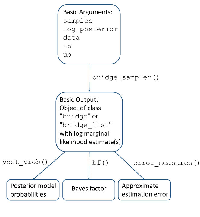
Figure 1: Flow chart of the steps that a user may take when using the bridgesampling package. In general, the user needs to provide a posterior samples object (samples), a function that computes the log of the unnormalized posterior density (log_posterior), the data (data), and parameter bounds (lb and ub). The bridge_sampler function then produces an estimate of the log marginal likelihood. This is usually repeated for at least two different models. The user can then compute posterior model probabilities (using the post_prob function), Bayes factors (using the bf function), and approximate estimation errors (using the error_measures function). Note that the summary method for bridge objects automatically invokes the error_measures function. Figure available at https://tinyurl.com/ybf4jxka under CC license https://creativecommons.org/licenses/by/2.0/.

This allows the user to obtain posterior samples in a convenient and efficient way, for instance, via JAGS (Plummer2003) or a highly customized sampler. Hence, bridge sampling does not require users to program their own MCMC routines to obtain posterior samples; this convenience is usually missing for methods such as Reversible Jump MCMC (but see rjmcmc).

When the model is specified in Stan (CarpenterEtAl2017; rstan) – in a way that retains the constants, as described below – obtaining the marginal likelihood is even simpler: the user only needs to pass the stanfit object to the bridge_sampler function. The combination of Stan and the bridgesampling package therefore produces an unsupervised, black box computation of the marginal likelihood.

This article is structured as follows: First we describe the implementation details of the algorithm from bridgesampling; second, we illustrate the functionality of the package using a simple Bayesian $t$-test example where posterior samples are obtained via JAGS. In this section, we also explain a heuristic to obtain the function that computes the log of the unnormalized posterior density in JAGS; third, we describe in more detail the interface to Stan which enables an even more automatized computation of the marginal likelihood. Fourth, we illustrate use of the Stan interface with two well-known examples from the Bayesian model selection literature.

2 Bridge sampling: the algorithm

Bridge sampling can be thought of as a generalization of simpler methods for estimating normalizing constants such as the naive Monte Carlo estimator, the generalized harmonic mean estimator, and importance sampling (e.g., FruehwirthSchnatter2004; GronauEtAltutorial). These simpler methods typically use samples from a single distribution, whereas bridge sampling combines samples from two distributions. For instance, in its original formulation (MengWong1996), bridge sampling was used to estimate a ratio of two normalizing constants such as the Bayes factor. In this scenario, the two distributions for the bridge sampler are the posteriors for each of the two models involved. However, the accuracy of the estimator depends crucially on the overlap between the two involved distributions; consequently, the accuracy can be increased by estimating a single normalizing constant at a time, using as a second distribution a convenient normalized proposal distribution that closely matches the distribution of interest (e.g., GronauEtAltutorial; OverstallForster2010). The bridge sampling estimator of the marginal likelihood is then given by:

$$p(\bm{y})=\frac{\mathbb{E}_{g(\bm{\theta})}\left[h(\bm{\theta})\,p(\bm{y}\mid\bm{\theta})\,p(\bm{\theta})\right]}{\mathbb{E}_{p(\bm{\theta}\mid\bm{y})}\left[h(\bm{\theta})\,g(\bm{\theta})\right]}\approx\frac{\frac{1}{n_{2}}\sum_{j=1}^{n_{2}}h(\tilde{\bm{\theta}}_{j})\,p(\bm{y}\mid\tilde{\bm{\theta}}_{j})\,p(\tilde{\bm{\theta}}_{j})}{\frac{1}{n_{1}}\sum_{i=1}^{n_{1}}h(\bm{\theta}^{\ast}_{i})\,g(\bm{\theta}^{\ast}_{i})},$$ (5)

where $h(\bm{\theta})$ is called the bridge function and $g(\bm{\theta})$ denotes the proposal distribution. $\{\bm{\theta}^{\ast}_{1},\bm{\theta}^{\ast}_{2},\ldots,\bm{\theta}^{\ast}_{n_{1}}\}$ denote $n_{1}$ samples from the posterior distribution $p(\bm{\theta}\,|\,\bm{y})$ and $\{\tilde{\bm{\theta}}_{1},\tilde{\bm{\theta}}_{2},\ldots,\tilde{\bm{\theta}}_{n_{2}}\}$ denote $n_{2}$ samples from the proposal distribution $g(\bm{\theta})$.

To use bridge sampling in practice, one has to specify the bridge function $h(\bm{\theta})$ and the proposal distribution $g(\bm{\theta})$. For the bridge function $h(\bm{\theta})$, the bridgesampling package implements the optimal choice presented in MengWong1996 which minimizes the relative mean-squared error of the estimator. Using this particular bridge function, the bridge sampling estimate of the marginal likelihood is obtained via an iterative scheme that updates an initial guess of the marginal likelihood $\hat{p}(\bm{y})^{(0)}$ until convergence (for details, see MengWong1996; GronauEtAltutorial). The estimate at iteration $t+1$ is obtained as follows:

$$\hat{p}(\bm{y})^{(t+1)}=\frac{\frac{1}{n_{2}}\sum\limits_{j=1}^{n_{2}}\frac{l_{2,j}}{s_{1}\thinspace l_{2,j}+s_{2}\thinspace\hat{p}(\bm{y})^{(t)}}}{\frac{1}{n_{1}}\sum\limits_{i=1}^{n_{1}}\frac{1}{s_{1}\thinspace l_{1,i}+s_{2}\thinspace\hat{p}(\bm{y})^{(t)}}},$$ (6)

where $l_{1,i}=\frac{p(\bm{y}\mid\bm{\theta}^{\ast}_{i})\,p(\bm{\theta}^{\ast}_{i})}{g(\bm{\theta}^{\ast}_{i})}$, and $l_{2,j}=\frac{p(\bm{y}\mid\tilde{\bm{\theta}}_{j})\,p(\tilde{\bm{\theta}}_{j})}{g(\tilde{\bm{\theta}}_{j})}$. In practice, a more numerically stable version of Equation (6) is implemented that uses logarithms in combination with the Brobdingnag R package (Brobdingnag) to avoid numerical under- and overflow (for details, see GronauEtAltutorial, Appendix B).

The iterative scheme usually converges within a few iterations. Note that, crucially, $l_{1,i}$ and $l_{2,j}$ need only be computed once before the iterative updating scheme is started. In practice, evaluating $l_{1,i}$ and $l_{2,j}$ takes up most of the computational time. Luckily, $l_{1,i}$ and $l_{2,j}$ can be computed completely in parallel for each $i\in\left\{1,2,\ldots,n_{1}\right\}$ and each $j\in\left\{1,2,\ldots,n_{2}\right\}$, respectively. That is, in contrast to MCMC procedures, the evaluation of, for instance, $l_{1,i+1}$ does not require one to evaluate $l_{1,i}$ first (since the posterior samples and proposal samples are already available). The bridgesampling package enables the user to compute $l_{1,i}$ and $l_{2,j}$ in parallel by setting the argument cores to an integer larger than one. On Unix/macOS machines, this parallelization is implemented using the parallel package. On Windows machines this is achieved using the snowfall package (snowfall).

After having specified the bridge function, one needs to choose the proposal distribution $g(\bm{\theta})$. The bridgesampling package implements two different choices: (a) a multivariate normal proposal distribution with mean vector and covariance matrix that match the respective posterior samples quantities and (b) a standard multivariate normal distribution combined with a warped posterior distribution. Both choices increase the efficiency of the estimator by making the proposal and the posterior distribution as similar as possible. Note that under the optimal bridge function, the bridge sampling estimator is robust to the relative tail behavior of the posterior and the proposal distribution. This stands in sharp contrast to the importance and the generalized harmonic mean estimator for which unwanted tail behavior produces estimators with very large or even infinite variances (e.g., OwenZhou2000; FruehwirthSchnatter2004; GronauEtAltutorial).

2.1 Option I: the multivariate normal proposal distribution

The first choice for the proposal distribution that is implemented in the bridgesampling package is a multivariate normal distribution with mean vector and covariance matrix that match the respective posterior samples quantities. This choice (henceforth “the normal method”) generalizes to high dimensions and accounts for potential correlations in the joint posterior distribution. This proposal distribution is obtained by setting the argument method = "normal" in the bridge_sampler function; this is the default setting. This choice assumes that all parameters are allowed to range across the entire real line. In practice, this assumption may not be fulfilled for all components of the parameter vector, however, it is usually possible to transform the parameters so that this requirement is met. This is achieved by transforming the original $p$-dimensional parameter vector $\bm{\theta}$ (which may contain components that range only across a subset of $\mathbb{R}$) to a new parameter vector $\bm{\xi}$ (where all components are allowed to range across the entire real line) using a diffeomorphic vector-valued function $f$ so that $\bm{\xi}=f(\bm{\theta})$. By the change-of-variable rule, the posterior density with respect to the new parameter vector $\bm{\xi}$ is given by:

$$p(\bm{\xi}\mid\bm{y})=p_{\bm{\theta}}(f^{-1}(\bm{\xi})\mid\bm{y})\,\left\lvert\det\left[J_{f^{-1}}(\bm{\xi})\right]\right\rvert,$$ (7)

where $p_{\bm{\theta}}(f^{-1}(\bm{\xi})\mid\bm{y})$ refers to the untransformed posterior density with respect to $\bm{\theta}$ evaluated for $f^{-1}(\bm{\xi})=\bm{\theta}$. $J_{f^{-1}}(\bm{\xi})$ denotes the Jacobian matrix with the element in the $i$-th row and $j$-th column given by $\frac{\partial\theta_{i}}{\partial\xi_{j}}$. Crucially, the posterior density with respect to $\bm{\xi}$ retains the normalizing constant of the posterior density with respect to $\bm{\theta}$; hence, one can select a convenient transformation without changing the normalizing constant. Note that in order to apply a transformation no new samples are required; instead the original samples can simply be transformed using the function $f$.

In principle, users can select transformations themselves. Nevertheless, the bridgesampling package comes with a set of built-in transformations (see Table LABEL:tab:transformations), allowing the user to work with the model in a familiar parameterization. When the user then supplies a named vector with lower and upper bounds for the parameters (arguments lb and ub, respectively), the package internally transforms the relevant parameters and adjusts the expressions by the Jacobian term. Furthermore, as will be elaborated upon below, when the model is fitted in Stan, the bridgesampling package takes advantage of the rich class of Stan transformations.

The transformations built into the bridgesampling package are useful whenever each component of the parameter vector can be transformed separately. In this scenario, there are four possible cases per parameter: (a) the parameter is unbounded; (b) the parameter has a lower bound (e.g., variance parameters); (c) the parameter has an upper bound; and (d) the parameter has a lower and an upper bound (e.g., probability parameters). As shown in Table LABEL:tab:transformations, in case (a) the identity (i.e., no) transformation is applied. In case (b) and (c), logarithmic transformations are applied to transform the parameter to the real line. In case (d) a probit transformation is applied. Note that internally, the posterior density is automatically adjusted by the relevant Jacobian term. Since each component is transformed separately, the resulting Jacobian matrix will be diagonal. This is convenient since it implies that the absolute value of the determinant is the product of the absolute values of the diagonal entries of the Jacobian matrix:

$$\left\lvert\det\left[J_{f^{-1}}(\bm{\xi})\right]\right\rvert=\prod_{i=1}^{p}\left\lvert\frac{\partial\theta_{i}}{\partial\xi_{i}}\right\rvert.$$ (8)

Table 1: Overview of built-in transformations in the bridgesampling package. $l$ denotes a parameter lower bound and $u$ denotes an upper bound. $\Phi(\cdot)$ denotes the cumulative distribution function (cdf) and $\phi(\cdot)$ the probability density function (pdf) of the normal distribution.

Type	Transformation	Inv.-Transformation	Jacobian Contribution
unbounded	$\xi_{i}=\theta_{i}$	$\theta_{i}=\xi_{i}$	$\left\lvert\frac{\partial\theta_{i}}{\partial\xi_{i}}\right\rvert=1$
lower-bounded	$\xi_{i}=\log\left(\theta_{i}-l\right)$	$\theta_{i}=\exp\left(\xi_{i}\right)+l$	$\left\lvert\frac{\partial\theta_{i}}{\partial\xi_{i}}\right\rvert=\exp\left(\xi_{i}\right)$
upper-bounded	$\xi_{i}=\log\left(u-\theta_{i}\right)$	$\theta_{i}=u-\exp\left(\xi_{i}\right)$	$\left\lvert\frac{\partial\theta_{i}}{\partial\xi_{i}}\right\rvert=\exp\left(\xi_{i}\right)$
double-bounded	$\xi_{i}=\Phi^{-1}\left(\frac{\theta_{i}-l}{u-l}\right)$	$\theta_{i}=\left(u-l\right)\Phi\left(\xi_{i}\right)+l$	$\left\lvert\frac{\partial\theta_{i}}{\partial\xi_{i}}\right\rvert=\left(u-l\right)\phi\left(\xi_{i}\right)$

Once all posterior samples have been transformed to the real line, a multivariate normal distribution is fitted using method-of-moments. On a side note, bridge sampling may underestimate the marginal likelihood when the same posterior samples are used both for fitting the proposal distribution and for the iterative updating scheme (i.e., Equation (6)). Hence, as recommended by OverstallForster2010, the bridgesampling package divides each MCMC chain into two halves, using the first half for fitting the proposal distribution and the second half for the iterative updating scheme.

2.2 Option II: warping the posterior distribution

The second choice for the proposal distribution that is implemented in the bridgesampling package is a standard multivariate normal distribution in combination with a warped posterior distribution. The goal is still to match the posterior and the proposal distribution as closely as possible. However, instead of manipulating the proposal distribution, it is fixed to a standard multivariate normal distribution, and the posterior distribution is manipulated (i.e., warped). Crucially, the warped posterior density retains the normalizing constant of the original posterior density. The general methodology is referred to as Warp bridge sampling (MengSchilling2002).

There exist several variants of Warp bridge sampling; in the bridgesampling package, we implemented Warp-III bridge sampling (MengSchilling2002; Overstall2010thesis; GronauEtAlwarp3) which can be used by setting method = "warp3". This version matches the first three moments of the posterior and the proposal distribution. That is, in contrast to the simpler normal method described above, Warp-III not only matches the mean vector and the covariance matrix of the two distributions, but also the skewness. Consequently, when the posterior distribution is skewed, Warp-III may result in an estimator that is less variable. When the posterior distribution is symmetric, both Warp-III and the normal method should yield estimators that are about equally efficient. Hence, in principle, Warp-III should always provide estimates that are at least as precise as the normal method. However, the Warp-III method also takes about twice as much time to execute as the normal method; the reason for this is that Warp-III sampling results in a mixture density (for details, see Overstall2010thesis; GronauEtAlwarp3) which requires that the unnormalized posterior density is evaluated twice as often as in the normal method.

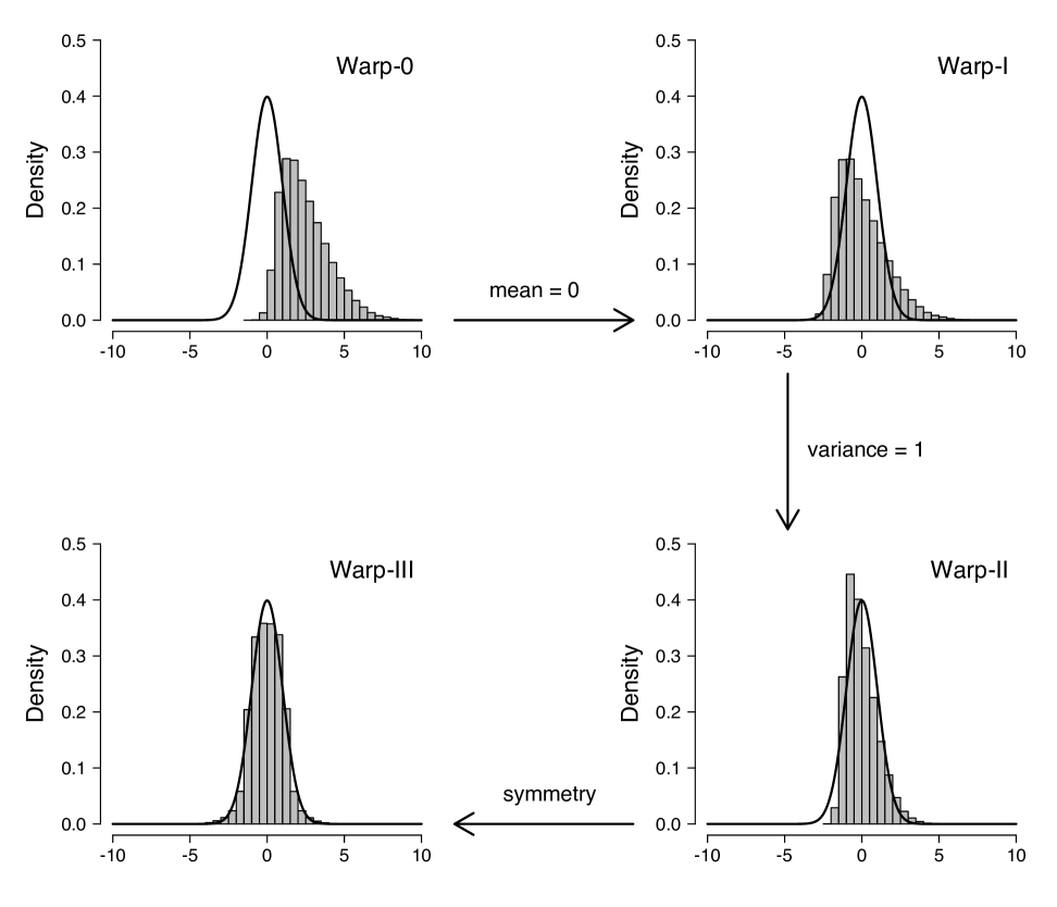
Figure 2: Illustration of the warping procedure. The black solid line shows the standard normal proposal distribution and the gray histogram shows the posterior samples. Available at https://tinyurl.com/y7owvsz3 under CC license https://creativecommons.org/licenses/by/2.0/ (see also GronauEtAlwarp3; GronauEtAlLBA).

Figure 2 illustrates the intuition for the warping procedure in the univariate case. The gray histogram in the top-left panel depicts skewed posterior samples, the solid black line the standard normal proposal distribution. The Warp-III procedure effectively standardizes the posterior samples so that they have mean zero (top-right panel) and variance one (bottom-right panel), and then attaches a minus sign with probability 0.5 to the samples which achieves symmetry (bottom-left panel). This intuition naturally generalizes to the multivariate case. Starting with posterior samples that can range across the entire real line (i.e., $\bm{\xi}$) the multivariate Warp-III procedure is based on the following stochastic transformation:

$$\bm{\eta}=\underbrace{b}_{\textstyle\text{symmetry}}\times\underbrace{\bm{R}^{-1}}_{\textstyle\text{covariance $\bm{I}$}}\times\;\;\underbrace{(\bm{\xi}-\bm{\mu})}_{\textstyle\text{mean $\bm{0}$}},$$ (9)

where $b\sim\mathcal{B}(0.5)$ on $\{-1,1\}$ and $\bm{\mu}$ corresponds to the expected value of $\bm{\xi}$ (i.e., the mean vector). The matrix $\bm{R}$ is obtained via the Cholesky decomposition of the covariance matrix of $\bm{\xi}$, denoted as $\bm{\Sigma}$, hence, $\bm{\Sigma}=\bm{R}\bm{R}^{\top}$. Bridge sampling is then applied using this warped posterior distribution in combination with a standard multivariate normal distribution.

2.3 Estimation error

Once the marginal likelihood has been estimated, the user can obtain an estimate of the estimation error in a number of different ways. One method is to use the error_measures function which is an S3 generic. Note that the summary method for objects returned by bridge_sampler internally calls the error_measures function and thus provides a convenient summary of the estimated log marginal likelihood and the estimation uncertainty. For marginal likelihoods estimated with the "normal" method and repetitions = 1, the error_measures function provides an approximate relative mean-squared error of the marginal likelihood estimate, an approximate coefficient of variation, and an approximate percentage error. The relative mean-squared error of the marginal likelihood estimate is given by:

$$\text{RE}^{2}=\frac{\mathbb{E}\left[\big{(}\hat{p}(\bm{y})-p(\bm{y})\big{)}^{2}\right]}{p(\bm{y})^{2}}.$$ (10)

The bridgesampling package computes an approximate relative mean-squared error of the marginal likelihood estimate based on the derivation by FruehwirthSchnatter2004 which takes into account that the samples from the proposal distribution are independent, whereas the samples from the posterior distribution may be autocorrelated (e.g., when using MCMC sampling procedures).

Under the assumption that the bridge sampling estimator $\hat{p}(\bm{y})$ is unbiased, the square root of the expected relative mean-squared error (Equation (10)) can be interpreted as the coefficient of variation (i.e., the ratio of the standard deviation and the mean). To facilitate interpretation, the bridgesampling package also provides a percentage error which is obtained by simply converting the coefficient of variation to a percentage.

Note that the error_measures function can currently not be used to obtain approximate errors for the "warp3" method with repetitions = 1. The reason is that, in our experience, the approximate errors appear to be unreliable in this case.

There are two further methods for assessing the uncertainty of the marginal likelihood estimate. These methods are computationally more costly than computing approximate errors, but are available for both the "normal" method and the "warp3" method. The first option is to set the repetitions argument of the bridge_sampler function to an integer larger than one. This allows the user to obtain an empirical estimate of the variability across repeated applications of the method. Applying the error_measures function to the output of the bridge_sampler function that has been obtained with repetitions set to an integer large than one provides the user with the minimum/maximum log marginal likelihood estimate across repetitions and the interquartile range of the log marginal likelihood estimates. Note that this procedure assesses the uncertainty of the estimate conditional on the posterior samples, that is, in each repetition new samples are drawn from the proposal distribution, but the posterior samples are fixed across repetitions.

In case the user is able to easily draw new samples from the posterior distribution, the second option is to repeatedly call the bridge_sampler function, each time with new posterior samples. This way, the user obtains an empirical assessment of the variability of the estimate which takes into account both uncertainty with respect to the samples from the proposal and also from the posterior distribution. If computationally feasible, we recommend this method for assessing the estimation error of the marginal likelihood.

After having outlined the underlying bridge sampling algorithm, we next demonstrate the capabilities of the bridgesampling package using three examples. Additional examples are available as vignettes at: https://cran.r-project.org/package=bridgesampling

3 Toy example: Bayesian $t$-test

We start with a simple statistical example: a Bayesian paired-samples $t$-test (Jeffreys1961; RouderEtAl2009Ttest; LyEtAl2016; GronauEtAlarxiv). We use R’s sleep data set (CushnyPeebles1905) which contains measurements for the effect of two soporific drugs on ten patients. Two different drugs where administered to the same ten patients and the dependent measure was the average number of hours of sleep gained compared to a control night in which no drug was administered. Figure 3 shows the increase in sleep (in hours) of the ten patients for each of the two drugs. To test whether the two drugs differ in effectiveness, we can conduct a Bayesian paired-samples $t$-test.

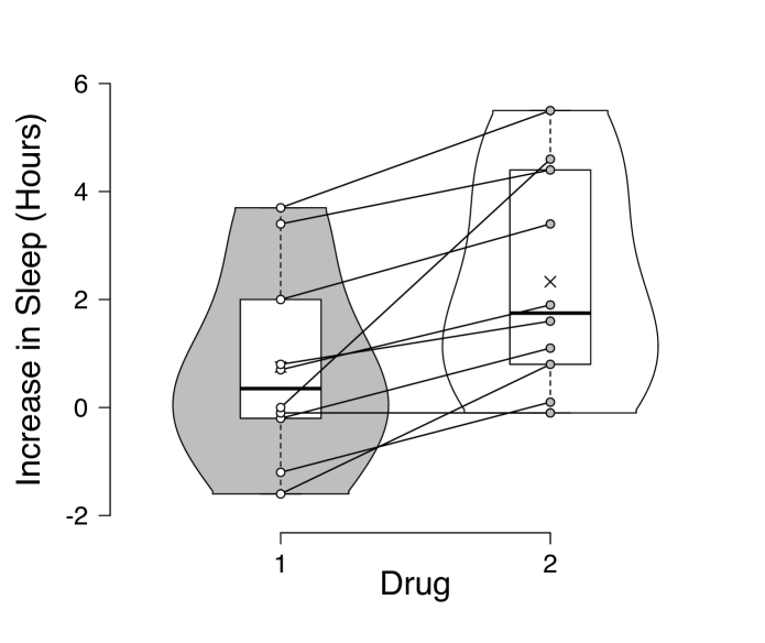
Figure 3: The sleep data set (CushnyPeebles1905). The left violin plot displays the distribution of the increase in sleep (in hours) of the ten patients for the first drug, the right violin plot displays the distribution of the increase in sleep (in hours) of the ten patients for the second drug. Boxplots and the individual observations are superimposed. Observations for the same participant are connected by a line. Figure available at https://tinyurl.com/yalskr23 under CC license https://creativecommons.org/licenses/by/2.0/.

The null hypothesis $\mathcal{H}_{0}$ states that the $n$ difference scores $d_{i},\,i=1,2,\ldots,n$, where $n=10$, follow a normal distribution with mean zero and variance $\sigma^{2}$, that is, $d_{i}\sim\mathcal{N}(0,\sigma^{2})$. The alternative hypothesis $\mathcal{H}_{1}$ states that the difference scores follow a normal distribution with mean $\mu=\sigma\delta$, where $\delta$ denotes the standardized effect size, and variance $\sigma^{2}$, that is, $d_{i}\sim\mathcal{N}(\sigma\delta,\sigma^{2})$. Jeffreys’s prior is assigned to the variance $\sigma^{2}$ so that $p(\sigma^{2})\propto 1/\sigma^{2}$ and a zero-centered Cauchy prior with scale parameter $r=1/\sqrt{2}$ is assigned to the standardized effect size $\delta$ (for details, see RouderEtAl2009Ttest; LyEtAl2016; MoreyRouderBayesFactorPackage).

In this example, we are interested in computing the Bayes factor $\text{BF}_{10}$ which quantifies how much more likely the data are under $\mathcal{H}_{1}$ (i.e., there is a difference between the two drugs) than under $\mathcal{H}_{0}$ (i.e., there is no difference between the two drugs) by using the bridgesampling package. For this example, the Bayes factor can also be easily computed using the BayesFactor package (MoreyRouderBayesFactorPackage), allowing us to compare the results from the bridgesampling package to the correct answer.

The first step is to obtain posterior samples. In this example, we use JAGS in order to sample from the models. Here we focus on how to compute the log marginal likelihood for $\mathcal{H}_{1}$. The steps for obtaining the log marginal likelihood for $\mathcal{H}_{0}$ are analogous. After having specified the model corresponding to $\mathcal{H}_{1}$ as the character string code_H1, posterior samples can be obtained using the R2jags package (R2jags) as follows: R> library("R2jags") R> data("sleep") R> y <- sleep$extra[sleep$group == 1] R> x <- sleep$extra[sleep$group == 2] R> d <- x - y # compute difference scores R> n <- length(d) R> set.seed(1) R> jags_H1 <- jags(data = list(d = d, n = n, r = 1 / sqrt(2)), + parameters.to.save = c("delta", "inv_sigma2"), + model.file = textConnection(code_H1), n.chains = 3, + n.iter = 16000, n.burnin = 1000, n.thin = 1) Note the relatively large number of posterior samples; reliable estimates for the quantities of interest in testing usually necessitate many more posterior samples than are required for estimation. As a rule of thumb, we suggest that testing requires about an order of magnitude more posterior samples than estimation.

Next, we need to specify a function that take as input a named vector with parameter values and a data object, and returns the log of the unnormalized posterior density (i.e., the log of the integrand in Equation (4)). This function is easily specified by inspecting the JAGS model. As a heuristic, one only needs to consider the model code where a “$\sim$” sign appears. The log of the densities on the right-hand side of these “$\sim$” symbols needs to be evaluated for the relevant quantities and then these log density values are summed. Using this heuristic, we obtain the following unnormalized log posterior density function for $\mathcal{H}_{1}$: R> log_posterior_H1 <- function(pars, data) + delta <- pars["delta"] # extract parameter + inv_sigma2 <- pars["inv_sigma2"] # extract parameter + sigma <- 1 / sqrt(inv_sigma2) # convert precision to sigma + out <- + dcauchy(delta, scale = data$r,log=TRUE)+#prior+dgamma(inv_{s}igma2,0.0001,0.0001,log=TRUE)+#prior+sum(dnorm(data$d, sigma * delta, sigma, log = TRUE)) # likelihood + return(out) +

The final step before we can compute the log marginal likelihoods is to specify named vectors with the parameter bounds: R> lb_H1 <- rep(-Inf, 2) R> ub_H1 <- rep(Inf, 2) R> names(lb_H1) <- names(ub_H1) <- c("delta", "inv_sigma2") R> lb_H1[["inv_sigma2"]] <- 0

The log marginal likelihood for $\mathcal{H}_{1}$ can then be obtained by calling the bridge_sampler function as follows: R> library("bridgesampling") R> set.seed(12345) R> bridge_H1 <- bridge_sampler(samples = jags_H1, + log_posterior = log_posterior_H1, + data = list(d = d, n = n, r = 1 / sqrt(2)), + lb = lb_H1, ub = ub_H1) We obtain: R> print(bridge_H1) Bridge sampling estimate of the log marginal likelihood: -27.17103 Estimate obtained in 5 iteration(s) via method "normal". Note that by default, the "normal" bridge sampling method is used.

Next, we can use the error_measures function to obtain an approximate percentage error of the estimate: R> error_measures(bridge_H1)$percentage\Soutput[1]"0.087Thesmallapproximatepercentageerrorindicatesthatthemarginallikelihoodhasbeenestimatedreliably.Asmentionedbefore,wecanusethe\code{summary}methodtoobtainaconvenientsummaryofthebridgesamplingestimateandtheestimationerror.Weobtain:\Sinput R>summary(bridge_{H}1)\Soutput Bridgesamplinglogmarginallikelihoodestimate(method="normal",repetitions=1):\par-27.17103\par ErrorMeasures:\par RelativeMean-SquaredError:7.564225e-07CoefficientofVariation:0.0008697255PercentageError:0.087\par Note:Allerrormeasuresareapproximate.Afterhavingcomputedthelogmarginallikelihoodestimatefor$H_0$inasimilarfashion,wecancomputetheBayesfactorfor$H_1$over$H_0$usingthe\code{bf}function:\Sinput R>bf(bridge_{H}1,bridge_{H}0)\Soutput EstimatedBayesfactorinfavorofbridge_{H}1overbridge_{H}0:17.26001Hence,theobserveddataareabout17timesmorelikelyunder$H_1$(whichassignsthestandardizedeffectsize$δ$azero-centeredCauchypriorwithscale$r = 1/2$)thanunder$H_0$(whichfixes$δ$tozero).Thisisstrongevidenceforadifferenceineffectivenessbetweenthetwodrugs\cite[citep]{(\@@bibref{AuthorsPhrase1Year}{Jeffreys1939}{\@@citephrase{, }}{}, Appendix I)}.TheestimatedBayesfactorcloselymatchestheBayesfactorobtainedwiththe\pkg{BayesFactor}package(i.e.,$BF_10 = 17.259$).\par$

4 A “black box” Stan interface

The previous section demonstrated how the bridgesampling package can be used to estimate the marginal likelihood for models coded in JAGS. For custom samplers, the steps needed to compute the marginal likelihood are the same. What is required is (a) an object with posterior samples; (b) a function that computes the log of the unnormalized posterior density; (c) the data; and (d) parameter bounds. A crucial step is the specification of the unnormalized log posterior density function. For applied researchers, this step may be challenging and error-prone, whereas for experienced statisticians it might be tedious and cumbersome, especially for complex models with a hierarchical structure.

In order to facilitate the computation of the marginal likelihood even further, the bridgesampling package contains an interface to the generic sampling software Stan (CarpenterEtAl2017). Assisted by the rstan package (rstan), this interface allows users to skip steps (b)-(d) above. Specifically, users who fit their models in Stan (in a way that retains the constants, as is detailed below) can obtain an estimate of the marginal likelihood by simply passing the stanfit object to the bridge_sampler function.

The implementation of this “black box” functionality profited from the fact that, just as the bridgesampling package, Stan’s No-U-Turn sampler internally operates on unconstrained parameters (HoffmanGelman2014; stanmanual). The rstan package provides access to these unconstrained parameters and the corresponding log of the unnormalized posterior density. This means that users can fit models with parameter types that have more complicated constraints than those currently built into bridgesampling (e.g., covariance/correlation matrices) without having to hand-code the appropriate transformations.

As mentioned above, in order to use the bridgesampling package in combination with Stan the models need to be implemented in a way that retains the constants. This can be achieved relatively easily: instead of writing, for instance, y   normal(mu, sigma) or y   bernoulli(theta), one needs to write target += normal_lpdf(y | mu, sigma); and target += bernoulli_lpmf(y | theta); That is, one starts with the fixed expression target += which is then followed by the name of the distribution (e.g., normal). The name of the distribution is followed by _lpdf for continuous distributions and _lpmf for discrete distributions. Finally, in parentheses, there is the variable that was to the left of the “ ” sign (here, y), then a “|” sign, and finally the arguments of the distribution. This achieves that the user specifies the log target density (in this case, the log of the unnormalized posterior density) in a way that retains the constants of the involved distributions.

Note that in case the distributions are truncated, the user needs to code the correct renormalization. For instance, a normal distribution with upper truncation at upper is implemented as follows target += normal_lpdf(y | mu, sigma) - normal_lcdf(upper | mu, sigma); where the function normal_lcdf yields the log of the cumulative distribution function (cdf) of the normal distribution. Likewise, a normal distribution with lower truncation at lower is obtained as target += normal_lpdf(y | mu, sigma) - normal_lccdf(lower | mu, sigma); where normal_lccdf yields the log of the complementary cumulative distribution function (ccdf) of the normal distribution (i.e., the log of one minus the cumulative distribution function of the normal distribution). A normal distribution with lower truncation point lower and upper truncation point upper can be implemented as follows: target += normal_lpdf(y | mu, sigma) - log_diff_exp(normal_lcdf(upper | mu, sigma), normal_lcdf(lower | mu, sigma)); where log_diff_exp(a, b) is a numerically more stable version of the operation $\log\left(\exp\left(a\right)-\exp\left(b\right)\right)$. Note that when implementing a truncated distribution, it is of course also important to give the variable of interest the correct bounds. For instance, for the last example where y has a lower truncation at lower and an upper truncation at upper the variable y should be declared as real<lower = lower, upper = upper> y; For more details about how to implement truncated distributions in Stan we refer the user to the Stan manual (stanmanual, section 5.3, “Truncated Distributions”).

In sum, the bridgesampling package enables users to obtain an estimate of the marginal likelihood for any Stan model (programmed to retain the constants) simply by passing the stanfit object to the bridge_sampler function. Next we demonstrate this functionality using two prototypical examples in Bayesian model selection.

4.1 Stan example 1: Bayesian GLMM

The first example features a generalized linear mixed model (GLMM) applied to the turtles data set (JanzenEtAl2000). This data set is included in the bridgesampling package and contains information about 244 newborn turtles from 31 different clutches. For each turtle, the data set includes information about survival status (0 = died, 1 = survived), birth weight in grams, and clutch (family) membership (indicated by a number between one and 31). Figure 4 displays a scatterplot of clutch membership and birth weight. The clutches have been ordered according to mean birth weight. Dots indicate turtles who survived and red crosses indicate turtles who died. This data set has been analyzed in the context of Bayesian model selection before, allowing us to compare the results from the bridgesampling package to the results reported in the literature (e.g., SinharayStern2005; OverstallForster2010).

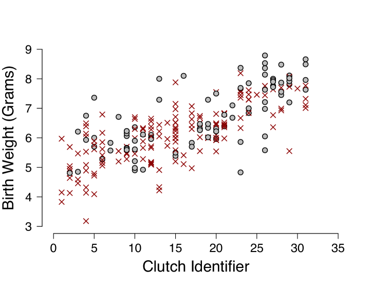
Figure 4: Data for 244 newborn turtles (JanzenEtAl2000). Birth weight is plotted against clutch membership. The clutches have been ordered according to their mean birth weight. Dots indicate turtles who survived and red crosses indicate turtles who died. Figure inspired by SinharayStern2005. Figure available at https://tinyurl.com/yagfxrbw under CC license https://creativecommons.org/licenses/by/2.0/.

Here we focus on the model comparison that was conducted in SinharayStern2005. The data set was analyzed using a probit regression model of the form:

$$\begin{split}y_{i}&\sim\mathcal{B}(\Phi(\alpha_{0}+\alpha_{1}x_{i}+b_{\text{clutch}_{i}})),\hskip 47.80042pti=1,2,\ldots,N\\ b_{j}&\sim\mathcal{N}(0,\sigma^{2}),\hskip 118.0002ptj=1,2,\ldots,C,\end{split}$$ (11)

where $y_{i}$ denotes the survival status of the $i$-th turtle (i.e., 0 = died, 1 = survived), $x_{i}$ denotes the birth weight (in grams) of the $i$-th turtle, $\text{clutch}_{i}\in\{1,2,\ldots,C\},\,i=1,2,\ldots,N$, indicates the clutch to which the $i$-th turtle belongs, $C$ denotes the number of clutches, and $b_{\text{clutch}_{i}}$ denotes the random effect for the clutch to which the $i$-th turtle belongs. Furthermore, $\Phi(\cdot)$ denotes the cumulative distribution function (cdf) of the normal distribution. SinharayStern2005 investigated the question whether there is an effect of clutch membership, that is, they tested the null hypothesis $\mathcal{H}_{0}:\sigma^{2}=0$. The following priors where assigned to the model parameters:

$$\begin{split}\alpha_{0}&\sim\mathcal{N}(0,10),\\ \alpha_{1}&\sim\mathcal{N}(0,10),\\ p(\sigma^{2})&=\left(1+\sigma^{2}\right)^{-2}.\end{split}$$ (12)

SinharayStern2005 computed the Bayes factor in favor of the null hypothesis $\mathcal{H}_{0}:\sigma^{2}=0$ versus the alternative hypothesis $\mathcal{H}_{1}:p(\sigma^{2})=\left(1+\sigma^{2}\right)^{-2}$ using different methods and they reported a “true” Bayes factor of $\text{BF}_{01}=1.273$ (based on extensive numerical integration). Here we examine the extent to which we can reproduce the Bayes factor using the bridgesampling package.

After having implemented the Stan models as character strings H0_code and H1_code, the next step is to run Stan and obtain the posterior samples: R> library("bridgesampling") R> library("rstan") R> data("turtles") R> set.seed(1) R> stanfit_H0 <- stan(model_code = H0_code, + data = list(y = turtles$y,+x=turtles$x, N = nrow(turtles)), + iter = 15500, warmup = 500, + chains = 4, seed = 1) R> stanfit_H1 <- stan(model_code = H1_code, + data = list(y = turtles$y,+x=turtles$x, N = nrow(turtles), + C = max(turtles$clutch),+clutch=turtles$clutch), + iter = 15500, warmup = 500, + chains = 4, seed = 1)

With these Stan objects in hand, estimates of the log marginal likelihoods are obtained by simply passing the objects to the bridge_sampler function: R> set.seed(1) R> bridge_H0 <- bridge_sampler(stanfit_H0) R> bridge_H1 <- bridge