Big-Bang nucleosynthyesis: constraints on nuclear reaction rates, neutrino degeneracy, inhomogeneous and Brans-Dicke models

Abstract

We review the recent progress in the Big-Bang nucleosynthesis which includes the standard and non-standard theory of cosmology, effects of neutrino degeneracy, and inhomogeneous nucleosynthesis within the framework of a Friedmann model. As for a non-standard theory of gravitation, we adopt a Brans-Dicke theory which incorporate a cosmological constant. We constrain various parameters associated with each subject。

PACS Nos.:98.80.-k; 26.35.+c; 98.80.Ft

1 Introduction

Big-Bang nucleosynthesis (BBN) is one of the best astrophysical sites to understand the origin of the light elements,[1] because it produces the primordial abundances of ⁴He, D and ⁷Li [3, 4]. The simplest and most trustful theory is called the standard Big-Bang nucleosynthesis (SBBN), where we assume the cosmological principle that the universe is homogeneous and isotropic in a large scale[2]. Unfortunately, current situation of SBBN is incompatible with the observed abundance of ⁷Li, although it has been pointed out that observational determinations of the ⁷Li abundance contain uncertainties associated with an adopted atmospheric model of metal-poor stars[5] or some unknown physical processes[6].

On the other hand, heavy element nucleosynthesis beyond the mass number $A=8$ has been investigated in a framework of inhomogeneous BBN (IBBN)  [8, 9, 10, 13, 11, 12]. The baryon inhomogeneity could be originated from baryogenesis[12] or some phase transitions [13, 14] which occur as the universe cools down during the expansion. It should be noted that IBBN motivated by QCD phase transition encounters difficulty, because the transition has been proved to be crossed over by the Lattice QCD simulations[16], which means that the phase transition occurs smoothly between the quark-gluon plasma and hadron phase under the finite temperature and zero chemical potential. Although a large scale inhomogeneity of baryon distribution should be ruled out by cosmic microwave background (CMB) observations [17, 18], small scale inhomogeneities are still allowed within the present accuracy of observations. Therefore, it is possible for IBBN to occur in some degree during the early era.

Considering recent progress in observations for peculiar abundance distributions, it is worthwhile to re-investigate IBBN[21, 76, 77] It has been found that[23] synthesis of heavy elements for both $p$- and $r$-processes is possible if $\eta>10^{-4}$ and that the high $\eta$ regions are compatible with the observations of the light elements, ⁴He and D. However, the analysis is only limited to a parameter of a specific baryon number concentration, and a wider possible parameter region should be considered. Therefore we adopt a two-zone model and derive constraints comparing the BBN result with available observations.

In the meanwhile, whole validity of general relativity has not been proved. For example, some kinds of scalar fields may exist in the present epoch. Therefore, we need to examine whether a possibility for a non-standard theory of gravitation survives from the viewpoint of BBN. Simple version of a scalar field theory is the Brans-Dicke theory which include a scalar field. This theory leads to a variation of the gravitational constant and induces an acceleration of the universe. Therefore, we show compatibility between the observations of light elements and the Brans-Dicke theory with a $\Lambda$ term.

In section 2, we give the framework of SBBN and present a detailed comparison among observations and Big-Bang nucleosynthesis in section 3. As an approach to explain a wide range of observational He abundances, we give the effects of neutrino degeneracy on the production of He in section 4. Section 5 is devoted to nucleosynthesis with use of a simple approach for the inhomogeneous BBN. Finally, we give non-standard BBN based on the Brans-Dicke theory in section 6 which remains a room beyond the general relativity. Section 7 summaries possible variations of BBN.

2 Thermal evolution of the universe

In this section, we summarize the evolution of the standard cosmological model, i.e. Friedmann model based on the cosmological principle or the Friedmann-Robertson-Walker metric,

$$ds^{2}=g_{\mu\nu}dx^{\mu}dx^{\nu}=-dt^{2}+a^{2}(t)\left(\frac{dr^{2}}{1-kr^{2}}+r^{2}d\theta^{2}+r^{2}\sin^{2}{\theta}d\phi^{2}\right),$$

where $a(t),t$, and $k$ are the cosmic scale factor, the cosmic time, and the spatial curvature, respectively. The Friedmann model has been constructed with use of the Einstein equation,

$$R_{\mu\nu}-\frac{1}{2}g_{\mu\nu}R=8\pi GT_{\mu\nu}.$$

Here $R_{\mu\nu},R,G$ and $T_{\mu\nu}$ are the Ricci tensor, the scalar curvature, the gravitational constant, and the energy-momentum tensor of the perfect fluid written as $T_{\mu\nu}=pg_{\mu\nu}+(p+\rho)u_{\mu}u_{\nu}$, where $p$ is the pressure, $\rho$ is the energy density, and $u_{\mu}$ is the four velocity.

In practice, we can follow the evolution of temperature $T$ and energy density $\rho$ by solving the Friedmann equation

$$H^{2}\equiv\left(\frac{\dot{a}}{a}\right)^{2}=\frac{8\pi G}{3}\rho-\frac{k}{a^{2}},$$ (1)

where $H$ is called as the Hubble parameter. The total energy density $\rho$ is written as

$$\rho=\rho_{\gamma}+\rho_{\nu}+\rho_{e^{\pm}}+\rho_{b}+\rho_{\rm DM}+\rho_{\Lambda},$$

where the subscripts $\gamma,~{}\nu,~{}e^{\pm},~{}b,~{}{\rm DM}$ and $\Lambda$ indicate photons, neutrinos, electrons and positrons, baryons, dark matter, and the vacuum energy, respectively.

The energy conservation law, ${T^{\mu\nu}}_{;\mu}=0$, reduces to

$$\frac{d}{dt}(\rho a^{3})+p\frac{d}{dt}(a^{3})=0.$$ (2)

The equation of state is described as

$${p}/{\rho}=\begin{cases}1/3&\text{for photons and neutrinos,}\\ 0&\text{for baryons and dark matter,}\\ -1&\text{for vacuum energy.}\end{cases}$$

Therefore, we obtain the evolution of the energy density as $\rho_{b}$ and $\rho_{\rm DM}\propto a^{-3}$, and $\rho_{\gamma,\nu}\propto a^{-4}$. The temperature varies as $T_{\gamma}\propto a^{-1}$ except for the era of the significant entropy transfer from $e^{\pm}$ to photons at $T\simeq 5\times 10^{9}$ K.

Usually, the present values of the energy densities are expressed as the density parameter $\Omega_{i}=\rho_{i,0}/\rho_{cr}$ for $i=\gamma,\nu,b$, DM, and $\Lambda$ with the critical density $\rho_{cr}=3H^{2}_{0}/8\pi G$. Here the subscript $0$ means the value at the present time.

For the baryon density, we also use the baryon-to-photon ratio $\eta$,

$$\eta\equiv\frac{n_{b}}{n_{\gamma}}=2.74\times 10^{-8}\Omega_{b}h^{2},$$ (3)

where $h$ is the dimensionless Hubble constant: $h=H_{0}/100$ [km/s/Mpc]. The value of $\eta$ is kept constant after the electron-positron pair annihilation, because the number densities of photons $n_{\gamma}$ and baryon $n_{b}$ vary as $n_{\gamma}$ and $n_{b}\propto a^{-3}$. From the results of observation of CMB by the Planck satellite, $0.02180<\Omega_{b}h^{2}<0.02272$ at $95$% confidence levels (C.L.) [50], we obtain the range

$$5.96<\eta_{10}<6.22$$ (4)

where $\eta_{10}=\eta/10^{-10}$.

3 Standard Big-Bang nucleosynthesis

3.1 Physical process of the Big-Bang nucleosynthesis

In this section, we describe the standard model of BBN. At the stage $T>10^{10}$ K, photons, neutrinos, and electron (plus positron) are dominant. The energy density is written as follows:

$$\rho=\frac{\pi^{2}k^{4}_{\rm B}}{30\hbar^{3}}\left(2+\frac{7}{2}+\frac{7}{4}N_{\nu}\right)T^{4},$$

where $k_{\rm B}$, $\hbar$, and $N_{\nu}$ are the Boltzmann constant, the Planck constant reduced by $2\pi$, and the effective number of neutrinos (we fixed the value $N_{\nu}=3$). The first, second, and third terms are contributions of photons, electrons and positrons, and neutrinos, respectively. From Eq.(1), the expansion rate of the Universe is $H\sim G^{1/2}T^{2}$. At that time, neutrons and protons are coupled through the weak interaction as follows:

$$n+e^{+} \longleftrightarrow p+\bar{\nu}_{e},$$

$$n+\nu_{e} \longleftrightarrow p+e^{-},$$ (5)

$$n \longleftrightarrow p+e^{-}+\bar{\nu}_{e}$$

The rate of the weak interaction $\Gamma_{wk}$ can be written as $\Gamma_{wk}\sim G_{F}T^{5}$. Here $G_{F}$ is the Fermi coupling constant. The number ratio of the neutrons to protons is written as

$$\frac{n_{n}}{n_{p}}=\exp{\left(-\Delta m/k_{\rm B}T\right)},$$ (6)

where $\Delta m$ is the mass difference between the neutron and proton: $\Delta m=m_{n}-m_{p}=1.29$ MeV.

When $\Gamma_{wk}\simeq H$ at $k_{\rm B}T\simeq 1$ MeV, the ratio (6) is frozen (except for neutron’s $\beta$-decay) and the ratio of the neutrons and protons is fixed to be $1/7$. The ratio in this epoch is very important. As shown later, the most abundant nuclide except for ¹H in the BBN epoch is ⁴He. The abundance of ⁴He is defined by the ratio as follows:

$$Y_{\rm p}=\frac{\rho_{{}^{4}\rm He}}{\rho_{b}}\sim\frac{2n_{n}}{n_{p}+n_{n}}\sim 0.25$$

where $Y_{\rm p}$ is the mass fraction of ⁴He.

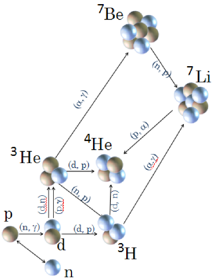
Figure 1: Nuclear reaction network in Big-bang nucleosynthesis.

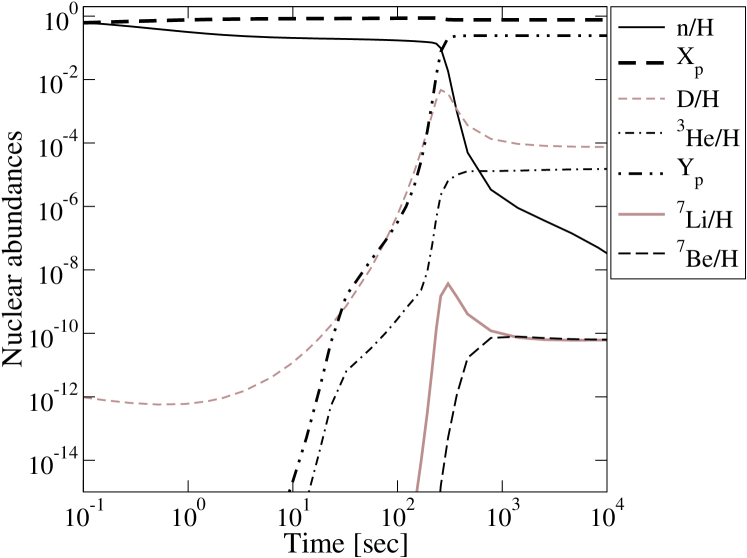
Figure 2: Evolution of mass fractions of ¹H ($X_{\rm p}$) and ⁴He ($Y_{\rm p}$) and number abundances of other nuclides in SBBN.

When the temperature reaches to $0.1$ MeV, the synthesis of light elements starts by the neutron capture reaction of protons: n + p $\longrightarrow$ D $+\gamma$. Figure 1 illustrates the 12 important reactions of BBN.

Figure 2 shows the numerical result of BBN with $\eta_{10}=6.19$ and the neutron life time $\tau_{\rm n}=880.1$ sec[51]. In the BBN era, the heavy element such as CNO cannot be synthesized, because there are no stable element of the mass number $A=5$ and $A=8$. In Fig. 3 we show the produced final values of $Y_{\rm p}$, D/H and ⁷Li/H as a function of $\eta$. The line widths for individual elements correspond to the errors attached to the nuclear reaction rates of NACRE II[53] . Although a new decay rate of free neutrons $\tau_{\rm n}=880.1\pm 1.1$ sec yields[51] $Y_{\rm p}\simeq 0.245$, we adopt the conservative rate considering the uncertainty of the half life.[30]. When the baryon density is high, more D can be synthesized from neutrons and protons. However, reactions which yield helium also begin. As a result, ⁴He increases while D decreases as shown in Fig. 3. We note that the ⁷Li abundance decreases with increasing $\eta$ for $\eta_{10}<3.0$. For $\eta_{10}>3.0$, the tendency becomes opposite. For high baryon density, ⁷Be can be synthesized through ⁴He capture reaction on ³He, and consequently, it is converted to ⁷Li through the electron capture reaction after recombination of ⁷Be.

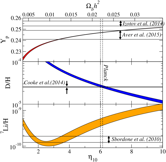
Figure 3: Abundance of light elements produced in SBBN as a function of $\eta$. The vertical region $\Omega_{b}h^{2}=0.02222\pm 0.00023$ indicates the constraint from Planck[50].

3.2 Nuclear reaction rates

To obtain primordial abundances of the light elements numerically shown in Fig.2, it is necessary to solve differential equation of two body reaction for a number fraction $y_{k}$ as follows:

$$\frac{dy_{k}}{dt}=\sum_{i,j,l}{y_{i}y_{j}[ijkl]}-\sum_{i,j,l}{y_{k}y_{l}[klij]},$$

where $[ijkl]$ means the rates of a thermonuclear reaction: $i+j\rightarrow k+l$. Usually the rate is a function of the baryon density and temperature. The other main channel responsible for BBN is the transformation between n and p. We note that three body reactions can be negligible in SBBN.

For BBN study in these 10 years, the reaction rates given by Descouvemont et al.[52] (DAA) and NACRE II.[53] have been used. The DAA rates are obtained by adopting the $R$-matrix theory so as to fit with the low energy data. The NACRE II rates are the updated version of the NACRE compilation[54] which include the thermonuclear reaction rates obtained experimentally for nuclei with A $\leq$ 16. We compare the BBN results between DAA and NACRE II.

Figure 4 shows the results of BBN calculated by using the reaction rates of DAA and NACRE II. The abundances of ⁴He and D are almost the same. However, ⁷Li by NACRE II is 0.5 % higher than that by DAA. This is because, as shown in Fig.5, the rate of the reaction ³He$(\alpha,\gamma){}^{7}$Be of NACRE II is higher than that of DAA at the temperature range of BBN.

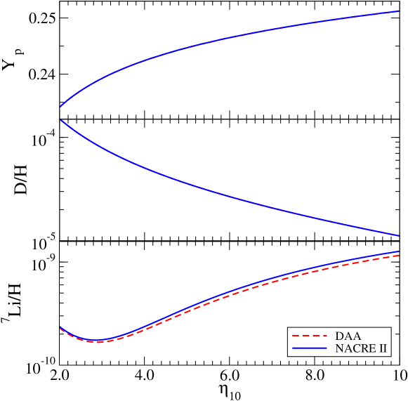
Figure 4: Produced abundances of light elements. The solid curves are calculated from the rates of NACRE II and the dashed ones are of DAA.

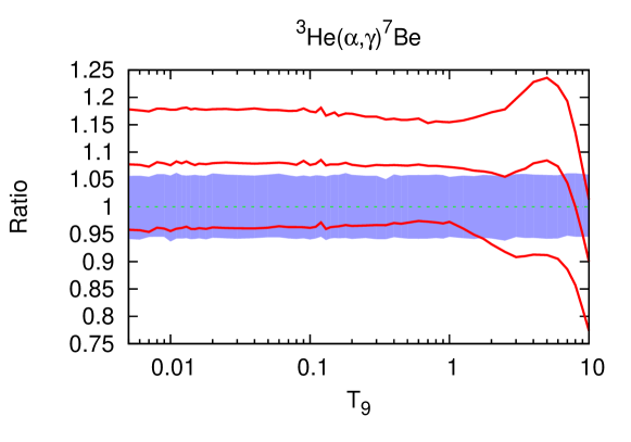
Figure 5: Rates of ³He ($\alpha,\gamma$)⁷Be from NACRE II relative to DAA (adopted value). The horizontal axis means the temperature normalized by $10^{9}$ K. The shaded area indicates the uncertainty of the reaction rate by DAA. The red curves correspond to the high (upper curve) adopted (middle curve) and low (lower curve) values of reaction rates in NACRE II, respectively.

3.3 Constraints from observations of ⁴He, D, and ${}^{7}Li$

The observation of ⁴He is important to constrain physics of the early universe, because the theoretical value of ⁴He is sensitive to cosmological models, such as the gravitational model beyond general relativity and effective neutrino number.

Helium-4 is the most abundant element nuclide except for ¹H produced in BBN. It is also yielded through hydrogen burning inside stars. Since the abundance of ⁴He grows after BBN era, its observed value is an upper limit to the primordial abundance. Thence, it is not easily to determine primordial $Y_{\rm p}$. However, it is deduced that primordial ⁴He remains in a low-metallicity region, because star formation does not occur there.　 Then ⁴He is determined from the recombination lines of proton and helium in extragalactic HII regions.

Recently, observational abundance of ⁴He has a conflict between two groups. Izotov et al. report

$$Y_{\rm p}=0.254\pm 0.003$$ (7)

using linear relation $Y-$O/H for 111 highest-excitation HII regions[44]. And adding the HeI $\lambda$ 10830 Å  emission line, they derived[45]

$$Y_{\rm p}=0.2551\pm 0.0022.$$ (8)

On the other hand, using A Markov Chain Monte Carlo analysis for 93 HII regions, Aver et al.[43] reported

$$Y_{\rm p}=0.2465\pm 0.0097.$$ (9)

Also they reported[46]

$$Y_{\rm p}=0.2449\pm 0.0040.$$ (10)

by evaluating the effects of adding He I $\lambda$10830 infrared emission line in helium abundance determination.

Helium-3 is made from deuteron by D(p,$\gamma$) ³He in the star. Therefore, observations of D give a upper limit of primeval values. Since the abundance of D strongly depends on the baryon density, D is called as “baryometer”. The abundance of D is measured in QSO absorption line system at high-redshift. Recently, the primordial D abundance is determined with a high-accuracy. Pettini & Cooke reported[48]

$$\text{D/H}=(2.535\pm 0.05)\times 10^{-5}.$$ (11)

from the metal-poor damped Lyman $\alpha$ (DLA) system at $z=3.05$. And Cooke et al. reported[47]

$$\text{D/H}=(2.53\pm 0.04)\times 10^{-5}.$$ (12)

from the very metal-poor DLA toward SDSS J1358+6522.

The primeval abundance of ⁷Li can be estimated from observations of Population II stars in our galaxy. In the old galaxy, the relation between [Li/H] and [Fe/H] becomes constant at a low metallicity star (it is called “Spite-Plateau”). The observed abundance of ⁷Li in Population II stars is given by Sbordone et al.  [49]:

$${\rm{}^{7}Li/H}=\left(1.58\pm 0.31\right)\times 10^{-10}.$$ (13)

To find reasonable values of $\eta_{10}$ which satisfy the consistency between BBN and observed values, we calculate $\chi^{2}$ as follows:

$$\chi^{2}_{i}(\eta)={\frac{\left(Y^{th}_{i}(\eta)-Y^{obs}_{i}\right)^{2}}{{\sigma^{2}_{th,i}}+{\sigma^{2}_{obs,i}}}},$$ (14)

where $Y_{i}$ and $\sigma_{i}$ are the abundances and their uncertainties for elements $i~{}(i=Y_{p},{\rm D},{}^{7}{\rm Li})$, respectively. The value $\sigma_{th,i}$ is obtained from the Monte-Carlo calculations using 1$\sigma$ errors associated with nuclear reaction rates. The observational values, $Y^{obs}_{i}$ and their errors $\sigma_{obs,i}$, are taken from (8), (10), (12), and (13).

Finally, we obtain the range of $\eta_{10}$ with $1\sigma$ C.L. from individual observations:

$$3.28\leq\eta_{10}\leq 7.27 \hskip 14.22636pt\text{from Aver et al.\cite[cite]{[\@@bibref{}{Aver2015}{}{}]}},$$

$$10.1\leq\eta_{10}\leq 18.2 \hskip 14.22636pt\text{from Izotov et al.\cite[cite]{[\@@bibref{}{Izotov2014}{}{}]}},$$

$$6.08\leq\eta_{10}\leq 6.38 \hskip 14.22636pt\text{from Cooke et al.\cite[cite]{[\@@bibref{}{Cooke2014}{}{}]}},$$

$$3.28\leq\eta_{10}\leq 4.40$$ from Sbordone et al.[49]

As against the excellent agreement for D and ⁴He, the discrepancy for ⁷Li is unallowable. This is called ”⁷Li problem”. Since the baryon density is determined precisely from CMB observation by WMAP and/or Planck, this problem is conspicuous more than ever.

To solve this problem, many possibilities have been considered, such as unstable massive particles[74, 75], nuclear reaction rates coupled with other reaction paths[70, 71], and a scalar-tensor theory of gravity [72, 73]. It is noted that the observations of ⁷Li involve uncertain atmospheric models concerning the low metallicity stars[41] .

4 Neutrino degeneracy

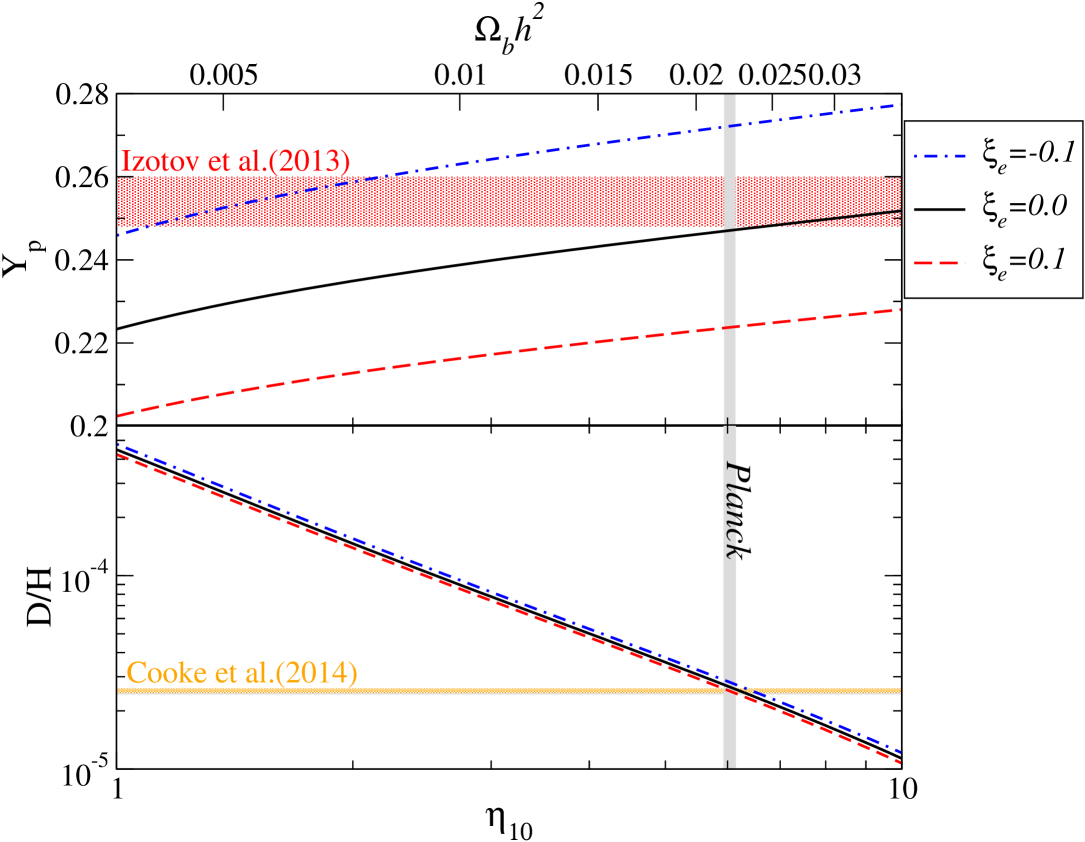
Figure 6: Effects of neutrino degeneracy on the production of ⁴He and D/H. The degeneracy parameters is taken to be $\xi_{\rm e}=-0.1,0$, and $0.1$ from the top to bottom curve. The vertical band comes from the baryon density determined by $Planck$. The horizontal bands correspond to the observational abundances of ⁴He and D/H with $2\sigma$ uncertainty[55].

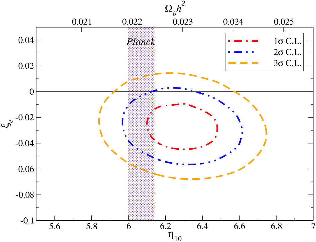
Figure 7: Contours having 1$\sigma$, 2$\sigma$, and 3$\sigma$ confidence levels from $Y_{p}$ and D/H observations in the $\eta_{10}-\xi_{\rm e}$ plane. The horizontal line corresponds to SBBN ($\xi_{e}=0$). The vertical band shows the baryon density from $Planck$[55].

Within the framework of general relativity, BBN can be, for example, extended to include neutrino degeneracy (e.g. Ref. [42]). Degeneracy of electron-neutrinos is described in terms of a parameter

$$\xi_{\rm e}=\mu_{\nu,e}/k_{\rm B}T_{\nu},$$ (15)

where $\mu_{\nu,e}$ is the chemical potential of electron neutrinos and $T_{\nu}$ is the temperature of neutrinos. To get abundance variations of both neutrons and protons caused by nonzero $\xi_{\rm e}$ values, we take a usual method to incorporate the degeneracy into the Fermi-Dirac distribution of neutrinos [42]. In this study, we do not consider the degeneracy of $\tau$- and $\mu$-neutrinos.

In BBN calculations, we implemented the neutrino degeneracy as follows. Before the temperature drops to the difference $\Delta m/k_{\rm B}$ in the rest mass energies between a neutron and a proton, they are in thermal equilibrium through the weak interaction processes (5). Below $k_{\rm B}T=4$ MeV, we solve the rate equations for n and p until $k{}_{\rm B}T$ drops to 1 MeV including the individual weak interaction rates. After that, we begin to operate the nuclear reaction network with the weak interaction rates between n and p included. We should note that in the present parameter range shown below, effects of neutrino degeneracy on the expansion and/or cooling of the universe can be almost neglected, because the absolute values of neutrino degeneracy are rather small, and affect the energy density by at most $10^{-3}\ \%$. (see Fig.7).

The produced amounts of D and ⁷Li are almost the same as those in the SBBN model, respectively, while ⁴He becomes less abundant if $\xi_{\rm e}>0$, since $\beta$-equilibrium leads to lower neutron production. This is because the abundance ratio of neutrons to protons (n/p) is proportional to $\exp[-\xi_{\rm e}]$. This can be seen in Fig.6; while the abundance of ⁴He is very sensitive to $\xi_{\rm e}$, it is insensitive to $\eta$. On the other hand, although the abundance of D is almost uniquely determined from $\eta$, i.e., the nucleon density, it depends weakly on $\xi_{\rm e}$.

To find reasonable values of $\xi_{e}$ and $\eta_{10}$ which satisfy the consistency between BBN and observed ⁴He and D, we calculate $\chi^{2}$ as follows:

$$\chi^{2}(\eta,\xi_{e})=\sum_{i}{\frac{\left(Y^{th}_{i}(\eta,\xi_{e})-Y^{obs}_{i}\right)^{2}}{{\sigma^{2}_{th,i}}+{\sigma^{2}_{obs,i}}}},$$ (16)

where $Y_{i}$ and $\sigma_{i}$ are the abundances and their uncertainties for elements $i~{}(i=Y_{p},{\rm D})$, respectively. The value $\sigma_{th,i}$ is obtained from the Monte-Carlo calculations using 1$\sigma$ errors associated with nuclear reaction rates. The observational values, $Y^{obs}_{i}$ and their errors $\sigma_{obs,i}$, are taken from (9) and (11).

Figure 7 shows the contours enclosing 1$\sigma$, 2$\sigma$, and 3$\sigma$ C.L. in the $\eta_{10}-\xi_{\rm e}$ plane obtained from (16). In consequence, we get the following constraints for both $\eta_{10}$ and $\xi_{\rm e}$[55]:

$$6.17<\eta_{10}<6.38\,\,\,\ \ -3.4\times 10^{-2}<\xi_{\rm e}<-1.8\times 10^{-2}~{}~{}~{}\text{(1$\sigma$ C.L.), }$$ (17)

$$6.02<\eta_{10}<6.54\,\,\,\ -4.6\times 10^{-2}<\xi_{\rm e}<-0.4\times 10^{-2}~{}~{}~{}\text{(2$\sigma$ C.L.).}$$ (18)

It is noted that, except for neutron decay, two-body reactions are dominant during BBN. Only two reaction of the $\beta$-decay of ³H with $\tau_{1/2}=12.32$ y and e-capture of ⁷Be with $\tau_{1/2}=53.24$ d [78] are important weak reactions of light nuclides. These half lives are modified by a small factor through neutrino degeneracy. However, the final abundance is not affected at all.

5 Inhomogeneous Big-Bang nucleosynthesis

5.1 Recent study of inhomogeneous BBN

The study of SBBN has been done under the assumption of the homogeneous universe. On the other hand, BBN with the inhomogeneous baryon distribution also has been investigated. The model is called an inhomogeneous BBN (IBBN). IBBN results from the inhomogeneity of baryon concentrations that could be induced by baryogenesis[12] or phase transitions such as QCD or electro-weak phase transition[7, 8, 9, 10, 11, 14, 15] during the expansion of the universe.

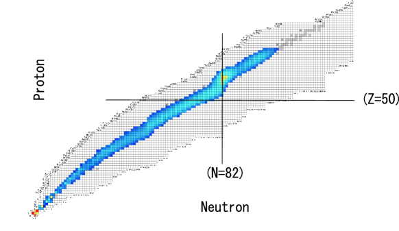
Figure 8: Abundance distribution at $T=3\times 10^{9}$ K with $\eta=10^{-4}$. From Matsuura et al.[24].

A new astrophysical site of BBN is presented[24] that contains very high $\eta$. Figures 8 and 9 show nuclear abundance distributions in a high density region with $\eta=10^{-4}$ on the nuclear chart covering heavy elements. As shown in Fig. 8, stable nuclei are first synthesized. When the temperature goes down, proton- and neutron-capture reactions are active for the nuclei with $A<100$ and with $A>120$, respectively (Fig. 9). Namely, it suggests that both the $r$-process and the $p$-process can occur at the BBN era. On the other hand, for $\eta=10^{-3}$, a proton capture is only active[24]. The problem to be solved is the origin and evolution of the high density region. The size of the high density island is estimated[24] to be $10^{5}-10^{17}$ cm at the BBN epoch. The upper bound is obtained from the maximum angular resolution of CMB and the lower bound is from the analysis[9] of comoving diffusion length of neutrons and protons.

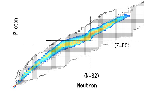
Figure 9: Abundance distribution at $T=10^{9}$ K with $\eta=10^{-4}$[24].

Some models of baryogenesis suggest that very high baryon density regions in the early universe. Recent observations, however, suggest that heavy elements could already exist in high red-shift epochs and therefore the origin of these elements becomes a serious problem. Motivated by these facts, we investigate BBN in very high baryon density regions. The BBN proceeds in proton rich environment, in which a rapid $p$-process is operative.

However, by taking heavy nuclei into account, we find that BBN proceeds through both $p$- and $r$-processes simultaneously. Furthermore, $p$-nuclei such as ⁹²Mo, ⁹⁴Mo, ⁹⁶Ru and ⁹⁸Ru, whose origin is not well known, are also synthesized. The above issues should be refined and checked by investigating the possible model consistent with available observations.

5.2 Two-zone model of IBBN

Quite interesting features[24] have been presented for the possibility of IBBN, but relevant parameters concerning the high and low density regions have not yet been specified. Therefore, we explore the reasonable parameters using a simple two-zone model.[10] The early universe is assumed to contain high and low baryon density regions. For simplicity we ignore the diffusion effects.

We assume that all the produced elements are mixed homogeneously at some epoch between the end of BBN and the recombination era. To construct a two-zone model, we need to define $n_{ave},n_{high}$ and $n_{low}$ as the average-, high-, and low-number densities of baryons, $f_{v}$ as the volume fraction of the high baryon density region, and $X^{ave}_{i},X^{high}_{i}$ and $X^{low}_{i}$ as the mass fractions of element $i$ in the average-, high- and low-density regions, respectively. Then the basic relations between these variables are written as

$$n_{ave} = f_{v}n_{high}+\left(1-f_{v}\right)n_{low},$$ (19)

$$n_{ave}X^{ave}_{i} = f_{v}n_{high}X^{high}_{i}+\left(1-f_{v}\right)n_{low}X^{low}_{i}.$$ (20)

If the baryon fluctuation is assumed to be isothermal[8, 13, 14], the following equations are derived by dividing Eqs. (19) and (20) by the the number density of photons $n_{\gamma}$:

$$\eta_{ave} = f_{v}\eta_{high}+(1-f_{v})\eta_{low},$$ (21)

$$\eta_{ave}X^{ave}_{i} = f_{v}X^{high}_{i}\eta_{high}+(1-f_{v})X^{low}_{i}\eta_{low}.$$ (22)

Here three kinds of $\eta$’s are

$$\eta_{ave}=\frac{n_{ave}}{n_{\gamma}},\qquad\eta_{high}=\frac{n_{high}}{n_{\gamma}},\qquad\eta_{low}=\frac{n_{low}}{n_{\gamma}},$$

where $\eta_{ave}$ is set to be the observed value by CMB[17, 18, 50] : $\eta=6.1\times 10^{-10}$. Both $\eta_{high}$ and $\eta_{low}$ are determined from $f_{v}$ and the density ratio $R=n_{high}/n_{low}=\eta_{high}/\eta_{low}$.

We note that $\rho_{b}$ is the average baryon density obtained from Eq. (19), and temperature $T$ is set to be homogeneous. This assumption is critically important to build our model; otherwise we must treat the zones to evolve separately, which involves fundamental problem as opposed to the cosmological principle.

5.3 Constraints from light element abundances

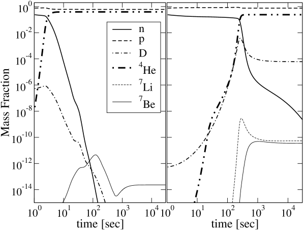
Figure 10: Evolution of light elements in IBBN with $f_{v}=10^{-6}$ and $R=10^{6}$. The left panel corresponds to the high density region $\eta_{high}=3.05\times 10^{-4}$. The right panel corresponds to the low density region $\eta_{low}=3.05\times 10^{-10}$.

We show in Fig. 10 an example of light element synthesis in the high and low density regions with $f_{v}=10^{-6}$ and $R=10^{6}$ that correspond to $\eta_{high}=3.05\times 10^{-4}$ and $\eta_{low}=3.05\times 10^{-10}$. In the right panel for $\eta_{low}$ the evolution of the elements is almost the same as that of SBBN. In the left panel for $\eta_{high}$, D and ⁴He are synthesized at higher temperatures. This is because the reaction ${\rm p}+{\rm n}\longrightarrow{\rm D}+\gamma$ starts at earlier epoch. In addition, the amount of ⁴He is larger than that in the low density region, because neutrons still remain when the nucleosynthesis starts. On the other hand, ⁷Li (or ⁷Be) is much less produced. It implies that heavier nuclei, such as ¹²C and ¹⁶O, are synthesized in the high density region. Using these calculated abundances in both regions, we obtain the average values of the light elements from Eq. (22). Then we can put constraints on $f_{v}$ and $R$ by comparing the values of $Y_{\rm p}$ and D/H with the observed abundances.

In Fig. 11, the constraints are shown in the $f_{v}-R$ plane. Contours of calculated abundances (solid lines) and the $\eta_{high}$ (dashed lines) are drawn. In our analysis, we obtain only the upper limit to the parameter $R$. Note that the allowed region includes density values as high as $\eta_{high}=10^{-3}$.

Since $\eta_{high}$ takes a larger value, nuclei heavier than ⁷Li are synthesized more and more. Then we estimate the abundance of CNO elements in the allowed region. Figure 12 shows the contours of the summation of $X^{ave}_{i}$ over heavier nuclei ($A>7$). As far as our small BBN code is concerned[19], the total mass fraction of CNO nuclei amounts to $X(A>7)\simeq 10^{-5}$.

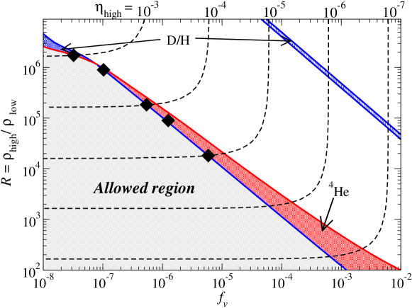
Figure 11: Constraints on the $f_{v}-R$ plane from the observations of ⁴He and D/H. The region below the red line is acceptable region obtained from ⁴He observation by Izotov & Thuan[40] and Aver et al.[58]. Constraints from the D/H observations[56, 48] are shown by the region below the blue lines. The gray region corresponds to the allowable parameters obtained from the two observations of ⁴He and D/H. In the narrow region bounded by two upper blue lines, only the D/H abundance is consistent with observations. This is the contribution of the low density region with $\eta_{low}\sim 10^{-12}$; The D abundance tends to decrease with increasing baryon density for $\eta>10^{-12}$. The dotted lines show the contours of the baryon-to-photon ratio in the high-density region. Filled squares indicate the adopted parameters in §5.4[57].

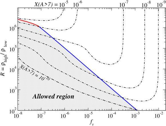
Figure 12: Contours of the total mass fractions of heavier nuclei ($A>7$). The shaded allowed region is the same as in Fig. 9. [57].

5.4 Synthesis of heavy elements in high density region

We investigate synthesis of heavy elements in the high-density region considering the constraints shown in Fig. 11. The abundance change is calculated with a large nuclear reaction network, which contains 4463 nuclei from neutron, proton to Americium (Z = 95 and A = 292). The nuclear data such as reaction rates, nuclear masses and partition functions are the same as used in Ref. 35 except for the weak interaction rates[36] which is adequate for the high temperature stage $T>10^{10}$ K. Note that the mass fractions of ⁴He and D obtained with the large network are consistent with those calculated with a small network in §5.3 within an accuracy of a few percents.

As seen in Fig. 12, heavy elements are produced at the level $X(A>7)\geq 10^{-9}$ in the upper region of $R$ in the allowed region. To examine the efficiency of the heavy element production, we select five models with parameters $\eta_{high}=10^{-3},5.1\times 10^{-4},10^{-4},5.0\times 10^{-5}$ , and $10^{-5}$ which correspond to $\left(f_{v},R\right)=\left(3.24\times 10^{-8},1.74\times 10^{6}\right)$ , $\left(1.03\times 10^{-8},9.00\times 10^{5}\right)$ , $\left(5.41\times 10^{-7},1.84\times 10^{5}\right)$ , $\left(1.50\times 10^{-6},9.20\times 10^{4}\right)$ , and $\left(5.87\times 10^{-6},1.82\times 10^{4}\right)$, respectively. Adopted parameters are indicated by the filled squares in Fig. 11.

Mass fractions of light elements for the two cases : $\eta_{high}\simeq 10^{-3}$, $\eta_{high}=5\times 10^{-4}$. $f_{v},R$ $3.23\times 10^{-8},1.74\times 10^{6}$ $1.03\times 10^{-7},9.00\times 10^{5}$ $(\eta_{high},\eta_{low})$ ($1.02\times 10^{-3}$, $5.86\times 10^{-10}$) ($5.10\times 10^{-4}$, $5.67\times 10^{-10}$) elements high low average high low average p $0.586$ $0.753$ $0.744$ $0.600$ $0.753$ $0.740$ D $1.76\times 10^{-21}$ $4.50\times 10^{-5}$ $4.26\times 10^{-5}$ $3.43\times 10^{-21}$ $4.75\times 10^{-5}$ $4.34\times 10^{-5}$ ³He+T $2.91\times 10^{-14}$ $2.18\times 10^{-5}$ $2.07\times 10^{-5}$ $2.77\times 10^{-14}$ $2.23\times 10^{-5}$ $2.04\times 10^{-5}$ ⁴He $0.413$ $0.247$ $0.256$ $0.400$ $0.247$ $0.260$ ⁷Li+⁷Be $1.63\times 10^{-13}$ $1.78\times 10^{-9}$ $1.68\times 10^{-9}$ $6.80\times 10^{-14}$ $1.65\times 10^{-9}$ $1.52\times 10^{-9}$

Mass fractions of light elements for the two cases : $\eta_{high}\simeq 10^{-4}$, and $\eta_{high}=10^{-5}$. $f_{v},R$ $5.41\times 10^{-7},1.84\times 10^{5}$ $5.87\times 10^{-6},1.82\times 10^{4}$ $(\eta_{high},\eta_{low})$ ($1.04\times 10^{-4}$, $5.62\times 10^{-10}$) ($1.02\times 10^{-5}$, $5.59\times 10^{-10}$) elements high low average high low average p $0.638$ $0.753$ $0.742$ $0.670$ $0.753$ $0.745$ D $6.84\times 10^{-22}$ $4.79\times 10^{-5}$ $4.36\times 10^{-5}$ $1.12\times 10^{-22}$ $4.48\times 10^{-5}$ $4.37\times 10^{-5}$ ³He+T $1.63\times 10^{-13}$ $2.23\times 10^{-5}$ $2.04\times 10^{-5}$ $1.49\times 10^{-9}$ $2.25\times 10^{-5}$ $2.03\times 10^{-5}$ ⁴He $0.362$ $0.247$ $0.258$ $0.330$ $0.247$ $0.254$ ⁷Li+⁷Be $7.42\times 10^{-13}$ $1.64\times 10^{-9}$ $1.49\times 10^{-9}$ $6.73\times 10^{-8}$ $1.62\times 10^{-9}$ $7.96\times 10^{-9}$

Tables 5.4 and 5.4 give the abundance of light elements in the high and low density regions. The mass fractions in the low density region are the same as those obtained in § 5.3, because the abundance flows beyond $A=7$ are negligible. We should note that the averages of abundances $Y_{\rm p}$ and D/H in the two regions coincide with the observed abundances, respectively.

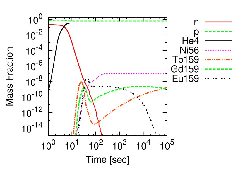
(a) $\eta_{high}=1.02\times 10^{-4}$

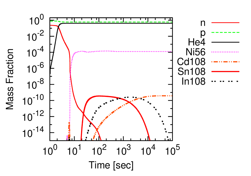
(b) $\eta_{high}=1.06\times 10^{-3}$

Figure 13: Time evolution of the mass fractions in high-density regions of (a) $\eta_{high}=1.02\times 10^{-4}$ and (b) $\eta_{high}=1.06\times 10^{-3}$, respectively.

Figure 13(a) shows the result of nuclsosynthesis in the high density region of $\eta_{high}=1.04\times 10^{-4}$. The nucleosynthesis paths proceed along the stability line during a few seconds, and afterwards they are classified with the mass number. For nuclei with $A\leq 100$, proton captures become very active compared to neutron capture at $T>2\times 10^{9}$ K and the path shifts to the proton rich side, which begins from breaking out the hot CNO cycle. For nuclei of $100<A<120$, the path goes across the stable nuclei from proton- to neutron-rich side, since temperature decreases and the number of seed nuclei of neutron capture increases significantly. Neutron captures become much more efficient for heavier nuclei of ${\it A}\geq 120$. The neutron capture is not similar to the canonical $r-$process, since the nuclear reactions proceed under the condition of the high-abundance of protons. For example, ¹⁵⁹Tb, ¹⁵⁹Gd and ¹⁵⁹Eu are synthesized through neutron captures. After $t=10^{3}$ sec, we can see $\beta$-decays ¹⁵⁹Eu $\rightarrow\,^{159}$Gd $\rightarrow\,^{159}$Tb, where the half life of ¹⁵⁹Eu and ¹⁵⁹Gd are $18.1$ min and $18.479$ h[78], respectively.

The results of $\eta_{high}=1.06\times 10^{-3}$ is shown in Fig.13 (b). The reactions also first proceed along the stability line in the high density region. Subsequently, the reactions directly proceed to the proton-rich side through rapid proton captures. We can see $\beta$-decays ¹⁰⁸Sn $\rightarrow\,^{108}$In $\rightarrow\,^{108}$Cd, where the half life of ¹⁰⁸Sn and ¹⁰⁸In are $10.3$ min and $58.0$ min[78], respectively. In addition, radioactive nuclei ⁵⁶Ni $(\tau_{1/2}=6.075$ d[78]) and ⁵⁷Co ($\tau_{1/2}=271.75$ d[78]) are produced just after the formation of ⁴He in the extremely high density region with $\eta_{high}\geq 10^{-3}$ like the beginning of supernova explosions. [37]

Figure 14 shows the comparison between the average mass fraction produced in IBBN calculation and the solar system abundances by Anders & Grevesse[38]. There are over-produced elements around $A=150$ ($\eta_{high}=10^{-4}$) and $A=80$ ($\eta_{high}=10^{-3}$). Although it seems to conflict with the chemical evolution in the universe, this problem could be solved by the careful choice of $f_{v}$ and/or $R$.[57]

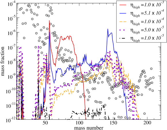
Figure 14: Comparison of the averaged mass fractions in the two-zone model with the solar system abundances [38] (indicated by large dots).[62]

In IBBN model, the lithium-7 can be synthesized in both regions depending on $f_{v}$ and $R$ as shown in Tables 5.4 and 5.4. For $\eta_{high}=1.0\times 10^{-5}$, the averaged value of ⁷Li/H is $1.5\times 10^{-9}$, which is higher than the predicted value in SBBN with $\eta_{10}=6.1$. On the other hand, in cases of $\eta_{high}=5.1\times 10^{-4}$ and $1.0\times 10^{-4}$, the average of ⁷Li/H is lower than the SBBN value. Although these ⁷Li/H values is still higher than the results of recent observation (13) , there remains possibility to solve the “Lithium problem” by extending our IBBN model to another kind of model such a multi-zone model.

6 Brans-Dicke cosmology with a variable cosmological term

6.1 Field equation

The action in the Brans Dicke theory modified with a variable cosmological term $\Lambda$ (BD$\Lambda$) which is a function of a scaler field $\phi$, is given by Endo & Fukui [59] as

$$S=\int d^{4}x\sqrt{-}g\left[\left(R-2\Lambda\right)\phi-\frac{\omega}{\phi}\phi_{,\nu}\phi^{,\nu}+16\pi L_{m}\right],$$ (23)

where $R$, $L_{m}$ and $\omega$ are the scalar curvature, the Lagrangian density of matter , and the dimensionless constant of Brans-Dicke gravity, respectively. The field equations for $BD\Lambda$ are written as follows[60]:

$$R_{\mu\nu}-\frac{1}{2}g_{\mu\nu}R+g_{\mu\nu}\Lambda = \frac{8\pi}{\phi}T_{\mu\nu}+\frac{\omega}{\phi^{2}}\left(\phi_{,\mu}\phi_{,\nu}-\frac{1}{2}g_{\mu\nu}\phi_{,\alpha}\phi^{,\alpha}\right)$$ (24)

$$+\frac{1}{\phi}\left(\phi_{,\mu;\nu}-g_{\mu\nu}\Box\phi\right),$$

$$R-2\Lambda-2\phi\frac{\partial\Lambda}{\partial\phi}=\frac{\omega}{\phi^{2}}\phi_{,\nu}\phi^{,\nu}-\frac{2\omega}{\phi}\Box\phi,$$ (25)

where $\Box$ is the d’Alembertian.

The expansion is described by the following equation derived from the $(0,0)$ component of Eq. (24):

$$\left(\frac{\dot{a}}{a}\right)^{2}=\frac{8\pi\rho}{3\phi}-\frac{k}{a^{2}}+\frac{\Lambda}{3}+\frac{\omega}{6}\left(\frac{{\dot{\phi}}}{{\phi}}\right)^{2}-\frac{\dot{a}}{a}\frac{{\dot{\phi}}}{{\phi}}.$$ (26)

We adopt the simplest case of the coupling between the scalar and matter field

$$\Box\phi=\frac{8\pi\mu}{2\omega+3}T^{\nu}_{\nu},$$ (27)

where $\mu$ is a constant. Original Brans-Dicke theory is deduced for $\mu=1$.

Assuming a perfect fluid for $T_{\mu\nu}$, Eq. (27) reduces to the following:

$$\frac{d}{dt}\left(\dot{\phi}a^{3}\right)=\frac{8\pi\mu}{2\omega+3}\left(\rho-3p\right)a^{3}.$$ (28)

Then, Eq. (28) is integrated to give

$$\dot{\phi}=\frac{1}{a^{3}}\left[\frac{8\pi\mu}{2\omega+3}\rho_{{m}_{0}}t+B\right],$$ (29)

where $B$ is an integral constant and from now on we use the normalized value of $B$: $B^{*}=B/(10^{-24}{\rm{g\ s\ cm^{-3}}})$.

A particular solution of Eq. (25) is obtained from Eqs. (24) and (27):

$$\Lambda=\frac{2\pi\left(\mu-1\right)}{\phi}\rho_{m_{0}}a^{-3},$$ (30)

where $\rho_{m_{0}}$ is the matter density at the present epoch.

The gravitational “constant” $G$ is expressed as follows,

$$G=\frac{1}{2}\left(3-\frac{2\omega+1}{2\omega+3}\mu\right)\frac{1}{\phi}.$$ (31)

The difference of $G$ between the BD$\Lambda$ and the Friedmann model appear at $0.01~{}{\rm sec}<t<1000$ sec as shown in Fig. 15. It suggests that the expansion rate in the BBN epoch is markedly different.

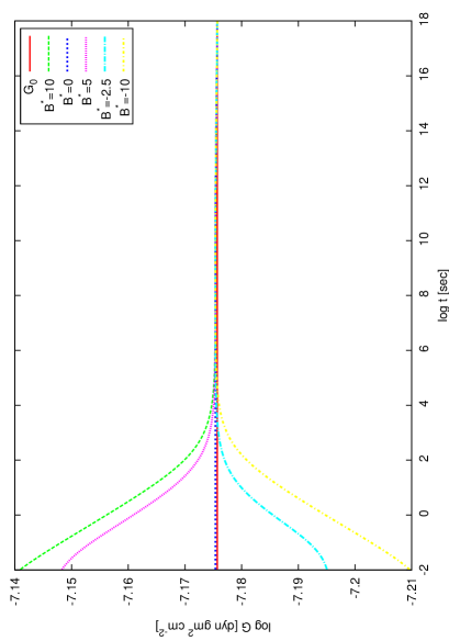
Figure 15: Time evolution of $G$ in BD$\Lambda$ with $\mu=0.6$. $G_{0}$ is the present value: $G_{0}=6.6726\times 10^{-8}~{}{\rm{cm^{3}g^{-1}s^{-2}}}$

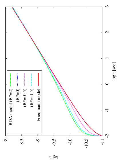
Figure 16: Time evolutions of the scale factor in $BD\Lambda$ with $\mu=0.6$ which are compared to the Friedmann model.

It is reduced to the Friedmann model when $\phi$ = constant and $\omega\gg 1$. Physical parameters have been used to solve Eqs. (26), (29), and (30): $G_{0}=6.6726\times 10^{-8}{\rm{cm^{3}g^{-1}s^{-2}}}$, and $H_{0}=71~{}{\rm{km\ s^{-1}\ Mpc^{-1}}}$.

The parameter $\omega$ is an intrinsic parameter in the Brans-Dicke gravitational model, and it determines the expansion rate of the early universe. In our study, we set $\omega=10000$. Although the variations are limited to the earlier ara, still larger value of $\omega$ can be permitted for our BD$\Lambda$ model (see Fig. 15). Recent observations by the Cassini measurements of the Shapiro time delay suggested that the lower limit of $\omega$ is very large: $\omega\geq 4\times 10^{4}$ (Berti et al.[63], Bertotti et al.[64]).

Figure 16 shows the evolution of the scale factor in $BD\Lambda$ for the several values of $B^{*}$. We identify considerable deviations in $BD\Lambda$ from the Friedmann model at $t<100$ s, which depends on the specific parameters. We note that the evolution of the scale factor depends on both the initial value of $\phi$ and a parameter $\mu$. This is the reason why the scale factor evolves rather differently compared to the Friedmann model.

6.2 Parameter constraints from Big Bang nucleosynthesis

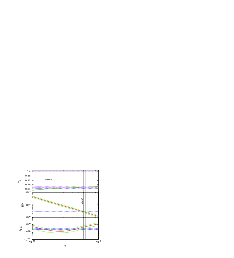
Figure 17: Light element abundances of $\rm{{}^{4}He}$, $\rm{D}$, and $\rm{{}^{7}Li}$ vs. $\eta$ for $B^{*}=2$, $\mu=0.6$, and $\omega=10^{4}$. Dashed lines indicate the $\pm 2\sigma$ uncertainties in nuclear reaction rates in each abundance. The horizontal dotted lines indicate the regions of observational abundances. The solid vertical lines indicate the baryon-to photon ratio $\eta$.

Big-Bang nucleosyntheis provides powerful constraints on possible deviation from the standard cosmology[65]. Changes in the expansion as shown in Fig. 16 affects the abundances of light elements, because the n/p ratio is sensitive to the expansion rate in the BBN epoch.

Figure 17 shows the calculated abundances of $\rm{{}^{4}He}$, $\rm{D}$, and $\rm{{}^{7}Li}$ for $B^{*}=2$ and $\mu=0.6$. The $\pm 2\sigma$ uncertainties in nuclear reaction rates are indicated by the dashed lines. The horizontal dotted lines indicate the observational values of $\rm{{}^{4}He}$, $\rm{D/H}$, and $\rm{{}^{7}Li/H}$ as follows: ${Y_{\rm p}=0.2516\pm 0.0080}$[66], ${Y_{\rm p}=0.326\pm 0.075}$[18], $\rm{D/H=(2.82\pm 0.21)\times 10^{-5}}$ (Pettini et al.[56]), $\rm{{}^{7}Li/H=(2.34\pm 0.32)\times 10^{-10}}$ (Melendez & Ramirez. [67]). Here two observational values of $\rm{{}^{4}He}$ are used. The solid vertical lines indicates the WMAP constraint of the baryon-to-photon ratio, $\rm{\eta=(6.19\pm 0.15)\times 10^{-10}}$ (Komatsu et al.[18]).

The intersection range of the two observational values of $\rm{{}^{4}He}$ is used to constrain the parameters. It is found that the values of $\eta$ derived from $\rm{{}^{4}He}$ and $\rm{D/H}$ are tightly consistent with the value by WMAP, while that from ⁷Li/H is barely consistent. We have a very small parameter region for ⁷Li/H where the bands of the theoretical abundance, the observational abundance, and the WMAP eta overlap. These agreements lead us to the parameter ranges of $0.0\leq~{}\mu\leq 0.6$ and $-2\leq B^{*}\leq 2$.

7 Summary and discussions

We have reviewed the SBBN, BBN with the neutrino degeneracy, IBBN, and BBN in the Brans-Dicke cosmology. First, we have compared the results of SBBN with the current observations of light elements. Considering the uncertainties in the nuclear reaction rates and the observed errors, we can summarize as follows:

1. The consistency is confirmed as far as ⁴He and D are concerned.

2. Large uncertainties of He observations still allow the possibility that some unknown processes beyond SBBN affected the primordial abundance. For example, a large value of $Y_{\rm p}\simeq 0.3$ has been reported in low metallicity stars in globular clusters [40]. This large amount of He could be ascribed to the local neutrino degeneracy.

3. The significant discrepancy concerning ⁷Li remains to be solved.

Second, consistency between IBBN and the observations of ⁴He and D/H abundances has been investigated under the thermal evolution of the standard model with $\eta_{{}_{\rm WMAP}}$. We have examined the two-zone model, where the universe has the high and low baryon density regions separately at the BBN epoch. We have calculated nucleosynthesis that covers 4463 nuclei in the high density region. Below we summarize our results and give some prospects.

1. There are significant differences of the evolution of the light elements between the high and low density regions; In the high density region, nucleosynthesis begins at higher temperature. ⁴He is more abundant than that in the low density region.

2. Both $p$- and $r$-elements are synthesized simultaneously in the high density region with $\eta_{high}\simeq 10^{-4}$. Total mass fractions of nuclides heavier than ⁷Li amount to $10^{-7}$ for $\eta_{high}=10^{-4}$ and $10^{-5}$ for $\eta_{high}=10^{-3}$. The average mass fractions in IBBN are comparable to the solar system abundances.

3. Heavy elements beyond Fe surely affects the formation process of the first generation stars due to the change in the opacity. Therefore, it may be also necessary for IBBN to be constrained from the star formation scenarios.

4. The observed abundances of ⁷Li [49] cannot be explained in terms of SBBN. Although our IBBN model is also inconsistent with ⁷Li observations, the theoretical value of ⁷Li is lower than that of SBBN. Modifications of IBBN model may conduce to the answer.

Third, we show a possible alternate theory of gravity, Brans-Dicke theory with a variable $\Lambda$ term. Even for a very large coupling constant $\omega$, this theory can explain the observed primordial abundances of the light elements. Therefore, it is still worthwhile to continue to explore some non-standard cosmology.

References

-
[1]
R. A. Alpher, H. Bethe and G. Gamow, Phys. Rev. 73 (1948) 803.
C. Hayashi, Prog. Theor. Phys. 5 (1950) 224.
R. V. Wagoner, W. A. Fowler and F. Hoyle, Astrophys. J. 148 (1967) 3. -
[2]
G. Steigman, Ann. Rev. Nucl. Part. Sci. 57 (2007) 463.
F. Iocco et al., Phys. Rept. 472 (2009) 1. -
[3]
V. Luridiana et al., Astrophys. J. 592 (2003) 846.
Y. I. Izotov, T. X. Thuan and G. Stasinska, Astrophys. J. 662 (2007) 15.
D. Kirkman et al., Astrophys. J. Suppl. 149 (2003) 1.
M. Pettini et al., Mon. Not. Roy. Astron. Soc. 391(2008) 1499.
J. M. O’Meara et al., Astrophys. J. 649 (2006) L61. - [4] M. Permbert et al., Astrophys. J. 666 (2007) 636.
-
[5]
S. G. Ryan et al., Astrophys. J. 530 (2000) L57.
P. Bonifacio, et al., Astron. Astrophys. 462 (2007) 851. -
[6]
A. Coc et al., Astrophys. J. 600 (2004) 544.
R. H. Cyburt, B. D. Fields and K. A. Olive, JCAP 0811(2008) 012. -
[7]
K. Jedamzik, and J. B. Rehm, Phys. Rev. D 64 (2001) 023510.;
T. Rauscher et al., Astrophys. J. 429 (1994) 499. - [8] N. Terasawa and K. Sato, Phys. Rev. D 39 (1989) 2893.
- [9] J. H. Applegate, C. J. Hogan and R. J. Scherrer, Phys. Rev. D 35 (1987) 1151.
-
[10]
R. M. Malaney and W. A. Fowler, Astrophys. J. 333 (1988) 14.
J. H. Applegate, C. J. Hogan, R. J. Scherrer, Astrophys. J. 329 (1988) 572.
N. Terasawa and K. Sato, Astrophys. J. 362 (1990) L47.
D. Thomas et al., Astrophys. J. 430 (1994) 291. - [11] K. Jedamzik, G. M. Fuller, G. J. Mathews and T. Kajino, Astrophys. J. 422 (1994) 423.
- [12] S. Matsuura, A. D. Dolgov, S. Nagataki and K. Sato, Prog. Theor. Phys. 112 (2004) 971.
- [13] C. Alcock, G. M. Fuller and G. J. Mathews, Astrophys. J. 320 (1987) 439.
- [14] G. M. Fuller, G. J. Mathews and C. R. Alcock, Phys. Rev. D 37 (1988) 1380.
-
[15]
H. Kurki-Suonio and R. A. Matzner, Phys.Rev. D 39 (1989) 1046.
H. Kurki-Suonio and R. A. Matzner, Phys.Rev. D 42 (1990) 1047. - [16] Y. Aoki et al., Nature 443 (2006) 675.
-
[17]
C.L. Bennett, et al., Astrophys. J. Suppl. 148 (2003) 1.
D. N. Spergel et al., Astrophys. J. Suppl. 170 (2007) 377.
J. Dunkley et al., Astrophys. J. Suppl. 180 (2009) 306. - [18] E. Komatsu et al., Astrophys. J. Suppl. 192 (2011) 47
- [19] M. Hashimoto and K. Arai, Phys. Rep. Kumamoto Univ. 7 (1985) 47
- [20] Y. Juarez et al., Astron. Astrophys. 494 (2009) L25.
- [21] T. Moriya and T. Shigeyama, Phys. Rev. D 81 (2010) 043004.
-
[22]
L. R. Bedin et al., Astrophys. J. 605 (2004) L125.
G. Piotto et al., Astrophys. J. 661 (2007) L53. - [23] S. Matsuura et al., Phys. Rev. D 72 (2005) 123505.
- [24] S. Matsuura et al., Phys. Rev. D 75 (2007) 068302.
- [25] C. Angulo et al., Nucl. Phys. A 656 (1999) 3.
- [26] K. Hagiwara et al., Phys. Rev. D 66 (2002), 010001.
- [27] M. Pettini et al., Mon. Not. Roy. Astron. Soc. 391 (2008) 1499.
- [28] C. Charbonnel and F. Primas, Astron. Astrophys. 442 (2005) 961.
- [29] G. J. Mathews, T. Kajino and T. Shima, Phys. Rev. D 71 (2005) 021302.
-
[30]
A. P. Serebrov et al., Phys. Lett. B 605 (2005) 72.
A. P. Serebrov et al., Phys. Rev. C 78 (2008) 035505. - [31] K. Kohri, M. Kawasaki and K. Sato, Astrophys. J. 490 (1997) 72.
- [32] M. Hashimoto, M. Kamimura and K. Arai, Few–Body Systems Suppl. 12 (2000) 92.
- [33] S. Burles, D. Kirkman and D. Tytler, Astrophys. J. 519 (1999) 18.
- [34] K. Arai, M. Hashimoto and T. Wakita, Phys. Rept. Kumamoto Univ. 11 (2000) 37.
-
[35]
S. Fujimoto et al., Astrophys. J., 585 (2003) 418.
O. Koike, M. Hashimoto, R. Kuromizu and S. Fujimoto, Astrophys. J. 603 (2004) 592.
S. Fujimoto, M. Hashimoto, K. Arai and R. Matsuba, Astrophys. J. 614 (2004) 847.
S. Nishimura et al., Astrophys. J. 642 (2006) 410. - [36] L. Kawano, FERMILAB-Pub-92/04-A
- [37] M. Hashimoto, Prog. Theor. Phys. 94 (1995) 663.
- [38] E. Anders and N. Grevesse, Geochim. Cosmochim. Acta 53 (1989) 197.
- [39] M. Rayet et al., Astron. Astrophys. 298 (1995) 517.
- [40] Y. Izotov and T. X. Thuan, Astrophys. J. 710 (2010) L67.
- [41] A. J. Korn et al., Nature 442 (2006) 657.
- [42] Weinberg, S. 1972, Gravitation and Cosmology: Principles and Applications of the General Theory of Relativity, by Steven Weinberg, pp. 688. ISBN 0-471-92567-5. Wiley-VCH , July 1972.
- [43] E. Aver, K. A. Olive, R. L. Porter and E. D. Skillman, JCAP 1311 (2013) 017.
- [44] Y. I. Izotov, G. Stasinska and N. G. Guseva, Astron. Astrophys. 558 (2013) A57.
- [45] Y. I. Izotov, T. X. Thuan and N. G. Guseva, Mon. Not. Roy. Astron. Soc. 445 (2014) no.1, 778.
- [46] E. Aver, K. A. Olive and E. D. Skillman, JCAP 1507 (2015) no.07, 011.
- [47] R. Cooke, M. Pettini, R. A. Jorgenson, M. T. Murphy and C. C. Steidel, Astrophys. J. 781 (2014) 31.
- [48] M. Pettini, & R. Cooke, Mon. Not. Roy. Astron. Soc. 425 (2012) 2477.
- [49] L. Sbordone et al., Astron. & Astrophys. 522 (2010) A26.
- [50] P. A. R. Ade et al. [Planck Collaboration], arXiv:1502.01589 [astro-ph.CO].
- [51] J. Beringer, J.-F. Arguin, R. M. Barnett, et al. Phys. Rev. D 86 (2012) 010001.
- [52] P. Descouvemont, A. Adahchour, C. Angulo, A. Coc and E. Vangioni-Flam, Atom. Data Nucl. Data Tabl. 88 (2004) 203.
- [53] Y. Xu, K. Takahashi, S. Goriely, M. Arnould, M. Ohta and H. Utsunomiya, Nucl. Phys. A 918 (2013) 61.
- [54] C. Angulo, M. Arnould, M. Rayet et al., Nucl. Phys. A 656 (1999) 3.
- [55] R. Ichimasa, R. Nakamura, M. Hashimoto and K. Arai, Phys. Rev. D 90 (2014) 023527.
- [56] M. Pettini, B. J. Zych, M. T. Murphy, A. Lewis, & C. C. Steidel, Mon. Not. R. Astron. Soc. 391 (2008) 1499.
- [57] R. Nakamura, M. Hashimoto, S. Fujimoto, and K. Sato, J. of Astrophysics vol.2013 Article ID 587294 (2013) 9 pages.
- [58] E. Aver, K. A. Olive, & E. D. Skillman, JCAP 04 (2012) 004.
- [59] M. Endo & T. Fukui, Gen. Rel. Grav. 8 (1977) 833.
- [60] K. Arai, M. Hashimoto, T. Fukui, Astron. & Astrophys. 179 (1987) 17.
- [61] T. Etoh, M. Hashimoto, K. Arai and S. Fujimoto, Astron. & Astrophys. 325 (1997) 893.
- [62] R. Nakamura, M. Hashimoto, S. Gamow, & K. Arai, Astron. & Astrophys. 448 (2006) 23.
- [63] B. Bertotti, L. Iess, & P. Tortora, Nature 425 (2003) 373.
- [64] E. Berti, A. Buonanno, & C. M. Will, Phys. Rev. D, 71, (2005) 084025.
- [65] R. A. Malaney & G. J. Mathews, Phys. Rept. 229 (1993) 145.
- [66] M. Fukugita & M. Kawasaki, Astrophys. J. 646 (2006) 691.
- [67] J. Meléndez,I. & Ramírez, Astrophys. J. 615, (2004) L33.
- [68] R.D. Reasenberg, et al., Astrophysi. J. 234 (1979) L219.
- [69] X. Chen and M. Kamionkowski, Phys. Rev. D 60 (1999) 104036.
- [70] C. Broggini, L. Canton, G. Fiorentini, and F. L. Villante, JCAP, 06 (2012) 030.
- [71] A. Coc, S. Goriely, Y. Xu, M. Saimpert, E. Vangioni, Astrophys. J. 744 (2012) 158.
- [72] A. Coc, K. A. Olive, J. P. Uzan, and E. Vangioni, Phys. Rev. D 73 (2006) 083525.
- [73] J. Larena, J.M. Alimi, and A. Serna, Astrophys. J. 658 (2007) 1.
- [74] M. Kawasaki and M. Kusakabe, Phys. Rev. D 83 (2011) 055011.
- [75] K. Kohri and F. Takayama, Phys. Rev. D 76 (2007) 063507.
- [76] J. F. Lara, T. Kajino and G. J. Mathews, Phys. Rev. D. 73 (2006) 083501.
- [77] P. Vonlanthen et al., Astron. & Astrophy. 503 (2009) 47.
- [78] ENSDF http://www.nndc.bnl.gov/ensdf