On the stability of the $\mu(I)$-rheology for granular flow

Abstract

This article deals with the Hadamard instability of the so-called $\mu(I)$ model of dense rapidly-sheared granular flow, as reported recently by Barker et al. (2015, this journal, 779, 794-818). The present paper presents a more comprehensive study of the linear stability of planar simple shearing and pure shearing flows, with account taken of convective Kelvin wave-vector stretching by the base flow. We provide a closed form solution for the linear stability problem and show that wave-vector stretching leads to asymptotic stabilization of the non-convective instability found by Barker et al. We also explore the stabilizing effects of higher velocity gradients achieved by an enhanced-continuum model based on a dissipative analog of the van der Waals-Cahn-Hilliard equation of equilibrium thermodynamics. This model involves a dissipative hyper-stress, as the analog of a special Korteweg stress, with surface viscosity representing the counterpart of elastic surface tension. Based on the enhanced continuum model, we also present a model of steady shear bands and their non-linear stability against parallel shearing. Finally, we propose a theoretical connection between the non-convective instability of Barker et al. and the loss of generalized ellipticity in the quasi-static field equations. Apart from the theoretical interest, the present work may suggest stratagems for the numerical simulation of continuum field equations involving the $\mu(I)$ rheology and variants thereof.

1 Introduction

Granular flows are ubiquitous in nature and technology, a fact which accounts for a large body of research devoted to the development of continuum models for flows on length scales much larger than the typical grain diameter. Of particular interest here is the phenomenological “$\mu(I)$” model proposed by Jop, Forterre, Pouliquen and coworkers (MiDi, 2004; Jop et al., 2005, 2006), which has proven useful for dense rapidly sheared flows in chutes and avalanching granular layers. However, Barker et al. (2015), hereinafter referred to as Ref.​ 1, conclude that this model is generally ill-posed in the sense of Hadamard, exhibiting the classical linear instability against short wavelength perturbations. We recall that such phenomena are part and parcel of material instability, long recognized in solid mechanics and more recently in the mechanics of complex fluids (See e.g. Goddard, 2003, and references therein ).

While the work of Ref.​ 1 is highly relevant to the modeling of granular flow, particularly as it pertains to numerical simulations, we do not share the authors’ assessment of Hadamard instability as physically “unrealistic”. On the contrary, we assert that this type of instability signals the emergence of spatiotemporal discontinuities, as “weak solutions” of the underlying field equations for numerous physical phenomena, including aerodynamic shocks, hydraulic jumps, thermodynamic phase transitions, and, most relevant to the present work, shear bands or other forms of localized deformation in complex solids and fluids.

In the examples cited above one should distinguish those involving dynamic or “geometric” instability from those representing material instability (Goddard, 2003), a matter discussed further in the following. In either case, numerical simulation generally requires advanced techniques such as shock capturing, adaptive mesh-refinement, or mesh-less methods (cf. Belytschko et al., 1994), to represent certain discontinuous solutions that find widespread applicability in various fields of mechanics and thermodynamics .

Moreover, as particularly appreciated in the field of plasticity (See e.g. Forest & Aifantis, 2010; Henann & Kamrin, 2014), weak solutions may be regularized by means of enhanced continuum models that involve non-local or weakly non-local “gradient” effects. From a physical point of view, such effects represent the emergence of microscopic or mesoscopic length scales or, loosely, “Knudsen effects”. As one of the benefits for numerical simulation, regularization stabilizes against short-wavelength disturbances and imparts a diffuse structure to otherwise sharp discontinuities.

The above considerations provide much of the motivation for the present work whose principal objectives are to:

1. explore a simple gradient regularization of the $\mu(I)$ model, and

2. provide a more complete linear-stability analysis of the regularized model.

For the purposes of Item (1), we shall adopt a visco-plastic tensorial analog of the scalar van der Waals-Cahn-Hilliard (vdW-CH) model of equilibrium thermodynamics, under isothermal conditions, with dissipation potential replacing Helmholtz free energy and with velocity gradient replacing density. We make no claim for the physical validity of this largely phenomenological model of gradient effects, merely noting that it is one of the simplest models imaginable and that it embodies the dissipative analog of a special form of Korteweg stress (Anderson et al., 1998), with surface viscosity arising as the counterpart of equilibrium surface tension. We recall that appeals have been made to the vdW-CH model in the treatment of other dissipative phenomena (e.g. by Forest & Aifantis, 2010), and the thermodynamic version has been connected to microscopic forces by Gurtin (1996). For our purposes, it conveniently elucidates several theoretical issues that have not been sufficiently emphasized in past works.

In the case of Item (2), we shall show that the phenomenon of wave-vector stretching, identified in several previous works (Goddard, 2003) but neglected in the analysis of Ref.​ 1, results in the asymptotic stability of the $\mu(I)$ model, irrespective of the vdW-CH regularization. In effect, initially unstable wave vectors are rotated by simple shearing into an ultimately stable orientation, as foreseen in the path breaking study of hydrodynamic stability by W. Thomson (Thomson, 1887, later Lord Kelvin). To lend a certain plausibility to this scenario, we shall also explore an approximate model of a stable shear band with characteristic thickness derived from the vdW-CH model.

While our stability analysis applies to any homogeneous shear as base state, we shall focus attention here on the two important special cases of planar flows, the simple shear treated in Ref.​ 1 and pure shear .

As a word on notation, we note that, when needed occasionally for clarity, we employ cartesian tensor notation, with sums over repeated indices, with commas denoting partial derivatives, with tensor components indicated in brackets $[\>\>]$, and with occasional listing of vector components in parentheses $(\>\>)$. In coordinate-free notation, the linear transformation of vectors $\mathbf{v}$ into vectors by second-rank tensors $\mathbf{A}$ is denoted by $\mathbf{A}\mathbf{v}=[A_{ij}v_{j}]$, and the special case of the Euclidean scalar product (i.e. ordered contraction) of tensors having equal rank by the standard mathematical “dot” product. We occasionally employ the brackets $[\>\>]$ as standard notation for skew-symmetrization of tensor components and for the arguments of functionals defined on fields.

2 Gradient regularization of $\mu(I)$

As the method we employ applies to general models of viscoplasticity, we offer a derivation of constitutive equation and momentum balance based on the notion of a dissipation potential and the associated hyper-stresses and variational principle. Readers not interested in these details can skip immediately to the momentum balance presented below in (11).

Consider a strictly dissipative material endowed with frame-indifferent dissipation potential (Edelen, 1972, 2005; Goddard, 2014; Saramito, 2016) depending on the first two spatial gradients of the material velocity field $\mathbf{v}(t,\mathbf{x})$:

$$\begin{split}&\psi(\mathbf{D},\nabla\nabla\mathbf{v})=\psi(\mathbf{Q}\mathbf{D}\mathbf{Q}^{T},\mathbf{Q}\nabla\mathbf{Q}\nabla\mathbf{v}\mathbf{Q}^{T}),\\ &\mbox{with}\>\>\mathbf{D}=\frac{1}{2}\left(\nabla\mathbf{v}+(\nabla\mathbf{v})^{T}\right),\end{split}$$ (1)

where $\mathbf{D}$ is the deformation rate and $\mathbf{Q}=\mathbf{Q}(t)$ is an arbitrary time-dependent but spatially independent orthogonal tensor.

A simple special case is represented by the vdW-CH

$$\psi(\mathbf{D},\nabla\nabla\mathbf{v})=\psi_{0}(\mathbf{D})+\chi\left|\nabla\nabla\mathbf{v}\right|^{2},$$ (2)

where we take $\chi$ to be a positive constant, and the term in higher-order velocity gradient $|\nabla\nabla\mathbf{v}|^{2}=(\nabla\nabla\mathbf{v})\!\cdot\!(\nabla\nabla\mathbf{v})=v_{i,jk}v_{i,jk}$ serves to provide a local regularization whenever $\psi_{0}$ becomes locally non-convex. We recall that the gradient term in the standard scalar version of the vdW-CH equation involves fluid density in place of $\nabla\mathbf{v}$ (Cahn & Hilliard, 1958; Gurtin, 1996), providing an energy penalty on large gradients. This yields well- posed field equations in the case of non-convex free-energy with phase transition and serves to define equilibrium surface tension in the limit $\chi\rightarrow 0$.

In the following, we deal with strongly dissipative materials, i.e. strictly dissipative materials devoid of gyroscopic or “powerless” stress (Goddard, 2014), for which the partial derivatives of dissipation potential $\psi(\mathbf{D},\nabla\nabla\mathbf{v})$ yield work-conjugate (symmetric Cauchy) stress $\mathbf{T}^{(1)}$ and hyperstress $\mathbf{T}^{(2)}$, respectively, according to:

$$\mathbf{T}^{(1)}=\frac{\partial\psi}{\partial\mathbf{D}}=\frac{\partial\psi_{0}}{\partial\mathbf{D}}\>\>\mbox{and}\>\>\mathbf{T}^{(2)}=\frac{\partial\psi}{\partial(\nabla\nabla\mathbf{v})}=2\chi\nabla\nabla\mathbf{v}.$$ (3)

and the volumetric rate of dissipation is given by

$$\mathfrak{D}=\mathbf{T}^{(1)}\!\!\cdot\!\mathbf{D}+\mathbf{T}^{(2)}\!\!\cdot\!\nabla\nabla\mathbf{v}=T_{ij}^{(1)}D_{ij}+T_{ijk}^{(2)}v_{k,ij}.$$ (4)

The hyperstress $\mathbf{T}^{(2)}=[T^{(2)}_{ijk}]$ represents a generalized “pinch” $\mathbf{n}\!\cdot\!\mathbf{T}^{(2)}=[n_{i}T^{(2)}_{ijk}]$ acting on a material plane with unit normal $\mathbf{n}$ which can be represented by a force dipole consisting of equal and opposite forces. The symmetric part $[n_{i}T^{(2)}_{i(jk)}]$ involves forces acting along the line of centers of their points of application, representing a normal pinch or symmetric “stresslet”, whereas the antisymmetric part $[n_{i}T^{(2)}_{i[jk]}]$ involves forces acting perpendicular to their line of centers, representing a “torque” or “rotlet”. Note that the gradient of vorticity enters into the mechanical power and that most of the concepts of kinematic and stress carry over from the various works on the elasticity of solids, where strain energy (Helmholtz free energy) rather than dissipation potential is involved.

Thus, upon enslaving micro-structural to continuum kinematics in the classic work of Mindlin (1964), achieved by taking his relative displacement gradient $\gamma_{ij}=0$, one obtains the linear-elastic analog of the present work with his strains $\epsilon_{ij}$ replacing our strain rates $D_{ij}$. Our quasi-static equation of equilibrium (7) follows from that of Mindlin upon relaxing the assumption of incompressibility and combining his Eqs. (4.1), effectively eliminating his “relative stress” $\sigma_{ij}$. Mindlin’s work also shows that, within a linear isotropic gradient model, one may anticipate further quadratic terms in $\nabla\nabla\mathbf{v}$ beyond that adopted in the simpler one-parameter model (2) of the present study.

The Hamiltonian momentum balances for the hyper-elastic system of Mindlin do not apply to hyper-dissipative systems, except in the limit of quasi-static (i.e. inertialess ) motion. Hence, further analysis is required to obtain the relevant balances for the latter, and we begin with the variational principle leading to the quasi-static balance. We note that similar methods have been adopted in past works of Hill (1956) and Leonov (1988), methods which are made rigorous mathematically by the later works of Edelen, e.g. Edelen (1972, 2005), that are highlighted and simplified in the survey by Goddard (2014).

Note that the variational derivative of the functional of $\mathbf{v}(\mathbf{x},t)$ representing global dissipation potential:

$$\Psi[\mathbf{v}]=\int_{V}[\psi(\mathbf{D},\nabla\nabla\mathbf{v})-p\nabla\!\cdot\!\mathbf{v}]\mathop{}\mathrm{d}V,$$ (5)

subject to incompressibility $\nabla\!\cdot\!\mathbf{v}=0$ in spatial domain V, is given by

$$\begin{split}\delta\Psi[\mathbf{v}]&=\int_{V}\left[\frac{\partial\psi}{\partial\mathbf{D}}\!\cdot\!\delta\nabla\mathbf{v}+\frac{\partial\psi}{\partial(\nabla\nabla\mathbf{v})}\!\cdot\!\delta\nabla\nabla\mathbf{v}-p\nabla\!\cdot\!\delta\mathbf{v}\right]\mathop{}\mathrm{d}V\\ &=\int_{V}\left[T_{ij}^{(1)}\delta v_{i,j}+T_{ijk}^{(2)}\delta v_{i,jk}-p\delta v_{j,j}\right]\mathop{}\mathrm{d}V\\ &=\int_{V}\left[(T_{ij}^{(1)}\delta v_{i})_{,j}-T_{ij,j}^{(1)}\delta v_{i}+(T_{ijk}^{(2)}\delta v_{i,j})_{,k}\right.\\ &-\left.(T_{ijk,k}^{(2)}\delta v_{i})_{,j}+T_{ijk,jk}^{(2)}\delta v_{i}-(p\delta v_{j})_{,j}+p_{,j}\delta v_{j}\right]\mathop{}\mathrm{d}V\\ &=\int_{\partial V}\mathbf{n}\!\cdot\!\left[(\mathbf{T}^{(1)}-\nabla\!\cdot\!\mathbf{T}^{(2)}-p\mathbf{I})\!\cdot\!\delta\mathbf{v}+\mathbf{T}^{(2)}\!\cdot\!\nabla\delta\mathbf{v}\right]dS\\ &\quad\quad-\int_{V}\left[\nabla\!\cdot\!\mathbf{T}^{(1)}-\nabla p-(\nabla\nabla)\!\cdot\!\mathbf{T}^{(2)}\right]\!\cdot\!\delta\mathbf{v}\mathop{}\mathrm{d}V,\end{split}$$ (6)

where pressure $p$ plays its usual role as Lagrange multiplier and use has been made of the divergence theorem for integration by parts. Noting that $\delta\mathbf{v}=0$ on $\partial V$ implies that the surface-tangential gradient of $\delta\mathbf{v}$ vanishes on $\partial V$, this establishes the following variational theorem:

Stationarity of the global dissipation potential for all variations $\delta\mathbf{v}(\mathbf{x})$ subject to incompressibility $\nabla\!\cdot\!\mathbf{v}(\mathbf{x})=0$ in $V$ and to fixed $\mathbf{v}$ and $\mathbf{n}\!\cdot\!\nabla\mathbf{v}$ on $\partial V$, yields the quasi-static equation of equilibrium.

The latter is given by (6) as

$$\begin{split}&\nabla\!\cdot\!\mathbf{T}^{(1)}-\nabla p-(\nabla\nabla)\!\cdot\!\mathbf{T}^{(2)}=0,\>\>\mbox{i.e. }\>\>T_{ij,j}^{(1)}-p_{,i}-T_{jki,jk}^{(2)}=0,\\ &\mbox{or}\>\>\nabla\!\cdot\!\mathbf{T}-\nabla p=0,\>\>\mbox{where}\>\>\mathbf{T}:=\mathbf{T}^{(1)}-\nabla\!\cdot\!\mathbf{T}^{(2)},\>\>\mbox{i.e.}\>\>T_{ij}=T^{(1)}_{ij}-T_{jki,k}^{(2)},\end{split}$$ (7)

where $\mathbf{T}$ obviously serves as effective stress tensor. Despite the ostensible reduction to a single stress tensor, we should re-emphasize that the hyper-stress $\mathbf{T}^{(2)}$ can give rise to singular surface stresses balancing discontinuities in the Cauchy stress $\mathbf{T}^{(1)}$, as mentioned below in our analysis of shear bands. We further note that the presence of such effects at the nominal free surface of thin avalanching layers could invalidate theories based on variants of the $\mu(I)$ model, as already suggested by certain strongly non-local models (Henann & Kamrin, 2014).

Now, one can extend (7) to include gravitation or other fixed body forces $\mathbf{g}$ by replacing $\psi$ with $\psi-\phi\rho_{s}\mathbf{g}\!\cdot\!\mathbf{v}$ in the first term of (6). Then, by a further appeal to d’Alembert’s principle, one can then replace $\mathbf{g}$ with the total acceleration $\mathbf{g}\!-\!d_{t}\mathbf{v}$ in the resulting equation of equilibrium to obtain the complete linear momentum balance:

$$\rho_{s}\phi\mathop{}\mathrm{d}_{t}\mathbf{v}=-\nabla p+\nabla\!\cdot\!\mathbf{T}+\rho_{s}\phi\mathbf{g}\>\>\mbox{and}\>\>\nabla\!\cdot\!\mathbf{v}=0,\>\>\mbox{with}\>\>\mathop{}\mathrm{d}_{t}=\partial_{t}+\mathbf{v}\!\cdot\!\nabla,$$ (8)

a relation which no longer follows directly from the above extremum principle. Here $\rho_{s}$ is the constant solid density of the grains, $p$ the pressure, $\mathbf{g}$ the gravitational acceleration, and $\mathop{}\mathrm{d}_{t}$ the material (or “substantial”) time derivative. Thus, with re-interpretation of the stress tensor $\mathbf{T}$, the linear momentum balance retains the same form as for a simple (“nonpolar”) material.

2.1 Application to the $\mu(I)$ model

In the model of Jop et al. (2006) (cf. Ref.​ 1) for granular rheology, the Cauchy stress $\mathbf{T}^{(1)}$ is given by a rate-dependent version of Drucker-Prager plasticity with rate-dependent friction coefficient $\mu(I)$:

$$\begin{split}&\mathbf{T}^{(1)}=\partial_{\mathbf{D}}\psi_{0}=\mu(I)p\mathbf{E},\>\>\mbox{with}\>\>\mu(I)=\mu_{0}+\frac{(\mu_{\infty}-\mu_{0})}{(I+I_{*})}I\\ &\mbox{and}\>\>\psi_{0}=\frac{p}{\theta}\left[\mu_{\infty}I+(\mu_{0}-\mu_{\infty})I_{*}\ln\left(\frac{I+I_{*}}{I_{*}}\right)\right].\end{split}$$ (9)

Here, the normalized form or “director” $\mathbf{E}$, the Euclidean norm of the strain rate $|\mathbf{D}|$, and the inertial number are defined, respectively, by

$$\mathbf{E}:=\frac{\mathbf{D}}{|\mathbf{D}|},\>\>|\mathbf{D}|:=\sqrt{\mathrm{tr}(\mathbf{D}^{2})},\>\>\mbox{and}\>\>I=\theta|\mathbf{D}|,\>\>\mbox{with}\>\>\theta=d\sqrt{2\rho_{s}/p},$$ (10)

where $I_{*}$ is an empirical constant (denoted by $I_{0}$ in several previous works), $d$ is representative grain diameter, $p$ is local pressure, $\theta$ plays the role of an inertial relaxation time, and the quantities $\mu_{\infty}\geq\mu_{0}$ represent limiting friction coefficients. One obtains the standard version adapted to simple shear upon replacing the Euclidean norm by the norm $\|\mathbf{D}\|$=$|\mathbf{D}|/\sqrt{2}$ employed in Jop et al. (2006) and Ref.​ 1.

We note that $\psi_{0}$ is marginally convex in the special case of constant $\mu$ (Goddard, 2014), which we believe accounts for the general tendency to material instability in perfectly-plastic models. The potential multiplicity of solutions will be made more evident by the model of shear-banding presented below in Section 4.

The momentum balance (8) can now be recast as

$$\begin{split}\rho_{s}\phi\mathop{}\mathrm{d}_{t}\mathbf{v}=-\nabla p+\nabla\!\cdot\!(\mu(I)p\mathbf{E})-2\chi\nabla^{4}\mathbf{v}+\rho_{s}\phi\mathbf{g}.\end{split}$$ (11)

The third term on the r.h.s. of (11) arises from the hyperstress $\mathbf{T}^{(2)}$, and the momentum balance of Ref.​ 1 is obtained by taking $\chi\equiv 0$. The preceding term represents the standard Cauchy stress and, confirming the analysis of Ref.​ 1, can be expanded to yield

$$\begin{split}\nabla\!\cdot\!\left(\mu(I)p\mathbf{E}\right)=\frac{\mu(I)(2-\stackrel{{\scriptstyle\>\prime}}{{\mu}})}{2}\mathbf{E}\nabla p+(\stackrel{{\scriptstyle\>\prime}}{{\mu}}-1)\frac{\mu(I)p}{|\mathbf{D}|}[(\mathbf{E}\nabla)\nabla\mathbf{v}]\!\cdot\!\mathbf{E}+\frac{\mu(I)p}{2|\mathbf{D}|}\nabla^{2}\mathbf{v}.\end{split}$$ (12)

Then, the momentum balance in (8) becomes

$$\rho_{s}\phi\mathop{}\mathrm{d}_{t}\mathbf{v}=-\mathbf{N}\nabla p+\frac{(\stackrel{{\scriptstyle\>\prime}}{{\mu}}-1)\mu p}{|\mathbf{D}|}[(\mathbf{E}\nabla)\nabla\mathbf{v}]\!\cdot\!\mathbf{E}+\frac{\mu p}{2|\mathbf{D}|}\nabla^{2}\mathbf{v}-2\chi\nabla^{4}\mathbf{v}+\rho_{s}\phi\mathbf{g},$$ (13)

where we employ the notation

$$\mathbf{N}=\mathbf{I}-\frac{(2-\stackrel{{\scriptstyle\>\prime}}{{\mu}})\mu}{2}\mathbf{E},\>\>\stackrel{{\scriptstyle\>\prime}}{{\mu}}=\frac{I}{\mu(I)}\frac{\mathop{}\mathrm{d}\mu(I)}{\mathop{}\mathrm{d}I}=\frac{\mathop{}\mathrm{d}\log\mu(I)}{\mathop{}\mathrm{d}\log I}\>\>\mbox{and}\>\>\stackrel{{\scriptstyle\>\prime\prime}}{{\mu}}=\frac{\mathop{}\mathrm{d}^{2}\mu(I)}{\mathop{}\mathrm{d}I^{2}}\frac{I^{2}}{\mu(I)}$$ (14)

here and below.

3 Linear Stability Analysis

In the usual way, the perturbed velocity $\mathbf{v}$ and pressure are written

$$\mathbf{v}=\mathbf{v}^{(0)}+\mathbf{v}^{(1)}\>\>\mbox{and}\>\>p=p^{(0)}+p^{(1)},$$ (15)

where superscripts $(0)$ and $(1)$ denote the base state and the perturbation, respectively. The perturbed friction coefficients are given by

$$\begin{split}&\mu=\mu^{(0)}+\left(\frac{\partial\mu}{\partial p}\right)^{(0)}p^{(1)}+\left(\frac{\partial\mu}{\partial\mathbf{D}}\right)^{(0)}\!\cdot\!\nabla\mathbf{v}^{(1)}\>\>\mbox{and}\>\>\\ &\stackrel{{\scriptstyle\>\prime}}{{\mu}}\>=\>\stackrel{{\scriptstyle\>\prime}}{{\mu}}^{(0)}+\left(\frac{\partial\stackrel{{\scriptstyle\>\prime}}{{\mu}}}{\partial p}\right)^{(0)}p^{(1)}+\left(\frac{\partial\stackrel{{\scriptstyle\>\prime}}{{\mu}}}{\partial\mathbf{D}}\right)^{(0)}\!\cdot\!\nabla\mathbf{v}^{(1)}.\end{split}$$ (16)

Substituting (15) and (16) into (13), the linearized equations of perturbed motion become

$$\begin{split}&\rho_{s}\phi\left(\mathop{}\mathrm{d}_{t}^{(0)}\mathbf{v}^{(1)}+\mathbf{v}^{(1)}\!\cdot\!\nabla\mathbf{v}^{(0)}\right)=-\mathbf{N}^{(0)}\nabla p^{(1)}\\ &+(\stackrel{{\scriptstyle\>\prime}}{{\mu}}^{(0)}-1)\frac{\mu^{(0)}p^{(0)}}{|\mathbf{D}^{(0)}|}(\mathbf{E}^{(0)}\nabla)(\mathbf{E}^{(0)}\!\cdot\!\nabla\mathbf{v}^{(1)})+\frac{\mu^{(0)}p^{(0)}}{2|\mathbf{D}^{(0)}|}\nabla^{2}\mathbf{v}^{(1)}-2\chi\nabla^{4}\mathbf{v}^{(1)}\\ &+\left[\frac{\mu^{(0)}(\stackrel{{\scriptstyle\>\prime\prime}}{{\mu}}^{(0)}-\stackrel{{\scriptstyle\>\prime}}{{\mu}}^{(0)})}{4p^{(0)}}p^{(1)}+\frac{\mu^{(0)}}{2|\mathbf{D}^{(0)}|}(\stackrel{{\scriptstyle\>\prime}}{{\mu}}^{(0)}-\stackrel{{\scriptstyle\>\prime\prime}}{{\mu}}^{(0)})\mathbf{E}^{(0)}\!\cdot\!\nabla\mathbf{v}^{(1)}\right]\mathbf{E}^{(0)}\nabla p^{(0)},\\ &\mbox{where}\>\>\mathbf{N}^{(0)}=\mathbf{I}-\alpha\mathbf{E}^{(0)}\>\>\mbox{with}\>\>\alpha=\left[\frac{(2-\stackrel{{\scriptstyle\>\prime}}{{\mu}})}{2}\mu\right]^{(0)},\end{split}$$ (17)

and the equations of Ref.​ 1 are obtained by taking $\nabla p^{(0)}={\bf 0}$ and $\chi=0$.

With $|\mathbf{D}^{(0)}|^{-1}$ as time scale and $d$ as length scale, we henceforth adopt the following non-dimensional variables

$$\begin{split}&\bar{\mathbf{x}}=\frac{\mathbf{x}}{d},\>\>\bar{t}=\surd{2}|\mathbf{D}^{(0)}|t,\>\>\bar{\mathbf{v}}=\frac{\mathbf{v}}{\surd{2}|\mathbf{D}^{(0)}|d},\\ &\bar{p}=\frac{p}{2\rho_{s}d^{2}|\mathbf{D}^{(0)}|^{2}},\>\>\bar{\chi}=\frac{\chi}{\surd{2}\rho_{s}d^{4}|\mathbf{D}^{(0)}|},\>\>\bar{g}=\frac{g}{2d|\mathbf{D}^{(0)}|^{2}}.\end{split}$$ (18)

Various factors of $\surd{2}$, included here to simplify the results presented below for simple shear, can be eliminated by substituting the norm $\|\mathbf{D}\|=|\mathbf{D}|/\surd{2}$ employed in Ref.​ 1 and mentioned above. For later reference, we note that inspection of the combination of terms $\nabla^{2}\mathbf{v}$ and $\nabla^{4}\mathbf{v}$ in (13) indicates that $\bar{\chi}$ is proportional to the square of a ratio of microscopic to macroscopic length scales.

Employing the above non-dimensional variables and dropping the superimposed bars for simplicity, we can write (17) in component form as

$$\begin{split}&\phi\left[(\mathop{}\mathrm{d}_{t}^{(0)}\mathbf{v}^{(1)})_{i}+v_{i,j}^{(0)}v_{j}^{(1)}\right]\\ &=-N_{ij}^{(0)}p^{(1)}_{,j}-2\beta\gamma E_{ij}^{(0)}E_{kl}^{(0)}v^{(1)}_{k,jl}+\gamma v^{(1)}_{i,jj}-2\chi v^{(1)}_{i,jjll},\>\>\mbox{and}\>\>v^{(1)}_{j,j}=0,\\ &\mbox{with}\>\>N_{ij}^{(0)}=\delta_{ij}-\alpha E_{ij}^{(0)},\>\>\beta=1-\stackrel{{\scriptstyle\>\prime}}{{\mu}}^{(0)}\>\>\mbox{and}\>\>\gamma=\frac{\mu^{(0)}p^{(0)}}{\surd{2}},\end{split}$$ (19)

for the case of uniform base pressure $p^{(0)}$.

The parameters $\stackrel{{\scriptstyle\>\prime}}{{\mu}}^{(0)}\!\!\!,\alpha,\beta$, and $\gamma$ of this study are related to the parameters $\nu,q,r$, and $\eta^{(0)}$ of Ref.​ 1, respectively, by

$$\stackrel{{\scriptstyle\>\prime}}{{\mu}}^{(0)}=\nu,\>\alpha=q=\mu^{(0)},\>\beta=r=1-\nu,\>\>\mbox{and}\>\>\gamma=\eta^{(0)}$$

We employ $\mathbf{E}$ for the normalized deformation rate denoted by $\mathbf{A}$ in Ref.​ 1, with different norms discussed above, and vector $\mathbf{k}$ for wave number in lieu of $\boldsymbol{\xi}$ of Ref.​ 1, which is defined below as $\imath\mathbf{k}$.

Note that the quantities $\gamma/\phi$ and $\chi/\phi$ represent ratios of inertial to dissipative forces, replacing the inverse of the Reynolds number for Newtonian fluids. Since these quantities are $O(1)$ in the following analysis, inertia can be assumed to be relatively unimportant. Hence, we are led to characterize the instability found in Ref.​ 1 and analyzed below as material instability, of a type which is already manifest in the quasi-static equations obtained by taking $\phi\equiv 0$ on the left-hand side of (11) or (19). As discussed below, this type of instability can be attributed to the loss of generalized ellipticity of the highest-order differential operators on the right-hand side of (19), as indicated e.g. by the classical analysis of Browder (Browder, 1961; Brezis & Browder, 1998). The first of these papers indicates clearly the connection to the transient instability found in Ref. 1. This type of linear instability, with initially large transient growth rates, may of course be more relevant to the numerical simulation of non-linear instability than the asymptotic linear stability established analytically by the following analysis. In that respect, the transient instability bears a certain resemblance to that arising from the non-normality of linear-stability operators (Trefethen & Embree, 2005) which can trigger non-linear effects.

We now consider a base state $\mathbf{v}^{(0)}=\mathbf{L}^{(0)}\mathbf{x}$ with spatially uniform velocity gradient $\mathbf{L}^{(0)}=(\nabla\mathbf{v}^{(0)})^{T}$. Then, with the Fourier-space representation $\hat{f}(\mathbf{k})$ of fields $f(\mathbf{x})$ and the duality $\mathbf{x}\leftrightarrow\imath\hat{\nabla}$ and $\nabla\leftrightarrow\imath\mathbf{k}$, (19) can be written

$$\begin{split}&\hat{\mathop{}\mathrm{d}}_{t}^{(0)}\hat{\mathbf{v}}^{(1)}=\left[{\bf M}-\frac{1}{\phi}(\gamma k^{2}+2\chi k^{4})\mathbf{I}\right]\hat{\mathbf{v}}^{(1)}+{\bf m}\hat{p}^{(1)},\>\>\mbox{where}\>\>\\ &{\bf M}=\frac{2\beta\gamma}{\phi}(\mathbf{E}^{(0)}\mathbf{k})\otimes(\mathbf{E}^{(0)}\mathbf{k})-\mathbf{L}^{(0)}\>\>\mbox{and}\>\>{\bf m}=-\frac{\imath}{\phi}\mathbf{N}^{(0)}\mathbf{k},\\ &\mbox{with}\>\>k=|\mathbf{k}|=\sqrt{k_{i}k_{i}}\>\>\mbox{and}\>\>\hat{\mathop{}\mathrm{d}}_{t}^{(0)}=\partial_{t}-(\mathbf{L}^{(0)T}\mathbf{k})\!\cdot\!\hat{\nabla},\end{split}$$ (20)

where $\mathbf{I}$ denotes the unit tensor.

It is further worth noting that the term in $\mathbf{L}^{(0)}$ appearing in the expression for ${\bf M}$ represents convective distortion of the Fourier mode $\hat{\mathbf{v}}$ by the base flow, whereas that appearing in the convected derivative, defined by the final member of (20), represents wave-vector stretching (Thomson, 1887; Goddard, 2003). We shall show presently that the latter term is crucial to the asymptotic stability for $t\rightarrow\infty$.

Taking the scalar product with $\mathbf{k}$ of (20) and invoking incompressibility, $\mathbf{k}\!\cdot\!\hat{\mathbf{v}}^{(1)}=0$, and its consequence,

$$\mathbf{k}\!\cdot\!(\hat{\mathop{}\mathrm{d}}_{t}^{(0)}\hat{\mathbf{v}}^{(1)})=\mathbf{k}\!\cdot\!\mathbf{L}^{(0)}\hat{\mathbf{v}}^{(1)},$$

we obtain $\hat{p}^{(1)}$ as one component of the oblique projection ${\bf m}\otimes\mathbf{k}/{\bf m}\!\cdot\!\mathbf{k}$:

$$\begin{split}\hat{p}^{(1)}&=\frac{1}{\mathbf{k}\!\cdot\!{\bf m}}\mathbf{k}\!\cdot\!(\mathbf{L}^{(0)}-{\bf M})\hat{\mathbf{v}}^{(1)}.\\ \end{split}$$ (21)

Substitution of (21) into (20) then gives

$$\begin{split}&\hat{\mathop{}\mathrm{d}}_{t}^{(0)}\hat{\mathbf{v}}^{(1)}={\bf A}\hat{\mathbf{v}}^{(1)},\>\>\mbox{where}\>\>\\ &{\bf A}=\left(\mathbf{I}-\frac{(\mathbf{N}^{(0)}\mathbf{k})\otimes\mathbf{k}}{\mathbf{k}\!\cdot\!\mathbf{N}^{(0)}\mathbf{k}}\right)({\bf M}-{\mathbf{L}}^{(0)})+\mathbf{L}^{(0)}-\frac{1}{\phi}(\gamma k^{2}+2\chi k^{4})\mathbf{I}.\end{split}$$ (22)

The first term in round brackets on the r.h.s. of (22) represents another oblique projection, orthogonal to $\mathbf{k}$, and is independent of $k=|\mathbf{k}|$. Note that $\mathbf{k}\!\cdot\!\mathbf{N}^{(0)}\mathbf{k}=k^{2}-\alpha(\mathbf{k}\!\cdot\!\mathbf{E}^{(0)}\mathbf{k})$ is a positive-definite quadratic form in $\>\mathbf{k}$ since $\alpha<1$ and $|\mathbf{E}^{(0)}|=1$. (cf. Ref.​ 1.)

Transforming (22) from coordinate ${\bf k}$ to the dual material coordinate $\boldsymbol{\kappa}$ gives the linear-stability equation as canonical ODE:

$$\begin{split}&\frac{\mathop{}\mathrm{d}\hat{\boldsymbol{\upsilon}}}{\mathop{}\mathrm{d}t}=\mathbf{A}(t,\boldsymbol{\kappa})\hat{\boldsymbol{\upsilon}},\>\>\mbox{with}\>\>\hat{\boldsymbol{\upsilon}}(t,\boldsymbol{\kappa})=\hat{\bf v}^{(1)}(t,{\bf k}),\>\>\frac{\mathop{}\mathrm{d}\hat{\boldsymbol{\upsilon}}}{\mathop{}\mathrm{d}t}=\left(\frac{\partial\hat{\boldsymbol{\upsilon}}}{\partial t}\right)_{\boldsymbol{\kappa}},\\ &\mbox{with}\>\>\mathbf{k}=({\bf F}^{(0)})^{-T}\boldsymbol{\kappa},\>\>\mbox{and}\>\>\mathop{}\mathrm{d}_{t}{\bf F}^{(0)}=\mathbf{L}^{(0)}{\bf F}^{(0)},\>\>{\bf F}^{(0)}=\mathbf{I}\>\>@\>\>t=0,\end{split}$$ (23)

where $\boldsymbol{\kappa}$ represents the initial wave vector ${\bf k}$ at $t=0$ and superscript $-T$ represents inverse transpose. This provides the linear stability theory for general homogeneous shearing, similar to that treated elsewhere (Goddard, 2003), where it is identified as a time-dependent (or “non-autonomous”) stability problem.

For time-dependent stability, we recall that the eigenvalues of $\mathbf{A}(t,\boldsymbol{\kappa})$ in (23) serve mainly to determine local stability at time $t$ and fixed $\boldsymbol{\kappa}$, with logarithmic growth of spectral energy $|\hat{\boldsymbol{\upsilon}}|^{2}(\boldsymbol{\kappa},t)=\hat{\boldsymbol{\upsilon}}^{*}\!\!\cdot\!\hat{\boldsymbol{\upsilon}}$ given by the first equation of (23) as twice the Rayleigh quotient, namely

$$\frac{\mathop{}\mathrm{d}}{\mathop{}\mathrm{d}t}\ln|\hat{\boldsymbol{\upsilon}}|^{2}=2\frac{\hat{\boldsymbol{\upsilon}}^{*}\!\!\cdot\!\mathbf{A}\hat{\boldsymbol{\upsilon}}}{|\hat{\boldsymbol{\upsilon}}|^{2}},$$ (24)

where ^∗ denotes complex conjugate. Whenever $\mathbf{A}$ has real eigenvalues we may take $\hat{\boldsymbol{\upsilon}}^{*}=\hat{\boldsymbol{\upsilon}}$, and the maximum of the r.h.s. over all $\hat{\boldsymbol{\upsilon}}$ equals $2\lambda(t)$, where $\lambda(t)$ is the largest eigenvalue. Otherwise, the complex eigenvalues of $\mathbf{A}$ represent stationary points in the complex plane (Didwania & Goddard, 1993). In the former case, it follows that the greatest eigenvalue $\lambda(t)$ implies asymptotic stability in the sense of energy if $\lambda(t)<0$ for $t\rightarrow\infty$.

3.1 Stability of steady simple shear

Following Ref.​ 1, we consider a homogeneous steady simple shearing as base state, with non-dimensional version of the the canonical forms given by $\mathbf{v}^{(0)}=(x_{2},0,0)$ and

$$\mathbf{L}^{(0)}=\begin{bmatrix}0&1&0\\ 0&0&0\\ 0&0&0\end{bmatrix}\>\>\mbox{and}\>\>{\mathbf{E}}^{(0)}=\frac{1}{\sqrt{2}}\begin{bmatrix}0&1&0\\ 1&0&0\\ 0&0&0\end{bmatrix}\>\>\mbox{with}\>\>{|\mathbf{D}^{(0)}|}=1/\surd{2}.$$ (25)

Hence, $({\bf F}^{(0)})^{-T}=(\mathbf{I}-{\bf L}^{(0)T}t)$, and the wavevector $\mathbf{k}$ is given in terms of the initial wave number $\boldsymbol{\kappa}$ by (23) as

$$\mathbf{k}(\boldsymbol{\kappa},t)=(k_{1},k_{2},k_{3})=(\kappa_{1},\kappa_{2}-\kappa_{1}t,\kappa_{3}),$$ (26)

with wave-vector stretching restricted to the component $k_{2}$. Appendix B presents a Squire’s-type theorem showing that planar perturbations with $k_{3}=0$ are the least stable.

For planar perturbations, the components of the tensors appearing in (22) can be displayed in the 2D format:

$$\begin{split}\mathbf{I}-\frac{\mathbf{N}^{(0)}\mathbf{k}\otimes\mathbf{k}}{\mathbf{k}\!\cdot\!{\bf N}^{(0)}\mathbf{k}}&=\frac{1}{\Phi_{1}}\begin{bmatrix}\Phi_{1}+k_{1}\left(\frac{\alpha}{\sqrt{2}}k_{2}-k_{1}\right)&&k_{2}\left(\frac{\alpha}{\sqrt{2}}k_{2}-k_{1}\right)\\ k_{1}\left(\frac{\alpha}{\sqrt{2}}k_{1}-k_{2}\right)&&\Phi_{1}+k_{2}\left(\frac{\alpha}{\sqrt{2}}k_{1}-k_{2}\right)\end{bmatrix},\\ {\bf M}-{\bf L}^{(0)}&=\frac{1}{\phi}\begin{bmatrix}\beta\gamma k_{2}^{2}&\beta\gamma k_{1}k_{2}-2\phi\\ \beta\gamma k_{1}k_{2}&\beta\gamma k_{1}^{2}\end{bmatrix},\end{split}$$ (27)

where $\Phi_{1}=\mathbf{k}\!\cdot\!{\bf N}^{(0)}\mathbf{k}=k^{2}-\sqrt{2}\alpha k_{1}k_{2}$ and $\Phi_{2}=\gamma k^{2}+2\chi k^{4}$. Hence,

$$\begin{split}&A_{11}=\frac{1}{\phi\Phi_{1}}\left[-\beta\gamma k_{2}^{2}(k_{1}^{2}-k_{2}^{2})-\Phi_{1}\Phi_{2}\right],\\ &A_{12}=\frac{1}{\phi\Phi_{1}}\left[-\beta\gamma k_{1}k_{2}+\phi\right](k_{1}^{2}-k_{2}^{2}),\\ &A_{21}=\frac{1}{\phi\Phi_{1}}\left[\beta\gamma k_{1}k_{2}(k_{1}^{2}-k_{2}^{2})\right],\\ &A_{22}=\frac{1}{\phi\Phi_{1}}\left[\beta\gamma k_{1}^{2}(k_{1}^{2}-k_{2}^{2})-\Phi_{1}\Phi_{2}+{2}\phi k_{1}(k_{2}-\alpha k_{1}/\surd{2})\right].\end{split}$$ (28)

where the components of $\mathbf{A}$ without convection are obtained by setting $\phi=0$ in the numerator of the expressions for $A_{12}$ and $A_{22}$.

The determinantal condition $\det(\mathbf{A}-\lambda\mathbf{I})=0$ gives the eigenvalue $\lambda$ of $\mathbf{A}$ with largest real part as

$$\begin{split}\lambda&=\frac{A_{11}+A_{22}}{2}+\left[\left(\frac{A_{11}-A_{22}}{2}\right)^{2}+A_{12}A_{21}\right]^{1/2}\\ &=\frac{1}{2\phi\Phi_{1}}\left[\beta\gamma(k_{1}^{2}-k_{2}^{2})^{2}-2\Phi_{1}\Phi_{2}+2\phi k_{1}(k_{2}-\alpha k_{1}/\surd{2})+\Phi_{3}^{1/2}\right],\\ \mbox{where}\\ \Phi_{3}&=\beta^{2}\gamma^{2}(k_{1}^{2}-k_{2}^{2})^{4}+2\phi^{2}k_{1}^{2}(\alpha k_{1}-\surd{2}k_{2})^{2}\\ &\quad-2\beta\gamma\phi k_{1}^{2}(k_{1}^{2}-k_{2}^{2})(\surd{2}\alpha k_{1}^{2}-4k_{1}k_{2}+\surd{2}\alpha k_{2}^{2}).\end{split}$$ (29)

Negative values of $\Phi_{3}$ represent oscillatory behavior, analogous to the “flutter” instabilities exhibited by certain elasto-plastic models, the subject of a comprehensive review by Bigoni (1995).

When convection is neglected, we have

$$\Phi_{3}=\beta^{2}\gamma^{2}(k_{1}^{2}-k_{2}^{2})^{4},\>\>\mbox{and}\>\>\lambda=\frac{\beta\gamma(k_{1}^{2}-k_{2}^{2})^{2}-\Phi_{1}\Phi_{2}}{\phi\Phi_{1}}.$$ (30)

Since $\Phi_{3}$ is non-negative in this case, it follows that there is no oscillatory behavior without convection. Moreover, since $\Phi_{3}$ does not depend on $\chi$, the oscillatory frequencies arising from convection do not depend on $\chi$. However, the amplitude of oscillation does depends on $\chi$ through the real part of $\lambda$, as discussed further below.

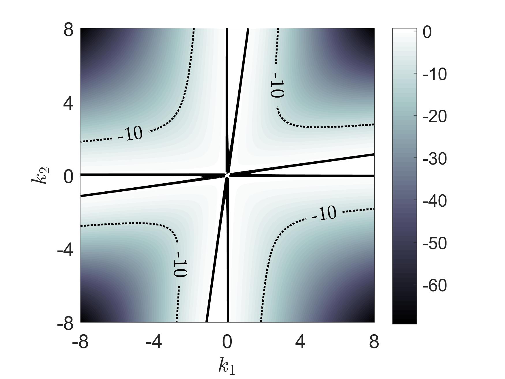
(a)

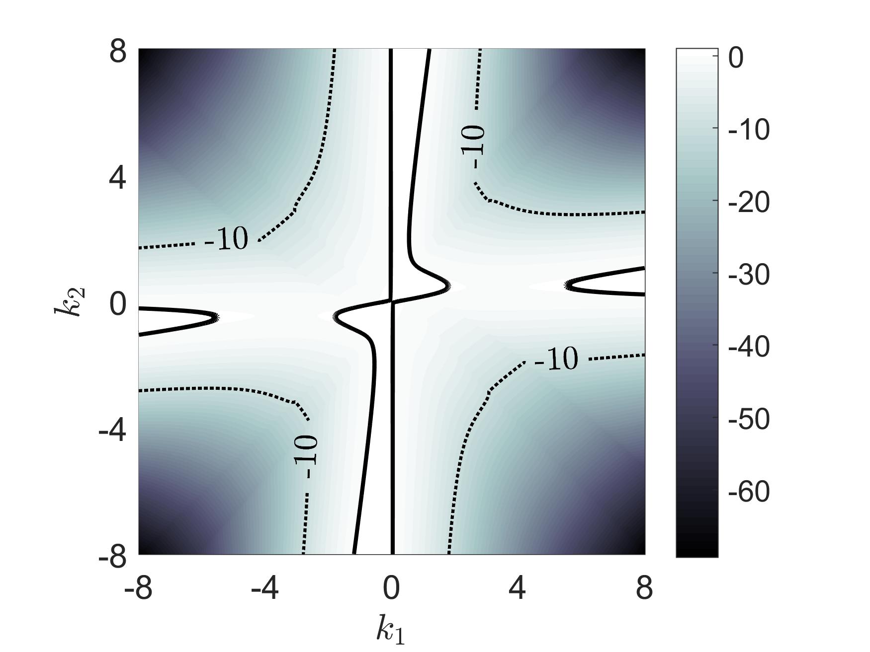
(b)

Figure 1: Stability diagram for (a) without and (b) with convection, for $\chi=0$, with $I=0.0001$, $\phi=0.5$, and $p^{(0)}=1$. Solid curves represent neutral stability.

These relations can be put in polar form, based on the polar representation

$$k=|\mathbf{k}|=\sqrt{k_{1}^{2}+k_{2}^{2}}\>\>\mbox{and}\>\>\vartheta=\mbox{tan}^{-1}(\kappa_{2}/\kappa_{1}).$$ (31)

where $k$ is the magnitude of the in-plane wave vector and $\vartheta$ is its angle with the direction of flow. With $c=\cos\vartheta$ and $s=\sin\vartheta$, the eigenvalue from (29) can be expressed as

$$\begin{split}&\lambda=\frac{1}{2\phi\tilde{\Phi}_{1}}\left[\beta\gamma k^{2}(c^{2}-s^{2})^{2}-2\tilde{\Phi}_{1}\Phi_{2}+2\phi c(s-\alpha c/\surd{2})+\tilde{\Phi}_{3}^{1/2}\right],\\ \mbox{where}\\ &\tilde{\Phi}_{3}=\Phi_{3}/k^{4}=\beta^{2}\gamma^{2}(c^{2}-s^{2})^{4}k^{4}-2\beta\gamma\phi c^{2}(c^{2}-s^{2})(\surd{2}\alpha-4cs)k^{2}\\ &+2\phi^{2}c^{2}(\alpha c-\surd{2}s)^{2}\>\mbox{and}\>\tilde{\Phi}_{1}=\Phi_{1}/k^{2}=1-\surd{2}\alpha cs,\end{split}$$ (32)

in which the trigonometric relations $c^{2}-s^{2}=\cos 2\vartheta$ and $2cs=\sin 2\vartheta$ also apply.

3.2 Transient Instability

Here, we consider the modifications of the stability analysis of Ref.​ 1 by the inclusion of convection and the vdW-CH gradient terms. Since that analysis is strictly valid only for the growth rates inferred from the initial state, the wave number $\mathbf{k}$ is to be interpreted here as its initial value $\boldsymbol{\kappa}$. We shall employ the term “ transient instability (or stability)” to denote positive (or negative) growth rates based on these initial values. The parameters employed in this study are the values proposed by Jop et al. (2005), namely $\mu_{0}=0.383$, $\mu_{\infty}=0.643$, and $I_{*}=0.279$, unless otherwise specified.

Some contours of the initial growth rate, represented by the real part of the eigenvalue $\lambda$ from (29), are shown in the stability diagram of Fig. 1, where (a) and (b) represent, respectively, stability with and without convection ($\mathbf{L}^{(0)}\equiv{\bf 0}$ in all terms except $I$ ), for $I=0.0001$ and $\chi=0$. The solid curves represent neutral stability $\lambda=0$, with lighter zones representing unstable regions. Fig. 1(a) is identical with the result of Ref.​ 1, whereas Fig. 1(b) shows that convection causes strong distortion of the neutral stability curve, eliminating parts of two unstable branches. Note that convection has a more pronounced effect in the regions of small $k$, as it represents a contribution of order zero in $k$ to (32), compared to terms of higher order in $k$ arising from the dissipative stresses.

Fig. 2 illustrates the effect of $\chi$, where it is obvious that the vdW-CH model provides a wave-number cut-off, shrinking unstable zones accordingly. By choosing very large $\chi$ one can, not surprisingly, eliminate almost completely the unstable zones.

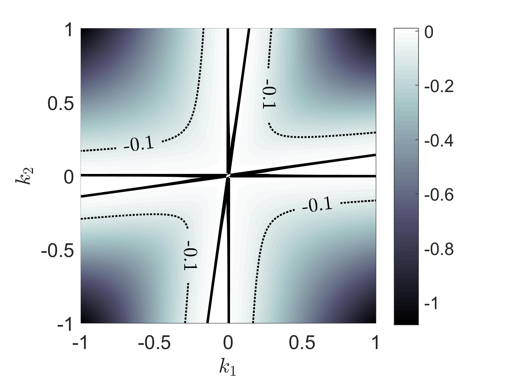
(a)

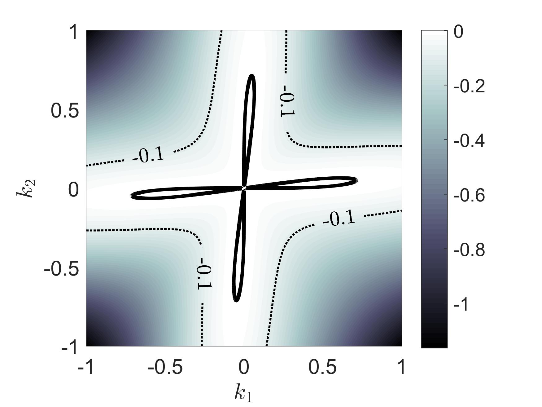
(b)

Figure 2: Stability without convection for (a) $\chi=0$ and (b) $\chi=0.005$, with $I=0.0001$, $\phi=0.5$, and $p^{(0)}=1$. Solid curves represent neutral stability.

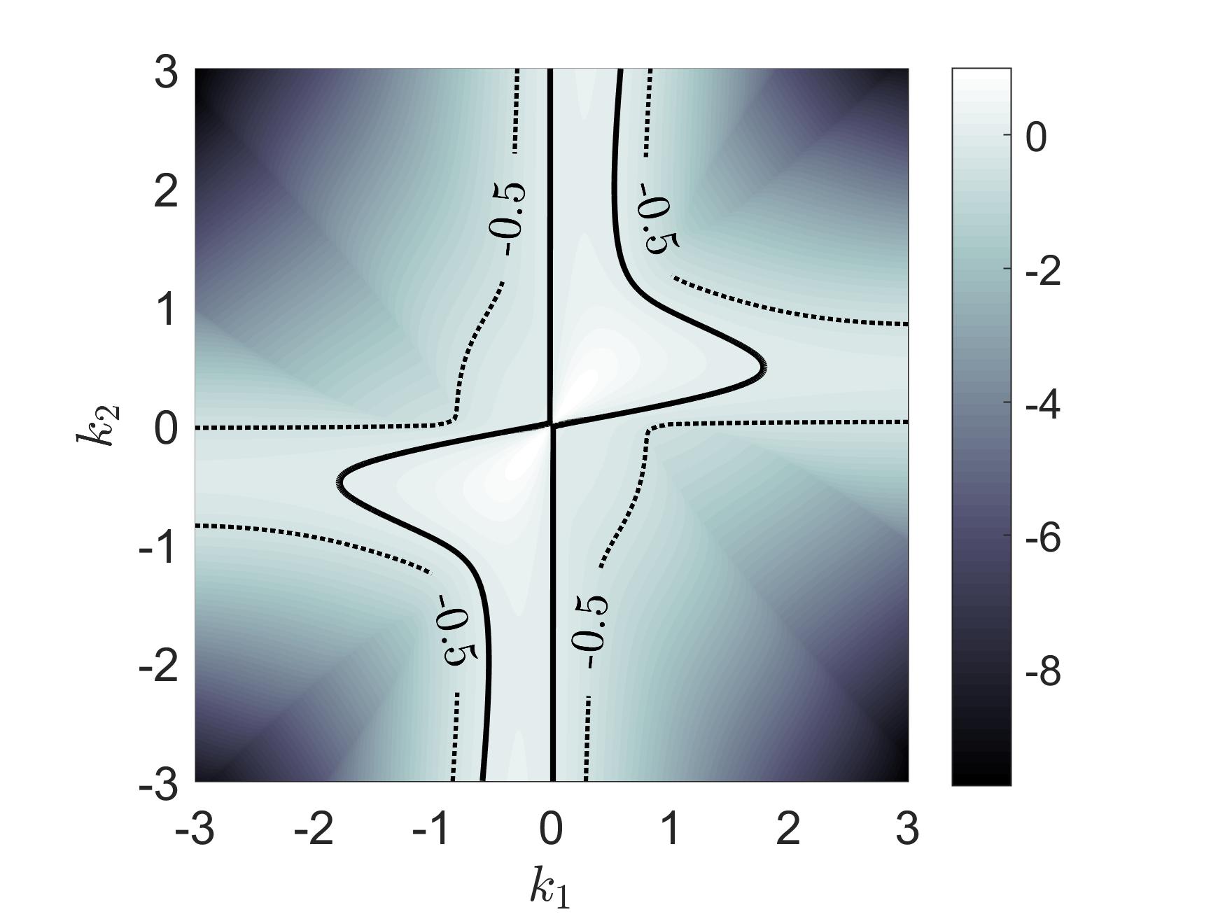
(a)

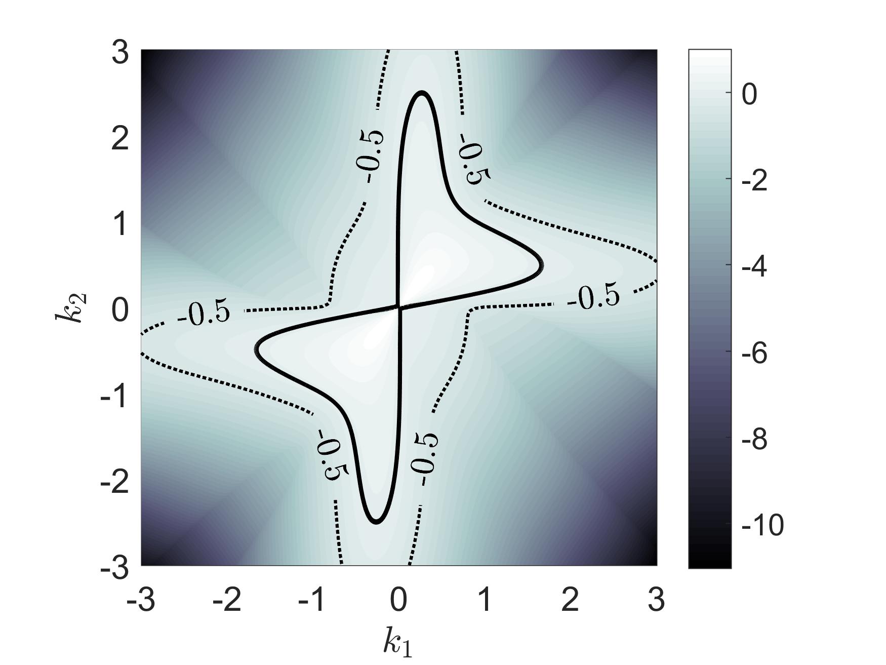
(b)

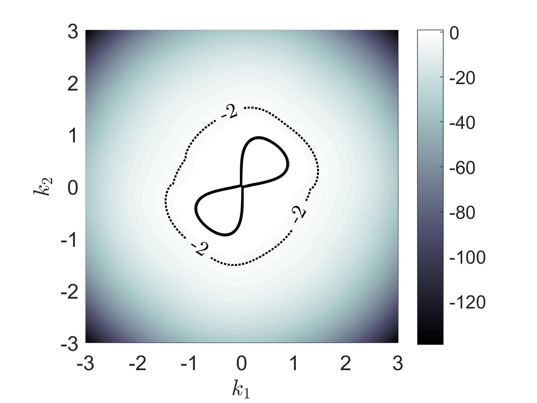
(c)

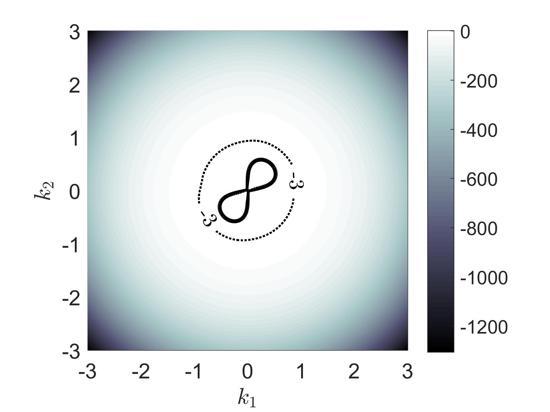
(d)

Figure 3: Stability with convection for increasing $\chi$ values: (a) $0$ (b) $0.001$ (c) $0.1$ and (d) $1$, with $I=0.0001$, $\phi=0.5$, and $p^{(0)}=1$.

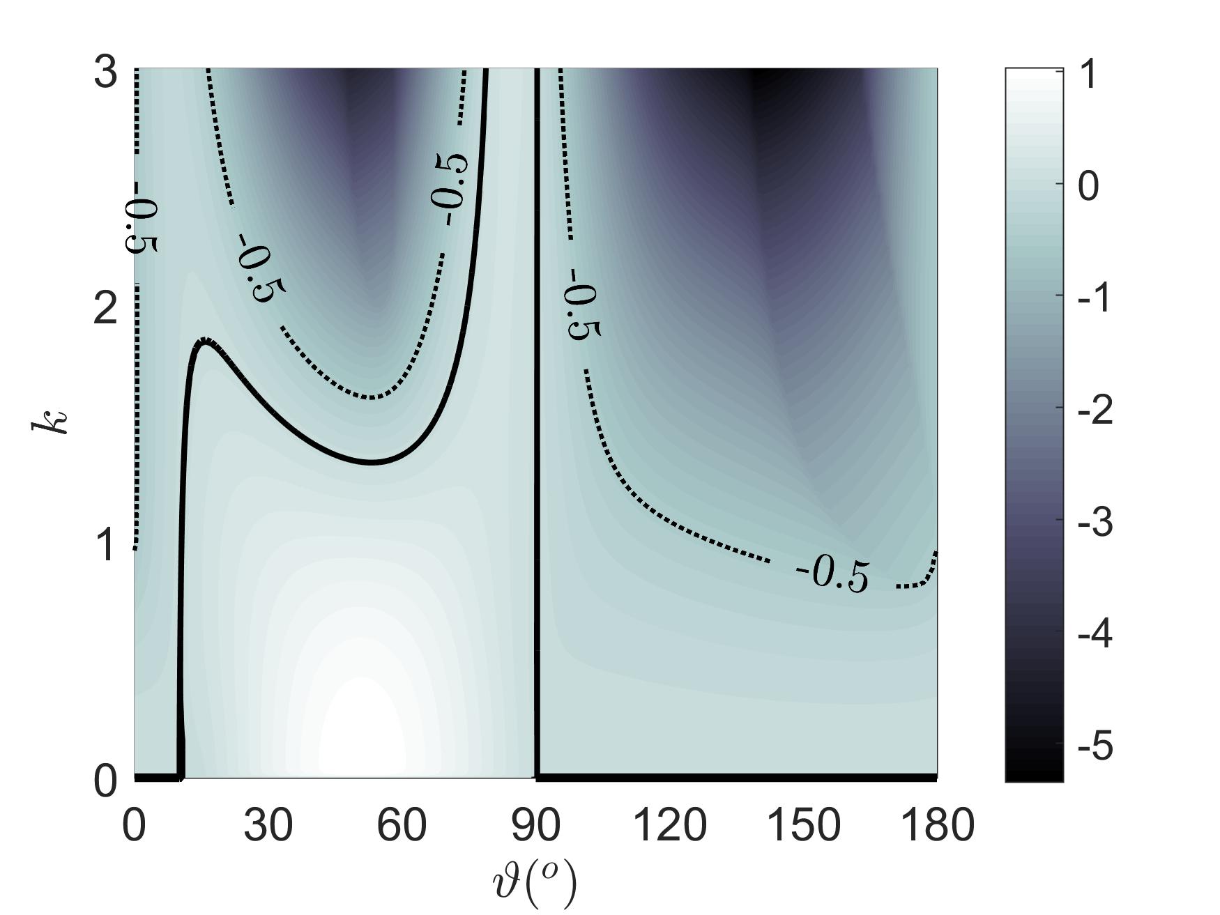
(a)

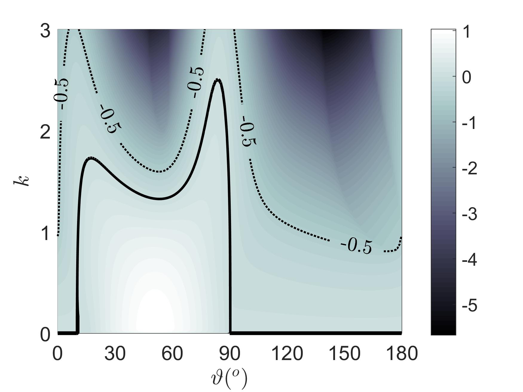
(b)

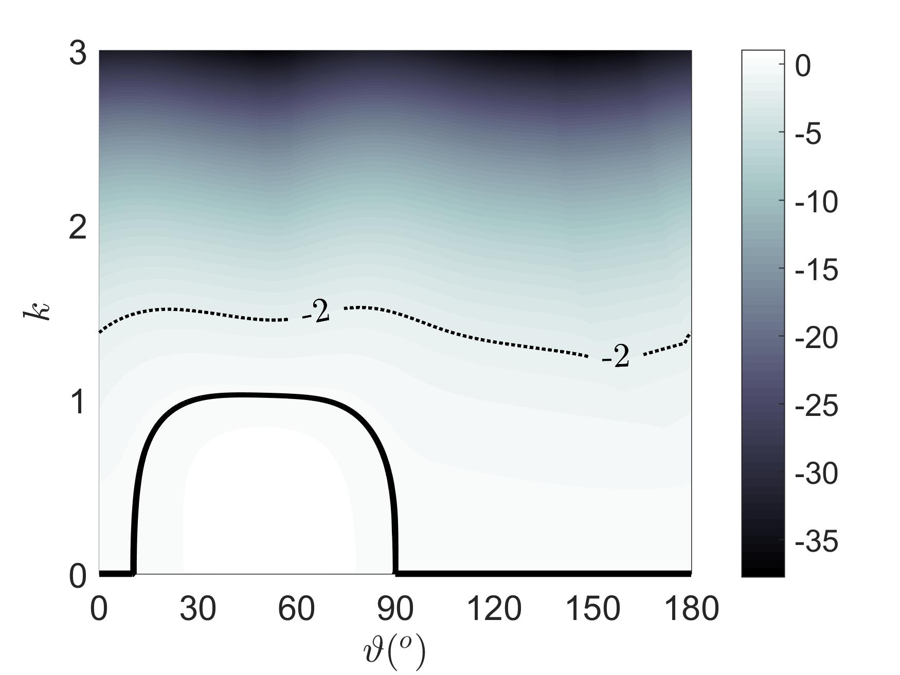
(c)

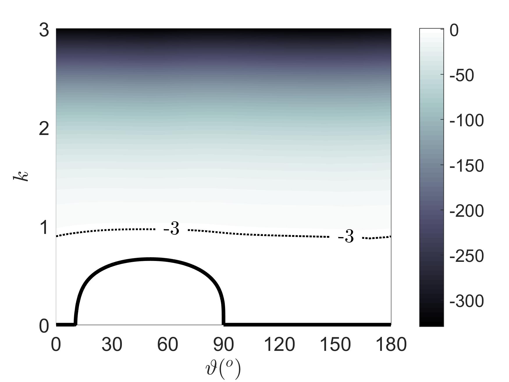
(d)

Figure 4: Fig. 3 in polar variables.

Fig. 3 shows the combined effects of convection and wave-number cut-off for various values of $\chi$, with $I=0.0001$. It is once again clear that the region of instability is greatly reduced by increasing $\chi$. This is perhaps made clearer by the plots in terms of polar variables in Fig. 4. Note that the growth rates in $0\leq\vartheta<\pi$ are also repeated in $\pi\leq\vartheta<2\pi$ when convection is included.

As discussed above, oscillatory behavior with $\mbox{Im}(\lambda)\neq 0$ arises for negative $\Phi_{3}$ and, writing $X=k^{2}>0$, we see from (32) that Re$(\lambda)$ and $\Phi_{3}$ are given by separate quadratic polynomials in $X$. Then, in order to have undamped oscillation, we must require the simultaneous conditions

$$\Phi_{3}<0\>\>\mbox{and}\>\>{\rm Re}(\lambda)\geq 0,\>\>\mbox{for}\>\>X>0,$$ (33)

on the these two quadratics. While we have not been able to provide a straight-forward and rigorous algebraic proof of the impossibility of (33), a detailed numerical investigation for various values of $k$ at closely spaced increments of $\vartheta$ in $(0,2\pi)$ and for various values of $\chi$ $I$ failed to achieve the condition. Hence, we are led to conjecture that oscillatory solutions are always damped.

Fig. 5 shows the corresponding imaginary part of the eigenvalue $\lambda$ for a particular set of parameter values, where finger-like regions bounded by the dashed lines contain the non-zero imaginary values of $\lambda$. Also shown are two contours of Re$(\lambda)$, the neutral stability curve and a curve representing damping. In line with the above conjecture, the oscillatory behavior is damped.

Following Ref.​ 1, we present in Fig. 6 a stability diagram in the $I$-$\Delta\mu$ plane to show the effect of $\chi$ with and without convection, for $\mathbf{k}=(0.1,0.8)$ (or $k=0.806,\>\>\vartheta=82.9^{\circ})$. The curves shown there are loci of neutral stability and regions inside the closed curves or beneath the open curves are the stable regions. The curve $\chi=0$ in Fig. 6(a) is a magnified version of that given in Ref.​ 1, indicating that the perfectly-plastic case of constant $\mu$, with $\Delta\mu=0$ is always unstable. However, this instability is apparently removed at a critical $\chi$ value between 0.001 and 0.002, where the closed curve opens up to form an unbounded stable region. Interestingly, this critical $\chi$ value is nearly ten times larger when convection is included, as illustrated by Fig. 6(b).

In summary, the preceding results indicate that convection distorts the regions of transient instability, completely eliminating instability for some directions of $\mathbf{k}$ while leading to short wavelength instability for others, in the absence of cut-off by the gradient terms in $\chi$.

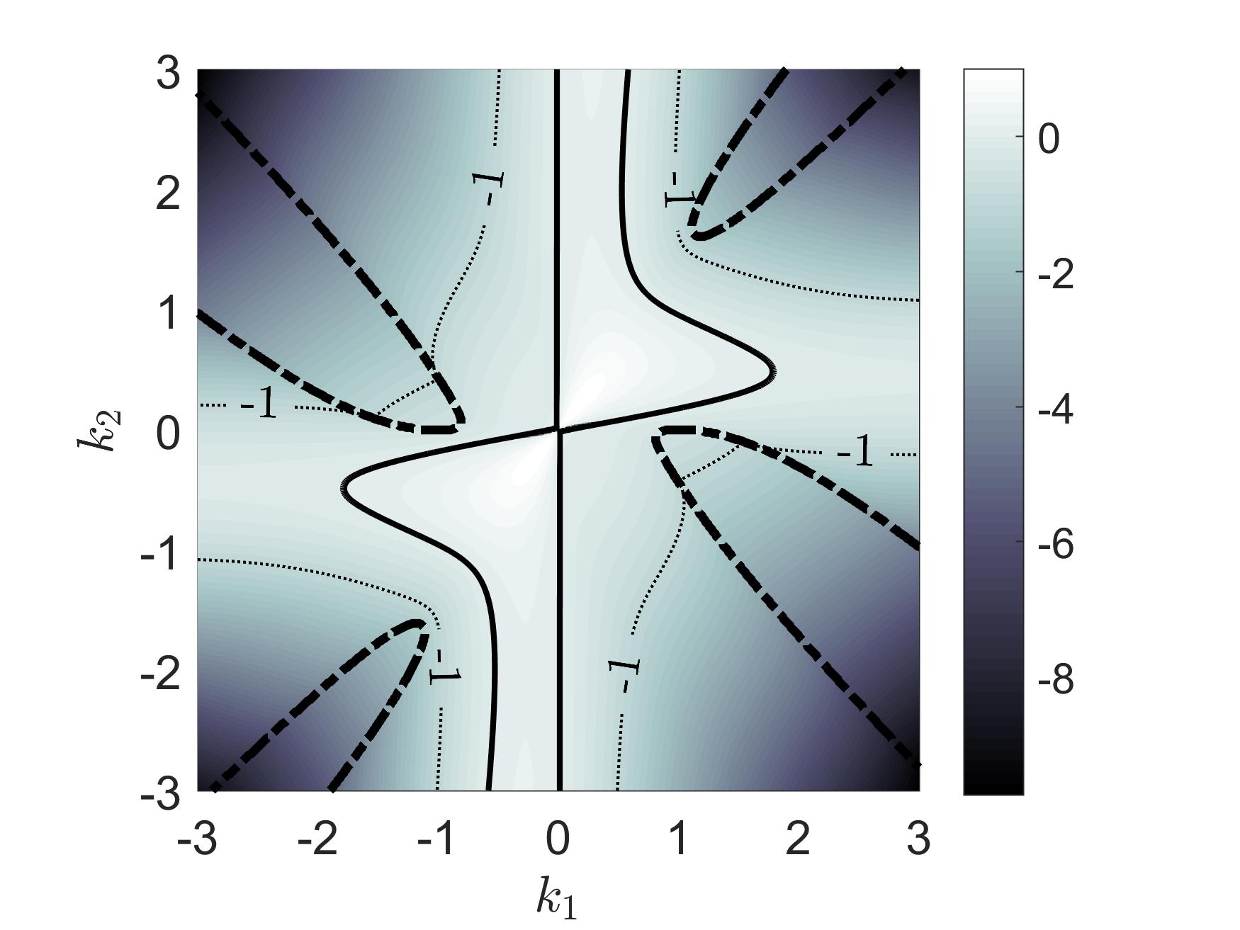
Figure 5: Oscillatory behavior resulting from convection, for $\chi=0$, $I=0.0001$, $p^{(0)}=1$, and $\phi=0.5$. The oscillation frequency is non-zero within finger-like regions bounded by dashed curves and equal to zero upon and outside these curves. The solid and dotted curves are contours of the real part of $\lambda$, the former representing neutral stability.

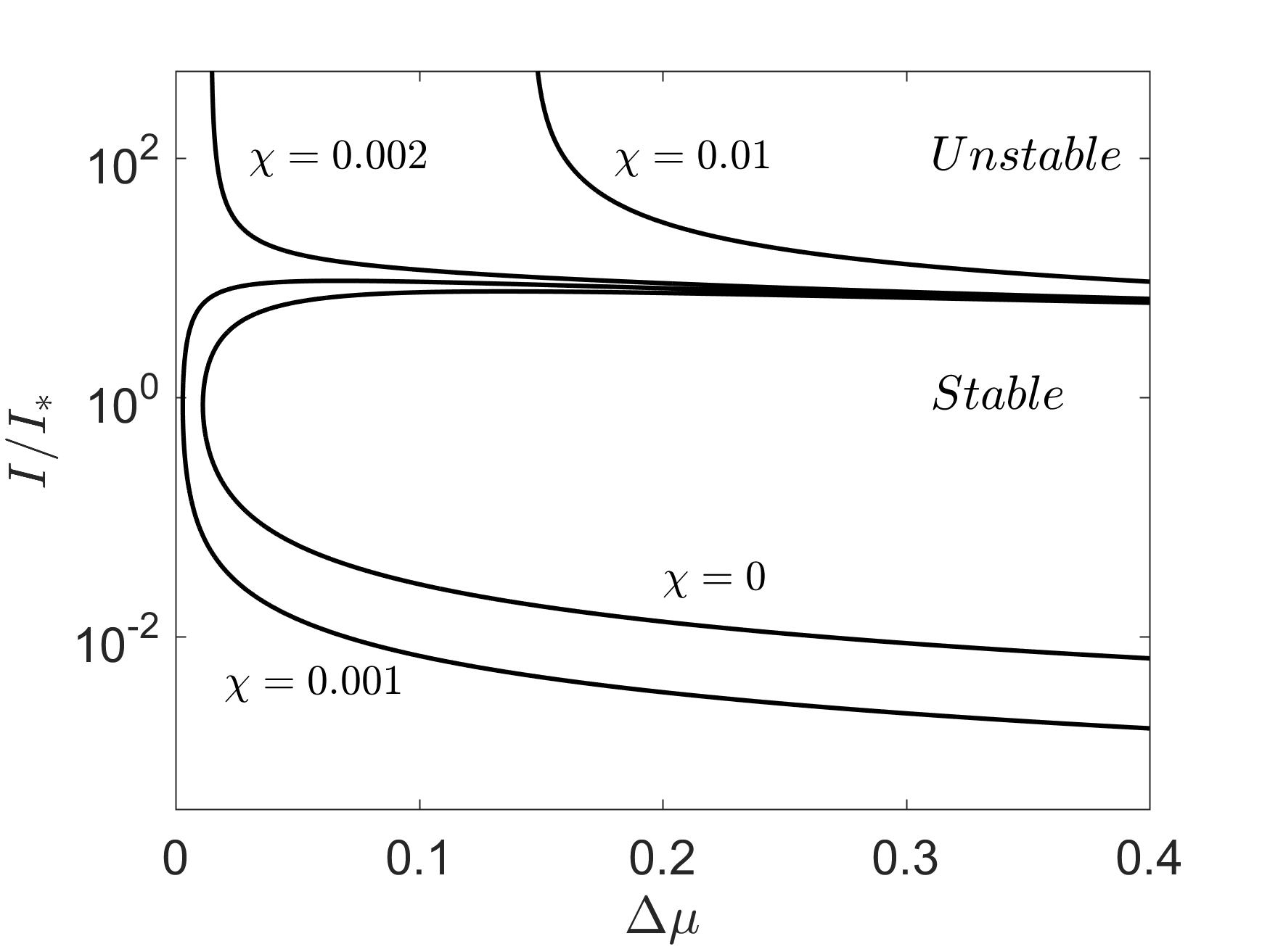
(a)

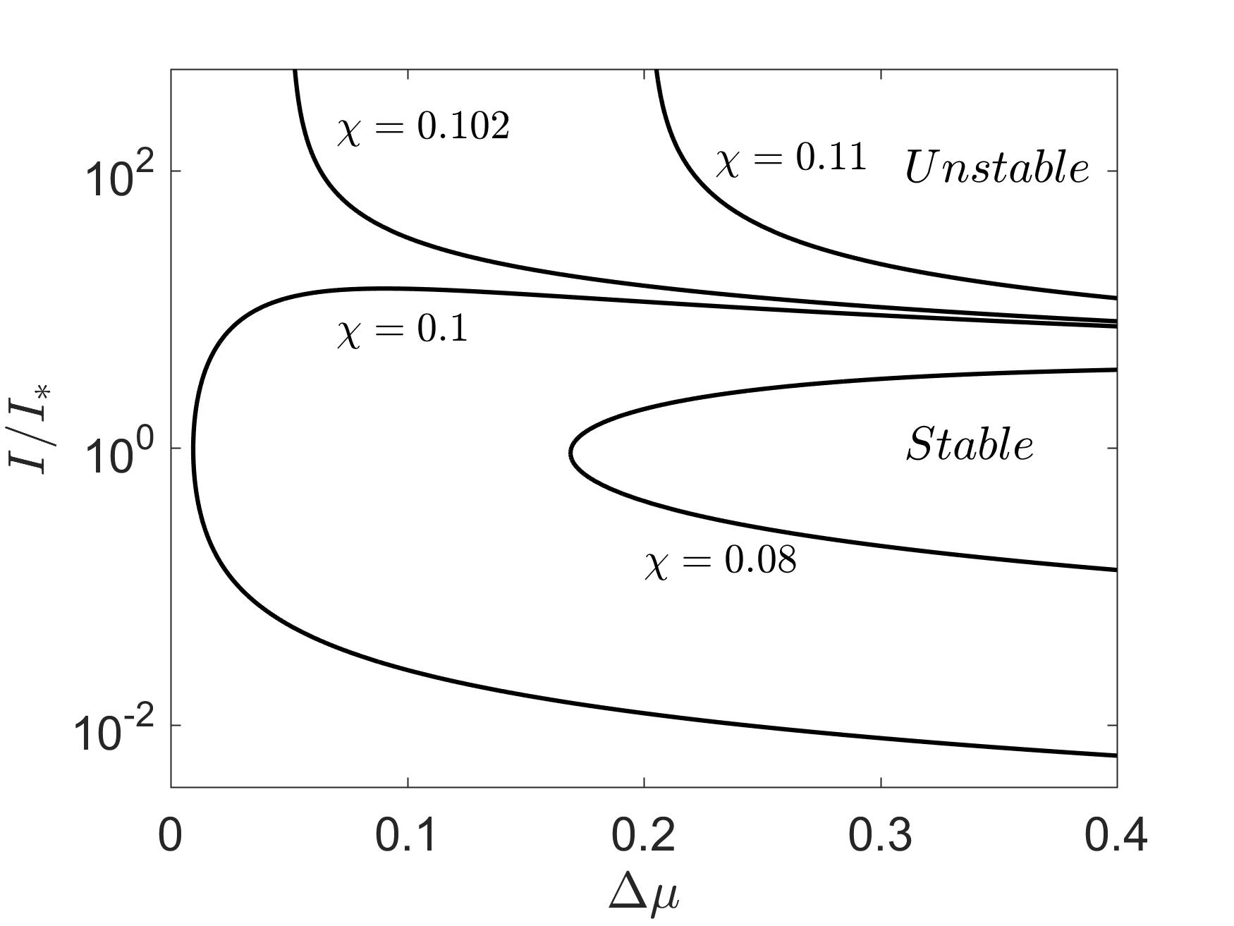
(b)

Figure 6: Stability in the $I$-$\Delta\mu$ plane, (a) without and (b) with convection, showing the effect of $\chi$, where $\mathbf{k}=(0.1,0.8)$ ($k=0.806,\>\>\vartheta=82.9^{\circ}$ ), $p^{(0)}=1$, and $\phi=0.5$.

3.3 Asymptotic behavior

According to (26), for large $t$ and $\kappa_{1}\neq 0$ we have $|k_{2}|>>|k_{1}|$, resulting in the following asymptotic forms:

$$\begin{split}&A_{11}\sim k_{2}^{2}[(\beta-1)\gamma-2\chi k_{2}^{2}]/\phi,\>\>A_{12}\sim-A_{12}\sim\beta\gamma k_{1}k_{2}/\phi,\\ &A_{22}\sim-k_{2}^{2}[\gamma+2\chi k_{2}^{2}]/\phi,\>\>\mbox{and}\>\>\lambda\sim A_{11},\end{split}$$ (34)

up to terms of relative magnitude $O(|k_{2}|^{-1})$ . Since $\beta\!-\!1=\!-\!\stackrel{{\scriptstyle\>\prime}}{{\mu}}\>\>\leq 0$, for $\mu_{\infty}\geq\mu_{0},$ it follows from (34) that the local growth rate for $\chi\geq 0$ is never positive for large $t$ whenever $\kappa_{1}\neq 0$. In the exceptional case $\kappa_{1}=0$, where $\mathbf{k}(t)\equiv\boldsymbol{\kappa}=(0,\kappa_{2})$, it is easy to show by means of (28) -(29) that $\lambda$ is never positive for $\chi\geq 0$. Therefore, we conclude that any transient instability is eventually killed off by wave vector stretching, irrespective of vdW-CH regularization. The resulting asymptotic stability is illustrated by a numerical solution of (23). For the incompressible planar flows considered here, this is facilitated by the following closed-form solution for the stream function.

3.3.1 Scalar solution to (23)

For planar flow, the condition of incompressibility can be expressed in the usual way in terms of a stream function $\uppsi(x_{1},x_{2})$ as

$$v_{1}=\partial_{x_{2}}\uppsi,\>\>v_{2}=-\partial_{x_{1}}\uppsi$$ (35)

which in terms of Fourier transforms become

$$\begin{split}&\hat{v}_{1}=\imath k_{2}\hat{\uppsi},\>\>\hat{v}_{2}=-\imath k_{1}\hat{\uppsi},\>\>\mbox{or}\>\>\hat{\mathbf{v}}=\imath\mathbf{k}^{\bot}\hat{\uppsi},\\ &\mbox{where}\>\>\mathbf{k}^{\bot}=(k_{2},-k_{1})={\bf Q}\mathbf{k},\>\>{\bf Q}=\left[\begin{array}[]{rr}0&1\\ -1&0\end{array}\right],\end{split}$$ (36)

${\bf Q}$ is orthogonal, and $\mathbf{k}^{\bot}$ is identical with the flipped wave vector introduced in Ref.​ 1. It is easy to see that the preceding linear relations also apply to perturbations. Hence, after making use of $\mathop{}\mathrm{d}\mathbf{k}/\!\!\mathop{}\mathrm{d}t=-{\mathbf{L}}^{(0)T}\mathbf{k}$ the ODE can be reduced to the form

$$\mathbf{k}\frac{\mathop{}\mathrm{d}\hat{\uppsi}}{\mathop{}\mathrm{d}t}={\bf B}\mathbf{k}\hat{\uppsi},\>\>\mbox{where}\>\>{\bf B}={\bf Q}^{T}\mathbf{A}{\bf Q}+\mathbf{L}^{(0)T}$$ (37)

Now, $\mathbf{k}$ and $\mathbf{k}^{\bot}$ serve as orthogonal basis for 2D vectors and it is easy to show that $\mathbf{k}^{\bot}\!\cdot\!{\bf B}\mathbf{k}=0$, i.e. the right hand side of (37) has zero component in direction $\mathbf{k}^{\bot}$. By Fredholm’s theorem, applied implicitly in Ref.​ 1, this establishes that $\mathbf{k}$ is in the range of ${\bf B}$ and, hence, is an eigenvector of ${\bf B}$. Thus, (37) involves only components in direction $\mathbf{k}$, given by orthogonal projection as:

$$\frac{\mathop{}\mathrm{d}\hat{\uppsi}}{\mathop{}\mathrm{d}t}=\Lambda(t,\boldsymbol{\kappa})\hat{\uppsi},\>\>\mbox{where}\>\>\Lambda=\frac{\mathbf{k}\!\cdot\!{\bf B}\mathbf{k}}{k^{2}},$$ (38)

where

$$\Lambda=\frac{1}{\phi k^{2}\Phi_{1}}\left\{\phi\left[(k_{1}k_{2}(k^{2}+\Phi_{1})-\surd{2}\>\alpha k_{1}^{4}\right]+\beta\gamma k^{2}(k_{1}^{2}-k_{2}^{2})^{2}-\Phi_{1}\Phi_{2}k^{2}\right\}$$ (39)

is the eigenvalue for eigenvector $\mathbf{k}$ of ${\bf B}$ .

It follows that the solution to the linear stability problem for constant $\mathbf{L}^{(0)}$ is given by

$$\hat{\mathbf{v}}^{(1)}=\hat{\uppsi}_{0}{\bf Q}\exp\left\{\int_{0}^{t}\Lambda(t^{\prime},\boldsymbol{\kappa})\mathop{}\mathrm{d}t^{\prime}\right\}\mathbf{k}=\hat{\uppsi}_{0}{\bf Q}\exp\left\{\mathbf{I}\!\int_{0}^{t}\Lambda(t^{\prime},\boldsymbol{\kappa})\mathop{}\mathrm{d}t^{\prime}-\mathbf{L}^{(0)T}t\right\}\boldsymbol{\kappa},$$ (40)

which gives

$$|\hat{\mathbf{v}}^{(1)}|=|\hat{\uppsi}_{0}|k\exp\left\{\int_{0}^{t}\Lambda(t^{\prime},\boldsymbol{\kappa})\mathop{}\mathrm{d}t^{\prime}\right\},$$ (41)

where, in all the above formulae,

$$\mathbf{k}(t,\boldsymbol{\kappa})=\exp\left\{-\mathbf{L}^{(0)T}t\right\}\boldsymbol{\kappa},\>\>\mbox{with}\>\>k=\left[\boldsymbol{\kappa}\!\cdot\!\exp\left\{-\mathbf{L}^{(0)}t\right\}\exp\left\{-\mathbf{L}^{(0)T}t\right\}\boldsymbol{\kappa}\right]^{1/2}$$ (42)

It is easy to show that (41) gives the same result as that obtained by substitution of $\hat{\mathbf{v}}^{(1)}=\uppsi\mathbf{k}^{\bot}$ into (24). Moreover, when convection is neglected one finds that $\mathbf{k}\!\cdot\!{\bf B}\mathbf{k}=\mathbf{k}^{\bot}\!\cdot\!\mathbf{A}\mathbf{k}^{\bot}$, and, hence, that $\mathbf{k}^{\bot}$ is an eigenvector of $\mathbf{A}$ with eigenvalue $\Lambda$, as already found in Ref.​ 1.

Making use of the asymptotic form (34), we find for large $k$ with $|k_{2}|>>|k_{1}|$ that

$$\Lambda\sim\frac{k_{2}^{2}}{\phi\tilde{\Phi}_{1}}[(\beta-\tilde{\Phi}_{1})\gamma-2\tilde{\Phi}_{1}\chi k_{2}^{2}]\sim\lambda,\>\>\mbox{with}\>\>\tilde{\Phi}_{1}=\Phi_{1}/k^{2}\sim\Phi_{1}/k_{2}^{2},\>\>\mbox{for}\>\>t\rightarrow\infty,\>\>$$ (43)

where $\lambda$ is the eigenvalue of $\mathbf{A}$ with largest real part, which confirms the asymptotic behavior inferred previously from (34).

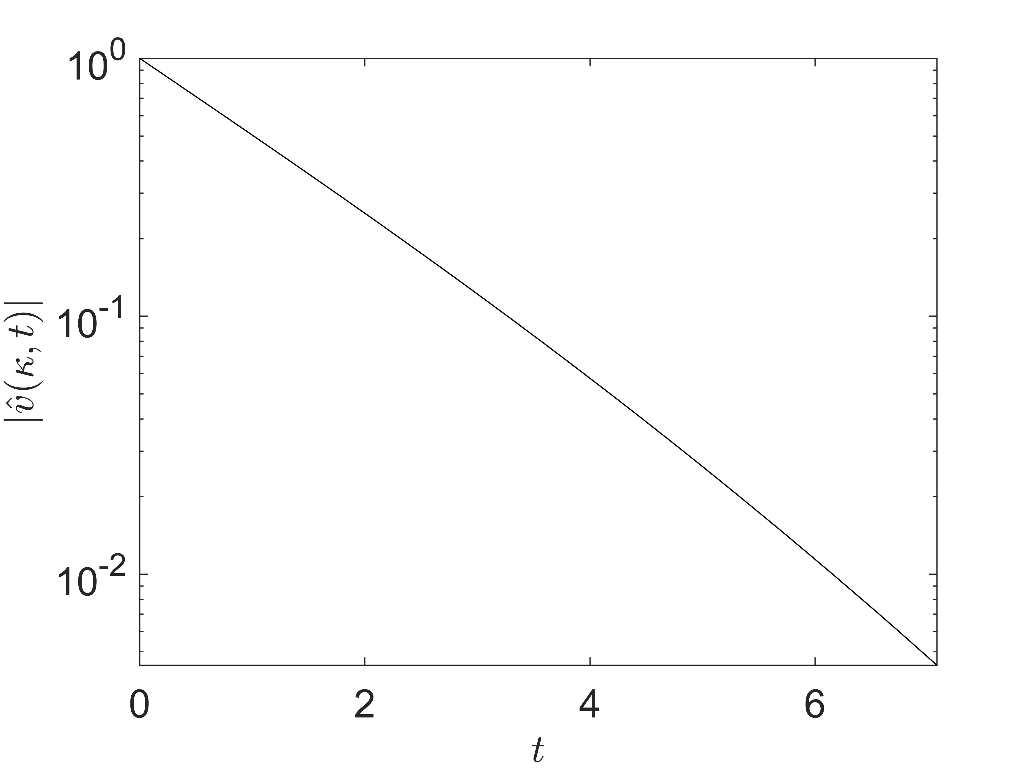
(a)

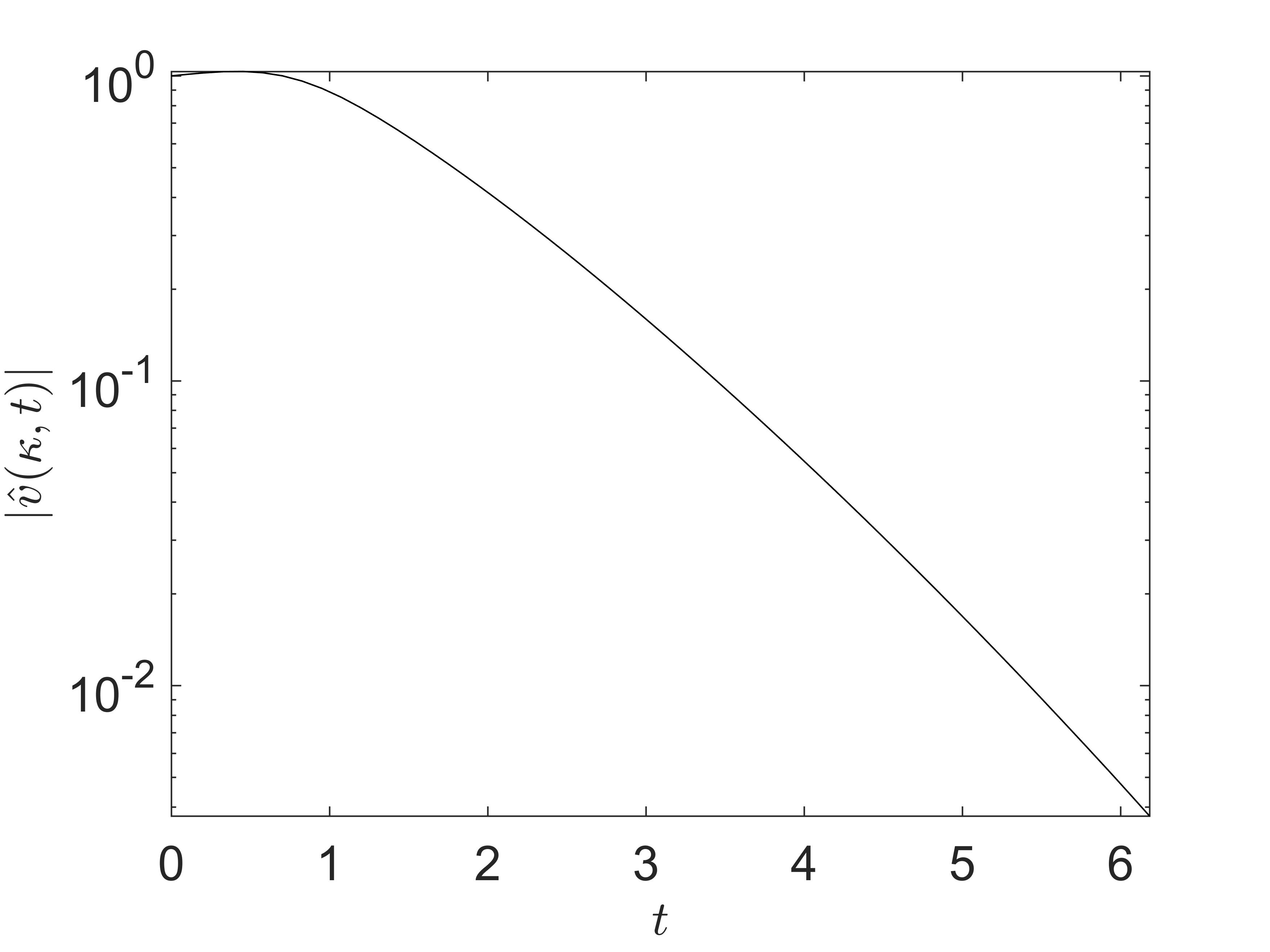
(b)

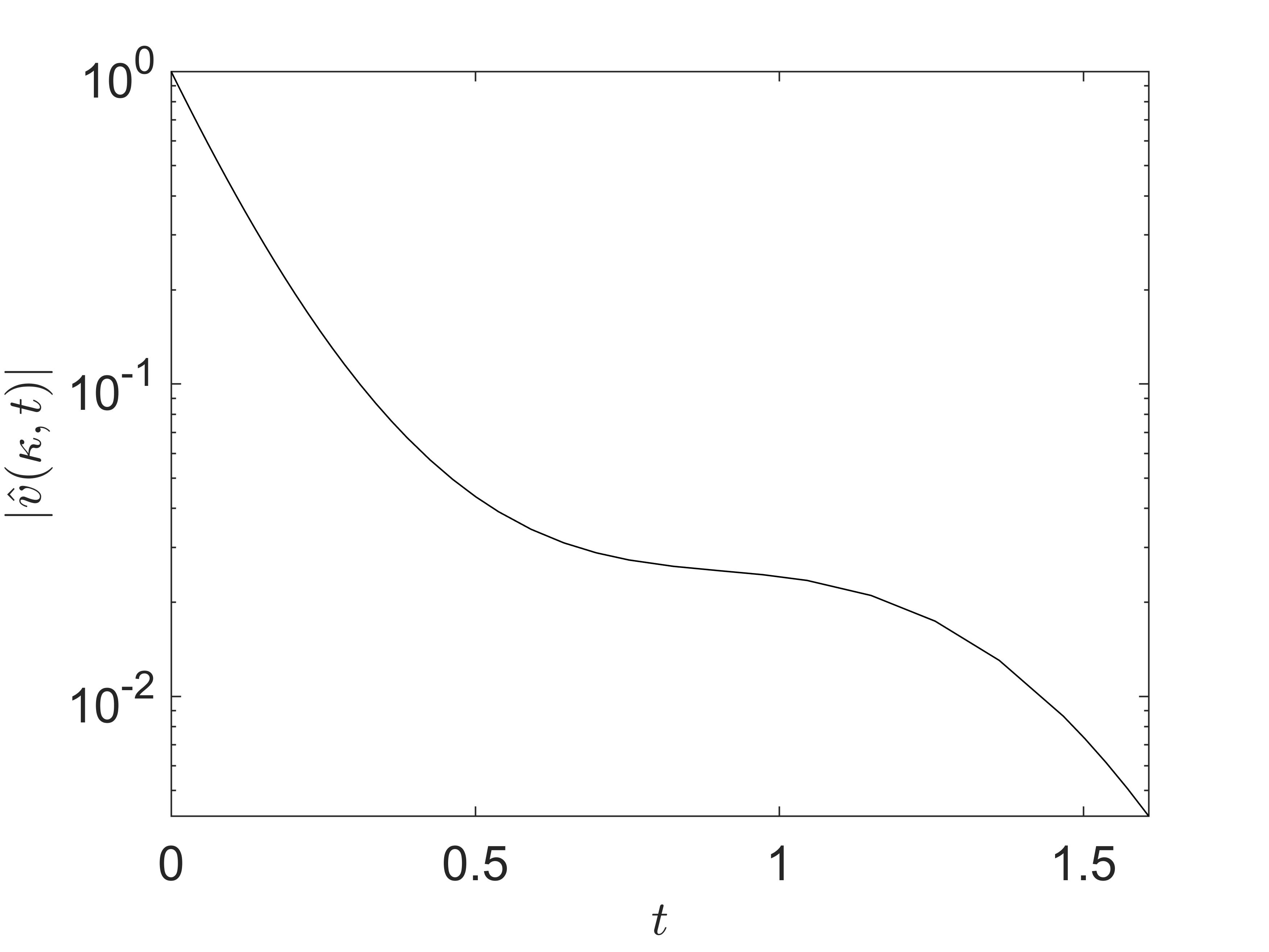
(c)

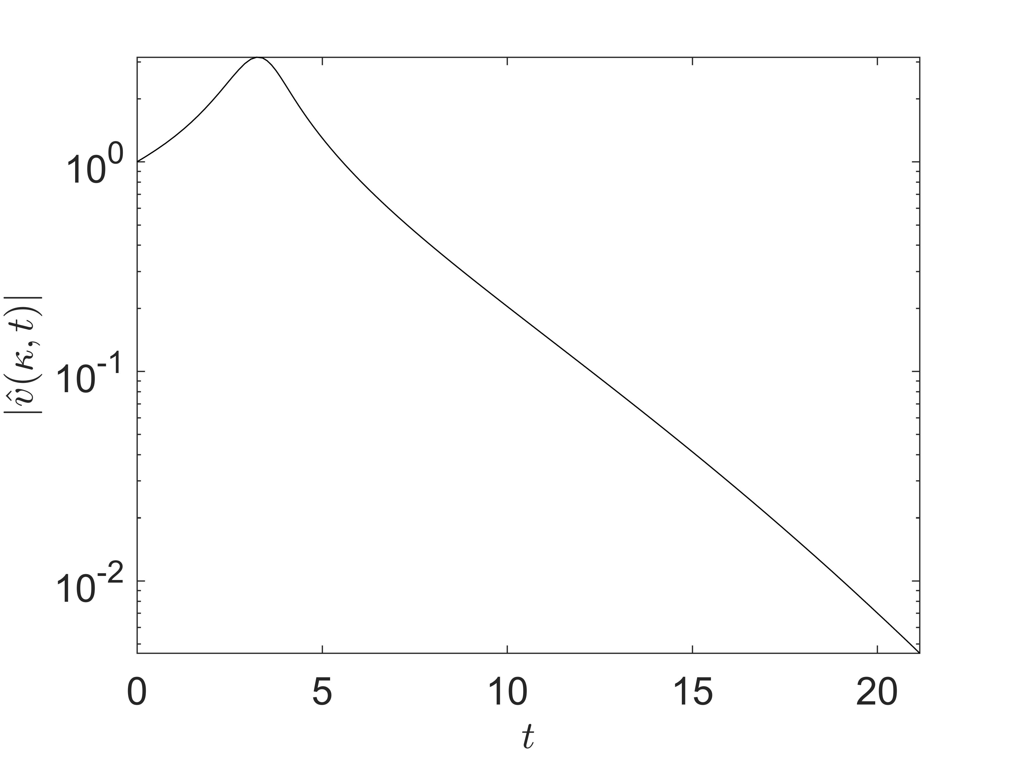
(d)

Figure 7: Magnitude $|\hat{\boldsymbol{\upsilon}}(\boldsymbol{\kappa},t)|$ of various Fourier modes vs. $t$ for $\chi=10^{-6}$ and initial conditions (a) $\boldsymbol{\kappa}=(-.5,0.866)$; (b) $\boldsymbol{\kappa}=(-0.707,-0.707)$; (c) $\boldsymbol{\kappa}=(-3.54,-3.54)$; (d) $\boldsymbol{\kappa}=(0.259,0.966)$.

Fig. 7 presents semi-log plots of (41), with $|\hat{\uppsi}_{0}|=1/\kappa$ and, hence, $|\hat{\mathbf{v}}^{(1)}|=1$ at $t=0$, as obtained from the integration of (38) by means of the the finite difference approximation (FDA) and the MATLAB^®  numerical integrator “ode45” for two values $\kappa=1$ and $\kappa=5$ and parameter values

$$I^{(0)}=0.001,\>\>I_{*}=0.2790,\>\>\mu_{0}=0.3830,\>\>\mu_{\infty}=0.6430,\phi=0.5,\>\>p^{(0)}=1,$$

with cessation of integration for values of $|\hat{\boldsymbol{\upsilon}}|$ less than 0.001. Figs. 7(b) and 7(c) serve to illustrate the effect of $\kappa=|\boldsymbol{\kappa}|$ for $\vartheta=45^{\circ}$. These figures are not changed drastically by taking $\chi=1$, whereas the transient instability in Fig. 7(d) is completely eliminated.

As pointed out above in the paragraph following (19), material instability can also be characterized as the loss of generalized ellipticity in the quasi-static (inertialess) field equations. The latter can be obtained by omitting all inertia terms from (23) and (37), which gives the following expression for $\Lambda$

$$\Lambda=\frac{\beta\gamma(k_{1}^{2}-k_{2}^{2})^{2}}{\Phi_{1}(\mathbf{k})}-(\gamma k^{2}+2\chi k^{4})=-\frac{\beta\gamma(\xi_{1}^{2}-\xi_{2}^{2})^{2}}{\Phi_{1}(\boldsymbol{\xi})}+\gamma\xi^{2}-2\chi\xi^{4},$$ (44)

where $\boldsymbol{\xi}=\imath\mathbf{k}$, the so-called symbol, is the algebraic representation of the differential operator $\nabla$ (Renardy & Rogers, 2006). Hence, the positive definite quadratic form $\Phi_{1}(\boldsymbol{\xi})$ in real-valued $\boldsymbol{\xi}$ represents an anisotropic Laplacian. The latter can be reduced to the usual Laplacian on an appropriate coordinate system, with $\Phi_{1}^{-1}$ representing the corresponding Green’s function.

Now, generalized ellipticity may be defined as the requirement that the differential operator represented by $-\Lambda$ be positive definite in real-valued $\xi$ (Browder, 1961; Brezis & Browder, 1998; Renardy & Rogers, 2006), which in the present context requires that $\chi>0$. Therefore, the vdW-CH regularization is essential for material stability according to this criterion, and it seems worthwhile to illustrate how this regularization might serve to impart a diffuse length scale to shear bands.

4 Model of a steady shear band and its non-linear stability

Based on the preceding analysis, with large $k_{2}$ representing dominant gradients in the direction $y=x_{2}$, we assume a single stabilized shear band localized at $y=0$ in an initially unperturbed shear flow with ${\bf g}=0,\>\>\nabla p=0,$ and $\mathbf{v}=(y,0)$ will take the form of a stable, fully-developed flow in the $x=x_{1}$ direction with $\mathbf{v}=(u(y),0)$ and with the partial derivatives $(\partial_{t},\partial_{x})$ of all quantities vanishing. Hence, after one integration with respect to $y$ the momentum balance (11) reduces to the ODE

$$\begin{split}u^{\prime\prime\prime}&=f(u^{\prime})=\frac{\mu(I)-\mu(I^{(0)})}{2\surd{2}\>\chi\>I^{(0)2}}{\rm sgn}(u^{\prime})\\ &=\frac{(\mu_{\infty}-\mu_{0})I_{*}(|u^{\prime}|-1){\rm sgn}(u^{\prime})}{2\surd{2}\>\chi\>I^{(0)}(I^{(0)}+I_{*})(I^{(0)}|u^{\prime}|+I_{*})},\\ &\mbox{with}\>\>I=I^{(0)}|u^{\prime}|\>\>\mbox{and}\>\>I^{(0)}=1/\surd{p},\end{split}$$ (45)

where primes denote differentiation with respect to $y$ and we employ the non-dimensional variables (18). We further invoke the condition $u^{\prime}\rightarrow 1$ for $|y|\rightarrow\infty$, corresponding to the unperturbed flow. Hence, assuming that $u(y)$ is an odd function of $y$ we may focus on the half space $y>0$ with further conditions $u(0)=0$.

As discussed below, the form of the ODE (45) indicates that the limit $\chi\rightarrow 0$ leads to a well-known singular perturbation for small $\chi$, in which that one may generally neglect the vdW-CH terms in the “outer region” lying outside a thin shear band of thickness $O(\chi^{1/2})$, which we recall represents the ratio of microscopic to macroscopic length scales.

To pursue an analytical treatment, we note that the function $f(u^{\prime})$ in (45) can be written as derivative $\mathop{}\mathrm{d}\tilde{\psi}_{0}/\mathop{}\mathrm{d}u^{\prime}$ of a modified form of the dissipation potential $\psi_{0}$:

$$\tilde{\psi}_{0}(u^{\prime})=\frac{(\mu_{\infty}-\mu_{0})I_{*}}{2\surd{2}\chi I^{(0)3}}\left[\frac{|u^{\prime}|}{1+I_{*}/I^{(0)}}-\ln\left(\frac{I^{(0)}|u^{\prime}|}{I_{*}}+1\right)\right].$$ (46)

Then, by a standard method, (45) can be integrated twice to yield $u^{\prime}$ as implicit function of $y$:

$$y=Y(u^{\prime},u^{\prime}_{0})=\int_{u^{\prime}}^{u^{\prime}_{0}}\frac{\mathop{}\mathrm{d}w}{\sqrt{2[\tilde{\psi}_{0}(w)-\tilde{\psi}_{0}(1)]}}.$$ (47)

Note that (45)-(46) imply that $\tilde{\psi}_{0}(w)-\tilde{\psi}_{0}(1)\rightarrow 0$ quadratically and $y\rightarrow\infty$ logarithmically in $|w\!-\!1|$ as $w\rightarrow 1$.

It is an easy matter to convert the preceding relation to the second implicit form

$$\begin{split}&u=y+\int_{u^{\prime}}^{u^{\prime}_{0}}\frac{(w-1)\mathop{}\mathrm{d}w}{\sqrt{2[\tilde{\psi}_{0}(w)-\tilde{\psi}_{0}(1)]}}\sim y+\Delta_{0},\>\>\mbox{for}\>\>|u^{\prime}|\rightarrow 1,\\ &\mbox{where}\>\>\Delta_{0}=\int_{1}^{u^{\prime}_{0}}\frac{(w-1)\mathop{}\mathrm{d}w}{\sqrt{2[\tilde{\psi}_{0}(w)-\tilde{\psi}_{0}(1)]}},\end{split}$$ (48)

which gives $u^{\prime}$ implicitly as function of $u$ and $y$ and shows that $u^{\prime}_{0}=u^{\prime}(0)$ is a free parameter that must be specified to complete the solution. The quantity $\Delta_{0}$, the intercept at $y=0$ of the asymptotic solution for $y\rightarrow\infty$, represents one-half the apparent slip on a shear band of zero thickness at $y=0$ as seen in the far field. It can be calculated by numerical quadrature for given $u^{\prime}_{0}$ and provides a quite useful criterion for convergence of the numerical solution considered next. The quadrature was performed in the present study by means of the  MATLAB^®  function ”integral.m”.

Note that under the rescaling

$$\bar{y}=y/I^{(0)}\surd{\chi},\>\>\bar{u}=u/I^{(0)}\surd{\chi},\>\>\bar{\psi}=I^{(0)2}\chi\tilde{\psi}_{0},\>\>\bar{\Delta}_{0}=\Delta_{0}/I^{(0)}\surd{\chi},$$ (49)

(where overbars are not to be confused with prior usage to denote the present non-dimensional variables) $u^{\prime}$ is invariant and the relation (48) gives, upon division by $I^{(0)}\surd{\chi}$ , a description of the inner layer discussed above in terms of $\bar{y}$, $\bar{u}$, $\bar{\psi}$, and $\bar{\Delta}_{0}$.

Since numerical methods are generally necessary to treat (47) or (48), it is more efficacious to integrate (45) numerically. Upon replacement of $u$ and $y$ by the scaled variables $\bar{u}$ and $\bar{y}$ defined in (49), the ODE (45) maintains the same form, with

$$\chi\rightarrow 1,\>\>I^{(0)}\rightarrow 1,\>\>I_{*}\rightarrow I_{*}/I^{(0)}\>\>$$ (50)

Moreover, one can show that the replacement of $\chi$ by $\chi\mu_{0}$ in (49), converts the parameter $\Delta\mu=\mu_{\infty}\!-\!\mu_{0}$ to $\Delta\mu/\mu_{0}$, with $\mu_{0}\rightarrow 1$ elsewhere. Since the same transformation applies to the full momentum balance, it serves to justify the general validity of the stability plot of Barker et al. (2015) represented by Fig. 6 in the present paper. We do not adopt this additional scaling in the present paper, since $\mu_{0}$ is not varied.

As pointed out above, the quantity $u^{\prime}_{0}=u^{\prime}(0)$ is an unknown that must in principle be specified by the complete solution to the full momentum balance. We recall that such a numerical solution was carried out in Ref.​ 1 for a non-homogeneous shear flow for $\chi=0$ . While the authors found instability, it is not clear what role non-linear effects may play and, in line with comments in the Introduction, whether their numerics serve to rule out asymptotically stable states with sharp shear bands.

To pursue numerical solutions of the full momentum balance would take us well beyond the scope of the present work . Instead, we provide below a one-dimensional analysis of the non-linear stability of steady shear bands against normal sinusoidal perturbations as a function of $u^{\prime}(0)$. For illustrative purposes, we consider here the assumption that, up to factors of order unity, $u^{\prime}(0)\sim k_{2,\rm{max}}$, where $k_{2,\rm{max}}$ is the component $k_{2}$ of wave number in the vicinity of the maximum growth rate according to the linear stability analysis. As indicated in the preceding paragraphs, a reasonable approximation for the transient growth rate is provided by the eigenvalue $\lambda$ given by (29), whenever real. Hence, we have made use of the MATLAB^® program “fminunc”, with the quasi-Newton option, to determine numerically the unconstrained minimum in $-\lambda(\mathbf{k})$. Thus, for parameter values $\mu_{0}=0.383,\mu_{\infty}=0.643,I_{*}=0.279,I^{(0)}=0.001,\chi=10^{-6}$ , we find $\mathbf{k}_{\rm max}\approx\pm(2,28)$.

Fig. 8 shows the corresponding curve of $u/I^{(0)}\surd{\chi}$ vs. $y/I^{(0)}\surd{\chi}$ obtained for $u^{\prime}(0)=28$ by means of the MATLAB^®  numerical integrator “bvp4c.m”, a finite difference code applicable to two-point boundary-value problems. Also, shown as dashed line in Fig. 8 is the asymptote for large $y/I^{(0)}\surd{\chi}$, whose intercept at y=0 represents the quantity $\Delta_{0}$ defined in (48). We note that the integration is sensitive to the choice of the initial FDA mesh, as defined by the number of mesh points $N$ and the FDA step-size $\Delta y$, and the comparison of the intercept calculated from $u(y_{f})-y_{f}$, where $y_{f}=N\Delta y$, against the exact value $\Delta_{0}$ calculated numerically from the last equation in (48).

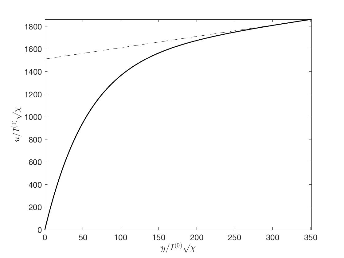
Figure 8: Velocity profile in a model steady-state shear band with $u^{\prime}_{0}=28,\>\>I^{(0)}/I_{*}=0.036,\>\>\mu_{0}=0.383,and\>\>\mu_{\infty}=0.643$.

We note that in the case of constant friction coefficient $\mu_{0}=\mu_{\infty}$ that the one-dimensional form of (11) becomes

$$2\chi u^{\prime\prime\prime\prime}-\frac{\mu_{0}p}{\surd{2}}(\mbox{sgn}(u^{\prime}))^{\prime}=0,$$ (51)

which formally involves a Dirac delta at points of transition from $u^{\prime}=0$ to $u^{\prime}\neq 0$. It is clear that the term in $\chi$ represents a singular surface traction that balances the jump in frictional stress at such points. In any case, (51) can be integrated immediately to give the odd solution in $y$ with representation appropriate to the infinite half-space $y>0$:

$$u=\left\{\begin{array}[]{ll}c_{0},\>\>\mbox{for}\>\>y>\delta,\\ p\mu_{0}y^{3}/12\surd{2}\chi+u^{\prime}_{0}y,\>\>\mbox{for}\>\>0\leq y<\delta.\end{array}\right.$$ (52)

The continuity condition $u=c_{0}$ at $y=\delta$ provides one condition on the three quantities $c_{0},\>u^{\prime}_{0}$, and $\delta$. For $u^{\prime}_{0}>0$, it follows that there is a discontinuity $p\mu_{0}\delta^{2}/4\surd{2}\chi+u^{\prime}_{0}$ in $u^{\prime}$ at $y=\delta$, leading to the Dirac delta anticipated above in (51). At any rate, upon specification of any two quantities, the solution consists of a rigid, unyielded region $y>\delta$ riding on a shear band in $0\leq y\leq\delta$. It appears that other solutions given by piecewise cubics in $y$ are possible for finite regions $0\leq y\leq L$.

Based on the preceding analysis, one can envisage solutions with any number of diffuse shear bands interspersed with more gently sheared regions, which not only reflects multiplicity of solution but is no doubt related to the mesh-size dependence in various numerical treatment of the underlying field equations (Belytschko et al., 1994).

While the above steady shear bands represents one possible solution of the steady field equations, it remains to show that they represent stable points in the space of all steady solutions.

4.1 Non-linear stability of shear bands against parallel shearing

Without attempting a full two-dimensional analysis, we consider the nonlinear stability governed by the one-dimensional form of (11) for $u(t,y)$:

$$\partial_{t}u=\partial_{y}\left[h(\partial_{y}u)-2\partial_{y}^{3}u\right],\>\>\mbox{with}\>\>h(\partial_{y}u)=\frac{1}{\surd{2}}\mu(I){\rm sgn}(\partial_{y}u),\>\>\mbox{and}\>\>I=I^{(0)}|\partial_{y}u|,$$ (53)

where $u,y$ denote the variables $\bar{u},\bar{y}$ defined in (49) and $t$ denotes the scaled time

$$\bar{t}=t/\phi I^{(0)4}\chi.$$ (54)

It is obvious that this scaling of variables restricts all parameter dependence to the function $\mu(I)$ and that the PDE (53) reduces to the rescaled ODE (45) at steady state.

To investigate the stability of the steady-state velocity $u=u_{s}(y)$, we consider the special case of an initial condition on (53) given by a perturbation of $u_{s}$. After considering several possibilities, we have settled on what appeared to be a particularly unstable perturbation represented by the sinusoidal form:

$$u(0,y)=u_{0}(y)=u_{s}(y)+A\sin k_{2}y,$$ (55)

with constant amplitude $A$ and spatial frequency $k_{2}$. We employ a standard finite-difference approximation with spatial discretization on nodal points $y_{i},\>\>i=1,\ldots,N$, with $y_{1}=0$ and with representative spacing $\Delta y_{i}$. We then employ the method of lines (MOL) (Schiesser, 2012) to solve the ODEs resulting from the discretization of (53) numerically by means of the MATLAB^®   stiff integrator ode15s.m. The details are summarized below in Appendix C, and, as pointed out there, we employ a certain number $M$ of invariant “ghost nodes” at each end of the $y$-interval at which $u(t,y_{i})=u_{s}(y_{i})$.

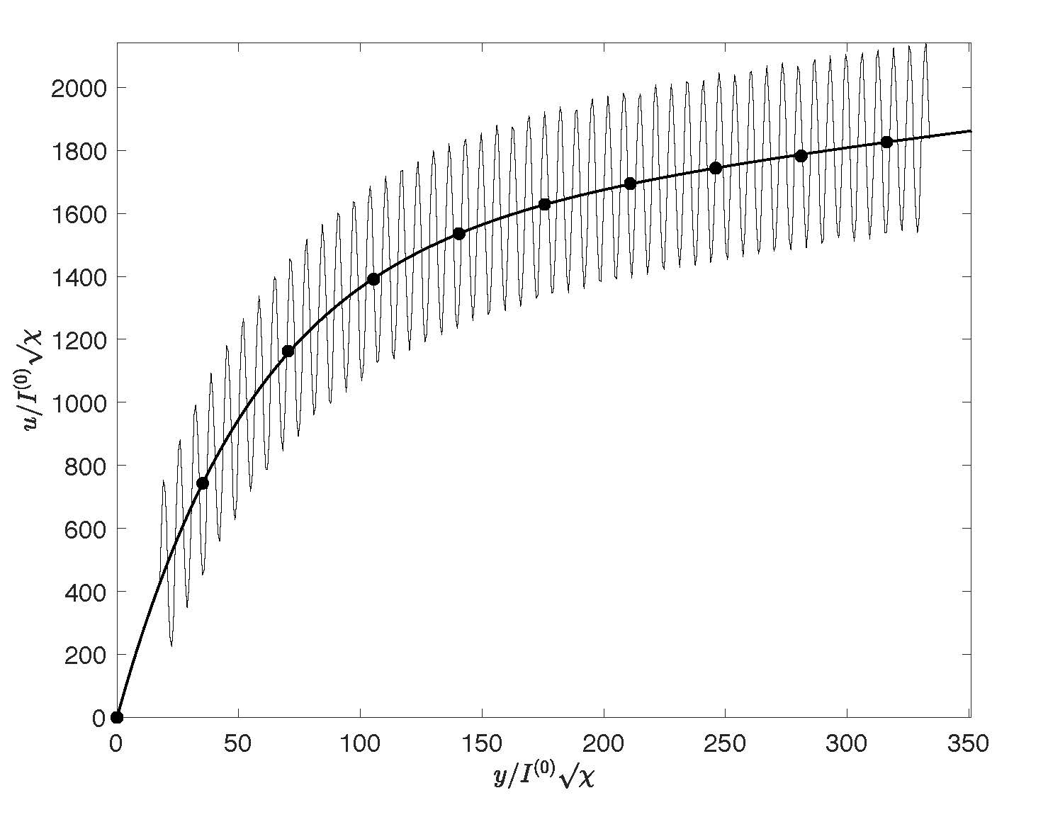
Figure 9: Stable shear band with $k_{2}=27.8$ for $u^{\prime}_{0}=28.0,\>\>I^{(0)}/I_{*}=0.036,\>\>\mu_{0}=0.3830$, and $\mu_{\infty}=0.6430$. The solid curves represent the initial steady-state and sinusoidally perturbed shear band with amplitude $A=300$, while points $\bullet$ represent the final shear band.

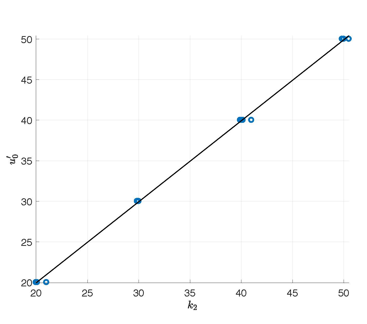
Figure 10: Maximally stable $u^{\prime}_{0}$ vs. $k_{2}$ for 72 different combinations $I^{(0)}/I*=0.1,1,10,\>\>\Delta\mu=0,0.1,0.2,0.4$, and $M=10$ ghost nodes. The number of mesh points ranged from 700 to 1000, with FDA step-size $\Delta y=0.1$, and initial guesses of the form $k_{2}=u^{\prime}_{0}=20,30,40,50$.

Stability of the initial steady state profile $u_{s}(y)$ is measured by the mean square departure $\epsilon=\sum_{i}|u(t_{\rm max},y_{i})-u_{s}(y_{i})|^{2}$ at the time $t=t_{\rm max}$ required for convergence of the unsteady solution. The most stable shear band for various values of the parameters $\mu_{0},\mu_{\infty},I^{(0)}$ can be determined by fixing one member of the pair $k_{2},u^{\prime}_{0}$, where $u^{\prime}_{0}=u^{\prime}_{s}(0)$, and minimizing $\epsilon$ with respect to the other.

However, few initial calculations revealed that $k_{2,{\rm opt}}\>\dot{=}\>u^{\prime}_{0}$, so that it is somewhat more efficient to minimize the quantity $\epsilon$ with respect to both members of the pair. This is accomplished by means of the MATLAB^®   program fminunc.m, with initial guess $k_{2}=u^{\prime}_{0}$, for various values of $u^{\prime}_{0}$. Thus, with initial guess $u^{\prime}_{0}=k_{2}=28$, one finds $u^{\prime}_{0}=28$ and $k_{2}=27.8$ as the optimal or maximally stable pair, for which the original, perturbed, and final shear bands are shown in Fig. 9. In this calculation the $y$-interval is divided into $N$ nodes, with $M<<N$ ghost nodes at each end of the interval. As indicated in Fig. 9, the sinusoidal perturbation is suppressed at the ghost nodes in order to maintain the correct boundary conditions on the unsteady solution.

Contrary to our initial hope of establishing a unique point $k_{2},u^{\prime}_{0}$, we find instead a fairly definite locus of optimal points in the $k_{2}$-$u^{\prime}_{0}$ plane with $k_{2,{\rm opt}}\dot{=}u^{\prime}_{0,{\rm opt}}$. This is summarized by the scatter plot in Fig. 10 of 72 different runs with diverse values of the various parameters. The least-squares straight line shown there is given by $u^{\prime}_{0}=0.998k_{2}$ whose rms fractional error is approximately 1%. Remarkably the results appear to be almost independent of the sinusoidal-perturbation amplitude $A$, although $A$ does have some influence on the convergence of the unsteady solution.

For completeness, we have also investigated the stability of the homogenous shear field with above sinusoidal perturbation, i.e. the stability of the state with $u_{s}=y$ in (55). With $u=0$ imposed at $y=0$ as the only constraint, we find unbounded growth near $y=0$ without achieving a profile that resembles our steady shear band. Although one might conclude that our steady shear band does not represent a general point of attraction in the space of steady-state solutions, and is perhaps attainable only through 2D effects, we are inclined to attribute the form of the instability to our finite-difference implementation of the method of lines. While it would be interesting to employ more robust spectral methods, this would take us well beyond the scope of the present paper.

5 Pure Shear

To illustrate the effects of base-state shearing, we consider a base state defined by $\mathbf{v}^{(0)}=(x_{1},-x_{2})/2$, with

$$\mathbf{D}^{(0)}\equiv\mathbf{L}^{(0)}=\frac{1}{\surd{2}}{\bf E^{(0)}}=\frac{1}{2}\left[\begin{array}[]{cc}1&0\\ 0&-1\end{array}\right],$$ (56)

Hence, for planar disturbances the relation for $\mathbf{k}(t,\boldsymbol{\kappa})$ in (23) becomes

$$\mathbf{k}=\exp(-t\mathbf{L}^{(0)T})\boldsymbol{\kappa},\>\>\mbox{with}\>\>k_{1}=\kappa_{1}\kappa_{2}/k_{2},\mbox{and}\>\>\>k_{2}=\kappa_{2}\exp(t/2)$$ (57)

Then, by the methods employed above, we find the eigenvalue $\lambda$ of $\mathbf{A}$ with largest real part to be

$$\begin{split}&\lambda=\frac{1}{2\phi\Phi_{1}}\left[4\beta\gamma k_{1}^{2}k_{2}^{2}-2\Phi_{1}\Phi_{2}+\phi(k_{1}^{2}-k_{2}^{2}-\frac{\alpha}{\surd{2}}k^{2})+\Phi_{3}^{1/2}\right],\\ &\mbox{where}\>\>\Phi_{1}=(1-\frac{\alpha}{\surd 2})k_{1}^{2}+(1+\frac{\alpha}{\surd 2})k_{2}^{2},\\ &\mbox{and}\>\>\Phi_{3}=2k_{1}^{2}k_{2}^{2}\>[8\beta^{2}\gamma^{2}k_{1}^{2}k_{2}^{2}+4\beta\gamma\phi(k_{1}^{2}-k_{2}^{2}-\alpha k^{2}/\surd{2})+\phi^{2}(\alpha^{2}-2)].\end{split}$$ (58)

When convection is neglected, we find that

$$\Phi_{3}=16\beta^{2}\gamma^{2}k_{1}^{4}k_{2}^{4},\>\>\mbox{and}\>\>\lambda=\frac{4\beta\gamma k_{1}^{2}k_{2}^{2}-\Phi_{1}\Phi_{2}}{\phi\Phi_{1}}.$$ (59)

Fig.​ 11 shows the effects of $\chi$ and convection on stability, and Fig.​ 12 illustrates oscillatory behavior. Note that the unstable regions in both figures are rotated at approximately $45^{\circ}$ relative to the corresponding regions for simple shear, which is relevant to the associated shear-band models.

Oscillatory behavior occurs when $\Phi_{3}<0$ in (58), or in the region

$$8\beta^{2}\gamma^{2}k_{1}^{2}k_{2}^{2}+4\beta\gamma\phi(k_{1}^{2}-k_{2}^{2}-\alpha k^{2}/\surd{2})+\phi^{2}(\alpha^{2}-2)<0,$$ (60)

whose boundaries are readily found to be

$$k_{1}=\pm\left[\frac{\phi}{2\beta\gamma}\left(1+\frac{\alpha}{\surd{2}}\right)\right]^{1/2},$$ (61)

upon solving for $k_{2}^{2}$ in terms of $k_{1}^{2}$. These are shown in the stability diagram of Fig.​ 12, where, in contrast to simple shear, there now exist both stable and unstable oscillations.

Since $k_{1}k_{2}=\kappa_{1}\kappa_{2}$, a constant, from (57), the asymptotic behavior with or without convection is stable,

$$\lambda\sim-\frac{1}{\phi}\Phi_{2}\sim-\frac{1}{\phi}(\gamma k_{2}^{2}+2\chi k_{2}^{4}),\>\>\mbox{for}\>\>t\rightarrow\infty,$$ (62)

with relative error $O(k_{2}^{-2})=O(e^{t})$. Clearly, we have stability even for $\chi=0$.

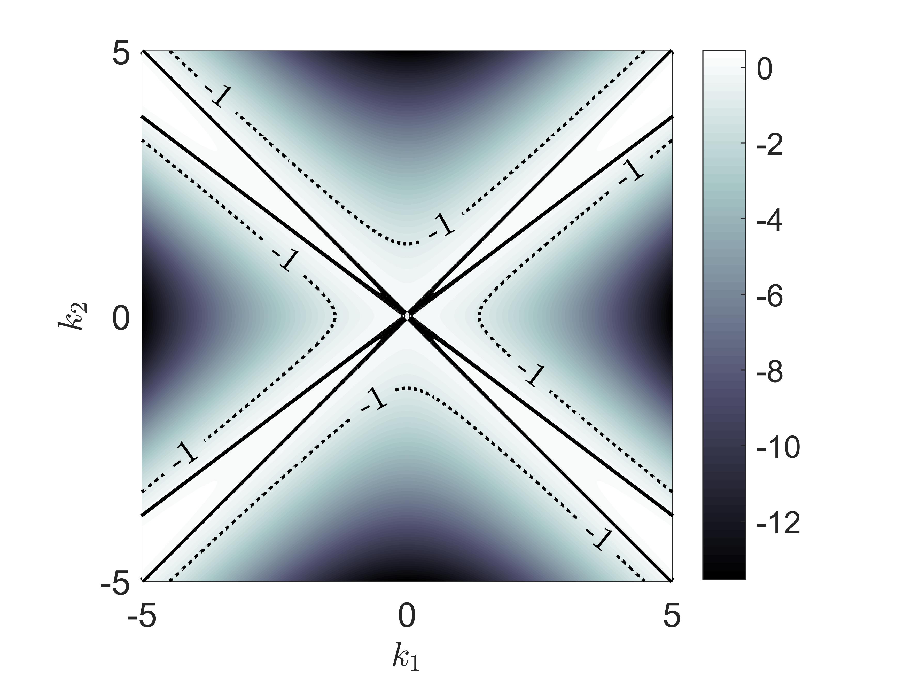
(a)

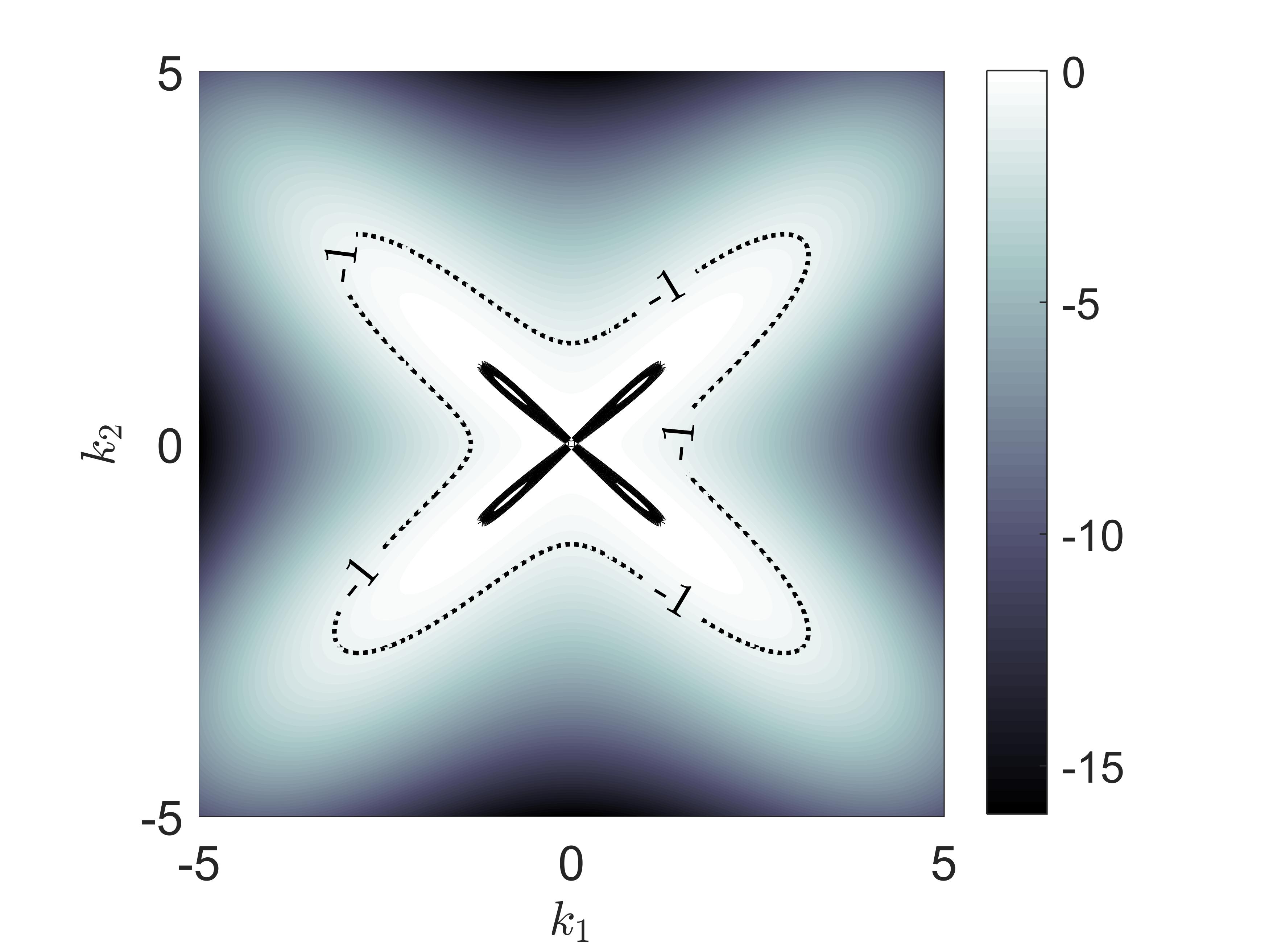
(b)

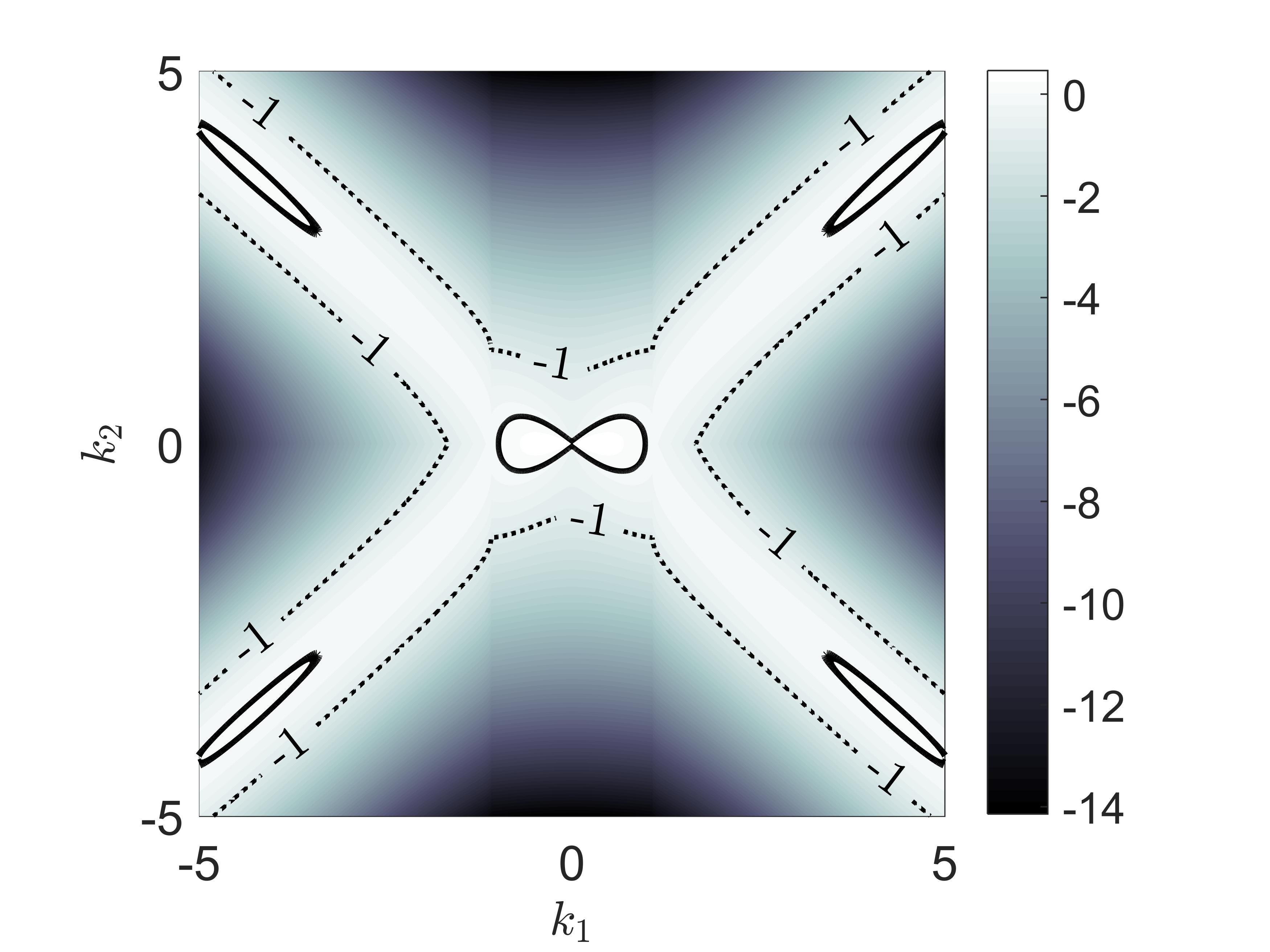
(c)

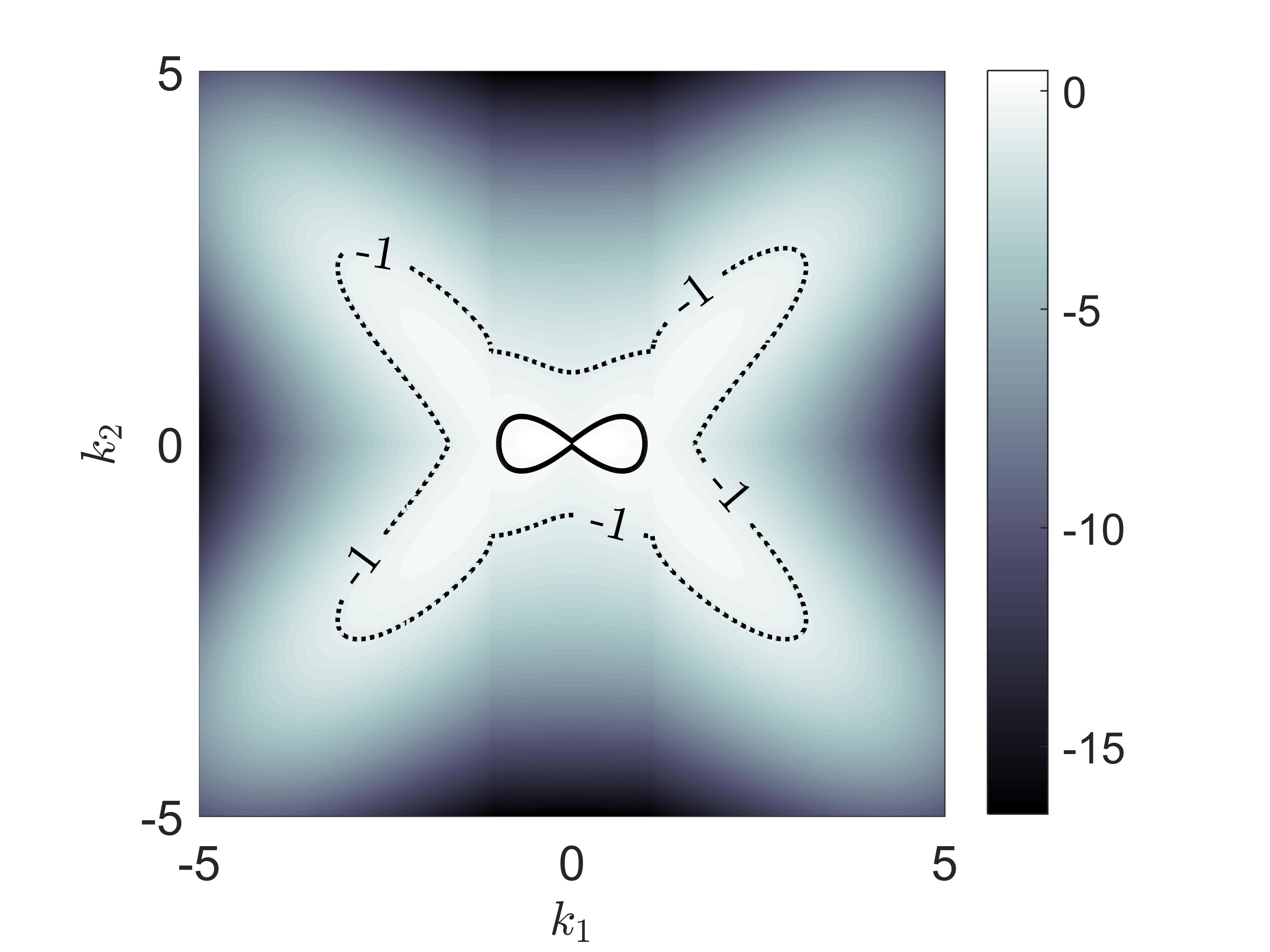
(d)

Figure 11: Stability for pure shear without convection, for $\chi$ values (a) $0$ (b) $0.001$, and with convection, for $\chi$ values (c) $4\times 10^{-5}$ and (d) $0.001$, for $I=0.0001$, $\phi=0.5$, and $p^{(0)}=1$.

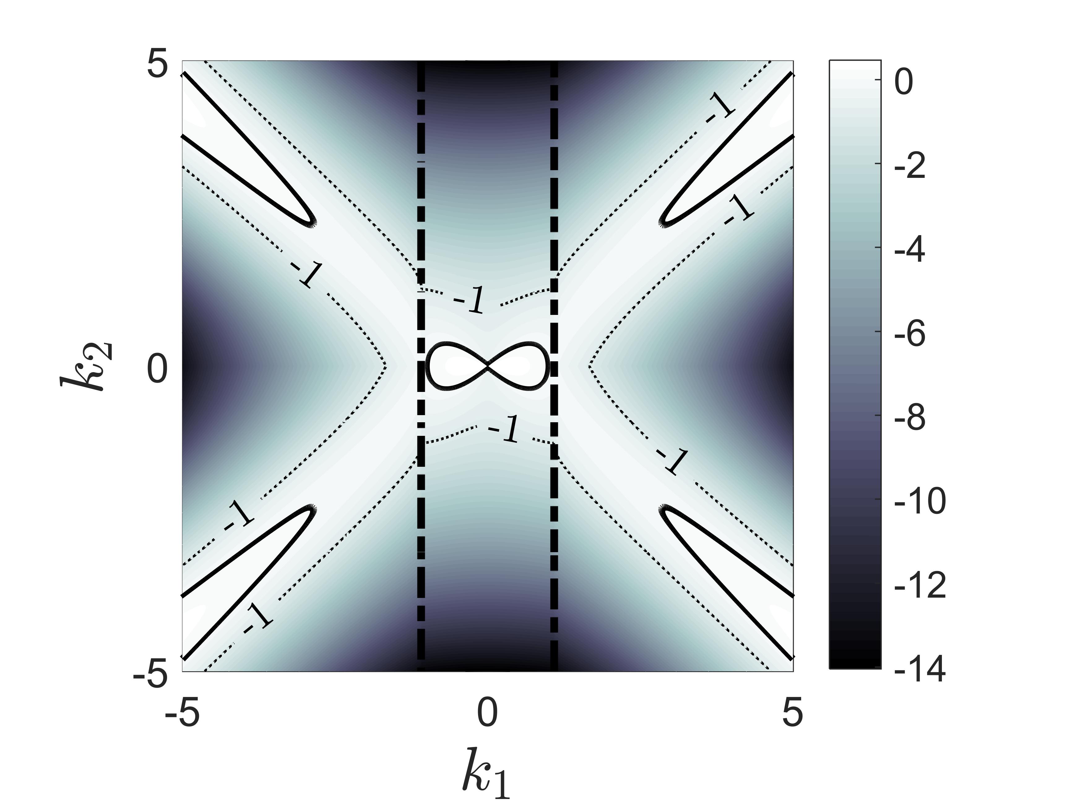
Figure 12: Oscillatory behavior for pure shear resulting from convection, for $\chi=0$, $\textit{I}=0.0001$, $p^{(0)}=1$, and $\phi=0.5$. The oscillation frequency is non-zero within the central regions bounded by dash-dotted vertical lines. Solid and dotted curves are contours of the real part of $\lambda$, with the former representing neutral stability.

Once again, one may derive a model for the shear band resulting from material instability. Thus, making use once more of the of the MATLAB^® program “fminunc” to determine numerically the unconstrained minimum in $-\lambda(\mathbf{k})$, for parameter values $\mu_{0}=0.383,\mu_{\infty}=0.643,I_{*}=0.279,I^{(0)}=0.001,\chi=10^{-6}$ we find $\mathbf{k}_{\rm max}\approx\pm(26.0,22.5)$. This corresponds roughly to the classical $\approx 45^{\circ}$ shear-band orientation found in previous experiments and numerical simulations. Figure 13 shows the growth of the Fourier mode, and it is seen from panel (b) that the transient growth can become quite large before being quenched by a combination of wavevector stretching and damping by higher gradients.

The above result leads us to express (11), with ${\bf g}=0$ and $\nabla p$, on a coordinate system oriented at $45^{\circ}$ to that involved in (56), reducing it to the form (45) and (56) to the form (25). Therefore, the analysis of the shear band reduces essentially to that of Section 4, with appropriate modification of the boundary condition on $u^{\prime}(0)$. On this new coordinate system, the above value of $\mathbf{k}_{\rm max}$ becomes $\approx\pm(2,34)$ as opposed to the value $\pm(2,28)$ found in Section 4 for simple shear. Given the rough agreement of these values and in light of the non-unique solution to our shear-band model, it hardly seems worthwhile to repeat the calculation leading to Fig. 8 with an only slightly modified boundary condition on $u^{\prime}(0)$.

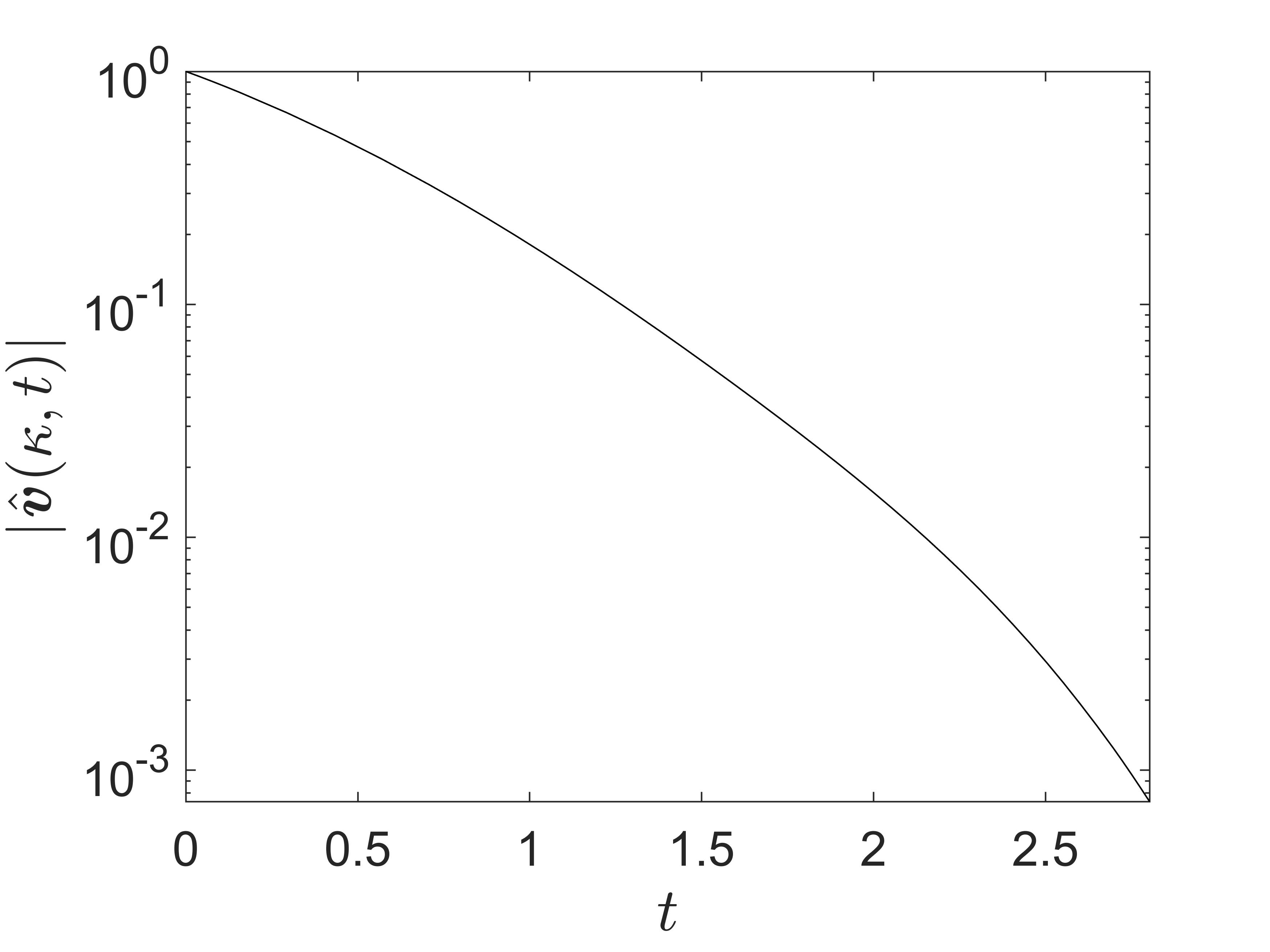
(a)

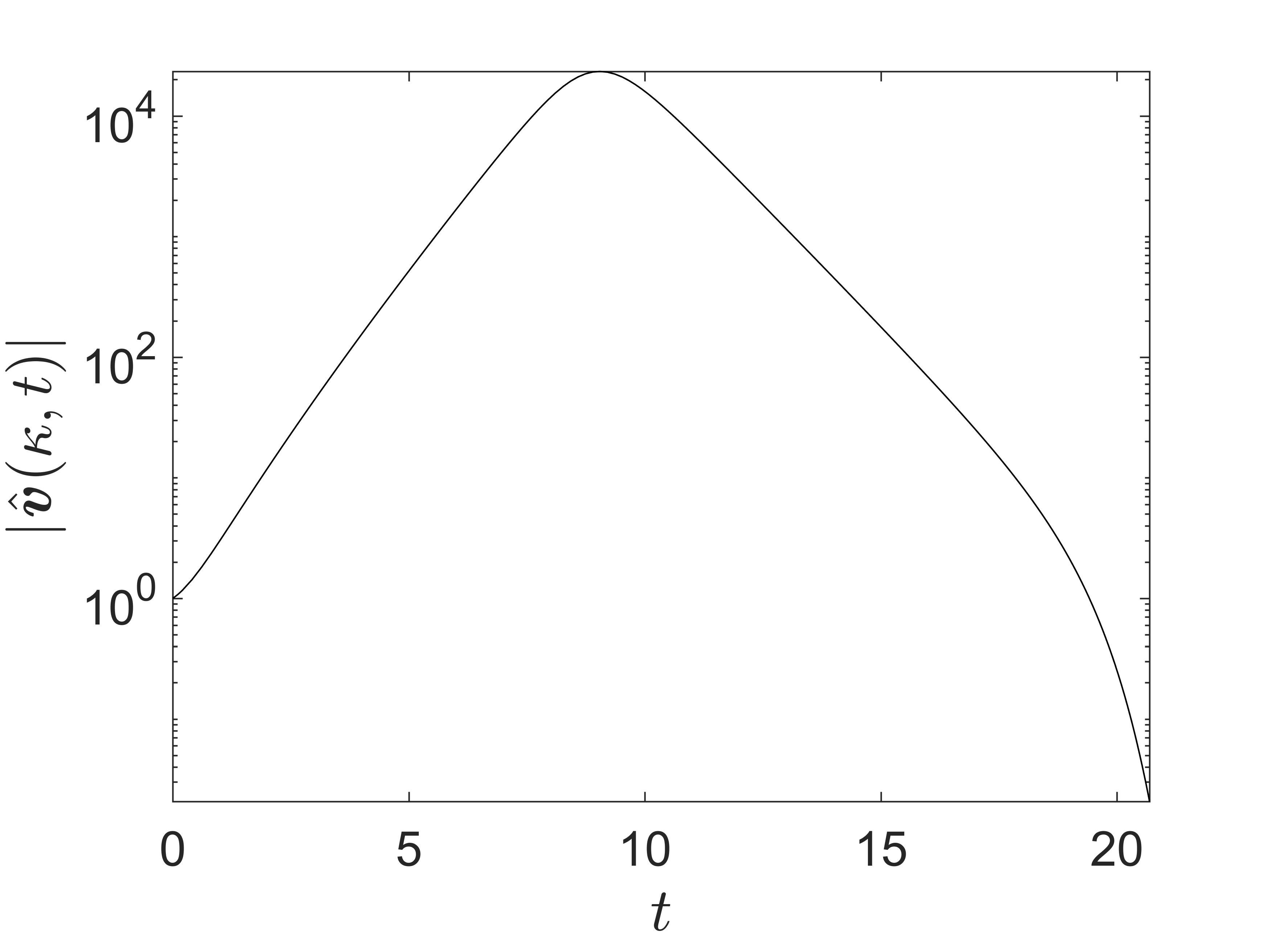
(b)

Figure 13: Magnitude $|\hat{\boldsymbol{\upsilon}}(\boldsymbol{\kappa},t)|$ of initially stable and unstable Fourier modes vs. $t$ for planar pure shear for $\chi=10^{-6}$ and initial conditions (a) $\boldsymbol{\kappa}=(-0.5,-0.866)$,; (b) $\boldsymbol{\kappa}=(1,0.0001)$.

6 Concluding Remarks

Our major findings are adequately summarized in the Abstract and Introduction. To briefly recapitulate the most important of these, we find for both planar simple shear and pure shear that the linear instability of the $\mu(I)$ model identified by Barker et al. (2015) is modified through convection by the base flow, giving way to long-time stability induced by Kelvin wave-vector stretching. The addition of gradient effects via the vdW-CH model provides a wave-number cut-off that serves to stabilize the dynamical equations over the entire time domain, to regularize the quasi-static field equations, and to assign a diffuse length scale to eventual shear bands.

We find that steady shear bands are stable against steady parallel sinusoidal shear fields, provided the normal velocity gradient of the shear band is very nearly equal to the wave number of the sinusoidal perturbation. To obtain a unique shear band, it is necessary to assume some preferred wave number, e.g. the most unstable one according to linear theory. A challenge for future work is to elucidate shear band formation in the presence of more complex spatial perturbations to homogenous shearing.

In summary, we conclude that the (Hadamard) short wave length instability found by Barker et al. (2015) is connected to the loss of ellipticity in the quasi-static field equations. Although transient and eventually quenched by wave vector stretching according to linear theory, the instability is doubtless problematical for numerical simulation and it may also trigger non-linear instabilities. Addition of higher-gradient effects like those considered in the present work should go a long way towards alleviating such problems.

As a practical matter, the present work may suggest a stratagem for numerical simulation of materially unstable visco-plasticity, in which a transient form of the vdW-CH or similar regularization is invoked to minimize transient instabilities, with the possibility of describing the structure of shear bands on longer time scales if so desired. Our simple model of a shear band based on the vdW-CH model suggests that spatial boundary conditions, required in principle by any higher-gradient model, can be chosen somewhat arbitrarily, as the higher gradients tend to have a spatially localized domain of influence.

As additional future work, it would be worthwhile to apply the current theory to other homogeneous shear flows, such as axisymmetric straining of the kind that arises in the standard quasi-static tests of soil mechanics or in more rapid converging-hopper flows. While somewhat distinct from the issue of material instability, an investigation should be carried out of the coupling of pressure gradients in the base flow to the perturbed momentum balance, an effect neglected in Ref.​ 1 and the present study.

As a deeper theoretical issue, it would be interesting to investigate the possible relation between the weakly non-local model of the present study and the fully non-local variants of the $\mu(I)$ model proposed by Pouliquen & Forterre (2009) and more recently by Kamrin and co-workers (See e.g. Henann & Kamrin, 2014). We recall that the latter model can be tied to a Ginzburg-Landau formalism, which shares a certain kinship to the vdW-Cahn-Hilliard model of the present study (Gurtin, 1996).

Appendix A Derivation of the perturbed equations (17)

Substituting (15) and (16) into (13), the perturbed equations of motion become

$$\begin{split}&\rho_{s}\phi\left(\partial_{t}\mathbf{v}^{(1)}+\mathbf{v}^{(0)}\!\cdot\!\nabla\mathbf{v}^{(1)}+\mathbf{v}^{(1)}\!\cdot\!\nabla\mathbf{v}^{(0)}\right)=-\nabla p^{(1)}\\ &+\frac{(2-\stackrel{{\scriptstyle\>\prime}}{{\mu}}^{(0)})\mu^{(0)}}{2}\mathbf{E}^{(0)}\nabla p^{(1)}+\left[\left(\frac{\partial\mu}{\partial p}\right)^{(0)}p^{(1)}+\left(\frac{\partial\mu}{\partial\mathbf{D}}\right)^{(0)}\!\cdot\!\nabla\mathbf{v}^{(1)}\right]\mathbf{E}^{(0)}\nabla p^{(0)}\\ &-\frac{1}{2}\left\{\mu^{(0)}\left[{\left(\frac{\partial\stackrel{{\scriptstyle\>\prime}}{{\mu}}}{\partial p}\right)}^{(0)}p^{(1)}+{\left(\frac{\partial\stackrel{{\scriptstyle\>\prime}}{{\mu}}}{\partial\mathbf{D}}\right)}^{(0)}\!\cdot\!\nabla\mathbf{v}^{(1)}\right]\right.\\ &\left.+\stackrel{{\scriptstyle\>\prime}}{{\mu}}^{(0)}\left[\left(\frac{\partial\mu}{\partial p}\right)^{(0)}p^{(1)}+\left(\frac{\partial\mu}{\partial\mathbf{D}}\right)^{(0)}\!\cdot\!\nabla\mathbf{v}^{(1)}\right]\right\}\mathbf{E}^{(0)}\nabla p^{(0)}\\ &+\frac{(\stackrel{{\scriptstyle\>\prime}}{{\mu}}^{(0)}-1)\mu^{(0)}p^{(0)}}{|\mathbf{D}^{(0)}|}(\mathbf{E}^{(0)}\nabla)(\mathbf{E}^{(0)}\!\cdot\!\nabla\mathbf{v}^{(1)})+\frac{\mu^{(0)}p^{(0)}}{2|\mathbf{D}^{(0)}|}\nabla^{2}\mathbf{v}^{(1)}-2\chi\nabla^{4}\mathbf{v}^{(1)},\end{split}$$ (63)

where

$$\begin{split}\left(\frac{\partial\mu}{\partial p}\right)^{(0)}&=\left(\frac{\mathop{}\mathrm{d}\mu}{\mathop{}\mathrm{d}I}\frac{\partial I}{\partial p}\right)^{(0)}=\left(-\frac{I}{2p}\frac{\mathop{}\mathrm{d}\mu}{\mathop{}\mathrm{d}I}\right)^{(0)}=-\frac{\mu^{(0)}\stackrel{{\scriptstyle\>\prime}}{{\mu}}^{(0)}}{2p^{(0)}},\>\>\\ \left(\frac{\partial\stackrel{{\scriptstyle\>\prime}}{{\mu}}}{\partial p}\right)^{(0)}&=\left[\frac{\partial I}{\partial p}\left(\frac{1}{\mu}\frac{\mathop{}\mathrm{d}\mu}{\mathop{}\mathrm{d}I}-\frac{I}{\mu^{2}}\left(\frac{\mathop{}\mathrm{d}\mu}{\mathop{}\mathrm{d}I}\right)^{2}+\frac{I}{\mu}\frac{\mathop{}\mathrm{d}^{2}\mu}{\mathop{}\mathrm{d}I^{2}}\right)\right]^{(0)}\\ &=-\frac{1}{2p^{(0)}}\left[\stackrel{{\scriptstyle\>\prime}}{{\mu}}^{(0)}-(\stackrel{{\scriptstyle\>\prime}}{{\mu}}^{(0)})^{2}+\stackrel{{\scriptstyle\>\prime\prime}}{{\mu}}^{(0)}\right],\\ \left(\frac{\partial\mu}{\partial\mathbf{D}}\right)^{(0)}&=\left(\frac{\mathop{}\mathrm{d}\mu}{\mathop{}\mathrm{d}I}\frac{\partial I}{\partial\mathbf{D}}\right)^{(0)}=\left(I\frac{\mathop{}\mathrm{d}\mu}{\mathop{}\mathrm{d}I}\frac{\mathbf{E}}{|\mathbf{D}|}\right)^{(0)}=\mu^{(0)}\stackrel{{\scriptstyle\>\prime}}{{\mu}}^{(0)}\frac{\mathbf{E}^{(0)}}{|\mathbf{D}^{(0)}|},\\ \left(\frac{\partial\stackrel{{\scriptstyle\>\prime}}{{\mu}}}{\partial\mathbf{D}}\right)^{(0)}&=\left[\frac{\partial I}{\partial\mathbf{D}}\left(\frac{1}{\mu}\frac{\mathop{}\mathrm{d}\mu}{\mathop{}\mathrm{d}I}-\frac{I}{\mu^{2}}\left(\frac{\mathop{}\mathrm{d}\mu}{\mathop{}\mathrm{d}I}\right)^{2}+\frac{I}{\mu}\frac{\mathop{}\mathrm{d}^{2}\mu}{\mathop{}\mathrm{d}I^{2}}\right)\right]^{(0)}\\ &=\left[\stackrel{{\scriptstyle\>\prime}}{{\mu}}^{(0)}-(\stackrel{{\scriptstyle\>\prime}}{{\mu}}^{(0)})^{2}+\stackrel{{\scriptstyle\>\prime\prime}}{{\mu}}^{(0)}\right]\frac{\mathbf{E}^{(0)}}{|\mathbf{D}^{(0)}|}.\end{split}$$ (64)

Rearranging (63) and making use of (64) gives

$$\begin{split}&\rho_{s}\phi\left(\partial_{t}\mathbf{v}^{(1)}+\mathbf{v}^{(0)}\!\cdot\!\nabla\mathbf{v}^{(1)}+\mathbf{v}^{(1)}\!\cdot\!\nabla\mathbf{v}^{(0)}\right)=-\nabla p^{(1)}+\frac{(2-\stackrel{{\scriptstyle\>\prime}}{{\mu}}^{(0)})\mu^{(0)}}{2}\mathbf{E}^{(0)}\nabla p^{(1)}\\ &+\frac{(\stackrel{{\scriptstyle\>\prime}}{{\mu}}^{(0)}-1)\mu^{(0)}p^{(0)}}{|\mathbf{D}^{(0)}|}(\mathbf{E}^{(0)}\nabla)(\mathbf{E}^{(0)}\!\cdot\!\nabla\mathbf{v}^{(1)})+\frac{\mu^{(0)}p^{(0)}}{2|\mathbf{D}^{(0)}|}\nabla^{2}\mathbf{v}^{(1)}-2\chi\nabla^{4}\mathbf{v}^{(1)}\\ &+\left[\frac{\mu^{(0)}(\stackrel{{\scriptstyle\>\prime\prime}}{{\mu}}^{(0)}-\stackrel{{\scriptstyle\>\prime}}{{\mu}}^{(0)})}{4p^{(0)}}p^{(1)}+\frac{\mu^{(0)}}{2|\mathbf{D}^{(0)}|}(\stackrel{{\scriptstyle\>\prime}}{{\mu}}^{(0)}-\stackrel{{\scriptstyle\>\prime\prime}}{{\mu}}^{(0)})\mathbf{E}^{(0)}\!\cdot\!\nabla\mathbf{v}^{(1)}\right]\mathbf{E}^{(0)}\nabla p^{(0)}.\end{split}$$ (65)

Appendix B A Squire’s-type theorem for $\mu(I)$-rheology

Allowing for out-of-plane perturbations, the components of the tensors in (27) are given by

$$\begin{split}\mathbf{I}\!-\!\frac{\mathbf{N}^{(0)}\mathbf{k}\otimes\mathbf{k}}{\mathbf{k}\!\cdot\!{\bf N}^{(0)}\mathbf{k}}&\!=\!\frac{1}{\Phi_{1}}\!\begin{bmatrix}\Phi_{1}\!+\!k_{1}\!\left(\!\frac{\alpha}{\sqrt{2}}k_{2}\!-\!k_{1}\!\right)&&\!\!\!\!\!\!k_{2}\left(\frac{\alpha}{\sqrt{2}}k_{2}\!-\!k_{1}\!\right)&&\!\!\!\!\!\!k_{3}\left(\frac{\alpha}{\sqrt{2}}k_{2}\!-\!k_{1}\!\right)\\ k_{1}\left(\!\frac{\alpha}{\sqrt{2}}k_{1}\!-\!k_{2}\!\right)&&\!\!\!\!\!\!\Phi_{1}\!+\!k_{2}\left(\!\frac{\alpha}{\sqrt{2}}k_{1}\!-\!k_{2}\!\right)&&\!\!\!\!\!\!k_{3}\left(\!\frac{\alpha}{\sqrt{2}}k_{1}\!-\!k_{2}\!\right)\\ -k_{1}k_{3}&&-k_{2}k_{3}&&\Phi_{1}-k_{3}^{2}\end{bmatrix},\\ {\bf M}\!-\!{\bf L}^{(0)}\!&=\!\frac{1}{\phi}\begin{bmatrix}\beta\gamma k_{2}^{2}&\beta\gamma k_{1}k_{2}\!-\!2\phi&0\\ \beta\gamma k_{1}k_{2}&\beta\gamma k_{1}^{2}&0\\ 0&0&0\end{bmatrix}\end{split}$$ (66)

where $\Phi_{1}=\mathbf{k}\!\cdot\!{\bf N}^{(0)}\mathbf{k}$, and $k^{2}=k_{2D}^{2}+k_{3}^{2}$, $k_{2D}^{2}=k_{1}^{2}+k_{2}^{2}$, and $\Phi_{2}=\gamma k^{2}+2\chi k^{4}$.

Making use of the relation $\det(\mathbf{A}-\lambda\mathbf{I})=0$, the eigenvalues $\lambda$ of $\mathbf{A}$ are found to be

$$\begin{split}&\lambda_{{\textrm{\scriptsize 1}}\atop{\textrm{\scriptsize 2}}}=\frac{\beta\gamma[(k_{1}^{2}-k_{2}^{2})^{2}+k_{3}^{2}k_{2D}^{2}]-2\Phi_{1}\Phi_{2}\pm{\Phi_{4}}^{1/2}}{2\phi\Phi_{1}},\\ &\lambda_{3}=-\frac{\Phi_{2}}{\phi}=-\frac{1}{\phi}\left(\gamma k^{2}+2\chi k^{4}\right),\end{split}$$ (67)

where

$$\begin{split}\Phi_{4}=&\beta^{2}\gamma^{2}(k_{1}^{2}\!-\!k_{2}^{2})^{4}\!+\!2\phi^{2}k_{1}^{2}(\!\alpha k_{1}\!-\!\sqrt{2}k_{2}\!)^{2}\!-\!2\beta\gamma\phi k_{1}^{2}(k_{1}^{2}\!-\!k_{2}^{2})(\!\sqrt{2}\alpha k_{1}^{2}\!-\!4k_{1}k_{2}\!+\!\sqrt{2}\alpha k_{2}^{2})\\ &+k_{3}^{2}\left[\beta^{2}\gamma^{2}k_{2D}^{2}(k_{3}^{2}k_{2D}^{2}\!+\!2(k_{1}^{2}-k_{2}^{2})^{2})\!+\!2\beta\gamma\phi k_{1}[(k_{1}^{2}-k_{2}^{2})(2k_{2}\!-\!\sqrt{2}\alpha k_{1})\!-\!2k_{2}k_{3}^{2}]\right].\end{split}$$

Comparison of the three eigenvalues indicates that the in-plane eigenvalue $\lambda_{1}$ has largest real part, so that planar disturbances are the least stable,Q.E.D..

Appendix C Numerical solution of (53)

To solve (53) numerically we employ the well-known method of lines (MOL) (Schiesser, 2012), with spatial discretization at $N$ nodal points in $y$, converting (53) to a set of ODEs that can be solved by standard solvers. Specifically, we choose a standard finite-difference approximation with

$$\begin{split}&y\rightarrow[y_{i}],\>u(t,y)\rightarrow\underline{u}(t)\!=\![u_{i}(t)],\>\partial^{m}_{y}u\rightarrow\underline{D}^{(m)}\underline{u}\!=\![D^{(m)}_{ij}u_{j}],\>\mbox{with}\>u_{i}(t)\!=\!u(t,y_{i}),\\ &\mbox{for}\>i,j\!=\!1,\ldots,N,\>\mbox{and}\>\frac{\mathop{}\mathrm{d}\underline{u}}{\mathop{}\mathrm{d}t}\!=\!\underline{D}^{(1)}\left(\underline{h}-2\underline{D}^{(3)}\underline{u}\right),\>\mbox{with}\>\>h_{i}\!=\!h(D^{(1)}_{ij}u_{j}),\end{split}$$ (68)

where the rows of the matrices $\underline{D}^{(m)}$ are given by the classic interpolation coefficients of Fornberg (1988), generalized to an arbitrary number of interpolation points $P>m$. To generate these coefficients for $m=1,3$ we have made use of the third-party MATLAB^®   program “fdcoeffF.m”.

We employ the MATLAB^®   stiff integrator “ode15s.m” to integrate the N-dimensional ODE in subject to the initial condition $\underline{u}(0)=\underline{u}_{0}=[u_{0}(y_{i})]$ given by (55). We note that for the above ODE, it is rather easy to derive the analytical Jacobian, which is essentially the same as the matrix defining linear stability.

To satisfy the spatial boundary at the ends of the interval $(y_{1},y_{N})$ we employ $M$ “ghost nodes” $y_{1},\ldots,y_{M}$ and $y_{N-M+1},\ldots,y_{N}$ at either end, where $u_{i}(t)=u_{s}(y_{i})$ for all $t>0$. To enforce this condition on the ODE solver, we we set the top and bottom $M$ rows of $\underline{D}^{(1)}$ equal to zero, i.e. $D^{(1)}_{i,j}=0$, for $\>\>i=1,\ldots,M$ and $i=N-M+1,\ldots,N$, and we adopt the modified initial condition

$$u_{0}(y_{i})=u_{s}(y_{i})+R(y_{M+1},y_{N-M})A\sin k_{2}y_{i},$$ (69)

where $R$ denotes the rectangular pulse vanishing on the ghost nodes and otherwise equal to unity. This leaves $N-2M$ “active” nodes, and we choose $P=2M$ as the number of Fornberg interpolation points, so that interpolation on the $N-P$ active nodes in the center of the interval (0,1) may include up to $M$ ghost node at either end.

The ODE solver is run for a preset time $t=t_{\rm max}$, long enough to ensure convergence of $\underline{u}(t)$. As indicated above in Subsection 4.1, we employ as measure of stability of $\underline{u}_{s}$ the mean of $\epsilon=|\underline{u}(t_{\rm max})-\underline{u}_{s}|^{2}$, as given by the MATLAB^®   function “std.m”. For total number of nodes $\approx 1000$ on the $y$-interval (0, 1) we find a nearly neglible effect of the number $M$ of ghost nodes, with $M$ ranging from $10$ to $50$.

References

- Alam & Nott (1997) Alam, M & Nott, P 1997 The influence of friction on the stability of unbounded granular shear flow. J. Fluid Mech. 343, 267–301.
- Anderson et al. (1998) Anderson, D. M., McFadden, G. B. & Wheeler, A. A. 1998 Diffuse-interface methods in fluid mechanics. Ann. Rev. Fluid Mech. 30 (1), 139–165.
- Barker & Gray (2017) Barker, T & Gray, N 2017 Partial regularisation of the incompressible -rheology for granular flow. J. Fluid Mech. 828, 5–32.
- Barker et al. (2015) Barker, T, Schaeffer, DG, Bohorquez, P & Gray, JMNT 2015 Well-posed and ill-posed behaviour of the-rheology for granular flow. J. Fluid Mech. 779, 794–818.
- Barker et al. (2017) Barker, T., Schaeffer, D., Shearer, M. & Gray, N. 2017 Well-posed continuum equations for granular flow with compressibility and (i)-rheology. Proc. R. Soc. A 473 (2201), 20160846.
- Belytschko et al. (1994) Belytschko, T, Chiang, H-Y & Plaskacz, E 1994 High resolution two-dimensional shear band computations: imperfections and mesh dependence. Comp. Meth. Appl. Mech. Eng. 119 (1-2), 1–15.
- Bigoni (1995) Bigoni, D 1995 On flutter instability in elastoplastic constitutive models. Int. J. Solids Structs. 32 (21), 3167–3189.
- Brezis & Browder (1998) Brezis, H & Browder, F 1998 Partial differential equations in the 20th century. Adv. Math. 135 (1), 76–144.
- Browder (1961) Browder, F 1961 On the spectral theory of elliptic differential operators. I. Math. Ann. 142 (1), 22–130.
- Cahn & Hilliard (1958) Cahn, J W & Hilliard, J E 1958 Free energy of a nonuniform system. I. interfacial free energy. J. Chem. Phys. 28 (2), 258–267.
- Didwania & Goddard (1993) Didwania, A K & Goddard, J D 1993 A note on the generalized Rayleigh quotient for non-self-adjoint linear stability operators. Phys. Fluids A 5 (5), 1269–1271.
- Edelen (1972) Edelen, D. G. B. 1972 A nonlinear Onsager theory of irreversibility. Int. J. Eng. Sci. 10 (6), 481–90.
- Edelen (2005) Edelen, D G B 2005 Applied exterior calculus. Mineola, NY: Dover Publications Inc.
- Forest & Aifantis (2010) Forest, S & Aifantis, E 2010 Some links between recent gradient thermo-elasto-plasticity theories and the thermomechanics of generalized continua. Int. J. Solids Structs. 47 (25), 3367–3376.
- Fornberg (1988) Fornberg, B. 1988 Generation of finite difference formulas on arbitrarily spaced grids. Mathematics of computation 51 (184), 699–706.
- Goddard (2003) Goddard, J D 2003 Material instability in complex fluids. Ann. Rev. Fluid Mech. 35 (1), 113–133.
- Goddard (2014) Goddard, J D 2014 Edelen’s dissipation potentials and the visco-plasticity of particulate media. Acta Mech. 225 (8), 2239–2259.
- Gurtin (1996) Gurtin, M E 1996 Generalized Ginzburg-Landau and Cahn-Hilliard equations based on a microforce balance. Physica D 92 (3), 178–192.
- Henann & Kamrin (2014) Henann, D L & Kamrin, K 2014 Continuum thermomechanics of the nonlocal granular rheology. Int. J. Plasticity 60, 145–162.
- Heyman et al. (2017) Heyman, J, Delannay, R, Tabuteau, H & Valance, A 2017 Compressibility regularizes the (i)-rheology for dense granular flows. J. Fluid Mech. 830, 553–568.
- Hill (1956) Hill, R. 1956 New horizons in the mechanics of solids. J. Mech. Phys. Solids 5 (1), 66–74.
- Jop et al. (2005) Jop, P, Forterre, Y & Pouliquen, O 2005 Crucial role of sidewalls in granular surface flows: consequences for the rheology. J. Fluid Mech. 541, 167–192.
- Jop et al. (2006) Jop, P, Forterre, Y & Pouliquen, O 2006 A constitutive law for dense granular flows. Nature 441 (7094), 727–730.
- Leonov (1988) Leonov, A. I. 1988 Extremum principles and exact two-side bounds of potential: Functional and dissipation for slow motions of nonlinear viscoplastic media. J. Non-Newton. Fluid Mech. 28 (1), 1–28.
- MiDi (2004) MiDi, GDR 2004 On dense granular flows. Europ. Phys. J. E 14 (4), 341–365.
- Mindlin (1964) Mindlin, R D 1964 Micro-structure in linear elasticity. Arch. Ration. Mech. Anal. 16 (1), 51–78.
- Pouliquen & Forterre (2009) Pouliquen, O & Forterre, Y 2009 A non-local rheology for dense granular flows. Phil. Trans. Roy. Soc. Lond. A 367 (1909), 5091–5107.
- Renardy & Rogers (2006) Renardy, M & Rogers, R 2006 An introduction to partial differential equations. Springer Science.
- Rowlinson (1979) Rowlinson, J S 1979 Translation of J D van der Waals’ “The thermodynamik theory of capillarity under the hypothesis of a continuous variation of density”. J. Stat. Phys. 20 (2), 197–200.
- Saramito (2016) Saramito, P. 2016 Complex Fluids - Modeling and Algorithms. SMAI/Springer Int. Publishing.
- Schiesser (2012) Schiesser, W. E. 2012 The numerical method of lines: integration of partial differential equations. Elsevier.
- Thomson (1887) Thomson, W 1887 XXI. Stability of fluid motions (continued from the May and June numbers). - Rectilineal motion of viscous fluid between two parallel planes. Phil. Mag. 24 (147), 188–196.
- Trefethen & Embree (2005) Trefethen, L. & Embree, M. 2005 Spectra and pseudospectra: the behavior of nonnormal matrices and operators. Princeton University Press.