Aggregating Algorithm for Prediction of Packs

Abstract

This paper formulates the protocol for prediction of packs, which a special case of prediction under delayed feedback. Under this protocol, the learner must make a few predictions without seeing the outcomes and then the outcomes are revealed. We develop the theory of prediction with expert advice for packs. By applying Vovk’s Aggregating Algorithm to this problem we obtain a number of algorithms with tight upper bounds. We carry out empirical experiments on housing data.

1 Introduction

This paper deals with the on-line prediction protocol, where the learner needs to predict outcomes $\omega_{1},\omega_{2}\ldots$ occurring in succession. The learner is getting the feedback along the way.

In the basic on-line prediction protocol, on step $t$ the learner outputs a prediction $\gamma_{t}$ and then immediately sees the true outcome $\omega_{t}$. The quality of the prediction is assessed by a loss function $\lambda(\gamma,\omega)$ measuring the discrepancy between the prediction and outcome or, generally speaking, quantifying the (adverse) effect when a prediction $\gamma$ confronts the outcome $\omega$. The performance of the learner is assessed by the cumulative loss over $T$ trials $\mathop{{\rm{Loss}}}\nolimits(T)=\sum_{t=1}^{T}\lambda(\gamma_{t},\omega_{t})$.

In a protocol with the delayed feedback, there may be a delay getting true $\omega$s. The learner may need to make a few predictions before actually seeing the outcomes of past trials. We will consider a special case of that protocol when outcomes come in packs: the learner needs to make a few predictions, than all outcomes are revealed, and again a few predictions need to be made.

A model problem we consider is prediction of house prices. Consider a dataset consisting of descriptions of houses and sale prices. Suppose that the prices come with transaction dates; it is therefore natural to analyse this dataset in an on-line framework trying to predict house prices on the basis of past information only.

However, let the timestamps in the dataset contain only the month of the transaction. Every month a few sales occur and we do not know the order. It is natural to try and work out all predicted prices for a particular month on the basis of past months and only then to look at the true prices. One month of transactions makes what we call a pack.

We are concerned in this paper with the problem of prediction with expert advice. Suppose that the learner has access to predictions of a number of experts. Before the learner makes a prediction, it can see experts’ predictions and its goal is to suffer loss close to that of the retrospectively best expert.

The problem of prediction with expert advice is related to that of on-line optimisation, which has been extensively studied since [Zin03]. These approaches overlap to a very large extent and many results make sense in both the frameworks. The problem of delayed feedback has mostly been studies within the on-line optimisation approach, e.g., in [JGS13, QK15]. However, in this paper we will stick to the terminology and approach of prediction with expert advice going back to [LW94] and surveyed in [CBL06]. Our starting point and the main tool is Vovk’s Aggregating Algorithm [Vov90, Vov98], which provides a solution optimal in a certain sense.

Our key idea is to consider a pack as a single outcome. We study mixability of the resulting game and develop a few algorithms for prediction of packs based on the Aggregating Algorithm. We obtain upper bounds on their performance and discuss optimality properties. The reason why we need different algorithms is that the situation when the pack size varies from step to step can be addressed in different ways leading to different bounds.

The key result of the theory of delayed feedback stating that the regret multiplies by the magnitude of the delay (see [JGS13, WO02]) cannot be improved, but it receives interpretation in the context of the theory of prediction with expert advice with specific lower bounds of the Aggregating Algorithm type. In empirical studies our new algorithms show more stable performance than the existing algorithm based on running parallel copies of the merging procedure.

We carry out an empirical investigation on London and Ames house prices datasets. The experiments follow the approach of [KACS15]: prediction with expert advice can used to find relevant past information. Predictors trained on different sections of past data can be combined in the on-line mode so that prediction is carried out using relevant past data.

The paper is organised as follows. In Section 2 the theory of the Aggregating Algorithm is surveyed. In Section 3 we formulate the protocols for prediction of packs and then study the mixability of resulting games. This analysis leads to the Aggregating Algorithm for Prediction of Packs formulated in Section 4. The theory can be applied in different ways leading to different loss bounds, hence a few variations of the algorithm. We also describe the algorithm based on running parallel copies of the Aggregating Algorithm: it is a straightforward adaptation of an existing delayed feedback algorithm to our problem. Empirical experiments are described in Section 6.

As the upper bounds on the loss are based on the theory of the Aggregating Algorithm, most of them are tight in the worst case. As a digression from the prediction with expert advice framework, in Section 5 we prove a self-contained lower bound for prediction of packs in the context of the mix loss protocol of [AKCV16].

2 Preliminaries

2.1 Prediction with Expert Advice

In this section we formulate the classical problem of prediction with expert advice.

A game $\mathfrak{G}=\langle\Omega,\Gamma,\lambda\rangle$ is a triple of an outcome space $\Omega$, prediction space $\Gamma$, and loss function $\lambda:\Gamma\times\Omega\to[0,+\infty]$. Outcomes $\omega_{1},\omega_{2},\ldots\in\Omega$ occur in succession. A learner or prediction strategy outputs predictions $\gamma_{1},\gamma_{2},\ldots\in\Gamma$ before seeing each respective outcome. The learner may have access to some side information; we will say that on each step the learner sees a signal $x_{t}$ coming from a signal space $X$.

The framework is summarised in Protocol 1.

Protocol 1.

FOR $t=1,2,\ldots$
	nature announces $x_{t}\in X$
	learner outputs $\gamma_{t}\in\Gamma$
	nature announces $\omega_{t}\in\Omega$
	learner suffers loss $\lambda(\gamma_{t},\omega_{t})$
ENDFOR

Over $T$ trials the learner ${\cal S}$ suffers the cumulative loss $\mathop{{\rm{Loss}}}\nolimits_{T}=\mathop{{\rm{Loss}}}\nolimits_{T}({\cal S})=\sum_{t=1}^{T}\lambda(\gamma_{t},\omega_{t})$.

In this paper we assume a full information environment. The learner knows $\Omega$, $\Gamma$, and $\lambda$. It sees all $\omega_{t}$ as they become available. On the other hand, we make no assumptions on the mechanism generating $\omega_{t}$ and will be interested in worst-case guarantees for the loss.

Now let $\{{\cal E}_{\theta}\mid\theta\in\Theta\}$ be a set of learners working according to Protocol 1 and parametrised by $\theta\in\Theta$. We will refer to these learners as experts and to the set as the pool of experts. If the pool is finite and $|\Theta|=N$, we will refer to experts as ${\cal E}_{1},{\cal E}_{2},\ldots,{\cal E}_{N}$. Suppose that on each turn, their predictions are made available to a learner ${\cal S}$ as a special kind of side information. The learner then works according to the following protocol.

Protocol 2.

FOR $t=1,2,\ldots$
	experts ${\cal E}_{\theta}$, $\theta\in\Theta$ announce predictions $\gamma_{t}^{\theta}\in\Gamma$
	learner outputs $\gamma_{t}\in\Gamma$
	nature announces $\omega_{t}\in\Omega$
	each expert $\theta\in\Theta$ suffers loss $\lambda(\gamma_{t}^{\theta},\omega_{t})$
	learner suffers loss $\lambda(\gamma_{t},\omega_{t})$
ENDFOR

The goal of the learner in this setup is to suffer loss close to the best expert in retrospect. We look for merging strategies giving guarantees of the type $\mathop{{\rm{Loss}}}\nolimits_{T}({\cal S})\lesssim\mathop{{\rm{Loss}}}\nolimits_{T}({\cal E}_{\theta})$ for all $\theta\in\Theta$, all sequences of outcomes, and as many $T$ as possible.

The merging strategies we are interested in are computable in some natural sense; we will not make exact statements about computability though. We do not impose any restrictions on experts. In what follows, the reader may substitute the clause ‘for all predictions $\gamma_{t}^{\theta}$ appearing in Protocol 2’ for the more intuitive clause ‘for all experts’.

2.2 Aggregating Algorithm

In this section we present Vovk’s Aggregating Algorithm (AA) after [Vov90, Vov98]. In this paper we restrict ourselves to finite pools of experts, but AA can be straightforwardly extended to countable pools (by considering infinite sums) and even larger pools (by replacing sums with integrals).

The algorithm takes a parameter $\eta>0$ called the learning rate and a prior distribution $p^{1},p^{2},\ldots,p^{N}$ ($p^{n}\geq 0$ and $\sum_{i=1}^{N}p^{n}=1$) on experts ${\cal E}_{1},{\cal E}_{2},\ldots,{\cal E}_{N}$.

A constant $C>0$ is admissible for a learning rate $\eta>0$ if for every $N=1,2,\ldots$, every sets of predictions $\gamma^{1},\gamma^{2},\ldots,\gamma^{N}$, and every distributions $p^{1},p^{2},\ldots,p^{N}$ (such that $p^{n}\geq 0$ and $\sum_{i=1}^{N}p^{n}=1$) there is $\gamma\in\Gamma$ ensuring for all outcomes $\omega\in\Omega$ the inequality

$$\lambda(\gamma,\omega)\leq-\frac{C}{\eta}\ln\sum_{n=1}^{N}p^{n}e^{-\eta\lambda(\gamma^{n},\omega)}\enspace.$$ (1)

The mixability constant $C_{\eta}$ is the infimum of all $C>0$ admissible for $\eta$. This infumum is usually achieved. For example, it is achieved for all $\eta>0$ whenever $\Gamma$ is compact and $e^{-\lambda(\gamma,\omega)}$ is continuous in $\gamma$.

The AA works as follows. It takes as parameters a prior distribution $p^{1},p^{2},\ldots,p^{N}$ (such that $p^{n}\geq 0$ and $\sum_{i=1}^{N}p^{n}=1$), a learning rate $\eta>0$ and a constant $C$ admissible for $\eta$.

Protocol 3.

(1) initialise weights $w_{0}^{n}=p^{n}$, $n=1,2,\ldots,N$
(2) FOR $t=1,2,\dots$
(3)		read the experts’ predictions $\gamma_{t}^{n}$, $n=1,2,\ldots,N$
(4)		normalise the weights $p_{t-1}^{n}=w^{n}_{t-1}/\sum_{i=1}^{N}w^{i}_{t-1}$
(5)		output $\gamma_{t}\in\Gamma$ satisfying for all $\omega\in\Omega$ the inequality
		$\lambda(\gamma_{t},\omega)\leq-\frac{C}{\eta}\ln\sum_{n=1}^{N}p_{t-1}^{n}e^{-\eta\lambda(\gamma_{t}^{n},\omega)}$
(6)		observe the outcome $\omega_{t}$
(7)		update the experts’ weights $w_{t}^{n}=w_{t-1}^{n}e^{-\eta\lambda(\gamma_{t}^{n},\omega_{t})}$,
	$n=1,2,\ldots,N$
(8) END FOR

Proposition 1.

Let $C$ be admissible for $\eta>0$. Then for every $N=1,2,\ldots$, the loss of a learner ${\cal S}$ using the AA with $\eta$ and a prior distribution $p^{1},p^{2},\ldots,p^{N}$ satisfies

$$\mathop{{\rm{Loss}}}\nolimits_{T}({\cal S})\leq C\mathop{{\rm{Loss}}}\nolimits_{T}({\cal E}_{n})+\frac{C}{\eta}\ln\frac{1}{p^{n}}$$ (2)

for every expert ${\cal E}_{n}$, $n=1,2,\ldots,N$, all time horizons $T=1,2,\ldots$, and all outputs made by the nature.

Proof Sketch.

Inequality 1 can be rewritten as

$$e^{-\eta\lambda(\gamma,\omega)/C}\geq\sum_{n=1}^{N}p^{n}e^{-\eta\lambda(\gamma^{n},\omega)}\enspace.$$

One can check by induction that the equality

$$e^{-\eta\mathop{{\rm{Loss}}}\nolimits_{t}({\cal S})/C}\geq\sum_{n=1}^{N}p^{n}e^{-\eta\mathop{{\rm{Loss}}}\nolimits_{t}({\cal E}_{n})}$$

holds for all $t=1,2,\ldots$. Dropping all terms but one on the right-hand side yields the desired inequality. ∎

The importance of the AA follows from the results of [Vov98]. Under some mild regularity assumptions on the game and assuming the uniform initial distribution, it can be shown that the constants in 2 are optimal. If any merging strategy achieves the guarantee

$$\mathop{{\rm{Loss}}}\nolimits_{T}({\cal S})\leq C\mathop{{\rm{Loss}}}\nolimits_{T}({\cal E}_{n})+A\ln N$$

for all experts ${\cal E}_{1},{\cal E}_{2},\ldots,{\cal E}_{N}$, $N=1,2,\ldots$, all time horizons $T$, and all outcomes, then the AA with the uniform prior distribution $p^{n}=1/N$ and some $\eta>0$ provides the guarantee with the same or lower $C$ and $A$.

3 Prediction of Packs

3.1 Protocol

Consider the following extension of Protocol 1.

Protocol 4.

FOR $t=1,2,\ldots$
	nature announces $x_{t,k}\in X$, $k=1,2,\ldots,K_{t}$
	learner outputs $\gamma_{t,k}\in\Gamma$, $k=1,2,\ldots,K_{t}$
	nature announces $\omega_{t,k}\in\Omega$, $k=1,2,\ldots,K_{t}$
	learner suffers losses $\lambda(\gamma_{t,k},\omega_{t})$, $k=1,2,\ldots,K_{t}$
ENDFOR

In summary, at every trial $t$ the learner needs to make $K_{t}$ predictions rather than one.

Suppose that the learner may draw help from experts. We can extend Protocol 2 as follows.

Protocol 5.

FOR $t=1,2,\ldots$
	each expert ${\cal E}_{\theta}$, $\theta\in\Theta$ announces
		predictions $\gamma_{t,k}^{\theta}\in\Gamma$, $k=1,2,\ldots,K_{t}$
	learner outputs predictions $\gamma_{t,k}\in\Gamma$, $k=1,2,\ldots,K_{t}$
	nature announces $\omega_{t,k}\in\Omega$, $k=1,2,\ldots,K_{t}$
	each expert $\theta\in\Theta$ suffers loss $\sum_{k=1}^{K_{t}}\lambda(\gamma_{t,k}^{\theta},\omega_{t,k})$
	learner suffers loss $\sum_{k=1}^{K_{t}}\lambda(\gamma_{t,k},\omega_{t,k})$
ENDFOR

There can be subtle variations of this protocol. Instead of getting all $K_{t}$ predictions from each expert at once, the learner may be getting predictions for each outcome one by one and making its own before seeing the next set of experts’ predictions. For most of our analysis this does not matter, as we will see later. The learner may have to work on each ‘pack’ of experts’ predictions sequentially without even knowing its size in advance. The only thing that make a difference is that the outcomes come in one go after the learner has finished predicting the pack.

3.2 Mixability

For a game $\mathfrak{G}=\langle\Omega,\Gamma,\lambda\rangle$ and a positive integer $K$ consider the game $\mathfrak{G}^{K}$ with the outcome and prediction space given by the Cartesian products $\Omega^{K}$ and $\Gamma^{K}$ and the the loss function $\lambda^{(K)}((\gamma_{1},\gamma_{2},\ldots,\gamma_{K}),(\omega_{1},\omega_{2},\ldots,\omega_{K}))=\sum_{k=1}^{K}\lambda(\gamma_{K},\omega_{K})$. What are the mixability constants for this game? Let $C_{\eta}$ be the constants for $\mathfrak{G}$ and $C_{\eta}^{(K)}$ be the constants for $\mathfrak{G}^{(K)}$.

The following lemma provides an upper bound for $C_{\eta}^{(K)}$.

Lemma 1.

For every game $\mathfrak{G}$ we have $C^{(K)}_{\eta/K}\leq C_{\eta}$.

Proof.

Take $N$ predictions in the game $\mathfrak{G}^{K}$, $\gamma^{1}=(\gamma^{1}_{1},\gamma^{1}_{2},\ldots,\gamma^{1}_{K})$, …, $\gamma^{N}=(\gamma^{N}_{1},\gamma^{N}_{2},\ldots,\gamma^{N}_{K})$ and weights $p^{1},p^{2},\ldots,p^{N}$. Let $\gamma_{1},\gamma_{2},\ldots,\gamma_{K}\in\Gamma$ be some predictions satisfying

$$e^{-\eta\lambda(\gamma_{k},\omega_{k})/C}\geq\sum_{n=1}^{N}p^{n}e^{-\eta\lambda(\gamma^{n}_{k},\omega_{k})}$$

for every $\omega_{k}\in\Omega$. Multiplying these inequalities yields

$$e^{-\eta\sum_{k=1}^{K}\lambda(\gamma_{k},\omega_{k})/C}\geq\prod_{k=1}^{K}\sum_{n=1}^{N}p^{n}e^{-\eta\lambda(\gamma^{n}_{k},\omega_{k})}\enspace.$$

We will now apply the generalised Hölder inequality. On measure spaces, the inequality states that $\|\prod_{k=1}^{K}f_{k}\|_{r}\leq\prod_{k=1}^{K}\|f_{k}\|_{r_{k}}$, where $\sum_{k=1}^{K}1/r_{k}=1/r$ (this follows from the version of the inequality in Section 9.3 of [Loè77] by induction). Interpreting a vector $x=(x_{1},x_{2},\ldots,x_{N})$ as a function on a discrete space $\{1,2,\ldots,N\}$ and introducing on this space the measure $\mu(n)=p^{n}$, we obtain

$$\left(\sum_{n=1}^{N}p^{n}\left|\prod_{k=1}^{K}x^{k}_{n}\right|^{r}\right)^{1/r}\leq\prod_{k=1}^{K}\left(\sum_{n=1}^{N}p^{n}\left|x^{k}_{n}\right|^{r_{k}}\right)^{1/r_{k}}\enspace.$$

Letting $r_{k}=1$ and $r=1/K$ we get

$$e^{-\eta\sum_{k=1}^{K}\lambda(\gamma_{k},\omega_{k})/C} \geq\prod_{k=1}^{K}\sum_{n=1}^{N}p^{n}e^{-\eta\lambda(\gamma^{n}_{k},\omega_{k})}$$

$$\geq\left(\sum_{n=1}^{N}p^{n}e^{-\sum_{k=1}^{K}\eta\lambda(\gamma^{n}_{k},\omega_{k})/K}\right)^{K}\enspace.$$

Raising the resulting inequality to the power $1/K$ completes the proof. ∎

Remark 1.

Note that the proof of the lemma offers a constructive way of solving (1) for $\mathfrak{G}^{K}$ provided we know how to solve (1) for $\mathfrak{G}$. Namely, to solve (1) for $\mathfrak{G}^{K}$ with the learning rate $\eta/K$, we solve $K$ systems for $\mathfrak{G}$ with the learning rate $\eta$.

In order to get a lower bound for $C_{\eta}^{(K)}$, we need the following concepts.

A generalised prediction w.r.t. a game $\mathfrak{G}$ is a function from $\Omega$ to $[0,+\infty]$. Every prediction $\gamma\in\Gamma$ specifies a generalised prediction by $\lambda(\gamma,\cdot)$, hence the name.

A superprediction is a generalised prediction minorised by some prediction, i.e., a superprediction is a function $f:\Omega\to[0,+\infty]$ such that for some $\gamma\in\Gamma$ we have $f(\omega)\geq\lambda(\gamma,\omega)$ for all $\omega\in\Omega$. The shape of the set of superpredictions plays a crucial role in determining $C_{\eta}$.

For a wide class of games the following implication holds. If the game is mixable (i.e., $C_{\eta}=1$ for some $\eta>0$), then its set of superpredictions is convex (Lemma 7 in [KVV04] essentially proves this for games with finite sets of outcomes).

Lemma 2.

For every game $\mathfrak{G}$ with a convex set of superpredictions we have $C^{(K)}_{\eta/K}\geq C_{\eta}$.

Proof.

Let for every $\gamma^{1}=(\gamma^{1}_{1},\gamma^{1}_{2},\ldots,\gamma^{1}_{K})$, …, $\gamma^{N}=(\gamma^{N}_{1},\gamma^{N}_{2},\ldots,\gamma^{N}_{K})$ and weights $p^{1},p^{2},\ldots,p^{N}$ be $\gamma_{1},\gamma_{2},\ldots,\gamma_{K}\in\Gamma$ such that

$$\sum_{k=1}^{K}\lambda(\gamma_{k},\omega_{k})\leq-\frac{C}{\eta/K}\ln\sum_{n=1}^{N}p^{n}e^{-\eta\sum_{k=1}^{K}\lambda(\gamma_{k},\omega_{k})/K}$$

for all $\omega_{1},\omega_{2},\ldots,\omega_{K}\in\Omega$.

Given $N$ predictions $\gamma^{*}_{1},\gamma^{*}_{2},\ldots,\gamma^{*}_{K}$, consider $\gamma^{n}=(\gamma^{*}_{n},\ldots,\gamma^{*}_{n})$ ($K$ times), $n=1,2,\ldots,N$. There is an array $\gamma_{1},\gamma_{2},\ldots,\gamma_{K}\in\Gamma$ satisfying

$$\frac{1}{K}\sum_{k=1}^{K}\lambda(\gamma_{k},\omega)\leq-\frac{C}{\eta}\ln\sum_{n=1}^{N}p^{n}e^{-\eta\lambda(\gamma^{*}_{k},\omega)}$$

for all $\omega\in\Omega$ (we let $\omega_{1}=\omega_{2}=\ldots=\omega_{K}=\omega$).

The problem is that $\gamma_{k}$ do not have to be equal and do not collate to one prediction. However, $\sum_{k=1}^{K}\lambda(\gamma_{k},\omega)/K$ is a convex combination of superpredictions w.r.t. $\mathfrak{G}$. Since the set of superpredictions is convex, this expression is a superprediction and there is $\gamma\in\Gamma$ such that $\lambda(\gamma,\omega)\leq\sum_{k=1}^{K}\lambda(\gamma_{k},\omega)/K$ for all $\omega\in\Omega$. ∎

We get the following theorem.

Theorem 1.

For a game $\mathfrak{G}$ with a convex set of superprediction, any positive integer $K$ and learing rate $\eta>0$ we have $C^{(K)}_{\eta/K}=C_{\eta}$.

We need to make a simple observation on the behaviour of $C^{(K_{1})}_{\eta/{K_{2}}}$ for $K_{1}\leq K_{2}$.

Lemma 3.

For every game $\mathfrak{G}$ the value of $C_{\eta}$ is non-decreasing in $\eta$.

Proof.

Suppose that

$$e^{-\eta_{1}\lambda(\gamma,\omega)/C}\geq\sum_{n=1}^{N}p^{n}e^{-\eta_{1}\lambda(\gamma^{n},\omega)}$$

and $\eta_{2}\leq\eta_{1}$. Raising the inequality to the power $\eta_{2}/\eta_{1}\leq 1$ and using Jensen’s inequality yields

$$e^{-\eta_{2}\lambda(\gamma,\omega)/C} \geq\left(\sum_{n=1}^{N}p^{n}e^{-\eta_{1}\lambda(\gamma^{n},\omega)}\right)^{\eta_{2}/\eta_{1}}$$

$$\geq\sum_{n=1}^{N}p^{n}e^{-\eta_{2}\lambda(\gamma^{n},\omega)}\enspace.$$

∎

Remark 2.

The proof is again constructive in the following sense. If we know how to solve (1) for $\mathfrak{G}$ with a learning rate $\eta_{1}$ and an admissible $C$, we can solve (1) for $\eta_{2}\leq\eta_{1}$ and the same $C$.

Corollary 1.

For every game $\mathfrak{G}$ and positive integers $K_{1}\leq K_{2}$, we have $C^{(K_{1})}_{\eta/K_{2}}\leq C^{(K_{1})}_{\eta/K_{1}}$.

Remark 3.

Suppose we play the game $\mathfrak{G}^{(K_{1})}$ but have to use the learning rate $\eta/K_{2}$ with $C$ admissible for $\mathfrak{G}$ with $\eta$. To solve (1), we can take $K_{1}$ solutions for (1) for $\mathfrak{G}$ with the learning rate $\eta$.

4 Algorithms for Prediction of Packs

4.1 Prediction with Plain Bounds

Suppose that in Protocol 5 the sizes of all packs are equal: $K_{1}=K_{2}=\ldots=K$ and the number $K$ is known in advance. The proof of Lemma 1 suggests the following merging strategy, which we will call Aggregating Algorithm for Equal Packs (AAP-e).

Protocol 6.

(1) initialise weights $w_{0}^{n}=p^{n}$, $n=1,2,\ldots,N$
(2) FOR $t=1,2,\dots$
(3)	normalise the weights $p_{t-1}^{n}=w^{n}_{t-1}/\sum_{i=1}^{N}w^{i}_{t-1}$
(4)	FOR $k=1,2,\ldots,K$
(5)		read the experts’ predictions $\gamma_{t,k}^{n}$, $n=1,2,\ldots,N$
(6)		output $\gamma_{t,k}\in\Gamma$ satisfying for all $\omega\in\Omega$ the
		inequality $\lambda(\gamma_{t,k},\omega)\leq-\frac{C}{\eta}\ln\sum_{n=1}^{N}p_{t-1}^{n}e^{-\eta\lambda(\gamma_{t,k}^{n},\omega)}$
(7)	ENDFOR
(8)	observe the outcomes $\omega_{t,k}$, $k=1,2,\ldots,K$
(9)	update the experts’ weights $w_{t}^{n}=w_{t-1}^{n}e^{-\eta\sum_{k=1}^{K}\lambda(\gamma_{t,k}^{n},\omega_{t,k})/K}$,
	$n=1,2,\ldots,N$
(10) END FOR

This algorithm essentially applies AA to $\mathfrak{G}^{K}$ with the learning rate $\eta/K$.

If we extend the meaning of $\mathop{{\rm{Loss}}}\nolimits$ for a strategy ${\cal S}$ working in the environment specified by Protocol 4 as follows:

$$\mathop{{\rm{Loss}}}\nolimits_{T}({\cal S})=\sum_{t=1}^{T}\sum_{k=1}^{K_{t}}\lambda(\gamma_{t,k},\omega_{t,k})\enspace,$$

we get the following theorem.

Theorem 2.

If $C$ is admissible for $\mathfrak{G}$ with the learning rate $\eta$, then the learner following AAP-e suffers loss satisfying

$$\mathop{{\rm{Loss}}}\nolimits_{T}({\cal S})\leq C\mathop{{\rm{Loss}}}\nolimits_{{\cal E}_{n}}({\cal S})+\frac{KC}{\eta}\ln\frac{1}{p^{n}}$$

for all outcomes and experts’ predictions as long as the pack size is $K$.

Lemma 2 shows that the constants in this bound cannot be improved for equal weights provided $\mathfrak{G}$ has a convex set of superpredictions (and $\mathfrak{G}^{K}$ satisfies the conditions of the optimality of AA).

Now suppose that $K_{t}$ differ. To begin with, suppose that we know $K$ upper bounding all $K_{t}$. Consider the following algorithm, Aggregating Algorithm for Packs with the Known Maximum (AAP-max).

Protocol 7.

(1) initialise weights $w_{0}^{n}=p^{n}$, $n=1,2,\ldots,N$
(2) FOR $t=1,2,\dots$
(3)	normalise the weights $p_{t-1}^{n}=w^{n}_{t-1}/\sum_{i=1}^{N}w^{i}_{t-1}$
(4)	FOR $k=1,2,\ldots,K_{t}$
(5)		read the experts’ predictions $\gamma_{t,k}^{n}$, $n=1,2,\ldots,N$
(6)		output $\gamma_{t,k}\in\Gamma$ satisfying for all $\omega\in\Omega$ the
		inequality $\lambda(\gamma_{t,k},\omega)\leq-\frac{C}{\eta}\ln\sum_{n=1}^{N}p_{t-1}^{n}e^{-\eta\lambda(\gamma_{t,k}^{n},\omega)}$
(7)	ENDFOR
(8)	observe the outcomes $\omega_{t,k}$, $k=1,2,\ldots,K_{t}$
(9)	update the experts’ weights $w_{t}^{n}=w_{t-1}^{n}e^{-\eta\sum_{k=1}^{K}\lambda(\gamma_{t,k}^{n},\omega_{t,k})/K}$,
	$n=1,2,\ldots,N$
(10) END FOR

The essential point here is step (9): we divide by the maximum $K$.

Corollary 1 and Remark 3 imply the following result.

Theorem 3.

If $C$ is admissible for $\mathfrak{G}$ with the learning rate $\eta$, then the learner following AAP-m suffers loss satisfying

$$\mathop{{\rm{Loss}}}\nolimits_{T}({\cal S})\leq C\mathop{{\rm{Loss}}}\nolimits_{{\cal E}_{n}}({\cal S})+\frac{KC}{\eta}\ln\frac{1}{p^{n}}$$

for all outcomes and experts’ predictions as long as the pack size does not exceed $K$.

Clearly, the constants in this bound cannot be improved in the same sense as above because of the case where all packs have the maximum size $K$. However, the algorithm clearly uses a suboptimal learning rate for steps with $K_{t}<K$. We will address this later.

Now consider the case where $K$ is not known in advance. A simple trick allows one to handle this inconvenience. Consider the following algorithm, Aggregating Algorithm for Packs with an Unknown Maximum (AAP-incremental).

Protocol 8.

(1) initialise losses $L_{0}^{n}=0$, $n=1,2,\ldots,N$
(2) initialise $K^{\mathrm{max}}_{0}=1$
(3) set weights to $w_{0}^{n}=p^{n}$, $n=1,2,\ldots,N$
(4) FOR $t=1,2,\dots$
(5)	normalise the weights $p_{t-1}^{n}=w^{n}_{t-1}/\sum_{i=1}^{N}w^{i}_{t-1}$
(6)	FOR $k=1,2,\ldots,K_{t}$
(7)		read the experts’ predictions $\gamma_{t,k}^{n}$, $n=1,2,\ldots,N$
(8)		output $\gamma_{t,k}\in\Gamma$ satisfying for all $\omega\in\Omega$ the
		inequality $\lambda(\gamma_{t,k},\omega)\leq-\frac{C}{\eta}\ln\sum_{n=1}^{N}p_{t-1}^{n}e^{-\eta\lambda(\gamma_{t,k}^{n},\omega)}$
(9)	ENDFOR
(10)	observe the outcomes $\omega_{t,k}$, $k=1,2,\ldots,K_{t}$
(11)	update the losses $L_{t}^{n}=L_{t-1}^{n}+\sum_{k=1}^{K_{t}}\lambda(\gamma_{t,k}^{n},\omega_{t,k})$, $n=1,2,\ldots,N$
(12)	update $K^{\mathrm{max}}_{t}=\max(K^{\mathrm{max}}_{t-1},K_{t})$
(13)	update the experts’ weights $w_{t}^{n}=p^{n}e^{-\eta L^{n}_{t}/K^{\mathrm{max}}_{t}}$, $n=1,2,\ldots,N$
(14) END FOR

Theorem 4.

If $C$ is admissible for $\mathfrak{G}$ with the learning rate $\eta$, then the learner following AAP-incremental suffers loss satisfying

$$\mathop{{\rm{Loss}}}\nolimits_{T}({\cal S})\leq C\mathop{{\rm{Loss}}}\nolimits_{{\cal E}_{n}}({\cal S})+\frac{KC}{\eta}\ln\frac{1}{p^{n}}\enspace,$$

where $K$ is the maximum pack size over $T$ trials, for all outcomes and experts’ predictions

Proof.

We will show by induction over time that the inequality

$$e^{-\eta\mathop{{\rm{Loss}}}\nolimits_{t}({\cal S})/(CK)}\geq\sum_{n=1}^{N}p^{n}e^{-\eta\mathop{{\rm{Loss}}}\nolimits_{t}({\cal E}_{n})/K}$$ (3)

holds with $K$ equal to the maximum pack size over the first $t$ trials.

Suppose that the inequality holds on trial $t$. If on trial $t+1$ the pack size does not exceed $K$, we essentially use AA with the learning rate $\eta/K$ and maintain the inequality.

If the pack size changes to $K^{\prime}>K$, we change the learning rate to $\eta/K^{\prime}$. Raising (3) to the power $K/K^{\prime}\leq 1$ and applying Jensen’s inequality yields

$$e^{-\eta\mathop{{\rm{Loss}}}\nolimits_{t}({\cal S})/(CK^{\prime})}\geq\sum_{n=1}^{N}p^{n}e^{-\eta\mathop{{\rm{Loss}}}\nolimits_{t}({\cal E}_{n})/K^{\prime}}\enspace.$$ (4)

Over the next trial, the inequality stays. ∎

4.2 Prediction with Bounds on Pack Averages

The bounds in Section 4.1 are optimal if all packs are of the same size. On packs of smaller size there is some slack.

In this section we present an algorithm that fixes this problem. However, it results in an unusual kind of bound.

Consider the following algorithm, Aggregating Algorithm for Pack Averages (AAP-current).

Protocol 9.

(1) initialise weights $w_{0}^{n}=p^{n}$, $n=1,2,\ldots,N$
(2) FOR $t=1,2,\dots$
(3)	normalise the weights $p_{t-1}^{n}=w^{n}_{t-1}/\sum_{i=1}^{N}w^{i}_{t-1}$
(4)	FOR $k=1,2,\ldots,K_{t}$
(5)		read the experts’ predictions $\gamma_{t,k}^{n}$, $n=1,2,\ldots,N$
(6)		output $\gamma_{t,k}\in\Gamma$ satisfying for all $\omega\in\Omega$ the
		inequality $\lambda(\gamma_{t,k},\omega)\leq-\frac{C}{\eta}\ln\sum_{n=1}^{N}p_{t-1}^{n}e^{-\eta\lambda(\gamma_{t,k}^{n},\omega)}$
(7)	ENDFOR
(8)	observe the outcomes $\omega_{t,k}$, $k=1,2,\ldots,K_{t}$
(9)	update the experts’ weights $w_{t}^{n}=w_{t-1}^{n}e^{-\eta\sum_{k=1}^{K}\lambda(\gamma_{t,k}^{n},\omega_{t,k})/K_{t}}$,
	$n=1,2,\ldots,N$
(10) END FOR

In line (9) we divide by the size of the current pack.

In order to obtain an upper bound on the loss of this algorithm, we need a simple fact. Let $\mathfrak{G}=\langle\Omega,\Gamma,\lambda\rangle$ be a game and $a>0$ a constant. Let $a\mathfrak{G}$ be the game with the same outcome and prediction spaces and the loss function given by $a\lambda(\gamma,\omega)$. Let $C_{a,\eta}$ be the mixability constants for $a\mathfrak{G}$.

Lemma 4.

For every $a,\eta>0$ we have $C_{a,\eta}=C_{\eta a}$.

For the game $\mathfrak{G}^{(K)}/K$ the lemma implies that $C^{(K)}_{1/K,\eta}=C^{(K)}_{\eta/K}\leq C_{\eta}$. Thus irrespective of $K>0$, the game $\mathfrak{G}^{(K)}/K$ allows all admissible constants of $\mathfrak{G}$.

For a strategy ${\cal S}$ working in the environment specified by Protocol 4 let

$$\mathop{{\rm{Loss}}}\nolimits_{T}^{\mathrm{average}}({\cal S})=\sum_{t=1}^{T}\frac{\sum_{k=1}^{K_{t}}\lambda(\gamma_{t,k},\omega_{t,k})}{K_{t}}\enspace.$$

We get the following theorem.

Theorem 5.

If $C$ is admissible for $\mathfrak{G}$ with the learning rate $\eta$, then the learner following AAP-current suffers loss satisfying

$$\mathop{{\rm{Loss}}}\nolimits_{T}^{\mathrm{average}}({\cal S})\leq C\mathop{{\rm{Loss}}}\nolimits_{{\cal E}_{n}}^{\mathrm{average}}({\cal S})+\frac{C}{\eta}\ln\frac{1}{p^{n}}$$

for all outcomes and experts’ predictions.

This bound is very tight because on every step the algorithm uses the right learning rate. It implies the following looser bound inferior to those from Section 4.1.

Corollary 2.

If $C$ is admissible for $\mathfrak{G}$ with the learning rate $\eta$, then the learner following AAP-current suffers loss satisfying

$$\mathop{{\rm{Loss}}}\nolimits_{T}({\cal S})\leq\frac{K_{\mathrm{max}}}{K_{\mathrm{min}}}C\mathop{{\rm{Loss}}}\nolimits_{{\cal E}_{n}}({\cal S})+\frac{CK_{\mathrm{max}}}{\eta}\ln\frac{1}{p^{n}}$$

for all outcomes and experts’ predictions

4.3 Parallel Copies

In this section, we describe an existing algorithm based on running parallel copies of the merging strategy. We will call it Parallel Copies. It is essentially the BOLD from [JGS13].

The algorithm applies to a slightly more general protocol with delayed feedback. Under this protocol, on every step the learner gets just one round of predictions from each expert and must produce one prediction. However, the outcomes become available later. The delay is the number of trials between making a prediction and obtaining outcomes. In standard Protocol 2 the delay is always one. Prediction of packs of size not exceeding $K$ can be considered as prediction with delays not exceeding $K$.

The algorithm is as follows. We fix a base merging algorithm working according to Protocol 2. We will maintain an array of base algorithms. An algorithm in the array is ready to predict if it knows outcomes for all predictions it has made; otherwise it is blocked.

At each trial, when a new round of experts’ predictions arrive, we pick a ready algorithm from the array (say, one with the lowest number) and give the experts’ predictions to it. It produces an output, which we pass on, and the algorithm becomes blocked until the outcome for that trials arrive. If all algorithms are currently blocked, we add a new copy of the base algorithm to the array.

Suppose that we are playing a game $\mathfrak{G}$ and $C$ is admissible for $\mathfrak{G}$ with a learning rate $\eta$. For the base algorithm take AA with $C$, $\eta$ and initial weights $p^{1},p^{2},\ldots,p^{N}$. If the delay never exceeds $D$, we never need more than $D$ algorithms in the array and each of them suffers loss satisfying Proposition 1. Summing the bounds up, we get that the loss of ${\cal S}$ using this strategy satisfies

$$\mathop{{\rm{Loss}}}\nolimits_{T}({\cal S})\leq C\mathop{{\rm{Loss}}}\nolimits_{T}({\cal E}_{n})+\frac{CD}{\eta}\ln\frac{1}{p^{n}}$$ (5)

for every expert ${\cal E}_{n}$.

The value of $D$ does not need to be known in advance; we can always expand the array as the delay increases.

Note that that the protocol with delays is more general than the protocol of packs. On the other hand, for the parallel copies of the algorithms the order in the pack matters. This cannot be seen from 5, but obviously happens: it is important which example is picked by each copy.

5 A Mix Loss Lower Bound

The loss bounds in the theorems formulated above are often tight due to the optimality of the Aggregating Algorithm. The tightness was discussed after the corresponding results.

In this section we present a self-contained lower bound formulated for the mix loss protocol of [AKCV16]. The proof sheds some more light on the extra term in the bound.

The mix loss protocol covers a number of learning settings including prediction with a mixable loss function; see Section 2 of [AKCV16] for a discussion. Consider the following protocol porting mix loss Protocol 1 from [AKCV16] to prediction of packs.

Protocol 10.

FOR $t=1,2,\ldots$
	nature announces $K_{t}$
	learner outputs $K_{t}$ arrays of $N$ probabilities
		$p^{1}_{t,k},p^{2}_{t,k},\ldots,p^{N}_{t,k}$, $k=1,2,\ldots,K_{t}$, such that
		$p^{n}_{t,k}\in[0,1]$ for all $n$ and $k$ and $\sum_{n=1}^{N}p^{n}_{t,k}=1$ for all $k$
	nature announces losses $\ell^{n}_{t,1},\ell^{n}_{t,2},\ldots,\ell^{n}_{t,K_{t}}\in(-\infty,+\infty]$
	learner suffers loss $\ell_{t}=-\sum_{k=1}^{K_{t}}\ln\sum_{n=1}^{N}p^{n}_{t,k}e^{-\ell_{t,k}}$
ENDFOR

The total loss of the learner over $T$ steps is $L_{T}=\sum_{t=1}^{T}\ell_{t}$. It should compare well against $L_{T}^{n}=\sum_{t=1}^{T}\ell^{n}_{t}$, where $\ell^{n}_{t}=\sum_{k=1}^{K_{t}}\ell^{n}_{t,k}$. The values of $L^{n}_{T}$ are the counterparts of experts’ total losses. We shall propose a course of action for the nature leading to a high value of the regret $L_{T}-\min_{n=1,2,\ldots,N}L^{n}_{T}$.

Lemma 5.

For any $K$ arrays of $N$ probabilities $p^{1}_{k},p^{2}_{k},\ldots,p^{N}_{k}$, $k=1,2,\ldots,K$, where $p^{n}_{k}\in[0,1]$ for all $n=1,2,\ldots,N$ and $k=1,2,\ldots,K$ and $\sum_{n=1}^{N}p^{n}_{k}=1$ for all $k$, there is $n$ such that

$$\prod_{k=1}^{K}p^{n}_{k}\leq\frac{1}{N^{K}}\enspace.$$

Proof.

Assume the converse. Let $\prod_{k=1}^{K}p^{n}_{k}>1/N^{K}$ for all $n$. By the inequality of arithmetic and geometric means

$$\sum_{k=1}^{K}\frac{p^{n}_{k}}{K}\geq\left(\prod_{k=1}^{K}p^{n}_{k}\right)^{\frac{1}{K}}$$

for all $n=1,2,\ldots,N$. Summing the left-hand side over $n$ yields

$$\sum_{n=1}^{N}\sum_{k=1}^{K}\frac{p^{n}_{k}}{K}=\frac{1}{K}\sum_{k=1}^{K}\sum_{n=1}^{N}p^{n}_{k}=1\enspace.$$

Summing the right-hand side over $n$ and using the assumption on the products of $p^{n}_{k}$, we get

$$\sum_{n=1}^{N}\left(\prod_{k=1}^{K}p^{n}_{k}\right)^{\frac{1}{K}}>\sum_{n=1}^{N}\left(\frac{1}{N^{K}}\right)^{\frac{1}{K}}=\sum_{n=1}^{N}\frac{1}{N}=1\enspace.$$

The contradiction proves the lemma. ∎

Here is the strategy for the nature. Upon getting the probability distributions from the learner, it finds $n_{0}$ such that $\prod_{k=1}^{K_{t}}p^{n_{0}}_{t,k}\leq 1/N^{K_{t}}$ and sets $\ell^{n_{0}}_{t,1}=\ell^{n_{0}}_{t,2}=\ldots=\ell^{n_{0}}_{t,K_{t}}=0$ and $\ell^{n}_{t,k}=+\infty$ for all other $n$ and $k=1,2,\ldots,K_{t}$. The learner suffers loss

$$\ell_{t}=-\sum_{k=1}^{K_{t}}\ln p^{n_{0}}_{t,k}=-\ln\prod_{k=1}^{K_{t}}p^{n_{0}}_{t,k}\geq-\ln\frac{1}{N^{K_{t}}}=K_{t}\ln N$$

while $\ell^{n_{0}}_{t}=0$. We see that over a single pack of size $K$ we can achieve the regret of $K\ln N$. Thus every upper bound of the form

$$L_{T}\leq L^{n}_{T}+R$$

should have $R\geq K_{1}\ln N$, where $K_{1}$ is the size of the first pack.

6 Experiments

In this section, we present some empirical results. Our purpose is twofold. First, we want to study the behaviour of the algorithms described above in practice. Secondly, we want to demonstrate the power of on-line learning.

6.1 Datasets and Models

For our experiments, we used two datasets of house prices. There is a tradition of using house prices as a benchmark for machine learning algorithms going back to the Boston housing dataset. However, batch learning protocols have hitherto been used in most studies.

Recently extensive datasets with timestamps have become available. They call for on-line learning protocols. Property prices are prone to strong movements over time and the pattern of change may be complicated. On-line algorithms should capture these patterns.

6.1.1 Ames House Prices

The first dataset describes the property sales that occurred in Ames, Iowa between 2006 and 2010. The dataset contains records of 2930 house sales transactions with 80 attributes, which are a mixture of nominal, ordinal, continuous, and discrete parameters (including physical property measurements) affecting the property value. The dataset was compiled by Dean De Cock for use in statistics education [DC11] as a modern substitute for the Boston Housing dataset.

There are timestamps in the dataset, but they contain only the month and the year of the purchase. The date is not available. Therefore, one can not apply the on-line protocol directly to the problem as at each time we observe a vector of outcomes instead of a single outcome. It is natural to try and work out all predicted prices for a particular month on the basis of past months and only then to see the true prices. One month of transactions makes what we call a pack in this paper. We interpret the problem as falling under Protocol 4. The prediction and outcome spaces are a real interval $\Omega=\Gamma=[A,B]$ and the square loss function $\lambda(\gamma,\omega)=(\gamma-\omega)^{2}$ is used. This game is mixable and the maximum $\eta=2/(B-A)^{2}$ is the maximum such that $C_{\eta}=1$ (see [Vov01]; the derivation for the interval $[-Y,Y]$ can be easily adapted for $[A,B]$).

We apply AAP algorithms to Ames house prices data set. In the first set of experiments our experts are linear regression models based on only two attributes: the neighbourhood and the total square footage of the dwelling. These simple models explain around 80% of the variation in sales prices and they are very easy to train. Each expert has been trained on one month of the first year of the data. Hence there are 12 ‘monthly’ experts.

In the second set of experiments on Ames house dataset we use random forests (RF) models after [Bel]. A model was built for each quarter of the first year. Hence there are four ‘quarterly’ experts. They take longer to train but produce better results. Note that ‘monthly’ RF experts were not practical. Training a tree requires a lot of data and ‘monthly’ experts returned very poor results.

We then apply the experts to predict the prices starting from year two.

6.1.2 London House Prices

Another data set that was used to compare the performance of AAP contained house prices in and around London over the period 2009 to 2014. This dataset was made publicly available by the Land Registry in the UK and was originally sourced as part of a Kaggle competition. The Property Price data consists of details for property sales and contains around 1.38 million observations. This data set was studied before to provide reliable region predictions for Automated Valuation Models of house prices [Bel17].

As with Ames dataset, we use linear regression models that were built for each month of the first year of the data as experts of AAP. Features that were used in regression models contain information about the property: property type, whether new build, whether free- or leasehold. Along with the information about the proximity to tubes and railways, models use the English indices of deprivation 2010 which measures relative levels of deprivation. The following deprivation scores were used in models: income, employment, health and disability, education for children and skills for adults, barriers to housing and services with sub-domains wider barriers and geographical barriers, crime, living environment score with sub-domains for indoor and outdoor living (i.e. quality of housing and external environment, respectively). Additional to the general income score, separate scores for income deprivation affecting children and the older population were used.

In the second set of experiments on London house dataset we use RF models built for each month of the first year as experts. Compare to Ames dataset, London house dataset contains enough observations to train RF models on one month of the data. Hence we have 12 ‘monthly’ experts.

6.2 Comparison of Merging Algorithms

6.2.1 Comparison of AAP with Parallel Copies of AA

We start by comparing the family of AAP merging algorithms against parallel copies of AA. While for AAP algorithms the order of examples in the pack makes no difference, for parallel copies it is important. To analyse the dependency on the order we ran parallel copies 500 times randomly shuffling each pack each time.

Figure 1a shows the histogram of total losses of the parallel copies of AA with regression experts on Ames house dataset. The average total loss of parallel copies is almost the same as the total losses of AAP-incremental and AAP-max. AAP-current shows the best performance among AAP algorithms with a slight improvement over the mean. While the performance of parallel copies can be better, AAP family provides stable order-independent performance, which is good on average.

There is one remarkable ordering where parallel copies show greatly superior performance. If packs are ordered by PID (i.e., as in the database), parallel copies suffer substantially lower loss. PID (Parcel identification ID) is assigned to each property by the tax assessor. It is related to the geographical location. When the packs are ordered by PID, parallel copies benefit from geographical proximity of the houses; each copy happens to get similar houses.

Figure 1b shows the histogram of total losses of the algorithm with parallel copies of AA with RF experts. In this case, the average total loss of this algorithm is slightly lower than total losses of AAP-incremental and AAP-max. AA with parallel copies ordered by PID has lower total loss than the average. AAP-current has the lowest total loss among the AAP family and even beats the parallel copies for PID-ordered packs.

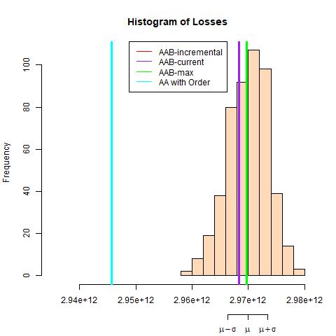
(a) Regression on Ames house prices

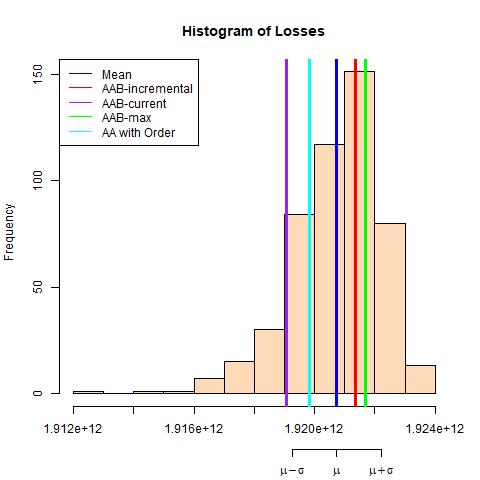
(b) RF on Ames house prices

Figure 1: Histogram of total losses

6.2.2 Comparison of AAP-incremental and AAP-max

Figure 2a illustrates the difference in total losses of AAP-incremental and AAP-max on Ames house prices data with regression models. AAP-incremental performs better at the beginning of the period when the current maximum size of the pack is much lower than the maximum pack of the whole period. After that, AAP-incremental and AAP-max have almost similar performance and the total losses level out.

Figure 2b illustrates the difference in total losses of AAP-incremental and AAP-max on Ames house prices data with RF experts. Figures 2c, 2d show the same experiment conducted on London house prices. In these cases AAP-incremental steadily outperforms AAP-max.

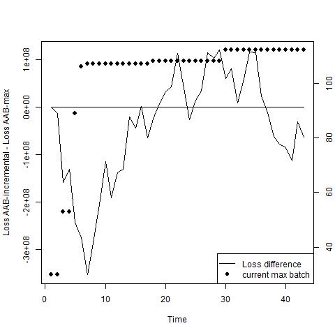
(a) Regression on Ames house prices

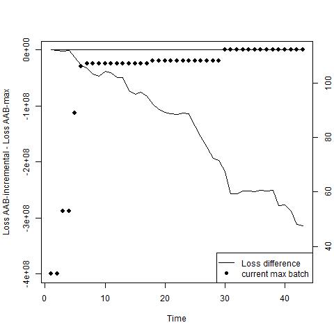
(b) RF on Ames house prices

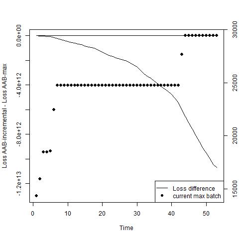
(c) Regression on London house prices

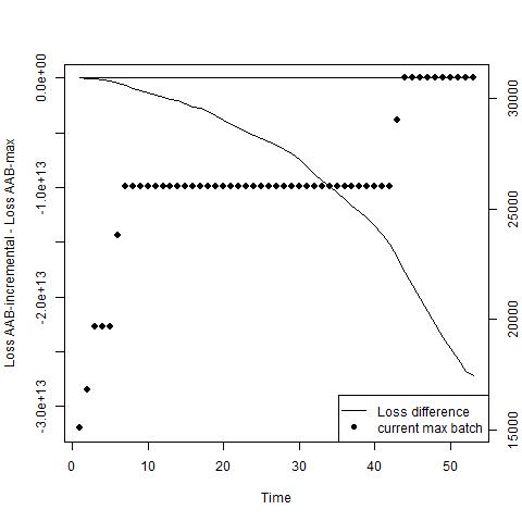
(d) RF on London house prices

Figure 2: Comparison of total losses of AAP-incremental and AAP-max

6.2.3 Comparison of AAP-current and AAP-incremental

Figure 3 illustrates the difference in total losses of AAP-current and AAP-incremental. Figures 3a and 3b show results for Ames house prices for regression and RF experts respectively, Figures 3c, 3d  — for London house prices. In all experiments AAP-current steadily outperforms AAP-incremental.

The performance of AAP-current is remarkable because by design it is not optimised to minimise the total loss. The bound of Corollary 2 is weak in comparison to that of Theorem 4. In a way, here we assess AAP-current with a measure it is not good at. Still optimal decisions of AAP-current produce superior performance.

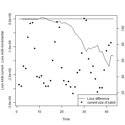
(a) Regression on Ames house prices

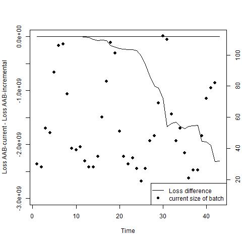
(b) RF on Ames house prices

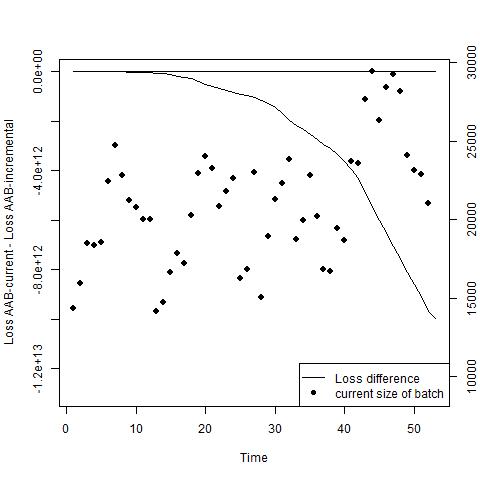
(c) Regression on London house prices

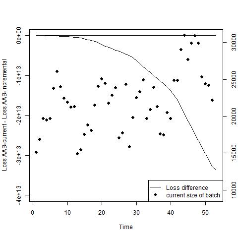
(d) RF on London house prices

Figure 3: Comparison of total losses of AAP-current and AAP-incremental

6.2.4 Comparison of AAP with Batch Models

In this section we compare AAP-incremental with two straightforward ways of prediction, which are essentially batch. One goal we have here is to do a sanity check and verify whether we are not studying properties of very bad algorithms. Secondly, we want to show that prediction with expert advice may show better ways of handling the available historical information.

In AAP we use linear regression models that have been trained on each month of the first year of the data. Is the performance of these models affected by straightforward seasonality? What if we always predicts January with the January model, February with the February model etc?

The first batch model we compare our on-line algorithm to is the seasonal model that predict January with linear regression model that has been trained on January of the first year, February — with linear model of February of the first year, etc.

In the case of ‘quarterly’ RF experts, we compete with seasonal model that predict first quarter with RF model that has been trained on the first quarter, second quarter — with RF of the second quarter, etc.

Secondly, what if we train a model on the whole of the first year? This may be more expensive than training smaller models, but what do we gain in performance? The second batch model is the linear model that has been trained on the whole first year of the data. In case of RF experts, we compete with RF model that has been trained on the first year of the data.

Figure 4 shows the comparison of total losses of AAP-current and batch linear regression models for Ames house dataset. AAP-current consistently performs better than the seasonal batch model. Thus the straightforward utilisation of seasonality does not help.

When compared to the linear regression model of the first year, AAP-current initially has higher losses but it becomes better towards the end. It could be explained as follows. AAP-current needs time to train until it becomes good in prediction. These results show that we can make a better use of the past data with prediction with expert advice than with models that were trained in the batch mode.

Table 1 shows total losses of algorithm (divided by $10^{12}$). AAP algorithms always outperform seasonal batch models. As compared to linear regression batch models that were built on the first year of the data, AAP is slightly better on Ames house dataset and slightly worse on London house dataset. RF batch models that were built on the first year of the datasets constantly outperform AAP algorithms.

The losses quoted for the parallel copies are the means over 500 random shuffles as explained above. The experiment was not run for London house prices as it is very time-consuming.

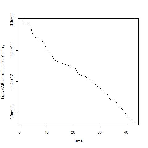
(a) Loss difference of AAP-current and
monthly batch

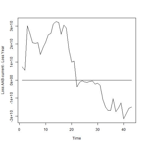
(b) Loss difference of AAP-current and
year batch

Figure 4: Comparison of total losses of AAP and batch models

Table 1: Total losses

	Ames reg	Ames RF	London reg	London RF
AAP max	2.9698	1.9217	28484.34	18819.01
AAP incremental	2.9697	1.9214	28474.26	18791.79
AAP current	2.9684	1.9191	28461.39	18758.14
Parallel copies	2.9699	1.9207	-	-
Batch Seasonal	4.6036	2.1485	28750.21	22543.43
Batch Year	2.9833	1.4699	28272.74	15877.6

6.3 Conclusion

We tested the performance of AAP against the algorithm with parallel copies of AA. We found that the average performance of algorithm with parallel copies of AA is close to the performance of AAP. AA with parallel copies ordered by PID has lower total loss than the average of AA with parallel copies which means that a meaningful ordering can have a big impact on the performance of the algorithm. In the absence of such knowledge, AAP algorithms provide more stable performance.

AAP-current is constantly outperforming AAP-incremental and AAP-max on two data sets. Therefore, we do not need to know the maximum size of the pack in advance.

Also experiments showed that in some cases we could get the better use of the past data with AAP than with models that were trained in the batch mode.

References

- [AKCV16] D. Adamskiy, W. M. Koolen, A. Chernov, and V. Vovk. A closer look at adaptive regret. The Journal of Machine Learning Research, 17(23):1–21, 2016.
- [Bel] T. Bellotti. Reliable region predictions for automated valuation models: supplementary material for Ames housing data. Available at http://wwwf.imperial.ac.uk/~abellott/publications.htm.
- [Bel17] T. Bellotti. Reliable region predictions for automated valuation models. Annals of Mathematics and Artificial Intelligence, pages 1–14, 2017.
- [CBL06] N. Cesa-Bianchi and G. Lugosi. Prediction, Learning, and Games. Cambridge University Press, 2006.
- [DC11] D. De Cock. Ames, Iowa: Alternative to the Boston housing data as an end of semester regression project. Journal of Statistics Education, 19(3), 2011.
- [JGS13] P. Joulani, A. Gyorgy, and C. Szepesvári. Online learning under delayed feedback. In Proceedings of the 30th International Conference on Machine Learning (ICML-13), pages 1453–1461, 2013.
- [KACS15] Y. Kalnishkan, D. Adamskiy, A. Chernov, and T. Scarfe. Specialist experts for prediction with side information. In 2015 IEEE International Conference on Data Mining Workshop (ICDMW), pages 1470–1477. IEEE, 2015.
- [KVV04] Y. Kalnishkan, V. Vovk, and M. V. Vyugin. Loss functions, complexities, and the Legendre transformation. Theoretical Computer Science, 313(2):195–207, 2004.
- [Loè77] M. Loève. Probability Theory I. Springer, 4th edition, 1977.
- [LW94] N. Littlestone and M. K. Warmuth. The Weighted Majority Algorithm. Information and Computation, 108:212–261, 1994.
- [QK15] K. Quanrud and D. Khashabi. Online learning with adversarial delays. In Advances in Neural Information Processing Systems, pages 1270–1278, 2015.
- [Vov90] V. Vovk. Aggregating strategies. In Proceedings of the 3rd Annual Workshop on Computational Learning Theory, pages 371–383, San Mateo, CA, 1990. Morgan Kaufmann.
- [Vov98] V. Vovk. A game of prediction with expert advice. Journal of Computer and System Sciences, 56:153–173, 1998.
- [Vov01] V. Vovk. Competitive on-line statistics. International Statistical Review, 69(2):213–248, 2001.
- [WO02] M. J. Weinberger and E. Ordentlich. On delayed prediction of individual sequences. IEEE Transactions on Information Theory, 48(7):1959–1976, 2002.
- [Zin03] M. Zinkevich. Online convex programming and generalized infinitesimal gradient ascent. In Proceedings of the 20th International Conference on Machine Learning (ICML-03), pages 928–936, 2003.