Optimum Interference Management in Underlay Inband D2D-Enhanced Cellular Networks

Abstract

For device-to-device (D2D) communications underlaying a cellular network with uplink resource sharing, both cellular and D2D links cause significant co-channel interference. In this paper, we address the critical issue of interference management in the network considering a practical path loss model incorporating both line-of-sight (LoS) and non-line-of-sight (NLoS) transmissions. To reduce the severe interference caused by active D2D links, we consider a mode selection scheme based on the maximum received signal strength (MRSS) for each user equipment (UE) to control the D2D-to-cellular interference. Specifically, a UE will operate in a cellular mode, only if its received signal strength from the strongest base station (BS) is larger than a threshold $\beta$; otherwise, the UE will operate in a D2D mode. Furthermore, we analyze the performance in terms of the coverage probability and the area spectral efficiency (ASE) for both the cellular network and the D2D one. Analytical results are obtained and the accuracy of the proposed analytical framework is validated through Monte Carol simulations. Through our theoretical and numerical analyses, we quantify the performance gains brought by D2D communications in cellular networks and we find an optimum mode selection threshold $\beta$ to maximize the total ASE in the network.

I Introduction

In the last decade, there has been a sharp increase in the demand for data traffic [1]. To address such massive consumer demand for data communications, especially from the powerful user equipment (UEs) such as smartphones and tablets, several noteworthy technologies have been proposed [2], such as small cell networks (SCNs), cognitive radio, device-to-device (D2D) communications, etc. In particular, D2D communications allow direct data transfer between a pair of neighboring mobile UEs. Due to the short communication distance between such pairs of D2D UEs, D2D communications hold great promise in improving network performance such as coverage, spectral efficiency, energy efficiency and so on [3].

In the standardization of the 5-th generation (5G) networks, the orthogonal frequency division multiple access (OFDMA) based D2D communications adopt two types of spectrum sharing methods, (i) inband (e.g., using cellular spectrum) or (ii) outband (e.g., unlicensed spectrum). In particular, in the inband D2D communications, D2D users can setup their communications in an underlay or overlay manner. More specifically, in an underlay setting, D2D users access the same spectrum of cellular users (CUs) whereas in overlay, D2D users access a dedicated portion of cellular spectrum [4]. Recently, D2D underlaying cellular networks have been standardized by the 3rd Generation Partnership Project (3GPP)[5]. For the underlay inband D2D communications, the most critical issue is to reduce the interference as cellular links and D2D links share the same radio resources.

Although the reuse of the cellular spectrum via D2D can improve the area spectral efficiency of the network, such D2D operations also pose great challenges. The major challenge in the D2D-enabled cellular network is the existence of inter-tier and intra-tier interference due to the aggressive frequency reuse, where cellular UEs and D2D UEs share the same spectrum. It is essential to design an effective interference management scheme to control the interference generated by the D2D links to the cellular links, and vice versa. Consequently, there has been a surge of academic studies in this area. Transmission power control [6, 7, 8, 9], distance based mode selection [10] and a guard zone interference control scheme [11, 12, 13] have been proposed to solve this problem. In this paper, we present a novel mode selection scheme based on the maximum received signal strength for each user equipment (UE) to control the interference. In more detail, a UE will operate in a cellular mode if its received signal strength from the strongest base station (BS) is larger than a threshold $\beta$ ; otherwise, it will operate in a D2D mode. This will mitigate large interference from the D2D links to the cellular links. To analyze the proposed interference control scheme, we develop a theoretical framework that takes power control, practical path loss and lognormal fading into account. Based on our analytical results, we find a tradeoff between the maximization of the ASE performance and the fairness of the D2D links, and the optimum setting of the threshold $\beta$ that maximizes the ASE.

Moreover, the path loss models of D2D links and cellular links in a D2D-enabled cellular network are different due to the difference in the heights and the locations of transmitters [14]. It is well known that LoS transmission may occur when the distance between a transmitter and a receiver is small, and NLOS transmission is common in office environments and in central business districts. Furthermore, when the distance between a transmitter and a receiver decreases, the probability that a LoS path exists between them increases, thereby causing a transition from NLoS transmission to LoS transmission with a higher probability. Due to the proximity between D2D users, the physical channels which constitute D2D communications are expected to be complex in nature, experiencing both LoS and NLoS conditions across these pairs, which are distinctly different from conventional cellular environments [15]. Generally speaking, D2D links are more likely to operate in LoS conditions while the cellular links are more likely to operate in NLoS conditions. To the best of our knowledge, there have been no studies that investigate network performance of D2D enhanced cellular networks, which adopts different path loss models for the cellular links and the D2D links. Our analysis shows non-trivial difference on the network performance when considering different path loss models for the cellular links and the D2D links respectively, which captures the different environment conditions that cellular links and D2D links operate in.

Compared with the existing work, the main contributions of this paper are:

• We proposed a tractable interference management scheme for each user equipment (UE) to control the co-channel interference. Specifically, a UE will operate in a cellular mode if its received signal strength from the strongest base station (BS) is larger than a threshold $\beta$ ; otherwise, it will operate in a D2D mode.

• We present a general analytical framework using stochastic geometry and intensity matching approach [16]. Then, we derive the results of coverage probability and ASE for both the cellular mode and the D2D mode UEs. Our framework considers interference management, LoS/NLoS transmission and shadow fading. The accuracy of our analytical results is validated by Monte Carlo simulations.

• Different from the existing work that does not differentiate the path loss models between cellular links and D2D links, our analysis adopts two different path loss models for cellular links and D2D links, respectively. Our results demonstrate that the D2D links can provide a considerable ASE gain when the threshold parameter is appropriately chosen. More specifically, our analysis shows the interference from D2D tier can be controlled by using our mode selection scheme, and there is an optimal $\beta$ to achieve the maximum ASE while the performance of cellular tier is guaranteed.

The rest of this paper is structured as follows. Section II provides a brief review of related work. Section III describes the system model. Section IV presents our theoretical analysis on the coverage probability and the ASE with applications in a 3GPP special case. The numerical and simulations results are discussed in Section V. Our conclusions are drawn in Section VI.

II Related Work

D2D communications underlaying cellular networks are ongoing standardization topics in LTE-A [17]. Meanwhile, stochastic geometry which is accurate in modeling irregular deployment of base stations (BSs) and mobile user equipment (UEs) has been widely used to analyze network performance [18, 19, 20]. Andrews, et.al conducted network performance analyses for the downlink (DL) [18] and the uplink (UL) [19] of SCNs, in which UEs and/or base stations (BSs) were assumed to be randomly deployed according to a homogeneous Possion point process (HPPP). In [20], Peng developed an analytical framework for the D2D communications underlaied cellular network in the DL, where a Rician fading channel model was adopted to model the small-scale fast fading for the D2D communication links. Although some studies assumed that D2D links operate on the DL spectrum, and hence the interference from BSs to D2D receivers is severe. In practice, allowing D2D links to access the UL spectrum might be a more realistic assumption, as 3GPP has standardized D2D communications [21].

On the other hand, as one of the fundamental performance metrics of the communication system, D2D transmission capacity has been analyzed in the literature [11, 6, 7, 10, 12, 13]. In [11], the author proposed an interference-limited area control scheme to mitigate the interference from cellular to D2D considering a single slope path loss model. In [9], Lee proposed a power control algorithm to control the co-channel interference in which global channel state information are required at BSs. In [10], Liu provided a unified framework to analyze the downlink outage probability in a multi-channel environment with Rayleigh fading, where D2D UEs were selected based on the average received signal strength from the nearest BS, which is equivalent to a distance-based selection. The authors of [12] and [13] proposed novel approaches to model the interference in uplink or downlink underlaid/overlaid with Rayleigh fading and single path loss model.

Meanwhile, limited studies have been conducted to consider D2D networks with general fading channels, for example in [15] and [20], the authors considered generalized fading conditions and analyzed the network performance, while they did not differentiate the path loss models between the D2D links and cellular links.

Although the existing works have provided precious insights into resource allocation and capacity enhancement for D2D communications, there are several remaining problems:

• The mode selection schemes in the literatures were not very practical, they were mostly based on the UE-to-BS distance while a more practical one which based on the maximum received signal strength should be considered.

• In some studies, only a single BS with one cellular UE and one D2D pair were considered, which did not take into account the influence from other cells. Moreover, in most studies, the authors considered D2D receiver UEs as an additional tier of nodes, independent of the cellular UEs and the D2D transmitter UEs. Such tier of D2D receiver UEs without cellular capabilities appears from nowhere and is hard to justify in practice.

• The path loss model is not practical, e.g., the impact of LoS/NLoS conditions have not been well studied in the context of D2D and usually the same path loss model was used for both the cellular and the D2D tiers. In addition, shadow fading was widely ignored in the existing analyses, which did not reflect realistic networks.

To sum up, in this paper, we propose a more generalized framework which takes into account a novel interference management scheme based on the maximum received signal strength, probabilistic NLoS and LoS transmissions and lognormal shadow fading, and shed new insight on the interference management of coexistent D2D and cellular transmissions.

III System Model

In this section, we first explain the scenario of the D2D communication coexisting with cellular network. Then, we present the path loss model and the mode selection scheme.

III-A Scenario Description

We consider a D2D underlaid UL cellular network, where BSs and UEs, including cellular UL UEs and D2D UEs, are assumed to be distributed on an infinite two-dimensional plane $\mathbf{\mathit{\mathtt{\mathbb{R}}}^{2}}$. We assume that the cellular BSs are spatially distributed according to a homogeneous PPP of intensity $\lambda_{b}$ , i.e., $\varPhi_{b}=\{X_{i}\}$, where $X_{i}$ denotes the spatial locations of the $i$th BS. Moreover, the UEs are also distributed in the network region according to another independent homogeneous PPP $\varPhi_{u}$ of intensity $\lambda_{u}$.

III-B Path Loss Model

We incorporate both NLoS and LoS transmissions into the path loss model. Following [22, 14], we adopt a very general path loss model, in which the path loss $\zeta\left(r\right)$, as a function of the distance $r$, is segmented into $N$ pieces written as

$$\zeta\left(r\right)=\begin{cases}\zeta_{1}\left(r\right),&\textrm{when }0\leq r\leq d_{1}\\ \zeta_{2}\left(r\right),&\textrm{when }d_{1}<r\leq d_{2}\\ \vdots&\vdots\\ \zeta_{N}\left(r\right),&\textrm{when }r>d_{N-1}\end{cases},$$ (1)

where each piece $\zeta_{n}\left(r\right),n\in\left\{1,2,\ldots,N\right\}$ is modeled as

$$\zeta_{n}\left(r\right)=\begin{cases}\begin{array}[]{l}\zeta_{n}^{\textrm{L}}\left(r\right)=A_{n}^{{\rm{L}}}r^{-\alpha_{n}^{{\rm{L}}}},\\ \zeta_{n}^{\textrm{NL}}\left(r\right)=A_{n}^{{\rm{NL}}}r^{-\alpha_{n}^{{\rm{NL}}}},\end{array}&\begin{array}[]{l}\textrm{LoS Probability:}\leavevmode\nobreak\ \textrm{Pr}_{n}^{\textrm{L}}\left(r\right)\\ \textrm{NLoS Probability:}\leavevmode\nobreak\ 1-\textrm{Pr}_{n}^{\textrm{L}}\left(r\right)\end{array},\end{cases}$$ (2)

where

• $\zeta_{n}^{\textrm{L}}\left(r\right)$ and $\zeta_{n}^{\textrm{NL}}\left(r\right),n\in\left\{1,2,\ldots,N\right\}$ are the $n$-th piece path loss functions for the LoS transmission and the NLoS transmission, respectively,

• $A_{n}^{{\rm{L}}}$ and $A_{n}^{{\rm{NL}}}$ are the path losses at a reference distance $r=1$ for the LoS and the NLoS cases, respectively,

• $\alpha_{n}^{{\rm{L}}}$ and $\alpha_{n}^{{\rm{NL}}}$ are the path loss exponents for the LoS and the NLoS cases, respectively.

In practice, $A_{n}^{{\rm{L}}}$, $A_{n}^{{\rm{NL}}}$, $\alpha_{n}^{{\rm{L}}}$ and $\alpha_{n}^{{\rm{NL}}}$ are constants obtainable from field tests and continuity constraints [23].

As a special case, we consider a path loss function adopted in the 3GPP [17], and we adopt two different path loss models for cellular links and D2D links as

$$\zeta_{B}\left(r\right)=\begin{cases}\begin{array}[]{l}A_{B}^{{\rm{L}}}r^{-\alpha_{B}^{{\rm{L}}}},\\ A_{B}^{{\rm{NL}}}r^{-\alpha_{B}^{{\rm{NL}}}},\end{array}&\begin{array}[]{l}\textrm{LoS Probability:}\leavevmode\nobreak\ \textrm{Pr}_{B}^{\textrm{L}}\left(r\right)\\ \textrm{NLoS Probability:}\leavevmode\nobreak\ 1-\textrm{Pr}_{B}^{\textrm{L}}\left(r\right)\end{array},\end{cases}$$ (3)

and

$$\zeta_{D}\left(r\right)=\begin{cases}\begin{array}[]{l}A_{D}^{{\rm{L}}}r^{-\alpha_{D}^{{\rm{L}}}},\\ A_{D}^{{\rm{NL}}}r^{-\alpha_{D}^{{\rm{NL}}}},\end{array}&\begin{array}[]{l}\textrm{LoS Probability:}\leavevmode\nobreak\ \textrm{Pr}_{D}^{\textrm{L}}\left(r\right)\\ \textrm{NLoS Probability:}\leavevmode\nobreak\ 1-\textrm{Pr}_{D}^{\textrm{L}}\left(r\right)\end{array},\end{cases}$$ (4)

together with a linear LoS probability function as follows [17],

$$\textrm{Pr}_{B}^{\textrm{L}}\left(r\right)=\begin{cases}1-\frac{r}{d_{B}}&0<r\leq d_{B}\\ 0&r>d_{B}\end{cases},$$ (5)

and

$$\textrm{Pr}_{D}^{\textrm{L}}\left(r\right)=\begin{cases}1-\frac{r}{d_{D}}&0<r\leq d_{D}\\ 0&r>d_{D}\end{cases},$$ (6)

where $d_{B}$ and $d_{D}$ is the cut-off distance of the LoS link for UE-to-BS links and UE-to-UE links. The adopted linear LoS probability function is very useful because it can include other LoS probability functions as its special cases [14].

III-C User Mode Selection Scheme

There are two modes for UEs in the considered D2D-enabled UL cellular network, i.e., cellular mode and D2D mode. Each UE is assigned with an operation mode according to the comparison of the maximum received DL power from its serving BS with a threshold. In more detail, the considered user model selection criterion is formulated as

$$Mode=\begin{cases}\textrm{Cellular},&\textrm{if }P^{\ast}=\underset{b}{\max}\left\{P_{b}^{\textrm{rx}}\right\}>\beta\\ \textrm{D2D},&\textrm{otherwise}\end{cases},$$ (7)

where the string variable $Mode$ takes the value of ’Cellular’ or ’D2D’ to denote the cellular mode and the D2D mode, respectively. In particular, for a tagged UE, if $P^{\ast}$ is large than a specific threshold $\beta>0$. This UE is not appropriate to work in the D2D mode due to its potentially large interference to cellular UEs. Hence, it should operate in the cellular mode and directly connect with the strongest BS; otherwise, it should operate in the D2D mode. The UEs Which are associated with cellular BSs are referred to as cellular UEs (CUs). The distance from a CU to its associated BS is denoted by $R_{B}$. From [7], we assume CUs are distributed following a non-homogenous PPP $\varPhi_{c}$. For a D2D UE, we adopt the same assumption in [10] that it randomly decides to be a D2D transmitter or a D2D receiver with equal probability at the beginning of each time slot, and a D2D receiver UE selects the strongest D2D transmitter UE for signal reception.

The received power for a typical UE from a BS $b$ can be written as

$$P_{b}^{\textrm{rx}}=\begin{cases}A_{BL}P_{B}\mathrm{\mathcal{H}_{B}}\left(b\right)R_{B}^{-\alpha_{BL}}&\mathtt{\text{LoS}}\\ A_{BN}P_{B}\mathrm{\mathcal{H}_{B}}\left(b\right)R_{B}^{-\alpha_{BN}}&\textrm{otherwise}\end{cases},$$ (8)

where $A_{BL}=10^{\frac{1}{10}A_{BL}^{\textrm{dB}}}$ and $A_{BN}=10^{\frac{1}{10}A_{BN}^{\textrm{dB}}}$ denote a constant determined by the transmission frequency for BS-to-UE links in LoS and NLoS conditions, respectively. $P_{B}$ is the transmission power of a BS, $\mathrm{\mathcal{H}_{B}}\left(b\right)$ is the lognormal shadowing from a BS $b$ to the typical UE. $\alpha_{BL}$ and $\alpha_{BN}$ denote the path loss exponents for BS-to-UE links with LoS and NLoS, respectively. Base on the above system model, we can obtain the intensity of CU as $\lambda_{c}=q\lambda_{u}$, where $q$ denotes the probability of $P^{\ast}>\beta$ and will be derived in closed-form expressions in Section IV. It is apparent that the D2D UEs are distributed following another non-homogenous PPP $\varPhi_{d}$, the intensity of which is $\lambda_{d}=\left(1-q\right)\lambda_{u}$. Considering that a required content file might not exist in a D2D transmitter, in reality, we assume that $\rho\%$ D2D transmitters possess the required content files and deliver them to D2D receivers. In other words, $\rho\%$ of the D2D links will eventually work in one time slot.

We assume an underlaid D2D model. That is, each D2D transmitter reuses the frequency with cellular UEs, which incurs inter-tier interference from D2D to cellular. However, there is no intra-cell interference between cellular UEs since we assume an orthogonal multiple access technique in a BS. It follows that there is only one uplink transmitter in each cellular BS. Here, we consider a fully loaded network with $\lambda_{u}\gg\lambda_{b}$, so that on each time-frequency resource block, each BS has at least one active UE to serve in its coverage area. Note that the case of $\lambda_{u}<\lambda_{b}$ is not trivial, which even changes the capacity scaling law [24]. In this paper, we focus on the former case, and leave the study of $\lambda_{u}<\lambda_{b}$ as our future work. Generally speaking, the active CUs can be treated as a thinning PPP $\varPhi_{c}$ with the same intensity $\lambda_{b}$ as the cellular BSs.

Moreover, we assume a channel inversion strategy for the power control for cellular UEs, i.e.,

$$P_{c_{i}}=\begin{cases}P_{0}\mathcal{\mathrm{\left(\frac{R_{i}^{\alpha_{BL}}}{\mathcal{H_{\mathrm{c_{i}}}}A_{BL}}\right)^{\varepsilon}}}&\mathtt{\text{LoS}}\\ P_{0}\mathcal{\mathrm{\left(\frac{R_{i}^{\alpha_{BN}}}{\mathcal{H_{\mathrm{c_{i}}}}A_{BN}}\right)^{\varepsilon}}}&\text{otherwise}\end{cases},$$ (9)

where $P_{c_{i}}$ is the transmission power of the $i$-th UE in cellular link, $R_{i}$ is the distance of the $i$-th link from a CU to the target BS, $\mathcal{H_{\mathrm{c_{i}}}}$ is the lognormal shadowing between target BS and the cellular UE, $\epsilon\in(0,1]$ is the fractional path loss compensation, $P_{0}$ is the receiver sensitivity. For downlink BS and D2D transmitters, they use constant transmit powers $P_{B}$ and $P_{d}$, respectively. Besides, we denote the additive white Gaussian noise (AWGN) power by $\sigma^{2}$.

III-D Performance Metrics

According to [18], the coverage probability is defined as

$$P_{Mode}\left(\gamma,\lambda_{u},\alpha_{B,D}\right)=\Pr\left[\textrm{SINR}>\gamma\right],$$ (10)

where $\gamma$ is the SINR threshold, the subscript string variable $Mode$ takes the value of ’Cellular’ or ’D2D’, and the interference in this paper consist of the interference from both cellular UEs and D2D transmitters.

Furthermore, the area spectral efficiency (ASE) in bps/Hz/k$m^{2}$ can be formulated as

$$A_{Mode}^{\textrm{ASE}}\left(\lambda_{Mode},\gamma_{0}\right)$$ (11)

$$=\lambda_{Mode}\int_{\gamma_{0}}^{\infty}\log_{2}\left(1+x\right)f_{X}\left(\lambda_{Mode},\gamma_{0}\right)dx,$$

where $\gamma_{0}$ is the minimum working SINR for the considered network, and $f_{X}\left(\lambda_{Mode},\gamma_{0}\right)$ is the PDF of the SINR observed at the typical receiver for a particular value of $\lambda_{Mode}$.

For the whole network consisting of both cellular UEs and D2D UEs, the sum ASE can be written as

$$A^{\textrm{ASE}}=A_{\textrm{Cellular}}^{\textrm{ASE}}+A_{\textrm{D2D}}^{\textrm{ASE}}.$$ (12)

IV Main Results

In this section, the performance of UEs are characterized in terms of their coverage probability and ASE both for cellular tier and D2D tier. The probability that the UE operates in the cellular mode is derived in Section IV-B, the coverage probability of cellular UE and D2D UE are derived in Section IV-B1 and Section IV-B2, respectively.

IV-A Probability operating in the cellular mode

Due to consideration of lognormal shadowing in this mode we use the intensity measure method in[16] to first obtain an equivalent network for further analysis. In particular, we transform the original PPP with lognormal shadowing to a equivalent PPP which has the matched intensity measure and intensity. More specifically, define $\overline{R}_{i}^{BL}=\mathrm{\mathcal{H}_{B}^{-1/\alpha_{BL}}}R_{i}^{BL}$ and $\overline{R}_{i}^{BN}=\mathrm{\mathcal{H}_{B}^{-1/\alpha_{BN}}}R_{i}^{BN}$, where $R_{i}^{BL}$ and $R_{i}^{BN}$ are the distance separating a typical user from its tagged strongest base station with LoS and NLoS. $\overline{R}_{i}^{BL}$ and $\overline{R}_{i}^{BN}$ are the equivalent distance separating a typical user from its tagged nearest base station in the new PPP.

The network consists of two non-homogeneous PPPs with intensities $\lambda p^{NL}(R_{i})$ and $\lambda p^{L}(R_{i})$, which representing the sets of NLoS and LoS links respectively. Each UE is associated with the strongest transmitter. Moreover, intensities $\lambda{}^{NL}(\cdot)$ and $\lambda{}^{L}(\cdot)$ are given by

$$\lambda{}^{NL}(t)=\frac{d}{dt}\varLambda^{NL}\left(\left[0,t\right]\right)$$ (13)

and

$$\lambda{}^{L}(t)=\frac{d}{dt}\varLambda^{L}\left(\left[0,t\right]\right)$$ (14)

respectively, where

$$\varLambda^{NL}\left(\left[0,t\right]\right)=\mathbb{E}_{\mathcal{H}}\left[2\pi\lambda\int_{0}^{t\left(\mathcal{H}\right)^{1/\alpha^{NL}}}p^{NL}(r)rdr\right]$$ (15)

and

$$\varLambda^{L}\left(\left[0,t\right]\right)=\mathbb{E}_{\mathcal{H}}\left[2\pi\lambda\int_{0}^{t\left(\mathcal{H}\right)^{1/\alpha^{L}}}p^{L}(r)rdr\right].$$ (16)

Similar definition are adopted to D2D tier as well. The transformed network has the exactly same performance for the typical receiver (BS or D2D RU) on the coverage probability with the original network.

In this subsection, we present our results on the probability that the UE operates in the cellular mode and the equivalence distance distributions in the cellular mode and D2D mode, respectively. In the following, we present our first result in Lemma 1, which will be used in the later analysis of the coverage probability.

Lemma 1.

The probability that a typical UE connects to the strongest BS and operates in the cellular mode $q$ is given by

$$q =1-\exp\left[-\mathbb{E}_{\mathcal{H}}\left[2\pi\lambda_{B}\int_{0}^{\left(\frac{P_{b}\textrm{A}_{BL}\mathcal{H}}{\beta}\right)^{1/\alpha_{BL}}}p^{L}(r)rdr\right]\right.$$

$$-\left.\mathbb{E}_{\mathcal{H}}\left[2\pi\lambda_{B}\int_{0}^{\left(\frac{P_{b}\textrm{A}_{BN}\mathcal{H}}{\beta}\right)^{1/\alpha_{BN}}}p^{NL}(r)rdr\right]\right],$$ (17)

and the probability that the UE operates in the D2D mode is $\left(1-q\right)$.

Proof:

See Appendix A.∎

Note that Eq.(17) explicitly account for the effects of shadow fading, pathloss, transmit power, spatial distribution of BSs and mode selection threshold $\beta$ . From the result, one can see that the HPPP $\phi_{u}$ can be divided into two PPPs: the PPP with intensity $q\lambda_{u}$ and the PPP with intensity $(1-q)\lambda_{u}$, which representing cellular UEs and D2D UEs, respectively. Same as in [7], We assume these two PPPs are independent.

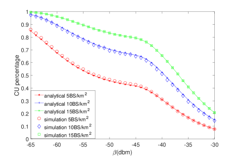
Figure 1: The probability for a UE to operate in the cellular model vary the RSS threshold $\beta$ , $\textrm{P}_{B}=46\textrm{dBm}$, log-normal shadowing with zero means, $\sigma_{B}^{2}=8\text{dB}$ and $\sigma_{D}^{2}=7\text{dB}$

Fig.1 illustrates the probability for a UE to operate in the cellular model based on Eq.(17). It can be seen that the simulation results perfectly match the analytical results. From Fig.1, we can find that over 50% UEs can operate in the cellular mode when $\beta$ is smaller than -55 dBm as the BS intensity is 5BS/k$m^{2}$. This value increases by approximately to -37 dBm and -35 dBm when the BS intensity is 10BS/k$m^{2}$ and 15BS/k$m^{2}$, respectively. It indicates that the percentage of CUs will increase as the BS intensity grows.

IV-B Coverage probability

In this subsection, we investigate the coverage probability that a receiver’s signal-to-interference-plus-noise ratio (SINR) is above a per-designated threshold $\gamma$:

$$P_{Mode}\left(T,\lambda_{u},\alpha_{B,D}\right)=\Pr\left[\textrm{SINR}>\gamma\right]$$ (18)

where $\gamma$ is the SINR threshold, the subscript string variable $Mode$ takes the value of ’Cellular’ or ’D2D’, the SINR is calculated as

$$\mathrm{SINR}=\frac{P_{Mode}\zeta_{Mode}\left(r\right)\mathcal{H_{\mathit{Mode}}}}{I_{cellular}+I_{d2d}+N_{0}},$$ (19)

where $\mathcal{H_{\mathrm{Mode}}}$ is the lognormal shadowing between transmitter and receiver in cellular mode or D2D mode. $P_{B}$, $P_{D}$ and $N_{0}$ are the transmission power of each cellular and D2D UE transmitter and the additive white Gaussian noise (AWGN) power at each receiver, respectively. $I_{cellular}$ and $I_{d2d}$ is the cumulative interference given by $I_{cellular}=\sum_{i:\,c_{i}\in\Phi_{c}\setminus signal}P_{c,i}\beta_{i}\mathcal{H}_{i},$ and $I_{d2d}=\sum_{j:\,d_{i}\in\Phi_{d2d}\setminus signal}P_{D}\beta_{j}\mathcal{H}_{j},$ where $c_{i}$ and $d_{j}$ are the $i$-th interfering CU and $j$-th interfering TU, $P_{c,i}$ is the transmit power $i$-th interfering CU, $\beta_{i}$ ,$\beta_{j}$ and $\mathcal{H_{\mathrm{i}}}$, $\mathcal{H_{\mathrm{j}}}$ are the path loss associated with $c_{i}$ and $d_{j}$, and the lognormal fading associated with $c_{i}$ and $d_{j}$, respectively.

IV-B1 Coverage probability of cellular mode

Based on the path loss model in Eq.(3,5) and the equivalence method in subsection IV-A, we present our main result on $p_{c}^{\textrm{cov}}\left(\lambda,\gamma\right)$ in Theorem 2.

Theorem 2.

For the typical BS which is located at the origin, considering the path loss model in Eq.(3) and the equivalence method, the coverage probability $p_{c}^{{\rm{cov}}}\left(\lambda,\gamma\right)$ can be derived as

$$p_{c}^{{\rm{cov}}}\left(\lambda,\gamma\right)=T_{c}^{{\rm{L}}}+T_{c}^{{\rm{NL}}},$$ (20)

where $T_{c}^{{\rm{L}}}=\int_{0}^{t_{LoS}}\left(\mathcal{\int_{\mathrm{-}\infty}^{\infty}\mathrm{\left[\frac{1-e^{-i\omega/\gamma}}{2\pi i\omega}\right]\mathcal{F}_{\frac{\textrm{1}}{SINR^{L}}}(\omega)}}d\omega\right)f_{\overline{R_{LCU}}}(r)dr$ and

$T_{c}^{{\rm{NL}}}=\int_{0}^{t_{NLoS}}\left(\mathcal{\int_{\mathrm{-}\infty}^{\infty}\mathrm{\left[\frac{1-e^{-i\omega/\gamma}}{2\pi i\omega}\right]\mathcal{F}_{\frac{\textrm{1}}{SINR^{NL}}}(\omega)}}d\omega\right)f_{\overline{R_{NLCU}}}(r)dr$ ,

$t_{LoS}=\left(\frac{\beta}{\textrm{$P_{B}A^{L}$}}\right){}^{-1/\alpha_{BL}}$,$t_{NLoS}=\left(\frac{\beta}{\textrm{$P_{B}A^{NL}$}}\right){}^{-1/\alpha_{BN}}$,

$f_{\overline{R_{LCU}}}(r)$ and $f_{\overline{R_{NLCU}}}(r)$ , are represented by

$$f_{\overline{R_{LCU}}}^{{\rm{L}}}\left(r\right)=\frac{\exp\left(-\int_{0}^{\overline{r_{1}}}\left({\rm{Pr}}^{{\rm{NL}}}\left(u\right)\right)\lambda_{B}^{NL}(u)du\right)\exp\left(-\int_{0}^{r}{\rm{Pr}}^{{\rm{L}}}\left(u\right)\lambda_{B}^{L}(u)du\right){\rm{Pr}}^{{\rm{L}}}\left(r\right)\lambda_{B}^{L}(r)}{q},$$ (21)

and

$$f_{\overline{R_{NLCU}}}^{{\rm{NL}}}\left(r\right)=\frac{\exp\left(-\int_{0}^{\overline{r_{2}}}{\rm{Pr}}^{{\rm{L}}}\left(u\right)\lambda(u)du\right)\exp\left(-\int_{0}^{r}\left({\rm{Pr}}^{{\rm{NL}}}\left(u\right)\right)\lambda_{B}^{NL}(u)du\right){\rm{Pr}}^{{\rm{NL}}}\left(r\right)\lambda_{B}^{NL}(r)}{q},$$ (22)

where $\overline{r_{1}}$ and $\overline{r_{2}}$ are given implicitly by the following equations as

$$\overline{r_{1}}=\underset{\overline{r_{1}}}{\arg}\left\{\zeta^{{\rm{NL}}}\left(\overline{r_{1}}\right)=\zeta_{n}^{{\rm{L}}}\left(\overline{r}\right)\right\},$$ (23)

and

$$\overline{r_{2}}=\underset{\overline{r_{2}}}{\arg}\left\{\zeta^{{\rm{L}}}\left(\overline{r_{2}}\right)=\zeta_{n}^{{\rm{NL}}}\left(\overline{r}\right)\right\}.$$ (24)

In addition, $\mathcal{F}_{\frac{\textrm{1}}{SINR^{L}}}(\omega)$ and $\mathcal{F}_{\frac{\textrm{1}}{SINR^{NL}}}(\omega)$ are respectively computed by

$$\mathcal{F}_{\frac{\textrm{1}}{SINR^{L}}}(\omega) =\exp\left(-\int_{r}^{\infty}\left(1-\int_{0}^{t_{LoS}}\left[\exp\left(\mathrm{i\omega\frac{\mathrm{\left(z^{\alpha_{BL}}\right)^{\varepsilon}}v^{-\alpha_{BL}}}{A_{BL}^{2\epsilon}\left(r^{-\alpha^{BL}}\right)^{1-\varepsilon}}}\right)\right]f_{\overline{R_{LCU}}}(z)dz\right)\lambda_{B}^{L}(v)dv\right)$$

$$\times \exp\left(-\int_{r}^{\infty}\left(1-\int_{0}^{t_{LoS}}\left[\exp\left(\mathrm{i\omega\frac{\mathcal{\mathrm{\left(\frac{z^{\alpha_{BL}}}{A_{BL}}\right)^{\varepsilon}}}A_{BN}v^{-\alpha_{BN}}}{\left(A_{BL}r^{-\alpha^{BL}}\right)^{1-\varepsilon}}}\right)\right]f_{\overline{R_{LCU}}}(z)dz\right)\lambda_{B}^{NL}(v)dv\right)$$

$$\times \exp\left(-\int_{t_{LoS}}^{\infty}\left(1-\exp\left(\mathrm{\mathrm{i\omega\frac{P_{d}A_{BL}v^{-\alpha_{BL}}}{P_{0}\left(A_{BL}r^{-\alpha^{BL}}\right)^{1-\varepsilon}}}}\right)\right)\lambda_{tu}^{L}(v)dv\right)$$

$$\times \exp\left(-\int_{t_{LoS}}^{\infty}\left(1-\exp\left(\mathrm{i\omega\frac{P_{d}A_{BN}v^{-\alpha_{BN}}}{P_{0}\left(A_{BL}r^{-\alpha^{BL}}\right)^{1-\varepsilon}}}\right)\right)\lambda_{tu}^{NL}(v)dv\right)$$

$$\times \exp\left(\mathrm{i\omega\frac{\sigma_{c}^{2}}{P_{0}\left(A_{BL}r^{-\alpha^{BL}}\right)^{1-\varepsilon}}}\right),$$ (25)

and

$$\mathcal{F}_{\frac{\textrm{1}}{SINR^{NL}}}(\omega) =\exp\left(-\int_{r}^{\infty}\left(1-\int_{0}^{t_{NLoS}}\left[\exp\left(\mathrm{i\omega\frac{\mathrm{\left(\frac{z^{\alpha_{BL}}}{A_{BL}}\right)^{\varepsilon}}A_{BL}v^{-\alpha_{BL}}}{\left(A_{BN}r^{-\alpha^{BN}}\right)^{1-\varepsilon}}}\right)\right]f_{\overline{R_{NLCU}}}(z)dz\right)\lambda_{B}^{L}(v)dv\right)$$

$$\times \exp\left(-\int_{r}^{\infty}\left(1-\int_{0}^{t_{NLoS}}\left[\exp\left(\mathrm{i\omega\frac{\mathrm{\left(\frac{z^{\alpha_{BL}}}{A_{BL}}\right)^{\varepsilon}}A_{BN}v^{-\alpha_{BN}}}{\left(A_{BN}r^{-\alpha^{BN}}\right)^{1-\varepsilon}}}\right)\right]f_{\overline{R_{NLCU}}}(z)dz\right)\lambda_{B}^{NL}(v)dv\right)$$

$$\times \exp\left(-\int_{t_{NLoS}}^{\infty}\left(1-\exp\left(\mathrm{\mathrm{i\omega\frac{P_{d}A_{BL}v^{-\alpha_{BL}}}{P_{0}\left(A_{BN}r^{-\alpha^{BN}}\right)^{1-\varepsilon}}}}\right)\right)\lambda_{tu}^{L}(v)dv\right)$$

$$\times \exp\left(-\int_{t_{NLoS}}^{\infty}\left(1-\exp\left(\mathrm{i\omega\frac{P_{d}A_{BN}v^{-\alpha_{BN}}}{P_{0}\left(A_{BN}r^{-\alpha^{BN}}\right)^{1-\varepsilon}}}\right)\right)\lambda_{tu}^{NL}(v)dv\right)$$

$$\times \exp\left(\mathrm{i\omega\frac{\sigma_{c}^{2}}{P_{0}\left(A_{BN}r^{-\alpha^{BN}}\right)^{1-\varepsilon}}}\right)$$ (26)

Proof:

See Appendix B. ∎

From [14], $T_{c}^{{\rm{L}}}$ and $T_{c}^{{\rm{NL}}}$ are independent of each other. The coverage probability evaluated by Eq.(20) is at least a 4-fold integral which is complicated for numerical computation. However, it gives general results that can be applied to various multi-path fading or shadowing model, e.g., Rayleigh fading, Nakagami-m fading, etc, and various NLoS/LoS transmission models as well.

The third and forth row in Eq.(25) and Eq.(26) are the aggregate interference from D2D tier. When the mode selection threshold $\beta$ increases, we can find the intensity of D2D transmitter also increases. This will reduce the coverage probability performance of cellular tier, so we make $p_{c}^{{\rm{cov}}}>\varepsilon$ as a condition to guarantee the performance for cellular mode when choosing $\beta$.

IV-B2 Coverage probability of the typical UE in the D2D mode

From [10], one can see that in order to derive the coverage probability of a generic D2D UE, we only need to derive the coverage probability for a typical D2D receiver UE. Similar to the analysis in subsection IV-B1, we focus on a typical D2D UE which is located at the origin $o$ and scheduled to receive data from another D2D UE. Following Slivnyak’s theorem for PPP, the coverage probability result derived for the typical D2D UE holds also for any generic D2D UE located at any location. In the following, we present the coverage probability for a typical D2D UE in Theorem 3.

Theorem 3.

We focus on a typical D2D UE which is located at the origin $o$ and scheduled to receive data from another D2D UE, the probability of coverage $p_{D2D}^{{\rm{cov}}}\left(\lambda,\gamma\right)$ can be derived as

$$p_{D2D}^{{\rm{cov}}}\left(\lambda,\gamma\right)=T_{D2D}^{{\rm{L}}}+T_{D2D}^{{\rm{NL}}},$$ (27)

where $T_{D2D}^{{\rm{L}}}=\int_{0}^{\infty}\left(\mathcal{\int_{\mathrm{-}\infty}^{\infty}\mathrm{\left[\frac{1-e^{-i\omega/\gamma}}{2\pi i\omega}\right]\mathcal{F}_{\frac{\textrm{1}}{SINR_{D2D}^{L}}}(\omega)}}d\omega\right)f_{\overline{R_{LD2D}}}(\overline{R_{d,0}})d\overline{R_{d,0}}$,

$T_{D2D}^{{\rm{NL}}}=\int_{0}^{\infty}\left(\mathcal{\int_{\mathrm{-}\infty}^{\infty}\mathrm{\left[\frac{1-e^{-i\omega/\gamma}}{2\pi i\omega}\right]\mathcal{F}_{\frac{\textrm{1}}{SINR_{D2D}^{NL}}}(\omega)}}d\omega\right)f_{\overline{R_{NLD2D}}}(\overline{R_{d,0}})d\overline{R_{d,0}}$ ,
$f_{\overline{R_{LD2D}}}(r)$ and $f_{\overline{R_{NLD2D}}}(r)$ can be calculated from cumulative distribution function (CDF) of $\overline{R}_{d}^{LOS}$ and $\overline{R}_{d}^{NLOS}$ in appendix C. In addition, $\mathcal{F}_{\frac{\textrm{1}}{SINR_{D2D}^{L}}}(\omega)$ and $\mathcal{F}_{\frac{\textrm{1}}{SINR_{D2D}^{NL}}}(\omega)$ are respectively computed by

$$\mathcal{F}_{\frac{\textrm{1}}{SINR_{D2D}^{L}}}(\omega) =\exp\left(-\int_{0}^{\infty}\left(1-\int_{0}^{t_{LoS}}\left[\exp\left(\mathrm{i\omega\frac{P_{0}\mathcal{\mathrm{\left(\frac{\overline{R}_{i}^{\alpha_{BL}}}{A_{BL}}\right)^{\varepsilon}}}v^{-\alpha_{dL}}}{P_{d}(\overline{R_{d,0}})^{-\alpha_{dL}}}}\right)\right]f_{\overline{R_{LCU}}}(\overline{R}_{i})d\overline{R}_{i}\right)\lambda_{B}^{L}(v)dv\right)$$

$$\times \exp\left(-\int_{0}^{\infty}\left(1-\int_{0}^{t_{LoS}}\left[\exp\left(\mathrm{i\omega\frac{P_{0}\mathcal{\mathrm{\left(\frac{\overline{R}_{i}^{\alpha_{BL}}}{A_{BL}}\right)^{\varepsilon}}}A_{DN}v^{-\alpha_{dN}}}{P_{d}A_{DL}(\overline{R_{d,0}})^{-\alpha_{dL}}}}\right)\right]f_{\overline{R_{LCU}}}(\overline{R}_{i})d\overline{R}_{i}\right)\lambda_{B}^{NL}(v)dv\right)$$

$$\times \exp\left(-\int_{r}^{\infty}\left(1-\exp\left(\mathrm{\mathrm{i\omega\frac{v^{-\alpha_{dL}}}{(\overline{R_{d,0}})^{-\alpha_{dL}}}}}\right)\right)\lambda_{tu}^{L}(v)dv\right)$$

$$\times \exp\left(-\int_{r}^{\infty}\left(1-\exp\left(\mathrm{i\omega\frac{A_{DN}v^{-\alpha_{dN}}}{A_{DL}(\overline{R_{d,0}})^{-\alpha_{dL}}}}\right)\right)\lambda_{tu}^{NL}(v)dv\right)$$

$$\times \exp\left(\mathrm{i\omega\frac{\sigma_{d}^{2}}{P_{d}A_{DL}(\overline{R_{d,0}})^{-\alpha_{dL}}}}\right),$$ (28)

and

$$\mathcal{F}_{\frac{\textrm{1}}{SINR_{D2D}^{NL}}}(\omega) =\exp\left(-\int_{0}^{\infty}\left(1-\int_{0}^{t_{NLoS}}\left[\exp\left(\mathrm{i\omega\frac{P_{0}\mathcal{\mathrm{\left(\frac{\overline{R}_{i}^{\alpha_{BL}}}{A_{BL}}\right)^{\varepsilon}}}A_{DL}v^{-\alpha_{dL}}}{P_{d}A_{DN}(\overline{R_{d,0}})^{-\alpha_{dN}}}}\right)\right]f_{\overline{R_{NLCU}}}(\overline{R}_{i})d\overline{R}_{i}\right)\lambda_{B}^{L}(v)dv\right)$$

$$\times \exp\left(-\int_{0}^{\infty}\left(1-\int_{0}^{t_{NLoS}}\left[\exp\left(\mathrm{i\omega\frac{P_{0}\mathcal{\mathrm{\left(\frac{\overline{R}_{i}^{\alpha_{BL}}}{A_{BL}}\right)^{\varepsilon}}}v^{-\alpha_{dN}}}{P_{d}(\overline{R_{d,0}})^{-\alpha_{dN}}}}\right)\right]f_{\overline{R_{NLCU}}}(\overline{R}_{i})d\overline{R}_{i}\right)\lambda_{B}^{NL}(v)dv\right)$$

$$\times \exp\left(-\int_{r}^{\infty}\left(1-\exp\left(\mathrm{\mathrm{i\omega\frac{A_{DL}v^{-\alpha_{dL}}}{A_{DN}(\overline{R_{d,0}})^{-\alpha_{dN}}}}}\right)\right)\lambda_{tu}^{L}(v)dv\right)$$

$$\times \exp\left(-\int_{r}^{\infty}\left(1-\exp\left(\mathrm{i\omega\frac{v^{-\alpha_{dN}}}{(\overline{R_{d,0}})^{-\alpha_{dN}}}}\right)\right)\lambda_{tu}^{NL}(v)dv\right)$$

$$\times \exp\left(\mathrm{i\omega\frac{\sigma_{d}^{2}}{P_{d}A_{DN}(\overline{R_{d,0}})^{-\alpha_{dN}}}}\right),$$ (29)

where $A_{DL}=10^{\frac{1}{10}A_{DL}^{\textrm{dB}}}$ and $A_{DN}=10^{\frac{1}{10}A_{DN}^{\textrm{dB}}}$ denote a constant determined by the transmission frequency for UE-to-UE links in LoS and NLoS, respectively.

Proof:

See Appendix C. ∎

The coverage probability of D2D users is evaluated by Eq.(27). Here, we assumed that D2D users are independently distributed regard to cellular users [10], so the D2D users follow a Possion point process. Although the analytical results are complicated, it provides general results that can be applied to various multi-path fading or shadowing models in the D2D-enhanced networks.

V Simulation and Discussion

In this section, we use numerical results to validate our results and analyze the performance of the D2D-enabled UL cellular network. To this end, we present the simulation parameters, the results for the coverage probability, the results for the area spectral efficiency in Section V-A, V-B, V-C, respectively.

V-A Simulation setup

According to the 3GPP LTE specifications [25], we set the system bandwith to 10MHz, carrier frequency $f_{c}$ to 2GHz, the BS intensity to $\lambda_{B}=5\,\textrm{BSs/km}^{2}$, which results in an average inter-site distance of about 500 m. The UE intensity is chosen as $\lambda=200\,\textrm{UEs/km}^{2}$, which is a typical value in 5G [14]. The transmit power of each BS and each D2D transmitter are set to $P_{B}=46\,\textrm{dBm}$ and $P_{D}=10\,\textrm{dBm}$, respectively. Moreover, the threshold for selecting cellular mode communication is $\beta=-70\sim-30\textrm{dBm}$. The standard deviation of lognormal shadowing is $8\,\textrm{dB}$ between UEs to BSs and $7\,\textrm{dB}$ between UEs to UEs. The noise powers are set to $-95\,\textrm{dBm}$ for a UE receiver and $-114\,\textrm{dBm}$ for a BS receiver, respectively. The simulation parameters are summarized in Table I.

Table I: Simulation Parameters

Parameters	Values	Parameters	Values
$\mathtt{BW}$	10MHz	$f_{c}$	2GHz
$\lambda_{B}$	5 BSs/$km^{2}$	$\sigma_{c}^{2}$	-95 dBm
$\lambda_{u}$	200 UEs/$km^{2}$	$\sigma_{d}^{2}$	-114 dBm
$\varepsilon$	0.8	$P_{0}$	-70 dBm
$\alpha_{BL}$	2.42	$A_{BL}$	$10^{-3.08}$
$\alpha_{BN}$	4.28	$A_{BN}$	$10^{-0.27}$
$\alpha_{dL}$	2	$A_{DL}$	$10^{-3.845}$
$\alpha_{dN}$	4	$A_{DN}$	$10^{-5.578}$
$P_{b}$	46 dBm	$P_{d}$	10 dBm
$d_{B}$	0.3km	$d_{D}$	0.1km

V-B Validation of analytical results of $p^{{\rm{cov}}}\left(\lambda,\gamma\right)$

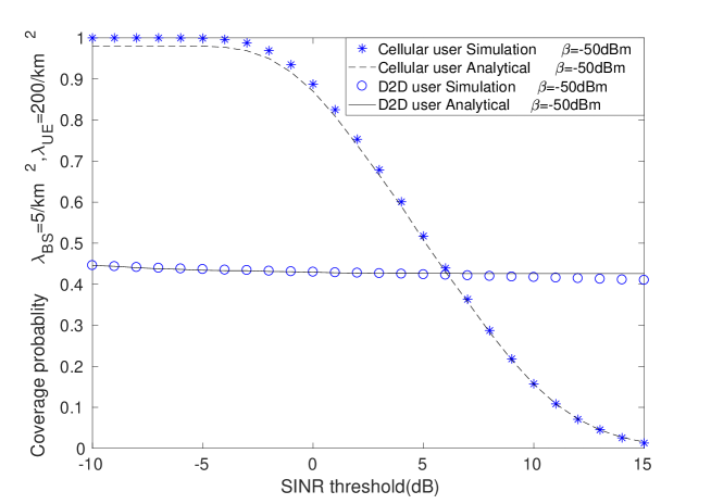
Figure 2: The Coverage Probability $p^{{\rm{cov}}}\left(\lambda,\gamma\right)$ vs. SINR threshold ($\lambda_{UE}=200\,\textrm{UEs/km}^{2}$, $\lambda_{BS}=5\,\textrm{UEs/km}^{2}$ and $\rho=10\%$). The mode select threshold $\beta$ is $-50\text{dBm}$.

In Fig. 2, we plot the results of the coverage probability of cellular tier and D2D tier, we can draw the following observations:

• The analytical results of the coverage probability from Eq.(20) and Eq.(27) match well with the simulation results, which validates our analysis and shows that the adopted model accurately captures the features of D2D communications.

• The coverage probability decreases with the increase of SINR threshold, because a higher SINR requirement makes it more difficult to satisfy the coverage criterion in Eq.(18).

• For D2D tier, the coverage probability reduces very slowly because the signals in most of the successful links are LoS while the interference is most likely NLoS, hence the SINR is relatively large, e.g., well above 15 dB.

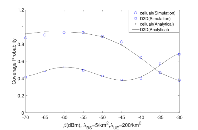
Figure 3: The Coverage Probability $p^{{\rm{cov}}}\left(\lambda,\gamma\right)$ vs. $\beta$ for 3GPP Case 1 ($\gamma_{0}=0\,\textrm{dB}$, $\lambda_{UE}=200\,\textrm{UEs/km}^{2}$, $\lambda_{BS}=5\,\textrm{UEs/km}^{2}$ and $\rho=10\%$).

To fully study the SINR coverage probability with respect to the values of $\beta$ , the results of coverage probability with various $\beta$ and $\gamma_{0}$=0 dB are plotted in Fig 3. From this figure, we can draw the following observations:

• The coverage probability of cellular users increases as $\beta$ grows from -70 dBm to -57 dBm, which is because a larger $\beta$ reduces the distance between the typical CU to the typical BS so that the signal link’s LoS probability increases. Then, the coverage probability performance decreases because the interference from D2D tier is growing. When we set $\varepsilon=0.9$, we should choose $\beta$ no larger than -45 dBm to guarantee the cellular performance.

• In the D2D mode, the coverage probability also increases as $\beta$ increases from -70 dBm to -60 dBm, this is because the distance between the typical D2D pair UEs decreases while the transmit power is constant. From $\beta=-60$ dBm to $\beta=-45$ dBm, the coverage probability decreases because the interference from the D2D tier increases. Then, the coverage probability increases when $\beta$ is larger than -45 dBm because the signal power experience the NLoS to LoS transition while the aggregate interference remains to be mostly NLoS interference.

V-C Discussion on the analytical results of ASE

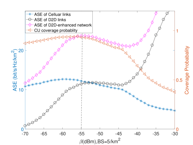
Figure 4: The ASE $A^{\textrm{ASE}}\left(\lambda,\gamma_{0}\right)$ vs. $\beta$ for 3GPP Case 1 ($\gamma_{0}=0\,\textrm{dB}$, $\lambda_{UE}=200\,\textrm{UEs/km}^{2}$, $\lambda_{BS}=5\,\textrm{UEs/km}^{2}$ and $\rho=10\%$).

The analytical results of ASE with $\gamma_{0}$=0 db vs various $\beta$ values are shown in Eq.(11). Fig.4 illustrates the ASEs of Cellular links, D2D links and of the whole network with respect to different mode selection thresholds $\beta$ . From this figure we can draw the following observations:

• The total ASE increases when $\beta\in[-55dBm,-42dBm]$, as the D2D links increases, because they do not generate a lot of interference to the cellular tier.

• An optimal $\beta$ around$-55$ dBm can achieve the maximum ASE while the coverage probability of the cellular tier is above 0.9.

• When $\beta\in[-55dBm,-42dBm]$, the total ASE decreases because the D2D links generate more interference which makes the coverage probability of cellular UEs suffer. The ASE and the coverage probability of cellular links also decrease because the aggregate interference is now mostly LoS interference.

• When $\beta\in[-42dBm,-30dBm]$, the additional D2D links make significant contribution to the ASE performance so that the total ASE grows again. Then, the total ASE approaches that of the D2D ASE because the percentage of D2D UE is approaching 100%, which has been analyzed in Eq.(17). Although the total ASE grows very quickly when $\beta\in[-42dBm,-30dBm]$, the interference from D2D links to the cellular tier remains to be large so that the performance of the cellular tier is poor. Hence, we do not recommend the network operate in this range of $\beta$.

From Fig.1 we can find D2D links will increase as $\beta$ increase for all different densities of BS. At first, D2D links will enhance the ASE performance but they do not generate a lot of interference to the cellular tier. Then the increase of D2D transmitter will generate more interference which makes the coverage probability of cellular UEs suffer. The optimal $\beta$ can be find in this stage for different densities of BS. At last the total ASE approaches to that of the D2D ASE because the percentage of D2D UE is approaching 100%. Above all, there exists an optimal $\beta$ that can achieve the maximum ASE of the D2D-enabled cellular while the coverage probability in cellular tier is guaranteed. The mode selection threshold can control the interference from both cellular tier and D2D tier. In addition, the D2D tier can nearly double the ASE for the network when appropriately choosing the threshold for mode selection.

VI Conclusion

In this paper, we proposed an interference management method in a D2D enhanced uplink cellular network, where the location of the mobile UEs and the BSs are modeled as PPPs. In particular, each UE selects its operation mode based on its downlink received power and an interference threshold $\beta$. Practical pathloss and slow shadow fading are consider in modeling the power attenuation. This mode selection method mitigates large interference from D2D transmitter to cellular network. Using a stochastic geometric approach, we analytically evaluated the coverage probability and the ASE for various values of the mode selection threshold $\beta$. Our results showed that the D2D links can provide high ASE when the threshold parameter is appropriately chosen. More importantly, we concluded that there exists an optimal $\beta$ to achieve the maximum ASE while guaranteeing the coverage probability performance of the cellular network.

As our future work, we will consider other factors of realistic networks in the theoretical analysis for SCNs, such as practical directional antennas [2] and non-HPPP deployments of BSs [26].

Appendix A:Proof of Lemma 1

Proof:

The probability that the RSS is larger than the threshold is given by

$$P=\Pr\left[\underset{b}{\max}\left\{P_{b}^{\textrm{rx}}\right\}>\beta\right],$$ (30)

where we use the standard power loss propagation model with a path loss exponent $\alpha_{BL}$ (for LoS UE-BS links) and $\alpha_{BN}$ (for NLoS UE-BS links).The probability that a generic mobile UE operates in the cellular mode is

$$q = \mathsf{\mathit{\mathrm{1}-\Pr\left[\underset{b}{\max}\left\{P_{b}^{\textrm{rx}}\right\}\leq\beta\right]}}$$ (31)

$$= 1-\Pr\left[\max\left\{P_{LOS}^{rx}\right\}\leq\beta\cap\max\left\{P_{NLOS}^{rx}\right\}\leq\beta\right]$$

$$= 1-\Pr\left[\min\overline{R}_{i}^{BL}\geq\left(\frac{P_{b}\textrm{A}_{BL}}{\beta}\right)^{1/\alpha_{BL}}\cap\min\overline{R}_{i}^{BN}\geq\left(\frac{P_{b}\textrm{A}_{BN}}{\beta}\right)^{1/\alpha_{BN}}\right]$$

$$= 1-\Pr\left[\textrm{no nodes within $\left(\frac{P_{b}\textrm{A}_{BL}}{\beta}\right)^{1/\alpha_{BL}}$}\cap\textrm{no nodes within $\left(\frac{P_{b}\textrm{A}_{BN}}{\beta}\right)^{1/\alpha_{BN}}$}\right]$$

$$= 1-\exp\left[-\wedge^{\textrm{NL}}\left(\left[0,\left(\frac{P_{b}\textrm{A}_{BL}}{\beta}\right)^{1/\alpha_{BL}}\right]\right)\right]\cdot\exp\left[-\wedge^{\textrm{L}}\left[0,\left(\frac{P_{b}\textrm{A}_{BN}}{\beta}\right)^{1/\alpha_{BN}}\right]\right]$$

$$= 1-\exp\left[-\mathbb{E}_{\mathcal{H}}\left[2\pi\lambda\int_{0}^{\left(\frac{P_{b}\textrm{A}_{BL}\mathcal{H}}{\beta}\right)^{1/\alpha_{BL}}}p^{L}(r)rdr\right]\right]$$

$$\cdot\exp\left[-\mathbb{E}_{\mathcal{H}}\left[2\pi\lambda\int_{0}^{\left(\frac{P_{b}\textrm{A}_{BN}\mathcal{H}}{\beta}\right)^{1/\alpha_{BN}}}p^{NL}(r)rdr\right]\right],$$

which concludes our proof. ∎

Appendix B:Proof of Theorem 2

Proof:

By invoking the law of total probability, the coverage probability of cellular links can be divided into two parts, i.e., $T_{c}^{{\rm{L}}}+T_{c}^{{\rm{NL}}}$, which denotes the conditional coverage probability given that the typical BS is associated with a BS in LoS and NLoS, respectively. First, we derive the coverage probability for LoS link cellular tier. Conditioned on the strongest BS being at a distance $R_{B,0}$ from the typical CU, the equivalence distance$\overline{R_{LOSCU}}=\mathrm{\mathcal{H}_{B}^{-1/\alpha_{BL}}R_{B,0}}$ $\left(\overline{R_{LOSCU}}\leq\left(\frac{\beta}{\textrm{$P_{B}A^{L}$}}\right){}^{-1/\alpha_{BL}}\right)$, probability of coverage is given by

$$T^{{\rm{L}}} =\Pr\left[\frac{1}{SINR^{L}}<\frac{1}{\gamma}\left|\textrm{LOS}\right.\right]$$

$$= \int_{0}^{t_{LoS}}\left(\int_{0}^{\frac{1}{\gamma}}f_{\frac{\textrm{1}}{SINR^{L}}}\left(x\right)dx\right)f_{\overline{R_{LCU}}}(r)dr$$

$$= \int_{0}^{t_{LoS}}\left(\int_{0}^{\frac{1}{\gamma}}\frac{1}{2\pi}\mathcal{\int_{\mathrm{-}\infty}^{\infty}F}_{\frac{\textrm{1}}{SINR^{L}}}(\omega)\cdot e^{-iwx}\cdot d\omega dx\right)f_{\overline{R_{LCU}}}(r)dr$$

$$= \int_{0}^{t_{LoS}}\left(\mathcal{\int_{\mathrm{-}\infty}^{\infty}\mathrm{\left[\frac{1-e^{-i\omega/\gamma}}{2\pi i\omega}\right]\mathcal{F}_{\frac{\textrm{1}}{SINR^{L}}}(\omega)}}d\omega\right)f_{\overline{R_{LCU}}}(r)dr\text{.}$$ (32)

where $i=\sqrt{-1}$ is the imaginary unit. The inner integral is the conditional PDF of $\frac{1}{SINR}$; The intensity of cellular UEs and D2D UEs can be calculated as

$$\lambda_{B}^{L}(t) =2\pi\lambda_{b}\frac{d}{dt}\left(\int_{0}^{\infty}\left[\int_{0}^{t\left(\mathcal{H}\right)^{1/\alpha^{L}}}\Pr^{L}(r)rdr\right]f\left(H\right)dH\right),$$ (33)

$$\lambda_{B}^{NL}(t) =\frac{d}{dt}\left(\mathbb{E}_{\mathcal{H}}\left[2\pi\lambda_{b}\int_{0}^{t\left(\mathcal{H}\right)^{1/\alpha^{NL}}}\Pr^{NL}(r)rdr\right]\right),$$ (34)

$$\lambda_{tu}^{L}(t) =\frac{d}{dt}\left(\mathbb{E}_{\mathcal{H}}\left[\pi\left(1-q\right)\lambda_{u}\int_{0}^{t\left(\mathcal{H}\right)^{1/\alpha^{L}}}\Pr^{L}(r)rdr\right]\right),$$ (35)

$$\lambda_{tu}^{NL}(t) =\frac{d}{dt}\left(\mathbb{E}_{\mathcal{H}}\left[\pi\left(1-q\right)\lambda_{u}\int_{0}^{t\left(\mathcal{H}\right)^{1/\alpha^{NL}}}\Pr^{NL}(r)rdr\right]\right),$$ (36)

$\mathcal{F}_{SINR^{-1}}(\omega)$ denotes the conditional characteristic function of $\frac{1}{SINR}$, which can be written by

$\mathcal{F}_{\frac{\textrm{1}}{SINR^{L}}}(\omega)$

$$= \int_{R^{2}}f_{\frac{\textrm{1}}{SINR^{L}}}\left(x\right)e^{i\omega x}dx$$ (37)

$$= E_{\Phi}\left[\exp\left(\mathrm{i\omega\frac{1}{SINR^{L}}}\right)\left|R_{typicalcu}=\overline{r}\right.\right]$$

$$= \mathbb{E_{\Phi}\left[\exp\left(\mathrm{i\omega\frac{I_{c}+I_{d}+\sigma^{2}}{S^{L}}}\right)\mathrm{\left|R_{typicalcu}=\overline{r}\right.}\right]}$$

$$= \mathbb{E}_{\Phi}\left[\left.\exp\left(\mathrm{i\omega\frac{I_{c}}{S^{L}}}\right)\exp\left(\mathrm{i\omega\frac{I_{d}}{S^{L}}}\right)\exp\left(\mathrm{i\omega\frac{\sigma^{2}}{S^{L}}}\right)\right|R_{typicalcu}=\overline{r}\right].$$

By applying stochastic geometry and the probability generating functional(PGFL) of the PPP. $\mathcal{F}_{\frac{\textrm{1}}{SINR^{L}}}(\omega)$ can be written as three parts, namely $\mathcal{L_{\mathrm{I_{c}}}\mathrm{(\omega)}}$,$\mathcal{L}_{\mathrm{I_{d}}}\mathrm{(\omega)}$ and $\mathcal{L_{\mathrm{n}}\mathrm{(\omega)}}$,

$$\mathcal{L}_{\mathrm{I_{c}}}\mathrm{(\omega)=} \exp\left(\mathrm{i\omega\frac{I_{CL}+I_{CN}}{S^{L}}}\right)$$

$$= \exp\left(-\int_{r}^{\infty}\left(1-\int_{0}^{t_{LoS}}\left[\exp\left(\mathrm{i\omega\frac{\mathrm{\left(z^{\alpha_{BL}}\right)^{\varepsilon}}v^{-\alpha_{BL}}}{A_{BL}^{2\epsilon}\left(r^{-\alpha^{BL}}\right)^{1-\varepsilon}}}\right)\right]f_{\overline{R_{LCU}}}(z)dz\right)\lambda_{B}^{L}(v)dv\right.$$

$$\left.-\int_{r}^{\infty}\left(1-\int_{0}^{t_{LoS}}\left[\exp\left(\mathrm{i\omega\frac{\mathcal{\mathrm{\left(z^{\alpha_{BL}}\right)^{\varepsilon}}}v^{-\alpha_{BN}}}{A_{BL}^{2\epsilon}\left(r^{-\alpha^{BL}}\right)^{1-\varepsilon}}}\right)\right]f_{\overline{R_{LCU}}}(z)dz\right)\lambda_{B}^{NL}(v)dv\right),$$ (38)

and

$$\mathcal{L}_{\mathrm{I_{d}}}\mathrm{(\omega)=} \exp\left(\mathrm{i\omega\frac{I_{DL}+I_{DN}}{S^{L}}}\right)$$

$$= \exp\left(-\int_{t_{LoS}}^{\infty}\left(1-\exp\left(\mathrm{\mathrm{i\omega\frac{P_{d}A_{BL}v^{-\alpha_{BL}}}{P_{0}\left(A_{BL}r^{-\alpha^{BL}}\right)^{1-\varepsilon}}}}\right)\right)\lambda_{tu}^{L}(v)dv\right.$$

$$\left.-\int_{t_{LoS}}^{\infty}\left(1-\exp\left(\mathrm{i\omega\frac{P_{d}A_{BN}v^{-\alpha_{BN}}}{P_{0}\left(A_{BL}r^{-\alpha^{BL}}\right)^{1-\varepsilon}}}\right)\right)\lambda_{tu}^{NL}(v)dv\right),$$ (39)

and$\mathcal{L_{\mathrm{n}}\mathrm{(\omega)}}=\exp\left(\mathrm{iw\frac{\sigma^{2}}{P_{0}\left(A_{BL}r^{-\alpha^{BL}}\right)^{1-\varepsilon}}}\right)$ which is the cellular interference , D2D interference and noise part in characteristic function.

Finally, note that the value of $p_{c}^{{\rm{cov}}}\left(\lambda,\gamma\right)$ in Eq. (20) should be calculated by taking the expectation with $f_{\overline{R_{LCU}}}(r)$ and $f_{\overline{R_{NLCU}}}(r)$, which is given as follow

$$f_{\overline{R_{LCU}}}(r) =\left(\frac{d}{dr}\left\{1-\exp\left[-\varLambda^{L}\left(\left[0,r\right]\right)\right]\cdot\exp\left[-\varLambda^{NL}\left(\left[0,\overline{r_{1}}\right]\right)\right]\right\}\left|CU\right.\right)$$

$$=\frac{\exp\left[-\varLambda^{L}\left(\left[0,r\right]\right)\right]\cdot\exp\left[-\varLambda^{NL}\left(\left[0,\overline{r_{1}}\right]\right)\right]{\rm{Pr}}^{{\rm{L}}}\left(r\right)\lambda_{B}^{L}(r)}{q},$$ (40)

where the typical UE should guarantee that there is no NLoS BS in $\overline{r_{1}}$ when the signal is LoS. Given that the typical BS is connected to a NLoS UE, the conditional coverage probability $T^{{\rm{N}}}$ can be derived in a similar way as the above. In this way, the coverage probability is obtained by $T_{c}^{{\rm{L}}}+T_{c}^{{\rm{NL}}}$. Which concludes our proof. ∎

Appendix C:Proof of Theorem 3

Proof:

The typical D2D receiver selects the equivalent nearest UE as a potential transmitter. If the potential D2D receiver is operating in a cellular mode, D2D RU must search for another transmitter. We approximately consider that the second neighbor can be found as the transmitter under this situation both for LoS/NLoS links. The approximate cumulative distribution function(CDF) of $\overline{R}_{d}^{LOS}$ can be written as

$$\Pr\left[\overline{R}_{d}^{LOS}<R\right]$$

$$\approx \int_{R+t_{LoS}}^{\infty}\left(\int_{0}^{R}f_{R_{d}^{LOS}}(\overline{R}_{d})d\overline{R}_{d}\right)f_{r_{1}^{LOS}}(r_{1})dr_{1}$$

$$+ \int_{t_{LoS}}^{R+t_{LoS}}\left(\int_{0}^{r_{1}-t_{LoS}}f_{R_{d}}(\overline{R}_{d})d\overline{R}_{d}\right.$$

$$+ \int_{r_{1}-t_{LoS}}^{R}(1-P_{c}^{L})\cdot f_{R_{d}^{LOS}}(\overline{R}_{d})d\overline{R}_{d}$$

$$+ \left.\int_{r_{1}-t_{LoS}}^{R}P_{c}^{L}\cdot f_{R_{d_{2}}^{LOS}}\left(\overline{R}_{d}\right)d\overline{R}_{d}\right)f_{r_{1}^{LOS}}(r_{1})dr_{1}$$

$$+ \int_{R+t_{NLoS}}^{\infty}\left(\int_{0}^{R}f_{R_{d}^{LOS}}(\overline{R}_{d})d\overline{R}_{d}\right)f_{r_{1}^{NLOS}}(r_{1})dr_{1}$$

$$+ \int_{t_{NLoS}}^{R+t_{NLoS}}\left(\int_{0}^{r_{1}-t}f_{R_{d}^{LOS}}(\overline{R}_{d})d\overline{R}_{d}\right.$$

$$+ \int_{r_{1}-t_{NLoS}}^{R}(1-P_{c}^{L})\cdot f_{R_{d}^{LOS}}(\overline{R}_{d})d\overline{R}_{d}$$

$$+ \left.\int_{r_{1}-t_{NLoS}}^{R}P_{c}^{L}\cdot f_{R_{d_{2}}^{LOS}}\left(\overline{R}_{d}\right)d\overline{R}_{d}\right)f_{r_{1}^{NLOS}}(r_{1})dr_{1},$$ (41)

where $r_{1}$ is the equivalent distance from TU to the strongest LoS/NLoS BS, $t_{LoS}=\left(\frac{\beta}{\textrm{$P_{B}A^{L}$}}\right){}^{-1/\alpha_{BL}}$,$t_{NLoS}=\left(\frac{\beta}{\textrm{$P_{B}A^{NL}$}}\right){}^{-1/\alpha_{BN}}$, $P_{c}^{L/NL}$is the probability of a D2D receiver be a CU.

$$f_{r_{1}^{LOS}}(r)=\frac{\exp\left[-\varLambda^{L}\left(\left[0,r\right]\right)\right]\cdot\exp\left[-\varLambda^{NL}\left(\left[0,\overline{r_{1}}\right]\right)\right]{\rm{Pr}}_{{\rm{B}}}^{{\rm{L}}}\left(r\right)\lambda_{B}^{L}(r)}{1-q}$$ (42)

and

$$f_{r_{1}^{NLOS}}(r)=\frac{\exp\left[-\varLambda^{NL}\left(\left[0,r\right]\right)\right]\cdot\exp\left[-\varLambda^{L}\left(\left[0,\overline{r_{1}}\right]\right)\right]{\rm{Pr}}_{{\rm{B}}}^{{\rm{NL}}}\left(r\right)\lambda_{B}^{NL}(r)}{1-q}$$ (43)

According to [14], if there is no difference between CUs and D2D UEs, the pdf of the distance for a tier of PPP LoS UEs is

$$f_{R_{d}^{LOS}}(r)=\exp\left(-\int_{0}^{\overline{r_{1}}}{\rm{Pr}}_{{\rm{D}}}^{{\rm{NL}}}\left(u\right)\lambda_{u}^{NL}(u)du\right)\exp\left(-\int_{0}^{r}{\rm{Pr}}_{{\rm{D}}}^{{\rm{L}}}\left(u\right)\lambda_{u}^{L}(u)du\right){\rm{Pr}}_{{\rm{D}}}^{{\rm{L}}}\left(r\right)\lambda_{u}^{L}(r)$$ (44)

and if there is no difference between CUs and D2D UEs, the pdf of the distance for a tier of PPP NLoS UEs is

$$f_{R_{d}^{NLOS}}(r)=\exp\left(-\int_{0}^{\overline{r_{2}}}{\rm{Pr}}_{{\rm{D}}}^{{\rm{L}}}\left(u\right)\lambda_{u}^{L}(u)du\right)\exp\left(-\int_{0}^{r}{\rm{Pr}}_{{\rm{D}}}^{{\rm{NL}}}\left(u\right)\lambda_{u}^{NL}(u)du\right){\rm{Pr}}_{{\rm{D}}}^{{\rm{NL}}}\left(r\right)\lambda_{u}^{NL}(r),$$ (45)

where

$$\lambda_{u}^{L}(r)=\frac{d}{dt}\left(\mathbb{E}_{\mathcal{H}}\left[2\pi\left(1-q\right)\lambda_{u}\int_{0}^{t\left(\mathcal{H}\right)^{1/\alpha^{L}}}{\rm{Pr}}_{{\rm{D}}}^{{\rm{L}}}(r)rdr\right]\right),$$ (46)

and

$$\lambda_{u}^{NL}(r)=\frac{d}{dt}\left(\mathbb{E}_{\mathcal{H}}\left[2\pi\left(1-q\right)\lambda_{u}\int_{0}^{t\left(\mathcal{H}\right)^{1/\alpha^{NL}}}{\rm{Pr}}_{{\rm{D}}}^{{\rm{NL}}}(r)rdr\right]\right),$$ (47)

According to [27] , the second neighbor point is distributed as

$$f_{R_{d_{2}}^{LOS}}(r)=2\pi^{2}r^{3}\lambda_{u}^{L}(t)^{2}\cdotp\exp\left[-\mathbb{E}_{\mathcal{H}}\left[2\pi\lambda_{u}\int_{0}^{r\left(\mathcal{H}\right)^{1/\alpha^{L}}}{\rm{Pr}}_{{\rm{D}}}^{{\rm{L}}}rdr\right]\right],$$ (48)

and

$$f_{R_{d_{2}}^{NLOS}}(r)=2\pi^{2}r^{3}\lambda_{u}^{NL}(t)^{2}\cdotp\exp\left[-\mathbb{E}_{\mathcal{H}}\left[2\pi\lambda_{u}\int_{0}^{r\left(\mathcal{H}\right)^{1/\alpha^{NL}}}{\rm{Pr}}_{{\rm{D}}}^{{\rm{NL}}}rdr\right]\right],$$ (49)

similarity, the cdf of the distance of NLoS D2D signal can be written as

$$\Pr\left[\overline{R}_{d}^{NLOS}<R\right]$$

$$\approx \int_{R+t_{LoS}}^{\infty}\left(\int_{0}^{R}f_{R_{d}^{NLOS}}(\overline{R}_{d})d\overline{R}_{d}\right)f_{r_{1}^{LOS}}(r_{1})dr_{1}$$

$$+ \int_{t_{LoS}}^{R+t_{LoS}}\left(\int_{0}^{r_{1}-t_{LoS}}f_{R_{d}^{NLOS}}(\overline{R}_{d})d\overline{R}_{d}\right.$$

$$+ \int_{r_{1}-t_{LoS}}^{R}(1-P_{c}^{NL})\cdot f_{R_{d}^{NLOS}}(\overline{R}_{d})d\overline{R}_{d}$$

$$+ \left.\int_{r_{1}-t_{LoS}}^{R}P_{c}^{NL}\cdot f_{R_{d_{2}}^{NLOS}}\left(\overline{R}_{d}\right)d\overline{R}_{d}\right)f_{r_{1}^{LOS}}(r_{1})dr_{1}$$

$$+ \int_{R+t_{NLoS}}^{\infty}\left(\int_{0}^{R}f_{R_{d}^{NLOS}}(\overline{R}_{d})d\overline{R}_{d}\right)f_{r_{1}^{NLOS}}(r_{1})dr_{1}$$

$$+ \int_{t_{NLoS}}^{R+t_{NLoS}}\left(\int_{0}^{r_{1}-t}f_{R_{d}^{NLOS}}(\overline{R}_{d})d\overline{R}_{d}\right.$$

$$+ \int_{r_{1}-t_{NLoS}}^{R}(1-P_{c}^{NL})\cdot f_{R_{d}^{NLOS}}(\overline{R}_{d})d\overline{R}_{d}$$

$$+ \left.\int_{r_{1}-t_{NLoS}}^{R}P_{c}^{NL}\cdot f_{R_{d_{2}}^{NLOS}}\left(\overline{R}_{d}\right)d\overline{R}_{d}\right)f_{r_{1}^{NLOS}}(r_{1})dr_{1},$$ (50)

the pdf of $\overline{R_{d}}^{L(NL)}$ can be written as

$$f_{\overline{R_{d}}^{L(NL)}}(r)=\frac{\partial\Pr\left[R_{d}^{L(NL)}>r\right]}{\partial\overline{R_{d}}},$$ (51)

where $P_{c}$ is the probability of the potential D2D receiver operating in the cellular mode, and it can be calculated as

$$P_{c}^{LOS/NLOS}=\arccos\left(\frac{\overline{R}_{d}+r_{1}^{2}-t_{LOS/NLOS}^{2}}{2\overline{R}_{d}r_{1}}\right)/\pi,$$ (52)

which concludes our proof. ∎

References

• [1] Cisco Visual Networking Index : Global mobile data traffic forecast update, 2015–2020 white paper. link: http://goo. gl/ylTuVx, 2016.
• [2] D. Lopez-Perez, M. Ding, H. Claussen et A. H. Jafari : Towards 1 gbps/ue in cellular systems: Understanding ultra-dense small cell deployments. IEEE Communications Surveys Tutorials, 17(4):2078–2101, Fourthquarter 2015.
• [3] J. Liu, N. Kato, J. Ma et N. Kadowaki : Device-to-device communication in lte-advanced networks: A survey. IEEE Communications Surveys Tutorials, 17(4):1923–1940, Fourthquarter 2015.
• [4] 3GPP : TR 36.828 (V11.0.0): Further enhancements to LTE Time Division Duplex (TDD) for Downlink-Uplink (DL-UL) interference management and traffic adaptation. Jun 2012.
• [5] 3GPP : TR 36.814: Further advancements for E-UTRA physical layer aspects (Release 9), Mar. 2010.
• [6] X. Lin, J. G. Andrews et A. Ghosh : Spectrum sharing for device-to-device communication in cellular networks. IEEE Transactions on Wireless Communications, 13(12):6727–6740, Dec 2014.
• [7] H. ElSawy, E. Hossain et M. S. Alouini : Analytical modeling of mode selection and power control for underlay d2d communication in cellular networks. IEEE Transactions on Communications, 62(11):4147–4161, Nov 2014.
• [8] A. Ramezani-Kebrya, M. Dong, B. Liang, G. Boudreau et S. H. Seyedmehdi : Joint power optimization for device-to-device communication in cellular networks with interference control. IEEE Transactions on Wireless Communications, 16(8):5131–5146, Aug 2017.
• [9] Namyoon Lee, Xingqin Lin, Jeffrey G Andrews et Robert W Heath : Power control for d2d underlaid cellular networks: Modeling, algorithms, and analysis. IEEE Journal on Selected Areas in Communications, 33(1):1–13, 2015.
• [10] J. Liu, H. Nishiyama, N. Kato et J. Guo : On the outage probability of device-to-device-communication-enabled multichannel cellular networks: An rss-threshold-based perspective. IEEE Journal on Selected Areas in Communications, 34(1):163–175, Jan 2016.
• [11] H. Min, J. Lee, S. Park et D. Hong : Capacity enhancement using an interference limited area for device-to-device uplink underlaying cellular networks. IEEE Transactions on Wireless Communications, 10(12):3995–4000, December 2011.
• [12] G. George, R. K. Mungara et A. Lozano : An analytical framework for device-to-device communication in cellular networks. IEEE Transactions on Wireless Communications, 14(11):6297–6310, Nov 2015.
• [13] S. Lv, C. Xing, Z. Zhang et K. Long : Guard zone based interference management for d2d-aided underlaying cellular networks. IEEE Transactions on Vehicular Technology, 66(6):5466–5471, June 2017.
• [14] M. Ding, P. Wang, D. L pez-P rez, G. Mao et Z. Lin : Performance impact of LoS and NLoS transmissions in dense cellular networks. IEEE Transactions on Wireless Communications, 15(3):2365–2380, Mar. 2016.
• [15] Y. J. Chun, S. L. Cotton, H. S. Dhillon, A. Ghrayeb et M. O. Hasna : A stochastic geometric analysis of device-to-device communications operating over generalized fading channels. IEEE Transactions on Wireless Communications, 16(7):4151–4165, July 2017.
• [16] M. Di Renzo, W. Lu et P. Guan : The intensity matching approach: A tractable stochastic geometry approximation to system-level analysis of cellular networks. IEEE Transactions on Wireless Communications, 15(9):5963–5983, Sept 2016.
• [17] 3GPP : TR 36.828: Further enhancements to LTE Time Division Duplex (TDD) for Downlink-Uplink (DL-UL) interference management and traffic adaptation, Jun. 2012.
• [18] J. G. Andrews, F. Baccelli et R. K. Ganti : A tractable approach to coverage and rate in cellular networks. IEEE Transactions on Communications, 59(11):3122–3134, November 2011.
• [19] T. D. Novlan, H. S. Dhillon et J. G. Andrews : Analytical modeling of uplink cellular networks. IEEE Transactions on Wireless Communications, 12(6):2669–2679, June 2013.
• [20] Mugen Peng, Yuan Li, Tony QS Quek et Chonggang Wang : Device-to-device underlaid cellular networks under rician fading channels. Wireless Communications, IEEE Transactions on, 13(8):4247–4259, 2014.
• [21] 3GPP : TR 36.877 (RAN4) LTE Device to Device (D2D) Proximity Services (ProSe) C UE radio transmission and reception. Mar 2015.
• [22] M. Ding, D. L pez-P rez, G. Mao, P. Wang et Z. Lin : Will the area spectral efficiency monotonically grow as small cells go dense? IEEE GLOBECOM 2015, pages 1–7, Dec. 2015.
• [23] Spatial Channel Model AHG : Subsection 3.5.3, Spatial Channel Model Text Description V6.0, Apr. 2003.
• [24] M. Ding, D. L pez-P rez et G. Mao : A new capacity scaling law in ultra-dense networks. arXiv:1704.00399 [cs.NI], Apr. 2017.
• [25] 3GPP : TR 36.872: Small cell enhancements for E-UTRA and E-UTRAN - Physical layer aspects, Dec. 2013.
• [26] M. Ding et D. L pez-P rez : On the performance of practical ultra-dense networks: The major and minor factors. In 2017 15th International Symposium on Modeling and Optimization in Mobile, Ad Hoc, and Wireless Networks (WiOpt), pages 1–8, May 2017.
• [27] M. Haenggi : On distances in uniformly random networks. IEEE Transactions on Information Theory, 51(10):3584–3586, Oct 2005.