Continuum extrapolation of critical point for finite temperature QCD with $N_{\rm f}=3$

Abstract

We study the critical point for finite temperature $N_{\rm f}=3$ QCD using several temporal lattice sizes up to 10. In the study, the Iwasaki gauge action and non-perturbatively O(a) improved Wilson fermions are employed. We estimate the critical temperature and the upper bound of the critical pseudo-scalar meson mass.

1 Introduction

It is an important issue to understand the nature of finite temperature QCD phase transition with various parameters, for example, the quark masses and the number of flavors. Such an information of the nature of the phase transition is summarized in the columbia plot (Fig.1). The heavy region is well studied for example in Ref.Saito:2011fs . On the other hand, in the chiral region, there are some qualitative predictions by the effective theory Pisarski:1983ms ; Butti:2003nu ; Calabrese:2004uk with the renormalization group analysis, but the quantitative knowledge is still lacking. Our ultimate goal is to quantitatively fix a shape of the critical line in the chiral region by using the lattice QCD simulation. See deForcrand:2006pv ; Endrodi:2007gc for previous studies on the critical line, and Nakamura for our current approach. In this article, we focus on 3-flavor symmetric case and try to identify the critical point whose location is marked by a star in Fig. 1.

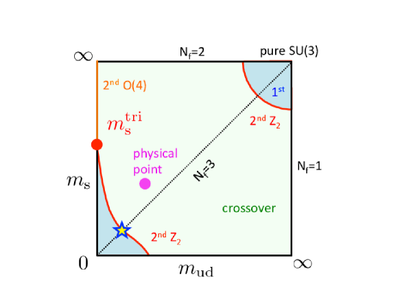
Figure 1: Columbia plot. Our aim is to fix the critical point (marked as star) on the 3-flavor symmetric line in the chiral region.

Table 1 summarizes the value of the critical peseudo-scalar meson mass for 3-flavor QCD obtained by the lattice simulations Aoki:1998gia ; Karsch:2001nf ; Liao:2001en ; Karsch:2003va ; deForcrand:2007rq ; Varnhorst:2015lea ; Bazavov:2017xul ; Iwasaki:1996zt ; Jin:2014hea ; Takeda:2016vfj ; Smith:2011pm ; Jin:2017jjp . There are many works using staggered type fermions. Those results basically show that for larger $N_{\rm t}$ and more improvement, the critical mass tends to be small. Recently the upper bound of the critical pion mass has been updated and it turns out to be very small $m_{{\rm PS,critical}}\lesssim 50$ MeV Bazavov:2017xul , and in some case it could be even zero Varnhorst:2015lea . On the other hand for Wilson type fermions, there is old study where the critical mass was shown to be very heavy Iwasaki:1996zt , but recently with the improvement of the action we obtain a relatively smaller value. In this article, we update our value of the critical mass by using larger temporal lattices Jin:2014hea ; Takeda:2016vfj . More details of the contents in this article can be found in Jin:2017jjp .

Table 1: Summary of the pseudo-scalar meson at the critical point for $N_{\rm f}=3$ QCD deForcrand:2017cgb .

Action	$N_{\rm t}$	$m_{{\rm PS,critical}}$ [MeV]	Ref.
staggered, standard	4	290	Karsch:2001nf
staggered, p4	4	67	Karsch:2003va
staggered, standard	6	150	deForcrand:2007rq
staggered, HISQ	6	$\lesssim$ 50	Bazavov:2017xul
staggered, stout	4-6	could be 0	Varnhorst:2015lea
Wilson, standard	4	$\lesssim$ 670	Iwasaki:1996zt
Wilson, NP O($a$) improved	4-8	300	Jin:2014hea ; Takeda:2016vfj
Wilson, NP O($a$) improved	4-10	$\lesssim 170$	Jin:2017jjp

2 Simulation setup

We use the Iwasaki gauge action Iwasaki:2011np and non-perturbatively O($a$) improved Wilson fermions Aoki:2005et . The temporal lattice $N_{\rm t}=4$, 6, 8 and 10 are used in our study. To carry out the finite size scaling, the spatial lattice size is varied. In order to determine the critical point we use the conventional kurtosis intersection analysis Karsch:2001nf . As an observable we use the naive chiral condensate. We measure higher order of the mass-derivatives of the quark propagator by using the noise method. They are used for the computation of the higher moments of the chiral condensate as well as for the $\kappa$-reweighting, that is, the reweighting factor which is a ratio of quark determinant is approximately computed as in Kuramashi:2016kpb . BQCD code Nakamura:2010qh and RHMC algorithm Clark:2006fx are used to generate the gauge configurations.

3 Simulation results

Typical results for the higher moments of the chiral condensate (susceptibility and kurtosis) are shown in Fig. 2 for $N_{\rm t}=10$ and $\beta=1.78$ and with some spatial volumes $N_{\rm s}=16-28$. The kappa is used as a probe parameter. In Fig. 2, $\kappa$-reweighting together with the multi-ensemble Ferrenberg:1988yz results are also shown. From the peak position of the susceptibility we determine the transition point. Figure 3 summarizes the transition line for $N_{\rm t}=4$, $6$, $8$ and $10$ in the bare parameter space spanned by $\beta$ and $\kappa$.

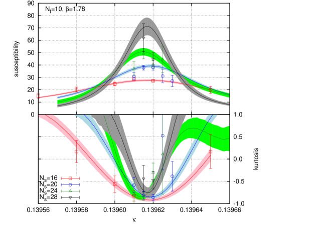
Figure 2: Susceptibility and kurtosis for the naive chiral condensate as a function of $\kappa$. Simulation parameters: $N_{\rm t}=10$, $\beta=1.78$, $N_{\rm s}=16$, $20$, $24$ and $28$. The band shows the multi-ensemble reweighting results.

Figure 3: The transition points (TP) are represented by open symbols for $N_{\rm t}=4$, 6, 8 and 10. Filled symbols on the transition line show the location of the critical end point (CEP). The critical point is determined by the kurtosis intersection by using fitting formula in eq.(1). The green curve represents the massless pion line at the zero-temperature.

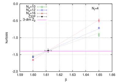
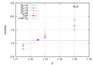
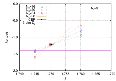
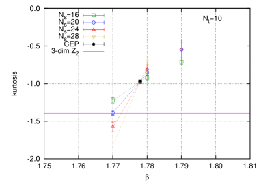
Figure 4: Kurtosis intersection for $N_{\rm t}=4$, $6$, $8$ and 10. The black point represents the intersection point. The horizontal magenta line shows the value of the kurtosis for three-dimensional Z₂ universality class.

The minimum of kurtosis along the transition line projected on the $\beta$ axis is plotted in Fig. 4. Although for smaller $N_{\rm t}$ ($=4$ and $6$) a consistency with the three-dimensional Z₂ universality class is clearly observed, for higher $N_{\rm t}$ ($=8$ and $10$) the value of kurtosis of the critical point is larger than that of the Z₂. One of possibility to explain this behavior is the finite size effects. One conceives two sources of the finite size effects:

1. Contribution of energy-like operator in the chiral condensate.

2. An effect of the leading irrelevant scaling field.

Actually they suggest a similar modified form for the kurtosis intersection analysis,

$$K=\left[K_{\rm E}+AN_{\rm s}^{1/\nu}(\beta-\beta_{\rm E})\right](1+BN_{\rm s}^{-C}),$$ (1)

where $C=C_{\rm A}=0.894$ for (A) and $C=C_{\rm B}=0.83...$ for (B) in the case of three-dimensional Z₂ universality class. Since it is hard to distinguish between them in the fitting, we fix $C=C_{\rm A}$ during the fitting procedure where $\beta_{\rm E}$, $A$ and $B$ are used as fitting parameters. The fitting results are shown in Table 2. And then we obtain a reasonable result which is consistent with the Z₂ universality class, that is, fitting assuming the value of $K_{\rm E}$ to be $-1.396$ and $\nu=0.63$ gives reasonable $\chi^{2}/{\rm d.o.f.}\sim O(1)$ for $N_{\rm t}=8$ and 10. The resulting new critical points are plotted in Fig. 3.

Table 2: Fit results for kurtosis intersection with fitting form in eq.(1). A value without error bar means that the corresponding fit parameter is fixed to the given value during the fit.

$N_{\rm t}$	Fit	$\beta_{\rm E}$	$\kappa_{\rm E}$	$K_{\rm E}$	$\nu$	$A$	$B$	$C$	$\chi^{2}/{\rm d.o.f.}$
4	$1$	$1.6115(26)$	$0.1429337(13)$	$-1.383(48)$	$0.84(13)$	$0.88(42)$	$\times$	$\times$	$1.75$
	$2$	$1.61065(61)$	$0.1429713(13)$	$-1.396$	$0.63$	$0.313(12)$	$\times$	$\times$	$3.05$
	$3$	$1.6099(17)$	$0.1430048(13)$	$-1.396$	$0.63$	$0.311(14)$	$0.10(21)$	$0.894$	$3.77$
6	$1$	$1.72518(71)$	$0.1406129(14)$	$-1.373(17)$	$0.683(54)$	$0.58(17)$	$\times$	$\times$	$0.68$
	$2$	$1.72431(24)$	$0.1406451(14)$	$-1.396$	$0.63$	$0.418(11)$	$\times$	$\times$	$0.70$
	$3$	$1.72462(40)$	$0.1406334(14)$	$-1.396$	$0.63$	$0.422(12)$	$-0.052(52)$	$0.894$	$0.70$
8	$1$	$1.75049(57)$	$0.1402234(11)$	$-1.219(25)$	$0.527(55)$	$0.146(88)$	$\times$	$\times$	$0.73$
	$2$	$1.74721(42)$	$0.14031921(76)$	$-1.396$	$0.63$	$0.404(36)$	$\times$	$\times$	$5.99$
	$3$	$1.74953(33)$	$0.1402512(10)$	$-1.396$	$0.63$	$0.414(13)$	$-1.33(15)$	$0.894$	$0.73$
10	$1$	$1.77796(48)$	$0.1396661(17)$	$-0.974(25)$	$0.466(45)$	$0.084(52)$	$\times$	$\times$	$0.22$
	$2$	$1.7694(16)$	$0.1398724(22)$	$-1.396$	$0.63$	$0.421(95)$	$\times$	$\times$	$10.03$
	$3$	$1.77545(53)$	$0.1397274(17)$	$-1.396$	$0.63$	$0.559(29)$	$-2.97(25)$	$0.894$	$0.43$

4 Continuum extrapolation of the critical point

Next step is to express the bare critical point in terms of hadronic physical quantity. For that purpose we carry out the zero temperature simulation and compute the Wilson flow scale $\sqrt{t_{0}}$ Luscher:2010iy and the pseudo-scalar meson mass $m_{\rm PS}$. The transformation of the critical point from the bare parameter space to the physical one for $N_{\rm t}=10$ is shown in Fig. 5.

The continuum extrapolation of the critical temperature $T_{\rm E}$ is shown in Fig. 6 (upper-left panel). The data points at $N_{\rm t}=6$, 8 and 10 are in a good scaling region and we obtain the continuum value (in physical units Borsanyi:2012zs )

$$T_{\rm E}=134(3)\mbox{MeV}.$$ (2)

On the other hand, for critical pion mass in Fig. 6 (upper-right and lower-left), it has a large scaling violation and the extrapolation has ambiguity, namely the extrapolation depends on fitting range and fitting form. We also check the pion mass square as in Fig.6 (lower-right). In this case, we somehow obtain a negative value. This shows that our data points may be not in the scaling region and it is hard to quote a single value for an extrapolation. Therefore, we conservatively estimate an upper bound of the critical pion mass. We take the maximum value among all fits that we did as the upper bound (in physical units),

$$m_{\rm PS,E}\lesssim 170\mbox{MeV}.$$ (3)

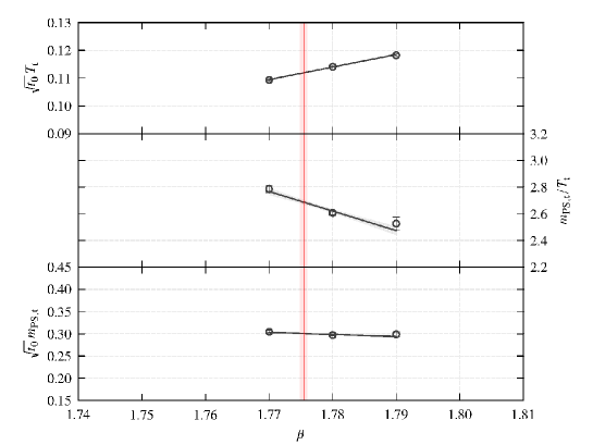
Figure 5: The transformation of the critical point from the bare parameter space to physical one. The red vertical line shows the location of the bare critical point. The black line is the interpolation of the dimensionless physical quantity along the transition line. The intersection of the red and black line gives the estimation of $\sqrt{t_{0}}T$, $m_{\rm PS}/T$ and $\sqrt{t_{0}}m_{\rm PS}$ at the critical point.

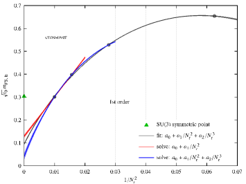
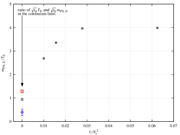
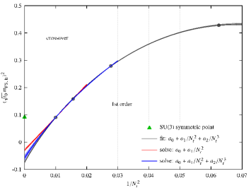
Figure 6: Continuum extrapolation of the critical temperature and the critical pseudo-scalar meson mass.

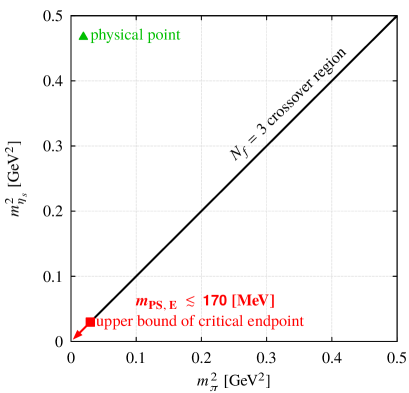
Figure 7: Summary plot (Columbia-like plot) of our result.

5 Summary and outlook

We carry out the finite temperature $N_{\rm f}=3$ QCD simulation by using non-perturvatively O($a$) improved Wilson fermions and study the critical end point by using the kurtosis intersection. By carrying out large scale simulations up to $N_{\rm t}=10$, we attempt to take the continuum limit of the critical end point. Although we stably obtain the critical temperature $T_{\rm E}=134(3)$ MeV, the critical pseudo-scalar meson mass has large ambiguity caused in the continuum extrapolation. Therefore we conservatively estimate the upper bound $m_{\rm PS,E}\lesssim 170$ MeV. A summary plot of our result is shown in Fig. 7 where both axes are represented by meson masses $m_{\pi}^{2}$ and $m_{\eta_{\rm s}}^{2}$ which may be proportional to the quark masses $m_{\rm ud}$ and $m_{\rm s}$ respectively. Our upper bound is relatively larger than that of HISQ Bazavov:2017xul , $m_{\rm PS,E}\lesssim 50$ MeV. Note that, however, our upper bound is estimated from the fact that there is critical point, while in the HISQ study the bound comes from the absence of the critical point.

In future, it is very important to fix the value of the critical end point or push down the upper bound. For Wilson type fermions, one has to handle the scaling violation. In order to take the continuum limit more smoothly and reliably one needs to run further large scale simulations say at $N_{\rm t}=12$ or implement some improvement on the lattice action or lattice setup.

References

- (1) H. Saito et al. [WHOT-QCD Collaboration], Phys. Rev. D 84, 054502 (2011) Erratum: [Phys. Rev. D 85, 079902 (2012)] [arXiv:1106.0974 [hep-lat]].
- (2) R. D. Pisarski and F. Wilczek, Phys. Rev. D 29, 338 (1984).
- (3) P. Calabrese and P. Parruccini, JHEP 0405, 018 (2004) [hep-ph/0403140].
- (4) A. Butti, A. Pelissetto and E. Vicari, JHEP 0308, 029 (2003) [hep-ph/0307036].
- (5) P. de Forcrand and O. Philipsen, JHEP 0701, 077 (2007) [hep-lat/0607017].
- (6) G. Endrodi, Z. Fodor, S. D. Katz and K. K. Szabo, PoS LAT 2007, 182 (2007) [arXiv:0710.0998 [hep-lat]].
- (7) Y. Kuramashi, Y. Nakamura and S. Takeda, Proceedings,35th International Symposium on Lattice Field Theory (Lattice2017): Granada, Spain, to appear in EPJ Web Conf.
- (8) S. Aoki et al. [JLQCD Collaboration], Nucl. Phys. Proc. Suppl. 73, 459 (1999) [hep-lat/9809102].
- (9) F. Karsch, E. Laermann and C. Schmidt, Phys. Lett. B 520, 41 (2001) [hep-lat/0107020].
- (10) X. Liao, Nucl. Phys. Proc. Suppl. 106, 426 (2002) [hep-lat/0111013].
- (11) F. Karsch, C. R. Allton, S. Ejiri, S. J. Hands, O. Kaczmarek, E. Laermann and C. Schmidt, Nucl. Phys. Proc. Suppl. 129, 614 (2004) [hep-lat/0309116].
- (12) D. Smith and C. Schmidt, PoS LATTICE 2011 (2011) 216 [arXiv:1109.6729 [hep-lat]].
- (13) P. de Forcrand, S. Kim and O. Philipsen, PoS LAT 2007, 178 (2007) [arXiv:0711.0262 [hep-lat]].
- (14) L. Varnhorst, PoS LATTICE 2014, 193 (2015).
- (15) A. Bazavov, H.-T. Ding, P. Hegde, F. Karsch, E. Laermann, S. Mukherjee, P. Petreczky and C. Schmidt, Phys. Rev. D 95, no. 7, 074505 (2017) [arXiv:1701.03548 [hep-lat]].
- (16) Y. Iwasaki, K. Kanaya, S. Kaya, S. Sakai and T. Yoshie, Phys. Rev. D 54, 7010 (1996) [hep-lat/9605030].
- (17) X. Y. Jin, Y. Kuramashi, Y. Nakamura, S. Takeda and A. Ukawa, Phys. Rev. D 91, no. 1, 014508 (2015) [arXiv:1411.7461 [hep-lat]].
- (18) S. Takeda, X. Y. Jin, Y. Kuramashi, Y. Nakamura and A. Ukawa, PoS LATTICE 2016, 384 (2017) [arXiv:1612.05371 [hep-lat]].
- (19) X. Y. Jin, Y. Kuramashi, Y. Nakamura, S. Takeda and A. Ukawa, Phys. Rev. D 96, no. 3, 034523 (2017) [arXiv:1706.01178 [hep-lat]].
- (20) P. de Forcrand and M. D’Elia, PoS LATTICE 2016, 081 (2017) [arXiv:1702.00330 [hep-lat]].
- (21) Y. Iwasaki, Report No. UTHEP-118 (1983), arXiv:1111.7054 [hep-lat].
- (22) S. Aoki et al. [CP-PACS and JLQCD Collaborations], Phys. Rev. D 73, 034501 (2006) [hep-lat/0508031].
- (23) Y. Kuramashi, Y. Nakamura, S. Takeda and A. Ukawa, Phys. Rev. D 94, no. 11, 114507 (2016) [arXiv:1605.04659 [hep-lat]].
- (24) Y. Nakamura and H. Stuben, PoS LATTICE 2010, 040 (2010) [arXiv:1011.0199 [hep-lat]].
- (25) M. A. Clark and A. D. Kennedy, Phys. Rev. Lett. 98, 051601 (2007) [hep-lat/0608015].
- (26) A. M. Ferrenberg and R. H. Swendsen, Phys. Rev. Lett. 61, 2635 (1988).
- (27) M. Lüscher, JHEP 1008, 071 (2010) Erratum: [JHEP 1403, 092 (2014)] [arXiv:1006.4518 [hep-lat]].
- (28) S. Borsanyi et al., JHEP 1209, 010 (2012) [arXiv:1203.4469 [hep-lat]].