Characterizing and Enumerating Walsh-Hadamard Transform Algorithms

Abstract

We propose a way of characterizing the algorithms computing a Walsh-Hadamard transform that consist of a sequence of arrays of butterflies ($I_{2^{n-1}}\otimes\operatorname{DFT}_{2}$) interleaved by linear permutations. Linear permutations are those that map linearly the binary representation of its element indices. We also propose a method to enumerate these algorithms.

1 Introduction

The Walsh-Hadamard transform (WHT) is an important function in signal processing [1] and coding theory [6]. It shares many properties with the Discrete Fourier Transform (DFT), including a Cooley-Tukey [2] divide-and-conquer method to derive fast algorithms. Pease-like [7] WHT (Fig 1(a)) and the iterative Cooley-Tukey WHT (Fig 1(b)) are two examples of these. The algorithms obtained with this method share the same structure: a sequence of arrays of butterflies, i.e., a block computing a DFT on $2$ elements, interleaved with linear permutations. Linear permutations are a group of permutations appearing in many signal processing algorithms, comprising the bit-reversal, the perfect shuffle, and stride permutations.

In this article, we consider the converse problem; we derive the conditions that a sequence of linear permutations has to satisfy for the corresponding algorithm to compute a WHT (Theorem 1). Additionally, we provide a method to enumerate such algorithms (Corollary 1).

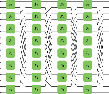
(a) Pease WHT

(b) Iterative Cooley-Tukey

Figure 1: Dataflow of two Cooley-Tukey derived fast algorithms computing a WHT on $16$ elements. The $F_{2}$ blocks represent butterflies.

1.1 Background and notation

Hadamard matrix. For a positive integer $n$, and given $x\in\mathbb{R}^{2^{n}}$, the WHT computes $y=H_{n}\cdot x$, where $H_{n}$ is the Hadamard matrix [3], the $2^{n}\times 2^{n}$ square matrix defined recursively by

$$H_{n}=\begin{cases}\operatorname{DFT}_{2},&\text{ for n=1, and}\\ \left(\begin{array}[]{rr}H_{n-1}&H_{n-1}\\ H_{n-1}&-H_{n-1}\end{array}\right),&\text{ for n>1.}\\ \end{cases}$$

Here, $\operatorname{DFT}_{2}$ is the butterfly, i.e. the matrix

$$\operatorname{DFT}_{2}=\begin{pmatrix}\begin{array}[]{rr}1&1\\ 1&-1\end{array}\end{pmatrix}.$$

For instance, the WHT on $8$ elements corresponds to the matrix

$$H_{3}=\begin{pmatrix}\begin{array}[]{rrrrrrrr}1&1&1&1&1&1&1&1\\ 1&-1&1&-1&1&-1&1&-1\\ 1&1&-1&-1&1&1&-1&-1\\ 1&-1&-1&1&1&-1&-1&1\\ 1&1&1&1&-1&-1&-1&-1\\ 1&-1&1&-1&-1&1&-1&1\\ 1&1&-1&-1&-1&-1&1&1\\ 1&-1&-1&1&-1&1&1&-1\end{array}\end{pmatrix}.$$

Binary representation. For an integer $0\leq i<2^{n}$, we denote with $i_{b}$ the column vector of $n$ bits containing the binary representation of $i$, with the most significant bit on the top ($i_{b}\in\mathbb{F}_{2}^{n}$, where $\mathbb{F}_{2}$ is the Galois field with two elements). For instance, for $n=3$, we have

$$6_{b}=\begin{pmatrix}1\\ 1\\ 0\end{pmatrix}.$$

Using this notation, a direct computation shows that the Hadamard matrix can be rewritten as

$$H_{n}=\left((-1)^{i_{b}^{T}j_{b}}\right)_{0\leq i,j<2^{n}}.$$ (1)

Cooley-Tukey Fast WHT. Cooley-Tukey algorithms are based on the following identity, satisfied by the Hadamard matrix:

$$H_{n}=H_{p}\otimes H_{q}=(H_{p}\otimes I_{2^{q}})\cdot(I_{2^{p}}\otimes H_{q})\text{, where }p+q=n.$$ (2)

Using this formula recursively – along with properties [4] of the Kronecker product $\otimes$ – yields expressions consisting of $n$ arrays of $2^{n-1}$ butterflies,

$$I_{2^{n-1}}\otimes\operatorname{DFT}_{2}=\begin{array}[]{c}\begin{pmatrix}\operatorname{DFT}_{2}&&\\ &\ddots&\\ &&\operatorname{DFT}_{2}\end{pmatrix}\\ \underbrace{\rule{78.0pt}{0.0pt}}_{2^{n-1}\text{ times}}\end{array},$$

interleaved by permutations. For instance, the Pease-like [7] algorithm for the WHT (Fig. 1(a)) uses $n$ perfect shuffles, a permutation that interleaves the first and second half of its input, and that we denote with $\pi(C_{n})$:

$$H_{n}=\prod_{k=1}^{n}\left((I_{2^{n-1}}\otimes\operatorname{DFT}_{2})\pi(C_{n})\right).$$ (3)

More generally, it is possible to enumerate all possible algorithms yielded by (2) by keeping the different values of $p$ and $q$ used in a partition tree [5]. The permutations obtained in this case are the identity, stride-permutations, and the permutations obtained by composition and Kronecker product of these. The group of linear permutations contains these [8].

Linear permutation. If $Q$ is an $n\times n$ invertible bit-matrix ($Q\in\operatorname{GL}_{n}(\mathbb{F}_{2})$), we denote with $\pi(Q)$ the associated linear permutation, i.e. the permutation on $2^{n}$ points that maps the element indexed by $0\leq i<2^{n}$ to the index $j$ satisfying $j_{b}=Qi_{b}$. As an example, the matrix

$$C_{n}=\begin{pmatrix}&1&&\\ &&\ddots&\\ &&&1\\ 1&&&\end{pmatrix},$$

rotates the bits up, and its associated linear permutation is the perfect shuffle, hence the notation we used for it, $\pi(C_{n})$.

Sequence of linear permutations. In the rest of this article, we consider a sequence of $n+1$ invertible $n\times n$ bit-matrices $P=(P_{0},P_{1},\dots,P_{n})$, and the computation

$$W(P)=\pi(P_{0})\cdot(I_{2^{n-1}}\otimes\operatorname{DFT}_{2})\cdot\pi(P_{1})\cdot(I_{2^{n-1}}\otimes\operatorname{DFT}_{2})\dots\pi(P_{n-1})\cdot(I_{2^{n-1}}\otimes\operatorname{DFT}_{2})\cdot\pi(P_{n}).$$

Note that we do not assume a priori that $P$ is such that $W(P)=H_{n}$. In fact, we denote this subset, the set of $\operatorname{DFT}_{2}$-based linear fast WHT algorithms with $\mathcal{P}$:

$$\mathcal{P}=\left\{P=(P_{0},P_{1},\dots,P_{n})\text{ with }P_{i}\in\operatorname{GL}_{n}(\mathbb{F}_{2})\mid W(P)=H_{n}\right\}.$$

Product of matrices. The product of the matrices $P_{i}P_{i+1}\cdots P_{j-1}P_{j}$ appears multiple times in the rest of this document, and we denote it therefore with $P_{i:j}$:

$$P_{i:j}=\prod_{k=i}^{j}{P_{k}}.$$

For convenience, we extend this notation by defining $P_{i:j}=I_{n}$ if $j<i$.

Spreading matrix. Similarly, the following matrix $X$ is recurring throughout this article:

$$X=\begin{pmatrix}P_{0:n-1}1_{b}&P_{0:n-2}1_{b}&\cdots&P_{0:1}1_{b}&P_{0}1_{b}\end{pmatrix}.$$

Note that $1_{b}=\begin{pmatrix}0&\dots&0&1\end{pmatrix}^{T}$. Thus, $X$ results of the concatenation of the rightmost columns of the matrices $P_{0:n-1},\dots,P_{0}$. We will refer to this matrix as the spreading matrix, as we will see that its invertibility is a necessary and sufficient condition for $W(P)$ to have no zero elements.

1.2 Problem statement

A naïve approach to check if $P\in\mathcal{P}$ would compute $W(P)$ and compare it against $H_{n}$. Therefore, it would perform $2n+1$ multiplications of $2^{n}\times 2^{n}$ matrices, and would have a complexity in $O(n\cdot 2^{3n})$ arithmetic operations. Our objective is to derive an equivalent set of conditions that can be checked with a polynomial complexity.

1.3 Characterization of WHT algorithms

Theorem 1 provides a necessary and sufficient set of conditions on a sequence of linear permutations such that the corresponding algorithm computes a WHT. A proof of this theorem is given in Section 2.

Theorem 1.

$P\in\mathcal{P}$ if and only if the following conditions are satisfied:

• The product of the matrices satisfies

  $$P_{0:n}=XX^{T}.$$ (4)

• The rows of the inverse of the spreading matrix are the last rows of the matrices $P_{0}^{-1},\dots,P_{0:n-1}^{-1}$:

  $$X^{-1}=\begin{pmatrix}P_{0:n-1}^{-T}1_{b}&P_{0:n-2}^{-T}1_{b}&\dots&P_{0:1}^{-T}1_{b}&P_{0}^{-T}1_{b}\end{pmatrix}^{T}.$$ (5)

This set of conditions is minimal: there are counterexamples that do not satisfy one condition, while satisfying the other.

Cost. With this set of conditions, checking if a given sequence $P$ corresponds to a WHT requires $O(n^{4})$ arithmetic operations.

1.4 Enumeration of WHT algorithms

Corollary 1 is the main contribution of this article. It allows to enumerate all linear fast WHT algorithms for a given $n$. For instance, all the matrices corresponding to the case $n=2$ are listed in Table 1, and the corresponding dataflows in Fig. 2. Section 3 gives a proof of this corollary.

Corollary 1.

$P\in\mathcal{P}$ if and only if there exist $B\in\operatorname{GL}_{n}(\mathbb{F}_{2})$ and $(Q_{1},\cdots,Q_{n})\in\left(\operatorname{GL}_{n-1}(\mathbb{F}_{2})\right)^{n}$ such that

$$P_{i}=\begin{cases}B\cdot\begin{pmatrix}Q_{1}&\\ &1\end{pmatrix},&\text{ for }i=0,\\ \begin{pmatrix}Q_{i}^{-1}&\\ &1\end{pmatrix}\cdot C_{n}\cdot\begin{pmatrix}Q_{i+1}&\\ &1\end{pmatrix},&\text{ for }0<i<n,\\ \begin{pmatrix}Q_{n}^{-1}&\\ &1\end{pmatrix}\cdot C_{n}\cdot B^{T},&\text{ for }i=n.\\ \end{cases}$$ (6)

Ref.	$P_{0}$	$P_{1}$	$P_{2}$	$P_{0:n}$	$X$
(a)	$\begin{pmatrix}1&\\ &1\\ \end{pmatrix}$	$\begin{pmatrix}&1\\ 1&\\ \end{pmatrix}$	$\begin{pmatrix}&1\\ 1&\\ \end{pmatrix}$	$\begin{pmatrix}1&\\ &1\\ \end{pmatrix}$	$\begin{pmatrix}1&\\ &1\\ \end{pmatrix}$
(b)	$\begin{pmatrix}&1\\ 1&\\ \end{pmatrix}$	$\begin{pmatrix}&1\\ 1&\\ \end{pmatrix}$	$\begin{pmatrix}1&\\ &1\\ \end{pmatrix}$	$\begin{pmatrix}1&\\ &1\\ \end{pmatrix}$	$\begin{pmatrix}&1\\ 1&\\ \end{pmatrix}$
(c)	$\begin{pmatrix}1&\\ 1&1\\ \end{pmatrix}$	$\begin{pmatrix}&1\\ 1&\\ \end{pmatrix}$	$\begin{pmatrix}&1\\ 1&1\\ \end{pmatrix}$	$\begin{pmatrix}1&1\\ 1&\\ \end{pmatrix}$	$\begin{pmatrix}1&\\ 1&1\\ \end{pmatrix}$
(d)	$\begin{pmatrix}1&1\\ &1\\ \end{pmatrix}$	$\begin{pmatrix}&1\\ 1&\\ \end{pmatrix}$	$\begin{pmatrix}1&1\\ 1&\\ \end{pmatrix}$	$\begin{pmatrix}&1\\ 1&1\\ \end{pmatrix}$	$\begin{pmatrix}1&1\\ &1\\ \end{pmatrix}$
(e)	$\begin{pmatrix}1&1\\ 1&\\ \end{pmatrix}$	$\begin{pmatrix}&1\\ 1&\\ \end{pmatrix}$	$\begin{pmatrix}1&\\ 1&1\\ \end{pmatrix}$	$\begin{pmatrix}&1\\ 1&1\\ \end{pmatrix}$	$\begin{pmatrix}1&1\\ 1&\\ \end{pmatrix}$
(f)	$\begin{pmatrix}&1\\ 1&1\\ \end{pmatrix}$	$\begin{pmatrix}&1\\ 1&\\ \end{pmatrix}$	$\begin{pmatrix}1&1\\ &1\\ \end{pmatrix}$	$\begin{pmatrix}1&1\\ 1&\\ \end{pmatrix}$	$\begin{pmatrix}&1\\ 1&1\\ \end{pmatrix}$

Table 1: Matrices of all $\operatorname{DFT}_{2}$-based linear fast algorithms computing $H_{2}$, and the corresponding product of matrices ($P_{0:n}$) and spreading matrix ($X$). The first line corresponds to the Pease algorithm, the second one to its transpose. These two algorithms are the only ones that can be obtained using (2).

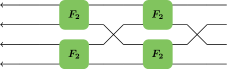
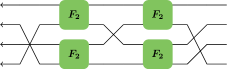
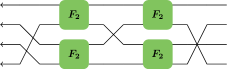
Figure 2: Dataflow of all $\operatorname{DFT}_{2}$-based linear fast algorithms computing $H_{2}$. The letters correspond to the references in Table 1

Size of $\mathcal{P}$. For a given $n$, Corollary 1 shows a direct map between $\mathcal{P}$ and $\operatorname{GL}_{n}(\mathbb{F}_{2})\times\left(\operatorname{GL}_{n-1}(\mathbb{F}_{2})\right)^{n}$. This yields the number of linear fast algorithms that compute a WHT:

$$|\mathcal{P}| =\prod_{i=0}^{n-1}(2^{n}-2^{i})\prod_{i=0}^{n-2}(2^{n-1}-2^{i})^{n}$$

$$=(2^{n+1}-2)\prod_{i=0}^{n-2}(2^{n-1}-2^{i})^{n+1}.$$

Table 2 lists the first few values of $|\mathcal{P}|$. In practice, even for relatively small $n$, this size makes any exhaustive search based approach on $\mathcal{P}$ illusive. Storing the bit-matrices of all $\operatorname{DFT}_{2}$-based linear fast algorithms computing $H_{4}$ requires $40$GB, and there are more algorithms computing $H_{6}$ than atoms in the earth.

$n$	$1$	$2$	$3$	$4$	$5$	$6$	$7$	$8$
$|\text{derived from \eqref{equ:CT}}|$	$1$	$2$	$6$	$24$	$112$	$568$	$3032$	$16768$
$|\mathcal{P}\cap\mathcal{S}_{n}^{n+1}|$	$1$	$2$	$48$	$31104$	$\approx 10^{9}$	$\approx 2\cdot 10^{15}$	$\approx 5\cdot 10^{23}$	$\approx 2\cdot 10^{34}$
$|\mathcal{P}|$	$1$	$6$	$18144$	$\approx 4\cdot 10^{12}$	$\approx 4\cdot 10^{27}$	$\approx 10^{51}$	$\approx 7\cdot 10^{84}$	$\approx 4\cdot 10^{130}$

Table 2: Number of $\operatorname{DFT}_{2}$-based linear fast algorithms $|\mathcal{P}|$, number of $\operatorname{DFT}_{2}$-based bit-index-permuted fast algorithms $|\mathcal{P}\cap\mathcal{S}_{n}^{n+1}|$ and number of algorithms that can be derived from (2) [5] for a given $n$.

1.5 Other transforms and other permutations

In this paper, we consider linearly permuted fast algorithms that compute the unscaled and naturally ordered WHT. In this section, we discuss about related algorithms, and one other set of permutations.

Walsh transform. The sequency ordered version, represented by Walsh matrix, only differs by a bit-reversal permutation of its outputs. The bit-reversal is the permutation $\pi(J_{n})$ that flips the bits of the indices:

$$J_{n}=\begin{pmatrix}&&1\\ &\iddots\\ 1\end{pmatrix}.$$

All the results obtained in this paper can be used for the Walsh matrix, after multiplying $P_{0}$ by $J_{n}$ on the left. Particularly, the number of $\operatorname{DFT}_{2}$-based linear fast Walsh transform is the same as for the WHT.

Orthogonal WHT. The WHT can be made orthogonal by scaling it by a factor of $2^{-n/2}$. Algorithms performing this transform can be obtained with our technique by using the orthogonal $\operatorname{DFT}_{2}$, i.e. the butterfly scaled by a factor of $1/\sqrt{2}$.

Bit-index permutations. Bit-index permutations are linear permutations for which the bit-matrix is itself a permutation matrix. As these are a subset of linear permutations, all the results presented here apply, and particularly, the bit-index-permuted algorithms can be enumerated using Corollary 1, but using $B\in\mathcal{S}_{n}(\mathbb{F}_{2})$ and $(Q_{1},\cdots,Q_{n})\in\left(\mathcal{S}_{n-1}(\mathbb{F}_{2})\right)^{n}$. The number of these algorithms for a given $n$ is

$$|\mathcal{P}\cap S_{n}^{n+1}|=n((n-1)!)^{n+1},$$

Table 2 gives its first few values.

2 Proof of Theorem 1

In this section, we provide a proof of Theorem  1. The main idea of this proof consists in deriving a general expression of $W(P)$, assuming only that $W(P)$ has its first row and its first column filled with $1$s (Lemma 3). Then, we match this expression with the definition of a WHT to derive necessary and necessary conditions for an algorithm to compute a WHT. Before that, in Lemma 1, we derive some consequences of the invertibility of the spreading matrix $X$, particularly on the non-zero elements of $W(P)$. In Lemma 2, we provide a necessary and sufficient condition for $W(P)$ to have a $1$-filled first row and column. We begin by defining concepts that will be used throughout this section.

Stage of an algorithm. We will refer to the stage $k$ as an array of $\operatorname{DFT}_{2}$ composed with the linear permutation associated with $P_{k}$: $(I_{2^{n-1}}\otimes\operatorname{DFT}_{2})\pi(P_{k})$. Due to the ordering of evaluation, from right to left, we call the stage $n$ is the rightmost stage of an algorithm, and the stage $k$ is on the left of the stage $k+1$. We denote with $W_{k}(P)$ the matrix corresponding to the output on the left of stage $k$, i.e.,

$$W_{k}(P)=(I_{2^{n-1}}\otimes\operatorname{DFT}_{2})\pi(P_{k})\dots(I_{2^{n-1}}\otimes\operatorname{DFT}_{2})\pi(P_{n}).$$

As a consequence, $W(P)=\pi(P_{0})W_{1}(P)$. For practical reasons, we extend this definition for $k=n+1$ by considering that $W_{n+1}(P)=I_{n}$.

Outputs depending on input $i$ on the left of stage $k$. For $0\leq i<2^{n}$, we denote with $\mathcal{D}_{k}(i)$ the set of the outputs of the $k^{th}$ stage of the algorithm that depend on the $i^{th}$ input:

$$\mathcal{D}_{k}(i)=\left\{j_{b}\mid W_{k}(P)[j,i]\neq 0\right\}\subseteq\mathbb{F}_{2}^{n}.$$

The dependency of the whole algorithm on the input $i$ is denoted with $\mathcal{D}(i)$:

$$\mathcal{D}(i)=\left\{j_{b}\mid W(P)[j,i]\neq 0\right\}.$$

Similarly, we denote with $\mathcal{D}_{k}^{+}(i)$ (resp. $\mathcal{D}_{k}^{-}(i)$) the set of the indices of the outputs for which

$$\begin{array}[]{l}\mathcal{D}_{k}^{+}(i)=\left\{j_{b}\mid W_{k}(P)[j,i]=1\right\},\text{ and }\mathcal{D}_{k}^{-}(i)=\left\{j_{b}\mid W_{k}(P)[j,i]=-1\right\}.\end{array}$$

2.1 Invertibility of the spreading matrix

In the following lemma, we justify the name “spreading matrix” that we use for $X$, by showing that its invertibility conditions the “spread” of non-zero elements through the rows of $W(P)$, and provide some other consequences we will use later.

Lemma 1.

All the outputs of the algorithm depend on the first input, i.e. $\mathcal{D}(0)=\mathbb{F}_{2}^{n}$ if and only if the spreading matrix $X$ is invertible. In this case, for every $0\leq i<2^{n}$ and $1\leq k\leq n$,

• The set of dependency at the $k^{\text{th}}$ stage on the input $i$ is

  $$\mathcal{D}_{k}(i)=(P_{k}\mathcal{D}_{k+1}(i))\cup(P_{k}\mathcal{D}_{k+1}(i)+1_{b})$$ (7)

• The non-zero elements of $W_{k}(P)$ are either $1$ or $-1$:

  $$\mathcal{D}_{k}(i)=\mathcal{D}_{k}^{+}(i)\cup\mathcal{D}_{k}^{-}(i).$$ (8)

• The $k^{\text{th}}$ stage modifies the set of dependencies such that:

  $$\mathcal{D}_{k}^{+}(i)=(P_{k}\mathcal{D}_{k+1}^{+}(i)+1_{b})\cup\{j_{b}\in P_{k}\mathcal{D}_{k+1}^{+}(i)\mid j_{b}^{T}1_{b}=0\}\cup\{j_{b}\in P_{k}\mathcal{D}_{k+1}^{-}(i)\mid j_{b}^{T}1_{b}=1\}.$$ (9)

Proof.

First, we assume that $\mathcal{D}(0)=\mathbb{F}_{2}^{n}$, and show that $X$ is invertible. For a given $j$, the two outputs $j_{b}$ and $j_{b}+1_{b}$ of a $\operatorname{DFT}_{2}$ may have a dependency on the first input only if at least one of the two signals $j_{b}$ and $j_{b}+1_{b}$ that arrive on this $\operatorname{DFT}_{2}$ depends on that input. Therefore, we have

$$\mathcal{D}_{k}(0)\subseteq P_{k}\mathcal{D}_{k+1}(0)\cup(P_{k}\mathcal{D}_{k+1}(0)+1_{b}).$$

We now prove by induction that

$$\mathcal{D}_{k}(0)\subseteq\langle 1_{b},P_{k}1_{b},P_{k:k+1}1_{b},\dots,P_{k:n-1}1_{b}\rangle.$$

We already have that $\mathcal{D}_{n+1}(0)=\{0_{b}\}$. Assuming that the result holds at rank $k+1$, we have:

$$\begin{array}[]{rcl}\mathcal{D}_{k}(0)&\subseteq&P_{k}\mathcal{D}_{k+1}(0)\cup(P_{k}\mathcal{D}_{k+1}(0)+1_{b})\\ &\subseteq&P_{k}\langle 1_{b},P_{k+1}1_{b},\dots,P_{k+1:n-1}1_{b}\rangle\cup(P_{k}\langle 1_{b},P_{k+1}1_{b},\dots,P_{k+1:n-1}1_{b}\rangle+1_{b})\\ &=&\langle P_{k}1_{b},P_{k:k+1}1_{b},\dots,P_{k:n-1}1_{b}\rangle\cup(\langle P_{k}1_{b},P_{k:k+1}1_{b},\dots,P_{k:n-1}1_{b}\rangle+1_{b})\\ &=&\langle 1_{b},P_{k}1_{b},P_{k:k+1}1_{b},\dots,P_{k:n-1}1_{b}\rangle.\end{array}$$

Which yields the result. As a consequence, we have

$$\mathcal{D}(0)=P_{0}\mathcal{D}_{1}(0)\subseteq P_{0}\langle 1_{b},P_{1}1_{b},\dots,P_{1:n-1}1_{b}\rangle=\operatorname{im}X.$$

As $\mathcal{D}(0)=\mathbb{F}_{2}^{n}$, we have $\mathbb{F}_{2}^{n}\subseteq\operatorname{im}X$, and $X$ is therefore invertible.

Conversely, we now assume that $X$ is invertible, and prove by induction that the set of outputs after stage $k$ that depend on the $i^{\text{th}}$ input is

$$\mathcal{D}_{k}(i)=P_{k:n}i_{b}+\langle 1_{b},P_{k}1_{b},P_{k:k+1}1_{b},\dots,P_{k:n-1}1_{b}\rangle.$$ (10)

We already have $\mathcal{D}_{n+1}(i)=\{i_{b}\}$. Assuming (10) for $k+1$, and considering an element

$$j_{b}\in P_{k}\mathcal{D}_{k+1}(i)=P_{k:n}i_{b}+\langle P_{k}1_{b},P_{k:k+1}1_{b},\dots,P_{k:n-1}1_{b}\rangle,$$

we have $j_{b}+P_{k:n}i_{b}\in\langle P_{k}1_{b},\dots,P_{k:n-1}1_{b}\rangle$. As $X$ is invertible, so is the matrix

$$P_{0:k-1}^{-1}X=\begin{pmatrix}P_{k:n-1}1_{b}&\cdots&P_{k}1_{b}&1_{b}&P_{k-1}^{-1}1_{b}&\cdots&P_{1:k-1}^{-1}1_{b}\end{pmatrix}.$$

Its columns are linearly independent, and particularly, $1_{b}\notin\langle P_{k}1_{b},\dots,P_{k:n-1}1_{b}\rangle$. Therefore, $j_{b}+P_{k:n}i_{b}+1_{b}\notin\langle P_{k}1_{b},\dots,P_{k:n-1}1_{b}\rangle$, thus $j_{b}+1_{b}\notin P_{k}\mathcal{D}_{k+1}(i)$. This means that if a signal $j_{b}$ that arrives on a $\operatorname{DFT}_{2}$ depends on an input $i$ ($j_{b}\in P_{k}\mathcal{D}_{k+1}(i)$), the other signal ($j_{b}+1_{b}$) doesn’t. As the output of a $\operatorname{DFT}_{2}$ is the sum (resp. the difference) of these, and that an input $i$ never appears on both terms of this operation, the dependency of both outputs on inputs is the union of the dependencies of the signals that arrive to this $\operatorname{DFT}_{2}$. This yields (7), and a direct computation shows that

$$\begin{array}[]{rcl}\mathcal{D}_{k}(i)&=&P_{k}\mathcal{D}_{k+1}(i)\cup(P_{k}\mathcal{D}_{k+1}(i)+1_{b})\\ &=&(P_{k:n}i_{b}+\langle P_{k}1_{b},\dots,P_{k:n-1}1_{b}\rangle)\cup(P_{k:n}i_{b}+\langle P_{k}1_{b},\dots,P_{k:n-1}1_{b}\rangle+1_{b})\\ &=&P_{k:n}i_{b}+\langle 1_{b},P_{k}1_{b},\dots,P_{k:n-1}1_{b}\rangle.\end{array}$$

This yields (10), and $\mathcal{D}(0)=\mathbb{F}_{2}^{n}$ as a direct consequence. To be more precise, if (8) is satisfied at rank $k+1$, a signal $j_{b}$ depending on the input $i$ that arrives on the $\operatorname{DFT}_{2}$ array of the $k^{\text{th}}$ stage is in one of these cases:

• $j_{b}\in P_{k}\mathcal{D}_{k+1}^{+}(i)$, and $j$ arrives on top of the $\operatorname{DFT}_{2}$ ($j$ is even, i.e. $j_{b}^{T}1_{b}=0$). In this case, both outputs of this $\operatorname{DFT}_{2}$ depend “positively” on $i$: $\{j_{b},j_{b}+1_{b}\}\subseteq\mathcal{D}_{k}^{+}(i)$.

• $j_{b}\in P_{k}\mathcal{D}_{k+1}^{-}(i)$, and $j$ arrives on top of the $\operatorname{DFT}_{2}$ ($j$ is even, i.e. $j_{b}^{T}1_{b}=0$). In this case, both outputs of this $\operatorname{DFT}_{2}$ depend “negatively” on $i$: $\{j_{b},j_{b}+1_{b}\}\subseteq\mathcal{D}_{k}^{-}(i)$.

• $j_{b}\in P_{k}\mathcal{D}_{k+1}^{+}(i)$, and $j$ arrives on the bottom of the $\operatorname{DFT}_{2}$ ($j$ is odd, i.e. $j_{b}^{T}1_{b}=1$). In this case, the top output depends “positively” on $i$: $j_{b}+1_{b}\in\mathcal{D}_{k}^{+}(i)$, and the bottom output “negatively”: $j_{b}\in\mathcal{D}_{k}^{-}(i)$.

• $j_{b}\in P_{k}\mathcal{D}_{k+1}^{-}(i)$, and $j$ arrives on the bottom of the $\operatorname{DFT}_{2}$ ($j$ is odd, i.e. $j_{b}^{T}1_{b}=1$). In this case, the top output depends “negatively” on $i$: $j_{b}+1_{b}\in\mathcal{D}_{k}^{-}(i)$, and the bottom output “positively”: $j_{b}\in\mathcal{D}_{k}^{+}(i)$.

This yields (9) and (8) at rank $k$. As we have as well $\mathcal{D}_{n+1}^{+}(i)\cup\mathcal{D}_{n+1}^{-}(i)=\{i_{b}\}\cup\emptyset=\mathcal{D}_{n+1}(i)$, (8) holds for all $k$. ∎

2.2 About condition (5)

As mentioned earlier, we will derive a general expression for $W(P)$, assuming that it has its first row and columns filled with $1$s. In the following theorem, we provide an equivalent condition for this assumption.

Lemma 2.

The following propositions are equivalent:

• The first row and the first column of $W(P)$ contain only $1$s:

  $$\mathcal{D}^{+}(0)=\mathbb{F}_{2}^{n},\text{ and}$$ (11)

  $$0_{b}\in\mathcal{D}^{+}(i),\text{ for }0\leq i<2^{n}.$$ (12)

• The spreading matrix satisfies (5).

• No sequential product $P_{k:\ell}$ of the central matrices has a $1$ in the bottom right corner, and the same holds for the inverse of $P_{k:\ell}$:

  $$1_{b}^{T}P_{k:\ell}1_{b}=0,\text{ for }0<k\leq\ell<n,\text{ and}$$ (13)

  $$1_{b}^{T}P_{k:\ell}^{-1}1_{b}=0,\text{ for }0<k\leq\ell<n.$$ (14)

Proof.

We start by showing the equivalence between the second and the third proposition. We consider the canonical basis $(e_{1},\dots,e_{n})$ of $\mathbb{F}_{2}^{n}$. We have, for all $0<k,k^{\prime}\leq n$,

$$e_{k}^{T}\begin{pmatrix}P_{0:n-1}^{-T}1_{b}&P_{0:n-2}^{-T}1_{b}&\dots&P_{0:1}^{-T}1_{b}&P_{0}^{-T}1_{b}\end{pmatrix}^{T}Xe_{k^{\prime}} =(P_{0:n-k}^{-T}1_{b})^{T}P_{0:n-k^{\prime}}1_{b}$$

$$=1_{b}^{T}P_{1:n-k}^{-1}P_{1:n-k^{\prime}}1_{b}$$

$$=\begin{cases}1&\text{ if }k=k^{\prime},\text{ or }\\ 1_{b}^{T}P_{n-k-1:n-k^{\prime}}1_{b}&\text{ if }k>k^{\prime},\text{ or }\\ 1_{b}^{T}P^{-1}_{n-k^{\prime}-1:n-k}1_{b}&\text{ if }k^{\prime}>k.\\ \end{cases}$$

The nullity of the two last cases is equivalent to (5) on one side, and (13) and (14) on the other side.

We now consider the first proposition. We assume first that (11) holds, and will show that it implies (13). As $\mathbb{F}_{2}^{n}=\mathcal{D}^{+}(0)\subseteq\mathcal{D}(0)$, we can use the results of Lemma 1. Using (7), (8) and (9), we have

$$\mathcal{D}_{k}^{-}(i)= \mathcal{D}_{k}(i)\setminus\mathcal{D}_{k}^{+}(i)$$

$$= \left(P_{k}\mathcal{D}_{k+1}(i)\cup(P_{k}\mathcal{D}_{k+1}(i)+1_{b})\right)\setminus$$

$$\left((P_{k}\mathcal{D}_{k+1}^{+}(i)+1_{b})\cup\{j_{b}\in P_{k}\mathcal{D}_{k+1}^{+}(i)\mid j_{b}^{T}1_{b}=0\}\cup\{j_{b}\in P_{k}\mathcal{D}_{k+1}^{-}(i)\mid j_{b}^{T}1_{b}=1\}\right)$$

$$\supseteq \left(P_{k}\mathcal{D}_{k+1}(i)+1_{b})\right)\setminus\left(P_{k}\mathcal{D}_{k+1}^{+}(i)+1_{b}\right)$$

$$= P_{k}\mathcal{D}_{k+1}^{-}(i)+1_{b}$$

Therefore, the number of outputs depending “negatively” on a given input $i$ can only increase within a stage:

$$|\mathcal{D}_{k}^{-}(i)|\geq|\mathcal{D}_{k+1}^{-}(i)|.$$

Particularly, for the first input, this means that $|\mathcal{D}^{-}(0)|=|\mathcal{D}_{1}^{-}(0)|\geq\dots\geq|\mathcal{D}_{n}^{-}(0)|$. As $\mathcal{D}^{-}(0)=\emptyset$, we have $\mathcal{D}_{k}^{+}(0)=\mathcal{D}_{k}(0)$ for all $k$. Using again (7), (8) and (9), we have, for all $k$,

$$\emptyset= \mathcal{D}_{k}^{-}(0)$$

$$= \left(P_{k}\mathcal{D}_{k+1}(0)\cup(P_{k}\mathcal{D}_{k+1}(0)+1_{b})\right)\setminus$$

$$\left((P_{k}\mathcal{D}_{k+1}^{+}(0)+1_{b})\cup\{j_{b}\in P_{k}\mathcal{D}_{k+1}^{+}(0)\mid j_{b}^{T}1_{b}=0\}\right)$$

$$= \{j_{b}\in P_{k}\mathcal{D}_{k+1}^{+}(0)\mid j_{b}^{T}1_{b}=1\},$$

Therefore, $j_{b}^{T}1_{b}=0$ for all $k$ and all $j_{b}\in P_{k}\mathcal{D}_{k+1}^{+}(0)=P_{k}\mathcal{D}_{k+1}(0)=\langle P_{k}1_{b},P_{k}P_{k+1}1_{b},\dots,P_{k:n-1}1_{b}\rangle$, which yields (13).

We now consider that (12) is satisfied. This means that (11) holds for $W(P)^{T}=W((P_{n}^{-1},\dots,P_{0}^{-1}))$, and the same computation yields (14).

Finally, we suppose that (13) and (14) hold (and therefore (5), which allows to use Lemma 1). For $i=0$, (9) becomes

$$\mathcal{D}_{k}^{+}(0)=(P_{k}\mathcal{D}_{k+1}^{+}(0)+1_{b})\cup\{j_{b}\in P_{k}\mathcal{D}_{k+1}^{+}(0)\mid j_{b}^{T}1_{b}=0\}\cup\{j_{b}\in P_{k}\mathcal{D}_{k+1}^{-}(0)\mid j_{b}^{T}1_{b}=1\}.$$

However, (13) yields that $j_{b}^{T}1_{b}=0$ in all cases. Therefore, we have

$$\mathcal{D}_{k}^{+}(0)=(P_{k}\mathcal{D}_{k+1}^{+}(0)+1_{b})\cup\{j_{b}\in P_{k}\mathcal{D}_{k+1}^{+}(0)\},$$

and a direct induction yields (11). The same argument with (14) and $W(P)^{T}$ yields (12). ∎

2.3 General expression of $W(P)$

When $X$ is invertible, we have $\mathcal{D}(i)=\mathcal{D}^{+}(i)\cup\mathcal{D}^{-}(i)$, which means that $W(P)$ is entirely determined by $\mathcal{D}^{+}$, for which we derive an expression in the following lemma.

Lemma 3.

If the spreading matrix satisfies (5), then

$$\mathcal{D}^{+}(i)=\ker\left(i_{b}^{T}P_{0:n}^{T}(XX^{T})^{-1}\right)=\left\{j_{b}\mid i_{b}^{T}P_{0:n}^{T}(XX^{T})^{-1}j_{b}=0\right\}.$$ (15)

Proof.

We assume that $X$ satisfies (5). As $X$ is invertible, the results of Lemma 1 and 2 can be used. Additionally, for $1\leq k\leq n+1$, the vectors $\{1_{b},P_{k}1_{b},P_{k:k+1}1_{b},\dots,P_{k:n-1}1_{b}\}$ are linearly independent (as columns of the invertible matrix $P_{0:k-1}^{-1}X$), and we define on the ($n-k+1$)-dimensional space spawn by these vectors the linear mapping $f_{k}$ as follows:

$$\begin{array}[]{crcl}&1_{b}&\mapsto&P^{T}_{k:n}1_{b}\\ &P_{k}1_{b}&\mapsto&P^{T}_{k+1:n}1_{b}\\ &\vdots&\vdots&\vdots\\ &P_{k:n-1}1_{b}&\mapsto&P^{T}_{n}1_{b}.\\ \end{array}$$

This mapping satisfies, for $1\leq k\leq n$, and for all $x$ in the domain of $f_{k+1}$,

$$f_{k}(P_{k}x)=f_{k+1}(x).$$ (16)

Additionally, for $k=1$, this mapping is defined over $\mathbb{F}_{2}^{n}$, and satisfies, for all $0\leq x<2^{n}$,

$$\begin{array}[]{rcl}f_{1}(x_{b})&=&\begin{pmatrix}P_{n}^{T}1_{b}&P_{n-1:n}^{T}1_{b}&\cdots&P_{1:n}^{T}1_{b}\end{pmatrix}\begin{pmatrix}P_{1:n-1}1_{b}&P_{1:n-2}1_{b}\cdots&1_{b}\end{pmatrix}^{-1}x_{b}\\ &=&P_{0:n}^{T}\begin{pmatrix}P_{0:n-1}^{-T}1_{b}&P_{0:n-2}^{-T}1_{b}&\cdots&P_{0}^{-T}1_{b}\end{pmatrix}\begin{pmatrix}P_{0:n-1}1_{b}&P_{0:n-2}1_{b}&\cdots&P_{0}1_{b}\end{pmatrix}^{-1}P_{0}x_{b}\\ &=&P_{0:n}^{T}(XX^{T})^{-1}P_{0}x_{b}.\\ \end{array}$$ (17)

We define as well the vector $s_{k}$:

$$s_{k}=1_{b}+P_{k}1_{b}+P_{k:k+1}1_{b}+\dots+P_{k:n-1}1_{b}.$$

We will now prove by induction that, for $1\leq k\leq n+1$,

$$\mathcal{D}_{k}^{+}(i)=\{j_{b}\in\mathcal{D}_{k}(i)\mid i_{b}^{T}f_{k}(j_{b}+P_{k:n}i_{b}+s_{k})=0\}.$$ (18)

We have, for $k=n+1$,

$$\begin{array}[]{rcl}\mathcal{D}_{n+1}^{+}(i)&=&\{i_{b}\}\\ &=&\{j_{b}\in\mathcal{D}_{n+1}(i)\mid i_{b}^{T}f_{n+1}(j_{b}+I_{n}i_{b}+0_{b})=0\}.\end{array}$$

If we assume that (18) is satisfied at rank $k+1$, i.e $\mathcal{D}_{k+1}^{+}(i)=\{j_{b}\in\mathcal{D}_{k+1}(i)\mid i_{b}^{T}f_{k+1}(j_{b}+P_{k+1:n}i_{b}+s_{k+1})=0\},$ we have, using (16),

$$\begin{array}[]{rcl}P_{k}\mathcal{D}_{k+1}^{+}(i)&=&\{j_{b}\in P_{k}\mathcal{D}_{k+1}(i)\mid i_{b}^{T}f_{k+1}(P_{k}^{-1}(j_{b}+P_{k:n}i_{b}+P_{k}s_{k+1}))=0\}\\ &=&\{j_{b}\in P_{k}\mathcal{D}_{k+1}(i)\mid i_{b}^{T}f_{k}(j_{b}+P_{k:n}i_{b}+P_{k}s_{k+1})=0\}.\end{array}$$

Using (8), we directly get

$$P_{k}\mathcal{D}_{k+1}^{-}(i)=\{j_{b}\in P_{k}\mathcal{D}_{k+1}(i)\mid i_{b}^{T}f_{k}(j_{b}+P_{k:n}i_{b}+P_{k}s_{k+1})=1\}.$$

We can now compute $\mathcal{D}_{k}^{+}$ using (9):

$$\begin{array}[]{rcl}\mathcal{D}_{k}^{+}(i)&=&(P_{k}\mathcal{D}_{k+1}^{+}(i)+1_{b})\cup\{j_{b}\in P_{k}\mathcal{D}_{k+1}^{+}(i)\mid j_{b}^{T}1_{b}=0\}\cup\{j_{b}\in P_{k}\mathcal{D}_{k+1}^{-}(i)\mid j_{b}^{T}1_{b}=1\}\\ &=&(P_{k}\mathcal{D}_{k+1}^{+}(i)+1_{b})\cup\{j_{b}\in P_{k}\mathcal{D}_{k+1}(i)\mid i_{b}^{T}f_{k}(j_{b}+P_{k:n}i_{b}+P_{k}s_{k+1})+j_{b}^{T}1_{b}=0\}.\\ \end{array}$$

The term $j_{b}^{T}1_{b}$ that appears for $j_{b}\in P_{k}\mathcal{D}_{k+1}(i)=P_{k:n}i_{b}+\langle P_{k}1_{b},P_{k:k+1}1_{b},\dots,P_{k:n-1}1_{b}\rangle$ satisfies, using (13), $j_{b}^{T}1_{b}=i_{b}^{T}P_{k:n}^{T}1_{b}=i_{b}^{T}f_{k}(1_{b})$. Therefore:

$$\begin{array}[]{rcl}\mathcal{D}_{k}^{+}(i)&=&(P_{k}\mathcal{D}_{k+1}^{+}(i)+1_{b})\cup\{j_{b}\in P_{k}\mathcal{D}_{k+1}(i)\mid i_{b}^{T}f_{k}(j_{b}+P_{k:n}i_{b}+P_{k}s_{k+1})+i_{b}^{T}f_{k}(1_{b})=0\}\\ &=&(P_{k}\mathcal{D}_{k+1}^{+}(i)+1_{b})\cup\{j_{b}\in P_{k}\mathcal{D}_{k+1}(i)\mid i_{b}^{T}f_{k}(j_{b}+P_{k:n}i_{b}+s_{k})=0\}\\ &=&\{j_{b}\in P_{k}\mathcal{D}_{k+1}(i)+1_{b}\mid i_{b}^{T}f_{k}(j_{b}+P_{k:n}i_{b}+s_{k})=0\}\cup\\ &&\{j_{b}\in P_{k}\mathcal{D}_{k+1}(i)\mid i_{b}^{T}f_{k}(j_{b}+P_{k:n}i_{b}+s_{k})=0\}\\ &=&\{j_{b}\in\mathcal{D}_{k}(i)\mid i_{b}^{T}f_{k}(j_{b}+P_{k:n}i_{b}+s_{k})=0\},\end{array}$$

which yields the result.

We can now provide a first expression for $\mathcal{D}^{+}$, using (16):

$$\begin{array}[]{rcl}\mathcal{D}^{+}(i)&=&P_{0}\mathcal{D}^{+}_{1}(i)\\ &=&P_{0}\{j_{b}\mid i_{b}^{T}f_{1}(j_{b}+P_{1:n}i_{b}+s_{1})=0\}\\ &=&P_{0}\{j_{b}\mid i_{b}^{T}P_{0:n}^{T}(XX^{T})^{-1}(P_{0}j_{b}+P_{0:n}i_{b}+P_{0}s_{1})=0\}\\ &=&\{j_{b}\mid i_{b}^{T}P_{0:n}^{T}(XX^{T})^{-1}(j_{b}+P_{0:n}i_{b}+P_{0}s_{1})=0\}.\\ \end{array}$$

The last step consists in showing that the mapping $g:i_{b}\mapsto i_{b}^{T}P_{0:n}^{T}(XX^{T})^{-1}(P_{0:n}i_{b}+P_{0}s_{1})$ is null. We consider the canonical basis $(e_{1},\dots,e_{n})$ of $\mathbb{F}_{2}^{n}$, and a vector $x=\sum_{i}\lambda_{i}P_{0:n}^{-1}Xe_{i}$ of this space. A direct computation yields:

$$g(x) =x^{T}P_{0:n}^{T}(XX^{T})^{-1}(P_{0:n}x+P_{0}s_{1})$$

$$=(X^{-1}P_{0:n}x)^{T}X^{-1}(P_{0:n}x+P_{0}s_{1})$$

$$=\left(X^{-1}P_{0:n}\sum_{i}\lambda_{i}P_{0:n}^{-1}Xe_{i}\right)^{T}X^{-1}\left(P_{0:n}\sum_{j}\lambda_{j}P_{0:n}^{-1}Xe_{j}+\sum_{k}Xe_{k}\right)$$

$$=\sum_{i}\lambda_{i}e_{i}^{T}\sum_{j}(\lambda_{j}+1)e_{j}$$

$$=\sum_{i,j}\lambda_{i}(\lambda_{j}+1)e_{i}^{T}e_{j}$$

$$=\sum_{i=j}\lambda_{i}(\lambda_{j}+1)e_{i}^{T}e_{j}+\sum_{i\neq j}\lambda_{i}(\lambda_{j}+1)e_{i}^{T}e_{j}$$

$$=0.$$

∎

2.4 Proof of theorem 1

The proof of theorem 1 is now straightforward.

If $P\in\mathcal{P}$, then $W(P)$ has its first column and row filled up with $1$s. Lemma 2 ensures (5), and we can use Lemma 3. Identifying (15) with the definition (1) of $H_{n}$ yields that $P_{0:n}^{T}=XX^{T}$, i.e. that (4) is satisfied.

Conversely, if (4) and (5) are satisfied, $W(P)=H_{n}$ is a direct consequence of Lemma 3.

3 Proof of Corollary 1

We first assume that $(P_{0},\dots,P_{n})\in\mathcal{P}$, and construct a set of matrices satisfying (6). We define $B=X^{-1}$, and, by induction, the matrices

$$\tilde{Q}_{i}=\begin{cases}B^{-1}\cdot P_{0},&\text{ for }i=1,\\ C_{n}^{-1}\cdot\tilde{Q}_{i-1}\cdot P_{i-1},&\text{ for }1<i\leq n.\\ \end{cases}$$

By construction, these matrices satisfy, for $0<i\leq n$, $\tilde{Q}_{i}=C_{n}^{1-i}X^{-1}P_{0:i-1}$. Using (4), we get:

$$P_{i}=\begin{cases}B\cdot\tilde{Q}_{1},&\text{ for }i=0,\\ \tilde{Q}_{i}^{-1}\cdot C_{n}\cdot\tilde{Q}_{i+1},&\text{ for }0<i<n,\\ \tilde{Q}_{n}^{-1}\cdot C_{n}\cdot\tilde{B}^{T},&\text{ for }i=n.\\ \end{cases}$$

The last step consists in showing that, for $0<i\leq n$, there exists a matrix $Q_{i}\in\operatorname{GL}_{n-1}(\mathbb{F}_{2})$ such that $\tilde{Q}_{i}=\begin{pmatrix}Q_{i}&\\ &1\end{pmatrix}$, or equivalently, that $\tilde{Q}_{i}1_{b}=\tilde{Q}_{i}^{T}1_{b}=1_{b}$:

$$\tilde{Q}_{i}1_{b} =C_{n}^{1-i}X^{-1}P_{0:i-1}1_{b}$$

$$=C_{n}^{1-i}\begin{pmatrix}P_{0:n-1}1_{b}&\dots&P_{0:1}1_{b}&P_{0}1_{b}\end{pmatrix}^{-1}P_{0:i-1}1_{b}$$

$$=1_{b}.$$

A similar computation, using (5), shows that $\tilde{Q}_{i}^{T}1_{b}=1_{b}$.

Conversely, if a set of matrices satisfy (6), a direct computation (with [4]) shows that (4) and (5) are satisfied. Thus. $P\in\mathcal{P}$.

4 Conclusion

We described a method to characterize and enumerate fast linear WHT algorithms. As methods are known to implement optimally linear permutations on hardware [9], a natural future work would consist in finding the best WHT algorithm that can be implemented for a given $n$. Additionally, it would be interesting to see if similar algorithms exist for other transforms, like the $\operatorname{DFT}$.

References

• [1] K. G. Beauchamp. Applications of Walsh and related functions with an introduction to sequency theory. Academic Press, 1985.
• [2] James W. Cooley and John W. Tukey. An algorithm for the machine calculation of complex Fourier series. Mathematics of Computation, 19(90):297–301, 1965.
• [3] Jacques Hadamard. Résolution d’une question relative aux déterminants. Bulletin des sciences mathématiques, 17:240–246, 1893.
• [4] J. R. Johnson, R. W. Johnson, D. Rodriguez, and R. Tolimieri. A methodology for designing, modifying, and implementing Fourier transform algorithms on various architectures. Circuits, Systems and Signal Processing, 9(4):449–500, Dec 1990.
• [5] Jeremy Johnson and Markus Püschel. In search of the optimal Walsh-Hadamard transform. In International Conference on Acoustics, Speech, and Signal Processing (ICASSP), volume 6, pages 3347–3350, 2000.
• [6] Florence Jessie MacWilliams and Neil James Alexander Sloane. The theory of error-correcting codes. Elsevier, 1977.
• [7] Marshall C. Pease. An adaptation of the fast Fourier transform for parallel processing. Journal of the ACM, 15(2):252–264, April 1968.
• [8] Markus Püschel, Peter A. Milder, and James C. Hoe. Permuting streaming data using RAMs. Journal of the ACM, 56(2):10:1–10:34, 2009.
• [9] François Serre, Thomas Holenstein, and Markus Püschel. Optimal circuits for streamed linear permutations using RAM. In International Symposium on Field-Programmable Gate Arrays (FPGA), pages 215–223. ACM, 2016.