Determination of Dark Matter Halo Mass from Dynamics of Satellite Galaxies

Abstract

We show that the mass of a dark matter halo can be inferred from the dynamical status of its satellite galaxies. Using 9 dark-matter simulations of halos like the Milky Way (MW), we find that the present-day substructures in each halo follow a characteristic distribution in the phase space of orbital binding energy and angular momentum, and that this distribution is similar from halo to halo but has an intrinsic dependence on the halo formation history. We construct this distribution directly from the simulations for a specific halo and extend the result to halos of similar formation history but different masses by scaling. The mass of an observed halo can then be estimated by maximizing the likelihood in comparing the measured kinematic parameters of its satellite galaxies with these distributions. We test the validity and accuracy of this method with mock samples taken from the simulations. Using the positions, radial velocities, and proper motions of 9 tracers and assuming observational uncertainties comparable to those of MW satellite galaxies, we find that the halo mass can be recovered to within $\sim 40$%. The accuracy can be improved to within $\sim$25% if 30 tracers are used. However, the dependence of the phase-space distribution on the halo formation history sets a minimum uncertainty of $\sim 20$% that cannot be reduced by using more tracers. We believe that this minimum uncertainty also applies to any mass determination for a halo when the phase space information of other kinematic tracers is used.

1 Introduction

We present a method to estimate the mass of a dark matter halo from the dynamical status of its satellite galaxies. In the framework of hierarchical structure formation based on the concordance cold dark matter ($\Lambda\mathrm{CDM}$) cosmology, the mass of a dark matter halo is closely related to its many other properties such as structure, dynamics, and formation history. In the case of the Milky Way (MW), a number of theoretical predictions or interpretations of observations, for example, the baryon fraction (e.g. Zaritsky & Courtois, 2017) and the problem of missing massive satellites (e.g. Boylan-Kolchin et al., 2011; Wang et al., 2012; Cautun et al., 2014), depend on the MW halo mass. Various methods have been proposed to measure this important quantity (see Courteau et al. 2014; Bland-Hawthorn & Gerhard 2016 for reviews and Wang et al. 2015 for a comparison of recent measurements). Though these measurements are roughly consistent, they result in a factor of $\sim 3$ difference in the estimated MW halo mass. The scatter might be even larger if systematic uncertainties are included (Han et al., 2016b; Wang et al., 2016). Clearly, there is a need for more accurate methods to determine the MW halo mass.

The MW halo mass can be constrained by the abundances of certain constituents, such as the baryon fraction (Zaritsky & Courtois, 2017), the total stellar mass (Guo et al., 2011), and the number of satellite galaxies above a specific threshold (e.g. Starkenburg et al., 2013; Rodriguez-Puebla et al., 2013; Cautun et al., 2014). Timing argument is widely used to give another mass estimator by modeling the expansion of the Local Group galaxies (Kahn & Woltjer, 1959; Li & White, 2008; Peñarrubia et al., 2016; Banik & Zhao, 2016). Perhaps the most powerful and direct method to estimate the MW halo mass is to use dynamical tracers. In this regard, the mass distribution within $\sim 100$ kpc is reasonably well constrained by the kinematics of stars (e.g. Xue et al., 2008; Huang et al., 2016) or a stellar stream (e.g. Gibbons et al., 2014). However, due to the limited spatial distribution of these tracers, extrapolation is needed to obtain the total halo mass, which often depends on the assumed parametric form for the overall density profile.

The outer region of the MW can be investigated more directly by using its satellite galaxies, which lie far beyond the other tracers. However, this approach was limited for a long time by the small sample size, large uncertainties in distance estimates, and lack of proper-motion measurement. Fortunately, both the sample size and precision of distance measurement have increased greatly over the past decade (see McConnachie 2012 for a recent compilation of observations). In addition, with the unprecedented precision of the HST and the new generation of ground-based telescopes, proper motions of bright satellites have been measured (e.g. Piatek et al. 2002, 2003, 2005, also see Table 1 of Pawlowski & Kroupa 2013 for a summary of currently available measurements). Consequently, such satellites are fully characterized in the 6D phase space of position and velocity and their orbits can be computed assuming a potential. Currently, proper motions are available for 12 of the 13 satellite galaxies (the exception being Canes Venatici I) that are more luminous than $10^{5}L_{\odot}$ and within 300 kpc from the MW center.

However, unlike stellar tracers, the limited number of satellite galaxies does not allow direct calculation of the velocity dispersion profile or rotation curve. Instead, analytical models of the dynamical status or comparisons with numerical simulations are required. Previous studies using satellite galaxies considered the orbital energy of Leo I (Boylan-Kolchin et al., 2013), velocity moments (Watkins et al., 2010), orbital ellipticity distribution (Barber et al., 2014), and probability distribution of orbital parameters (Eadie et al., 2015, 2016). These approaches encounter several difficulties. When the density and velocity anisotropy profiles of the tracer population are assumed, the inferred mass distribution depends sensitively on the assumptions (e.g. Watkins et al., 2010; Eadie et al., 2016), which requires further systematic study. In addition, analytical methods assume that all satellites are bound in a steady state with random orbital phases, which may not hold for all halos. The influence of deviations from a steady state and halo-to-halo scatter has yet to be taken into full consideration. Another difficulty is how to treat observational errors properly, as the measurement uncertainty differs substantially from satellite to satellite. In this paper we develop a new method that either avoids or addresses the above issues in using satellite galaxies to estimate the MW halo mass.

We base our method on dark-matter simulations of MW-like halos and associate satellite galaxies with subhalos of a simulated halo. We construct the distribution of subhalos in the phase space of orbital binding energy and angular momentum directly from the simulations without assuming a steady state or any particular form of velocity anisotropy. We also take into account observational uncertainties of satellite galaxies. We estimate the halo mass by maximizing the likelihood in comparing the observed orbital parameters of satellite galaxies with the phase-space distribution derived from simulations. We test the validity of this method and investigate its systematics using mock samples taken from simulations. We also study the dependence of this halo mass estimator on observational uncertainties, the number of satellites used, and halo-to-halo scatter. While our method is motivated by improving the estimate of the MW halo mass, it can be extended to other MW-like halos as well.

The plan of this paper is as follows. We outline our method in Section 2 and show how to construct the phase-space distribution of subhalos from simulations in Section 3. We discuss systematic tests by mock samples in Section 4 and give conclusions in Section 5.

2 Method

Our basic assumption is that for a present-day halo of mass $M_{\mathrm{h}}$, its substructures have a characteristic distribution $p(E,L|M_{\mathrm{h}})$ in the phase space of orbital binding energy $E$ and angular momentum $L$ (see below for definition). Then the unknown mass of a halo can be inferred by comparing the observed orbital parameters of its substructure tracers with the phase-space distributions derived from simulations for different $M_{\mathrm{h}}$. In practice, dwarf satellite galaxies are the outmost tracers for the MW. To develop the halo mass estimator, we consider such satellites as a subset of the surviving subhalos for a halo in terms of kinematics. Hereafter, the simulated halo that provides the calculated phase-space distribution is referred to as the template halo. The halo whose mass is to be determined is referred to as the test halo.

We characterize the orbit in the potential of a halo by the corresponding binding energy $E$ and angular momentum $L$ per unit mass. Specifically,

$$\begin{split}&E=-\Phi(r)-\frac{1}{2}(v_{\mathrm{r}}^{2}+v_{\mathrm{t}}^{2}),\\ &L=rv_{\mathrm{t}},\end{split}$$ (1)

where $r$, $v_{\mathrm{r}}$, and $v_{\mathrm{t}}$ are the distance, the radial and tangential velocity relative to the center of the host halo, respectively, and

$$\Phi(r)=-\int_{r}^{r_{0}}\frac{GM_{\Delta}(r^{\prime})}{r^{\prime 2}}\mathrm{d}r^{\prime}$$ (2)

is the gravitational potential. In the above equation, $r_{0}$ corresponds to the zero potential point, $G$ is the gravitational constant, and

$$M_{\Delta}(r)=\int_{0}^{r}4\pi[\rho(r^{\prime})-\bar{\rho}]r^{\prime 2}\mathrm{d}r^{\prime}$$ (3)

represents the mass exceeding the mean cosmic background, where $\rho(r)$ is the dark matter density profile of the host halo and $\bar{\rho}$ is the mean cosmic density. We adopt $r_{0}=1h^{-1}\,\mathrm{Mpc}$ and have checked that using $r_{0}=3h^{-1}\,\mathrm{Mpc}$ instead makes little difference in the results.

There are two reasons why we do not use the observable parameters $r$, $v_{\mathrm{r}}$, and $v_{\mathrm{t}}$ directly although this alternative seems to provide more information. First, the $E$ and $L$ of a subhalo are approximately conserved after its infall into the host halo. They are less mixed in phase space over time and also less sensitive to individual merger events that produce halo-to-halo scatter. Second, due to the finite number of subhalos in the simulations, the constructed phase space of $r$, $v_{\mathrm{r}}$, and $v_{\mathrm{t}}$ is more sparse, and therefore, more discontinuous. This problem is mitigated by using the phase space of the corresponding $E$ and $L$ instead. Hereafter, “phase space” means $E$-$L$ space.

For a template halo of mass $M_{\mathrm{h}}$, we construct the phase-space distribution $p(E,L|M_{\mathrm{h}})$ directly from the simulations. Specifically,

$$p(E,L|M_{\mathrm{h}})=\frac{1}{n_{\mathrm{sub}}}\sum_{i=1}^{n_{\mathrm{sub}}}\tilde{p}(E,L|\mathrm{sub}_{i}),$$ (4)

where $n_{\mathrm{sub}}$ is the number of selected subhalos, and $\tilde{p}(E,L|\mathrm{sub}_{i})$ represents the probability density for the $i$-th subhalo to be “observed” at $(E,L)$. As described in detail in Section 3, $\tilde{p}(E,L|\mathrm{sub}_{i})$ serves as the kernel function in the kernel density estimation to transform the discrete distribution of subhalos in phase space into a continuous one.

The utility of template halos is greatly extended by the scaling technique. For the mass range of our interest for the Milky Way halo, dark-matter halos are built up approximately in a self-similar manner, thus we can scale a halo to a different mass while keeping the formation history and relaxation status unchanged. Specifically, the distribution $p(E,L|M_{\mathrm{h}}^{\prime})$ for a halo of mass $M_{\mathrm{h}}^{\prime}$ can be obtained from $p(E,L|M_{\mathrm{h}})$ by using

$$\begin{split}r^{\prime}=(M_{\mathrm{h}}^{\prime}/M_{\mathrm{h}})^{1/3}r,\\ v_{\mathrm{r(t)}}^{\prime}=(M_{\mathrm{h}}^{\prime}/M_{\mathrm{h}})^{1/3}v_{\mathrm{r(t)}},\\ \Phi^{\prime}=(M_{\mathrm{h}}^{\prime}/M_{\mathrm{h}})^{2/3}\Phi,\end{split}$$ (5)

for each of the subhalos in the halo of mass $M_{\mathrm{h}}$. The subhalo mass is scaled as $m^{\prime}=(M_{\mathrm{h}}^{\prime}/M_{\mathrm{h}})m$. In this way, we can construct a family of distributions $p(E,L|M_{\mathrm{h}}^{\prime})$ for a range of halo mass $M_{\mathrm{h}}^{\prime}$ from a single template halo.

To infer the unknown mass of a test halo hosting a set of satellites with observed $(r,v_{r},v_{t})$, we calculate $(E,L)$ for each satellite using the potential of a scaled template halo of mass $M_{\mathrm{h}}^{\prime}$ and further compute the likelihood

$$\mathcal{L}(\mathrm{obs}|M_{h}^{\prime})=\prod^{N_{\mathrm{sat}}}_{k=1}p(E_{k},L_{k}|M_{h}^{\prime}),$$ (6)

where $N_{\mathrm{sat}}$ is the number of observed satellites, and $(E_{k},L_{k})$ correspond to the $k$-th satellite. The likelihood $\mathcal{L}(\mathrm{obs}|M_{\mathrm{h}}^{\prime})$ can be calculated for a range of template halos scaled to different $M_{\mathrm{h}}^{\prime}$. Assuming that the test halo has the same formation history and relaxation status as the template halos, we can infer the unknown mass of the test halo by maximizing $\mathcal{L}(\mathrm{obs}|M_{\mathrm{h}}^{\prime})$, which gives the Maximum Likelihood Estimator (MLE) for the mass

$$M_{\mathrm{esti}}=\arg\max_{M_{\mathrm{h}}^{\prime}}\mathcal{L}(\mathrm{obs}|M_{\mathrm{h}}^{\prime}).$$ (7)

The above method is illustrated by Figure 1, which shows how $\mathcal{L}(\mathrm{obs}|M_{\mathrm{h}}^{\prime})$ changes with $M_{\mathrm{h}}^{\prime}$. Template halo A1 in our simulations, which has a true mass of $M_{h}\approx 1.6\times 10^{12}M_{\odot}$, is also used as a test halo and its most massive 9 subhalos are chosen as satellites, for which mock observations of $(r,v_{r},v_{t})$ are made with the fiducial measurement precision (see Section 3.3 and Section 3.4). The colored contours in Figure 1 represent the phase-space distribution constructed from template halo A1 by scaling it to $M_{\mathrm{h}}^{\prime}=0.5\times 10^{12}$, $1.5\times 10^{12}$, and $2.5\times 10^{12}M_{\odot}$, respectively. The symbols stand for the mock data on $(E,L)$ for the satellites. Note that the “observed” $(r,v_{r},v_{t})$ for each satellite do not change during scaling. Therefore, the mock data on $L$ remain the same but those on $E$ change with the potential of the scaled template halo. The observation points become more bound as $M_{\mathrm{h}}^{\prime}$ increases. It can be seen from Figure 1 that among the three $M_{\mathrm{h}}^{\prime}$ values, the likelihood of the observations is the largest for the middle one, which is also closest to the true value $M_{\mathrm{h}}$.

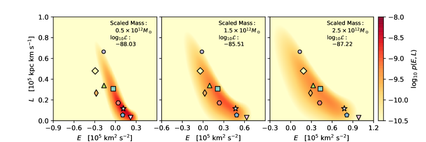
Figure 1: Comparison of mock observations with the phase-space distributions constructed from simulations of template halo A1 scaled to different halo masses. Template halo A1 is also used as a test halo and its most massive 9 subhalos are chosen as satellites for mock observations. Symbols with black border and colored contours represent mock data and constructed phase-space distributions, respectively. The scaled halo mass and the corresponding likelihood of mock observations are shown in each panel. It can be seen that among the three cases, the likelihood is the largest for the middle one, whose halo mass is also closest to the true value of $\approx 1.6\times 10^{12}M_{\odot}$.

Because the binding energy $E$ of a satellite depends on the template halo mass $M_{\mathrm{h}}^{\prime}$, the likelihood $\mathcal{L}(\mathrm{obs}|M_{\mathrm{h}}^{\prime})$ cannot be converted in a straightforward manner into the probability distribution of the true halo mass even when the prior distribution of $M_{\mathrm{h}}^{\prime}$ is known. Nevertheless, we will show that the MLE $M_{\mathrm{esti}}$ is indeed a good, though biased, indicator for the true halo mass. Using Monte Carlo realization of mock samples, we find that the bias is approximately constant and define an average bias $\eta=\left\langle M_{\mathrm{esti}}/M_{\mathrm{true}}\right\rangle$ over the mock samples. Consequently, we obtain the bias-corrected estimator for the halo mass

$$\hat{M}_{\mathrm{esti}}=M_{\mathrm{esti}}/\eta.$$ (8)

The above discussion assumes that the test and template halos have the same formation history and relaxation status. However, such information about the test halo is not readily available in practice. The lack of such information then introduces an intrinsic uncertainty into our method. We assess this uncertainty using 9 simulated halos with a wide range of formation history in Section 4.

3 Construction of Subhalo Phase-Space Distribution

Central to our method is the phase-space distribution $p(E,L|M_{\mathrm{h}})$ of subhalos for a template halo of mass $M_{\mathrm{h}}$. This distribution is constructed directly from our simulations taking into account realistic observational uncertainties. The detailed procedure is described in this section.

3.1 Simulations

In order to have enough substructures within a halo and resolve them with reasonable details, we use the cosmological N-body simulation of Jing & Suto (2002) to select nine template halos for high-resolution resimulations. Each of these halos is required to be relatively isolated at redshift $z=0$ so that its distance to any more massive halo must exceed three times the sum of the virial radii of both halos. In addition, each template halo is required to have a mass of approximately $1.5\times 10^{12}M_{\odot}$ similar to that of the MW. The simulation was performed in a box of $100h^{-1}\,\mathrm{Mpc}$ on each side with a parallel particle-particle-particle-mesh $\rm{P^{3}M}$ code using $512^{3}$ particles. A $\Lambda\mathrm{CDM}$ cosmology was adopted with the density parameter $\Omega_{m}=0.3$, the cosmological constant $\Omega_{\Lambda}=0.7$, the Hubble constant $h=0.67$ in units of $100\ \mathrm{km\,s}^{-1}\mathrm{Mpc}^{-1}$, and the slope $n_{s}=1$ and amplitude $\sigma_{8}=0.9$ of the primordial power spectrum. While these parameters are not up to date, they are close to the most recent results from the Planck mission. The differences in the cosmological parameters have little effect on the conclusions of this study because our main concern is to develop a method of estimating halo masses and test its validity. For each template halo, we use the multiple-mass method to generate the initial conditions for zooming (Jing & Suto, 2000) and carry out zoom-in resimulations using the public code Gadget2 (Springel, 2005). In the high-resolution region enclosing a template halo, these simulations have a particle mass of $\sim 10^{5}M_{\odot}$ (Table 1) and a softening length of 0.15 $h^{-1}\,\mathrm{kpc}$.

We find halos using the standard Friends-of-Friends (FoF) algorithm with a linking length $b$ equal to 0.2 times the mean separation of high-resolution particles. For ease of comparison with results in the literature, we define $M_{\mathrm{h}}$ and $R_{\mathrm{h}}$ as the mass and radius, respectively, of a spherical region with a mean density equal to 200 times the critical density of the universe. The 9 template halos have $M_{\mathrm{h}}\sim(1.3$–$1.6)\times 10^{12}M_{\odot}$ (Table 1) within $R_{\mathrm{h}}\sim 230$ kpc at $z=0$. As shown in Figure 2 and Table 1, these halos have very different histories of mass growth, and therefore, cover a wide range of possible assembly history for an MW-like halo. Lacking the formation history of a test halo, we must resort to exploring a wide range of template halos to investigate the uncertainty from halo-to-halo scatter in our method of halo mass determination.

We use the Hierarchical Bound-Tracing (HBT) algorithm of Han et al. (2012) to identify subhalos and build merger trees through time in the simulations. HBT traces merger hierarchy of halos and subhalos with a physically-motivated unbinding algorithm, and thus has robust performance even in the dense inner region of a host halo, which fits our needs very well. The mass $m$ of a subhalo is defined to be its self-bound mass. A subhalo can be identified if it contains at least 10 bound particles ($\sim 10^{6}M_{\odot}$). The positions and velocities of subhalos are essential input to construction of their phase-space distribution. These quantities are defined in HBT by the center of mass and bulk velocity of the most bound 25% of the particles in each subhalo (see Han et al. 2012 for details). The center of the largest subhalo is taken as the center of its host halo.

We have checked the completeness of subhalo samples in the high-resolution region of the zoom-in simulations. As expected (Han et al., 2016a), within $2R_{h}$, the number density profile of subhalos (including disrupted ones) in any given infall-mass bin coincides very well with the dark-matter density profile of the host halo. Therefore, the subhalo sample within $2R_{h}$ is complete and not affected by the low-resolution particles.

Table 1: Properties of Template Halos

Halo	$m_{p}$	$M_{h}$	$t_{0.5}$	$t_{0.8}$
	$(10^{5}M_{\odot})$	$(10^{12}M_{\odot})$	$(\mathrm{Gyr})$	$(\mathrm{Gyr})$
A1	0.99	1.58	3.14	1.79
A2	1.11	1.46	6.95	3.58
A3	0.96	1.61	9.21	5.06
A4	0.93	1.60	10.20	3.96
A5	0.96	1.60	10.55	6.65
A6	1.37	1.54	6.93	6.68
A7	1.02	1.55	1.42	1.09
A8	1.05	1.64	9.54	9.13
A9	0.92	1.38	2.71	2.46

Note. — The columns are the particle mass $m_{p}$ in the high-resolution region, the present ($z=0$) mass $M_{h}$ of the template halo, the lookback times $t_{0.5}$ and $t_{0.8}$ when the halo first reached 50% and 80% of its present mass, respectively.

Figure 2: Growth history of template halos. The solid curves color-coded A1–A9 show the fraction of the present halo mass as a function of the lookback time $t$ for the corresponding halos. For reference, the dashed curve shows the median growth history for halos of $1.5\times 10^{12}M_{\odot}$ in the model of Zhao et al. (2009).

3.2 Subhalo sample selection

As satellite galaxies are intended as the subhalo tracers, we adopt the following criteria to mimic these tracers in selecting the subhalos to construct the phase-space distribution for a template halo.

• Maximum binding mass in history: $m_{\max}>2\times 10^{-5}M_{h}$ ($\gtrsim 300$ particles)

  Subhalos containing only $\sim 10$ particles are vulnerable to numerical instability. As shown by Han et al. (2016a), at infall a subhalo should be at least $\sim 30$ times more massive than the smallest resolved subhalo to alleviate artificial disruptions. On the other hand, we would like to keep enough subhalos to have good statistics. The above relatively low mass threshold is adopted as a reasonable compromise. We note that subhalos hosting the bright MW dwarf galaxies were probably $\sim 100$ times larger than this limit at their infall. We will show that our method is not very sensitive to this mass selection.

• Mass at $z=0$: $m_{0}\gtrsim 10^{6}M_{\odot}$ ($>10$ particles)

  This is a safe lower bound, as MW dwarf galaxies have high mass-to-light ratios (e.g. Wolf et al., 2010), with the mass enclosed within 300 pc being $\sim 10^{7}M_{\odot}$ for most of these satellites (Strigari et al., 2008) and that within the half-light radius being $\gtrsim 5\times 10^{6}M_{\odot}$ for the classical dwarf galaxies (McConnachie, 2012). We have checked that doubling the lower bounds on $m_{\max}$ and $m_{0}$ changes the results by only $\lesssim 5\%$.

• Distance to host halo center: $40\ \mathrm{kpc}<r<300\ \mathrm{kpc}$

  This range covers the 9 MW satellites with adequate kinematic data and excludes satellites experiencing strong tidal disruption due to extreme proximity to the Galactic Center (GC) (see Section 3.3). As the absolute position of a subhalo changes with the scaled halo mass, this criterion makes the selected subhalo sample dependent on the scaling of a template halo. Consequently, to ensure completeness of the sample, a scaled template halo must satisfy $2R_{h}>300\ \mathrm{kpc}$, which limits the scaled halo mass to $M_{h}>0.35\times 10^{12}M_{\odot}$. This lower bound is below the expected MW halo mass and does not pose any limitation in practice.

The dots in Figure 3 show the discrete phase-space distribution of subhalos selected according to the above criteria for each of the 9 template halos in our simulations. These distributions share broad similarity, but significant differences exist. The similarity points to a basic dependence on the halo mass while the differences reflect the halo-to-halo scatter that must be taken into account in our method of halo mass determination. There appears to be a crude relation between the dynamical status of subhalos and the formation history of the host halo: the phase space is more extended and there are more unbound subhalos in late-formed halos such as A7 and A9 (Table 1).

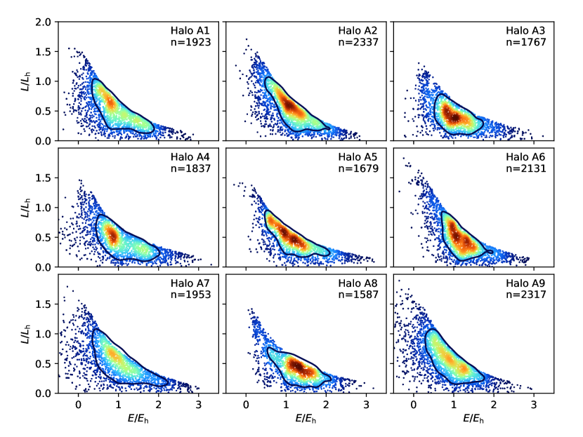
Figure 3: Discrete phase-space distribution of subhalos for each of the template halos A1–A9. The units of $E$ and $L$ are $E_{h}=GM_{h}/R_{h}$ and $L_{h}=\sqrt{GM_{h}R_{h}}$ , respectively. The number $n$ of subhalos in the selected sample is indicated for each halo. Each dot represents a subhalo and is colored according to the local number density in the phase space with red indicating higher density and the same color normalization for all halos. The curve is the equidensity contour enclosing half of the subhalos. The distributions show broad similarity but also clear differences.

3.3 Observational Guidance

A practical application of the method presented in this paper is to estimate the mass of the MW halo. We use the current observations of the MW and its satellite galaxies as a guide in developing the method.

There are 13 satellite galaxies more luminous than $10^{5}L_{\odot}$ within 300 kpc of the GC. Proper motions are available for 12 of these with the exception being Canes Venatici I (Pawlowski & Kroupa, 2013). We exclude Sextans due to the very large uncertainty in its proper motion. Canis Major and Sagittarius are also excluded because they are so close to the GC that they are experiencing strong tidal disruption. Consequently, 9 satellite galaxies of the MW can be used as subhalo tracers at present. Among these, the Large Magellanic Cloud (LMC) at $50\pm 2\ \mathrm{kpc}$ is the closest to the GC while Leo I at $258\pm 15\ \mathrm{kpc}$ is the farthermost (McConnachie, 2012).

For developing our method to estimate the mass of a test halo based on comparison of the kinematic properties of its subhalos with the phase-space distributions of template halos, the most pertinent guidance provided by current observations of MW satellite galaxies is the number of these tracers with sufficiently accurate kinematic data and the typical uncertainties in such data. We adopt the following fiducial values characteristic of current observations.

1. The number of tracers with adequate kinematic data is

   $$N=9.$$ (9)

2. The relative uncertainty in the distance to the Sun in the Heliocentric Standard of Rest (HSR) is

   $$(\sigma_{r}/r)_{\rm HSR}=0.06.$$ (10)

3. The measurement error of the radial velocity with respect to HSR is

   $$(\sigma_{v_{\mathrm{los}}})_{\rm HSR}=1\ \mathrm{km\,s}^{-1}.$$ (11)

4. The precision for the proper motion components with respect to HSR is

   $$(\sigma_{\mu_{\alpha}})_{\rm HSR}=(\sigma_{\mu_{\delta}})_{\rm HSR}=0.08\ \mathrm{mas\,yr}^{-1}.$$ (12)

The uncertainties $(\sigma_{r}/r,\sigma_{v_{\mathrm{los}}},\sigma_{\mu_{\alpha}},\sigma_{\mu_{\delta}})_{\rm HSR}$ adopted above are approximately the root-mean-square values of current precisions for luminous MW satellite galaxies (Pawlowski & Kroupa, 2013). Note that the measurement errors of different observables are independent as they are determined by separate methods and that the error in proper motion dominates. We will also check how our method is affected when different values from the fiducial ones are used for the number of tracers and the measurement errors.

The measurement errors will be taken into account in constructing the phase-space distribution of subhalos for a template halo. As will be described in detail in Section 3.4, this is done by making mock observations of kinematic properties of subhalos in a frame equivalent to HSR and then transforming the results into those with respect to the halo center acting as the GC. To make this transformation, we need the position and motion of the Sun in the Galactocentric Standard of Rest (GSR). We adopt the following distance and velocity of the Sun relative to the GC (Bland-Hawthorn & Gerhard, 2016):

$$\begin{split}r_{\odot}&=8.2\pm 0.1\ \mathrm{kpc},\\ (U_{\odot},V_{\odot}^{\prime},W_{\odot})_{\mathrm{GSR}}&=(10,248,7)\pm(1,3,0.5)\ \mathrm{km\,s}^{-1},\end{split}$$ (13)

where $U_{\odot}$ is the velocity towards the GC, $V_{\odot}^{\prime}$ is positive in the direction of Galactic rotation, and $W_{\odot}$ is positive towards the North Galactic Pole. Note that $V_{\odot}^{\prime}$ is the net rotation velocity of the Sun around the GC.

For simplicity, we drop the subscripts “HSR” and “GSR” below and note that $(\sigma_{r}/r,\sigma_{v_{\mathrm{los}}},\sigma_{\mu_{\alpha}},\sigma_{\mu_{\delta}})$ always refer to HSR and $(U_{\odot},V_{\odot}^{\prime},W_{\odot})$ to GSR.

3.4 Mock observations

While simulations yield precise values of $(r,v_{r},v_{t})$ for each subhalo, we must take observational errors into account when comparing the corresponding phase-space distributions for template halos with the kinematic data on the observed satellite tracers to estimate the unknown mass of a test halo (see Section 2). For developing the method, we assume that all observed satellites have the same measurement errors $(\sigma_{r}/r,\sigma_{v_{\mathrm{los}}},\sigma_{\mu_{\alpha}},\sigma_{\mu_{\delta}})$. We then make mock observations with these uncertainties in a frame equivalent to HSR for all the selected subhalos of a template halo (see Section 3.2). We also include the uncertainties in the position and velocity of the Sun when transforming the mock data in HSR into those with respect to the center of the template halo that serves as the GC. The above procedure results in a smoothed phase-space distribution of subhalos for the template halo and accounts for the measurement errors at the same time.

We produce the mock data as follows.

• Define “GSR”

  We first apply a random rotation (Arvo, 1992) to the simulations and require the center of a template halo to rest at the “GC”. Perhaps a better practice is to adopt the orientation of the angular momentum of the inner halo as the “Galactic North” (e.g. Xue et al., 2008) instead of applying a random rotation. However, the difference would be very small as the satellite tracers are far from the GC.

• Define “HSR”

  We set the “Sun” at the point $(r_{\odot},0,0)$ with velocities $(U_{\odot},V_{\odot}^{\prime},W_{\odot})$ in “GSR”. To account for the uncertainties, we sample $r_{\odot}$ and $(U_{\odot},V_{\odot}^{\prime},W_{\odot})$ from Gaussian distributions with means and standard deviations given in Equation (13).

• Observe subhalos in “HSR”

  We “observe” in “HSR” the distance, radial velocity, and proper motion of subhalos according to Gaussian distributions with standard deviations given in Equations (10), (11), and (12), respectively. The measurement errors are taken to be independent of each other as they correspond to separate methods in real observations.

• Transform data from “HSR” to “GSR”

  We convert the mock data in “HSR” into $(r,v_{r},v_{t})$ in “GSR” for each subhalo, which are then used to calculate the corresponding $(E,L)$. Note that in this step we adopt the central values of the “solar” position and velocities in “GSR”.

Following the above procedure, we make 2000 mock observations of the $i$-th subhalo of a template halo and obtain the probability density $\tilde{p}(E,L|\mathrm{sub}_{i})$ for this subhalo to be “observed” at $(E,L)$. The quantity $\tilde{p}(E,L|\mathrm{sub}_{i})$ can be approximated by a 2D Gaussian distribution

$$\tilde{p}(E,L|\mathrm{sub}_{i})=\frac{1}{2\pi S\sqrt{1-\rho^{2}}}\exp\left(-\frac{x^{2}+y^{2}-2\rho xy}{2(1-\rho^{2})}\right),$$ (14)

where

$$x=\frac{E-\mathrm{avg}(E_{ij})}{\sqrt{\mathrm{var}(E_{ij})}},$$ (15)

$$y=\frac{L-\mathrm{avg}(L_{ij})}{\sqrt{\mathrm{var}(L_{ij})}},$$ (16)

$$\rho=\frac{\mathrm{cov}(E_{ij},L_{ij})}{\sqrt{\mathrm{var}(E_{ij})\mathrm{var}(L_{ij})}},$$ (17)

$$S=\sqrt{\mathrm{var}(E_{ij})\mathrm{var}(L_{ij})},$$ (18)

and where $E_{ij}$ and $L_{ij}$ are the results from the $j$-th mock observation of the $i$-th subhalo. In the above equations, the average, variance, and covariance refer to operations on $j$ only. Note that due to the relatively large uncertainties in proper motion measurement, the variances cannot be estimated reliably by analytical error propagation.

Equation (14) shows that accounting for measurement errors through mock observations turns a discrete point representing the $i$-th subhalo into a smooth distribution $\tilde{p}(E,L|\mathrm{sub}_{i})$ in the phase space. In this procedure, measurement errors also shift the mean position of the subhalo in the phase space from that given by the simulations.

3.5 Constructed subhalo phase-space distribution

Repeating the procedure for obtaining the probability density $\tilde{p}(E,L|\mathrm{sub}_{i})$ for all the selected subhalos in a template halo of mass $M_{\mathrm{h}}$, we construct the corresponding phase-space distribution $p(E,L|M_{\mathrm{h}})$ as an average of these probability densities [see Equation (4)]. In general, because the subhalo sample has a limited size, $p(E,L|M_{\mathrm{h}})$ may be discontinuous even after measurement errors are taken into account. The discontinuity would be even more prominent were measurement errors to decrease significantly in the future. Our method of halo mass determination requires a smooth $p(E,L|M_{\mathrm{h}})$, which can be obtained conveniently by replacing $\mathrm{var}(E_{ij})$ and $\mathrm{var}(L_{ij})$ with $\widetilde{\mathrm{var}}(E_{ij})=\mathrm{var}(E_{ij})+S_{E}^{2}$ and $\widetilde{\mathrm{var}}(L_{ij})=\mathrm{var}(L_{ij})+S_{L}^{2}$, respectively, in Equation (14). We take the smoothing terms to be $S_{E}=\alpha E_{h}$ and $S_{L}=\alpha L_{h}$, where $E_{h}=GM_{h}/R_{h}$ and $L_{h}=\sqrt{GM_{h}R_{h}}$ are the characteristic energy and angular momentum per unit mass. We add the smoothing adaptively, by choosing $\alpha$ for each subhalo such that the ellipse with semiaxes of $S_{E}$ and $S_{L}$ covers just the nearest 40 neighbors in the phase space. We have checked that the result is not sensitive to the detailed choice of $\alpha$. Using a fixed $\alpha=0.1$–0.2 for all subhalos produces almost the same result.

Figure 4 shows the phase-space distribution for template halo A1. Compared with the discrete distribution taken directly from the simulations (left panel), the smooth distribution including the fiducial measurement errors (middle panel) is more extended. The effects of the measurement errors are illustrated by the comparison of the middle and right panels. For the latter, $\sigma_{\mu_{\alpha}}=\sigma_{\mu_{\delta}}=0.01\ \mathrm{mas\,yr}^{-1}$ are used instead of the fiducial values of $0.08\ \mathrm{mas\,yr}^{-1}$ while all other errors remain the same as for the middle panel. The much smaller $\sigma_{\mu_{\alpha}}$ and $\sigma_{\mu_{\delta}}$ not only shrink the distribution, but also shift the point of the highest probability density (marked as the cross).

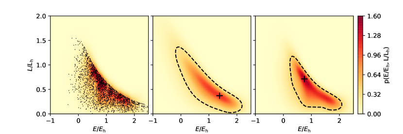
Figure 4: Phase-space distribution of subhalos for template halo A1. The discrete distribution in the left panel is taken directly from the simulations. The smooth distribution in the middle panel includes the fiducial measurement errors. The right panel assumes $\sigma_{\mu_{\alpha}}=\sigma_{\mu_{\delta}}=0.01\ \mathrm{mas\,yr}^{-1}$ instead of the fiducial values of $0.08\ \mathrm{mas\,yr}^{-1}$ while all other errors remain the same as for the middle panel. Color indicates the probability density and the cross marks the point of the highest density. The dashed curves enclose the densest 68% of the region.

4 Tests with Mock Samples

In our method of halo mass determination, we scale a template halo of mass $M_{\mathrm{h}}$ to different masses and obtain a family of subhalo phase-space distributions $p(E,L|M_{\mathrm{h}}^{\prime})$ following the procedure presented in Section 3. We then use these distributions and the $(E,L)$ data on the observed satellite tracers of a test halo to obtain the likelihood ${\cal L}({\rm obs}|M_{\mathrm{h}}^{\prime})$ as a function of $M_{\mathrm{h}}^{\prime}$ [see Equation (6)]. This gives the MLE $M_{\mathrm{esti}}$ for the test halo mass based on a specific set of scaled template halos. If the test halo is the MW, we will use the actual kinematic data on its dwarf satellite galaxies. For each satellite, the actual measurement errors will be used to make mock observations to obtain the corresponding $p(E,L|M_{\mathrm{h}}^{\prime})$ while the central values of the kinematic data in HSR will be used (along with the central values of the solar position and velocities relative to the GC) to obtain the corresponding $(E,L)$ in GSR. To test the validity and accuracy of our method, we choose a subset from the subhalos of a template halo to serve as the “observed” satellite tracers. These tracers are referred to as the mock sample and their $(E,L)$ data are obtained by making a single mock observation of each tracer as described in Section 3.4. Below we present a series of tests of our method using these mock samples.

4.1 Bias in the MLE for a specific template halo

We first check how well the true mass $M_{\mathrm{true}}$ of a halo can be recovered by the MLE $M_{\mathrm{esti}}$ in our method. As an example, we use template halo A1 as both the test halo to generate mock samples and the template to estimate the mass of the test halo. We randomly pick 9 of its subhalos to make a mock sample and apply our method to obtain the corresponding $M_{\mathrm{esti}}$. We repeat this with 5000 random mock samples to obtain a distribution of $M_{\mathrm{esti}}/M_{\mathrm{true}}$ at $M_{\mathrm{true}}=1.58\times 10^{12}M_{\odot}$ for template halo A1. We then use halos scaled from template halo A1 as test halos and obtain distributions of $M_{\mathrm{esti}}/M_{\mathrm{true}}$ for $M_{\mathrm{true}}=(0.5$–$3.0)\times 10^{12}M_{\odot}$. We find that to very good approximation, all these distributions can be fitted to a single Gaussian $\mathcal{N}(0.83,0.26^{2})$ with a mean of 0.83 and a standard deviation of 0.26. This is illustrated by the excellent agreement between the histograms showing the distributions for $M_{\mathrm{true}}=(0.5,1,2)\times 10^{12}M_{\odot}$ and the dashed curve for the Gaussian fit in the right panel of Figure 5. In addition, the left panel of this figure shows the median value (solid curve) and the 68% ($1\sigma$, dashed curves) and 95% ($2\sigma$, dot-dashed curves) intervals for $M_{\mathrm{esti}}/M_{\mathrm{true}}$ as functions of $M_{\mathrm{true}}$. These again agree very well with the Gaussian fit.

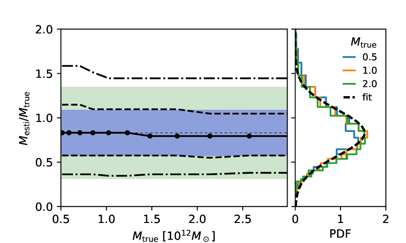
Figure 5: Distribution of $M_{\mathrm{esti}}/M_{\mathrm{true}}$ as a function of $M_{\mathrm{true}}$ for test halos scaled from template halo A1. Left panel: The solid, dashed, dot-dashed curves show the median value and the 68% ($1\sigma$) and 95% ($2\sigma$) intervals for $M_{\mathrm{esti}}/M_{\mathrm{true}}$ as functions of $M_{\mathrm{true}}$, which agree very well with the corresponding characteristics of the Gaussian distribution $\mathcal{N}(0.83,0.26^{2})$ (thin dotted line and shaded regions). Right panel: The histograms show the distributions of $M_{\mathrm{esti}}/M_{\mathrm{true}}$ for $M_{\mathrm{true}}=(0.5,1,2)\times 10^{12}M_{\odot}$, which are in excellent agreement with the dashed curve showing the Gaussian distribution.

As Figure 5 shows, the MLE $M_{\mathrm{esti}}$ tends to underestimate the halo mass $M_{\mathrm{true}}$ with a bias that is nearly independent of $M_{\mathrm{true}}$. Recall that the likelihood is constructed from the phase-space distribution $p(E,L|M_{\mathrm{h}}^{\prime})$ as a function of $M_{\mathrm{h}}^{\prime}$. Because $E$ also depends on $M_{\mathrm{h}}^{\prime}$, the likelihood is non-Bayesian and gives a biased MLE. As shown in Figure 1, $p(E,L|M_{\mathrm{h}}^{\prime})$ is denser for a lower $M_{\mathrm{h}}^{\prime}$. Thus the likelihood tends to favor a smaller halo mass than the true value. This bias is intrinsic to our method, but as shown below, it is insensitive to the number of tracers used, the measurement errors, or the formation history of the halo. Therefore, we can use $\hat{M}_{\mathrm{esti}}=M_{\mathrm{esti}}/\eta$ with $\eta=\langle M_{\mathrm{esti}}/M_{\mathrm{true}}\rangle=0.83$ as an essentially unbiased estimator for the halo mass. However, the relative uncertainty of $\hat{M}_{\mathrm{esti}}$ depends on the number of tracers used and the measurement errors, being $\sim 30\%$ for 9 tracers with the fiducial measurement errors.

Using template halo A1 as the test halo, we show in Figure 6 the distributions of $\hat{M}_{\mathrm{esti}}/M_{\mathrm{true}}$ for different numbers ($N$) of tracers and observational errors. We take $N=9$, 50, and 400, respectively. As proper-motion measurements dominate the observational uncertainties, we take $\sigma_{\mu_{\alpha}}=\sigma_{\mu_{\delta}}=0.08$, 0.03, and 0.01 $\mathrm{mas\,yr}^{-1}$, respectively, but keep the other measurement errors at their fiducial values. For each choice of $(N,\sigma_{\mu_{\alpha,\delta}})$, the distribution of $\hat{M}_{\mathrm{esti}}/M_{\mathrm{true}}$ (histogram) can be well fitted by a Gaussian (red curve) centered at $\hat{M}_{\mathrm{esti}}/M_{\mathrm{true}}=1$ with the standard deviation (“std”) indicated in the corresponding panel of Figure 6. This demonstrates that the fixed bias-correction $\eta=0.83$ works quite well for very different numbers of tracers and measurement errors. As shown in Figure 6, the standard deviation of $\hat{M}_{\mathrm{esti}}/M_{\mathrm{true}}$ decreases when more tracers and more precise observations are used. For fixed measurement errors, this quantity exhibits the expected $1/\sqrt{N}$ dependence.

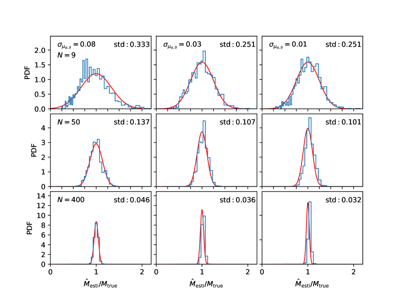
Figure 6: Distributions of $\hat{M}_{\mathrm{esti}}/M_{\mathrm{true}}$ for different numbers ($N$) of tracers and observational errors ($\sigma_{\mu_{\alpha,\delta}}$) when template halo A1 is used as the test halo. The upper, middle, and lower rows assume $N=9$, 50, and 400, respectively. The left, middle, and right columns assume $\sigma_{\mu_{\alpha,\delta}}=0.08$, 0.03, and 0.01 $\mathrm{mas\,yr}^{-1}$, respectively. In each case, the histogram showing the distribution can be well described by the red curve showing a Gaussian centered at $\hat{M}_{\mathrm{esti}}/M_{\mathrm{true}}=1$ with the standard deviation (“std”) indicated in the corresponding panel.

We have also checked that the corrected halo-mass estimator $\hat{M}_{\mathrm{esti}}=M_{\mathrm{esti}}/\eta$ with $\eta=0.83$ works consistently when each of the 9 template halos is used as both the test halo and the template to estimate the test halo mass. Figure 7 shows the distribution of $\hat{M}_{\mathrm{esti}}/M_{\mathrm{true}}$ in each case when the mock samples are observed with the fiducial measurement errors. All the distributions can again be well fitted by a Gaussian $\mathcal{N}(1,0.3^{2})$. While the median value of $\hat{M}_{\mathrm{esti}}/M_{\mathrm{true}}$ fluctuates slightly around unity, this fluctuation is $<5\%$, well within the standard deviation. Therefore, $\hat{M}_{\mathrm{esti}}$ recovers the true halo mass within $\sim 30\%$ for all the 9 template halos used as test halos. Because these halos have very different formation history and dynamical status, this demonstrates the validity and robustness of our method at least when the formation history of a test halo is known.

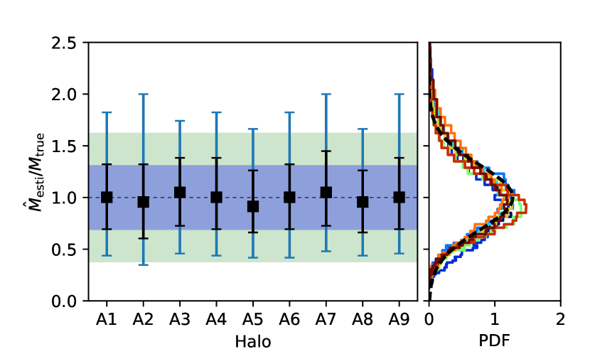
Figure 7: Distribution of $\hat{M}_{\mathrm{esti}}/M_{\mathrm{true}}$ when each of the 9 template halos is used as the test halo. Left panel: The filled squares and error bars show the median value and the 68% ($1\sigma$) and 95% ($2\sigma$) intervals for $\hat{M}_{\mathrm{esti}}/M_{\mathrm{true}}$. These compare very well with the thin dotted line and the shaded regions showing the corresponding characteristics of the Gaussian distribution $\mathcal{N}(1,0.3^{2})$. Right panel: The histograms showing the distributions of $\hat{M}_{\mathrm{esti}}/M_{\mathrm{true}}$ are compared with the dashed curve showing the Gaussian distribution.

4.2 Influence of subhalo mass

Our method implicitly assumes that the phase-space distribution of subhalos is independent of their masses. This is supported by recent studies (e.g. Han et al., 2016a), which showed that small and massive subhalos have very similar dynamics. This can be understood because dynamical friction with strong mass dependence is important only for major mergers. Nevertheless, because the intended tracers for the MW halo are its satellite galaxies, the more luminous of which tend to inhabit massive subhalos, we carry out further tests to check any possible influence of subhalo mass on our method.

In the first test, we scale each of the 9 template halos to a mass of $M_{\mathrm{true}}=1.5\times 10^{12}M_{\odot}$ and take the most massive (at infall) 9 subhalos in each case as the mock sample with the fiducial measurement errors. Figure 8 shows $\hat{M}_{\mathrm{esti}}/M_{\mathrm{true}}$ (filled squares) for these test halos. These results are fully consistent with those in Figure 7, which are obtained from mock samples each having 9 randomly-selected subhalos. Specifically, when the results in Figure 8 are compared with the Gaussian distribution $\mathcal{N}(1,0.3^{2})$, the $\chi^{2}$ test gives $P(>\chi^{2})=0.46$, which indicates no deviation. This insensitivity to the mock sample is also confirmed when we scale the template halos to other masses and use those as test halos.

Figure 8: Results obtained from mock samples each having the most massive 9 subhalos of a halo. The filled squares give the $\hat{M}_{\mathrm{esti}}/M_{\mathrm{true}}$ when each of the template halos is scaled to $M_{\mathrm{true}}=1.5\times 10^{12}M_{\odot}$ and used as the test halo. The thin dotted line and the shaded regions show the median and the $1\sigma$ and $2\sigma$ intervals for the Gaussian distribution $\mathcal{N}(1,0.3^{2})$. The p-value of the $\chi^{2}$ test of the filled squares against the Gaussian distribution is $P(>\chi^{2})=0.46$.

In the second test, mock samples are created by randomly selecting 9 subhalos from the top 100 massive subhalos in each of the 9 template halos used as test halos. We show in Figure 9 the distribution of $\hat{M}_{\mathrm{esti}}/M_{\mathrm{true}}$ obtained from 5000 mock samples for each test halo. These results are almost the same as those in Figure 7.

Based on the above tests and in view of the $\sim 30\%$ uncertainty in our halo mass estimate, which is mostly due to the relatively small number of tracers used and the rather significant errors in proper motion measurement, we conclude that any influence of subhalo mass can be safely ignored. In any case, when the number of the MW satellite galaxies with precise kinematic data increases, this sample will reach tracers of lower luminosity associated with less massive subhalos, and therefore, become closer to a sample of randomly-selected subhalo tracers best suited for our method.

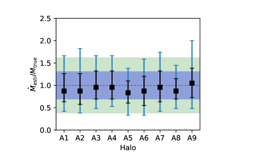
Figure 9: Same as the left panel of Figure 7, but the mock samples are randomly drawn from the top 100 massive subhalos in each test halo.

4.3 Halo-to-halo scatter

So far we have shown that if the formation history of a test halo is known, the halo mass can be determined reliably by our method. However, halo formation history is not readily available in practice. Without such information, we must resort to comparing the kinematic data on the observed tracers of a test halo with the subhalo phase-space distributions for a number of template halos with a wide range of formation history. For example, when we use template halo A1 as the test halo, we estimate its mass using all the 9 template halos. For clarity, we refer to template halo A1 in this case as test halo A1. Figure 10 shows the distributions of $\hat{M}_{\mathrm{esti}}/M_{\mathrm{true}}$ for test halo A1 obtained by comparing fiducial mock samples (9 tracers with fiducial measurement errors) from this halo with the phase-space distribution from each of the 9 template halos. The influence of halo formation history on $\hat{M}_{\mathrm{esti}}/M_{\mathrm{true}}$ can be seen clearly.

Figure 10: Distribution of $\hat{M}_{\mathrm{esti}}/M_{\mathrm{true}}$ obtained for test halo A1 by comparing mock samples from this halo with each of the 9 template halos. Left panel: The filled squares and error bars show the median value and the 68% and 95% intervals of $\hat{M}_{\mathrm{esti}}/M_{\mathrm{true}}$. The thin dotted line and the shaded regions indicate a Gaussian distribution centered at unity with a standard deviation of 0.3. The rightmost filled square with error bars shows $\hat{\overline{M}}_{\mathrm{esti}}/M_{\mathrm{true}}$ obtained by averaging the results from all 9 template halos. Right panel: The distribution of $\hat{\overline{M}}_{\mathrm{esti}}/M_{\mathrm{true}}$ is compared with a lognormal $\ln\mathcal{N}(0,0.35^{2})$.

To address the lack of the formation history of a test halo, we take the average of the $\hat{M}_{\mathrm{esti}}$ obtained for this halo using the subhalo phase-space distribution for each of the template halos,

$$\hat{\overline{M}}_{\mathrm{esti}}=\sum_{i=1}^{N_{\rm temp}}\frac{\hat{M}_{\mathrm{esti}}\phantom{}{}_{,i}}{N_{\rm temp}},$$ (19)

and check if this average (for $N_{\rm temp}=9$) gives a better estimate. We show the distribution of $\hat{\overline{M}}_{\mathrm{esti}}/M_{\mathrm{true}}$ for test halo A1 in Figure 10. The rightmost filled square in this figure shows that the median $\hat{\overline{M}}_{\mathrm{esti}}/M_{\mathrm{true}}$ is 1. On the other hand, the corresponding 68% and 95% intervals are asymmetric and favor higher values. As shown in the right panel of Figure 10, the distribution of $\hat{\overline{M}}_{\mathrm{esti}}/M_{\mathrm{true}}$ is well described by a lognormal $\ln\mathcal{N}(0,0.35^{2})$. Using other template halos as test halos, we show in Figure 11 the corresponding distributions of $\hat{\overline{M}}_{\mathrm{esti}}/M_{\mathrm{true}}$. The filled squares with error bars in the left panel show the median value and the 68% and 95% intervals of $\hat{\overline{M}}_{\mathrm{esti}}/M_{\mathrm{true}}$ for each test halo. The median $\hat{\overline{M}}_{\mathrm{esti}}/M_{\mathrm{true}}$ scatters around unity within $\sim 20\%$ ($\sim 30\%$ for a few cases), reflecting the difference in formation history between the test and template halos. We have also checked that the bias of $\hat{\overline{M}}_{\mathrm{esti}}/M_{\mathrm{true}}$ does not depend on the number of tracers used or the measurement errors (not shown). Note that the relative uncertainty in $\hat{\overline{M}}_{\mathrm{esti}}/M_{\mathrm{true}}$ is $\sim 30\%$ for all 9 test halos.

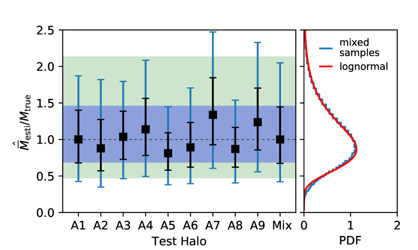
Figure 11: Distribution of $\hat{\overline{M}}_{\mathrm{esti}}/M_{\mathrm{true}}$ for each test halo. Left panel: The filled squares and error bars show the median value and the 68% and 95% intervals for $\hat{\overline{M}}_{\mathrm{esti}}/M_{\mathrm{true}}$. The thin dotted line and the shaded regions show the median and the $1\sigma$ and $2\sigma$ intervals for the lognormal distribution $\ln\mathcal{N}(0,0.38^{2})$. The rightmost filled square with error bars shows the result for the mixed mock samples randomly drawn from the 9 test halos. Right panel: The distribution of $\hat{\overline{M}}_{\mathrm{esti}}/M_{\mathrm{true}}$ for the mixed mock samples is compared with the lognormal distribution.

As a final test, we make mock samples by randomly picking a test halo and then randomly selecting 9 subhalos from this halo. Based on 5000 such mixed mock samples, we show the distribution of $\hat{\overline{M}}_{\mathrm{esti}}/M_{\mathrm{true}}$ as the rightmost filled square with error bars (left panel) and the histogram (right panel) in Figure 11. This distribution best characterizes the halo mass estimate given by our method in practice, and is well described by a lognormal $\ln\mathcal{N}(0,0.38^{2})$, whose $1\sigma$ interval corresponds to the interval $[0.68,1.46]$ for $\hat{\overline{M}}_{\mathrm{esti}}/M_{\mathrm{true}}$. The uncertainty is slightly larger than the case with mock samples from a single test halo because a discrepancy of $\sim 20\%$ due to halo-to-halo scatter is also included in addition to the statistical uncertainty. More precisely, the uncertainty due to halo-to-halo scatter is $19_{-4}^{+6}\%$ based on the variance of the 9 data points in Figure 11. While this uncertainty is irreducible without additoinal information, it can be estimated better with more test halos. In addition, the limited number (9) of template halos also introduces an uncertainty of $\sim 20\%/\sqrt{9}\approx 7\%$ in $\hat{\overline{M}}_{\mathrm{esti}}/M_{\mathrm{true}}$. However, this uncertainty is relatively small compared to that from halo-to-halo scatter.

In principle, knowledge on the formation history of a test halo can reduce the uncertainty in its mass estimate due to halo-to-halo scatter. Of particular importance is information on the growth of the halo potential as well as the accretion and disruption of substructures. However, it is difficult to find a simple indicator to characterize the influence of the halo assembly history on the kinematics of surviving substructures. We intend to study this problem in the future.

4.4 Prospects and limitation

Based on the preceding discussion, there are two main sources of uncertainties in our method of halo mass determination: one is statistical and due to the limited number of tracers and measurement errors, while the other is intrinsic and due to the lack of knowledge about the formation history of a test halo. Below we quantify these uncertainties using mixed mock samples created by randomly picking one of the test halos and then randomly selecting a subset of its subhalos. We vary the sample size (the number $N$ of tracers) and the error $\sigma_{\mu}=\sigma_{\mu_{\alpha}}=\sigma_{\mu_{\delta}}$ in proper motion measurement, which dominates the observational uncertainties. The other measurement errors are kept at their fiducial values.

Because $\hat{\overline{M}}_{\mathrm{esti}}/M_{\mathrm{true}}$ follows a lognormal distribution, we define the uncertainty of our method as

$$\sigma=\sqrt{\mathrm{var}\left[\ln\left(\hat{\overline{M}}_{\mathrm{esti}}/M_{\mathrm{true}}\right)\right]}\,.$$ (20)

Note $\mathrm{var}(X)\simeq\mathrm{var}(\ln X)$ when $X$ follows $\ln\mathcal{N}(0,\sigma^{2})$ and $\sigma$ is small.

In Figure 12, we show $\sigma$ as a function of the number $N$ of tracers for $\sigma_{\mu}=0.01$, 0.03, 0.06, and 0.08 $\mathrm{mas\,yr}^{-1}$, respectively. As shown by the dashed curves, these results can be well described by

$$\sigma^{2}=\sigma_{\mathrm{stat}}^{2}+\sigma_{\mathrm{hist}}^{2}=\frac{A^{2}\sigma_{\mu}^{2}+\sigma_{\mathrm{other}}^{2}}{N}+\sigma_{\mathrm{hist}}^{2},$$ (21)

where $\sigma_{\mathrm{stat}}$ is the statistical term that decreases with increasing $N$, and $\sigma_{\mathrm{hist}}$ is the intrinsic term due to the lack of knowledge about the halo formation history. The statistical term can be specified by $A\sigma_{\mu}$, where $A$ is a constant, and $\sigma_{\mathrm{other}}$, which captures the other observational uncertainties and errors in constructing the subhalo phase-space distribution. Fit to the data gives $A=8.75$, $\sigma_{\mathrm{other}}=0.80$, and $\sigma_{\mathrm{hist}}=0.17$. Note that $\sigma_{\mathrm{hist}}$ depends on the template halos used and may be estimated better with more halos in addition to the 9 used here.

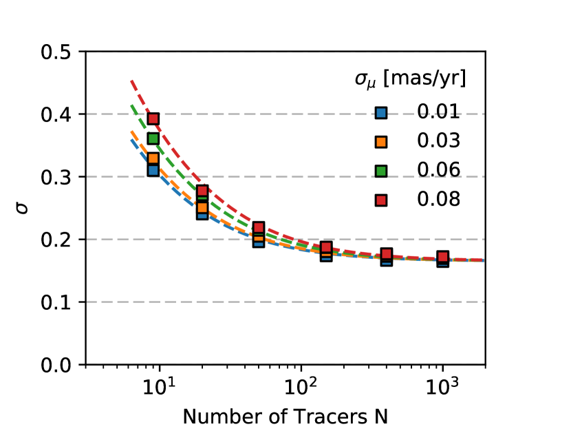
Figure 12: Uncertainty $\sigma$ in $\ln\left(\hat{\overline{M}}_{\mathrm{esti}}/M_{\mathrm{true}}\right)$ as a function of the number $N$ of tracers for different values of the error $\sigma_{\mu}$ in proper motion measurement. Filled squares are data obtained using mixed mock samples randomly drawn from the 9 test halos. Good fit to the data is provided by the dashed curves for $\sigma^{2}=(8.75^{2}\sigma_{\mu}^{2}+0.80^{2})/N+0.17^{2}$.

For the fiducial number of tracers ($N=9$) with the fiducial measurement errors ($\sigma_{\mu}=0.08\ \mathrm{mas\,yr}^{-1}$), $\sigma$ is $\sim 40\%$. If $N$ increases to 30, $\sigma$ decreases to $\sim$25% for the fiducial measurement precision. However, as $N$ increases further, $\sigma$ becomes dominated by $\sigma_{\mathrm{hist}}$. This sets a limiting number of tracers at $N\sim 50$, beyond which there is no significant gain in the accuracy of our halo mass estimate. This is similar to the result of Wang et al. (2016), who gave a systematic uncertainty of 25–40% for the MW mass estimate using dynamical tracers under the steady-state assumption. We emphasize that the ultimate improvement of our method requires detailed knowledge about the formation history of a test halo.

5 Conclusions

We have presented a method to estimate the mass of a dark matter halo using the kinematic data of its subhalo tracers, which are satellite galaxies in practice. The halo mass is inferred by comparing these data with the distribution in the phase space of binding energy and angular momentum for subhalos in each of the template halos obtained in cosmological simulations. We have tested the validity and accuracy of this method with mock samples and found that the halo mass can be recovered within $\sim 40\%$ by using 9 tracers with the current observational precision. The uncertainty can be reduced to $\sim$25% if the number of tracers with sufficiently accurate proper motion measurement increases to 30 in the future. However, the subhalo phase-space distribution depends on the halo formation history and the lack of this knowledge results in an intrinsic uncertainty of $\sim 20$% in our halo mass estimate, which cannot be reduced by increasing the number of tracers. Further studies on the assembly history of a halo and how this history affects the kinematics of its substructures are essential to an accurate determination of its mass. A direct application of our method is to estimate the mass of the MW halo. Using the data on its 9 dwarf satellite galaxies, we obtain a mass of $1.3\times 10^{12}M_{\odot}$ with uncertainties comparable to the expected value of $\sim 40\%$. This preliminary result is consistent with various estimates in the literature. A detailed report will be given elsewhere.

Although they do not seem to affect our current results, several issues regarding our approach merit discussion. We have found that the phase-space distribution is nearly independent of subhalo mass. Because satellite galaxies are the intended subhalo tracers, it is desirable to confirm this with further tests using satellite samples from semi-analytical or hydrodynamic simulations. We have simulated 9 template halos with a wide range of formation history. It is valuable to have more template halos to check if this range is sufficiently representative. Because high-resolution zoom-in simulations are required to provide well-resolved substructures for constructing the phase-space distributions, it is computationally intensive to study many template halos. Another issue is the influence of massive neighbors such as M31 in the case of the MW. Our 9 template halos are chosen to be relatively isolated to exclude such neighbors. Using a larger halo sample, we have checked that the presence of a massive neighbor will not affect our method when the distance to the neighbor exceeds three times its virial radius as in the case of M31 and the MW (see Appendix). Finally, in our mock observations, we set the origin of the “GSR” to rest at the center of a template halo. However, theoretical and observational studies suggest that central galaxies do not necessarily rest at the centers of their host halos (e.g. Berlind et al., 2003; Yoshikawa et al., 2003). A recent study by Guo et al. (2015) reported that a central galaxy tends to move around the host halo center with a dispersion of $0.2\sigma_{v,\mathrm{DM}}$ ($\sim 30\ \mathrm{km\,s}^{-1}$ for the MW) for each velocity component. In addition, if the LMC exceeds 10% of the MW mass, then the MW is moving relative to their barycenter at a velocity of $\sim 30\ \mathrm{km\,s}^{-1}$ ($v_{\mathrm{LMC}}\simeq 300\ \mathrm{km\,s}^{-1}$ relative to the GC). In principle, the unknown velocity offset between the GC and the MW halo center introduces an extra uncertainty in the MW halo mass estimate. However, in practice, we find with Monte Carlo experiments that adding an extra velocity of 30 $\mathrm{km\,s}^{-1}$ to the “GC” in mock observations only changes the results at the $\lesssim 3\%$ level. So this effect might become significant only when the intrinsic uncertainty in our method is reduced with information on the halo formation history.

Currently, our method is still limited by the number of tracers and measurement errors. Proper motions are only available for 12 of the 13 MW satellite galaxies (the exception being Canes Venatici I) that are more luminous than $10^{5}L_{\odot}$ and within 300 kpc of the GC. The best of these proper motion measurements were made with HST. The Gaia mission will reduce uncertainties in proper motions of nearby classical satellites (e.g. van der Marel & Sahlmann, 2016) and make new measurements for fainter objects within $\sim$100 kpc of the Sun (Wilkinson & Evans, 1999). Proper motions of more distant satellite galaxies could be measured by a multi-year HST program with followup by the James Webb Space Telescope (JWST) or the Wide-Field Infrared Survey Telescope (WFIRST) (Kallivayalil et al., 2015). In addition, ongoing deep, wide-field sky surveys, such as the Dark Energy Survey (DES), PanSTARRS 1 (PS1), and VST ATLAS have doubled the number of known MW satellites over the past two years (e.g Bechtol et al., 2015; Koposov et al., 2015; Drlica-Wagner et al., 2015; Laevens et al., 2015; Torrealba et al., 2016). The number of satellites brighter than the faintest known dwarf galaxies might eventually reach 300–600 and possibly as high as $\sim$1000 (Tollerud et al., 2008). The above exciting progress in observations will undoubtedly enable us to determine the MW halo mass with increasing accuracy.

Validation with more test halos from cosmological simulations

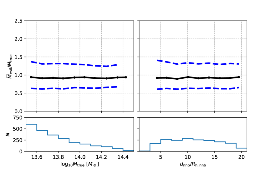
Figure 13: Distribution of $\overline{M}_{\mathrm{esti}}/M_{\mathrm{true}}$ (upper panels) and number of test halos $N$ (lower panels) as functions of the true halo mass $M_{\mathrm{true}}$ (left panels) and the distance to the nearest more massive neighbor relative to its halo radius $d_{\rm nnb}/R_{\rm h,nnb}$ (right panels) for a sample of test halos from cosmological simulations. The solid and dashed curves in upper panels show the median value and the 68% ($1\sigma$) intervals for $\overline{M}_{\mathrm{esti}}/M_{\mathrm{true}}$ in a bin of $M_{\mathrm{true}}$ (left panel) and $d_{\rm nnb}/R_{\rm h,nnb}$ (right panel). The histograms in lower panels show the number of test halos in each bin.

Our method recovers the true halo mass consistently in a series of tests with the 9 halos from zoom-in simulations. Nevertheless, it is important to check the robustness of the method with a larger test halo sample. Such a sample can also be used to investigate how a massive neighbor may affect the mass estimate for a halo, thereby checking the validity of using relatively isolated template halos in our method. We select a set of test halos from 6 cosmological simulations. Each simulation was performed with $1024^{3}$ particles in a periodic cubic box of $(150h^{-1}\,\mathrm{Mpc})^{3}$. A $\Lambda\mathrm{CDM}$ cosmology was adopted with $\Omega_{m}=0.268$, $\Omega_{\Lambda}=0.732$, $h=0.71$, $n_{s}=1$, and $\sigma_{8}=0.85$ (Jing et al., 2007). The particle mass in these simulations is $2.3\times 10^{8}h^{-1}\,M_{\odot}$. We identify halos and subhalos in the same way as described in Section 3.1. We note that the cosmological parameters adopted above are somewhat different from those in the main text. We expect that the effect of this difference would be small compared to that of the difference in halo formation history for application of our method.

To ensure a sufficient number of well-resolved subhalos in each test halo, we focus on halos in the mass range of $\sim 2\times(10^{13}$–$10^{14})h^{-1}\,M_{\odot}$ and obtain a sample of 2681 test halos. For each test halo, we select subhalos with a maximum binding mass of $m_{\rm max}>300$ particles over history, a mass of $m_{0}>10$ particles at present, and a distance of $160\ \mathrm{kpc}<r<1200\ \mathrm{kpc}$ to the halo center. We then randomly pick 9 subhalos to make a mock sample. (For the least massive halos, which amount to $<1.5\%$ of the test halo sample and contain fewer than 9 usable subhalos each, we randomly pick 9 subhalos with repetition.) Mock observations of the 9 subhalos are made with measurement errors $\sigma_{r}/r=0.06$, $\sigma_{v_{\mathrm{los}}}=4\ \mathrm{km\,s}^{-1}$, and $\sigma_{\mu}=0.08\ \mathrm{mas\,yr}^{-1}$. The above numerical values are the same as in Section 3, except that the distance range and $\sigma_{v_{\mathrm{los}}}$ are increased in proportion to the mass range of the test halos under consideration. Following the procedure in Section 3, we estimate the mass of a test halo by comparing the phase space distribution of its mock sample with those of a template halo scaled to the same mass range. The results using the 9 template halos A1–A9 are averaged to calculate the final estimate $\overline{M}_{\mathrm{esti}}$.

A total of 20 mock samples are chosen from each test halo to generate a distribution of $\overline{M}_{\mathrm{esti}}/M_{\mathrm{true}}$, where $M_{\mathrm{true}}$ is the true halo mass. This distribution is shown in the upper left panel of Figure 13 as a function of $M_{\mathrm{true}}$ for the entire test halo sample. The solid and dashed curves give the median value and the 68% ($1\sigma$) intervals, respectively, for the $\overline{M}_{\mathrm{esti}}/M_{\mathrm{true}}$ of all the mock samples in a bin of $M_{\mathrm{true}}$. The number of test halos in each bin is shown in the lower left panel of Figure 13. It can be seen that although the test halos [$\sim 3\times(10^{13}$–$10^{14})M_{\odot}$] have very different masses from the template halos ($\sim 1.5\times 10^{12}M_{\odot}$), our method still gives reasonable mass estimates. The median value of $\overline{M}_{\mathrm{esti}}/M_{\mathrm{true}}$ is nearly independent of $M_{\mathrm{true}}$ and can be taken as the bias $\eta=0.92$. In addition, the uncertainty of $\overline{M}_{\mathrm{esti}}/M_{\mathrm{true}}$ also has little dependence on $M_{\mathrm{true}}$. These results are similar to those shown in Figure 5 for MW-like test halos and demonstrate that our method using scaled templates is valid for a fixed range with a factor of $\sim 6$ variation in the halo mass even when these masses differ greatly from those for the template halos.

The distribution of $\overline{M}_{\mathrm{esti}}/M_{\mathrm{true}}$ shown in Figure 13 can be well described by a lognormal with $\sigma=0.4$ [see similar definition in Equation (20)], which extends the results in Section 4.4 to much larger halo masses. However, the bias $\eta=0.92$ is $\approx 10\%$ larger than the value of 0.83 adopted for MW-like halos. This small difference may be due to the difference in assembly history between MW-like halos and the test halos under consideration, with possibly a minor contribution from the somewhat different cosmology adopted for the template and test halos. It is also possible that the template halos A1–A9 are not representative enough. While we cannot identify the exact cause for the above difference in $\eta$, we note that this issue is secondary compared to the $\sim 40\%$ overall uncertainty of our method when applied to the MW with the current observational constraints. However, in anticipation of major improvement of observations, more detailed investigation with many more template halos is required to better understand the influence of halo assembly history on our method.

For each of our template halos, its distance to any more massive halo exceeds three times the sum of the virial radii of both halos. We now investigate how this choice of relatively isolated template halos may influence the mass estimate. Satellites of a halo are subject to both the gravitational force of the halo and the tidal force of a massive neighbor. For a halo of mass $M_{\mathrm{h}}$ and virial radius $R_{\mathrm{h}}$ with a neighbor of mass $M_{\rm nb}$ and virial radius $R_{\rm h,nb}$ at a distance $d_{\rm nb}$, the gravitational force of the halo on a satellite of mass $m_{\rm sat}$ is $F_{\textrm{g}}\sim GM_{\mathrm{h}}m_{\rm sat}/R_{\mathrm{h}}^{2}$, while the tidal force of the neighbor is $F_{\rm t}\sim GM_{\rm nb}m_{\rm sat}R_{\mathrm{h}}/d_{\rm nb}^{3}$. So the importance of the neighbor can be gauged by $F_{\rm t}/F_{\rm g}\sim(M_{\rm nb}/M_{\mathrm{h}})(R_{\mathrm{h}}/d_{\rm nb})^{3}$. Because the halo and its neighbor have the same average density, $M_{\rm nb}/R_{\rm h,nb}^{3}=M_{\mathrm{h}}/R_{\mathrm{h}}^{3}$, we obtain $F_{\rm t}/F_{\rm g}\sim(R_{\rm h,nb}/d_{\rm nb})^{3}$. Using the sample of test halos from cosmological simulations, we locate every more massive halo in the neighborhood of a test halo and define the one with the smallest $d_{\rm nb}/R_{\rm h,nb}$ as the nearest neighbor. As shown in the upper right panel of Figure 13, the mass estimate is essentially independent of $d_{\rm nnb}/R_{\rm h,nnb}$ for $d_{\rm nnb}/R_{\rm h,nnb}\gtrsim 3$. Therefore, it is appropriate to use our template halos with $d_{\rm nnb}/(R_{\rm h,nnb}+R_{\mathrm{h}})>3$ to estimate the masses of those halos with $d_{\rm nnb}/R_{\rm h,nnb}\gtrsim 3$. The galaxy M31 is perhaps slightly more massive than the MW and is at a distance of $d_{\rm M31}\sim 800\ \mathrm{kpc}$. The virial radius of its dark matter halo can be estimated as $R_{\rm M31}\sim 200\ \mathrm{kpc}$. With $d_{\rm M31}/R_{\rm M31}\sim 4$, the effect of the tidal force of M31 is at the level of $\sim 2\%$ and our method can be safely applied to estimate the mass of the MW halo.

References

- Arvo (1992) Arvo, J. 1992, in Graphics Gems III, ed. D. Kirk (San Diego, CA, USA: Academic Press Professional, Inc.), 117–120. http://dl.acm.org/citation.cfm?id=130745.130767
- Astropy Collaboration et al. (2013) Astropy Collaboration, Robitaille, T. P., Tollerud, E. J., et al. 2013, Astronomy and Astrophysics, 558, A33. http://adsabs.harvard.edu/abs/2013A%26A...558A..33A
- Banik & Zhao (2016) Banik, I., & Zhao, H. 2016, Monthly Notices of the Royal Astronomical Society, 459, 2237. http://adsabs.harvard.edu/abs/2016MNRAS.459.2237B
- Barber et al. (2014) Barber, C., Starkenburg, E., Navarro, J. F., McConnachie, A. W., & Fattahi, A. 2014, Monthly Notices of the Royal Astronomical Society, 437, 959. http://adsabs.harvard.edu/abs/2014MNRAS.437..959B
- Bechtol et al. (2015) Bechtol, K., Drlica-Wagner, A., Balbinot, E., et al. 2015, The Astrophysical Journal, 807, 50. http://adsabs.harvard.edu/abs/2015ApJ...807...50B
- Berlind et al. (2003) Berlind, A. A., Weinberg, D. H., Benson, A. J., et al. 2003, The Astrophysical Journal, 593, 1. http://adsabs.harvard.edu/abs/2003ApJ...593....1B
- Bland-Hawthorn & Gerhard (2016) Bland-Hawthorn, J., & Gerhard, O. 2016, Annual Review of Astronomy and Astrophysics, 54, 529. http://adsabs.harvard.edu/abs/2016ARA%26A..54..529B
- Boylan-Kolchin et al. (2011) Boylan-Kolchin, M., Bullock, J. S., & Kaplinghat, M. 2011, Monthly Notices of the Royal Astronomical Society: Letters, 415, L40. http://arxiv.org/abs/1103.0007
- Boylan-Kolchin et al. (2013) Boylan-Kolchin, M., Bullock, J. S., Sohn, S. T., Besla, G., & van der Marel, R. P. 2013, The Astrophysical Journal, 768, 140. http://adsabs.harvard.edu/abs/2013ApJ...768..140B
- Cautun et al. (2014) Cautun, M., Wang, W., Frenk, C. S., & Sawala, T. 2014, arXiv:1410.7778 [astro-ph], arXiv:1410.7778. http://arxiv.org/abs/1410.7778
- Courteau et al. (2014) Courteau, S., Cappellari, M., de Jong, R. S., et al. 2014, Reviews of Modern Physics, 86, 47. http://adsabs.harvard.edu/abs/2014RvMP...86...47C
- Drlica-Wagner et al. (2015) Drlica-Wagner, A., Bechtol, K., Rykoff, E. S., et al. 2015, The Astrophysical Journal, 813, 109. http://adsabs.harvard.edu/abs/2015ApJ...813..109D
- Eadie et al. (2016) Eadie, G., Springford, A., & Harris, W. 2016, arXiv:1609.06304 [astro-ph], arXiv:1609.06304. http://arxiv.org/abs/1609.06304
- Eadie et al. (2015) Eadie, G. M., Harris, W. E., & Widrow, L. M. 2015, The Astrophysical Journal, 806, 54. http://adsabs.harvard.edu/abs/2015ApJ...806...54E
- Gibbons et al. (2014) Gibbons, S. L. J., Belokurov, V., & Evans, N. W. 2014, Monthly Notices of the Royal Astronomical Society, 445, 3788. http://adsabs.harvard.edu/abs/2014MNRAS.445.3788G
- Guo et al. (2015) Guo, H., Zheng, Z., Zehavi, I., et al. 2015, Monthly Notices of the Royal Astronomical Society, 446, 578. http://adsabs.harvard.edu/abs/2015MNRAS.446..578G
- Guo et al. (2011) Guo, Q., White, S., Boylan-Kolchin, M., et al. 2011, Monthly Notices of the Royal Astronomical Society, 413, 101. http://adsabs.harvard.edu/abs/2011MNRAS.413..101G
- Han et al. (2016a) Han, J., Cole, S., Frenk, C. S., & Jing, Y. 2016a, Monthly Notices of the Royal Astronomical Society, 457, 1208. http://arxiv.org/abs/1509.02175
- Han et al. (2012) Han, J., Jing, Y. P., Wang, H., & Wang, W. 2012, Monthly Notices of the Royal Astronomical Society, 427, 2437. http://adsabs.harvard.edu/abs/2012MNRAS.427.2437H
- Han et al. (2016b) Han, J., Wang, W., Cole, S., & Frenk, C. S. 2016b, Monthly Notices of the Royal Astronomical Society, 456, 1017. http://arxiv.org/abs/1507.00771
- Huang et al. (2016) Huang, Y., Liu, X., Yuan, H., et al. 2016, Monthly Notices of the Royal Astronomical Society, 463, 2623. http://arxiv.org/abs/1604.01216
- Jing & Suto (2000) Jing, Y. P., & Suto, Y. 2000, The Astrophysical Journal Letters, 529, L69. http://adsabs.harvard.edu/abs/2000ApJ...529L..69J
- Jing & Suto (2002) —. 2002, The Astrophysical Journal, 574, 538. http://iopscience.iop.org/0004-637X/574/2/538
- Jing et al. (2007) Jing, Y. P., Suto, Y., & Mo, H. J. 2007, The Astrophysical Journal, 657, 664. http://adsabs.harvard.edu/abs/2007ApJ...657..664J
- Kahn & Woltjer (1959) Kahn, F. D., & Woltjer, L. 1959, The Astrophysical Journal, 130, 705. http://adsabs.harvard.edu/abs/1959ApJ...130..705K
- Kallivayalil et al. (2015) Kallivayalil, N., Wetzel, A. R., Simon, J. D., et al. 2015, arXiv:1503.01785 [astro-ph], arXiv:1503.01785. http://arxiv.org/abs/1503.01785
- Koposov et al. (2015) Koposov, S. E., Belokurov, V., Torrealba, G., & Evans, N. W. 2015, The Astrophysical Journal, 805, 130. http://adsabs.harvard.edu/abs/2015ApJ...805..130K
- Laevens et al. (2015) Laevens, B. P. M., Martin, N. F., Ibata, R. A., et al. 2015, The Astrophysical Journal Letters, 802, L18. http://adsabs.harvard.edu/abs/2015ApJ...802L..18L
- Li & White (2008) Li, Y.-S., & White, S. D. M. 2008, Monthly Notices of the Royal Astronomical Society, 384, 1459. http://adsabs.harvard.edu/abs/2008MNRAS.384.1459L
- van der Marel & Sahlmann (2016) van der Marel, R. P., & Sahlmann, J. 2016, arXiv:1609.04395 [astro-ph], arXiv:1609.04395. http://arxiv.org/abs/1609.04395
- McConnachie (2012) McConnachie, A. W. 2012, The Astronomical Journal, 144, 4. http://adsabs.harvard.edu/abs/2012AJ....144....4M
- Pawlowski & Kroupa (2013) Pawlowski, M. S., & Kroupa, P. 2013, Monthly Notices of the Royal Astronomical Society, 435, 2116. http://adsabs.harvard.edu/abs/2013MNRAS.435.2116P
- Peñarrubia et al. (2016) Peñarrubia, J., Gómez, F. A., Besla, G., Erkal, D., & Ma, Y.-Z. 2016, Monthly Notices of the Royal Astronomical Society: Letters, 456, L54. http://arxiv.org/abs/1507.03594
- Piatek et al. (2005) Piatek, S., Pryor, C., Bristow, P., et al. 2005, The Astronomical Journal, 130, 95. http://adsabs.harvard.edu/abs/2005AJ....130...95P
- Piatek et al. (2003) Piatek, S., Pryor, C., Olszewski, E. W., et al. 2003, The Astronomical Journal, 126, 2346. http://adsabs.harvard.edu/abs/2003AJ....126.2346P
- Piatek et al. (2002) —. 2002, The Astronomical Journal, 124, 3198. http://adsabs.harvard.edu/abs/2002AJ....124.3198P
- Rodriguez-Puebla et al. (2013) Rodriguez-Puebla, A., Avila-Reese, V., & Drory, N. 2013, The Astrophysical Journal, 773, 172. http://arxiv.org/abs/1306.4328
- Springel (2005) Springel, V. 2005, Monthly Notices of the Royal Astronomical Society, 364, 1105. http://adsabs.harvard.edu/abs/2005MNRAS.364.1105S
- Starkenburg et al. (2013) Starkenburg, E., Helmi, A., De Lucia, G., et al. 2013, Monthly Notices of the Royal Astronomical Society, 429, 725. http://adsabs.harvard.edu/abs/2013MNRAS.429..725S
- Strigari et al. (2008) Strigari, L. E., Bullock, J. S., Kaplinghat, M., et al. 2008, Nature, 454, 1096. http://arxiv.org/abs/0808.3772
- Tollerud et al. (2008) Tollerud, E. J., Bullock, J. S., Strigari, L. E., & Willman, B. 2008, The Astrophysical Journal, 688, 277. http://adsabs.harvard.edu/abs/2008ApJ...688..277T
- Torrealba et al. (2016) Torrealba, G., Koposov, S. E., Belokurov, V., et al. 2016, Monthly Notices of the Royal Astronomical Society, 463, 712. http://adsabs.harvard.edu/abs/2016MNRAS.463..712T
- Wang et al. (2012) Wang, J., Frenk, C. S., Navarro, J. F., Gao, L., & Sawala, T. 2012, Monthly Notices of the Royal Astronomical Society, 424, 2715. http://arxiv.org/abs/1203.4097
- Wang et al. (2016) Wang, W., Han, J., Cole, S., Frenk, C., & Sawala, T. 2016, arXiv:1605.09386 [astro-ph], arXiv:1605.09386. http://arxiv.org/abs/1605.09386
- Wang et al. (2015) Wang, W., Han, J., Cooper, A. P., et al. 2015, Monthly Notices of the Royal Astronomical Society, 453, 377. http://adsabs.harvard.edu/abs/2015MNRAS.453..377W
- Watkins et al. (2010) Watkins, L. L., Evans, N. W., & An, J. H. 2010, Monthly Notices of the Royal Astronomical Society, 406, 264. http://adsabs.harvard.edu/abs/2010MNRAS.406..264W
- Wilkinson & Evans (1999) Wilkinson, M. I., & Evans, N. W. 1999, Monthly Notices of the Royal Astronomical Society, 310, 645. http://adsabs.harvard.edu/abs/1999MNRAS.310..645W
- Wolf et al. (2010) Wolf, J., Martinez, G. D., Bullock, J. S., et al. 2010, Monthly Notices of the Royal Astronomical Society, 406, 1220. http://adsabs.harvard.edu/abs/2010MNRAS.406.1220W
- Xue et al. (2008) Xue, X. X., Rix, H. W., Zhao, G., et al. 2008, The Astrophysical Journal, 684, 1143. http://adsabs.harvard.edu/abs/2008ApJ...684.1143X
- Yoshikawa et al. (2003) Yoshikawa, K., Jing, Y. P., & Börner, G. 2003, The Astrophysical Journal, 590, 654. http://adsabs.harvard.edu/abs/2003ApJ...590..654Y
- Zaritsky & Courtois (2017) Zaritsky, D., & Courtois, H. 2017, Monthly Notices of the Royal Astronomical Society, 465, 3724. http://adsabs.harvard.edu/abs/2017MNRAS.465.3724Z
- Zhao et al. (2009) Zhao, D. H., Jing, Y. P., Mo, H. J., & Börner, G. 2009, The Astrophysical Journal, 707, 354. http://adsabs.harvard.edu/abs/2009ApJ...707..354Z