Long-time asymptotics for the integrable nonlocal nonlinear Schrödinger equation

Abstract

We study the initial value problem for the integrable nonlocal nonlinear Schrödinger (NNLS) equation

$$iq_{t}(x,t)+q_{xx}(x,t)+2\sigma q^{2}(x,t)\bar{q}(-x,t)=0$$

with decaying (as $x\to\pm\infty$) boundary conditions. The main aim is to describe the long-time behavior of the solution of this problem. To do this, we adapt the nonlinear steepest-decent method [8] to the study of the Riemann-Hilbert problem associated with the NNLS equation. Our main result is that, in contrast to the local NLS equation, where the main asymptotic term (in the solitonless case) decays to $0$ as $O(t^{-1/2})$ along any ray $x/t=const$, the power decay rate in the case of the NNLS depends, in general, on $x/t$, and can be expressed in terms of the spectral functions associated with the initial data.

1 Introduction

We consider the Cauchy problem for a nonlocal integrable variant of the nonlinear Schrödinger equation

$$iq_{t}(x,t)+q_{xx}(x,t)+2\sigma q^{2}(x,t)\bar{q}(-x,t)=0,\,\,\sigma=\pm 1,\quad x\in(-\infty,\infty),\ t>0,$$ (1.1a)

$$q(x,0)=q_{0}(x),$$ (1.1b)

with the initial data $q_{0}(x)$ rapidly decaying to $0$ as $|x|\to\infty$ (multidimensional versions of the nonlocal nonlinear Schrödinger equation are discussed in [12]). Throughout the paper, $\bar{q}$ denotes the complex conjugate of $q$.

Being written in the form

$$iq_{t}(x,t)+q_{xx}(x,t)+V(x,t)q(x,t)=0,$$ (1.2)

where $V(x,t)=2\sigma q(x,t)\bar{q}(-x,t)$, equation (1.1a) can be viewed as the Schrödinger equation with a “PT symmetric” [7] potential $V(x,t)$: $V(x,t)=\overline{V}(-x,t)$.

Equation (1.1a) has been introduced by M. Ablowitz and Z. Musslimani in [3] (see also [16, 17, 21, 22, 23, 24] and the references therein). Since the NNLS equation is PT symmetric it is invariant under the joint transformations $x\to-x$, $t\to-t$ and complex conjugation and therefore related to cutting edge research area of modern physics [7, 14]. Particularly, this equation is gauge-equivalent to the unconventional system of coupled Landau-Lifshitz (CLL) equations and therefore can be useful in the physics of nanomagnetic artificial materials [15]. In [4] the authors presented the Inverse Scattering Transform (IST) method to the study of the Cauchy problem (1.1), based on a variant of the Riemann-Hilbert approach, in the case of decaying initial data. The case of particular nonzero boundary conditions in (1.1b) is considered in [2]. Nonlocal versions of some other integrable equations are addressed in [5] (with decaying initial data) and [1] (with nonzero boundary conditions).

The IST is known as a “nonlinear analog” of the Fourier transform. It allows getting the solution $q(x,t)$ of the original nonlinear problem by solving a series of linear problems. More precisely, starting from the given initial data, the direct transform is based on the analysis of the associated scattering problem, giving rise to the scattering data. Then, the inverse transform can be characterized in terms of an associated $2\times 2$ matrix Riemann-Hilbert (RH), whose solution, being appropriately evaluated in the complex plane of the spectral parameter, gives the solution of the original initial value problem. In this way, the analysis of the latter reduces to the analysis of the solution of the RH problem.

Particularly, for the analysis of the long time behavior of the solution of the initial value problem for a nonlinear integrable equation, the so-called nonlinear version of the steepest-decent method has proved to be extremely efficient. Being developed by many people (see, e.g., [10] for a nice presentation of this development), the method has finally been put into a rigorous shape by Deift and Zhou in [8]. The idea is to perform a series of explicit and invertible transformations of the original RH problem, in order to finally reduce it (having good control over eventual approximations) to a form that can be solved iteratively. Particularly, for initial value problems with decaying initial data, the original RH problem reduces first to that having the jump matrix decaying fast (as $t\to\infty$) to the identity matrix on the whole contour but some points on it; thus it is the parts of the contour in small vicinities of these points that determine the main long time asymptotic terms, which can be obtained in an explicit form after rescaling the RH problem [8, 10].

In this paper we adapt this idea of the asymptotic analysis to the case of equation (1.1a). The main ingredients for our construction of the original RH problem — the Jost solutions of the associated Lax pair equations — are discussed in [4]. In Section 2 we present the formalism of the IST method in the form of a multiplicative RH problem suitable for the asymptotic (as $t\to\infty$) analysis. This analysis is presented in Section 3, where the main result of the paper is formulated. Our analysis holds under some assumptions on the behavior of the spectral functions associated with the initial data. The validity of these assumptions in terms of the initial data (particularly, for box-shaped initial data) is discussed in Section 4.

2 Inverse scattering transform and the Riemann-Hilbert problem

The general method of AKNS [6] was applied to the NNLS equation (1.1a) in [4]. Here we slightly reformulate the IST and present it in the form convenient for the consequent asymptotic analysis.

The NNLS is the compatibility condition of two linear equations (Lax pair) for a $2\times 2$-valued function $\Phi(x,t,k)$

$$\Phi_{x}+ik\sigma_{3}\Phi=U\Phi$$ (2.1a)

$$\Phi_{t}+2ik^{2}\sigma_{3}\Phi=V\Phi,$$ (2.1b)

where

$$U=\begin{pmatrix}0&q(x,t)\\ -\sigma\bar{q}(-x,t)&0\\ \end{pmatrix}$$ (2.2)

for the AKNS scattering problem (2.1a) and

$$V=\begin{pmatrix}A&B\\ C&-A\\ \end{pmatrix}$$ (2.3)

with $A=i\sigma q(x,t)\bar{q}(-x,t)$, $B=2kq(x,t)+iq_{x}(x,t)$, and $C=-2k\sigma\bar{q}(-x,t)+i\sigma(\bar{q}(-x,t))_{x}$, for the time evolution equation (2.1b).

Assuming that $q(x,t)$ satisfies (1.1a) and that $q(\cdot,t)\in L^{1}(-\infty,\infty)$ for all $t\geq 0$, define the (matrix-valued) Jost solutions $\Phi_{j}(x,t,k)$, $j=1,2$, of (2.1) as follows: $\Phi_{j}(x,t,k)=\Psi_{j}(x,t,k)e^{(-ikx-2ik^{2}t)\sigma_{3}}$, where $\Psi_{j}(x,t,k)$ solve the Volterra integral equations associated with (2.1):

$$\Psi_{1}(x,t,k)=I+\int_{-\infty}^{x}e^{ik(y-x)\sigma_{3}}U(y,t)\Psi_{1}(y,t,k)e^{-ik(y-x)\sigma_{3}}\,dy,\quad k\in(\mathbb{C}^{+},\mathbb{C}^{-}),$$ (2.4a)

$$\Psi_{2}(x,t,k)=I+\int_{\infty}^{x}e^{ik(y-x)\sigma_{3}}U(y,t)\Psi_{2}(y,t,k)e^{-ik(y-x)\sigma_{3}}\,dy,\quad k\in(\mathbb{C}^{-},\mathbb{C}^{+}).$$ (2.4b)

Here $I$ is the $2\times 2$ identity matrix, $\mathbb{C}^{\pm}=\left\{k\in\mathbb{C}\,|\pm\operatorname{Im}k>0\right\}$, and $k\in(\mathbb{C}^{+},\mathbb{C}^{-})$ means that the first and the second column of a matrix-valued function can be analytically continued into the upper and the lower half plane respectively. Moreover, from (2.4) it follows that the columns of $\Psi_{j}(\cdot,\cdot,k)$ are continuous up to the boundary ($\mathbb{R}$) of the corresponding half-plane and $\Psi_{j}(\cdot,\cdot,k)\to I$ as $k\to\infty$, $k\in(\mathbb{C}^{+},\mathbb{C}^{-})$. Since the matrix $U$ is traceless, it follows that $\det\Phi_{j}(x,t,k)\equiv 1$ for all $x$, $t$, and $k$.

Define the scattering matrix $S(k)$, $k\in\mathbb{R}$ ($\det S(k)\equiv 1$) as the matrix relating the solutions of the system (2.1) $\Phi_{j}(x,t,k)$ (for all $x$ and $t$) for $k\in\mathbb{R}$:

$$\Phi_{1}(x,t,k)=\Phi_{2}(x,t,k)S(k),\qquad k\in\mathbb{R}.$$ (2.5)

Notice [4] that the symmetry

$$\Lambda\overline{\Phi_{1}(-x,t,-\bar{k})}\Lambda^{-1}=\Phi_{2}(x,t,k),$$ (2.6)

where $\Lambda=\bigl{(}\begin{smallmatrix}0&\sigma\\ 1&0\end{smallmatrix})$, relates the Jost solutions normalized at different infinities (w.r.t $x$), which implies that $S(k)$ can be written in the form

$$S(k)=\begin{pmatrix}a_{1}(k)&-\sigma\overline{b(-\bar{k})}\\ b(k)&a_{2}(k)\\ \end{pmatrix},\,\,k\in\mathbb{R}$$ (2.7)

with some $b(k)$, $a_{1}(k)$, and $a_{2}(k)$, where the last two scattering functions satisfy the symmetry relations

$$\overline{a_{1}(-\bar{k})}=a_{1}(k),\qquad\overline{a_{2}(-\bar{k})}=a_{2}(k).$$ (2.8)

Notice that in contrast with case of the conventional (local) NLS equation, where $\overline{a_{1}(\bar{k})}=a_{2}(k)$, the scattering functions $a_{1}(k)$ and $a_{2}(k)$ for the NNLS equation are not directly related; instead, they satisfy the symmetry relations (2.8), which are not generally satisfied in the case of the NLS equation.

The scattering matrix $S(k)$ is uniquely determined by the initial data $q(x,0)$ through $S(k)=\Phi_{2}^{-1}(x,0,k)\Phi_{1}(x,0,k)=e^{ikx}\Psi_{2}^{-1}(x,0,k)\Psi_{1}(x,0,k)e^{-ikx}$, where $\Psi_{j}(x,0,k)$ are the solutions of (2.4) with $q$ replaced by $q(x,0)$. Indeed, denoting $\psi_{1}(x,t)={(\Psi_{1})}_{11}(x,0,k)$, $\psi_{2}(x,t)={(\Psi_{1})}_{12}(x,0,k)$, $\psi_{3}(x,t)={(\Psi_{1})}_{21}(x,0,k)$, $\psi_{4}(x,t)={(\Psi_{1})}_{22}(x,0,k)$, we have the system of equations for $\psi_{1},\psi_{3}$ and $\psi_{2},\psi_{4}$:

$$\left\{\begin{array}[]{lcl}\psi_{1}(x,k)=1+\int_{-\infty}^{x}q_{0}(y)\psi_{3}(y,k)\,dy,\\ \psi_{3}(x,k)=-\sigma\int_{-\infty}^{x}e^{2ik(x-y)}\overline{q_{0}(-y)}\psi_{1}(y,k)\,dy\\ \end{array}\right.$$ (2.11)

and

$$\left\{\begin{array}[]{lcl}\psi_{2}(x,k)=\int_{-\infty}^{x}e^{2ik(y-x)}q_{0}(y)\psi_{4}(y,k)\,dy,\\ \psi_{4}(x,k)=1-\sigma\int_{-\infty}^{x}\overline{q_{0}(-y)}\psi_{2}(y,k)\,dy.\\ \end{array}\right.$$ (2.14)

Then the scattering functions are determined in terms of the solutions of these equations:

$$a_{1}(k)=\lim\limits_{x\rightarrow+\infty}\psi_{1}(x,k),\quad b(k)=\lim\limits_{x\rightarrow+\infty}e^{-2ikx}\psi_{3}(x,k),$$ (2.15)

and

$$a_{2}(k)=\lim\limits_{x\rightarrow+\infty}\psi_{4}(x,k).$$ (2.16)

Notice that in terms of $\Psi_{j}$, the scattering relation (2.5) reads

$$\Psi_{1}(x,t,k)=\Psi_{2}(x,t,k)e^{-(ikx+2ik^{2}t)\sigma_{3}}S(k)e^{(ikx+2ik^{2}t)\sigma_{3}}.$$ (2.17)

Let us summarize the properties of the spectral functions.

1. $a_{1}(k)$ is analytic in $k\in\mathbb{C}^{+}$; and continuous in $\overline{\mathbb{C}^{+}}$; $a_{2}(k)$ is analytic in $k\in\mathbb{C}^{-}$ and continuous in $\overline{\mathbb{C}^{-}}$.

2. $a_{j}(k)=1+{O}\left(\frac{1}{k}\right)$, $j=1,2$ and $b(k)={O}\left(\frac{1}{k}\right)$ as $k\rightarrow\infty$ (the latter holds for $k\in{\mathbb{R}}$).

3. $\overline{a_{1}(-\bar{k})}=a_{1}(k)$, $k\in\overline{\mathbb{C}^{+}}$;   $\overline{a_{2}(-\bar{k})}=a_{2}(k)$, $k\in\overline{\mathbb{C}^{-}}$.

4. $a_{1}(k)a_{2}(k)+\sigma b(k)\overline{b(-\bar{k})}=1$, $k\in{\mathbb{R}}$ (follows from $\det S(k)=1$).

Now, in analogy with the case of the NLS equation, let us define the matrix-valued function $M$ as follows:

$$M(x,t,k)=\begin{cases}\left(\frac{\Psi_{1}^{(1)}(x,t,k)}{a_{1}(k)},\Psi_{2}^{(2)}(x,t,k)\right),&\operatorname{Im}k>0,\\ \left(\Psi_{2}^{(1)}(x,t,k),\frac{\Psi_{1}^{(2)}(x,t,k)}{a_{2}(k)}\right),&\operatorname{Im}k<0,\end{cases}$$ (2.18)

where $\Psi_{i}^{(j)}(x,t,k)$ is the $j$-th column of the matrix $\Psi_{i}(x,t,k)$. Then the scattering relation (2.17) can be rewritten as the jump condition for $M(\cdot,\cdot,k)$ across $k\in{\mathbb{R}}$:

$$M_{+}(x,t,k)=M_{-}(x,t,k)J(x,t,k),\qquad k\in{\mathbb{R}},$$ (2.19)

where $M_{\pm}$ denoted the limiting value of $M$ as $k$ approaches $\mathbb{R}$ from ${\mathbb{C}}^{\pm}$, and

$$J(x,t,k)=\begin{pmatrix}1+\sigma r_{1}(k)r_{2}(k)&\sigma r_{2}(k)e^{-2ikx-4ik^{2}t}\\ r_{1}(k)e^{2ikx+4ik^{2}t}&1\end{pmatrix},\qquad k\in{\mathbb{R}}$$ (2.20)

with

$$r_{1}(k):=\frac{b(k)}{a_{1}(k)}\qquad\text{and}\ r_{2}(k):=\frac{\overline{b(-{k})}}{a_{2}(k)}.$$ (2.21)

Additionally, we have

$$M(x,t,k)\rightarrow I\quad\text{as}\ k\rightarrow\infty,$$ (2.22)

Throughout the paper we assume that $a_{1}(k)$ and $a_{2}(k)$ have no zeros in $\overline{\mathbb{C}^{+}}$ and $\overline{\mathbb{C}^{-}}$ respectively. Then the relations (2.19)–(2.22) can be viewed as the Riemann-Hilbert (RH) problem: given $r_{1}(k)$ and $r_{2}(k)$ for $k\in{\mathbb{R}}$, find a piecewise (relative to ${\mathbb{R}}$) analytic, $2\times 2$ function $M$ satisfying conditions (2.19) and (2.22) (if $a_{1}(k)$ and/or $a_{2}(k)$ have zeros, then $M(\cdot,\cdot,k)$ can have poles at these zeros, and the formulation of the RH problem is to be complemented by the associated residue conditions, see, e.g., [11]).

Assuming that the RH problem has a solution $M(x,t,k)$ for all $x$ and $t$, the solution $q(x,t)$ of the Cauchy problem (1.1) can be expressed in terms of the $(12)$ entry of $M(x,t,k)$ as follows [6, 11]:

$$q(x,t)=2i\lim_{k\rightarrow\infty}k\,M_{12}(x,t,k).$$ (2.23)

Remark 1.

In view of (2.8), $r_{1}(k)$ and $r_{2}(k)$ for $k\in{\mathbb{R}}$ are related as follows:

$$\overline{r_{2}(-k)}=\frac{b(k)}{\overline{a_{2}(-k)}}=r_{1}(k)\frac{a_{1}(k)}{\overline{a_{2}(-k)}}=r_{1}(k)\frac{a_{1}(k)}{a_{2}(k)}.$$ (2.24)

Similarly,

$$\overline{r_{1}(-k)}=r_{2}(k)\frac{a_{2}(k)}{a_{1}(k)}$$

and thus

$$r_{1}(-k)r_{2}(-k)=\overline{r_{1}(k)}\;\overline{r_{2}(k)},\quad k\in{\mathbb{R}}.$$ (2.25)

Moreover, it follows from the determinant property 4 above that

$$1+\sigma r_{1}(k)r_{2}(k)=\frac{1}{a_{1}(k)a_{2}(k)},\qquad k\in{\mathbb{R}}.$$ (2.26)

From (2.24) and (2.26) it follows that given $r_{1}(k)$ and $r_{2}(k)$ for $k\in{\mathbb{R}}$, $a_{1}(k)$ and $a_{2}(k)$ are uniquely determined for $k\in{\mathbb{R}}$ (and thus, by analyticity, in ${\mathbb{C}}^{+}$ and ${\mathbb{C}}^{-}$, respectively).

Remark 2.

If $a_{1}(k)$ and $a_{2}(k)$ have no zeros in respectively $\overline{\mathbb{C}^{+}}$ and $\overline{\mathbb{C}^{-}}$, then, by the Cauchy theorem and the Plemelj-Sokhotskii formulas for $\log a_{1}(k)$ and $\log a_{2}(k)$ (see, e.g., [11]), we have

$$\log a_{1}(k)=\frac{1}{\pi i}\int_{-\infty}^{\infty}\frac{\log a_{1}(\zeta)}{\zeta-k}d\zeta,\qquad k\in{\mathbb{R}},$$

$$\log a_{2}(k)=-\frac{1}{\pi i}\int_{-\infty}^{\infty}\frac{\log a_{2}(\zeta)}{\zeta-k}d\zeta,\qquad k\in{\mathbb{R}}$$

and thus

$$\frac{a_{1}(k)}{a_{2}(k)}=\exp\left\{\frac{1}{\pi i}\int_{-\infty}^{\infty}\frac{\ln a_{1}(\zeta)a_{2}(\zeta)}{\zeta-k}\,d\zeta\right\},\qquad k\in{\mathbb{R}}.$$ (2.27)

Moreover, in view of (2.24) we have

$$\frac{\overline{r_{2}(-k)}}{r_{1}(k)}=\frac{r_{2}(k)}{\overline{r_{1}(-k)}}=\exp\left\{\frac{1}{\pi i}\int_{-\infty}^{\infty}\frac{\ln a_{1}(\zeta)a_{2}(\zeta)}{\zeta-k}\,d\zeta\right\},\qquad k\in{\mathbb{R}}.$$ (2.28)

Lemma 1.

The solution $M$ of the Riemann–Hilbert problem (2.19), (2.20), (2.22) satisfies the following symmetry condition (cf. (2.6)):

$$M(x,t,k)=\begin{cases}\Lambda\overline{M(-x,t,-\bar{k})}\Lambda^{-1}\begin{pmatrix}\frac{1}{a_{1}(k)}&0\\ 0&a_{1}(k)\end{pmatrix},&k\in{\mathbb{C}}^{+}\\ \Lambda\overline{M(-x,t,-\bar{k})}\Lambda^{-1}\begin{pmatrix}a_{2}(k)&0\\ 0&\frac{1}{a_{2}(k)}\end{pmatrix},&k\in{\mathbb{C}}^{-}\end{cases}$$ (2.29)

Proof.

It follows from (2.25) and (2.26) that the jump matrix (2.20) in (2.19) satisfies the symmetry condition

$$\Lambda\overline{J(-x,t,-k)}\Lambda^{-1}=\begin{pmatrix}a_{2}(k)&0\\ 0&\frac{1}{a_{2}(k)}\end{pmatrix}J(x,t,k)\begin{pmatrix}a_{1}(k)&0\\ 0&\frac{1}{a_{1}(k)}\end{pmatrix}.$$

Then, taking into account the uniqueness of the solution of the Riemann–Hilbert problem (which is due to the Liouville theorem), the statement of the lemma follows. ∎

Remark 3.

The symmetry (2.29) holds true as well for the solution of the Riemann–Hilbert problem in a more general setting, including the possibility of a finite number of zeros of $a_{1}(k)$ and $a_{2}(k)$, where the appropriate residue conditions are added to the formulation of the problem. Indeed, the proof is based on the uniqueness of the solution of the RH problem, and the structure of the residue conditions is such that the uniqueness is preserved (see, e.g., [11]).

3 The long-time behavior of the nonlocal NLS

The main goal of our paper is to obtain the long-time asymptotics of the solution to the Cauchy problem (1.1). Similarly to the case of the NLS equation [10], we use the representation of the solution in terms of the solution of the Riemann–Hilbert problem, and treat it asymptotically by adapting the nonlinear steepest-decent method for oscillatory Riemann-Hilbert problems [8]. The method is based on consecutive transformations of the original RH problem, in order to reduce it to an explicitly solvable problem. The method’s steps that we follow are similar to those in the case of the NLS equation [10]: triangular factorizations of the jump matrix; “absorbing” the triangular factors with good large-time behavior; reducing, after rescaling, the RH problem to that solvable in terms of the parabolic cylinder functions; checking the approximation errors. So, while following these steps, we will mainly point out the peculiar features of the NNLS equation.

3.1 Jump factorizations

Introduce $\xi:=\frac{x}{4t}$ and

$$\theta(k,\xi)=4k\xi+2k^{2}.$$

The jump matrix (2.20) allows two triangular factorizations:

$$J(x,t,k) = \begin{pmatrix}1&0\\ \frac{r_{1}(k)}{1+\sigma r_{1}(k)r_{2}(k)}e^{2it\theta}&1\\ \end{pmatrix}\begin{pmatrix}1+\sigma r_{1}(k)r_{2}(k)&0\\ 0&\frac{1}{1+\sigma r_{1}(k)r_{2}(k)}\\ \end{pmatrix}\begin{pmatrix}1&\frac{\sigma r_{2}(k)}{1+\sigma r_{1}(k)r_{2}(k)}e^{-2it\theta}\\ 0&1\\ \end{pmatrix}$$ (3.1)

$$= \begin{pmatrix}1&\sigma r_{2}(k)e^{-2it\theta}\\ 0&1\\ \end{pmatrix}\begin{pmatrix}1&0\\ r_{1}(k)e^{2it\theta}&1\\ \end{pmatrix}.$$ (3.2)

Following [10], the factorizations (3.1) and (3.2) are to be used in such a way that the (oscillating) jump matrix on $\mathbb{R}$ for a modified RH problem reduces (see the RH problem for $\hat{M}$ below) to the identity matrix whereas the arising jumps outside $\mathbb{R}$ are exponentially small as $t\to\infty$. According to the “signature table” for $\theta$, i.e., the distribution of signs of $\operatorname{Im}\theta$ in the $k$-plane, the factorization (3.2) is appropriate for $k>-\xi$ whereas the factorization (3.1) is appropriated, after getting rid of the diagonal factor, for $k<-\xi$. In turn, the diagonal factor in (3.1) can be handled using the solution of the scalar RH problem: find a scalar function $\delta(k,\xi)$ ($\xi$ is a parameter) analytic in ${\mathbb{C}}\setminus(-\infty,-\xi]$ such that

$$\left\{\begin{array}[]{lcl}\delta_{+}(k,\xi)=\delta_{-}(k,\xi)(1+\sigma r_{1}(k)r_{2}(k)),\,\,\,k\in(-\infty,-\xi);\\ \delta(k,\xi)\rightarrow 1,\,\,\,k\rightarrow\infty.\end{array}\right.$$ (3.3)

Having such $\delta(k,\xi)$ constructed, we can define $\tilde{M}(x,t,k):=M(x,t,k)\delta^{-\sigma_{3}}(k,\xi)$, which satisfies the jump condition

$$\tilde{M}_{+}(x,t,k)=\tilde{M}_{-}(x,t,k)\tilde{J}(x,t,k),\,\,k\in\mathbb{R}$$ (3.4)

with

$$\tilde{J}(x,t,k)=\left\{\begin{array}[]{lcl}\begin{pmatrix}1&0\\ \frac{r_{1}(k)\delta_{-}^{-2}(k,\xi)}{1+\sigma r_{1}(k)r_{2}(k)}e^{2it\theta}&1\\ \end{pmatrix}\begin{pmatrix}1&\frac{\sigma r_{2}(k)\delta_{+}^{2}(k,\xi)}{1+\sigma r_{1}(k)r_{2}(k)}e^{-2it\theta}\\ 0&1\\ \end{pmatrix},\,k<-\xi\\ \\ \begin{pmatrix}1&\sigma r_{2}(k)\delta^{2}(k,\xi)e^{-2it\theta}\\ 0&1\\ \end{pmatrix}\begin{pmatrix}1&0\\ r_{1}(k)\delta^{-2}(k,\xi)e^{2it\theta}&1\\ \end{pmatrix},\,k>-\xi\end{array}\right.$$ (3.5)

and the original normalization condition $\tilde{M}(x,t,k)\to I$ as $k\to\infty$.

A function $\delta(k,\xi)$ satisfying (3.3) is given by

$$\delta(k,\xi)\equiv\exp\left\{\frac{1}{2\pi i}\int_{-\infty}^{-\xi}\frac{\ln(1+\sigma r_{1}(\zeta)r_{2}(\zeta))}{\zeta-k}\,d\zeta\right\}.$$ (3.6)

At this point, we emphasize a major difference from the case of the NLS equation: the function $1+\sigma r_{1}(k)r_{2}(k)$ is, in general, not real-valued in the case of the NNLS. Consequently, $\delta(k,\xi)$ in (3.6) can be unbounded at $k=-\xi$. Indeed, it can be written as

$$\delta(k,\xi)=(\xi+k)^{i\nu(-\xi)}e^{\chi(k)},$$ (3.7)

where

$$\chi(k):=-\frac{1}{2\pi i}\int_{-\infty}^{-\xi}\ln(k-\zeta)d_{\zeta}\ln(1+\sigma r_{1}(\zeta)r_{2}(\zeta))$$ (3.8)

and

$$\nu(-\xi):=-\frac{1}{2\pi}\ln(1+\sigma r_{1}(-\xi)r_{2}(-\xi)),$$ (3.9)

so that

$$\operatorname{Im}\nu(-\xi)=-\frac{1}{2\pi}\int_{-\infty}^{-\xi}d\arg(1+\sigma r_{1}(\zeta)r_{2}(\zeta)).$$

Assuming that

$$|\operatorname{Im}\nu(k)|<\frac{1}{2}\qquad\text{for all}\ \ k\in\mathbb{R},$$ (3.10)

it follows that $\ln(1+\sigma r_{1}(k)r_{2}(k))$ is single-valued and that the singularity of $\delta(k,\xi)$ at $k=-\xi$ is square integrable. Moreover, the singularity of the solution $\hat{M}$ of the modified RH problem, see below, is also square integrable, which will allow us to follow closely the derivation of the main asymptotic term (as $t\to\infty$) in the case of bounded $\delta(k,\xi)$, see, e.g., [20]. But most importantly, assumption (3.10) ensures the solvability, for sufficiently large $t$, of the integral equation for $\mu$, see (3.28) and (3.29) below, in terms of which $\hat{M}$ (and thus $q(x,t)$) can be expressed, see Section 3.3.

Finally, notice the symmetries of $\nu$ and $\chi$, involved in the construction of $\delta$, which are specific for the case of the NNLS.

Lemma 2.

Assuming (3.10), the following equalities hold for $\xi\in\mathbb{R}$:

$$\nu(-\xi)=\overline{\nu(\xi)}$$ (3.11)

and

$$\overline{\chi(-\xi)}+\chi(\xi)=\frac{1}{2\pi i}\int_{-\infty}^{\infty}\frac{\ln a_{1}(\zeta)a_{2}(\zeta)}{\zeta-\xi}\,d\zeta.$$ (3.12)

Proof: follows from (2.8) and (2.26).

3.2 RH problem transformations

Notice that, as in the case of the NLS equation, the reflection coefficients $r_{j}(k)$, $j=1,2$, are defined, in general, for $k\in\mathbb{R}$ only; however, one can approximate $r_{j}(k)$ and $\frac{r_{j}(k)}{1+\sigma r_{1}(k)r_{2}(k)}$ by some rational functions with well-controlled errors (see [10]). Alternatively, if we assume that the initial data $q_{0}(x)$ decay to $0$ as $|x|\to\infty$ exponentially fast, then $r_{j}(k)$ turn out to be analytic in a band containing $k\in\mathbb{R}$ and thus there is no need to use rational approximations in order to be able to perform the transformation below (the contours $\hat{\gamma}$ can be drawn inside the band).

Thus, keeping the same notations for the analytic approximations of $r_{j}(k)$ and $\frac{r_{j}(k)}{1+\sigma r_{1}(k)r_{2}(k)}$ if needed, we define $\hat{M}(x,t,k)$ as follows (see Figure 2)

$$\hat{M}(x,t,k)=\begin{cases}\tilde{M}(x,t,k),&k\in\hat{\Omega}_{0},\\ \tilde{M}(x,t,k)\begin{pmatrix}1&\frac{-\sigma r_{2}(k)\delta^{2}(k,\xi)}{1+\sigma r_{1}(k)r_{2}(k)}e^{-2it\theta}\\ 0&1\\ \end{pmatrix},&k\in\hat{\Omega}_{1},\\ \tilde{M}(x,t,k)\begin{pmatrix}1&0\\ -r_{1}(k)\delta^{-2}(k,\xi)e^{2it\theta}&1\\ \end{pmatrix},&k\in\hat{\Omega}_{2},\\ \tilde{M}(x,t,k)\begin{pmatrix}1&\sigma r_{2}(k)\delta^{2}(k,\xi)e^{-2it\theta}\\ 0&1\\ \end{pmatrix},&k\in\hat{\Omega}_{3},\\ \tilde{M}(x,t,k)\begin{pmatrix}1&0\\ \frac{r_{1}(k)\delta^{-2}(k,\xi)}{1+\sigma r_{1}(k)r_{2}(k)}e^{2it\theta}&1\\ \end{pmatrix},&k\in\hat{\Omega}_{4}.\end{cases}$$ (3.13)

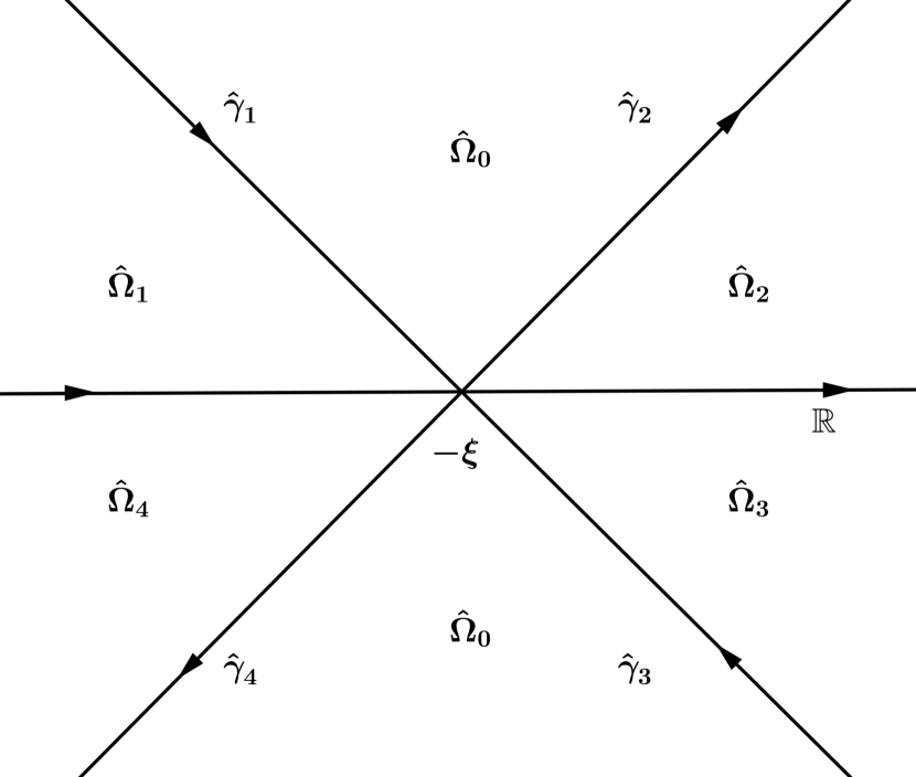
Figure 1:

$\hat{\Gamma}=\hat{\gamma}_{1}\cup...\cup\hat{\gamma}_{4}$

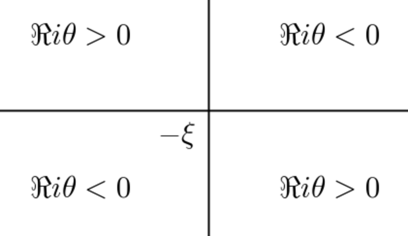
Figure 2:

Signature table

Then $\hat{M}$ satisfies the following RH problem with jumps across $\hat{\Gamma}$:

$$\begin{array}[]{lcl}\hat{M}_{+}(x,t,k)=\hat{M}_{-}(x,t,k)\hat{J}(x,t,k),\,\,k\in\hat{\Gamma},\\ \hat{M}(x,t,k)\rightarrow I,\,\,k\rightarrow\infty,\end{array}$$ (3.14)

where

$$\hat{J}(x,t,k)=\begin{cases}\begin{pmatrix}1&\frac{\sigma r_{2}(k)\delta^{2}(k,\xi)}{1+\sigma r_{1}(k)r_{2}(k)}e^{-2it\theta}\\ 0&1\\ \end{pmatrix},&k\in\hat{\gamma}_{1},\\ \begin{pmatrix}1&0\\ r_{1}(k)\delta^{-2}(k,\xi)e^{2it\theta}&1\\ \end{pmatrix},&k\in\hat{\gamma}_{2},\\ \begin{pmatrix}1&-\sigma r_{2}(k)\delta^{2}(k,\xi)e^{-2it\theta}\\ 0&1\\ \end{pmatrix},&k\in\hat{\gamma}_{3},\\ \begin{pmatrix}1&0\\ \frac{-r_{1}(k)\delta^{-2}(k,\xi)}{1+\sigma r_{1}(k)r_{2}(k)}e^{2it\theta}&1\\ \end{pmatrix},&k\in\hat{\gamma}_{4}.\end{cases}$$ (3.15)

Under assumption (3.10), $\hat{M}$ can have a singularity at $k=-\xi$ weaker than $(k+\xi)^{-1/2}$ and thus the standard arguments show that the solution of the RH problem (3.14) is unique, if exists.

The signature table for $\operatorname{Im}\theta$ clearly shows that the jump matrix $\hat{J}(x,t,k)$ for the deformed problem (3.14) converges rapidly, as $t\to\infty$ to the identity matrix for all $k\in{\hat{\Gamma}\setminus\{-\xi\}}$, and the convergence is uniform outside any fixed neighborhood of $-\xi$.

3.3 Reduction to a model RH problem

According to the general scheme of the asymptotic analysis of RH problems with a stationary phase point of $\theta$, near which the uniform decay to $I$ of the jump matrix is violated [8, 10], the solution of the original RH problem is compared with that of a problem modified in a neighborhood of this point using a rescaled spectral parameter. Since the rescaling is dictated by $\theta(k)$, and $\theta$ in our case is the same as in the case of the NLS equation, the rescaled spectral parameter $z$ is introduced in the same way, by

$$k=\frac{z}{\sqrt{8t}}-\xi.$$ (3.16)

Then

$$e^{2it\theta}=e^{i\frac{z^{2}}{2}-4it\xi^{2}}.$$

Near $k=-\xi$, the functions involved in the jump matrix (3.15) can be approximated as follows:

$$r_{j}(k(z))\approx r_{j}(-\xi),\quad j=1,2,$$

$$\delta(k(z),\xi)\approx\left(\frac{z}{\sqrt{8t}}\right)^{i\nu(-\xi)}e^{\chi(-\xi)}.$$

This suggests the following strategy (we basically follow [20]) for the asymptotic analysis, as $t\to\infty$, of the solution of the RH problem (3.14) and, consequently, $q(x,t)$:

1. introduce the local parametrix, i.e., the solution $m^{\Gamma}(\xi,z)$ of the RH problem in the $z$ plane relative to $\Gamma=\gamma_{1}\cup...\cup\gamma_{4}$ (see Figure 3):

   $$\left\{\begin{array}[]{lcl}m^{\Gamma}_{+}(\xi,z)=m^{\Gamma}_{-}(\xi,z)j^{\Gamma}(\xi,z),\,\,z\in\Gamma\\ m^{\Gamma}(\xi,z)\rightarrow I,\,\,z\rightarrow\infty,\end{array}\right.$$ (3.17)

   where

   $$j^{\Gamma}(\xi,z)=\begin{cases}\begin{pmatrix}1&\frac{\sigma r_{2}(-\xi)}{1+\sigma r_{1}(-\xi)r_{2}(-\xi)}e^{-i\frac{z^{2}}{2}}z^{2i\nu(-\xi)}\\ 0&1\\ \end{pmatrix},&k\in\gamma_{1},\\ \begin{pmatrix}1&0\\ r_{1}(-\xi)e^{i\frac{z^{2}}{2}}z^{-2i\nu(-\xi)}&1\\ \end{pmatrix},&k\in\gamma_{2},\\ \begin{pmatrix}1&-\sigma r_{2}(-\xi)e^{-i\frac{z^{2}}{2}}z^{2i\nu(-\xi)}\\ 0&1\\ \end{pmatrix},&k\in\gamma_{3},\\ \begin{pmatrix}1&0\\ \frac{-r_{1}(-\xi)}{1+\sigma r_{1}(-\xi)r_{2}(-\xi)}e^{i\frac{z^{2}}{2}}z^{-2i\nu(-\xi)}&1\\ \end{pmatrix},&k\in\gamma_{4}.\end{cases}$$ (3.18)

2. using $m^{\Gamma}(\xi,z)$, introduce $\tilde{m}_{0}(x,t,k)$ for $k$ near $-\xi$:

   $$\tilde{m}_{0}(x,t,k)=\Delta(\xi,t)m^{\Gamma}(\xi,z(k))\Delta^{-1}(\xi,t),$$ (3.19)

   where

   $$\Delta(\xi,t)=e^{(2it\xi^{2}+\chi(-\xi))\sigma_{3}}(8t)^{-\frac{i\nu(-\xi)}{2}\sigma_{3}};$$ (3.20)

3. using $\tilde{m}_{0}(x,t,k)$, introduce $\hat{m}(x,t,k)$:

   $$\hat{m}(x,t,k)=\begin{cases}\hat{M}(x,t,k)\tilde{m}_{0}^{-1}(x,t,k),&|k+\xi|<\varepsilon\\ \hat{M}(x,t,k),&\text{otherwise}\end{cases}$$ (3.21)

   (with some small $\varepsilon>0$); then $\hat{m}(x,t,k)$ is the solution of the following RH problem:

   $$\begin{cases}\hat{m}_{+}(x,t,k)=\hat{m}_{-}(x,t,k)\hat{v}(x,t,k),&k\in\hat{\Gamma}_{1}\\ \hat{m}(x,t,k)\to I,&k\to\infty\end{cases}$$ (3.22)

   where $\hat{\Gamma}_{1}=\hat{\Gamma}\cup\{k:|k+\xi|=\varepsilon\}$ (the circle $\{k:|k+\xi|=\varepsilon\}$ is counterclockwise oriented) and

   $$\hat{v}(x,t,k)=\begin{cases}\tilde{m}_{0-}(x,t,k)\hat{J}(x,t,k)\tilde{m}_{0+}^{-1}(x,t,k),&k\in\hat{\Gamma},|k+\xi|<\varepsilon\\ \tilde{m}_{0}^{-1}(x,t,k),&|k+\xi|=\varepsilon\\ \hat{J}(x,t,k),&\text{otherwise}\end{cases}$$ (3.23)

   Let us note, that (2.23) implies

   $$q(x,t)=2i\lim_{k\rightarrow\infty}k\,\hat{m}_{12}(x,t,k).$$ (3.24)

4. estimating $\hat{v}-I$, establish estimates for the large-$t$ behavior of $\hat{m}(x,t,k)$ and thus $\hat{M}(x,t,k)$ in view of establishing the large-$t$ behavior of $q(x,t)=2i(\hat{M}_{1})_{12}(x,t)$ (cf. (2.23)), where $(\hat{M}_{1})_{12}(x,t)$ comes from the large-$k$ development of $\hat{M}$: $\hat{M}(x,t,k)=I+\frac{\hat{M}_{1}(x,t)}{k}+\dots$.

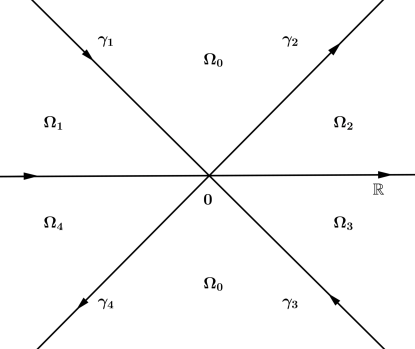
Figure 3:

$\Gamma=\gamma_{1}\cup...\cup\gamma_{4}$

Let us discuss the implementation of this strategy. Concerning item (i), we notice that $m^{\Gamma}(\xi,z)$ can be constructed as follows:

$$m^{\Gamma}(\xi,z)=m_{0}(\xi,z)D^{-1}_{j}(\xi,z),\qquad z\in\Omega_{j},\,\,j=0,\ldots,4,$$ (3.25)

where

$$D_{0}(\xi,z)=e^{-i\frac{z^{2}}{4}\sigma_{3}}z^{i\nu(-\xi)\sigma_{3}},$$

$$\begin{matrix}D_{1}(\xi,z)=D_{0}(\xi,z)\begin{pmatrix}1&\frac{\sigma r_{2}(-\xi)}{1+\sigma r_{1}(-\xi)r_{2}(-\xi)}\\ 0&1\\ \end{pmatrix},&&D_{2}(\xi,z)=D_{0}(\xi,z)\begin{pmatrix}1&0\\ r_{1}(-\xi)&1\\ \end{pmatrix},\\ D_{3}(\xi,z)=D_{0}(\xi,z)\begin{pmatrix}1&-\sigma r_{2}(-\xi)\\ 0&1\\ \end{pmatrix},&&D_{4}(\xi,z)=D_{0}(\xi,z)\begin{pmatrix}1&0\\ \frac{-r_{1}(-\xi)}{1+\sigma r_{1}(-\xi)r_{2}(-\xi)}&1\\ \end{pmatrix},\end{matrix}$$

and $m_{0}(\xi,z)$ is the solution of the following RH problem, relative to $\mathbb{R}$, with a constant jump matrix:

$$\left\{\begin{array}[]{lcl}m_{0+}(\xi,z)=m_{0-}(\xi,z)j_{0}(\xi),\,\,z\in\mathbb{R},\\ m_{0}(\xi,z)=\left(I+O(1/z)\right)e^{-i\frac{z^{2}}{4}\sigma_{3}}z^{i\nu(-\xi)\sigma_{3}},\,\,z\rightarrow\infty,\end{array}\right.$$ (3.26)

where

$$j_{0}(\xi)=\begin{pmatrix}1+\sigma r_{1}(-\xi)r_{2}(-\xi)&\sigma r_{2}(-\xi)\\ r_{1}(-\xi)&1\end{pmatrix}.$$ (3.27)

The solution $m_{0}(\xi,z)$ of this problem can be given explicitly, in terms of the parabolic cylinder functions, see Appendix A.

From (3.23) and (3.25) it follows that $\hat{w}(x,t,k):=\hat{v}(x,t,k)-I\in L^{2}(\hat{\Gamma}_{1})\cap L^{\infty}(\hat{\Gamma}_{1})$ and thus we can closely follow the proof of Theorem 2.1 in [20], particularly, in what is related to the (large-$t$) estimates for $\hat{w}(x,t,k)$. Here the major difference between our case and that in [20] is that the factor $\Delta(\xi,t)$, see (3.20) ($D(\xi,t)$ in the notations in [20]) now contains an increasing (with $t$) term $t^{\frac{\operatorname{Im}\nu(-\xi)}{2}}$ or $t^{\frac{-\operatorname{Im}\nu(-\xi)}{2}}$ (depending on the sign of $\operatorname{Im}\nu(-\xi)$). Particularly, this implies that in our case, the estimates for the columns of the $\hat{w}(x,t,k)$ (see Claims 1-4 in [20]) acquire the following form (recall that $A^{(j)}$ denotes the j-th column of a matrix $A$):

$$\hat{w}^{(j)}(\xi,t,\cdot)=O\left(t^{-\frac{1}{2}+(-1)^{j}\operatorname{Im}\nu(-\xi)}e^{-a(k+\xi)^{2}t}\ln t\right),\quad t\to\infty,\quad k\in\hat{\Gamma}\cap\{|k+\xi|<\varepsilon\},\,a>0,\,j=1,2.$$

uniformly with respect to $k$ in the given ranges. Moreover,

$$\|\hat{w}^{(j)}(\xi,t,\cdot)\|_{L^{2}(\hat{\Gamma}_{1})}=O\left(t^{-\frac{1}{2}+(-1)^{j}\operatorname{Im}\nu(-\xi)}\right),\quad t\to\infty,\,j=1,2,$$

$$\|\hat{w}(\xi,t,\cdot)\|_{L^{\infty}(\hat{\Gamma}_{1})}=O\left(t^{-\frac{1}{2}+|\operatorname{Im}\nu(-\xi)|}\ln t\right),\quad t\to\infty,$$

and

$$\|\hat{w}^{(j)}(\xi,t,\cdot)\|_{L^{1}(\hat{\Gamma})}=O\left(t^{-1+(-1)^{j}\operatorname{Im}\nu(-\xi)}\ln t\right),\quad t\to\infty,\,j=1,2.$$

Particularly, the above estimates imply

$$\|{\cal C}_{\hat{w}}\|_{{\cal B}(L^{2}(\hat{\Gamma}_{1}))}=O\left(t^{-\frac{1}{2}+|\operatorname{Im}\nu(-\xi)|}\ln t\right),\quad t\to\infty,$$ (3.28)

where the integral operator ${\cal C}_{\hat{w}}:L^{2}(\hat{\Gamma}_{1})+L^{\infty}(\hat{\Gamma}_{1})\to L^{2}(\hat{\Gamma}_{1})$ is defined by ${\cal C}_{\hat{w}}f={\cal C}_{-}(f\hat{w})$ and ${\cal C}$ is the Cauchy operator associated with $\hat{\Gamma}_{1}$:

$$({\cal C}f)(z)=\frac{1}{2\pi i}\int_{\hat{\Gamma}_{1}}\frac{f(s)}{s-z}ds,\qquad z\in{\mathbb{C}}\setminus\hat{\Gamma}_{1}.$$

Moreover,

$$\|\mu(\xi,t,\cdot)-I\|_{L^{2}(\hat{\Gamma}_{1})}=O\left(t^{-\frac{1}{2}+|\operatorname{Im}\nu(-\xi)|}\right),\mbox{ as }\,t\to\infty,$$

where $\mu=I+L^{2}(\hat{\Gamma}_{1})$ is the solution of the integral equation

$$\mu-{\cal C}_{\hat{w}}\mu=I$$ (3.29)

(or, more precisely, $\mu-I\in L^{2}(\hat{\Gamma}_{1})$ is the solution of the integral equation $(I-{\cal C}_{\hat{w}})(\mu-I)={\cal C}_{\hat{w}}I$).

Finally, we use the representation for $\hat{m}$ (where $\hat{m}(x,t,k)\equiv\hat{m}(\xi,t,k)$):

$$\hat{m}(\xi,t,k)=I+{\cal C}(\mu\hat{w})=I+\frac{1}{2\pi i}\int_{\hat{\Gamma}_{1}}\mu(\xi,t,s)\hat{w}(\xi,t,s)\frac{ds}{s-k},$$

which implies that

$$\lim\limits_{k\to\infty}k(\hat{m}(\xi,t,k)-I) =-\frac{1}{2\pi i}\int_{\hat{\Gamma}_{1}}\mu(\xi,t,k)\hat{w}(\xi,t,k)dk$$ (3.30)

$$=-\frac{1}{2\pi i}\int_{|k+\xi|=\varepsilon}\mu(\xi,t,k)(\tilde{m}_{0}^{-1}(\xi,t,k)-I)dk-\frac{1}{2\pi i}\int_{\hat{\Gamma}}\mu(\xi,t,k)\hat{w}(\xi,t,k)dk.$$

Using the estimates above and the restriction on the $\operatorname{Im}\nu(-\xi)$, namely $-\frac{1}{2}<\operatorname{Im}\nu(-\xi)<\frac{1}{2}$ (see (3.9) and (3.10)), the columns of the second term in (3.30) can be estimated, as $t\to\infty$, as follows (cf. [20]):

$$\int_{\hat{\Gamma}}\left(\mu(\xi,t,k)\hat{w}(\xi,t,k)\right)^{(1)}\,dk=\begin{cases}O\left(t^{-1}\right),&\operatorname{Im}\nu(-\xi)>0,\\ O\left(t^{-1}\ln t\right),&\operatorname{Im}\nu(-\xi)=0,\\ O\left(t^{-1+2|\operatorname{Im}\nu(-\xi)|}\right),&\operatorname{Im}\nu(-\xi)<0,\end{cases}$$ (3.31a)

and

$$\int_{\hat{\Gamma}}\left(\mu(\xi,t,k)\hat{w}(\xi,t,k)\right)^{(2)}\,dk=\begin{cases}O\left(t^{-1+2|\operatorname{Im}\nu(-\xi)|}\right),&\operatorname{Im}\nu(-\xi)>0,\\ O\left(t^{-1}\ln t\right),&\operatorname{Im}\nu(-\xi)=0,\\ O\left(t^{-1}\right),&\operatorname{Im}\nu(-\xi)<0.\end{cases}$$ (3.31b)

On the other hand, the main asymptotic terms comes from the calculations of the first term using the large-$t$ asymptotics for $\tilde{m}_{0}^{-1}(\xi,t,k)$, which, in turn, comes from the large-$z$ asymptotics for $m^{\Gamma}(\xi,z)$. Indeed, using

$$m^{\Gamma}(\xi,z)=I+\frac{i}{z}\begin{pmatrix}0&\beta(\xi)\\ -\gamma(\xi)&0\end{pmatrix}+O(z^{-2}),\quad z\to\infty$$

(where $\beta(\xi)$ and $\gamma(\xi)$ are given in (4.14) and (4.15), see Appendix A) and (3.19) with (3.20), we have

$$\tilde{m}_{0}^{-1}(\xi,t,k)=\Delta(\xi,t)(m^{\Gamma})^{-1}(\xi,\sqrt{8t}(k+\xi))\Delta^{-1}(\xi,t)=I+\frac{B(\xi,t)}{\sqrt{8t}(k+\xi)}+\tilde{r}_{1}(\xi,t),$$

where

$$B(\xi,t)=\begin{pmatrix}0&-i\beta(\xi)e^{4it\xi^{2}+2\chi(-\xi)}(8t)^{-i\nu(-\xi)}\\ i\gamma(\xi)e^{-4it\xi^{2}-2\chi(-\xi)}(8t)^{i\nu(-\xi)}&0\end{pmatrix}.$$ (3.32)

and the columns of the remainder are

$$\tilde{r}_{1}^{(j)}(\xi,t)=O\left(t^{-1+(-1)^{j}\operatorname{Im}\nu(-\xi)}\right),\quad t\to\infty,j=1,2.$$ (3.33)

Therefore, for the first $2\times 2$ matrix in the right-hand side of (3.30) we have

$$\int_{|k+\xi|=\varepsilon}\mu(\xi,t,k)\left(\tilde{m}_{0}^{-1}(\xi,t,k)-I\right)\,dk=\int_{|k+\xi|=\varepsilon}\left(\tilde{m}_{0}^{-1}(\xi,t,k)-I\right)\,dk$$ (3.34)

$$+\int_{|k+\xi|=\varepsilon}\left(\mu(\xi,t,k)-I\right)\left(\tilde{m}_{0}^{-1}(\xi,t,k)-I\right)\,dk=2\pi i\tilde{B}(\xi,t)+\tilde{r}_{1}(\xi,t)+\tilde{r}_{2}(\xi,t),$$

where (recall that $\{k:|k+\xi|=\varepsilon\}$ is oriented counterclockwise)

$$\tilde{B}(\xi,t)=\begin{pmatrix}0&-i\beta(\xi)e^{4it\xi^{2}+2\chi(-\xi)}(8t)^{-\frac{1}{2}-i\nu(-\xi)}\\ i\gamma(\xi)e^{-4it\xi^{2}-2\chi(-\xi)}(8t)^{-\frac{1}{2}+i\nu(-\xi)}&0\end{pmatrix},$$ (3.35)

and the remainder $\tilde{r}_{2}(\xi,t)\equiv\|\mu-I\|_{L^{2}(|k+\xi|=\varepsilon)}\cdot O\left(\tilde{B}(\xi,t)\right)$ can be estimated, as $t\to\infty$, as follows:

$$\tilde{r}_{2}^{(1)}(\xi,t)=\begin{cases}O\left(t^{-1}\right),&\operatorname{Im}\nu(-\xi)\geq 0,\\ O\left(t^{-1+2|\operatorname{Im}\nu(-\xi)|}\right),&\operatorname{Im}\nu(-\xi)<0,\end{cases}$$ (3.36a)

and

$$\tilde{r}_{2}^{(2)}(\xi,t)=\begin{cases}O\left(t^{-1+2|\operatorname{Im}\nu(-\xi)|}\right),&\operatorname{Im}\nu(-\xi)\geq 0,\\ O\left(t^{-1}\right),&\operatorname{Im}\nu(-\xi)<0.\end{cases}$$ (3.36b)

Finally, taking into account (3.31), (3.33), (3.34) and (3.36), equation (3.30) takes the form

$$\lim\limits_{k\to\infty}k(\hat{m}(\xi,t,k)-I)=\tilde{B}(\xi,t)+\tilde{r}_{3}(\xi,t),$$ (3.37)

where $\tilde{r}_{3}(\xi,t)\equiv\tilde{r}_{1}(\xi,t)+\tilde{r}_{2}(\xi,t)-\frac{1}{2\pi i}\int_{\hat{\Gamma}}\mu(\xi,t,k)w(\xi,t,k)\,dk$ can be estimated similarly as in (3.31), and we arrive at

Theorem 1.

Consider the Cauchy problem (1.1) with the initial data $q_{0}(x)\in L^{1}(\mathbb{R})$. Assume that the spectral functions associated with $q_{0}(x)$ via (2.11)–(2.16) are such that:

1. $a_{1}(k)$ and $a_{2}(k)$ have no zeros in $\overline{\mathbb{C}^{+}}$ and $\overline{\mathbb{C}^{-}}$ respectively;

2. $\int_{-\infty}^{a}d\arg(1+\sigma r_{1}(\zeta)r_{2}(\zeta))\in(-\pi,\pi)$ for all $a\in\mathbb{R}$, where $r_{1}(k)=\frac{b(k)}{a_{1}(k)}$, $r_{2}(k)=\frac{\overline{b(-{k})}}{a_{2}(k)}$.

Assuming that the solution $q(x,t)$ of (1.1) exists and $q(x,t)\in L^{1}(\mathbb{R})$ for all $t>0$, its long-time asymptotics is as follows:

$$q(x,t)=t^{-\frac{1}{2}+\operatorname{Im}\nu(-\xi)}p(-\xi)\exp\left\{4it\xi^{2}-i\operatorname{Re}\nu(-\xi)\ln t\right\}+R(\xi,t),\quad t\rightarrow\infty,$$ (3.38)

uniformly for $x\in\mathbb{R}$ chosen from compact subsets, where $\xi=\frac{x}{4t}$,

$$\nu(-\xi)=-\frac{1}{2\pi}\ln(1+\sigma r_{1}(-\xi)r_{2}(-\xi)),$$

$$p(-\xi)=\dfrac{\sqrt{\pi}\exp\left\{-\frac{\pi}{2}\nu(-\xi)+\frac{\pi i}{4}+2\chi(-\xi)-3i\nu(-\xi)\ln 2\right\}}{r_{1}(-\xi)\Gamma(-i\nu(-\xi))},$$

where $\Gamma(\cdot)$ is Euler’s Gamma function and

$$\chi(-\xi)=-\frac{1}{2\pi i}\int_{-\infty}^{-\xi}\ln(-\xi-\zeta)d_{\zeta}\ln(1+\sigma r_{1}(\zeta)r_{2}(\zeta)),$$

and the remainder is estimated as follows:

$$R(\xi,t)=\begin{cases}O\left(t^{-1+2|\operatorname{Im}\nu(-\xi)|}\right),&\operatorname{Im}\nu(-\xi)>0,\\ O\left(t^{-1}\ln t\right),&\operatorname{Im}\nu(-\xi)=0,\\ O\left(t^{-1}\right),&\operatorname{Im}\nu(-\xi)<0.\end{cases}$$

Remark 4.

In contrast to the local NLS equation, where the main asymptotic term decays to $0$ as $O(t^{-1/2})$ along any ray $\xi=const$, the power decay rate in the case of the NNLS depends, in general, on $\xi$, through the imaginary part of $\nu(-\xi)$.

Remark 5.

The symmetry (2.29) implies that the solution $q(x,t)$ can also be obtained by

$$q(x,t)=-2i\lim_{k\to\infty}k\overline{M_{21}(-x,t,k)}=-2i\lim_{k\to\infty}k\overline{\hat{m}_{21}(-x,t,k)},$$

It follows from (4.14) and (4.15) (taking into account (3.11), (3.12) and (2.28)) that

$$\gamma(\xi)=-\sigma e^{2(\overline{\chi(\xi)}+\chi(-\xi))}\overline{\beta(-\xi)},$$ (3.39)

and, therefore, the asymptotic formula for $q(x,t)$ can be also obtained via the (21) entry in (3.37), which is, due to (3.11) and (3.39), consistent with the asymptotic formula (3.38).

Remark 6.

In the case of even initial data, the solution of the Cauchy problem (1.1) is also even and thus it satisfies the classical (local) NLS equation. In this case, $r_{1}(k)=\bar{r}_{2}(k)=:r(k)$ and thus

$$\nu(-\xi)=-\frac{1}{2\pi}\ln(1+\sigma|r(-\xi)|^{2}),$$

$$\chi(k)=-\frac{1}{2\pi i}\int_{-\infty}^{-\xi}\ln(k-\zeta)d_{\zeta}\ln(1+\sigma|r(\zeta)|^{2}),$$

and the asymptotic formula takes the well-known form [10]

$$q(x,t)=t^{-\frac{1}{2}}p(-\xi)\exp\left\{4it\xi^{2}-i\nu(-\xi)\ln t\right\}+O(t^{-1}\ln t),\qquad t\rightarrow\infty,$$ (3.40)

where

$$|p(-\xi)|^{2}=\frac{\sigma}{4\pi}\ln(1+\sigma|r(-\xi)|^{2})$$

and

$$\arg p(-\xi)=-3\nu(-\xi)\ln 2+\frac{\pi}{4}+\arg\Gamma(i\nu)-\arg r(-\xi)-2i\chi(-\xi).$$

Remark 7.

A sufficient condition for assumptions (i) and (ii) in Theorem 1 to hold can be written in terms of $\|q_{0}(x)\|_{L^{1}(\mathbb{R})}$ :

$$\int_{-\infty}^{\infty}|q_{0}(x)|\,dx<0.817.$$ (3.41)

Indeed, by (2.11) and (2.15), $a_{1}(k)$ can be estimated, following [6], by using the Neumann series for the solution $\psi_{1}$ of the Volterra integral equation

$$\psi_{1}(x,k)=1-\sigma\int_{-\infty}^{x}\overline{q_{0}}(-y)\int_{y}^{x}e^{2ik(y-z)}q_{0}(z)\,dz\,\psi_{1}(y,k)\,dy.$$ (3.42)

Introducing $Q_{0}(x)=\int_{-\infty}^{x}|q_{0}(x)|\,dx$, $R_{0}(x)=\int_{-\infty}^{x}|q_{\,0}(-x)|\,dx$, the estimates of the Neumann series give

$$|\psi_{1}(x,k)-1|\leq Q_{0}(x)R_{0}(x)+\frac{1}{(2!)^{2}}Q_{0}^{2}(x)R_{0}^{2}(x)+\frac{1}{(3!)^{2}}Q_{0}^{3}(x)R_{0}^{3}(x)+\ldots=I_{0}(2\sqrt{Q_{0}(x)R_{0}(x)})-1,$$

where $I_{0}(\cdot)$ is the modified Bessel function. Since $R_{0}(\infty)=Q_{0}(\infty)$, it follows that if $I_{0}(2Q_{0}(\infty))<2$ (which holds true, in particular, if $Q_{0}(\infty)<0.817$), then $a_{1}(k)$ for $\operatorname{Im}k\in\overline{\mathbb{C}^{+}}$ can be represented as $a_{1}(k)=1+F_{1}(k)$ with $|F_{1}(k)|<1$. Similarly for $a_{2}(k)$ for $\operatorname{Im}k\in\overline{\mathbb{C}^{-}}$. Consequently, (i) $a_{j}(k)$, $j=1,2$ have no zeros in the respective half-planes; (ii) $\arg a_{j}(k)\in\left(-\frac{\pi}{2},\frac{\pi}{2}\right)$, which, in turn, implies item (ii) in Theorem 1 taking into account (2.26).

Remark 8.

If the Riemann–Hilbert problem (2.19)–(2.22) has a solution for all $x$ and $t$, then the standard “dressing” arguments (see, e.g., [11]) imply that the solution $q(x,t)$ of (1.1) decaying as $x\to\pm\infty$ does exist. On the other hand, if the $L^{1}$ norm of the initial data $q_{0}(x)$ is small enough, then it follows from (2.11) and (2.15) that the $L^{\infty}$ norms of $r_{1}$ and $r_{2}$ are small as well, which in turn implies (see, e.g., [9]) that the integral equation associated with the Riemann–Hilbert problem (2.19)–(2.22) (and thus the RHP itself) is solvable for all $x$ and $t$.

With this respect, we notice that the pure soliton solutions can be used (see [16]) to demonstrate that the smallness of the $H^{1}$ norm of the initial data $q_{0}(x)$ does not guarantee the global existence of the solution of (1.1).

4 Single box initial values

In Section 3 we have obtained the long-time asymptotic formula for the solution of the Cauchy problem (1.1) under assumption that the spectral functions associated with the initial data satisfy conditions (i) and (ii) in Theorem 1. In this section we verify this conditions in the case of the so-called single box initial data (cf. [4], section 11), for which the spectral functions can easily be calculated explicitly.

Consider the initial data $q_{0}(x)$ of the form

$$q_{0}(x)=\begin{cases}0,&x<0,\\ H,&0<x<L,\\ 0,&x>L,\end{cases}$$ (4.1)

where $H\in\mathbb{C}$ and $L>0$. Using equations (2.11), (2.14) and the definitions (2.15) and (2.16), the spectral functions are given by

$$a_{1}(k) =1+\frac{\sigma|H|^{2}}{4k^{2}}\left(e^{2ikL}-1\right)^{2},$$ (4.2)

$$a_{2}(k) \equiv 1,$$

$$b(k) =\frac{\sigma\,\overline{H}}{2ik}\left(1-e^{2ikL}\right).$$

Notice that since $a_{2}(k)\equiv 1$ in this case, it follows that $1+\sigma r_{1}(k)r_{2}(k)=a_{1}^{-1}(k)$ and thus $\int_{-\infty}^{\xi}d\arg(1+\sigma r_{1}(\zeta)r_{2}(\zeta))=-\int_{-\infty}^{\xi}d\arg a_{1}(\zeta)$.

Proposition 1.

Let $\sigma=1$. The following results hold:

• If $|H|L<1$, then $a_{1}(k)$ has no zeros for $k\in\overline{\mathbb{C}^{+}}$ and $\arg a_{1}(k)\in\left(-\frac{\pi}{2},\frac{\pi}{2}\right)$ for all $k\in\mathbb{R}$;

• If $|H|L>1$, then $a_{1}(k)$ has at least one zero in $\mathbb{C}^{+}$, and there exists $k\in\mathbb{R}$ such that $\int_{-\infty}^{k}d\arg a_{1}(\zeta)>\frac{\pi}{2}$.

Proof.

First, notice that $a_{1}(0)=1-|H|^{2}L^{2}\neq 0$ in both cases. Now, introducing $z=z_{1}+iz_{2}$ for $z\in\mathbb{C}^{+}$, the existence of $k\in\mathbb{C}^{+}\setminus\{0\}$ such that $a_{1}(k)=0$ is equivalent to the solvability of one of the systems

$$\left\{\begin{array}[]{lcl}e^{-z_{2}}\cos z_{1}-1=\mp\frac{z_{2}}{C}\\ e^{-z_{2}}\sin z_{1}=\pm\frac{z_{1}}{C}\end{array}\right.$$ (4.3)

where $C=|H|L$ and $z=2kL$ ($z\neq 0$). Setting $z_{1}=0$, the system (4.3) reduces to the equations $e^{-z_{2}}-1=\frac{z_{2}}{C}$ or $e^{-z_{2}}-1=-\frac{z_{2}}{C}$; the first equation has no solutions with $z_{2}>0$ whereas the second one has a solution with $z_{2}>0$ if and only if $C>1$. In the case $C<1$, the second equations in (4.3) have no solutions with $z_{1}\neq 0$ and $z_{2}\geq 0$, and thus in this case $a_{1}(k)$ has no zeros in $\overline{\mathbb{C}^{+}}$.

Concerning the argument of $a_{1}(k)$, we notice that if $|H|L<1$, then $\operatorname{Re}a_{1}(k)=1-\frac{|H|^{2}}{k^{2}}\sin^{2}kL\cos 2kL>0$ for $k\in\mathbb{R}$ and, therefore, $\arg a_{1}(k)\in\left(-\frac{\pi}{2},\frac{\pi}{2}\right)$ in this case. On the other hand, if $|H|L>1$, then there exists $\delta>0$ such that $\operatorname{Re}a_{1}(k)<0$ for all $k\in(-\delta,\delta)$ and, moreover, $\operatorname{Im}a_{1}(k)=-\frac{|H|^{2}}{k^{2}}\sin^{2}kL\sin 2kL>0$ for $k\in(-\delta,0)$ and $\operatorname{Im}a_{1}(k)<0$ for $k\in(0,\delta)$. ∎

Proposition 1 gives an example of a set of initial data such that if $\|q_{0}(x)\|_{L^{1}(\mathbb{R})}<1$ for $q_{0}$ in this set, then the both assumptions (i) and (ii) in Theorem 1 hold, and, on the other hand, if $\|q_{0}(x)\|_{L^{1}(\mathbb{R})}>1$, then the both assumptions do not hold simultaneously. The next example illustrate the situation, when assumption (i) holds, but (ii) does not.

Proposition 2.

Let $\sigma=-1$. Then there exist $\varepsilon>0$ such that for $\frac{\pi}{2}<|H|L<\frac{\pi}{2}+\varepsilon$, $a_{1}(k)$ has no zeros in $\overline{\mathbb{C}^{+}}$, but there exists $k\in\mathbb{R}$ such that $\int_{-\infty}^{k}d\arg a_{1}(\zeta)>\frac{\pi}{2}$.

Proof.

First, notice that $a_{1}(0)\neq 0$ because $|H|L>1$ in the considered case. Then, in analogy with above, the existence of $k\in\mathbb{C}^{+}\setminus\{0\}$ such that $a_{1}(k)=0$ is equivalent to

$$\left\{\begin{array}[]{lcl}e^{-z_{2}}\cos z_{1}-1=\pm\frac{z_{1}}{C}\\ e^{-z_{2}}\sin z_{1}=\pm\frac{z_{2}}{C}\end{array}\right.$$ (4.4)

where, as above, $C=|H|L$ and $z=2kL$. Now notice that if $C$ is close to $\frac{\pi}{2}$, then the system $(\ref{sb2})$ has no solutions with $z_{2}=0$ and $z_{1}\neq 0$. Further, the second equation of (4.4) implies that there are no solutions with $z_{1}=0$, and the first equation implies that if $z_{1}$ is the real part of a solution, then it must satisfy $|z_{1}|\leq 2C$.

Due to the symmetry relation $a_{1}(k)=\overline{a_{1}(-\bar{k})}$, it is sufficient to show that (4.4) has no solutions with $z_{1}>0$ and $z_{2}>0$. Let us look for the solution of (4.4) in the form $z_{2}=\rho z_{1}$ with some $\rho>0$; then (4.4) reduces to

$$\left\{\begin{array}[]{lcl}e^{-\rho z_{1}}(\rho\cos z_{1}-\sin z_{1})-\rho=0\\ e^{-\rho z_{1}}\sin z_{1}=\pm\frac{\rho z_{1}}{C}\end{array}\right.$$

which implies, in particular, the equation for $z_{1}$:

$$e^{-\rho z_{1}}(\rho\cos z_{1}-\sin z_{1})=\rho.$$

But this equation has no solutions for $0<z_{1}\leq\pi+2\varepsilon$ for $\varepsilon>0$ small enough, which implies that $a_{1}(k)$ has no zeros with $|z_{1}|\leq 2C$ with $C$ satisfying $\frac{\pi}{2}<C<\frac{\pi}{2}+\varepsilon$.

Now we notice that if $C>\frac{\pi}{2}$, then $\operatorname{Re}a_{1}(k)=1+\frac{|H|^{2}}{k^{2}}\sin^{2}kL\cos 2kL<0$ for $k\in(\frac{\pi}{2L}-\delta,\frac{\pi}{2L}+\delta)$ with some $\delta>0$. At the same time, $\operatorname{Im}a_{1}(k)\equiv\frac{|H|^{2}}{k^{2}}\sin^{2}kL\sin 2kL>0$ for $k\in(\frac{\pi}{2L}-\delta,\frac{\pi}{2L})$ and, therefore, $|\int_{-\infty}^{k}d\arg a_{1}(\zeta)|>\frac{\pi}{2}$ for such $k$. ∎

Appendix A

The model RH problem (3.26) can be solved explicitly, similarly to the case of the local NLS, in terms of the parabolic cylinder functions (see [18, 13]). Indeed, since the jump matrix $j_{0}(\xi)$ is independent of $z$, it follows that the logarithmic derivative $\frac{d}{dz}m_{0}\cdot m_{0}^{-1}$ is an entire function. Taking into account the asymptotic condition in the RH problem (3.26) and using Liouville’s theorem one concludes (cf. [20]) that $m_{0}(\xi,z)$ satisfies the following ODE

$$\frac{d}{dz}m_{0}(\xi,z)+\begin{pmatrix}\frac{iz}{2}&\beta(\xi)\\ \gamma(\xi)&\frac{-iz}{2}\\ \end{pmatrix}m_{0}(\xi,z)=0$$ (4.5)

with some $\beta(\xi)$ and $\gamma(\xi)$; moreover (recall (3.25)), $\beta(\xi)=-i(m^{\Gamma}_{1})_{12}(\xi)$, $\gamma(\xi)=i(m^{\Gamma}_{1})_{21}(\xi)$, where $m_{0}(\xi,z)=(I+\frac{m^{\Gamma}_{1}(\xi)}{z}+\ldots)e^{-i\frac{z^{2}}{4}\sigma_{3}}z^{i\nu(-\xi)\sigma_{3}}$ as $z\to\infty$.

Observe that a solution to (4.5) can be written in the form

$$m_{0}(\xi,z)=\begin{pmatrix}(m_{0})_{11}(\xi,z)&\dfrac{\left(\frac{d}{dz}-i\frac{z}{2}\right)(m_{0})_{22}(\xi,z)}{-\gamma(\xi)}\\ \dfrac{\left(\frac{d}{dz}+i\frac{z}{2}\right)(m_{0})_{11}(\xi,z)}{-\beta(\xi)}&(m_{0})_{22}(\xi,z)\end{pmatrix}$$ (4.6)

where the functions $(m_{0})_{jj}(\xi,z)$, $j=1,2$ satisfy the parabolic cylinder equations

$$\frac{d^{2}}{dz^{2}}(m_{0})_{11}(\xi,z)+\left(\frac{i}{2}-\beta(\xi)\gamma(\xi)+\frac{z^{2}}{4}\right)(m_{0})_{11}(\xi,z)=0,$$ (4.7)

$$\frac{d^{2}}{dz^{2}}(m_{0})_{22}(\xi,z)+\left(-\frac{i}{2}-\beta(\xi)\gamma(\xi)+\frac{z^{2}}{4}\right)(m_{0})_{22}(\xi,z)=0$$ (4.8)

and thus can be expressed in terms of the parabolic cylinder functions $D_{i\tilde{\nu}(-\xi)}(\pm ze^{\frac{\pi i}{4}})$ and $D_{-i\tilde{\nu}(-\xi)}(\pm ze^{\frac{{3\pi i}}{4}})$ respectively, where $\tilde{\nu}(-\xi):=\beta(\xi)\gamma(\xi)$. Indeed, using the formula for derivative of the parabolic cylinder function $D_{a}(z)$:

$$\frac{d}{dz}D_{a}(z)=\frac{z}{2}D_{a}(z)-D_{a+1}(z)$$

and comparing the asymptotic condition in (3.26) with the asymptotic formula for $D_{a}(z)$:

$$D_{a}(z)=z^{a}e^{-\frac{z^{2}}{4}}\left(1-\frac{a(a-1)}{2z^{2}}+O(z^{-4})\right),\,\,\arg z\in\left(-\tfrac{3\pi}{4};\tfrac{3\pi}{4}\right),\quad z\to\infty,\quad a\in\mathbb{C},$$

one obtains

$$(m_{0})_{11}(\xi,z)=\begin{cases}e^{-\frac{3\pi}{4}\tilde{\nu}(-\xi)}D_{i\tilde{\nu}(-\xi)}\left(e^{-\frac{3\pi i}{4}}z\right),&\operatorname{Im}z>0,\\ e^{\frac{\pi}{4}\tilde{\nu}(-\xi)}D_{i\tilde{\nu}(-\xi)}\left(e^{\frac{\pi i}{4}}z\right),&\operatorname{Im}z<0,\end{cases}$$ (4.9)

$$(m_{0})_{22}(\xi,z)=\begin{cases}e^{\frac{\pi}{4}\tilde{\nu}(-\xi)}D_{-i\tilde{\nu}(-\xi)}\left(e^{-\frac{\pi i}{4}}z\right),&\operatorname{Im}z>0,\\ e^{-\frac{3\pi}{4}\tilde{\nu}(-\xi)}D_{-i\tilde{\nu}(-\xi)}\left(e^{\frac{3\pi i}{4}}z\right),&\operatorname{Im}z<0.\end{cases}$$ (4.10)

Now, calculating $m_{0-}^{-1}(\xi,z)m_{0+}(\xi,z)$ for $z\in\mathbb{R}$ from (4.6), (4.9) and (4.10), noting that $m_{0-}^{-1}(\xi,z)m_{0+}(\xi,z)=m_{0-}^{-1}(\xi,0)m_{0+}(\xi,0)$, and using the equalities

$$\begin{matrix}D_{a}(0)=\dfrac{2^{\frac{a}{2}}\sqrt{\pi}}{\Gamma\left(\frac{1-a}{2}\right)},&&D_{a}^{{}^{\prime}}(0)=-\dfrac{2^{\frac{1+a}{2}}\sqrt{\pi}}{\Gamma\left(-\frac{a}{2}\right)},\\ \\ \Gamma\left(\frac{1}{2}-i\frac{a}{2}\right)\Gamma\left(\frac{1}{2}+i\frac{a}{2}\right)=\dfrac{\pi}{\cosh\frac{\pi a}{2}},\,a\neq 2i\mathbb{Z}+1,&&\Gamma\left(-i\frac{a}{2}\right)\Gamma\left(i\frac{a}{2}\right)=\dfrac{2\pi}{a\sinh\frac{\pi a}{2}},\,a\neq 2i\mathbb{Z},\end{matrix}$$ (4.11)

where $\Gamma(\cdot)$ is Euler’s Gamma function, we find that

$$m_{0-}^{-1}(\xi,z)m_{0+}(\xi,z)\equiv m_{0-}^{-1}(\xi,0)m_{0+}(\xi,0)=\begin{pmatrix}\frac{e^{\frac{\pi\tilde{\nu}}{4}}2^{\frac{i\tilde{\nu}}{2}}\sqrt{\pi}}{\Gamma\left(\frac{1-i\tilde{\nu}}{2}\right)}&\frac{e^{\frac{3\pi}{4}(i-\tilde{\nu})}2^{\frac{1-i\tilde{\nu}}{2}}\sqrt{\pi}}{\gamma(\xi)\Gamma\left(\frac{i\tilde{\nu}}{2}\right)}\\ \frac{e^{\frac{\pi}{4}(i+\tilde{\nu})}2^{\frac{1+i\tilde{\nu}}{2}}\sqrt{\pi}}{\beta(\xi)\Gamma\left(\frac{-i\tilde{\nu}}{2}\right)}&\frac{e^{-\frac{3\pi\tilde{\nu}}{4}}2^{-\frac{i\tilde{\nu}}{2}}\sqrt{\pi}}{\Gamma\left(\frac{1+i\tilde{\nu}}{2}\right)}\end{pmatrix}^{-1}$$

$$\times\begin{pmatrix}\frac{e^{-\frac{3\pi\tilde{\nu}}{4}}2^{\frac{i\tilde{\nu}}{2}}\sqrt{\pi}}{\Gamma\left(\frac{1-i\tilde{\nu}}{2}\right)}&\frac{e^{\frac{\pi}{4}(\tilde{\nu}-i)}2^{\frac{1-i\tilde{\nu}}{2}}\sqrt{\pi}}{\gamma(\xi)\Gamma\left(\frac{i\tilde{\nu}}{2}\right)}\\ \frac{e^{-\frac{3\pi}{4}(i+\tilde{\nu})}2^{\frac{1+i\tilde{\nu}}{2}}\sqrt{\pi}}{\beta(\xi)\Gamma\left(\frac{-i\tilde{\nu}}{2}\right)}&\frac{e^{\frac{\pi\tilde{\nu}}{4}}2^{\frac{-i\tilde{\nu}}{2}}\sqrt{\pi}}{\Gamma\left(\frac{1+i\tilde{\nu}}{2}\right)}\end{pmatrix}=\begin{pmatrix}e^{-2\pi\tilde{\nu}}&\frac{e^{-\frac{\pi\tilde{\nu}}{2}}e^{-\frac{\pi i}{4}}\sqrt{2\pi}}{\gamma(\xi)\Gamma(i\tilde{\nu})}\\ \frac{e^{-\frac{\pi\tilde{\nu}}{2}}e^{-\frac{3\pi i}{4}}\sqrt{2\pi}}{\beta(\xi)\Gamma(-i\tilde{\nu})}&1\end{pmatrix}$$ (4.12)

where $\tilde{\nu}\equiv\tilde{\nu}(-\xi)$. Consequently, equating this to $j_{0}(\xi)$ defined in (3.27):

$$\begin{pmatrix}e^{-2\pi\tilde{\nu}}&\frac{e^{-\frac{\pi\tilde{\nu}}{2}}e^{-\frac{\pi i}{4}}\sqrt{2\pi}}{\gamma(\xi)\Gamma(i\tilde{\nu})}\\ \frac{e^{-\frac{\pi\tilde{\nu}}{2}}e^{-\frac{3\pi i}{4}}\sqrt{2\pi}}{\beta(\xi)\Gamma(-i\tilde{\nu})}&1\end{pmatrix}=\begin{pmatrix}1+\sigma r_{1}(-\xi)r_{2}(-\xi)&\sigma r_{2}(-\xi)\\ r_{1}(-\xi)&1\end{pmatrix}$$ (4.13)

we obtain that $\tilde{\nu}(\xi)\equiv\nu(\xi)$, where $\nu(\xi)$ is defined in (3.9), and that $\beta(\xi)$ and $\gamma(\xi)$ are expressed in terms of $r_{1}(\xi)$ and $r_{2}(\xi)$ (“inverse monodromy problem”, cf. [13]) as follows:

$$\beta(\xi)=\dfrac{\sqrt{2\pi}e^{-\frac{\pi}{2}\nu(-\xi)}e^{-\frac{3\pi i}{4}}}{r_{1}(-\xi)\Gamma(-i\nu(-\xi))},$$ (4.14)

$$\gamma(\xi)=\dfrac{\sigma\sqrt{2\pi}e^{-\frac{\pi}{2}\nu(-\xi)}e^{-\frac{\pi i}{4}}}{r_{2}(-\xi)\Gamma(i\nu(-\xi))}.$$ (4.15)

References

- [1] M. J. Ablowitz, B.-F. Feng, X.-D. Luo and Z. H. Musslimani, Inverse scattering transform for the nonlocal reverse space-time sine-Gordon, sinh-Gordon and nonlinear Schrödinger equations with nonzero boundary conditions, preprint arXiv:1703.02226.
- [2] M. J. Ablowitz, X.-D. Luo and Z. H. Musslimani, Inverse scattering transform for the nonlocal nonlinear Schrödinger equation with nonzero boundary conditions, preprint arXiv:1612.02726.
- [3] M. J. Ablowitz and Z. H. Musslimani, Integrable nonlocal nonlinear Schrödinger equation, Phys. Rev. Lett. 110 064105 (2013).
- [4] M. J. Ablowitz and Z. H. Musslimani, Inverse scattering transform for the integrable nonlocal nonlinear Schrödinger equation, Nonlinearity 29 (2016), 915–946.
- [5] M. J. Ablowitz and Z. H. Musslimani, Integrable nonlocal nonlinear equations, Stud. Appl. Math. 139 (2017), 7–59.
- [6] M. J. Ablowitz and H. Segur, Solitons and Inverse Scattering Transform. SIAM Studies in Applied Mathematics 4. Philadelphia, PA: Society for Industrial and Applied Mathematics (SIAM), 1981.
- [7] C. M. Bender and S. Boettcher, Real spectra in non-Hermitian Hamiltonians having P-T symmetry, Phys. Rev. Lett. 80 (1998), 5243.
- [8] P. A. Deift and X. Zhou, A steepest descend method for oscillatory Riemann–Hilbert prob- lems. Asymptotics for the MKdV equation, Ann. Math. 137, no. 2 (1993): 295–368.
- [9] P. A. Deift and X. Zhou, Long-time asymptotics for solutions of the NLS equation with initial data in a weighted Sobolev space, Comm. Pure Appl. Math. 56 (2003), 1029–1077.
- [10] P. A. Deift, A. R. Its and X. Zhou, Long-time asymptotics for integrable nonlinear wave equations. In Important developments in Soliton Theory 1980-1990, edited by A. S. Fokas and V. E. Zakharov, New York: Springer, 181–204, 1993.
- [11] L. D. Faddeev and L. A. Takhtajan, Hamiltonian Methods in the Theory of Solitons. Springer Series in Soviet Mathematics. Springer-Verlag, Berlin, 1987.
- [12] A. S. Fokas, Integrable multidimensional versions of the nonlocal nonlinear Schrödinger equation, Nonlinearity 29 (2016), 319–324.
- [13] A. S. Fokas, A.R. Its, A.A. Kapaev and V. Yu. Novokshenov, Painleve Transcendents. The Riemann–Hilbert Approach, AMS, 2006.
- [14] V. V. Konotop, J. Yang and D. A. Zezyulin, Nonlinear waves in PT-symmetric systems, Rev. Mod. Phys. 88, 035002 (2016).
- [15] T. Gadzhimuradov and A. Agalarov, Towards a gauge-equivalent magnetic structure of the nonlocal nonlinear Schrödinger equation, Phys. Rev. A, 93, 062124 (2016).
- [16] F. Genoud, Instability of an integrable nonlocal NLS, C. R. Math. Acad. Sci. Paris 355 (2017), 299–303. arXiv:1612.03139.
- [17] V. S. Gerdjikov and A. Saxena, Complete integrability of nonlocal nonlinear Schrödinger equation, J. Math. Phys. 58, 013502 (2017).
- [18] A. R. Its, Asymptotic behavior of the solutions to the nonlinear Schrödinger equation, and isomonodromic deformations of systems of linear differential equations, Doklady Akad. Nauk SSSR 261, no. 1 (1981), 14–18.
- [19] J. Lenells, Matrix Riemann-Hilbert problems with jumps across Carleson contours, preprint arXiv:1401.2506.
- [20] J. Lenells, The nonlinear steepest descent method for Riemann-Hilbert problems of low regularity, Indiana Univ. Math. 66 (2017), 1287–1332.
- [21] M. Li and T. Xu, Dark and antidark soliton interactions in the nonlocal nonlinear Schrödinger equation with the self-induced parity-time-symmetric potential, Phys. Rev. E 91, 033202 (2015).
- [22] L. Ma and Z. Zhu, Nonlocal nonlinear Schrödinger equation and its discrete version: Soliton solutions and gauge equivalence, J. Math. Phys. 57, 083507 (2016).
- [23] A.K. Sarma, M.-A. Miri, Z.H. Musslimani and D.N. Christodoulides, Continuous and discrete Schrödinger systems with parity-time-symmetric nonlinearities, Phys. Rev. E 89, 052918 (2014).
- [24] T. Valchev, On a nonlocal nonlinear Schrödinger equation. In Slavova, A.(ed) Mathematics in Industry, Cambridge Scholars Publishing pp. 36–52 (2014).
- [25] V. E. Zakharov and S. V. Manakov, Asymptotic behavior of nonlinear wave systems integrated by the inverse method. Zh. Eksp. Teor. Fiz. 71 (1976), 203–215 (in Russian); Sov. Phys. JETP, 44, no. 1 (1976), 106–112 (in English).