CLOT Norm Minimization for Continuous Hands-off Control

Abstract

In this paper, we consider hands-off control via minimization of the CLOT (Combined $L$-One and Two) norm. The maximum hands-off control is the $L^{0}$-optimal (or the sparsest) control among all feasible controls that are bounded by a specified value and transfer the state from a given initial state to the origin within a fixed time duration. In general, the maximum hands-off control is a bang-off-bang control taking values of $\pm 1$ and $0$. For many real applications, such discontinuity in the control is not desirable. To obtain a continuous but still relatively sparse control, we propose to use the CLOT norm, a convex combination of $L^{1}$ and $L^{2}$ norms. We show by numerical simulations that the CLOT control is continuous and much sparser (i.e. has longer time duration on which the control takes 0) than the conventional EN (elastic net) control, which is a convex combination of $L^{1}$ and squared $L^{2}$ norms. We also prove that the CLOT control is continuous in the sense that, if $O(h)$ denotes the sampling period, then the difference between successive values of the CLOT-optimal control is $O(\sqrt{h})$, which is a form of continuity. Also, the CLOT formulation is extended to encompass constraints on the state variable.

Keywords: Optimal control, convex optimization, sparsity, maximum hands-off control, bang-off-bang control

1 Introduction

Sparsity has recently emerged as an important topic in signal/image processing, machine learning, statistics, etc. If $y\in{\mathbb{R}}^{m}$ and $A\in{\mathbb{R}}^{m\times n}$ are specified with $m<n$, then the equation $y=Ax$ is underdetermined and has infinitely many solutions for $x$ if $A$ has rank $m$. Finding the sparsest solution (that is, the solution with the fewest number of nonzero elements) can be formulated as

$$\min_{z}\|z\|_{0}\mathrm{~{}~{}subject~{}to~{}~{}}Az=b.$$

However, this problem is NP hard, as shown in [1]. Therefore other approaches have been proposed for this purpose. This area of research is known as “sparse regression.” One of the most popular is LASSO [2], also referred to as forgetting [3], or basis pursuit [4], in which the $\ell^{0}$-norm is replaced by the $\ell^{1}$-norm. Thus the problem becomes

$$\min_{z}\|z\|_{1}\mathrm{~{}~{}subject~{}to~{}~{}}Az=b.$$

The advantage of LASSO is that it is a convex optimization problem and therefore very large problems can be solved efficiently, for example by using the Matlab-based package cvx [5]. Moreover, under mild technical assumptions, the LASSO-optimal solution has no more than $m$ nonzero components [6]. However, the exact location of the nonzero components is very sensitive to the vector $y$. To overcome this deficiency, another approach known as the Elastic Net was proposed in [7], where the $\ell^{1}$ norm in LASSO is replaced by a weighted sum of $\ell^{1}$ and squared $\ell^{2}$ norms. This leads to the optimization problem

$$\min_{z}\lambda_{1}\|z\|_{1}+\lambda_{2}\|z\|_{2}^{2}\mathrm{~{}~{}subject~{}to~{}~{}}Az=b,$$

where $\lambda_{1}$ and $\lambda_{2}$ are positive weights such that $\lambda_{1}+\lambda_{2}=1$. It is shown in [7, Theorem 1] that the EN formulation gives the grouping effect; If two columns of the matrix $A$ are highly correlated, then the corresponding components of the solution for $x$ have nearly equal values. This ensures that the solution for $x$ is not overly sensitive to small changes in $y$. The name “elastic net” is meant to suggest a stretchable fishing net that retains all the big fish.

During the past decade and a half, another research area known as “compressed sensing” has witnessed a great deal of interest. In compressed sensing, the matrix $A$ is not specified; rather, the user gets to choose the integer $m$ (known as the number of measurements), as well as the matrix $A$. The objective is to choose the matrix $A$ as well as a corresponding “decooder” map $\Delta:{\mathbb{R}}^{m}\rightarrow{\mathbb{R}}^{n}$ such that, the unknown vector $x$ is sparse and the measurement vector $y$ equals $Ax$, then $\Delta(Ax)=x$ for all sufficiently sparse vectors $x$. More generally, if measurement vector $y=Ax+\eta$ where $\eta$ is the measurement noise, and the vector $x$ is nearly sparse (but not exactly sparse), then the recovered vector $\Delta(Ax+\eta)$ should be sufficiently close to the true but unknown vector $x$. This is referred to as “robust sparse recovery.” Minimizing the $\ell_{1}$-norm is among the more popular decoders. See the books by [8], [9], and [10] for the theory and some applications. Due to its similarity to the LASSO formulation of [2], this approach to compressed sensing is also referred to as LASSO.

Until recently the situation was that LASSO achieves robust sparse recovery in compressed sensing, but did not achieve the grouping effect in sparse regression. On the flip side, EN achieves the grouping effect, but it was not known whether it achieves robust sparse recovery. A recent paper [11] sheds some light on this problem. It is shown in [11] that EN does not achieve robust sparse recovery. To achieve both the grouping effect in sparse regression as well as robust sparse recovery in compressed sensing, [11] has proposed the CLOT (Combined $L$-One and Two) formulation:

$$\min_{z}\lambda_{1}\|z\|_{1}+\lambda_{2}\|z\|_{2}\mathrm{~{}~{}subject~{}to~{}~{}}Az=b,$$

where $\lambda_{1}>0$, $\lambda_{2}>0$, and $\lambda_{1}+\lambda_{2}=1$. The difference between EN and CLOT is the $\ell^{2}$ norm term; EN has the squared $\ell^{2}$ norm while CLOT has the pure $\ell^{2}$ norm. This slight change leads to both the grouping effect and robust sparse recovery, as shown in [11].

In parallel with these advances in sparse regression and recovery of unknown sparse vectors, sparsity techniques have also been applied to control. Sparsity-promoting optimization has been applied to networked control in [12], where quantization errors and data rate can be reduced at the same time by sparse representation of control packets. Other examples of control applications include optimal controller placement by [13, 14, 15], design of feedback gains by [16, 17], state estimation by [18], to name a few.

More recently, a novel control called the maximum hands-off control has been proposed in [19] for continuous-time systems. The maximum hands-off control is the $L^{0}$-optimal control (the control that has the minimum support length) among all feasible controls that are bounded by a fixed value and transfer the state from a given initial state to the origin within a fixed time duration. Such a control is effective for reduction of electricity or fuel consumption; an electric/hybrid vehicle shuts off the internal combustion engine (i.e. hands-off control) when the vehicle is stopped or the speed is lower than a preset threshold; see [20] for example. Railway vehicles also utilize hands-off control, often called coasting control, to cut electricity consumption; see [21] for details. In [19], the authors have proved the theoretical relation between the maximum hands-off control and the $L^{1}$ optimal control under the assumption of normality. Also, important properties of the maximum hands-off control have been proved in [22] for the convexity of the value function, and in [23] for necessary conditions of optimality, and in [24] for the discreteness.

In general, the maximum hands-off control is a bang-off-bang control taking values of $\pm 1$ and $0$. For many real applications, such a discontinuity property is not desirable. To obtain a continuous but still sparse control, [19] has proposed to use a combined $L^{1}$ and squared $L^{2}$ minimization, like EN mentioned above. Let us call this control an EN control. As in the case of EN in the vector optimization, the EN control often shows much less sparse (i.e. has a larger $L^{0}$ norm) than the maximum hands-off control. Then, in [25], we have proposed to use the CLOT norm, a convex combination of $L^{1}$ and non-squared $L^{2}$ norms. The minimum CLOT-norm control is called the CLOT control. In [25], we have shown by numerical simulation that the CLOT control is continuous and much sparser (i.e. has longer time duration on which the control takes 0) than the conventional EN control.

In [19], both the LASSO and EN approaches to hands-off control are solved in continuous-time. It is shown, using Pontryagin’s minimum principle, that the LASSO solution is bang-off-bang, while the EN solution is continuous. However, the CLOT formulation cannot be addressed via Pontryagin’s principle. Therefore it is not clear whether the resulting optimal control is continuous. In the present paper, we study the discretized problem, and show that as the sampling interval $h$ approaches zero, the difference between successive control signals is $O(\sqrt{h})$, which is a form of continuity. We extend this result to the case where, in addition to constraints on the control signal, there are also constraints on the state $x(t)$.

The remainder of this article is organized as follows. In Section 2, we formulate the control problem considered in this paper. In Section 3, we give a discretization method to numerically compute the optimal control. In Section 4, we give the additional state constraints for the optimization problems. The limiting behaviour of the CLOT optimal control is stated in Section 5. Results of the numerical computations on a variety of problems without any state constriants are presented in Section 6. Results of the numerical computations on a variety of problems with state constriants are presented in Section 6. These examples illustrate the advantages of the CLOT control compared with the maximum hands-off control and the EN control. We present some conclusions in Section 8.

Notation

Let $T>0$ and $m\in\mathbb{N}$. For a continuous-time signal $u(t)\in\mathbb{R}$ over a time interval $[0,T]$, we define its $L^{p}$ ($p\geq 1$) and $L^{\infty}$ norms respectively by

$$\|u\|_{p}\triangleq\bigg{\{}\int_{0}^{T}|u(t)|^{p}dt\bigg{\}}^{1/p},~{}\|u\|_{\infty}\triangleq\sup_{t\in[0,T]}|u(t)|.$$

We denote the set of all signals with $\|u\|_{p}<\infty$ by $L^{p}[0,\,T]$ for $p\geq 1$ or $p=\infty$. We define the $L^{0}$ norm of a signal $u(t)$ on the interval $[0,T]$ as

$$\|u\|_{0}\triangleq\int_{0}^{T}\phi_{0}(u(t))dt,$$

where $\phi_{0}$ is the $L^{0}$ kernel function defined by

$$\phi_{0}(\alpha)\triangleq\begin{cases}1,&\text{~{}if~{}}\alpha\neq 0,\\ 0,&\text{~{}if~{}}\alpha=0\end{cases}$$ (1)

for a scalar $\alpha\in\mathbb{R}$. The $L^{0}$ norm can be represented by

$$\|u\|_{0}=\mu_{\mathrm{L}}\bigl{(}\mathrm{supp}(u)\bigr{)},$$

where $\mathrm{supp}(u)$ is the support of the signal $u$, and $\mu_{\mathrm{L}}$ is the Lebesgue measure on ${\mathbb{R}}$.

2 Problem Formulation

Let us consider a linear time-invariant system described by

$$\frac{dx}{dt}(t)=Ax(t)+Bu(t),~{}t\geq 0,~{}x(0)=\xi.$$ (2)

Here we assume that $x(t)\in{\mathbb{R}}^{n}$, $u(t)\in{\mathbb{R}}$, and the initial state $x(0)=\xi$ is fixed and given. The control objective is to drive the state $x(t)$ from $x(0)=\xi$ to the origin at time $T>0$, that is

$$x(T)=0.$$ (3)

We limit the control $u(t)$ to satisfy

$$\|u\|_{\infty}\leq U_{\max}$$ (4)

for fixed $U_{\max}>0$.

If the system (2) is controllable and the final time $T$ is larger than the optimal time $T^{\ast}$ (the minimal time in which there exist a control $u(t)$ that drives $x(t)$ from $x(0)=\xi$ to the origin; see [26]), then there exists at least one $u(t)\in L^{\infty}[0,T]$ that satisfies equations (2), (3), and (4). Let us call such a control a feasible control. From (2) and (3), any feasible control $u(t)$ on $[0,T]$ satisfies

$$0=x(T)=e^{AT}\xi+\int_{0}^{T}e^{A(T-t)}Bu(t)dt,$$

or

$$\int_{0}^{T}e^{-At}Bu(t)dt+\xi=0.$$ (5)

Define a linear operator $\Phi:L^{\infty}[0,T]\rightarrow{\mathbb{R}}^{n}$ by

$$\Phi u\triangleq\int_{0}^{T}e^{-At}Bu(t)dt,\quad u\in L^{\infty}[0,T].$$

By this, we define the set ${\mathcal{U}}$ of the feasible controls by

$$\mathcal{U}\triangleq\left\{u\in L^{\infty}:\Phi u+\xi=0,~{}\|u\|_{\infty}\leq 1\right\}.$$ (6)

The problem of the maximum hands-off control is then described by

$$\underset{u}{\mathrm{minimize}}~{}~{}\|u\|_{0}\mathrm{~{}~{}subject~{}to~{}~{}}u\in\mathcal{U}.$$ (7)

The $L^{0}$ problem (7) is very hard to solve since the $L^{0}$ cost function is non-convex and discontinuous. For this problem, [19] has shown that the $L^{0}$ optimal control in (7) is equivalent to the following $L^{1}$ optimal control:

$$\underset{u}{\mathrm{minimize}}~{}~{}\|u\|_{1}\mathrm{~{}~{}subject~{}to~{}~{}}u\in\mathcal{U},$$ (8)

if the plant is normal, that is, if the system (2) is controllable and the matrix $A$ is nonsingular. Let us call the $L^{1}$ optimal control as the LASSO control. If the plant is normal, then the LASSO control is in general a bang-off-bang control that is piecewise constant taking values in $\{0,\pm 1\}$. The discontinuity of the LASSO solution is not desirable in real applications, and a smoothed solution is also proposed in [19] as

$$\underset{u}{\mathrm{minimize}}~{}~{}\|u\|_{1}+\lambda\|u\|_{2}^{2}\mathrm{~{}~{}subject~{}to~{}~{}}u\in\mathcal{U},$$ (9)

where $\lambda>0$ is a design parameter for smoothness. Let us call this control the EN (elastic net) control. In [19], it is proved that the solution of (9) is a continuous function on $[0,T]$.

While the EN control is continuous, it is shown by numerical experiments that the EN control is not sometimes sparse. This is an analogy of the EN for finite-dimensional vectors that EN does not achieve robust sparse recovery. Borrowing the idea of CLOT in [11], we define the CLOT optimal control problem by

$$\underset{u}{\mathrm{minimize}}~{}~{}\|u\|_{1}+\lambda\|u\|_{2}\mathrm{~{}~{}subject~{}to~{}~{}}u\in\mathcal{U}.$$ (10)

We call this optimal control the CLOT control.

3 Discretization

Since the problems (8)–(10) are infinite dimensional, we should approximate it to finite dimensional problems. For this, we adopt the time discretization.

First, we divide the time interval $[0,T]$ into $N$ subintervals, $[0,T]=[0,h)\cup\dots\cup[(N-1)h,Nh]$, where $h$ is the discretization step (or the sampling period) such that $T=Nh$. We assume that the state $x(t)$ and the control $u(t)$ in (2) are constant over each subinterval. On the discretization grid, $t=0,h,\dots,Nh$, the continuous-time system (2) is described as

$$\hat{x}_{k+1}=A_{d}\hat{x}_{k}+B_{d}\hat{u}_{k},\quad k=0,1,\dots,N-1,$$ (11)

where $\hat{x}_{k}\triangleq x(kh)$, $\hat{u}_{k}\triangleq u(kh)$, and

$$A_{d}\triangleq e^{Ah},\quad B_{d}\triangleq\int_{0}^{h}e^{At}Bdt.$$ (12)

Define the control vector

$$\hat{u}\triangleq[\hat{u}_{0},\hat{u}_{1},\dots,\hat{u}_{N-1}]^{\top}.$$ (13)

Note that the final state $x(T)$ can be described as

$$x(T)=\hat{x}_{N}=A_{d}^{N}\xi+\Phi_{N}\hat{u},$$ (14)

where

$$\Phi_{N}\triangleq\begin{bmatrix}A_{d}^{N-1}B_{d},&A_{d}^{N-2}B_{d},&\dots,&B_{d}\end{bmatrix}.$$ (15)

Then the set $\mathcal{U}$ in (6) is approximately represented by

$${\mathcal{U}}_{N}\triangleq\left\{\hat{u}\in{\mathbb{R}}^{N}:A_{d}^{N}\xi+\Phi_{N}\hat{u}=0,~{}\|\hat{u}\|_{\infty}\leq 1\right\}.$$ (16)

Next, we approximate the $L^{1}$ norm of $u$ by

$$\begin{split}\|u\|_{1}&=\int_{0}^{T}|u(t)|dt\\ &=\sum_{k=0}^{N-1}\int_{kh}^{(k+1)h}|u(t)|dt\\ &\approx\sum_{k=0}^{N-1}\int_{kh}^{(k+1)h}|\hat{u}_{k}|dt\\ &=\sum_{k=0}^{N-1}|\hat{u}_{k}|h\\ &=\|\hat{u}\|_{1}h.\end{split}$$ (17)

In the same way, we obtain approximation of the $L^{2}$ norm of $u$ as

$$\|u\|_{2}^{2}=\int_{0}^{T}|u(t)|^{2}dt\approx\|\hat{u}\|_{2}^{2}h.$$ (18)

Finally, the optimal control problems (8), (9) and (10) can be approximated by

$$\underset{\hat{u}\in{\mathbb{R}}^{N}}{\mathrm{minimize}}~{}~{}h\|\hat{u}\|_{1}\mathrm{~{}~{}subject~{}to~{}~{}}\hat{u}\in{\mathcal{U}}_{N},$$ (19)

$$\underset{\hat{u}\in{\mathbb{R}}^{N}}{\mathrm{minimize}}~{}~{}h\|\hat{u}\|_{1}+h\lambda\|\hat{u}\|_{2}^{2}\mathrm{~{}~{}subject~{}to~{}~{}}\hat{u}\in{\mathcal{U}}_{N},$$ (20)

$$\underset{\hat{u}\in{\mathbb{R}}^{N}}{\mathrm{minimize}}~{}~{}h\|\hat{u}\|_{1}+\sqrt{h}\lambda\|\hat{u}\|_{2}\mathrm{~{}~{}subject~{}to~{}~{}}\hat{u}\in{\mathcal{U}}_{N}.$$ (21)

The optimization problems are convex and can be efficiently solved by numerical software packages such as cvx with Matlab; see [5] for details.

4 Optimal control with additional state contraints

In this section, additional constraints are introducted to optimization problems (19), (20) and (21) on the states to ensure that $\ell_{2}$ norm of the state at any given instant does not blow up.

The constraint is the $\ell_{2}$ norm of the state vector at any given time should not exceed a specified threshold $\theta$, that is,

$$\|\hat{x}_{k}\|_{2}\leq\theta,\qquad k\in\{1,2,\ldots,N-1\},$$ (22)

where $\hat{x}_{k}$ is the discrete-time state at time instant $k$ as defined in (11). Using (11), the states are described as

$$\begin{bmatrix}\hat{x}_{1}\\ \hat{x}_{2}\\ \hat{x}_{3}\\ \vdots\\ \hat{x}_{N-1}\end{bmatrix}=\begin{bmatrix}A_{d}\\ A_{d}^{2}\\ A_{d}^{3}\\ \vdots\\ A_{d}^{N-1}\end{bmatrix}\xi+\Psi_{N}\begin{bmatrix}\hat{u}_{0}\\ \hat{u}_{1}\\ \hat{u}_{2}\\ \vdots\\ \hat{u}_{N-2}\end{bmatrix}$$ (23)

where

$$\Psi_{N}=\begin{bmatrix}B_{d}&0&0&\dots&\dots&0\\ A_{d}B_{d}&B_{d}&0&\dots&\dots&0\\ A_{d}^{2}B_{d}&A_{d}B_{d}&B_{d}&\dots&\dots&0\\ \dots\\ \dots\\ A_{d}^{N-2}B_{d}&A_{d}^{N-3}B_{d}&A_{d}^{N-4}B_{d}&\dots&\dots&B_{d}\end{bmatrix}$$ (24)

and $\Psi_{N}\in\mathbb{R}^{(N-1)n\times(N-1)}$.

4.1 How to choose $\theta$?

The following steps are followed in order to choose $\theta$:

1. First, we solve the control optimization problems without state constraint and then we note the maximum of $\ell_{2}$ norm of the state vector, say $l_{\max}$.

2. It is to be noted that if $\theta\geq l_{\max}$, the problem is still unconstrained with respect to state. Thus, maximum value of the threshold ($\theta_{\max}$) is $l_{\max}$.

3. Then, we set $\theta$ to $\theta_{\max}$ and keep decreasing the value of $\theta$ until the optimization problems become infeasible. This gives us lower bound on $\theta$.

4. Since, the state constraints are dependent on the system, we get a range of $\theta$ that is specific to each problem.

Therefore, the optimization problems respectively become

$$\underset{\hat{u}\in{\mathbb{R}}^{N}}{\mathrm{minimize}} h\|u\|_{1}$$ (25)

$$\mathrm{subject~{}to} \hat{u}\in{\mathcal{U}}_{N},~{}~{}\|\hat{x}_{k}\|_{2}\leq\theta$$

$$k\in\{1,\cdots,N-1\}$$

for LASSO control,

$$\underset{\hat{u}\in{\mathbb{R}}^{N}}{\mathrm{minimize}} h\|\hat{u}\|_{1}+h\lambda\|\hat{u}\|_{2}^{2}$$ (26)

$$\mathrm{subject~{}to} \hat{u}\in{\mathcal{U}}_{N},~{}~{}\|\hat{x}_{k}\|_{2}\leq\theta$$

$$k\in\{1,\cdots,N-1\}$$

for EN control, and

$$\underset{\hat{u}\in{\mathbb{R}}^{N}}{\mathrm{minimize}} h\|\hat{u}\|_{1}+\sqrt{h}\lambda\|\hat{u}\|_{2}$$ (27)

$$\mathrm{subject~{}to} \hat{u}\in{\mathcal{U}}_{N},~{}~{}\|\hat{x}_{k}\|_{2}\leq\theta$$

$$k\in\{1,\cdots,N-1\}$$

for CLOT control.

5 Limiting behavior of CLOT solution

In this section, we show the limiting behaviour of CLOT optimal control.

Theorem 5.1

If $\hat{u}$ is the solution of the problem (27), then $|\hat{u}_{k}-\hat{u}_{k+1}|$ is of $O(\sqrt{h})$, where $\hat{u}_{k}$ is the $k$-th entry of $\hat{u}$.

Due to the length of the proof, it is added to the appendix B. It can be noted that the slope of $\hat{u}$ is of $O({1}/\sqrt{h})$, thus as $h\rightarrow 0$, the slope blows up, thus the CLOT optimal control closely approximates $L^{1}$ optimal control. Therefore, CLOT optimal control solution is continuous approximation of $L^{1}$ optimal control.

Corollary 5.1.1

If $\hat{u}$ is the solution of the problem (27) without state constraints (i.e. $\theta$ is sufficiently large), then $|\hat{u}_{k}-\hat{u}_{k+1}|$ is of $O(\sqrt{h})$.

6 Numerical Examples without state constraints

In this section we present numerical results from applying the CLOT norm minimization approach to seven different plants, and compare the results with those from applying LASSO and EN.

6.1 Details of Various Plants Studied

For the reader’s convenience, the details of the various plants are given in Table 1. The figure numbers show where the corresponding computational results can be found. Some conventions are adopted to reduce the clutter in the table, as described next. All plants are of the form

$$P(s)=\frac{n(s)}{d(s)},n(s)=\prod_{i=1}^{n_{z}}(s-z_{i}),d(s)=\prod_{i=1}^{n_{p}}(s-p_{i}).$$

To save space in the table, the plant zeros are not shown; $P_{3}(s)$ has a zero at $s=-2$, $P_{6}(s)$ has a zero at $s=2$, while $P_{7}(s)$ has zeros at $s=1,2$. The remaining plants do not have any zeros, so that the plant numerator equals one.

Once the plant zeros and poles are specified, the plant numerator and denominator polynomials $n,d$ were computed using the Matlab command poly. Then the transfer function was computed as P = tf(n,d), and the state space realization was computed as [A,B,C,D] = ssdata(P). The maximum control amplitude is taken $1$, so that the control must satisfy $|u(t)|\leq 1$ for $t\in[0,T]$. To save space, we use the notation ${\bf e}_{l}$ to denote an $l$-column vector whose elements all equal one. Note that in all but one case, the initial condition equals ${\bf e}_{n}$ where $n$ is the order of the plant.

Note that, with $T=20$, the problems with plants $P_{6}(s)$ and $P_{7}(s)$ are not feasible (meaning that $T$ is smaller than the minimum time needed to reach the origin); this is why we took $T=40$.

All optimization problems were solved after discretizing the interval $[0,T]$ into both 2,000 as well as 4,000 samples, to examine whether the sampling time affects the sparsity density of the computed optimal control.

No​	Plant​	Poles​	$T$​	$x(0)$​	$\lambda$​	Figs​
1	$P_{1}(s)$	0,0,0,0	20	${\bf e}_{4}$	1	1, 2
2	$P_{1}(s)$	0,0,0,0	20	${\bf e}_{4}$	0.1	3, 4
3	$P_{2}(s)$	$-0.025\pm j$	20	${\bf e}_{2}$	0.1	5, 6
4	$P_{2}(s)$	$-0.025\pm j$	20	$(10,1)^{\top}$	0.1	7, 8
5	$P_{3}(s)$	$-1\pm 0.2j$	20	${\bf e}_{4}$	0.1	9, 10
		$\pm j$
6	$P_{4}(s)$	$-5\pm j$	20	${\bf e}_{6}$	0.1	11, 12
		$-0.3\pm 2j$
		$-1\pm 2\sqrt{2}j$
7	$P_{5}(s)$	$0,0,0,0$	40	${\bf e}_{6}$	0.1	13, 14
		$\pm j$
8	$P_{6}(s)$	$0,0,0,0$	40	${\bf e}_{6}$	0.1	15, 16
		$\pm j$

Table 1: Details of various plants studied

6.2 Plots of Optimal State and Control Trajectories

The plots of the $\ell^{2}$-norm (or Euclidean norm) of the state vector trajectory and the control signal for all these examples are shown in the next several plots.

We begin with the plant $P_{1}(s)$, the fourth-order integrator. Figures 1 and 2 show the state and control trajectories when $\lambda=1$. The same system is analyzed using a smaller value of $\lambda=0.1$. One would expect that the resulting control signals would be more sparse with a smaller $\lambda$, and this is indeed the case. The results are shown in Figures 3 and 4. Based on the observation that the control signal becomes more sparse with $\lambda=0.1$ than with $\lambda=1$, all the other plants are analyzed with $\lambda=0.1$.

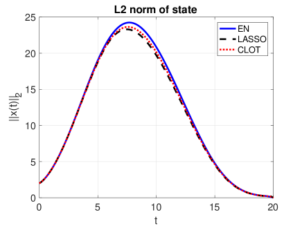
Figure 1: State trajectory for the plant $P_{1}(s)$ with the initial state $(1,1,1,1)^{\top}$ and $\lambda=1$.

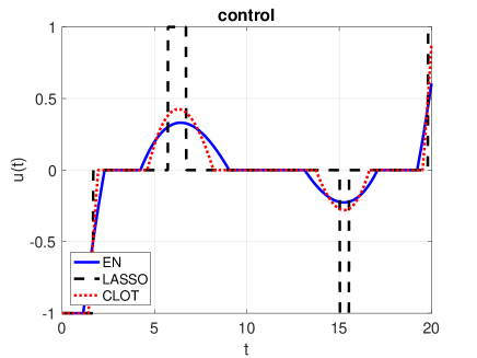
Figure 2: Control trajectory for the plant $P_{1}(s)$ with the initial state $(1,1,1,1)^{\top}$ and $\lambda=1$.

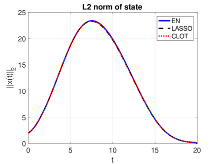
Figure 3: State trajectory for the plant $P_{1}(s)$ with the initial state $(1,1,1,1)^{\top}$ and $\lambda=0.1$.

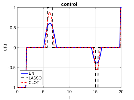
Figure 4: Control trajectory for the plant $P_{1}(s)$ with the initial state $(1,1,1,1)^{\top}$ and $\lambda=0.1$.

Figures 5 and 6 display the state trajectory and the control trajectories of the plant $P_{2}(s)$ (damped harmonic oscillator) when the initial state is $(1,1)^{\top}$. Figures 7 and 8 show the state and control trajectories with the initial state $(10,1)^{\top}$. It can be seen that, with this intial state, the control signal changes sign more frequently.

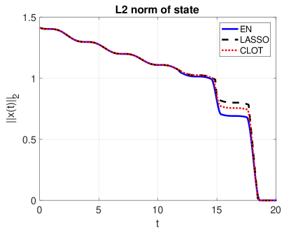
Figure 5: State trajectory for the the plant $P_{2}(s)$ with the initial state $(1,1)^{\top}$ and $\lambda=0.1$.

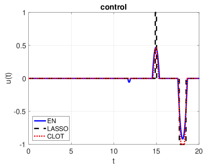
Figure 6: Control trajectory for the the plant $P_{2}(s)$ with the initial state $(1,1)^{\top}$ and $\lambda=0.1$.

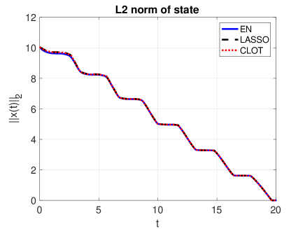
Figure 7: State trajectory for the plant $P_{2}(s)$ with the initial state $(10,1)^{\top}$ and $\lambda=0.1$.

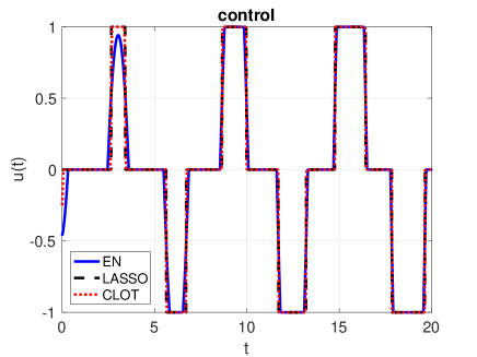
Figure 8: Control trajectory for the plant $P_{2}(s)$ with the initial state $(10,1)^{\top}$ and $\lambda=0.1$.

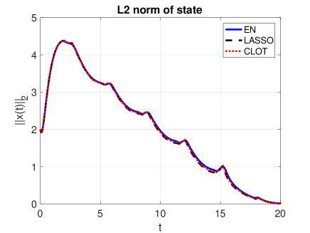
Figure 9: State trajectory for the plant $P_{3}(s)$ with the initial state $(1,1,1,1)^{\top}$ and $\lambda=0.1$.

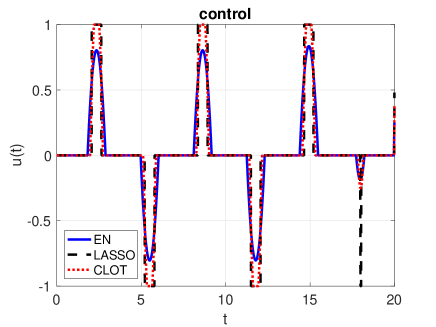
Figure 10: Control trajectory for the plant $P_{3}(s)$ with the initial state $(1,1,1,1)^{\top}$ and $\lambda=0.1$.

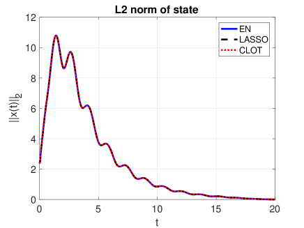
Figure 11: State trajectory for the plant $P_{4}(s)$ with the initial state $(1,1,1,1,1,1)^{\top}$ and $\lambda=0.1$.

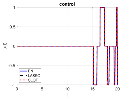
Figure 12: Control trajectory for the plant $P_{4}(s)$ with the initial state $(1,1,1,1,1,1)^{\top}$ and $\lambda=0.1$.

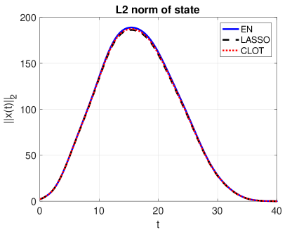
Figure 13: State trajectory for the plant $P_{5}(s)$ with the initial state $(1,1,1,1,1,1)^{\top}$ and $\lambda=0.1$.

Figure 14: Control trajectory for the plant $P_{5}(s)$ with the initial state $(1,1,1,1,1,1)^{\top}$ and $\lambda=0.1$.

Figure 15: State trajectory for the plant $P_{6}(s)$ with the initial state $(1,1,1,1,1,1)^{\top}$ and $\lambda=0.1$.

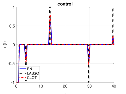
Figure 16: Control trajectory for the plant $P_{6}(s)$ with the initial state $(1,1,1,1,1,1)^{\top}$ and $\lambda=0.1$.

To compare the sparsity densities of the three control signals, we compute the fraction of time that each signal is nonzero. In this connection, it should be noted that the LASSO control signal is the solution of a linear programming problem; consequently its components exactly equal zero at many time instants. In contrast, the EN and CLOT control signals are the solutions of convex optimization problems. Consequently, there are many time instants when the control signal is “small” without being smaller than the machine zero. Therefore, to compute the sparsity density, we applied a threshold of $10^{-4}$, and treated a component of a control signal as being zero if its magnitude is smaller than this threshold. With this convention, the sparsity densities of the various control signals are as shown in Table 2. From this table it can be seen that the control signal generated using CLOT norm minimization has significantly lower sparsity density compared to that of EN, and is not much higher than that of LASSO. Also, as expected, the sparsity density of LASSO does not change with $\lambda$, whereas the sparsity densities of both EN and CLOT decrease as $\lambda$ is decreased. For this reason, in other examples we present only the results for $\lambda=0.1$.

$\lambda$	LASSO	EN	CLOT
$\lambda=1$	0.1725	0.6050	0.5900
$\lambda=0.1$	0.1725	0.3795	0.2665

Table 2: Sparsity indices of the control signals from various algorithms for the plant $P_{1}(s)$ (fourth-order integrator) with the initial state $(1,1,1,1)$.

6.3 Comparison of Sparsity Densities

In this subsection we analyze the sparsity densities, that is, the fraction of samples that are nonzero, using the three methods LASSO, EN, and CLOT. The advantage of using the sparsity density instead of the sparsity count (the absolute number of nonzero entries) is that when the sample time is reduced, the sparsity count would increase, whereas we would expect the sparsity density to remain the same. As explained above, we have applied a threshold of $10^{-4}$ in computing the sparsity densities of various control signals.

Table 3 shows the sparsity densities for the nine examples studied in Table 1, in the same order. From this table it can be seen that the CLOT norm-based control signal is always more sparse than the EN-based control signal. Indeed, in some cases the sparsity density of the CLOT control is comparable to that of the LASSO control.

No.	LASSO	EN	CLOT
1	0.1690	0.5915	0.4450
2	0.1690	0.3250	0.2535
3	0.0480	0.1130	0.0830
4	0.4055	0.5560	0.4225
5	0.1460	0.2935	0.2075
6	0.1125	0.1310	0.1175
7	0.0568	0.1490	0.1125
8	0.0568	0.1490	0.1125

Table 3: Sparsity densities for optimal controllers produced by various methods

We also increased the number of samples from 2,000 to 4,000, and the optimal values changed only in the third significant figure in almost all examples for all three methods. Therefore the figures in Table 3 are essentially equal to the Lebesgue measure of the support set divided by $T$.

7 Numerical Examples with state constraints

In this section we present numerical results from applying the CLOT norm minimization approach to two different plants imposed with state constraints on a range of thresholds ($\theta$), and compare the results with those from applying LASSO and EN.

7.1 Details of the plants

The plants $P_{1}(s)$ and $P_{7}(s)$ defined in the table 1 are used to demonstrated the results with state constraints. The parameters for each plant used for the optimization problems are listed in the table 4.

Plant	$T$	$x(0)$	$\lambda$	Range of $\theta$
$P_{1}(s)$	20	$[1,0,1,1]^{\top}$	1	(6, 10)
$P_{7}(s)$	40	$[1,0,1,1,1,1]^{\top}$	0.1	(30, 200)

Table 4: Details of various plants studied under state constraints

7.2 Comparison of Sparsity Densities

In this subsection we analyze the sparsity densities, using the three methods LASSO, EN, and CLOT across the range of $\theta$ mentioned in the table 4.

Figure 17 shows the sparsity densities of the plant $P_{1}(s)$ w.r.t. the threshold $\theta$, where the threshold is increased in steps of 0.5.Figure 18 shows the sparsity densities of the plant $P_{7}(s)$ w.r.t. the threshold $\theta$, where the threshold is increased in steps of 1. Figure 19 shows the trajectory of $\ell_{2}$ norm of the state and figure 20 shows the control trajectory of the plant $P_{1}(s)$ at intial state $[1,0,1,1]^{\top}$ with $\theta=11$.

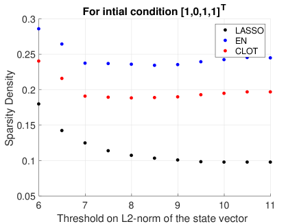
Figure 17: State threshold vs Sparsity Density for plant $P_{1}(s)$ with intial condition $[1,0,1,1]^{\top}$

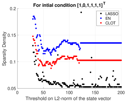
Figure 18: State threshold vs Sparsity Density for plant $P_{7}(s)$ with intial condition $[1,0,1,1,1,1]^{\top}$

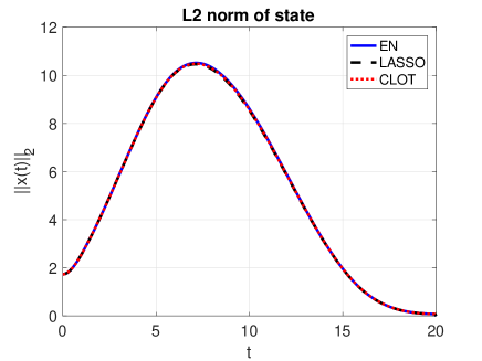
Figure 19: State trajectory for the plant $P_{1}(s)$ with the initial state $(1,0,1,1)^{\top}$ and $\theta=11$.

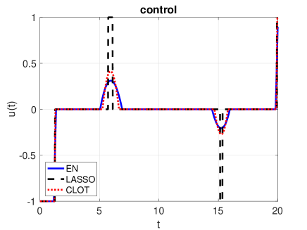
Figure 20: Control trajectory for the plant $P_{1}(s)$ with the initial state $(1,0,1,1)^{\top}$ and $\theta=11$.

There are few points in figure 18 such as $\theta$ = 123, 143 etc. where Lasso fails to converge when done by cvx package but not EN and CLOT. So, at these points Lasso has higher values for sparsity density. And, for values of $\theta$ around 130 ($\theta_{max}$) onwards, the sparsity density does not change because at these points, the control input is same.

From figures 17 and 18, it is clearly noted that CLOT control input is more sparse than than that of EN and less sparse compared to that of LASSO.

8 Conclusions

In this article, we propose the CLOT norm-based control that minimizes the weighted sum of $L^{1}$ and $L^{2}$ norms among feasible controls, to obtain a continuous control signal that is sparser than the EN control introduced in [19]. We have shown a discretization method, by which the CLOT optimal control problem can be solved via finite-dimensional convex optimization. We have shown that the CLOT control solution is continuous and it approximates $L^{1}$ optimal control solution. We have also introduced the state constraints to obtain the optimal control, to ensure the states does not blow up in order to get the optimal control. Numerical experiments have shown the advantage of the CLOT control compared with the LASSO and EN controls.

Appendix A Preliminaries

A.1 Subdifferential of norms [27]

Let $f:{\mathbb{R}}^{n}\rightarrow{\mathbb{R}}\cup\{\infty\}$ where $\mathrm{dom}(f)=\{x\in{\mathbb{R}}^{n}:f(x)<\infty\}$. A vector $g\in{\mathbb{R}}^{n}$ is a subgradient of $f$ at some $x\in\mathrm{dom}(f)$ if

$$f(z)\geq f(x)+g^{\top}(z-x),\quad\forall z\in\mathrm{dom}(f).$$ (28)

If $x\in\mathrm{Int}(\mathrm{dom}(f))$, then subgradient of $f$ at $x$, i.e., $\partial f(x)$ exists.

If a function $f$ is convex and differentiable at $x$, then its gradient at $x$ is a subgradient. A function $f$ is called subdifferentiable at $x$ if there exists at least one subgradient at $x$. The set of subgradients of $f$ at the point $x$ is called the subdifferential of $f$ at $x$, and is denoted $\partial f(x)$. A function $f$ is called subdifferentiable if it is subdifferentiable at all $x\in\mathrm{dom}(f)$.

The subdifferential $\partial f(x)$ is always a closed convex set, even if $f$ is not convex. This follows from the fact that it is the intersection of an infinite set of half-spaces:

$$\partial f(x)=\bigcap_{z\in\mathrm{dom}(f)}\{g|f(z)\geq f(x)+g^{\top}(z-x)\}.$$

A point $x^{\star}$ is a minimizer of a convex function $f$ if and only if $f$ is subdifferentiable at $x^{\star}$ and

$$0\in\partial f(x^{\star}),$$

that is, $g=0$ is a subgradient of $f$ at $x^{\star}$. This follows directly from the fact that $f(x)\geq f(x^{\star})$ for all $x\in\mathrm{dom}(f)$.

A.1.1 Vector norms and their subdifferentials

The following are the vector norms on $x\in{\mathbb{R}}^{n}$ and the corresponding subdifferentials calculated using the equation (28):

• $\ell_{1}$ norm: Let $f(x)=\|x\|_{1}$, then

  $$[\partial f(x)]_{k}=\begin{cases}\mbox{sign}(x_{k}),&\mathrm{if~{}}x_{k}\neq 0\\ y_{k},\text{ where }y_{k}\in[-1,1],&\mathrm{if~{}}x_{k}=0\end{cases}$$ (29)

• $\ell_{2}$ norm: Let $f(x)=\|x\|_{2}$, then

  $$\partial f(x)=\begin{cases}\frac{x}{\|x\|_{2}},&\mathrm{if~{}}x\neq 0\\ y,\text{ where }\|y\|_{2}\leq 1,&\mathrm{if~{}}x=0\end{cases}$$ (30)

• $\ell_{\infty}$ norm: Let $f(x)=\|x\|_{\infty}$, then

  $$[\partial f(x)]_{k}=\begin{cases}\mbox{sign}(x_{k}),&\mathrm{if~{}}x_{k}=f(x)\\ 0,&\mathrm{else}\end{cases}$$ (31)

where $k=1,2,\ldots,n$.

A.2 Karush-Kuhn-Tucker conditions

The Karush-Kuhn-Tucker (KKT) conditions are first-order necessary conditions for a solution to a convex programming to be optimal. Let us consider a convex optimization problem

$$\underset{x}{\text{minimize}} f(x)$$

subject to $$g_{i}(x)\leq 0,\quad i=1,2,\cdots,m$$

$$h_{j}(x)=0,\quad j=1,2,\cdots,l$$

where $g_{i}(x)$ are $m$ inequality constraints and $h_{j}(x)$, are $l$ equality constraints.

Let $x^{\star}$ is the optimal solution and suppose $f(x)$, $g_{i}(x)$ and $h_{j}(x)$, for all $i$ and $j$, be subdifferentiable at $x^{\star}$.

The Lagrangian formulation of the problem is given by

$$\mathcal{L}(x^{\star},\beta,\mu)=f(x)+\sum_{i=1}^{m}\mu_{i}g_{i}(x)+\sum_{j=1}^{l}\beta_{j}h_{j}(x)$$

where $\beta$ and $\mu$ are vectors of multipliers.

The KKT conditions are given as follows:
Stationarity

$$0\in\partial\mathcal{L}(x^{\star},\beta,\mu)$$

Primal Feasibility

$$g_{i}(x^{\star}) \leq 0,\quad\text{for }i=1,2,\cdots,m$$

$$h_{j}(x^{\star}) =0,\quad\text{for }j=1,2,\cdots,l$$

Dual Feasibility

$$\mu_{i}\geq 0,\quad\text{for }i=1,2,\cdots,m$$

Complementary slackness

$$\mu_{i}g_{i}(x^{\star})=0,\quad\text{for }i=1,2,\cdots,m$$

If the inequality constraints are not active, that is, $g_{i}(x^{\star})<0$ for some $i$, then the problem is unconstrained with respect to that constraint, that is, the corresponding multiplier is zero, or $\mu_{i}=0$.

Appendix B Proof of limiting behavior of CLOT solution

First, let us define the optimization problem (27) in Lagrangian form with $\beta$, $\gamma$ and $\alpha_{i}$ for all $i=1,\cdots,N-1$ as the Lagrangian parameters:

$$L(\hat{u},\lambda)\triangleq h\|\hat{u}\|_{1}+\lambda\sqrt{h}\|\hat{u}\|_{2}\\ +\beta\|A_{d}^{N}\xi+\Phi_{N}\hat{u}\|_{2}+\gamma(\|\hat{u}\|_{\infty}-1)\\ +\sum_{i=1}^{N-1}\alpha_{i}(\|A_{d}^{i}\xi+\Psi_{N}^{i}\hat{u}\|_{2}-\theta),$$ (32)

where $\hat{u}$ is the feasible optimal solution and $\Psi_{N}^{i}$ is the $i^{th}$ block row of the matrix $\Psi_{N}$, that is,

$$\Psi_{N}^{i}\triangleq\begin{bmatrix}A_{d}^{i-1}B_{d}&A_{d}^{i-2}B_{d}&\ldots,&B_{d}&0&\ldots&0\end{bmatrix}$$ (33)

The KKT conditions for this problem are given by

$$0\in\partial f(\hat{u})+\beta\partial g(\hat{u})+\gamma\partial p(\hat{u})+\sum_{i=1}^{N-1}\alpha_{i}\partial q_{i}(\hat{u}),$$ (34)

and

$$\|A_{d}^{N}\xi+\Phi_{N}\hat{u}\|_{2} =0$$ (35)

$$\|\hat{u}\|_{\infty} \leq 1$$ (36)

$$\gamma(\|\hat{u}\|_{\infty}-1) =0$$ (37)

$$\gamma \geq 0$$ (38)

$$\alpha_{i}(\|A_{d}^{i}\xi+\Psi_{N}^{i}\hat{u}\|_{2}-\theta) =0$$ (39)

$$\alpha_{i} \geq 0$$ (40)

where $f(\hat{u})=h\|\hat{u}\|_{1}+\lambda\sqrt{h}\|\hat{u}\|_{2}$, $g(\hat{u})=\|A_{d}^{N}\xi+\Phi_{N}\hat{u}\|_{2}$, $p(\hat{u})=\|\hat{u}\|_{\infty}$ and $q_{i}(\hat{u})=\|A_{d}^{i}\xi+\Psi_{N}^{i}\hat{u}\|_{2}=\|\hat{x}_{i}\|_{2}$.

Let us consider two components of $\hat{u}$, namely $k$ and $l$, assuming both are not zeros simultaneously. Let us define $a_{k}:=A_{d}^{N-k}B_{d}$, and $[\Psi_{N}^{i}]_{k}$ as the $k$-th component of $\Psi_{N}^{i}$. Expanding the partial derivatives leads to

$$\beta a_{k}^{\top}v_{k}+h\cdot\mbox{sign}(\hat{u}_{k})+\lambda\cdot\sqrt{h}\frac{\hat{u}_{k}}{\|\hat{u}\|_{2}}\\ +\gamma\cdot\mbox{sign}(\hat{u}_{k})\cdot\delta(|\hat{u}_{k}|=\|\hat{u}\|_{\infty})\\ +\sum_{i=1}^{N-1}\alpha_{i}[\Psi_{N}^{i}]_{k}^{\top}\frac{\hat{x}_{i}}{\|\hat{x}_{i}\|_{2}}=0$$ (41)

and

$$\beta a_{l}^{\top}v_{l}+h\cdot\mbox{sign}(\hat{u}_{l})+\lambda\sqrt{h}\frac{\hat{u}_{l}}{\|\hat{u}\|_{2}}\\ +\gamma\cdot\mbox{sign}(\hat{u}_{l})\cdot\delta(|\hat{u}_{l}|=\|\hat{u}\|_{\infty})\\ +\sum_{i=1}^{N-1}\alpha_{i}[\Psi_{N}^{i}]_{l}^{\top}\frac{\hat{x}_{i}}{\|\hat{x}_{i}\|_{2}}=0$$ (42)

where $v_{k}$ and $v_{l}$ are in subdifferential of $\partial\|.\|_{2}(A_{d}^{N}\xi+\Phi_{N}\hat{u})$, that is, since $A_{d}^{N}\xi+\Phi_{N}\hat{u}=0$, the subgradient is from the set of $\{v:\|v\|_{2}\leq 1\}$.

From KKT conditions (37) and (38), it can be stated that if $\|\hat{u}\|_{\infty}<1$, then $\gamma=0$ and if $\|\hat{u}\|_{\infty}=1$, then $\gamma\geq 0$.

From KKT conditions (39) and (40), it can be stated that if $\|A_{d}^{i}\xi+\Psi_{N}^{i}\hat{u}\|_{2}<\theta$, then $\alpha_{i}=0$ and if $\|A_{d}^{i}\xi+\Psi_{N}^{i}\hat{u}\|_{2}=\theta$, then $\alpha_{i}\geq 0$.

Let $l=k+1$. Then we have

• If $\hat{u}_{k}\neq 0$ and $\hat{u}_{l}\neq 0$, then $\mbox{sign}(\hat{u}_{l})=\mbox{sign}(\hat{u}_{k})$.

• If $\hat{u}_{k}=0\neq\hat{u}_{l}$, then $\mbox{sign}(\hat{u}_{k})=0$

• If $\hat{u}_{l}=0\neq\hat{u}_{k}$, then $\mbox{sign}(\hat{u}_{l})=0$

And also, $a_{k}=A_{d}a_{l}=(I+M)a_{l}$, where

$$M=e^{Ah}-I=\sum_{i=1}^{\infty}\frac{(Ah)^{i}}{i!}.$$ (43)

If $k\leq i$, then $[\Psi_{N}^{i}]_{k}=A_{d}^{i-k}B_{d}$ and if $k>i$, then $[\Psi_{N}^{i}]_{k}=0\in\mathbb{R}^{n}$.

Subtracting equations (41) and (42), when $\mbox{sign}(\hat{u}_{k})=\mbox{sign}(\hat{u}_{l})$, we have

$$\beta(a_{k}^{\top}v_{k}-a_{l}^{\top}v_{l})+\lambda\sqrt{h}\frac{(\hat{u}_{k}-\hat{u}_{l})}{\|\hat{u}\|_{2}}\\ +\gamma\bigl{\{}\mbox{sign}(u_{k})\cdot\delta(|\hat{u}_{k}|=\|\hat{u}\|_{\infty})-\mbox{sign}(u_{l})\cdot\delta(|\hat{u}_{l}|=\|\hat{u}\|_{\infty})\bigr{\}}\\ +\sum_{i=1}^{N-1}\alpha_{i}([\Psi_{N}^{i}]_{k}-[\Psi_{N}^{i}]_{l})^{\top}\frac{\hat{x}_{i}}{\|\hat{x}_{i}\|_{2}}=0$$ (44)

where

$$[\Psi_{N}^{i}]_{k}-[\Psi_{N}^{i}]_{k+1}=\begin{cases}(A_{d}-I)[\Psi_{N}^{i}]_{k+1},&\text{ if~{} }k\leq i-1,\\ B_{d},&\text{ if~{} }k=i,\\ 0,&\text{ if~{} }k>i.\\ \end{cases}$$ (45)

Equation (44) when $\mbox{sign}(\hat{u}_{k})\neq\mbox{sign}(\hat{u}_{l})$, i.e., $\hat{u}_{l}=0\neq\hat{u}_{k}$ becomes

$$\beta(a_{k}^{\top}v_{k}-a_{l}^{\top}v_{l})+h\cdot\mbox{sign}(\hat{u}_{k})+\lambda\sqrt{h}\frac{\hat{u}_{k}}{\|\hat{u}\|_{2}}\\ +\gamma\cdot\mbox{sign}(u_{k})\cdot\delta(|\hat{u}_{k}|=\|\hat{u}\|_{\infty})\\ +\sum_{i=1}^{N-1}\alpha_{i}([\Psi_{N}^{i}]_{k}-[\Psi_{N}^{i}]_{l})^{\top}\frac{\hat{x}_{i}}{\|\hat{x}_{i}\|_{2}}=0$$ (46)

The other case is similar to this one.

We also need to consider the following cases with respect to $\alpha_{i}$:

1. $\|\hat{x}_{i}\|_{2}<\theta$, $\alpha_{i}=0$.

2. $\|\hat{x}_{i}\|_{2}=\theta$, $\alpha_{i}>0$.

We need to consider the following cases for (44) with respect to $\gamma$:

1. $\|\hat{u}\|_{\infty}=1$, $|\hat{u}_{k}|<1$ and $|\hat{u}_{l}|<1$. In this case, the terms with $\gamma$ both become zero.

2. $\|\hat{u}\|_{\infty}=1$, $|\hat{u}_{k}|=1$ and $|\hat{u}_{l}|=1$. In this case, the terms with $\gamma$ will become $\mbox{sign}(\hat{u}_{k})-\mbox{sign}(\hat{u}_{l})$ and since $\mbox{sign}(\hat{u}_{k})=\mbox{sign}(\hat{u}_{l})$, the term $\gamma(\mbox{sign}(\hat{u}_{k})-\mbox{sign}(\hat{u}_{l}))$ vanishes.

3. $\|\hat{u}\|_{\infty}=1$; $|\hat{u}_{k}|=1$ and $|\hat{u}_{l}|<1$, or $|\hat{u}_{k}|<1$ and $|\hat{u}_{l}|=1$. In this case, only one term of $\gamma$ remains, and the other goes to zero. Thus, it is either $\mbox{sign}(\hat{u}_{k})$ or $\mbox{sign}(\hat{u}_{l})$ respectively.

Thus, in cases 1 and 2, the equation (44) becomes

$$\beta(a_{k}^{\top}v_{k}-a_{l}^{\top}v_{l})+\lambda\sqrt{h}\frac{(\hat{u}_{k}-\hat{u}_{l})}{\|\hat{u}\|_{2}}\\ +\sum_{i=1}^{N-1}\alpha_{i}([\Psi_{N}^{i}]_{k}-[\Psi_{N}^{i}]_{l})^{\top}\frac{\hat{x}_{i}}{\theta}=0$$ (47)

for $i$ which satisfy the case ‘b’, that is $\|\hat{x}_{i}\|_{2}=\theta$. But in case 3, the equation (44) becomes either of the following:

$$\beta(a_{k}^{\top}v_{k}-a_{l}^{\top}v_{l})+\lambda\sqrt{h}\frac{(\hat{u}_{k}-\hat{u}_{l})}{\|\hat{u}\|_{2}}+\gamma\cdot\mbox{sign}(\hat{u}_{k})\\ +\sum_{i=1}^{N-1}\alpha_{i}([\Psi_{N}^{i}]_{k}-[\Psi_{N}^{i}]_{l})^{\top}\frac{\hat{x}_{i}}{\theta}=0$$ (48)

or

$$\beta(a_{k}^{\top}v_{k}-a_{l}^{\top}v_{l})+\lambda\sqrt{h}\frac{(\hat{u}_{k}-\hat{u}_{l})}{\|\hat{u}\|_{2}}-\gamma\cdot\mbox{sign}(\hat{u}_{l})\\ +\sum_{i=1}^{N-1}\alpha_{i}([\Psi_{N}^{i}]_{k}-[\Psi_{N}^{i}]_{l})^{\top}\frac{\hat{x}_{i}}{\theta}=0$$ (49)

for $i$ which satisfy the case ‘b’, that is $\|\hat{x}_{i}\|_{2}=\theta$. We need to consider the following cases for (46) -

1. $\|\hat{u}\|_{\infty}=1$ and $|\hat{u}_{k}|<1$. In this case, the term of $\gamma(\mbox{sign}(\hat{u}_{k})-\mbox{sign}(\hat{u}_{l}))$ vanishes. Therefore, this case is similar to case 1 for (44).
   

2. $\|\hat{u}\|_{\infty}=1$ and $|\hat{u}_{k}|=1$. In this case, the term of $\gamma$ becomes $\gamma\mbox{sign}(\hat{u}_{k})$. Therefore, this case is similar to case 3 for (44).

Thus, in case 1, the equation (46) becomes

$$\beta(a_{k}^{\top}v_{k}-a_{l}^{\top}v_{l})+h\cdot\mbox{sign}(\hat{u}_{k})+\lambda\sqrt{h}\frac{\hat{u}_{k}}{\|\hat{u}\|_{2}}\\ +\sum_{i=1}^{N-1}\alpha_{i}([\Psi_{N}^{i}]_{k}-[\Psi_{N}^{i}]_{l})^{\top}\frac{\hat{x}_{i}}{\theta}=0$$ (50)

for $i$ which satisfy the case ‘b’, that is $\|\hat{x}_{i}\|_{2}=\theta$. In case 2, the equation (46) becomes

$$\beta(a_{k}^{\top}v_{k}-a_{l}^{\top}v_{l})+(h+\gamma)\cdot\mbox{sign}(\hat{u}_{k})+\lambda\sqrt{h}\frac{\mbox{sign}(\hat{u}_{k})}{\|\hat{u}\|_{2}}\\ +\sum_{i=1}^{N-1}\alpha_{i}([\Psi_{N}^{i}]_{k}-[\Psi_{N}^{i}]_{l})^{\top}\frac{\hat{x}_{i}}{\theta}=0$$ (51)

for $i$ which satisfy the case ‘b’, that is $\|\hat{x}_{i}\|_{2}=\theta$. On observation, we can say that (48), (49), (50) and (51) are similar.

Let us move further with case 3 with equation (48) (the other cases can be derived from this case):

$$\lambda\sqrt{h}\frac{(\hat{u}_{k}-\hat{u}_{l})}{\|\hat{u}\|_{2}}=-\beta(a_{k}^{\top}v_{k}-a_{l}^{\top}v_{l})-\gamma(\mbox{sign}(\hat{u}_{k}))\\ -\sum_{i=1}^{N-1}\alpha_{i}([\Psi_{N}^{i}]_{k}-[\Psi_{N}^{i}]_{l})^{\top}\frac{\hat{x}_{i}}{\theta}$$ (52)

From this, we have

$$\lambda\sqrt{h}\frac{|\hat{u}_{k}-\hat{u}_{l}|}{\|\hat{u}\|_{2}}\leq|\beta(a_{k}^{\top}v_{k}-a_{l}^{\top}v_{l})|+\gamma\\ +\sum_{i=1}^{N-1}\frac{\alpha_{i}}{\theta}|([\Psi_{N}^{i}]_{k}-[\Psi_{N}^{i}]_{l})^{\top}\hat{x}_{i}|$$ (53)

Therefore depending upon $i$ and $k$, (53) can become either of the following:

$$\lambda\sqrt{h}\frac{|\hat{u}_{k}-\hat{u}_{l}|}{\|\hat{u}\|_{2}}\leq|\beta(a_{k}^{\top}v_{k}-a_{l}^{\top}v_{l})|+\gamma\\ +\sum_{i=1}^{N-1}\frac{\alpha_{i}}{\theta}|((A_{d}-I)[\Psi_{N}^{i}]_{k+1})^{\top}\hat{x}_{i}|$$ (54)

$$\lambda\sqrt{h}\frac{|\hat{u}_{k}-\hat{u}_{l}|}{\|\hat{u}\|_{2}}\leq|\beta(a_{k}^{\top}v_{k}-a_{l}^{\top}v_{l})|+\gamma+\sum_{i=1}^{N-1}\frac{\alpha_{i}}{\theta}|B_{d}^{\top}\hat{x}_{i}|$$ (55)

or

$$\lambda\sqrt{h}\frac{|\hat{u}_{k}-\hat{u}_{l}|}{\|\hat{u}\|_{2}}\leq|\beta(a_{k}^{\top}v_{k}-a_{l}^{\top}v_{l})|+\gamma$$ (56)

Let us move forward with (54), as the others can be derived from this one.

$$\begin{split}\lambda\sqrt{h}\frac{|\hat{u}_{k}-\hat{u}_{l}|}{\|\hat{u}\|_{2}}&\leq|\beta(a_{k}^{\top}v_{k}-a_{l}^{\top}v_{l})|+\gamma\\ &\quad+\sum_{i=1}^{N-1}\frac{\alpha_{i}}{\theta}\|(A_{d}-I)[\Psi_{N}^{i}]_{k+1}\|_{2}\|\hat{x}_{i}\|_{2}\\ &\quad\qquad\text{(by Cauchy-Schwarz inequality) }\\ &\leq|\beta((a_{l}+Ma_{l})^{\top}v_{k}-a_{l}^{\top}v_{l})|+\gamma\\ &\quad+\sum_{i=1}^{N-1}\frac{\alpha_{i}}{\theta}\|(A_{d}-I)[\Psi_{N}^{i}]_{k+1}\|_{2}\|\hat{x}_{i}\|_{2}\\ &\leq|\beta((Ma_{l})^{\top}v_{k}+a_{l}^{\top}(v_{k}-v_{l})|+\gamma\\ &\quad+\sum_{i=1}^{N-1}\alpha_{i}\|(A_{d}-I)\|\cdot\|[\Psi_{N}^{i}]_{k+1}\|_{2}\\ &\leq|\beta|(\|M\|\|a_{l}\|_{2}\|v_{k}\|_{2}+\|a_{l}\|_{2}\|v_{k}-v_{l}\|_{2})\\ &\quad+\gamma+\sum_{i=1}^{N-1}\alpha_{i}\|M\|\cdot\|A_{d}^{i-k-1}B_{d}\|_{2}\\ &\leq|\beta|\cdot(\|M\|+2)\cdot\|a_{l}\|_{2}+\gamma\\ &\quad+\sum_{i=1}^{N-1}\alpha_{i}\|M\|\cdot\|A_{d}^{i-k-1}B_{d}\|_{2}\end{split}$$ (57)

This leads to

$$\begin{split}|\hat{u}_{k}-\hat{u}_{l}|&\leq\frac{|\beta|\cdot(\|M\|+2)\cdot\|a_{l}\|_{2}\cdot\|\hat{u}\|_{2}}{\lambda\sqrt{h}}\\ &\quad+\frac{\gamma\cdot\|\hat{u}\|_{2}}{\lambda\sqrt{h}}\\ &\quad+\frac{\|M\|\cdot\|\hat{u}\|_{2}}{\lambda\sqrt{h}}\sum_{i=1}^{N-1}\alpha_{i}\cdot\|A_{d}^{i-k-1}B_{d}\|_{2}\end{split}$$ (58)

To obtain the order of $|\hat{u}_{k}-\hat{u}_{l}|$, we need to know the order of the RHS of equation (58) in terms of $h$. For this, we consider $\|\hat{u}\|_{2}$, $|\beta|$, $\gamma$, $\|M\|$, $\|a_{l}\|_{2}$, $\alpha_{i}$ and $\|A_{d}^{i-k-1}B_{d}\|_{2}$.

First, from (43), $\|M\|$ is $O(h)$. Next, we have

$$a_{l} =A_{d}^{N-k-1}B_{d}$$

$$=e^{Ah(N-k-1)}\cdot\sum_{i=0}^{\infty}\frac{A^{i}h^{i+1}}{(i+1)!}\cdot B$$

$$=e^{AT}\cdot e^{-A(k+1)h}\cdot\sum_{i=0}^{\infty}\frac{A^{i}h^{i+1}}{(i+1)!}\cdot B,$$

thus $\|a_{l}\|_{2}$ is of $O(h)$. Similarly, $\|A_{d}^{i-k-1}B_{d}\|_{2}$ is of $O(h)$. From equation (35), we have

$$A_{d}^{N}\xi+\Phi_{N}\hat{u}=0,$$

and hence

$$\|A_{d}^{N}\xi\|_{2}=\|\Phi_{N}\hat{u}\|_{2}\leq\|\Phi_{N}\|\cdot\|\hat{u}\|_{2}.$$ (59)

Since $(A_{d},B_{d})$ is controllable, we have $\|\Phi_{N}\|>0$, which gives

$$\frac{\|A_{d}^{N}\xi\|_{2}}{\|\Phi_{N}\|}\leq\|\hat{u}\|_{2}$$ (60)

Also, from equation (36), we have

$$\|\hat{u}\|_{2}\leq\sqrt{N}\|\hat{u}\|_{\infty}\leq\sqrt{N}=\sqrt{\frac{T}{h}}$$ (61)

It follows from (60) and (61) that

$$\frac{\|A_{d}^{N}\xi\|_{2}}{\|\Phi_{N}\|}\leq\|\hat{u}\|_{2}\leq\sqrt{\frac{T}{h}}.$$ (62)

Therefore, we can conclude that $\|\hat{u}\|_{2}$ is $O(\frac{1}{\sqrt{h}})$. Also, from (12) and (15), $\|\Phi_{N}\|$ is of $O(h)$.

Then, let us consider the equations (41) and (42) in case 2, that is, $\|\hat{u}\|_{\infty}=|\hat{u}_{k}|=|\hat{u}_{l}|=1$. From (41), we have

$$\beta=-\mbox{sign}(\hat{u}_{k})\Bigg{(}\frac{h\|\hat{u}\|_{2}+\lambda\sqrt{h}}{\|\hat{u}\|_{2}\cdot(a_{k}^{\top}v_{k})}\Bigg{)}\\ -\sum_{i=1}^{N-1}\frac{\alpha_{i}}{\theta(a_{k}^{\top}v_{k})}[\Psi_{N}^{i}]_{k}^{\top}\hat{x}_{i}$$ (63)

and from (42), we have

$$\beta=-\mbox{sign}(\hat{u}_{l})\Bigg{(}\frac{h\|\hat{u}\|_{2}+\lambda\sqrt{h}}{\|\hat{u}\|_{2}\cdot(a_{l}^{\top}v_{l})}\Bigg{)}\\ -\sum_{i=1}^{N-1}\frac{\alpha_{i}}{\theta(a_{l}^{\top}v_{l})}[\Psi_{N}^{i}]_{l}^{\top}\hat{x}_{i}.$$ (64)

By equating (63) and (64), we have

$$\sum_{i=1}^{N-1}\frac{\alpha_{i}}{\theta}\Biggl{(}\frac{[\Psi_{N}^{i}]_{k}}{a_{k}^{\top}v_{k}}-\frac{[\Psi_{N}^{i}]_{l}}{a_{l}^{\top}v_{l}}\Biggl{)}^{\top}\hat{x}_{i}\\ =\mbox{sign}(\hat{u}_{l})\Bigg{(}\frac{h\|\hat{u}\|_{2}+\lambda\sqrt{h}}{\|\hat{u}\|_{2}}\Bigg{)}\cdot\Bigg{(}\frac{1}{a_{l}^{\top}v_{l}}-\frac{1}{a_{k}^{\top}v_{k}}\Bigg{)},$$

from which we have

$$\sum_{i=1}^{N-1}\frac{\alpha_{i}}{\theta}|(a_{l}^{\top}v_{l}[\Psi_{N}^{i}]_{k}-a_{k}^{\top}v_{k}[\Psi_{N}^{i}]_{l})^{\top}\hat{x}_{i}|\leq\\ \Bigg{(}\frac{h\|\hat{u}\|_{2}+\lambda\sqrt{h}}{\|\hat{u}\|_{2}}\Bigg{)}|a_{k}^{\top}v_{k}-a_{l}^{\top}v_{l}|$$

Without loss of generality, let us assume there is only one $i\in\{1,2,\ldots,N-1\}$ which satisfies case ‘b’, that is,

$$\begin{split}\alpha_{i}&\leq\frac{\theta(h\|\hat{u}\|_{2}+\lambda\sqrt{h})}{\|\hat{u}\|_{2}}\frac{|a_{k}^{\top}v_{k}-a_{l}^{\top}v_{l}|}{|(a_{l}^{\top}v_{l}[\Psi_{N}^{i}]_{k}-a_{k}^{\top}v_{k}[\Psi_{N}^{i}]_{l})^{\top}\hat{x}_{i}|}\\ &\leq\frac{\theta(h\sqrt{\frac{T}{h}}+\lambda\sqrt{h})}{\frac{\|A_{d}^{N}\xi\|_{2}}{\|\Phi_{N}\|}}\frac{(2+\|M\|)\cdot\|a_{l}\|_{2}}{|(a_{l}^{\top}v_{l}[\Psi_{N}^{i}]_{k}-a_{k}^{\top}v_{k}[\Psi_{N}^{i}]_{l})^{\top}\hat{x}_{i}|}\end{split}$$ (65)

If $i\geq k+1$, we have

$$|(a_{l}^{\top}v_{l}[\Psi_{N}^{i}]_{k}-a_{k}^{\top}v_{k}[\Psi_{N}^{i}]_{l})^{\top}\hat{x}_{i}|$$

$$~{}~{}\leq\|a_{l}^{\top}v_{l}[\Psi_{N}^{i}]_{k}-a_{k}^{\top}v_{k}[\Psi_{N}^{i}]_{l}\|_{2}\|\hat{x}_{i}\|_{2}$$

$$~{}~{}\leq\theta\|a_{l}^{\top}v_{l}A_{d}-(a_{l}^{\top}v_{k}+(Ma_{l})^{\top}v_{k})I\|_{2}\cdot\|A_{d}^{i-k-1}B_{d}\|_{2}$$

$$~{}~{}\leq 2\theta(1+\|M\|)\|a_{l}\|_{2}\cdot\|A_{d}^{i-k-1}B_{d}\|_{2}$$

Therefore, $|(a_{l}^{\top}v_{l}[\Psi_{N}^{i}]_{k}-a_{k}^{\top}v_{k}[\Psi_{N}^{i}]_{l})^{\top}\hat{x}_{i}|$ is of $O(h^{2})$. By plugging this result into (65), we get $\alpha_{i}$ is of $O(\sqrt{h})$. Thus, from (63), we have

$$|\beta|\leq\frac{\sqrt{h}(\lambda+\sqrt{T})\cdot\|\Phi_{N}\|_{2}}{\|A_{d}^{N}\xi\|_{2}\cdot|a_{l}^{\top}v_{l}|}+\sum_{i=1}^{N-1}\frac{\alpha_{i}\|A_{d}^{i-k-1}B_{d}\|_{2}}{|a_{l}^{\top}v_{l}|}$$ (66)

Therefore, $\beta$ is of $O(\sqrt{h})$.

By considering equations (41) and (42) in case 3, we have respectively

$$\beta=\frac{-\mbox{sign}(\hat{u}_{k})}{a_{k}^{\top}v_{k}\cdot\|\hat{u}\|_{2}}\bigl{(}(h+\gamma)\|\hat{u}\|_{2}+\lambda\sqrt{h}\bigr{)}\\ -\frac{1}{a_{k}^{\top}v_{k}}\sum_{i\in[N-1]}\frac{\alpha_{i}}{\theta}\cdot[\Psi_{N}^{i}]_{k}^{\top}\hat{x}_{i}$$ (67)

and

$$\beta=\frac{-\mbox{sign}(\hat{u}_{l})}{a_{l}^{\top}v_{l}\cdot\|\hat{u}\|_{2}}(h\|\hat{u}\|_{2}+\lambda\sqrt{h}|\hat{u}_{l}|)\\ -\frac{1}{a_{l}^{\top}v_{l}}\sum_{i\in[N-1]}\frac{\alpha_{i}}{\theta}\cdot[\Psi_{N}^{i}]_{l}^{\top}\hat{x}_{i}.$$ (68)

Equating $\beta$ from both the equations, we get

$$\gamma \leq\frac{(h\|\hat{u}\|_{2}+\lambda\sqrt{h})}{\|\hat{u}\|_{2}}\left|\frac{a_{k}^{\top}v_{k}-a_{l}^{\top}v_{l}}{a_{l}^{\top}v_{l}}\right|$$ (69)

$$\quad+\sum_{i=1}^{N-1}\frac{\alpha_{i}}{\theta}\cdot\left|\Big{(}\frac{a_{k}^{\top}v_{k}[\Psi_{N}^{i}]_{l}-a_{l}^{\top}v_{l}[\Psi_{N}^{i}]_{k}}{a_{l}^{\top}v_{l}}\Big{)}^{\top}\hat{x}_{i}\right|$$

$$\leq(h\sqrt{\frac{T}{h}}+\lambda\sqrt{h})\frac{(2+\|M\|)\cdot\|a_{l}\|_{2}}{|a_{l}^{\top}v_{l}|\cdot\|\hat{u}\|_{2}}$$

$$\quad+\sum_{i=1}^{N-1}\frac{2\alpha_{i}(1+\|M\|)\|a_{l}\|_{2}\cdot\|A_{d}^{i-k-1}B_{d}\|_{2}}{|a_{l}^{\top}v_{l}|}$$

$$\leq\sqrt{h}(\sqrt{T}+\lambda)\frac{(2+\|M\|)\cdot\|a_{l}\|_{2}\cdot\|\Phi_{N}\|}{|a_{l}^{\top}v_{l}|\cdot\|A_{d}^{N}\xi\|_{2}}$$

$$\quad+\sum_{i=1}^{N-1}\frac{2\alpha_{i}(1+\|M\|)\|a_{l}\|_{2}\cdot\|A_{d}^{i-k-1}B_{d}\|_{2}}{|a_{l}^{\top}v_{l}|}$$ (70)

Since, $\|M\|$ is of $O(h)$, $\|a_{l}\|_{2}$, $\|A_{d}^{i-k-1}B_{d}\|_{2}$, $|a_{l}^{\top}v_{l}|$ and $\|\Phi_{N}\|$ are of $O(h)$ and $\alpha_{i}$ is of $O(\sqrt{h})$, we get $\gamma$ is of $O(h\sqrt{h})$. Thus, (58) becomes,

$$|\hat{u}_{k}-\hat{u}_{l}|\leq\frac{|\beta|\sqrt{T}\cdot(\|M\|+2)\cdot\|a_{l}\|_{2}}{\lambda h}+\frac{\gamma\sqrt{T}}{\lambda h}\\ +\frac{\|M\|\cdot\sqrt{T}}{\lambda h}\sum_{i=1}^{N-1}\alpha_{i}\cdot\|A_{d}^{i-k}B_{d}\|_{2}$$

and by considering all the orders, we get $|\hat{u}_{k}-\hat{u}_{l}|$ is of $O(\sqrt{h})$. Thus as $h\rightarrow 0$, $|\hat{u}_{k}-\hat{u}_{l}|\rightarrow 0$.

References

• [1] B. K. Natarajan, “Sparse approximate solutions to linear systems,” SIAM J. Comput., vol. 24, no. 2, pp. 227–234, 1995.
• [2] R. Tibshirani, “Regression shrinkage and selection via the LASSO,” J. R. Statist. Soc. Ser. B, vol. 58, no. 1, pp. 267–288, 1996.
• [3] M. Ishikawa, “Structural learning with forgetting,” Neural networks, vol. 9, no. 3, pp. 509–521, 1996.
• [4] S. S. Chen, D. L. Donoho, and M. A. Saunders, “Atomic decomposition by basis pursuit,” SIAM J. Sci. Comput., vol. 20, no. 1, pp. 33–61, Aug. 1999.
• [5] M. Grant and S. Boyd, “CVX: Matlab software for disciplined convex programming, version 2.1,” http://cvxr.com/cvx, Mar. 2014.
• [6] M. R. Osborne, B. Presnell, and B. A. Turlach, “On the LASSO and its dual,” Journal of Computational and Graphical Statistics, vol. 9, pp. 319–337, 2000.
• [7] H. Zou and T. Hastie, “Regularization and variable selection via the Elastic Net,” Journal of the Royal Statistical Society, Series B, vol. 67, pp. 301–320, 2005.
• [8] M. Elad, Sparse and Redundant Representations.   Springer, 2010.
• [9] Y. C. Eldar and G. Kutyniok, Compressed Sensing: Theory and Applications.   Cambridge University Press, 2012.
• [10] S. Foucart and H. Rauhut, A Mathematical Introduction to Compressive Sensing.   Birkhäuser, 2013.
• [11] M. E. Ahsen, N. Challapalli, and M. Vidyasagar, “Two new approaches to compressed sensing exhibiting both robust sparse recovery and the grouping effect,” Journal of Machine Learning Research, vol. 18, no. 54, pp. 1–24, 2017. [Online]. Available: http://jmlr.org/papers/v18/14-453.html
• [12] M. Nagahara, D. Quevedo, and J. Østergaard, “Sparse packetized predictive control for networked control over erasure channels,” IEEE Trans. Autom. Control, vol. 59, no. 7, pp. 1899–1905, July 2014.
• [13] E. Casas, C. Clason, and K. Kunisch, “Approximation of elliptic control problems in measure spaces with sparse solutions,” SIAM J. Control Optim., vol. 50, pp. 1735–1752, 2012.
• [14] C. Clason and K. Kunisch, “A measure space approach to optimal source placement,” Comput. Optim. Appl,, vol. 53, pp. 155–171, 2012.
• [15] M. Fardad, F. Lin, and M. Jovanović, “Sparsity-promoting optimal control for a class of distributed systems,” in American Control Conference (ACC), 2011, June 2011, pp. 2050–2055.
• [16] F. Lin, M. Fardad, and M. R. Jovanovic, “Design of optimal sparse feedback gains via the alternating direction method of multipliers,” IEEE Trans. Autom. Control, vol. 58, no. 9, pp. 2426–2431, 2013.
• [17] B. Polyak, M. Khlebnikov, and P. Shcherbakov, “An lmi approach to structured sparse feedback design in linear control systems,” in European Control Conference (ECC), July 2013, pp. 833–838.
• [18] A. Charles, M. Asif, J. Romberg, and C. Rozell, “Sparsity penalties in dynamical system estimation,” in 45th Annual Conference on Information Sciences and Systems (CISS), Mar. 2011, pp. 1–6.
• [19] M. Nagahara, D. E. Quevedo, and D. Nešić, “Maximum hands-off control: a paradigm of control effort minimization,” IEEE Trans. Autom. Control, vol. 61, no. 3, pp. 735–747, 2016.
• [20] C. Chan, “The state of the art of electric, hybrid, and fuel cell vehicles,” Proc. IEEE, vol. 95, no. 4, pp. 704–718, Apr. 2007.
• [21] R. Liu and I. M. Golovitcher, “Energy-efficient operation of rail vehicles,” Transportation Research Part A: Policy and Practice, vol. 37, no. 10, pp. 917–932, Dec. 2003.
• [22] T. Ikeda and M. Nagahara, “Value function in maximum hands-off control for linear systems,” Automatica, vol. 64, pp. 190–195, 2016.
• [23] D. Chatterjee, M. Nagahara, D. E. Quevedo, and K. M. Rao, “Characterization of maximum hands-off control,” Systems & Control Letters, vol. 94, pp. 31–36, 2016.
• [24] T. Ikeda, M. Nagahara, and S. Ono, “Discrete-valued control of linear time-invariant systems by sum-of-absolute-values optimization,” IEEE Trans. Autom. Control, vol. 62, no. 6, pp. 2750–2763, June 2017.
• [25] N. Challapalli, M. Nagahara, and M. Vidyasagar, “Continuous hands-off control by CLOT norm minimization,” in Proc. of the 20th IFAC World Congress, July 2017, pp. 15 019–15 024.
• [26] H. Hermes and J. P. Lasalle, Functional Analysis and Time Optimal Control.   Academic Press, 1969.
• [27] S. P. Boyd, L. Xiao, and A. Mutapcic, “Subgradient Methods,” in stanford.edu, 2003. [Online]. Available: http://www.stanford.edu/class/ee392o/subgrad_method.pdf