Heat Kernel Smoothing in Irregular Image Domains

Abstract

We present the discrete version of heat kernel smoothing on graph data structure. The method is used to smooth data in an irregularly shaped domains in 3D images. New statistical properties are derived. As an application, we show how to filter out data in the lung blood vessel trees obtained from computed tomography. The method can be further used in representing the complex vessel trees parametrically and extracting the skeleton representation of the trees.

I Introduction

Heat kernel smoothing was originally introduced in the context of filtering out surface data defined on mesh vertices obtained from 3D medical images [1, 2]. The formulation uses the tangent space projection in approximating the heat kernel by iteratively applying Gaussian kernel with smaller bandwidth. Recently proposed spectral formulation to heat kernel smoothing [3] constructs the heat kernel analytically using the eigenfunctions of the Laplace-Beltrami (LB) operator, avoiding the need for the linear approximation used in [1, 4].

In this paper, we present the discrete version of heat kernel smoothing on graphs. Instead of Laplace-Beltrami operator, graph Laplacian is used to construct the discrete version of heat kernel smoothing. New statistical properties are derived for kernel smoothing that utilizes the fact heat kernel is a probability distribution. Heat kernel smoothing is used to smooth out data defined on irregularly shaped domains in 3D images.

The connection between the eigenfunctions of continuous and discrete Laplacians has been well established by several studies [5, 6]. Although many have introduced the discrete version of heat kernel in computer vision and machine learning, they mainly used the heat kernels to compute shape descriptors or to define a multi-scale metric [7, 8, 9, 10]. These studies did not use the heat kernels in filtering out data on graphs. There have been significant developments in kernel methods in the machine learning community [11, 12, 13, 14, 15]. However, to the best of our knowledge, the heat kernel has never been used in such frameworks. Most kernel methods in machine learning deal with the linear combination of kernels as a solution to penalized regressions. On the other hand, our kernel method does not have a penalized cost function.

As a demonstration, the method is applied in irregularly shaped lung blood vessel trees obtained from computed tomography (CT). 3D image volumes are represented as a large 3D graph by connecting neighboring voxels in the vessel trees. Since heat kernel smoothing is analytically represented, it is possible to use the technique resample lung vessel trees in a higher resolution and obtain the skeleton representation of the trees for further shape analysis [16, 17].

II Preliminary

Let $G=\{V,E\}$ be a graph with vertex set $V$ and edge set $E$. We will simply index the node set as $V=\{1,2,\cdots,p\}$. If two nodes $i$ and $j$ form an edge, we denote it as $i\sim j$. Let $W=(w_{ij})$ be the edge wight. The adjacency matrix of $G$ is often used as the edge weight. Various forms of graph Laplacian have been proposed [18] but the most often used standard form $L=(l_{ij})$ is given by

$$l_{ij}=\left(\begin{array}[]{cc}-w_{ij},&i\sim j\\ \sum_{i\neq j}w_{ij},&i=j\\ 0,&\mbox{ otherwise}\end{array}\right.$$

The graph Laplacian $L$ can then be written as

$$L=D-W,$$

where $D=(d_{ij})$ is the diagonal matrix with $d_{ii}=\sum_{j=1}^{n}w_{ij}$. For this study, we will simply use the adjacency matrix so that the edge weights $w_{ij}$ are either 0 or 1.

Unlike the continuous Laplace-Beltrami operators that may have possibly infinite number of eigenfunctions, we have up to $p$ number of eigenvectors $\psi_{1},\psi_{2},\cdots,\psi_{p}$ satisfying

$$L\psi_{j}=\lambda_{j}\psi_{j}$$ (1)

with

$$0=\lambda_{1}<\lambda_{2}\leq\cdots\leq\lambda_{p}.$$

The eigenvectors are orthonormal, i.e., $\psi_{i}^{\mathsf{T}}\psi_{j}=\delta_{ij},$ the Kroneker’s delta. The first eigenvector is trivially given as $\psi_{1}={\bf 1}/\sqrt{p}$ with ${\bf 1}=(1,1,\cdots,1)^{\mathsf{T}}.$

All other higher order eigenvalues and eigenvectors are unknown analytically and have to be computed numerically. Using the eigenvalues and eigenvectors, the graph Laplacian can be decomposed spectrally. From (1),

$$L\Psi=\Psi\Lambda,$$ (2)

where $\Psi=[\psi_{1},\cdots,\psi_{p}]$ and $\Lambda$ is the diagonal matrix with entries $\lambda_{1},\cdots,\lambda_{p}$. Since $\Psi$ is an orthogonal matrix,

$$\Psi\Psi^{\mathsf{T}}=\Psi^{\mathsf{T}}\Psi=\sum_{j=1}^{p}\psi_{j}\psi_{j}^{\mathsf{T}}=I_{p},$$

the identify matrix of size $p$. Then (2) is written as

$$L=\Psi\Lambda\Psi^{\mathsf{T}}=\sum_{j=1}^{p}\lambda_{j}\psi_{j}\psi_{j}^{\mathsf{T}}.$$

This is the restatement of the singular value decomposition (SVD) for Laplacian.

For measurement vector $f=(f_{1},\cdots,f_{p})^{\prime}$ observed at the $p$ nodes, the discrete Fourier series expansion is given by

$$f=\sum_{j=1}^{n}\tilde{f}_{j}\psi_{j},$$

where $\tilde{f}_{j}=f^{\mathsf{T}}\psi_{j}=\psi_{j}^{\mathsf{T}}f$ are Fourier coefficients.

Figure 1: First few eigenvector of the Laplacian in a L-shaped domain. The first eigenvector $\psi_{0}=0$

III Heat kernel on graphs

The discrete heat kernel $K_{\sigma}$ is a positive definite symmetric matrix of size $p\times p$ given by

$$K_{\sigma}=\sum_{j=1}^{p}e^{-\lambda_{j}\sigma}\psi_{j}\psi_{j}^{\mathsf{T}},$$ (3)

where $\sigma$ is called the bandwidth of the kernel. Alternately, we can write (3) as

$$K_{\sigma}=\Psi e^{-{\sigma}\Lambda}\Psi^{\mathsf{T}},$$

where $e^{-{\sigma}\Lambda}$ is the matrix logarithm of $\Lambda$. To see positive definiteness of the kernel, for any nonzero $x\in\mathbb{R}^{p}$,

$$x^{\mathsf{T}}K_{\sigma}x = \sum_{j=1}^{p}e^{-\lambda_{j}\sigma}x^{\mathsf{T}}\psi_{j}\psi_{j}^{\mathsf{T}}x$$

$$= \sum_{j=1}^{p}e^{-\lambda_{j}\sigma}(\psi_{j}^{\mathsf{T}}x)^{2}>0.$$

When $\sigma=0$, $K_{0}=I_{p}$, identity matrix. When $\sigma=\infty$, by interchanging the sum and the limit, we obtain

$$K_{\infty}=\psi_{1}\psi_{1}^{\mathsf{T}}={\bf 1}{\bf 1}^{\mathsf{T}}/p.$$

$K_{\infty}$ is a degenerate case and the kernel is no longer positive definite. Other than these specific cases, the heat kernel is not analytically known in arbitrary graphs.

Heat kernel is doubly-stochastic [18] so that

$$K_{\sigma}{\bf 1}={\bf 1},\;{\bf 1}^{\mathsf{T}}K_{\sigma}={\bf 1}^{\mathsf{T}}.$$

Thus, $K_{\sigma}$ is a probability distribution along columns or rows.

Just like the continuous counterpart, the discrete heat kernel is also multiscale and has the scale-space property. Note

$$K_{\sigma}^{2} = \sum_{i,j=1}^{p}e^{-(\lambda_{i}+\lambda_{j})\sigma}\psi_{i}\psi_{i}^{\mathsf{T}}\psi_{j}\psi_{j}^{\mathsf{T}}$$

$$= \sum_{j=1}^{p}e^{-2\lambda_{j}\sigma}\psi_{j}\psi_{j}^{\mathsf{T}}=K_{2\sigma}.$$

We used the orthonormality of eigenvectors. Subsequently, we have

$$K_{\sigma}^{n}=K_{n\sigma}.$$

Figure 2: Heat kernels with bandwidth $\sigma=0.01,0.1$. We have used degree 70 expansions but the shape is almost identical if we use higher degree expansions. The heat kernel is a probability distribution that follows the shape of domain.

IV Heat kernel smoothing on graphs

Discrete heat kernel smoothing of measurement vector $f$ is then defined as

$$K_{\sigma}*f=K_{\sigma}f=\sum_{j=0}^{p}e^{-\lambda_{j}\sigma}{\tilde{f}}_{j}\psi_{j},$$ (4)

This is the discrete analogue of heat kernel smoothing first defined in [1]. In discrete setting, the convolution $*$ is simply a matrix multiplication. Then

$$K_{0}*f=f$$

and

$$K_{\infty}*f=\bar{f}{\bf 1},$$

where $\bar{f}=\sum_{j=1}^{p}f_{j}/p$ is the mean of signal $f$ over every nodes. When the bandwidth is zero, we are not smoothing data. As the bandwidth increases, the smoothed signal converges to the sample mean of all values.

Figure 3: From top left to right: 3D lung vessel tree. Gaussian noise is added to one of the coordinates. 3D graph constructed using 6-connected neighbors.

Define the $l$-norm of a vector $f=(f_{1},\cdots,f_{p})^{\mathsf{T}}$ as

$$\parallel f\parallel_{l}=\Big{(}\sum_{j=1}^{p}\big{|}f_{j}\big{|}^{l}\Big{)}^{1/l}.$$

The matrix $\infty$-norm is defined as

$$\parallel f\parallel_{\infty}=\max_{1\leq j\leq p}\big{|}f_{j}\big{|}.$$

Theorem 1. Heat kernel smoothing is a contraction mapping with respect to the $l$-th norm, i.e.,

$$\|K_{\sigma}*f\|_{l}^{l}\leq\|f\|_{l}^{l}.$$

Proof. Let kernel matrix $K_{\sigma}=(k_{ij})$. Then we have inequality

$$\|K_{\sigma}*f\|_{l}^{l}=\sum_{i=1}^{p}\sum_{j=1}^{p}|k_{ij}f_{j}|^{l}\leq\sum_{j=1}^{p}|f_{j}|^{l}.$$

We used Jensen’s inequality and doubly-stochastic property of heat kernel.

V Statistical properties

Often observed noisy data $f$ on graphs is smoothed with heat kernel $K_{\sigma}$ to increase the signal-to-noise ratio (SNR) and increases the statistical sensitivity [3]. We are interested in knowing how heat kernel smoothing will have effects on the statistical properties of smoothed data.

Consider the following addictive noise model:

$$f=\mu+e,$$ (5)

where $\mu$ is unknown signal and $\epsilon$ is zero mean noise. Let $e=(e_{1},\cdots,e_{p})^{\mathsf{T}}$. Denote $\mathbb{E}$ as expectation and $\mathbb{V}$ as covariance. It is natural to assume that the variability of noises at different nodes $j$ is identical, i.e.,

$$\mathbb{E}e_{1}^{2}=\mathbb{E}e_{2}^{2}=\cdots=\mathbb{E}e_{p}^{2}.$$ (6)

Further, we assume that data at two nodes $i$ and $j$ to have less correlation when the distance between the nodes is large. So covariance matrix $R_{e}=\mathbb{V}e=\mathbb{E}(ee^{\mathsf{T}})=(r_{ij})$ can be given by

$$r_{ij}=\rho(d_{ij})$$ (7)

for some decreasing function $\rho$ and geodesic distance $d_{ij}$ between nodes $i$ and $j$. Note $r_{jj}=\rho(0)$ with the understanding that $d_{jj}=0$ for all $j$. The off diagonal entries of $R_{e}$ are smaller than the diagonal.

Noise $e$ can be further modeled as Gaussian white noise, i.e., Brownian motion or the generalized derivatives of Wiener process, whose covariance matrix elements are Dirac-delta. For the discrete counterpart, $r_{ij}=\delta_{ij}$, where $\delta_{ij}$ is Kroneker-delta with $\delta_{ij}=1$ if $i=j$ and 0 otherwise. Thus,

$$R_{e}=\mathbb{E}(ee^{\mathsf{T}})=I_{p},$$

the identity matrix of size $p\times p$. Since $\delta_{jj}\geq\delta_{ij}$, Gaussian white noise is a special case of (7).

Once heat kernel smoothing is applied to (5), we have

$$K_{\sigma}*f=K_{\sigma}*\mu+K_{\sigma}*e.$$ (8)

We are interested in knowing how the statistical properties of data change from (5) to (8). For $R_{e}=I_{p}$, the covariance matrix of smoothed noise is simply given as

$$R_{K_{\sigma}*e}=K_{\sigma}\mathbb{E}(ee^{\mathsf{T}})K_{\sigma}=K_{\sigma}^{2}=K_{2\sigma}.$$

We used the scale-space property of heat kernel. In general, the covariance matrix of smoothed data $K_{\sigma}*e$ is given by

$$R_{K_{\sigma}*e}=K_{\sigma}\mathbb{E}(ee^{\mathsf{T}})K_{\sigma}=K_{\sigma}R_{e}K_{\sigma}.$$

The variance of data will be often reduced after heat kernel smoothing in the following sense [1, 2]. This is formulated rigorously as follows.

Theorem 2. Heat kernel smoothing reduces variability, i.e.,

$$\mathbb{V}(K_{\sigma}*f)_{j}\leq\mathbb{V}f_{j}$$

for all $j$. The subscript _j indicates the $j$-th element of the vector.

Proof. Note

$$\mathbb{V}(K_{\sigma}*f)_{j}=\mathbb{V}(K_{\sigma}*e)_{j}=\mathbb{E}\Big{(}\sum_{i=1}^{p}k_{ij}e_{i}\Big{)}^{2}.$$

Since $(k_{ij})$ is doubly-stochastic, after applying Jensen’s inequality, we obtain

$$\mathbb{E}\Big{(}\sum_{i=1}^{p}k_{ij}e_{i}\Big{)}^{2}\leq\mathbb{E}\Big{(}\sum_{i=1}^{p}k_{ij}e_{i}^{2}\Big{)}=\mathbb{E}e_{i}^{2}.$$

For the last equality, we used the equality of noise variability (6). Since $\mathbb{E}f_{j}=\mathbb{E}e_{i}^{2}$, we proved the statement.

VI Application

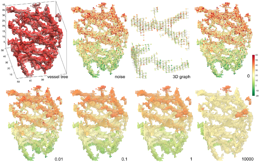
We applied heat kernel smoothing to the computed tomography (CT) of human lung obtained from DIR-lab dataset (https://www.dir-lab.com) [19, 20]. Super-resolution procedure was used to enhance the resolution from $1\times 1\times 2.5\mbox{ mm}^{3}$ to $1\times 1\times 1\mbox{ mm}^{3}$ resolution for CT images. The small part ($50\times 50\times 40$ voxels) of the CT image was used to illustrate the method and display the results better. The binary vessel segmentation was done using the multiscale Hessian filters at each voxel, as shown in the top left of Figure 3 [21, 22, 23].

The binary segmentation was converted into a 3D graph by taking each voxel as a node and connecting neighboring voxels. Using the 18-connected neighbor scheme, we connect two voxels only if they touch each other on their faces or edges. If voxels are only touching at their corner vertices, they are not considered as connected. Although we used the 18-connected neighbor scheme in this study, for visualization purpose only, Figure 3 displays the 6-connected neighbor scheme. This results in an adjacency matrix and the 3D graph Laplacian. Figure 3 example generates a 3D graph with $p=6615$ nodes. The center of voxel is taken as the node coordinates. The large-scale eigenvector problem was subsequently solved using an Implicitly Restarted Arnoldi Iteration method [24]. We used 6000 eigenvectors. Note we cannot have more eigenvectors than the number of nodes. Numbers in Figure 3 are kernel bandwidths. At $\sigma=0$, heat kernel smoothing is equivalent to Fourier series expansion. Thus, we get almost identical results. As the bandwidth increases, smoothing converges to the mean value. The regions that are different colors even with $\sigma=10000$ are regions that are disconnected. Thus, each disconnected regions are converging to their own different mean values.

Figure 4: The skeleton representation of vessel trees. Using the heat kernel series expansion with bandwidth $\sigma=1$ and 6000 basis, we upsampled the binary segmentation at 2, 4, 6 times (clockwise from top right) larger than the original size (top left).

VII Discussion

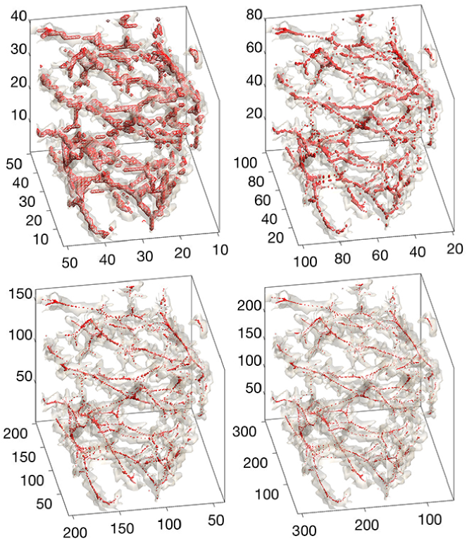
The proposed technique can be used to extract the skeleton representation of vessel trees. Here we show the proof of concept. We perform heat kernel smoothing on node coordinates with $\sigma=1$. Then rounded off the smoothed coordinates to the nearest integers. The rounded off coordinates were used to reconstruct the binary segmentation. This gives the thick trees in Figure 4 (top left). To obtain thinner trees, the smoothed coordinates were scaled by the factor of 2,4 and 6 times before rounding off. This had the effect of increasing the image size relative to the kernel bandwidth (Figure 4 clockwise from top right). We hope that our method offers a new way of making the skeleton representation of the vessel trees [16, 17].

References

- [1] M.K. Chung, S. Robbins, and A.C. Evans, “Unified statistical approach to cortical thickness analysis,” Information Processing in Medical Imaging (IPMI), Lecture Notes in Computer Science, vol. 3565, pp. 627–638, 2005.
- [2] M.K. Chung, S. Robbins, K.M. Dalton, R.J. Davidson, A.L. Alexander, and A.C. Evans, “Cortical thickness analysis in autism with heat kernel smoothing,” NeuroImage, vol. 25, pp. 1256–1265, 2005.
- [3] M.K. Chung, A. Qiu, S. Seo, and H.K. Vorperian, “Unified heat kernel regression for diffusion, kernel smoothing and wavelets on manifolds and its application to mandible growth modeling in CT images,” Medical Image Analysis, vol. 22, pp. 63–76, 2015.
- [4] X. Han, J. Jovicich, D. Salat, A. van der Kouwe, B. Quinn, S. Czanner, E. Busa, J. Pacheco, M. Albert, R. Killiany, et al., “Reliability of MRI-derived measurements of human cerebral cortical thickness: The effects of field strength, scanner upgrade and manufacturer,” NeuroImage, vol. 32, pp. 180–194, 2006.
- [5] G.M.L. Gladwell and H. Zhu, “Courant’s nodal line theorem and its discrete counterparts,” The Quarterly Journal of Mechanics and Applied Mathematics, vol. 55, pp. 1–15, 2002.
- [6] T. Tlusty, “A relation between the multiplicity of the second eigenvalue of a graph laplacian, courant’s nodal line theorem and the substantial dimension of tight polyhedral surfaces,” Electrnoic Journal of Linear Algebra, vol. 16, pp. 315–24, 2007.
- [7] Mikhail Belkin, Partha Niyogi, and Vikas Sindhwani, “Manifold regularization: A geometric framework for learning from labeled and unlabeled examples,” The Journal of Machine Learning Research, vol. 7, pp. 2399–2434, 2006.
- [8] J. Sun, M. Ovsjanikov, and L. J. Guibas, “A concise and provably informative multi-scale signature based on heat diffusion.,” Comput. Graph. Forum, vol. 28, pp. 1383–1392, 2009.
- [9] M. M. Bronstein and I. Kokkinos, “Scale-invariant heat kernel signatures for non-rigid shape recognition,” in IEEE Conference on Computer Vision and Pattern Recognition (CVPR), 2010, pp. 1704–1711.
- [10] F. de Goes, S. Goldenstein, and L. Velho, “A hierarchical segmentation of articulated bodies,” Computer Graphics Forum, vol. 27, pp. 1349–1356, 2008.
- [11] Bernhard Schölkopf and Alex J Smola, Learning with Kernels: Support Vector Machines, Regularization, Optimization, and Beyond, MIT Press, 2002.
- [12] J. Nilsson, F. Sha, and M.I. Jordan, “Regression on manifolds using kernel dimension reduction,” in Proceedings of the 24th international conference on Machine learning. ACM, 2007, pp. 697–704.
- [13] J Shawe-Taylor and N Cristianini, Kernel methods for pattern analysis, Cambridge University Press, 2004.
- [14] Florian Steinke and Matthias Hein, “Non-parametric regression between manifolds,” Advances in Neural Information Processing Systems, 2008.
- [15] F. Yger and A. Rakotomamonjy, “Wavelet kernel learning,” Pattern Recognition, vol. 44, no. 10-11, pp. 2614–2629, 2011.
- [16] L. Lindvere, R. Janik, A. Dorr, D. Chartash, B. Sahota, J.G. Sled, and B. Stefanovic, “Cerebral microvascular network geometry changes in response to functional stimulation,” Neuroimage, vol. 71, pp. 248–259, 2013.
- [17] L. Cheng, J. De, X. Zhang, F. Lin, and H. Li, “Tracing retinal blood vessels by matrix-forest theorem of directed graphs,” in International Conference on Medical Image Computing and Computer Assisted Intervention. Springer, 2014, pp. 626–633.
- [18] F.R.K. Chung and S.T. Yau, “Eigenvalue inequalities for graphs and convex subgraphs,” Communications in Analysis and Geometry, vol. 5, pp. 575–624, 1997.
- [19] R. Castillo, E. Castillo, R. Guerra, V.E. Johnson, T. McPhail, A.K. Garg, and T. Guerrero, “A framework for evaluation of deformable image registration spatial accuracy using large landmark point sets,” Physics in medicine and biology, vol. 54, pp. 1849–1870, 2009.
- [20] G. Wu, Q. Wang, J. Lian, and D. Shen, “Estimating the 4d respiratory lung motion by spatiotemporal registration and super-resolution image reconstruction,” Medical physics, vol. 40, no. 3, pp. 031710, 2013.
- [21] A.F. Frangi, W.J. Niessen, K.L. Vincken, and M.A. Viergever, “Multiscale vessel enhancement filtering,” in International Conference on Medical Image Computing and Computer-Assisted Intervention, 1998, vol. 1496, pp. 130–137.
- [22] P.D. Korfiatis, C. Kalogeropoulou, A.N. Karahaliou, A.D. Kazantzi, and L.I. Costaridou, “Vessel tree segmentation in presence of interstitial lung disease in MDCT,” IEEE Transactions on Information Technology in Biomedicine, vol. 15, pp. 214–220, 2011.
- [23] Y. Shang, R. Deklerck, E. Nyssen, A. Markova, J. de Mey, X. Yang, and K. Sun, “Vascular active contour for vessel tree segmentation,” IEEE Transactions on Biomedical Engineering, vol. 58, pp. 1023–1032, 2011.
- [24] R.B. Lehoucq and D.C. Sorensen, “Deflation techniques for an implicitly restarted arnoldi iteration,” SIAM Journal on Matrix Analysis and Applications, vol. 17, pp. 789–821, 1996.