Stochastic dark energy from inflationary quantum fluctuations

Abstract

We study the quantum backreaction from inflationary fluctuations of a very light, non-minimally coupled spectator scalar and show that it is a viable candiate for dark energy. The problem is solved by suitably adapting the formalism of stochastic inflation. This allows us to self-consistently account for the backreaction on the background expansion rate of the Universe where its effects are large. This framework is equivalent to that of semiclassical gravity in which matter vacuum fluctuations are included at the one loop level, but purely quantum gravitational fluctuations are neglected. Our results show that dark energy in our model can be characterized by a distinct effective equation of state parameter (as a function of redshift) which allows for testing of the model at the level of the background.

I Introduction

The origin of dark energy (DE) is one of the most fascinating unsolved problems of modern science. In literature traditionally two main classes of solutions have been proposed Joyce:2016vqv ; Gleyzes:2013ooa ; Bloomfield:2012ff ; Sahni:1999gb ; Sahni:2006pa ; Tsujikawa:2013fta ; Peebles:2002gy ; Baker:2012zs ; Bamba:2012cp :

1. matter condensates or physical DE, of which the simplest representatives are scalar condensates (quintessence models);

2. modified gravity or geometrical DE, which mimics dark energy by changing the relation between geometry and matter or by supplying additional geometric fields to general relativity.

However, there is no impenetrable barrier between these two possibilities, and more generically DE can be both physical and geometrical, i.e. a new matter field has to be introduced and gravity becomes modified, too. This just happens in the case of DE described by a non-minimally coupled scalar field considered in this paper. Recently the effective field theory (EFT) approach to dark energy Gubitosi:2012hu ; Bloomfield:2012ff ; Gleyzes:2013ooa has been developed. Its beauty is in that it presents a unified framework for both approaches, but its drawback is in that it does not immediately select the fundamental theory that lies behind some EFT. Nevertheless, different theories can be mapped onto the same class of EFTs, such that one can think of EFTs as identifying universality classes associated with DE models.

The question of naturalness of initial conditions is not addressed in traditional approaches. For example, in quintessence models typically a quintessence field starts running from a value which is not a (local or global) minimum of the potential. Criticisms are often brushed away by noting that similar malady plagues most of inflationary models. Arguably the main benefit of this work is in that we construct a theory that naturally explains the initial field value – which is accounted for by the calculable amplitude of infrared field fluctuations during inflation – thus addressing this fundamental criticism. The program advocated here can be thought of as a third way for understanding DE, in that in our class of models a link is established between primordial inflation and dark energy. This link, among other things, can be exploited when designing tests for these models.

Observers have devoted a lot of effort (and observational time) to nail down as accurately as possible the amount (and distribution) of dark energy. Since its discovery in 1998 Riess:1998cb ; Perlmutter:1998np a lot of progress has been made in improving the accuracy of DE measurements Suzuki:2011hu ; Parkinson:2012vd ; Palanque-Delabrouille:2014jca . At this moment the Planck satelite Ade:2015xua ; Ade:2015rim and the Dark Energy Survey (DES) Abbott:2017wau collaborations provide the most stringent bounds on dark energy. Presently $\Lambda$CDM, which assumes a cosmological constant equation of state $p\!=\!-\rho$ for dark energy, is consistent with all astronomical data. Assuming a general constant equation of state parameter $p\!=\!w\rho$ (the so-called $w$CDM model), combined Planck and Type Ia supernovae data provides constraints $w\!=\!-1.006\pm 0.045$ (68% CL).

Considering dynamical dark energy models – where $w$ that vary with redshift $z$ – yields significantly relaxed constraints Ade:2015rim . Still no statistically significant deviation of DE from an exact cosmological constant has been found . The upcoming measurements of Large Synoptic Survey Telescope (LSST) Abate:2012za , ESA’s Euclid satellite mission Amendola:2016saw and the European Extreme Large Telescope (E-ELT) Shearer:2010cn will further constrain dynamical DE models. For example, the accuracy of Euclid Amendola:2016saw is projected to be a few percent for simple (1 or 2 parameter models) and weaker for more involved models. Furthermore, these missions will be able to test some prominent DE models, including clustering of DE, growth of Universe’s structure, interactions of DE with itself and with other cosmological fluids, and – last but not least – the class of models presented here.

However, if the present DE traces its origin to a very early stage of the Universe, initial conditions for its subsequent evolution were quantum. As a result, it can remain quantum even up to the present time. Specifically in this work we investigate the influence of the quantum backreaction of a very light, nonminimally coupled spectator scalar field on the expansion dynamics of the Universe at late times. Our interest is to investigate what is the effect of inflationary quantum fluctuations that survive until late times and become comparable to – and eventually dominate over – the background nonrelativistic matter energy density driving the matter-dominated expansion. This idea goes back a while ago to Sahni:1998at ; Sahni:1999aq where it was noted that quantum fluctuations of a very light scalar could provide a CC-like contribution to the Friedmann equations. In recent years, similar ideas were examined Ringeval:2010hf ; Glavan:2013mra ; Aoki:2014ita ; Glavan:2014uga ; Aoki:2014dqa ; Glavan:2015cut . Most recently in Glavan:2015cut it was shown that, for certain ranges of model parameters, the backreaction remains small throughout the expansion of the Universe, and becomes relevant only at late times in matter era where it behaves approximately like a cosmological constant. Three parameters were introduced in this model: the total number of e-foldings of inflation $N_{I}$, the nonminimal coupling $\xi$, and the scalar field mass $m$. The conditions these parameters need to meet for the scenario to unfold are Glavan:2015cut

$$\Bigl{(}\frac{m}{H_{DE}}\Bigr{)}^{2}\ll 1\,,\qquad N_{I}<\frac{1}{8|\xi|}\ln\biggl{[}4\pi\Bigl{(}\frac{M_{P}}{H_{I}}\Bigr{)}^{2}\biggr{]}\,,\qquad 0>\xi>-\frac{1}{6}\Bigl{(}\frac{m}{H_{DE}}\Bigr{)}^{2}\,.$$ (1)

The first condition guarantees that the scalar field stays light throughout the expansion, the second one comes from requiring the backreaction to remain small (perturbative) during inflation, and the third one ensures that the leading term in the backreaction at very late times is of the cosmological constant type. Here $H_{I}$ is the inflationary Hubble rate, $H_{0}$ the Hubble rate today, and $H_{DE}$ the Hubble rate at the onset of dark energy domination. The magnitude of the cosmological constant today implies another relation that determines the total number of e-folding of inflation $N_{I}$ in terms of the remaining two parameters,

$$N_{I}=\frac{1}{8|\xi|}\ln\biggl{[}24\pi|\xi|\Bigl{(}\frac{M_{P}}{H_{I}}\Bigr{)}^{2}\Bigl{(}\frac{H_{DE}}{m}\Bigr{)}^{2}\biggr{]}\,.$$ (2)

It turns out this limits the range of the nonminimal coupling to $0>\xi\geq-10^{-2}$, and the number of total e-foldings of inflation is $N_{I}\gtrsim 10^{3}$.

In the regime where the backreaction becomes comparable to the background it can no longer be treated perturbatively, but rather its effects have to be taken into account properly by solving the semiclassical Friedmann equations self-consistently, with the quantum backreaction as a source. In general, these are rather complicated integro-differential equations. In principle these equations can be solved numerically by discretizing both the time evolution and the integral over the modes for the backreaction. An example of such computation was done in the context of reheating in Suen:1987gu , but it still presents a challenging numerical problem. Instead of the numerical approach we make use of the observation from the analytic computations Glavan:2015cut ; Glavan:2013mra ; Glavan:2014uga that the quantum backreaction for very light fields is dominated by the infrared (IR) modes not only during inflation, but throughout the history, and that the spectrum of these modes is inherited from the inflation era. The evolution of IR modes (which are largely amplified) during inflation (for small enough nonminimal coupling) is very accurately described by the formalism of stochastic inflation fully formulated in Starobinsky:1986fx (though some of its simplest applications were already used in Starobinsky:1982ee ). Here we adapt this method so that it becomes applicable to the evolution of IR modes in subsequent radiation and matter dominated eras of the Universe, and reproduce all the perturbative results of Glavan:2015cut . Such an approach to the problem was already advocated long ago in Sahni:1999gb , just after the original inception of the idea Sahni:1998at ; Sahni:1999aq , but – to our knowledge – it has not been carried out. We then use this method to approximate the semiclassical Friedmann equations in the regime where quantum backreaction is very large and write them as a closed set of differential equations which are much simpler to solve than the original integro-differential equations of semi-classical gravity. This approximation captures accurately the backreaction effects. These equations are then solved numerically. We find that the backreaction indeed accelerates the Universe, driving it towards a late de Sitter phase, very much like the observed behaviour of the Universe today, representing thus a novel dark energy candidate.

This paper is organized as follows. Section II presents the definition of the scalar field model and the standard cosmological history. In section III the stochastic formalism is derived for the model at hand, and in section IV the stochastic equations are solved in the regime of small backreaction and the results of Glavan:2015cut are reproduced. Section V presents the numerical solution of the full semiclassical Friedmann equations at late times, when backreaction is no longer small. In section VI we summarize and discuss the principal results.

II Scalar field in FLRW

In this section we define the cosmological background with the standard expansion history, on which our spectator scalar field model is defined and quantized.

II.1 FLRW background

The metric of the $D$-dimensional spatially flat Friedman-Lemaître-Robertson-Walker (FLRW) spacetime is given by

$$g_{\mu\nu}=\text{diag}(-1,a^{2}(t),\dots,a^{2}(t))$$ (3)

where $a$ is the scale factor, and the derivative of its logarithmic with respect to time defines the Hubble expansion rate, $H\!=\!\dot{a}/a$. The conventions that we use for the geometric quantities are $\Gamma^{\alpha}_{\mu\nu}=\frac{1}{2}g^{\alpha\beta}(\partial_{\mu}g_{\nu\beta}+\partial_{\nu}g_{\mu\beta}-\partial_{\beta}g_{\mu\nu})$ for the Christoffel symbol, $R^{\alpha}_{\mu\beta\nu}=\partial_{\beta}\Gamma^{\alpha}_{\mu\nu}-\partial_{\nu}\Gamma^{\alpha}_{\beta\mu}+\Gamma^{\rho}_{\mu\nu}\Gamma^{\alpha}_{\rho\beta}-\Gamma^{\rho}_{\mu\beta}\Gamma^{\alpha}_{\rho\nu}$ for the Riemann tensor, and $R_{\mu\nu}\!=\!{R^{\alpha}}_{\mu\alpha\nu}$ for the Ricci tensor. A convenient quantity we often use instead of time is the number of e-foldings $N$, which for the period between some $t_{0}$ and $t$ is equal to $N\!=\!\ln(a/a_{0})$.

The classical evolution of a spatially homogeneous, spatially flat universe is governed by the Friedmann equations,

$$H^{2}=\frac{2}{(D\!-\!1)(D\!-\!2)M_{\rm P}^{2}}\,\rho_{c}\,,\qquad\dot{H}=-\frac{1}{(D\!-\!2)M_{\rm P}^{2}}\,(\rho_{c}+p_{c})\,,$$ (4)

where $M_{\rm P}\!=\!(8\pi G)^{-1/2}\!\approx\!2.45\!\times\!10^{18}{\,\rm GeV}$ is the reduced Planck mass , $G$ is the Newton’s constant, and $\rho_{c}\!=\!\rho_{c}(t)$ and $p_{c}\!=\!p_{c}(t)$ are the classical pressure and energy density of the (dominant) cosmological fluid, respectively. Here we are primarily interested in solving for the Universe’s dynamics which also includes the quantum backreaction from inflationary quantum fluctuations of matter fields at the one-loop level. At the background level this approximation corresponds to what is known in the literature as semiclassical gravity, but the one-loop approximations goes beyond it since it includes higher order moments as well, so that background becomes stochastic effectively.

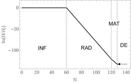
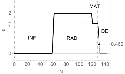
Large portions of the expansion history of the Universe are dominated by a single cosmological fluid with a constant equation of state. These periods are characterized by constant deceleration, or by a constant parameter $\epsilon\!=\!-\dot{H}/H^{2}$, where $\epsilon\!\approx\!0$ during inflation (where it is known as the slow-roll parameter), $\epsilon\!=\!2$ during radiation-dominated period, and $\epsilon\!=\!3/2$ during matter dominated period (see Fig. 1 for a schematic depiction of the evolution of $\epsilon$ parameter).

During $\epsilon\!=\!\text{const.}$ periods the scale factor and the Hubble rate evolve as

$$a(t)=a_{0}\bigl{[}1+\epsilon H_{0}(t\!-\!t_{0})\bigr{]}^{\frac{1}{\epsilon}}\,,\qquad H(t)=\frac{H_{0}}{1+\epsilon H_{0}(t\!-\!t_{0})}\,,$$ (5)

where $a_{0}$ and $H_{0}$ refer to the values at some particular time $t_{0}$, conveniently taken to be the beginning of a given constant $\epsilon$ period. The evolution of the Hubble rate is depicted schematically in Fig. 1.

Figure 1: Schematic evolution of the Hubble parameter (left), and the $\epsilon$ parameter (right) during the history of the Universe. The dot on the curves designates where we are today.

II.2 Nonminimally coupled massive scalar

The action for the nonminimally coupled scalar field in a curved background is

$$S[\Phi]=\int\!d^{D}x\,\mathcal{L}_{\Phi}=\int\!d^{D}\!x\,\sqrt{-g}\,\biggl{\{}-\frac{1}{2}g^{\mu\nu}\partial_{\mu}\Phi\partial_{\nu}\Phi-\frac{1}{2}m^{2}\Phi^{2}-\frac{1}{2}\xi R\Phi^{2}\biggr{\}}\,,$$ (6)

where $m$ is the scalar field mass, $R$ is the Ricci scalar, and $\xi$ is the nonminimal coupling with the sign convention where $\xi\!=\xi_{c}\!=(D\!-\!2)/[4(D\!-\!1)]\!\xrightarrow{D\rightarrow 4}\!{1}/{6}$ corresponds to the conformal coupling. We consider this model on an FLRW background.

In order to quantize the scalar field we first need to define the canonical formalism. The canonical momentum is

$$\Pi(x)=\frac{\partial\mathcal{L}_{\Phi}}{\partial\dot{\Phi}(x)}=a^{D-1}\dot{\Phi}(x)\ ,$$ (7)

and accordingly the Hamiltonian,

$$\text{H}[\Phi;t) = \int\!d^{D-1}x\,\Bigl{[}\Pi(t,\vec{x})\dot{\Phi}(t,\vec{x})-\mathcal{L}_{\Phi}(t,\vec{x})\Bigr{]}$$ (8)

$$= \int\!d^{D-1}x\,\biggl{\{}\frac{a^{1-D}}{2}\Pi^{2}+\frac{a^{D-3}}{2}\bigl{(}\vec{\nabla}\Phi\bigr{)}^{\!2}+\frac{a^{D-1}}{2}\Bigl{[}m^{2}+\xi(D\!-\!1)(D\!-\!2\epsilon)H^{2}\Bigr{]}\Phi^{2}\biggr{\}}\,.$$

Canonical quantization is now accomplished by promoting the field and its conjugate momentum to operators, and their Poisson brackets to equal-time commutation relations,

$$\bigl{[}\hat{\Phi}(t,\vec{x}),\hat{\Pi}(t,\vec{x}^{\,\prime})\bigr{]}=i\delta^{D-1}(\vec{x}\!-\!\vec{x}^{\,\prime})\,,\qquad\bigl{[}\hat{\Phi}(t,\vec{x}),\hat{\Phi}(t,\vec{x}^{\,\prime})\bigr{]}=0=\bigl{[}\hat{\Pi}(t,\vec{x}),\hat{\Pi}(t,\vec{x}^{\,\prime})\bigr{]}\,.$$ (9)

The Heisenberg equations of motion for the field operators are now,

$$\frac{d}{dt}\hat{\Phi}(t,\vec{x})-a^{1-D}\,\hat{\Pi}(t,\vec{x})=0\,,$$ (10)

$$a^{1-D}\,\frac{d}{dt}\hat{\Pi}(t,\vec{x})-\frac{\nabla^{2}}{a^{2}}\hat{\Phi}(t,\vec{x})+M^{2}(t)\,\hat{\Phi}(t,\vec{x})=0\,,$$ (11)

where the effective mass-squared is

$$M^{2}(t)=m^{2}+\xi R(t)=m^{2}+\xi(D\!-\!1)(D\!-\!2\epsilon)H^{2}\,.$$ (12)

It is convenient to expand the field operators in Fourier modes,

$$\hat{\Phi}(t,\vec{x}) = {\int}\!\!\frac{d^{D-1}k}{(2\pi)^{\frac{D-1}{2}}}\biggl{\{}e^{i\vec{k}\cdot\vec{x}}\varphi(t,k)\,\hat{b}(\vec{k})+e^{-i\vec{k}\cdot\vec{x}}\varphi^{*}(t,k)\,\hat{b}^{{\dagger}}(\vec{k})\biggr{\}}\,,$$ (13)

$$\hat{\Pi}(t,\vec{x}) = {\int}\!\!\frac{d^{D-1}k}{(2\pi)^{\frac{D-1}{2}}}\biggl{\{}e^{i\vec{k}\cdot\vec{x}}a^{D-1}\dot{\varphi}(t,k)\,\hat{b}(\vec{k})+e^{-i\vec{k}\cdot\vec{x}}a^{D-1}\dot{\varphi}^{*}(t,k)\,\hat{b}^{{\dagger}}(\vec{k})\biggr{\}}\,,$$ (14)

where the expansion of the conjugate momentum operator is such that it automatically satisfies Eq. (10). Observations tell us that the Universe is nearly spatially homogeneous on large scales. This motivates a spatially homogeneous Ansatz for the mode function $\varphi(t,k)$, where $k$ denotes the modulus of the comoving momentum $k\!=\!\|\vec{k}\|$, and the annihilation and creation operators, $\hat{b}$ and $\hat{b}^{{\dagger}}$, satisfy canonical commutation relations

$$\bigl{[}\hat{b}(\vec{k}),\hat{b}^{{\dagger}}(\vec{k}^{\,\prime})\bigr{]}=\delta^{D-1}(\vec{k}\!-\!\vec{k}^{\,\prime})\,,\qquad\bigl{[}\hat{b}(\vec{k}),\hat{b}(\vec{k}^{\prime})\bigr{]}=0=\bigl{[}\hat{b}^{{\dagger}}(\vec{k}),\hat{b}^{{\dagger}}(\vec{k}^{\prime})\bigr{]}\,.$$ (15)

This puts a constraint on the mode function in the form of a Wronskian normalization,

$$\varphi(t,k)\dot{\varphi}^{*}(t,k)-\dot{\varphi}(t,k)\varphi^{*}(t,k)=i\,a^{1-D}\,.$$ (16)

The equation of motion for the mode function inferred from (10-11) is

$$\ddot{\varphi}(t,k)+(D\!-\!1)H\dot{\varphi}(t,k)+\frac{k^{2}}{a^{2}}\varphi(t,k)+M^{2}(t)\,\varphi(t,k)=0\,.$$ (17)

The Hilbert space of states is constructed in the standard manner by defining a vacuum state $|\Omega\rangle$, which is annihilated by all the annihilation operators, $\hat{b}(\vec{k})|\Omega\rangle\!=\!0,\forall\vec{k}$. Then the rest of the state space is constructed by creation operators acting on $|\Omega\rangle$.

The energy-momentum tensor operator of the scalar field is given by

$$\hat{T}_{\mu\nu} = \frac{-2}{\sqrt{-g}}\frac{\delta S[\Phi]}{\delta g^{\mu\nu}}\Bigr{|}_{\Phi\rightarrow\hat{\Phi}}$$ (18)

$$= \partial_{\mu}\hat{\Phi}\,\partial_{\nu}\hat{\Phi}-\frac{1}{2}g_{\mu\nu}g^{\alpha\beta}\partial_{\alpha}\hat{\Phi}\,\partial_{\beta}\hat{\Phi}-\frac{m^{2}}{2}g_{\mu\nu}\hat{\Phi}^{2}+\xi\bigl{[}G_{\mu\nu}-\nabla_{\mu}\nabla_{\nu}+g_{\mu\nu}\square\bigr{]}\hat{\Phi}^{2}\,.$$

Its expectation value $\langle\cdot\rangle$ with respect to a homogeneous and isotropic state $|\Omega\rangle$ defined on a FLRW background (4) is diagonal and takes the form of ideal fluid,

$$\rho_{Q} = -\langle\hat{T}^{0}{}_{0}\rangle=\frac{1}{2}\langle(\partial_{0}\hat{\Phi})^{2}\rangle+\frac{1}{2a^{2}}\langle(\vec{\nabla}\Phi)^{2}\rangle+\frac{m^{2}}{2}\langle\hat{\Phi}^{2}\rangle$$ (19)

$$\hskip 85.35826pt+\xi\Bigl{[}\frac{1}{2}(D\!-\!1)(D\!-\!2)H^{2}+(D\!-\!1)H\partial_{0}\Bigr{]}\langle\hat{\Phi}^{2}\rangle\,,$$

$$p_{Q}\delta^{i}_{j} = \langle\hat{T}^{i}{}_{j}\rangle=\delta^{i}_{j}\biggl{\{}\frac{1}{2}\langle(\partial_{0}\hat{\Phi})^{2}\rangle-\frac{(D\!-\!3)}{2(D\!-\!1)a^{2}}\langle(\vec{\nabla}\hat{\Phi})^{2}\rangle-\frac{m^{2}}{2}\langle\hat{\Phi}^{2}\rangle$$ (20)

$$\hskip 71.13188pt-\xi\Bigl{[}\frac{1}{2}(D\!-\!2)\bigl{(}2\dot{H}+(D\!-\!1)H^{2}\bigr{)}+\partial_{0}^{2}+(D\!-\!2)H\partial_{0}\Bigr{]}\langle\hat{\Phi}^{2}\rangle\biggr{\}}\,,$$

where $\rho_{Q}\!=\!\rho_{Q}(t)$ and $p_{Q}\!=\!p_{Q}(t)$ are spatially homogeneous.

III Stochastic formalism

Here we briefly introduce the stochastic formalism of Starobinsky:1986fx for scalar fields in expanding cosmological space. The dominant contribution to the light scalar field correlators in inflation comes from the superhorizon modes (of wavelengths $k\!>\!1/aH$). This is also true for the very light or massless scalar fields in subsequent evolution of the Universe, namely during radiation and matter periods Glavan:2015cut ; Glavan:2014uga . The slow-roll approximation usually employed to derive the stochastic equations need not be correct in situations when the scalar becomes very massive, meaning $m\!\gtrsim\!H$. Since during decelerating periods of expansion the Hubble rate decays, this can eventually become true. This is why we do not use the slow-roll approximation in the stochastic formalism, but rather derive the equations for all three IR correlators. These reduce to the standard equations when the slow-roll hierarchy between the correlators is present.

III.1 Equations of motion for field operators

We split the field operators into the contributions from the long wavelength modes and from the short wavelength modes as follows,

$$\hat{\Phi}(t,\vec{x})=\hat{\phi}(t,\vec{x})+\hat{\phi}_{\text{s}}(t,\vec{x})\,,\qquad\hat{\Pi}(t,\vec{x})=\hat{\pi}(t,\vec{x})+\hat{\pi}_{\text{s}}(t,\vec{x})\,,$$ (21)

separated by a comoving scale $\mu aH$, where $0<\mu\!\ll\!1$ is the control parameter of the splitting. This splitting is most conveniently imposed in Fourier space where the long wavelength parts are

$$\hat{\phi}(t,\vec{x}) = {\int}\!\!\frac{d^{D-1}k}{(2\pi)^{\frac{D-1}{2}}}\,\theta\bigl{(}\mu aH\!-\!\|\vec{k}\|\bigr{)}\biggl{\{}e^{i\vec{k}\cdot\vec{x}}\varphi(t,k)\,\hat{b}(\vec{k})+e^{-i\vec{k}\cdot\vec{x}}\varphi^{*}(t,k)\,\hat{b}^{{\dagger}}(\vec{k})\biggr{\}}\,,$$ (22)

$$\hat{\pi}(t,\vec{x}) = {\int}\!\!\frac{d^{D-1}k}{(2\pi)^{\frac{D-1}{2}}}\,\theta\bigl{(}\mu aH\!-\!\|\vec{k}\|\bigr{)}\biggl{\{}e^{i\vec{k}\cdot\vec{x}}a^{D-1}\dot{\varphi}(t,k)\,\hat{b}(\vec{k})+e^{-i\vec{k}\cdot\vec{x}}a^{D-1}\dot{\varphi}^{*}(t,k)\,\hat{b}^{{\dagger}}(\vec{k})\biggr{\}}\,,\qquad$$ (23)

and the short wavelength parts

$$\hat{\phi}_{\text{s}}(t,\vec{x}) = {\int}\!\!\frac{d^{D-1}k}{(2\pi)^{\frac{D-1}{2}}}\,\theta\bigl{(}\|\vec{k}\|\!-\!\mu aH\bigr{)}\biggl{\{}e^{i\vec{k}\cdot\vec{x}}\varphi(t,k)\,\hat{b}(\vec{k})+e^{-i\vec{k}\cdot\vec{x}}\varphi^{*}(t,k)\,\hat{b}^{{\dagger}}(\vec{k})\biggr{\}}\,,$$ (24)

$$\hat{\pi}_{\text{s}}(t,\vec{x}) = {\int}\!\!\frac{d^{D-1}k}{(2\pi)^{\frac{D-1}{2}}}\,\theta\bigl{(}\|\vec{k}\|\!-\!\mu aH\bigr{)}\biggl{\{}e^{i\vec{k}\cdot\vec{x}}a^{D-1}\dot{\varphi}(t,k)\,\hat{b}(\vec{k})+e^{-i\vec{k}\cdot\vec{x}}a^{D-1}\dot{\varphi}^{*}(t,k)\,\hat{b}^{{\dagger}}(\vec{k})\biggr{\}}\,,\qquad$$ (25)

where, for simplicity, we took the Heaviside $\theta$-function for the window functions. We want to derive the analog of equations of motion (10) and (11), but just for the long wavelength parts of the field operators (22) and (23). Making use of the equation of motion (17) for the mode function the resulting equations are

$$\frac{d}{dt}\hat{\phi}(t,\boldsymbol{x})-a^{1-D}\,\hat{\pi}(t,\boldsymbol{x})=\hat{f}_{\phi}(t,\boldsymbol{x})\,,$$ (26)

$$a^{1-D}\,\frac{d}{dt}\hat{\pi}(t,\boldsymbol{x})-\frac{\nabla^{2}}{a^{2}}\hat{\phi}(t,\boldsymbol{x})+M^{2}(t)\,\hat{\phi}(t,\boldsymbol{x})=a^{1-D}\hat{f}_{\pi}(t,\boldsymbol{x})\,,$$ (27)

where the sources – which originate from the coupling between the short and long wavelength fields – are

$$\hat{f}_{\phi}(t,\vec{x}) = \mu aH^{2}(1\!-\!\epsilon){\int}\!\!\frac{d^{D-1}k}{(2\pi)^{\frac{D-1}{2}}}\,\delta\bigl{(}\|\vec{k}\|\!-\!\mu aH\bigr{)}\biggl{\{}e^{i\vec{k}\cdot\vec{x}}\varphi(t,k)\,\hat{b}(\vec{k})+e^{-i\vec{k}\cdot\vec{x}}\varphi^{*}(t,k)\,\hat{b}^{{\dagger}}(\vec{k})\biggr{\}}\,.$$ (28)

$$\hat{f}_{\pi}(t,\vec{x}) = \mu a^{D}H^{2}(1\!-\!\epsilon){\int}\!\!\frac{d^{D-1}k}{(2\pi)^{\frac{D-1}{2}}}\,\delta\bigl{(}\|\vec{k}\|\!-\!\mu aH\bigr{)}\biggl{\{}e^{i\vec{k}\cdot\vec{x}}\dot{\varphi}(t,k)\,\hat{b}(\vec{k})+e^{-i\vec{k}\cdot\vec{x}}\dot{\varphi}^{*}(t,k)\,\hat{b}^{{\dagger}}(\vec{k})\biggr{\}}\,.\qquad$$ (29)

The two sources (28) and (29) are to be considered as stochastic forces acting on the long wavelength fields, and here they originate from the effect of modes leaving (entering) the Hubble sphere due to accelerating (decelerating) expansion.

III.2 Equations of motion for IR correlators

Here we derive the equations for motion for the coincident long wavelength (infrared, IR) two-point functions, which we define to be conveniently rescaled,

$$\Delta_{\phi\phi}(t) \equiv \Bigl{\langle}\hat{\phi}^{2}(t,\vec{x})\Bigr{\rangle}\,,$$ (30)

$$\Delta_{\phi\pi}(t) \equiv \frac{1}{a^{3}(t)H(t)}\Bigl{\langle}\bigl{\{}\hat{\phi}(t,\vec{x}),\hat{\pi}(t,\vec{x})\bigr{\}}\Bigr{\rangle}\,,$$ (31)

$$\Delta_{\pi\pi}(t) \equiv \frac{1}{a^{6}(t)H^{2}(t)}\Bigl{\langle}\hat{\pi}^{2}(t,\vec{x})\Bigr{\rangle}\,.$$ (32)

The convenience of time dependent factors in the definitions above is in that all of these correlators become of the same dimension and the way they appear in the equations allows us to compare them directly which makes comparing their magnitudes straightforward. From now on we set $D\!=\!4$ since the UV divergences are captured by the short wavelength part of the fields. The equations of motion for these correlators follow from the equations of motion (26) and (27) for the long wavelength parts of the field operators (in $D\!=\!4$),

$$\frac{d}{dN}\Delta_{\phi\phi}-\Delta_{\phi\pi}=n_{\phi\phi}\,,$$ (33)

$$\frac{d}{dN}\Delta_{\phi\pi}+(3-\epsilon)\Delta_{\phi\pi}-2\Delta_{\pi\pi}+2\Bigl{(}\frac{M}{H}\Bigr{)}^{\!2}\Delta_{\phi\phi}=n_{\phi\pi}\,,$$ (34)

$$\frac{d}{dN}\Delta_{\pi\pi}+2(3-\epsilon)\Delta_{\pi\pi}+\Bigl{(}\frac{M}{H}\Bigr{)}^{\!2}\Delta_{\phi\pi}=n_{\pi\pi}\,,$$ (35)

In deriving these equations we have thrown away gradients, in particular terms of the form $\langle(\boldsymbol{\nabla}\phi)^{2}\rangle$, since they are suppressed by a factor of $\mu^{2}\!\ll\!1$ compared to the rest. This allows one to close the set of equations. Also we have switched to the number of e-foldings $N\!=\!\ln(a)$ as the time variable (with the choice of time (gauge) that corresponds to $a\!=\!1$ at the beginning of inflation), and $\epsilon\!=\!-\dot{H}/H^{2}$. The stochastic sources on the right hand side of (33–35) are the coincident field-noise correlators,

$$n_{\phi\phi} \equiv \frac{1}{H(t)}\Bigl{\langle}\bigl{\{}\hat{f}_{\phi}(t,\boldsymbol{x}),\hat{\phi}(t,\boldsymbol{x})\bigr{\}}\Big{\rangle}\,,$$ (36)

$$n_{\phi\pi} \equiv \frac{1}{a^{3}(t)H^{2}(t)}\biggl{[}\Bigl{\langle}\bigl{\{}\hat{f}_{\phi}(t,\boldsymbol{x}),\hat{\pi}(t,\boldsymbol{x})\bigr{\}}\Big{\rangle}+\bigl{\{}\hat{f}_{\pi}(t,\boldsymbol{x}),\hat{\phi}(t,\boldsymbol{x})\bigr{\}}\Big{\rangle}\biggr{]}\,,$$ (37)

$$n_{\pi\pi} \equiv \frac{1}{a^{6}(t)H^{3}(t)}\Bigl{\langle}\bigl{\{}\hat{f}_{\pi}(t,\boldsymbol{x}),\hat{\pi}(t,\boldsymbol{x})\bigr{\}}\Big{\rangle}\,.$$ (38)

These are straightforwardly computed from (22–23) and (28–29) to be

$$\Bigl{\langle}\bigl{\{}\hat{f}_{\phi}(t,\vec{x}),\hat{\phi}(t,\vec{x})\bigr{\}}\Bigr{\rangle} = \frac{1}{2\pi^{2}}\,\mu^{3}a^{3}H^{4}(1\!-\!\epsilon)\Bigl{[}|\varphi(t,k)|^{2}\Bigr{]}_{k=\mu aH}\,,$$ (39)

$$\Bigl{\langle}\bigl{\{}\hat{f}_{\phi}(t,\vec{x}),\hat{\pi}(t,\vec{x})\bigr{\}}\Bigr{\rangle} = \frac{1}{4\pi^{2}}\,\mu^{3}a^{6}H^{4}(1\!-\!\epsilon)\biggl{[}\frac{\partial}{\partial t}|\varphi(t,k)|^{2}\biggr{]}_{k=\mu aH}\,,$$ (40)

$$\Bigl{\langle}\bigl{\{}\hat{f}_{\pi}(t,\vec{x}),\hat{\phi}(t,\vec{x})\bigr{\}}\Bigr{\rangle} = \frac{1}{4\pi^{2}}\,\mu^{3}a^{6}H^{4}(1\!-\!\epsilon)\biggl{[}\frac{\partial}{\partial t}|\varphi(t,k)|^{2}\biggr{]}_{k=\mu aH}\,,$$ (41)

$$\Bigl{\langle}\bigl{\{}\hat{f}_{\pi}(t,\vec{x}),\hat{\pi}(t,\vec{x})\bigr{\}}\Bigr{\rangle} = \frac{1}{2\pi^{2}}\,\mu^{3}a^{9}H^{4}(1\!-\!\epsilon)\Bigl{[}|\dot{\varphi}(t,k)|^{2}\Bigr{]}_{k=\mu aH}\,,$$ (42)

where the anticommutator is defined as $\{\hat{A},\hat{B}\}\!\equiv\!\hat{A}\hat{B}\!+\!\hat{B}\hat{A}$, and where we have used that $\theta(0)\!=\!{1}/{2}$.  The sources (36-38) are referred to as the stochastic sources in analogy with the stochastic inflation formalism, though their physical interpretation during decelerating cosmological eras is not necessarily the one of standard stochastic sources. During decelerating eras ($\epsilon\!>\!1$) these sources have a negative overall sign, as evident from (39-42), and in fact contribute towards decreasing the correlators. This is not at all surprising if one notes that these sources arise as a time-dependent split of the modes into super-Hubble and sub-Hubble ones. During decelerated eras modes leak from the super-Hubble to sub-Hubble phase space (as opposed to accelerating periods where the leak is reversed) which accounts for the decrease in the IR correlators.

The energy density and pressure expectation values can be expressed in terms of the coincident IR correlators,

$$\rho_{Q} \approx \frac{H^{2}}{2}\biggl{\{}\Delta_{\pi\pi}+6\xi\Delta_{\phi\pi}+\Bigl{[}6\xi+\Bigl{(}\frac{m}{H}\Bigr{)}^{\!2}\Bigr{]}\Delta_{\phi\phi}\biggr{\}}\,,$$ (43)

$$p_{Q} \approx \frac{H^{2}}{2}\biggl{\{}(1\!-\!4\xi)\Delta_{\pi\pi}+2\xi\Delta_{\phi\pi}+\Bigl{[}-2\xi(3\!-\!2\epsilon)+24\xi^{2}(2\!-\!\epsilon)-\Bigl{(}\frac{m}{H}\Bigr{)}^{\!2}(1\!-\!4\xi)\Bigr{]}\Delta_{\phi\phi}\biggr{\}}\,.\qquad$$ (44)

The gradients were thrown away here on the same grounds as in the equations of motion (33-35) of the previous subsection. The short wavelength contributions were neglected since – after renormalization – except possibly during inflation, they contribute negligibly . These expressions for energy density and pressure can now be used to quantum-correct the Friedmann equations (in the sense that one should exact the replacements, $\rho_{c}\rightarrow\rho_{c}+\rho_{Q}$ and $p_{c}\rightarrow p_{c}+p_{Q}$ in (4)) and together with equations of motion (33-35) form a closed set of stochastic differential equations. It turns out that at late times (during radiation and matter era) stochastic sources contribute negligibly which will greatly simplify solving these equations.

IV Comparison with field theoretic calculations

Here we employ the stochastic formalism of the preceding section to calculate the backreaction of the scalar field quantum fluctuations during the three relevant cosmological periods and solve them perturbatively. These solutions are applicable in the regime where the quantum backreaction (43-44) is still negligible in comparison with the classical sources $\rho_{c}$ and $p_{c}$ in (4). The sources for the equations of motion (33–35) are determined using the mode functions from Glavan:2015cut . This section serves to reaffirm the results of Glavan:2015cut as well as to test the (perturbative) correctness of the stochastic formalism.

IV.1 De Sitter inflationary period

The results presented in this subsection were already derived in Finelli:2008zg ; Finelli:2010sh , both for test fields and for cosmological perturbations, and on the more general slow roll inflationary background.

The Chernikov-Tagirov-Bunch-Davies (CTBD) mode function of the scalar during the de Sitter inflation is

$$\varphi(t,k)=\sqrt{\frac{\pi}{4a^{3}H_{I}}}\ H_{\nu_{I}}^{(1)}\Bigl{(}\frac{k}{aH_{I}}\Bigr{)}\,,\qquad\nu_{I}=\sqrt{\tfrac{9}{4}-12\xi-\bigl{(}\tfrac{m}{H_{I}}\bigr{)}^{\!2}}\,.$$ (45)

where $H_{\nu}^{(1)}$ stands for the Hankel function of the first kind, and $H_{I}\!=\!{\rm const.}$ is the inflationary Hubble rate. This mode function coincides with the one of the adiabatic vacuum state for the subhorizon modes. The leading order IR expansion of the mode function (45) (for $k\!<\!\mu aH_{I}\!\ll\!aH_{I}$) is

$$\varphi(t,k)\approx\frac{(-i)}{\sqrt{\pi}}\,2^{\nu_{I}-1}\Gamma(\nu_{I})a^{\nu_{I}-3/2}H_{I}^{\nu_{I}-1/2}k^{-\nu_{I}}\,.$$ (46)

With this we can determine stochastic sources (36–38) for the equations of motion,

$$n_{\phi\phi}=\frac{2^{2\nu_{I}-3}}{\pi^{3}}\,\Gamma^{2}(\nu_{I})\mu^{3-2\nu_{I}}H_{I}^{2}\,,\quad n_{\phi\pi}=2\bigl{(}\nu_{I}\!-\!\tfrac{3}{2}\bigr{)}n_{\phi\phi}\,,\quad n_{\pi\pi}=\bigl{(}\nu_{I}\!-\!\tfrac{3}{2}\bigr{)}^{2}n_{\phi\phi}\,.$$ (47)

which are just constant. To leading order in nonminimal coupling and mass, $0\!<\!|\xi|,m^{2}/H_{I}^{2}\!\ll\!1$, they are independent of the separation scale $\mu$,

$$n_{\phi\phi}=\frac{H_{I}^{2}}{4\pi^{2}}\,,\qquad n_{\phi\pi}=-\frac{H_{I}^{2}}{6\pi^{2}}X\,,\qquad n_{\pi\pi}=\frac{H_{I}^{2}}{32\pi^{2}}X^{2}\,,$$ (48)

where the shorthand notation is $X\!=\!12\xi+(m/H_{I})^{2}$, and it is clear that $|X|\!\ll\!1$, which can be used as an expansion parameter, encompassing both minimally coupled and massive case. Parameter $X$ plays the role of an effective mass squared (in units of $H_{I}^{2}$) of the field during inflation. It can can take negative values $X<0$, signaling tachyonic particle production. This is not troubling, since the tachyonic nature of $X$ depends on the background spacetime, and is not present e.g. in flat space or in radiation era. 

The equations of motion for the coincident correlators (33-35) are now,

$$\frac{d}{dN}\Delta_{\phi\phi}-\Delta_{\phi\pi} = \frac{H_{I}^{2}}{4\pi^{2}}\,,$$ (49)

$$\frac{d}{dN}\Delta_{\phi\pi}+3\Delta_{\phi\pi}-2\Delta_{\pi\pi}+2X\Delta_{\phi\phi} = -\frac{H_{I}^{2}}{6\pi^{2}}X\,,$$ (50)

$$\frac{d}{dN}\Delta_{\pi\pi}+6\Delta_{\pi\pi}+X\Delta_{\phi\pi} = \frac{H_{I}^{2}}{36\pi^{2}}X^{2}\,.$$ (51)

The natural initial conditions for these equations are

$$\Delta_{\phi\phi}(0)=0\,,\qquad\Delta_{\phi\pi}(0)=0\,,\qquad\Delta_{\pi\pi}(0)=0\,.$$ (52)

These can be seen as arising from the set of modes which were initially super-Hubble ($k<\mu H_{I}$), meaning that initially the IR phase space is zero (this point we identify with the beginning of inflation at which $a=1$). This is not strictly speaking so, we rather assume that the super-Hubble modes at the beginning of inflation are suppressed due to some physical mechanism (for examples of how this can be done in practice see Janssen:2009nz ). In practice it is sufficient to assume that $\Delta_{\phi\phi}\!<\!H_{I}^{2}$ at the beginning of inflation. This results in them contributing subdominantly at late times.

Now the leading order solution in $|X|\!\ll\!1$ for these IR correlators is

$$\Delta_{\phi\phi}(N)=\frac{3H_{I}^{2}}{8\pi^{2}X}\Bigl{[}1-e^{-\frac{2}{3}XN}\Bigr{]}\,,\quad\Delta_{\phi\pi}(N)=-\frac{2X}{3}\Delta_{\phi\phi}(N)\,,\quad\Delta_{\pi\pi}(N)=\frac{X^{2}}{9}\Delta_{\phi\phi}(N)\,,$$ (53)

The subdominant contributions are suppressed by additional factors of $X^{3}$ compared to the leading order one , and also decay much faster with the number of e-foldings. Given the initial conditions (52), the stochastic sources determine the amplitude of the IR correlators. These sources also induce the hierarchy between the correlators which survives until very late times.

There are two interesting limits we discuss briefly in the two following subsections.

IV.1.1 Minimally coupled limit

The minimally coupled limit corresponds to taking $X\!=\!m^{2}/H_{I}^{2}$. There are two different cases to consider, the first one of which is the “long” inflation limit $N_{I}\!\gg\!(H_{I}/m)^{2}$, where the correlators eventually saturate to constant (de Sitter invariant) values,

$$\Delta_{\phi\phi}=\frac{3H_{I}^{2}}{8\pi^{2}}\Bigl{(}\frac{m}{H_{I}}\Bigr{)}^{\!\!-2}\,,\qquad\Delta_{\phi\pi}=-\frac{2}{3}\Bigl{(}\frac{m}{H_{I}}\Bigr{)}^{\!2}\Delta_{\phi\phi}\,,\qquad\Delta_{\pi\pi}=\frac{1}{9}\Bigl{(}\frac{m}{H_{I}}\Bigr{)}^{\!4}\Delta_{\phi\phi}\,.$$ (54)

The other case is the limit of “short” inflation $N_{I}\!\ll\!(H_{I}/m)^{2}$, where the correlators do not have enough time to saturate, and their values at the end of inflation are linear in the total number of e-foldings of inflation,

$$\Delta_{\phi\phi}(N_{I})=\frac{H_{I}^{2}}{4\pi^{2}}N_{I}\,,\qquad\Delta_{\phi\pi}(N_{I})=-\frac{2}{3}\Bigl{(}\frac{m}{H_{I}}\Bigr{)}^{\!2}\Delta_{\phi\phi}(N_{I})\,,\qquad\Delta_{\pi\pi}(N_{I})=\frac{1}{9}\Bigl{(}\frac{m}{H_{I}}\Bigr{)}^{\!4}\Delta_{\phi\phi}(N_{I})\,.$$ (55)

In both cases the hierarchy between the correlators is dictated by the small mass.

In the case of “long” inflation the energy density and pressure by the end of inflationary period are

$$\rho_{Q}=\frac{61H_{I}^{4}}{960\pi^{2}}\,,\qquad p_{Q}=-\rho_{Q}\,,$$ (56)

and in the case of “short” inflation they are

$$\rho_{Q}=-\frac{119H_{I}^{4}}{960\pi^{2}}+\frac{H_{I}^{2}m^{2}}{8\pi^{2}}N_{I}\,,\qquad p_{Q}=-\rho_{Q}\,.$$ (57)

Note that the contribution from the conformal anomaly $\rho_{CA}\!=\!-p_{CA}\!=\!-119H_{I}^{4}/(960\pi^{2})$ is included in both expressions since it is not negligible in these cases. In subsequent periods though, its contribution will be negligible. It should be noted that for our purposes the “long” inflation limit is extremely long (about $10^{13}$ efoldings), and the result (56) is computed under the assumption of exact de Sitter inflation (exactly flat plateau inflation). In cases of small deviations from such assumptions on inflation the scalar spectator does not necessarily reach stationary values for its correlators as pointed out in Hardwick:2017fjo , and one needs to be more careful when relating the correlator values of the spectator to the inflationary period history. What is of primary interest for us in this work is to establish that the scalar can attain super-Planckian correlator values by the end of inflation. The details of preciasely how it attains these values will introduce model dependent corrections to the relation (2) relating the number of e-foldings of inflation to the properties of the late time Universe.

IV.1.2 Massless limit

In the limit of negative nonminimal coupling which dominates over the mass term, $1\!\gg\!|\xi|\!\gg\!(m/H_{I})^{2}$, to leading order the field is effectively massless, and the correlators grow exponentially with the total number of e-foldings of inflation,

$$\Delta_{\phi\phi}(N_{I})=\frac{H_{I}^{2}}{32\pi^{2}|\xi|}\,e^{8|\xi|N_{I}}\,,\quad\Delta_{\phi\pi}(N_{I})=8|\xi|\,\Delta_{\phi\phi}(N_{I})\,,\quad\Delta_{\pi\pi}(N_{I})=16|\xi|\,\Delta_{\phi\phi}(N_{I})\,.$$ (58)

This growth of correlators during inflation is important for us for the model building of DE.

Note that in this case the leading order behavior of the correlators at late times in inflation is independent of the stochastic source, namely their growth is dominated by the instability of IR modes during inflation. Nevertheless, the stochastic sources, which in this case contribute significantly only during the beginning of inflationary period, fix the amplitude and the hierarchy of the correlators, accounting for the fact that all the contributing modes are of UV origin.

The energy density and pressure of the backreaction by the end of inflationary period in this case are

$$\rho_{Q}=-\frac{3H_{I}^{4}}{32\pi^{2}}\,e^{8|\xi|N_{I}}\,,\qquad p_{Q}=-\rho_{Q}\,.$$ (59)

IV.2 Radiation period

In radiation period we have $\epsilon_{R}\!=\!2$, so $a^{2}H\!=\!a_{1}^{2}H_{I}$, where $a_{1}$ refers to the value of the scale factor at the end of inflation/beginning of radiation. From Glavan:2015cut we have for the IR limit ($k\!<\!\mu aH\!\ll\!aH$) of the modulus squared of the scalar mode function,

$$|\varphi_{R}(t,k)|^{2}\approx\frac{4^{\nu_{I}-1}}{\pi}\Gamma^{2}(\nu_{I})\bigl{(}\nu_{I}\!-\!\tfrac{1}{2}\bigr{)}^{2}\frac{1}{a_{1}^{3}H_{I}}\Bigl{(}\frac{k}{a_{1}H_{I}}\Bigr{)}^{-2\nu_{I}}\Bigl{[}1-\frac{1}{10}\Bigl{(}\frac{m}{H}\Bigr{)}^{\!2}\,\Bigr{]}\,,$$ (60)

where the expression is valid up to the first subleading order in small mass. The other combinations of the mode function appearing in the stochastic sources can be determined from taking derivatives of the expression above, and by using the equation of motion (17). In particular,

$$|\dot{\varphi}_{R}(t,k)|^{2}=\frac{1}{2}\frac{d^{2}}{dt^{2}}|\varphi_{R}(t,k)|^{2}+\frac{3H}{2}\frac{d}{dt}|\varphi_{R}(t,k)|^{2}+m^{2}|\varphi_{R}(t,k)|^{2}\,,$$ (61)

where the gradient terms were dropped. The stochastic sources during radiation period, to leading order in $0\!\leq\!|\xi|,(m/H)^{2}\!\ll\!1$, are,

$$n_{\phi\phi}(N)\approx-\frac{H_{I}^{2}}{4\pi^{2}}\biggl{[}1-\frac{1}{10}\Bigl{(}\frac{m}{H}\Bigr{)}^{\!2}\,\biggr{]}\,,\quad n_{\phi\pi}(N)\approx\frac{H_{I}^{2}}{10\pi^{2}}\Bigl{(}\frac{m}{H}\Bigr{)}^{\!2}\,,\quad n_{\pi\pi}(N)\approx\mathcal{O}\Bigl{(}\frac{m}{H}\Bigr{)}^{\!\!4}\,.$$ (62)

The order $(m/H)^{2}$ to which the mode function was computed in Glavan:2015cut does not allow us to compute the leading order contribution to the last stochastic source above, but this is not important. Stochastic sources are relevant in inflation since they determine the amplitude of the correlators, but can actually safely be neglected in the subsequent periods of expansion. This argument can easily be made by examining the equations of motion,

$$\frac{d}{dN}\Delta_{\phi\phi}-\Delta_{\phi\pi} = n_{\phi\phi}\,,$$ (63)

$$\frac{d}{dN}\Delta_{\phi\pi}+\Delta_{\phi\pi}-2\Delta_{\pi\pi}+2\Bigl{(}\frac{m}{H}\Bigr{)}^{\!2}\Delta_{\phi\phi} = n_{\phi\pi}\,,$$ (64)

$$\frac{d}{dN}\Delta_{\pi\pi}+2\Delta_{\pi\pi}+\Bigl{(}\frac{m}{H}\Bigr{)}^{\!2}\Delta_{\phi\pi} = n_{\pi\pi}\,,$$ (65)

and by comparing the relative size of various terms. The final values of correlators at the end of inflation (55) or (58) serve as the initial conditions for the radiation period, and we note that both in minimally coupled, or massless limit they contain enhancement factors of $N_{I}$ or $e^{8|\xi|N_{I}}\!/|\xi|$, respectively. These derive partly from expanding the IR phase space of modes included in long wavelength correlators. On the other hand, none of the sources on the right hand side of (63)–(65) has this enhancement factor, making them negligible in comparison. Hence, to a very good approximation, the equations for IR correlators during (late) radiation era are the same as the classical ones,

$$\frac{d}{dN}\Delta_{\phi\phi}-\Delta_{\phi\pi} \approx 0\,,$$ (66)

$$\frac{d}{dN}\Delta_{\phi\pi}+\Delta_{\phi\pi}-2\Delta_{\pi\pi}+2\Bigl{(}\frac{m}{H}\Bigr{)}^{\!2}\Delta_{\phi\phi} \approx 0\,,$$ (67)

$$\frac{d}{dN}\Delta_{\pi\pi}+2\Delta_{\pi\pi}+\Bigl{(}\frac{m}{H}\Bigr{)}^{\!2}\Delta_{\phi\pi} \approx 0\,.$$ (68)

These equations we may solve perturbatively in small mass (and small nonminimal coupling contained in the initial conditions). To do this properly we need to take into account that the initial conditions of the radiation period satisfy the hierarchy inherited from inflation,

$$\Delta_{\phi\phi}(0)\gg\Delta_{\phi\pi}(0)\gg\Delta_{\pi\pi}(0)\,,$$ (69)

which is dictated by the same perturbative parameters. Therefore the equations that correctly capture the leading order correlators (denoted by superscript $(0)$) are

$$\frac{d}{dN}\Delta_{\phi\phi}^{(0)} = 0\,,$$ (70)

$$\frac{d}{dN}\Delta_{\phi\pi}^{(0)}+\Delta_{\phi\pi}^{(0)}+2\Bigl{(}\frac{m}{H}\Bigr{)}^{\!2}\Delta_{\phi\phi}^{(0)} = 0\,,$$ (71)

$$\frac{d}{dN}\Delta_{\pi\pi}^{(0)}+2\Delta_{\pi\pi}^{(0)}+\Bigl{(}\frac{m}{H}\Bigr{)}^{\!2}\Delta_{\phi\pi}^{(0)} = 0\,,$$ (72)

which we can readily solve,

$$\Delta_{\phi\phi}^{(0)}(N) = \Delta_{\phi\phi}(0)\,,$$ (73)

$$\Delta_{\phi\pi}^{(0)}(N) = \Delta_{\phi\pi}(0)e^{-N}-\frac{2}{5}\Delta_{\phi\phi}(0)\Bigl{(}\frac{m}{H}\Bigr{)}^{\!2}\Bigl{[}1\!-\!e^{-5N}\Bigr{]}\,,$$ (74)

$$\Delta_{\pi\pi}^{(0)}(N) = \Delta_{\pi\pi}(0)e^{-2N}+\frac{1}{25}\Delta_{\phi\phi}(0)\Bigl{(}\frac{m}{H}\Bigr{)}^{\!4}\Bigl{[}1\!-\!e^{-5N}\Bigr{]}^{2}-\frac{1}{5}\Delta_{\phi\pi}(0)\Bigl{(}\frac{m}{H}\Bigr{)}^{\!2}\Bigl{[}1\!-\!e^{-5N}\Bigr{]}e^{-N}\,.\qquad$$ (75)

This result encompasses both minimally coupled and massless limits.

At the end of radiation period (when $N_{R}\sim 50$) we can further simplify (73–75) by dropping the terms that have exponentially decayed,

$$\Delta_{\phi\phi}^{(0)}(N_{R}) = \Delta_{\phi\phi}(0)\,,$$ (76)

$$\Delta_{\phi\pi}^{(0)}(N_{R}) = \Delta_{\phi\pi}(0)e^{-N_{R}}-\frac{2}{5}\Delta_{\phi\phi}(0)\Bigl{(}\frac{m}{H_{\rm eq}}\Bigr{)}^{\!2}\,,$$ (77)

$$\Delta_{\pi\pi}^{(0)}(N_{R}) = \Delta_{\pi\pi}(0)e^{-2N_{R}}+\frac{1}{25}\Delta_{\phi\phi}(0)\Bigl{(}\frac{m}{H_{\rm eq}}\Bigr{)}^{\!4}\,,$$ (78)

where $N_{R}\!\approx\!50$ is the total number of e-foldings during radiation,  and $H_{\rm eq}$ is the Hubble rate at the end of radiation and beginning of matter period (radiation-matter equality). The energy density and pressure to leading order in radiation period are

$$\rho_{Q}\! = \!\frac{3H_{I}^{4}}{32\pi^{2}}e^{8|\xi|N_{I}}\biggl{[}-\Bigl{(}\frac{H}{H_{I}}\Bigr{)}^{2}+\frac{1}{6|\xi|}\Bigl{(}\frac{m}{H_{I}}\Bigr{)}^{2}\biggr{]}\,,$$ (79)

$$p_{Q}\! = \!\frac{3H_{I}^{4}}{32\pi^{2}}e^{8|\xi|N_{I}}\biggl{[}-\frac{1}{3}\Bigl{(}\frac{H}{H_{I}}\Bigr{)}^{2}-\frac{1}{6|\xi|}\Bigl{(}\frac{m}{H_{I}}\Bigr{)}^{2}\biggr{]}\,,$$ (80)

which is exactly what was obtained in Glavan:2015cut . There are two competing contributions in (79–80): a radiation-like fluid with negative energy and pressure, and a cosmological constant type contribution.

IV.3 Matter period

For the matter period the correlator values at the end of radiation (76)-(78) serve as initial conditions. Applying the same reasoning as in the radiation period case, the leading order equations of motion for the IR correlators in matter period are

$$\frac{d}{dN}\Delta_{\phi\phi}^{(0)} \approx 0\,,$$ (81)

$$\frac{d}{dN}\Delta_{\phi\pi}^{(0)}+\frac{3}{2}\Delta_{\phi\pi}^{(0)}+2\biggl{[}\Bigl{(}\frac{m}{H}\Bigr{)}^{\!2}+3\xi\biggr{]}\Delta_{\phi\phi}^{(0)} \approx 0\,,$$ (82)

$$\frac{d}{dN}\Delta_{\pi\pi}^{(0)}+3\Delta_{\pi\pi}^{(0)}+\biggl{[}\Bigl{(}\frac{m}{H}\Bigr{)}^{\!2}+3\xi\biggr{]}\Delta_{\phi\pi}^{(0)} \approx 0\,,$$ (83)

whose solutions are

$$\Delta_{\phi\phi}^{(0)}(N) = \Delta_{\phi\phi}(0)\,,$$ (84)

$$\Delta_{\phi\pi}^{(0)}(N) = \Delta_{\phi\pi}(0)e^{-3N/2}-4\xi\Delta_{\phi\phi}(0)\Bigl{[}1\!-\!e^{-3N/2}\Bigr{]}-\frac{4}{9}\Delta_{\phi\phi}(0)\Bigl{(}\frac{m}{H}\Bigr{)}^{\!2}\Bigl{[}1\!-\!e^{-9N/2}\Bigr{]}\,,$$ (85)

$$\Delta_{\pi\pi}^{(0)}(N) = \Delta_{\pi\pi}(0)e^{-3N}-\frac{2}{9}\Delta_{\phi\pi}(0)\Bigl{(}\frac{m}{H}\Bigr{)}^{\!2}\Bigl{[}1\!-\!e^{-9N/2}\Bigr{]}e^{-3N/2}-2\xi\Delta_{\phi\pi}(0)\Bigl{[}1\!-\!e^{-3N/2}\Bigr{]}e^{-3N/2}$$ (86)

$$+\frac{4}{81}\Delta_{\phi\phi}(0)\biggl{[}\Bigl{(}\frac{m}{H}\Bigr{)}^{\!2}\Bigl{[}1\!-\!e^{-9N/2}\Bigr{]}+9\xi\Bigl{[}1\!-\!e^{-3N/2}\Bigr{]}\biggr{]}^{2}\,.$$

Matter period lasts for about $N_{M}\!\approx\!8$ e-foldings before the onset of DE domination, so we can further simplify the results above,

$$\Delta_{\phi\phi}(N_{M}) = \Delta_{\phi\phi}(0)\,,$$ (87)

$$\Delta_{\phi\pi}(N_{M}) = 4\biggl{[}|\xi|-\frac{1}{9}\Bigl{(}\frac{m}{H}\Bigr{)}^{\!\!2}\,\biggr{]}\Delta_{\phi\phi}(0)\,,$$ (88)

$$\Delta_{\pi\pi}(N_{M}) = 4\biggl{[}|\xi|-\frac{1}{9}\Bigl{(}\frac{m}{H}\Bigr{)}^{\!\!2}\,\biggr{]}^{2}\Delta_{\phi\phi}(0)\,,$$ (89)

where $H_{\rm eq}>H\gg H_{DE}$ and $H_{DE}$ is the Hubble rate at the onset of DE domination, i.e. when $\rho_{c}=\rho_{Q}$. We see that the evolution preserves the hierarchy between the correlators induced by inflation, as long as the mass is smaller than the evolving Hubble rate. These we take as initial values for numerical evolution of the self-consistent quantum-corrected Friedmann equations.

The energy density and pressure in matter era has the same form as during radiation,

$$\rho_{Q}=\frac{3H_{I}^{4}}{32\pi^{2}}e^{8|\xi|N_{I}}\biggl{[}-\Bigl{(}\frac{H}{H_{I}}\Bigr{)}^{2}+\frac{1}{6|\xi|}\Bigl{(}\frac{m}{H_{I}}\Bigr{)}^{2}\biggr{]}\,,\qquad p_{Q}=\frac{3H_{I}^{2}}{32\pi^{2}}e^{8|\xi|N_{I}}\biggl{[}-\frac{1}{6|\xi|}\Bigl{(}\frac{m}{H_{I}}\Bigr{)}^{2}\biggr{]}\,,$$ (90)

confirming the results of Glavan:2015cut . Note that this expression is derived as a leading order contribution in the limit $0<-\xi\ll 1$ and $(m/H)^{2}\ll 1$. It does not quantitatively capture the limit $\xi\!=\!0$, in which case the enhancement factor $e^{8|\xi|N_{I}}$ takes a different form. Also, the case of a heavy scalar $(m/H)^{2}\gtrsim 1$ is not captured by these expressions, where the energy density and pressure of the scalar are of the nonrelativistic matter form at leading order.

There are two competing contributions in (90), one behaving like nonrelativistic matter (with negative energy), and the other one like a cosmological constant (CC). If the parameters of the model are such that the CC-like term starts dominating over the matter term before late times in matter era it should also eventually dominate over the background fluid and accelerate the expansion. This regime is beyond the (perturbative) regime discussed in the present section, where the backreaction on the expansion rate was neglected. It requires solving the set of semiclassical Friedman equations (4) (with $\rho_{c}\rightarrow\rho_{c}+\rho_{Q}$ and $p_{c}\rightarrow p_{c}+p_{Q}$) together with the matter era correlator equations self-consistently, as described at the end of section III. The expansion dynamics during that regime are determined in the next section.

V Self-consistent solution and results

Here we present solutions of the semiclassical Friedman equations with the initial conditions set during matter era at time $t=t_{*}$ when still $H(t_{*})=H_{*}\gg H_{DE}$. The quantum backreaction energy density and pressure (43–44) represent sources for the Friedman equations (4) on top of the classical matter fluid. The equations of motion for the correlators (33–35) with the sources neglected close the full set of equations.

$[m/H(z_{in})]^{2}=10^{-4},\ \xi=0$

$[m/H(z_{in})]^{2}=10^{-3},\ \xi=0$

Figure 2: Quantum backreaction model versus the $\Lambda$CDM model. Two columns represent two different choices of parameters $\xi$ and $m$. Left column: $[m/H(z_{in})]^{2}\!=\!10^{-4}$, $\xi\!=\!0$. Right column: $[m/H(z_{in})]^{2}\!=\!10^{-3}$, $\xi\!=\!0$. The first row shows plots of the Hubble rate, and the second row of the $\epsilon$ parameter in the backreaction model (solid line), and in the $\Lambda$CDM (dotted line). The third and fourth rows illustrate the difference between the Hubble rate and $\epsilon$ in the backreaction model and the $\Lambda$CDM model, respectively.

$[m/H(z_{in})]^{2}=10^{-4},\ \xi=-10^{-3}$

$[m/H(z_{in})]^{2}=10^{-3},\ \xi=-10^{-3}$

Figure 3: Quantum backreaction model versus the $\Lambda$CDM model. Two columns represent two different choices of parameters $\xi$ and $m$. Left column: $[m/H(z_{in})]^{2}\!=\!10^{-4}$, $\xi\!=\!-10^{-3}$. Right column: $[m/H(z_{in})]^{2}\!=\!10^{-3}$, $\xi\!=\!-10^{-3}$. The first row shows plots of the Hubble rate, and the second row of the $\epsilon$ parameter in the backreaction model (solid line), and in the $\Lambda$CDM (dotted line). The third and fourth rows illustrate the difference between the Hubble rate and $\epsilon$ in the backreaction model and the $\Lambda$CDM model, respectively.

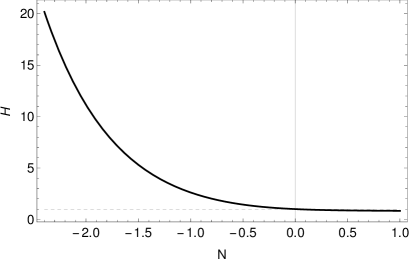
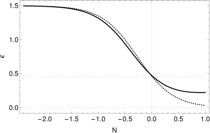
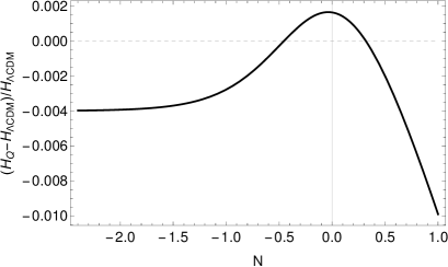
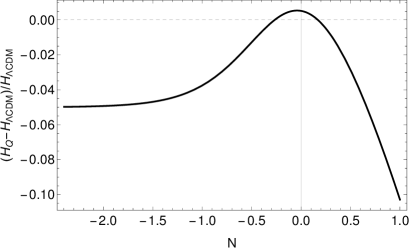
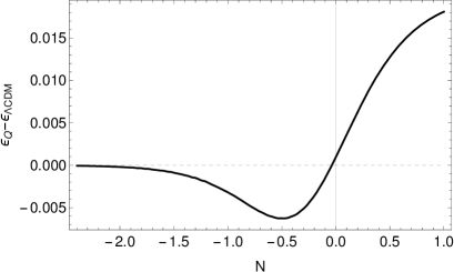
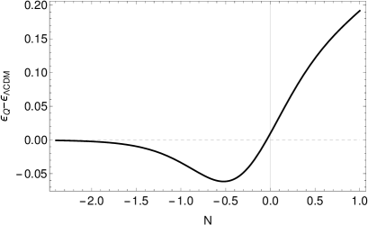
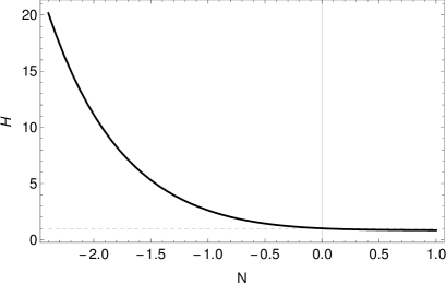
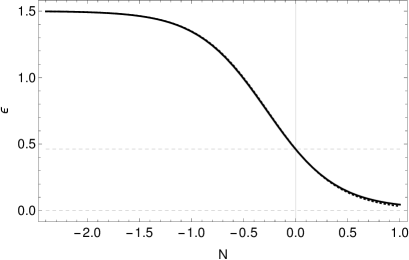
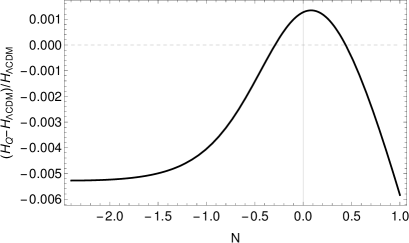
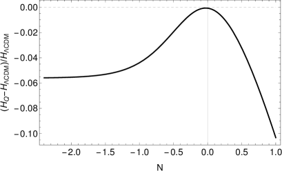
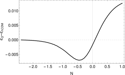
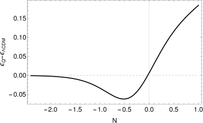
More specifically, initial conditions are set at redshift $z\!=\!z_{in}\!=\!10$ (corresponding to about 2 e-foldings in the past from today, $N(z)\!=\!-\ln(1\!+\!z)$) in such a way that the energy density and pressure of the would-be cosmological constant is substituted for the quantum backreaction. The equations are then solved numerically. The solutions for different choices of parameters are given in Figs. 2 and 3 which show how geometric quantities such as the Hubble rate $H$ and $\epsilon\!=\!(3/2)(1\!+\!w)$ (vertical axis) depend on the number of e-foldings $N=-\ln({1\!+\!z})$ (horizontal axis).

In Fig. 2 we see that, when $\xi\!=\!0$ and $m\!=\!0.20H_{0}$ [$m\!=\!0.01H(z\!=\!10)$], the relative difference between the Hubble expansion rate and $\epsilon$ in our model and $\Lambda$CDM is at a sub-percent level, which is not observable by current observations and at the verge of being observable by the near future observatories. However the differences become more pronounced when the scalar mass approaches the Hubble rate today. Indeed, when $m\simeq 0.61H_{0}$ [$m^{2}=10^{-3}H^{2}(z=10)$] the difference in the expansion rate and $\epsilon$ (or equivalently $w$) reaches several percent (see right panels in Fig. 2), which is testable by the next generation of observatories such as Euclid Amendola:2016saw and ELT Shearer:2010cn .

In order to study the effect of the nonminimal coupling $\xi$ on the geometrical quantities $H(z)$ and $\epsilon(z)$, in Fig. 3 we show the evolution of the Hubble parameter and $\epsilon$ as a function of the number of e-folding $N\!=\!-\ln({1\!+\!z})$ for $\xi\!=\!-10^{-3}$. As in Fig. 2 we see that for small masses, when $m\ll H_{0}$ ($m\simeq 0.20H_{0}$) the difference between $\Lambda$CDM and our model is at a sub-percent level and hence barely reachable by planned observatories. However, for a mass comparable to the Hubble rate today ($m\simeq 0.61H_{0}$), the difference becomes significant and well within reach of Euclid and ELT. Comparing Figs. 2 and 3 reveals that increasing $|\xi|$ seems to increase the difference between our model and $\Lambda$CDM. However, for small values of $\xi$’s ($\xi\!=\!-10^{-3}$ in figure 3) this increase is rather moderate. Note that a non-vanishing mass term (or a potential term) is crucial for the model to exhibit DE behaviour. (The case $m\!=\!0$ and $\xi\!<\!0$ is examined in Glavan:2014uga , and that model does not exhibit a late time dark energy.)

The nonminimal coupling is a relevant parameter here more from the point of view of relating the DE period to the primordial inflationary period, more precisely to the total number of e-foldings of inflation $N_{I}$. In case of zero nonminimal coupling this number has to be huge Aoki:2014dqa , $N_{I}\sim 10^{12}$ for both cases of Fig. 2, while for even rather small nonminimal couplings of Fig. 3 the total number of e-foldings of inflation is much smaller Glavan:2015cut , $N_{I}\sim 10^{5}$, which can be determined from (2). Larger values (in magnitude) for nonminimal coupling are problematic in the sense that one has to worry about large backreaction much earlier, during primordial inflation. Although this is an interesting possibility to study in the context of graceful exit from inflation, it is not considered in our DE model (for a recent study of the backreaction of a heavy nonminimally coupled scalar in de Sitter inflation see Markkanen:2016aes ).

$[m/H(z_{in})]^{2}=10^{-4},\ \xi=0$

$[m/H(z_{in})]^{2}=10^{-3},\ \xi=0$

$[m/H(z_{in})]^{2}=10^{-4},\ \xi=-10^{-3}$

$[m/H(z_{in})]^{2}=10^{-3},\ \xi=-10^{-3}$

Figure 4: The DE equation of state parameter $w_{DE}\equiv w_{Q}=p_{Q}/\rho_{Q}$ for the quantum backreaction as a function of $N\!=\!-\ln(1\!+\!z)$. To facilitate comparison, the parameters are chosen as in Fig. 2 and 3 and they are indicated above the plots. The uncertainty in the lower two plots reflects the uncertainty related to the subtraction of the part of the quantum backreaction that scales (to a good approximation) as dark matter. Note that the uncertainty is larger at larger redshift. However, that does not reduces in any significant way testability of the model, because at large redshifts the relative contribution of dark energy is small.

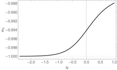
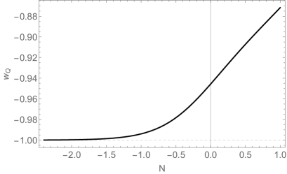
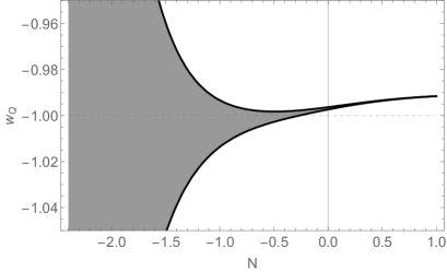
While Figs. 2 and 3 nicely show the recent Universe dynamics in our model and compare them to those of $\Lambda$CDM, it is instructive to show how the dark energy component in our model evolves, and that is illustrated in Fig. 4. The upper two plots show that for the vanishing nonminimal coupling ($\xi\!=\!0$), the backreaction behaves like a cosmological constant to a very good approximation in the late Universe, causing the transition from the matter-dominated to the quasi-de Sitter phase. This behaviour tends to persist until the Hubble rate drops below the mass scale of the scalar field ($m\!\sim\!H$). After this point the Universe transitions to a decelerated phase where $\epsilon$ oscillates between 0 and 3.

The lower two plots in Fig. 4 demonstrate the effect of non-minimal coupling on the dark energy equation of state. The shaded regions correspond to the uncertainty we have in estimating its equation of state. These are introduced for the following reason – due to nonminimal coupling the backreaction contains a contribution (whose energy density and pressure we denote as $\rho_{Q}^{m}$ and $p_{Q}^{m}$) that to a good approximation scales like nonrelativistic matter at higher redshifts (while the backreaction is still small), as is evident from Eq. (90). It is more appropriate not to consider this contribution a part of dark energy, but rather to group it together with the background matter fluid. Hence, we have subtracted the contribution from the backreaction that scales away exactly like mater, and determined the equation of state for the remaining contribution in the backreaction fluid. The uncertainty in $w_{Q}$ is due to the fact that the amplitude of this matter like contribution is computed approximately to order $\mathcal{O}(\xi)$, and that it does not scale exactly like matter, but its behaviour has corrections of the order of $\mathcal{O}(|\xi|N_{M})$, where $N_{M}$ is the number of e-foldings of the matter-dominated period. This means we do not know exactly how much of this matter-like fluid to subtract, which introduces sizeable uncertainties in the equation of state only for higher redshifts, but for smaller redshifts ($z\lesssim 3$) we get – up to sub-percent uncertainties – unique predictions. This implies that our model of dark energy is in principle testable as it gives a definite prediction for the equation of state parameter $w_{\rm Q}$ as a function of the redshift.

Even though we know that the subtracted matter-like contribution redshifts like ordinary matter on cosmological scales, we do not know how it clusters. If its clustering turns out to be insignificant, its principal effect would be a finite renormalization (reduction) of the Newton constant. In the opposite case the effect would fall under the class of some interacting dark matter/dark energy models, the precise nature of which requires further investigation, which is left for future work.

As of yet dark matter has not been directly seen. However, in the near future dark matter may be seen in the laboratories and if that happens, we may have enough to infer its energy density. Since our model predicts a negative component that redshifts as dark matter (see Eq. (90)), if it also clusters like dark matter, there should be more dark matter than what indirect observations (such as lensing) indicate. More concretely, for $[m/H(z_{in})]^{2}=10^{-4}$ and $\xi=10^{-3}$ the ratio is: $\rho_{Q}^{m}/\rho_{c}=-0.0687$ and for $[m/H(z_{in})]^{2}=10^{-3}$ $\xi=10^{-3}$ the ratio is $\rho_{Q}^{m}/\rho_{c}=-0.0085$, which is large enough to be potentially observable (both evaluated at redshift $z\simeq 10$). As far as we know, our model is the only one in the literature that exhibits this feature, which may become a smoking gun for testing our model.

$[m/H(z_{in})]^{2}=10^{-4},\ \xi=0$

$[m/H(z_{in})]^{2}=10^{-3},\ \xi=0$

$[m/H(z_{in})]^{2}=10^{-4},\ \xi=-10^{-3}$

$[m/H(z_{in})]^{2}=10^{-3},\ \xi=-10^{-3}$

Figure 5: The DE equation of state parameter $w_{DE}$ as a function of $N\!=\!-\ln(1\!+\!z)$. The solid black curve shows the quantum backreaction equation of state parameter, $w_{Q}(N)$, the dashed curve shows $w_{DE}(N)$ in the $w_{0}w_{a}$CDM model, in which $w_{DE}(N)\!=\!w_{0}+(1\!-\!e^{N})w_{a}$, and the shaded region is the $1\sigma$ contour corresponding to $w_{0}\!=\!-0.6\pm 0.25$, $w_{a}\!=\!-0.3\pm 0.8$.

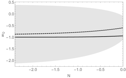
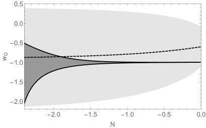
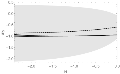
Let us now compare with current observations. The Planck collaboration papers Ade:2015xua ; Ade:2015rim constrain $w_{DE}=-1.019{+0.075\atop-0.080}$ ($68\%$ CL when the complete Planck data are combined with available data from lensing, baryonic acoustic oscillations (BAO) and $H_{0}$ measurements). On the other hand, the $68\%$ CL error bars on the parameters of the $w_{0}w_{a}$CDM model [defined by, $w_{DE}=w_{0}+(1-a)w_{a}=w_{0}+[z/(1+z)]w_{a}=w_{0}+(1-e^{N})w_{a}$] are much weaker, $w_{0}=-0.6\pm 0.25,w_{a}=-0.3\pm 0.8$ (with the Planck, BAO, SN-Ia $\&$ $H_{0}$ data included) and $w_{0}=-0.6\pm 0.5,w_{a}=-1.2\pm 1.2$ (with the Planck, BAO $\&$ redshift space distortions data included) (see figure 4 in Ref. Ade:2015rim ), which shows that the constraints $w_{0}$ and $w_{a}$ depend significantly on the data sets used and hence the quality of the data is still not good enough to place strong bounds on the model. Since these bounds are only slightly modified when the more recent 1 year DES data are accounted for Abbott:2017wau , they suffice for our purpose. It is clear that these bounds are not precise enough to place meaningful constraints on the dark energy models shown in Fig. 4. This can be seen even clearer in Fig. 5, in which we observe that the contours of our dark energy model lie comfortably within one standard deviation contours of the $w_{0}w_{a}$CDM model (which meaningfully constrains dark energy only at relatively small redshifts, $z\lesssim 2$, or $N\gtrsim-1$).

However, with the incipience of upcoming high precision observatories such as Euclid and LSST, the constraints may become strong enough to curb our model, especially when combined with inhomogeneous probes.

VI Discussion and outlook

This paper is one in a series Glavan:2013mra ; Glavan:2014uga ; Glavan:2015cut , whose goal is to investigate viability of DE models based on quantum fluctuations during inflation. The attractiveness of these models stems from the fact that – when compared to more conventional DE models – they are amenable to additional tests. For example, since the origin of these models can be traced back to inflation, there is an intricate relationship between DE and infationary observables. Furthermore, since the origin of DE in these models is in quantum fluctuations of matter fields, in general we expect these models to generate inhomogeneous dark energy with calculable amount of inhomogeneities, which can also be used to test this class of models.

In this paper we reanalyze the dark energy model proposed in Ref. Glavan:2015cut . The model utilizes an ultra-light, non-minimally coupled scalar field and its dynamics is governed by the action (6). Even though this field is a spectator field during inflation, quantum fluctuations naturally grow large such that, by the end of inflation, they typically reach super-Planckian values. In fact, due to the assumed negative non-minimal coupling, it can take as little as a thousand of e-foldings to achieve this feat. This mechanism addresses the question of naturalness of initial conditions – often raised in quintessence DE models – by dynamically generating super-Planckian fluctuations from initially subhorizon quantum fluctuations.

In order to be able to calculate beyond the perturbative regime of Ref. Glavan:2015cut , in section III we develop a stochastic framework which permits us to solve the problem self-consistently, also in the regime where the quantum backreaction dominates the background dynamics. To establish the accuracy of our stochastic model, in section IV we use the stochastic framework to calculate the one loop contribution to the energy density and pressure of quantum fluctuations and demonstrate agreement with the perturbative calculations of Ref. Glavan:2015cut in all of the relevant epochs: inflation, radiation and matter era. This is sufficient to establish perturbative accuracy of the model. The main advantage of the stochastic formulation is in that a self-consistent solution of semiclassical gravity comes within reach of even modest programmers, as the original set of integro-differential equations of semiclassical gravity is reduced to a much simpler set of ordinary differential equations with rather facile stochastic sources.

A notable result of our work is that stochastic sources – which are of essential importance for capturing the correct dynamics during inflation – can be neglected during the post-inflationary radiation and matter epochs, such that the field dynamics becomes essentially classical. The memory of stochastic sources is still kept in the initial conditions for radiation era and for matter era.

Armed with this formalism we then study how quantum inflationary fluctuations in our model (6) evolve in time and how they affect the background evolution. In particular in Fig. 2 and 3 we compare the evolution of the Hubble rate $H(t)$ and its dimensionless rate of change, $\epsilon\!=\!-\dot{H}/H^{2}$ (which is equal to the principal slow roll parameter during inflation) in our model with the same in $\Lambda$CDM. Our results show that, as the ultra-light mass $m$ is taken to be closer to, but still remains smaller than, the Hubble parameter today, the differences become significant and observable by the near future observatories such as Euclid and ELT. From Figs. 4 and 5 we see that the current data are not constraining enough to meaninfully test our the backreaction DE models. However, the near future data (from Euclid, SST, ELT and other planned observatories) will penetrate deeper into the redshift space and will be collecting much more data and thus will be able to constrain the quantum backreaction DE models. Next, we point out that the dependence of $w_{Q}=w_{Q}(z)$ in our quantum backreaction model is quite different from that in typical quintessence models Tsujikawa:2013fta . This owes to the rather unusual feature of the perturbative initial condition in matter era (79–80), which is in turn dictated by the standard (IR-regulated) Chernikov-Tagirov-Bunch-Davies initial condition in inflation (45). Namely, there is a significant negative energy component that initially scales as the dominant background (dark matter) component (cf. Eqs. (79–80)). This feature is akin to negative energy scenarios studied in Prokopec:2011ce and – once the properties of (particle-like) dark matter are mapped out – can be used to test this class of DE models.

While in this paper we only study the background evolution, keeping in mind the quantum inflationary origin of scalar field dark energy in our model, it would be of utmost importance to investigate the growth of structure in the visible and dark energy sector in our DE model, both at Gaussian and non-Gaussian levels. Namely, due to the non-minimal coupling the model is non-Gaussian and hence we expect it to leave distinct Gaussian and non-Gaussian footprints at late times on Universe’s large scale structure. Determining these will require a suitable adaptation of the stochastic formalism for off-coincident correlation functions in inflation Starobinsky:1994bd or of further developments in the stochastic $\delta N$ formalism used in Fujita:2014tja ; Pattison:2017mbe .

From the theoretical point of view, the model we presented here addresses the issue of naturalness of initial conditions, but there still remains the issue of fine-tuning in the form of requiring the scalar to have a tiny mass $m\leq H_{0}$. This issue is not specific to our model, but is a generic feature of all classical quintessence models. It would be of great interest to investigate whether a similar effect can be reproduced within different (interacting) models, via a mechanism that utilises spontaneous symmetry breaking Frieman:1995pm or ’t Hooft’s naturalness hypothesis tHooft:1979rat .