2D wind clumping in hot, massive stars from hydrodynamical line-driven instability simulations using a pseudo-planar approach

Abstract

Context. Clumping in the radiation-driven winds of hot, massive stars arises naturally due to the strong, intrinsic instability of line-driving (the ‘LDI’). But LDI wind models have so far mostly been limited to 1D, mainly because of severe computational challenges regarding calculation of the multi-dimensional radiation force.

Aims. To simulate and examine the dynamics and multi-dimensional nature of wind structure resulting from the LDI.

Methods. We introduce a ‘pseudo-planar’, ‘box-in-a-wind’ method that allows us to efficiently compute the line-force in the radial and lateral directions, and then use this approach to carry out 2D radiation-hydrodynamical simulations of the time-dependent wind.

Results. Our 2D simulations show that the LDI first manifests itself by mimicking the typical shell-structure seen in 1D models, but how these shells then quickly break up into complex 2D density and velocity structures, characterized by small-scale density ‘clumps’ embedded in larger regions of fast and rarefied gas. Key results of the simulations are that density-variations in the well-developed wind statistically are quite isotropic and that characteristic length-scales are small; a typical clump size is $\ell_{\rm cl}/R_{\ast}\sim 0.01$ at $2R_{\ast}$, thus resulting also in rather low typical clump-masses $m_{\rm cl}\sim 10^{17}$ g. Overall, our results agree well with the theoretical expectation that the characteristic scale for LDI-generated wind-structure is of order the Sobolev length $\ell_{\rm Sob}$. We further confirm some earlier results that lateral ‘filling-in’ of radially compressed gas leads to somewhat lower clumping factors in 2D simulations than in comparable 1D models. We conclude by discussing an extension of our method toward rotating LDI wind models that exhibit an intriguing combination of large- and small-scale structure extending down to the wind base.

1 Introduction

For massive, hot stars of spectral types OBA, scattering and absorption in spectral lines transfer momentum from the star’s intense radiation field to the plasma, and so provide the force necessary to overcome gravity and drive a strong stellar wind outflow (see Puls et al., 2008, for an extensive review). The first quantitative description of such line-driving was given in the seminal paper by Castor et al. (1975): hereafter ‘CAK’. Like many wind models to date, CAK used the so-called Sobolev approximation (Sobolev, 1960) to compute the radiative acceleration. This assumes that hydrodynamic flow quantities are constant over a few Sobolev lengths $\ell_{\rm Sob}=\varv_{\rm th}/(d\varv_{\rm n}/dn)$ (for ion thermal speed $\varv_{\rm th}$ and projected velocity gradient $d\varv_{\rm n}/dn$ along a coordinate direction $\hat{n}$), allowing then for a local treatment of the line radiative transfer.

Such a Sobolev approach ignores the strong ‘line deshadowing instability’ (LDI) that occurs on scales near and below the Sobolev length (Owocki & Rybicki, 1984); numerical radiation-hydrodynamic modeling of the non-linear evolution of the LDI shows that the time-dependent wind develops a very inhomogeneous, ‘clumped’ structure (Owocki et al., 1988; Feldmeier et al., 1997; Dessart & Owocki, 2003, 2005a; Sundqvist & Owocki, 2013, 2015). Such clumpy LDI models provide a natural explanation for a number of observed phenomena in OB-stars, such as the soft X-ray emission and broad X-ray lines observed by orbiting telescopes like chandra and xmm-newton (Feldmeier et al., 1997; Berghoefer et al., 1997; Güdel & Nazé, 2009; Cohen et al., 2010; Martínez-Núñez et al., 2017), the extended regions of zero residual flux typically seen in saturated UV resonance lines (Lucy, 1983; Puls et al., 1993; Sundqvist et al., 2010), and the migrating spectral sub-peaks superimposed on broad optical recombination lines (Eversberg et al., 1998; Dessart & Owocki, 2005b; Lépine & Moffat, 2008).

But a severe limitation of most of the above-mentioned models is their assumed spherical symmetry. The fact that most LDI simulations in the past have been limited to 1D is mainly a consequence of the computational cost associated with carrying out the non-local integrals needed to compute the radiation acceleration at each simulation time-step, while simultaneously resolving length-scales below $\ell_{\rm Sob}$. Specifically, following the general escape-integral methods developed by Owocki & Puls (1996), some $n_{\rm x}\approx 3\varv_{\infty}/\varv_{\rm th}\approx 1000$ discrete frequency points are typically needed to properly resolve line profiles and model the expanding flow. In 2D or 3D, a proper treatment of the multi-dimensional wind further requires integrations along a set of oblique rays in order to compute the radiative force in the radial and lateral directions. A major issue then becomes misalignment of nonradial rays with the discrete numerical grid (i.e. that oblique ray-integrations from any given point in the mesh in general do not intersect any other point), requiring that all integrations be repeated for each grid node (and also then involving complex interpolation schemes to trace the rays).

As an explicit example (see also Dessart & Owocki 2005a), for a 2D grid of $n_{\rm r}$ radial and $n_{\phi}$ azimuthal points, one needs $n_{\rm r}n_{\phi}$ integrations of order $n_{\rm r}n_{\rm x}$ operations for every considered ray; this gives an overall scaling $n_{\rm ray}n_{\rm x}n_{\rm r}^{2}n_{\phi}$, implying for a typical case of $n_{\rm ray}\approx 5$, $n_{\phi}\approx 100$, and $n_{\rm x}\approx n_{\rm r}\approx 1000$ on order $10^{11-12}$ operations to evaluate the radiative force. Moreover, such a calculation has to be carried out at each time-step of the hydrodynamical simulation, which for a typical courant time $\sim 5$ sec in a hot-star wind outflow, and a total simulation-time of, say, $\sim 50$ dynamical time scales $t_{\rm dyn}=R_{\ast}/\varv_{\infty}\sim 10$ ksec, requires some $\sim 10^{5}$ repeated evaluations of the radiative force. This simple example thus illustrates quite vividly the rather daunting task of constructing multi-dimensional LDI wind models.

Nonetheless, a few previous attempts have been performed. Dessart & Owocki (2003) carried out ‘2D hydro+1D radiation’ simulations by simply focusing only on the line force from a single radial ray, thus ignoring lateral influences. This led then to extensive break-up of the spherical shells seen in 1D simulations, resulting in lateral incoherence all the way down to the grid-scale. However, these simulations ignore the lateral component of the diffuse radiative force, which linear stability analysis (Rybicki et al., 1990) shows could lead to damping of velocity variations at scales below the lateral Sobolev length $\ell_{\rm Sob}=r\varv_{\rm th}/\varv$ and as such to more lateral coherence than seen in the single-ray 2D simulations. Dessart & Owocki (2005a) made a first attempt to include oblique rays, by using a special, restricted numerical grid in a 2D plane that forced 3 rays to always intersect the discrete mesh points (Owocki, 1999). But while these simulations did seem to suggest a somewhat larger lateral coherence than comparable 1-ray models, the inherent limitations of the method (e.g. in resolving the proper lateral scales) left results uncertain (Dessart & Owocki, 2005a).

This paper introduces a ‘pseudo-planar’ modeling approach for a multi-dimensional wind subject to the LDI. In this ‘box-in-a-wind’ method, all sphericity effects of the expanding flow are included in a radial direction $r$, but some curvature terms are ignored in the lateral direction(s). As discussed in §2 (and detailed in Appendix A), for a 2D simulation in the $r,y$ plane this allows us to consider 5 ‘long characteristic’ rays with a computational cost-scaling $3n_{\rm x}n_{\rm r}n_{\rm y}$, thus reducing the general scaling above with a factor $\sim n_{\rm r}=1000$ for our standard set-up. Using this method, §3 examines the resulting 2D clumpy wind structure in much greater detail than possible before, and §4 discusses the results, compares to other simulation test-runs, and outlines future work.

2 Modeling

The simulations here use the numerical PPM (Colella & Woodward, 1984) hydrodynamics code VH-1 to evolve the conservation equations of mass and momentum for a 2D, isothermal line-driven stellar wind outflow. A key point of this paper is that while we keep all sphericity effects of an expanding outflow in the radial direction, we neglect some curvature terms in the lateral direction(s); for details, see Appendix A. Preserving all properties of a spherical outflow, this pseudo-planar, box-in-a-wind approach allows us to resolve laterally the relevant clump-length-scales, as well as implement non-radial rays for the radiative line-driving in a time-efficient way (see further below and Appendix A).

All presented results adopt the same stellar and wind parameters as in Sundqvist & Owocki (2013, 2015), given here in Table 1, which are typical for an O-star in the Galaxy. The standard set-up uses a spatial grid with 1000 discrete radial ($r$) mesh-points between $R_{\ast}\leq r\leq 2R_{\ast}$ and 100 lateral ($y$) ones that cover in total $0.1R_{\ast}$. As such, the grid is uniform and has a constant step-size $\Delta=0.001R_{\ast}$; a small $\Delta$ is required to resolve both the sub-sonic wind-base with effective scale height $H=a^{2}R_{\ast}^{2}/(GM_{\ast}(1-\Gamma_{\rm e}))\approx 0.002R_{\ast}>\Delta$ and the resulting small-scale 2D clump structures in the supersonic wind (the focus of this paper). Each simulation evolves from a smooth, CAK-like initial condition, computed by relaxing to a steady state a 1D spherically symmetric time-dependent simulation that uses a CAK/Sobolev form for the line-force. To prevent artificial structure due to numerical truncation errors we use an evolution time-step that is the minimum of a fixed 2.5 sec and a variable 1/3 of the courant time (see discussion in Poe et al. 1990). As in previous work, the lower boundary at the assumed stellar surface fixes the density to a value $\sim 5-10$ times that at the sonic point. Moreover, since we are interested in structures that are considerably smaller than the computational box, the lateral boundaries are simply treated as periodic.

Table 1: Summary of stellar and wind parameters

Name	Parameter	Value
Stellar luminosity	$L_{\ast}$	$8\,\times\,10^{5}\,\rm L_{\odot}$
Stellar mass	$M_{\ast}$	50  $\rm M_{\odot}$
Stellar radius	$R_{\ast}$	20  $\rm R_{\odot}$
Isoth. sound speed	$a$	23.4 km/s
Average
- wind speed at $2R_{\ast}$	$\langle\varv_{\rm max}\rangle$	1230 km/s
- mass-loss rate	$\langle\dot{M}\rangle$	$1.3\,\times\,10^{-6}\,\rm M_{\odot}/yr$
CAK exponent	$\alpha$	0.65
Line-strength
- normalization	$\bar{Q}$	2000
- cut-off	$Q_{\rm max}$	0.004$\bar{Q}$
Ratio of ion thermal
speed to sound speed	$\varv_{\rm th}/a$	0.28
Eddington factor	$\Gamma_{\rm e}=$	0.42
	$\kappa_{\rm e}L_{\ast}/(4\pi GM_{\ast}c)$

2.1 Radiative driving

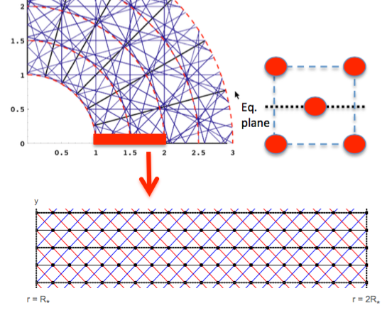
Figure 1: Sketch illustrating the basic idea of the pseudo-planar, box-in-a-wind approach used in this paper. The upper left illustrates the general situation of non-alignment between oblique rays and the numerical grid points. The lower panel then shows how we create a pseudo-planar box in the wind by cutting out a small, but representative, fraction of the wind volume. For illustration purposes, it shows projections onto the equatorial plane of rays in the prograde (blue), retrograde (red), and radial (black) directions, for two lateral periods of a simple case with just $n_{\rm y}=2$ zones in lateral direction $y$. The right panel then illustrates how extension out of the equatorial plane involves a total of 5 rays: one radial plus two oblique pairs that extend up/down from the plane. See Appendix A for a detailed explanation and for further illustrations of the assumed ray geometry.

The central challenge in these simulations is to compute the 2D radiation line-force in a highly structured, time-dependent wind with a non-monotonic velocity. This requires non-local integrations of the line-transport within each time-step of the simulation, in order to capture the instability near and below the Sobolev length. To meet this objective, we develop here a multi-dimensional pseudo-planar extension of the smooth source function (SSF, Owocki, 1991) method described extensively in Owocki & Puls (1996) (see also Sundqvist & Owocki 2013). Appendix A describes in detail this 2D-SSF formulation; below follows a summary of key features.

Our pseudo-planar 2D-SSF approach allows us to follow the non-linear evolution of the strong, intrinsic LDI in the radial direction, while simultaneously accounting for the potentially stabilizing effect of the scattered, diffuse radiation field, in both the radial and lateral directions (Lucy, 1984; Owocki & Rybicki, 1985; Rybicki et al., 1990). SSF further assumes the line-strength number distribution to be given by an exponentially truncated power-law. In this formalism, $\alpha$ is the standard CAK power-law index, which can be physically interpreted as the ratio of the line force due to optically thick lines to the total line force; $\bar{Q}$ is a line-strength normalization constant, which can be interpreted as the ratio of the total line force to the electron scattering force in the case that all lines were optically thin; $Q_{\rm max}$ is the maximum line-strength cut-off. For typical O-star conditions at solar metallicity, $Q_{\rm max}\approx\bar{Q}\approx 2000$ (Gayley, 1995; Puls et al., 2000). In practice, keeping the nonlinear amplitude of the instability from exceeding the limitations of the numerical scheme requires a significantly smaller cut-off (Owocki et al., 1988; Sundqvist & Owocki, 2013).

As noted in the introduction, including oblique rays in a multi-dimensional outflow presents severe computational challenges, largely due to the general misalignment of the rays with the nodes of the numerical grid. While earlier attempts of 2D LDI simulations have either used a ‘2D-hydro 1D-radiation’ approach (Dessart & Owocki, 2003) or experimented with a restricted special radial grid set-up (Dessart & Owocki, 2005a), the pseudo-planar method introduced here largely circumvents these issues of grid-misalignment. Namely, while radial ray-integrations are here calculated identically to the original SSF method, for oblique rays both the azimuthal radiation angle $\phi$ and the ray’s radial directional cosine $\mu\equiv\cos\theta=\hat{r}\cdot\hat{n}$ become constant throughout the computational domain. To this end, we apply a set of 5 rays with $\mu,\phi=(1,1/\sqrt{3},1/\sqrt{3},1/\sqrt{3},1/\sqrt{3})\,,\,(0,\pi/4,-\pi/4,3\pi/4,-3\pi/4)$ (see simple illustration in Fig. 1, and Appendix A for a detailed explanation). In addition to the (trivial) radial ray, this thus considers 4 oblique rays that are also pointing up/down with respect to the 2D equatorial plane in which the hydrodynamical calculations are carried out (in order to avoid certain 2D ‘flat-land’ radiation effects, see Gayley & Owocki 2000). For our assumed grid then, with constant spacings in radial and lateral directions, information can be used for all grid nodes when the ray-integration for a given $(\mu,\phi)$ pair has been performed only once over $R_{\ast}\leq r\leq 2R_{\ast}$ for each of the lateral grid-points. This means that the solid angle integrations required to compute the line-force in the radial and lateral directions then can be performed without the need of any further ray-integrations. In addition, because of the symmetry of rays pointing up/down from the equatorial plane, we only have to explicitly carry out the integrations for 3 of our 5 angles. With respect to the general situation, this means we have effectively reduced the number of required ‘long characteristic’ ray-integrations at each time-step with a factor of $\sim n_{r}$ ($=10^{3}$ for our standard set-up here)!

Another attractive feature of this pseudo-planar model is that it preserves all properties for a 1D purely radial outflow. As detailed in Appendix A, this is achieved by preserving the general scaling of the flux with radius for a spherical outflow, by including a sink term for the density to mimic spherical divergence, and by including in the force equations terms to account for stellar rotation along the lateral axis $y$. As such, our approach allows for easy testing and benchmarking, and we have verified that a simulation run with $n_{y}=1$ and integration weights for all oblique rays set to zero indeed gives the same results as a ‘normal’ 1D spherical radial-ray SSF simulation. However, since such radial models are also subject to the global wind instability associated with nodal topology (Poe et al., 1990; Sundqvist & Owocki, 2015), they exhibit clumpy structure all the way down to the lower boundary (Sundqvist & Owocki, 2013, 2015). While there are strong indications that clumping in hot star winds indeed extends to very near-photospheric layers (e.g., Cohen et al., 2014), in these first 2D simulations we nonetheless opt to stabilize the wind base by introducing a small radial increase in $\bar{Q}$ between $R_{\ast}<r<1.5R_{\ast}$. This allows us study the emerging clump formation and structure in a somewhat more controlled environment as compared to simulations that lie on the nodal topology branch (see §4).

3 Simulation results

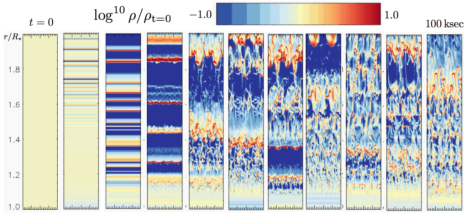
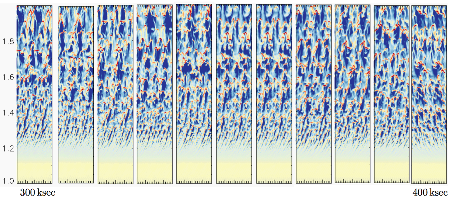
Figure 2: Spatial and temporal variations of log density relative to the initial, smooth ‘CAK’ steady-state at $t=0$, with color ranging from densities a decade below the $t=0$ value (blue) to a decade above (red). The vertical variation extends from the subsonic wind-base at the stellar surface $R_{\ast}$ to a height of one $R_{\ast}$ above. For clarity, the lateral variation is displayed over twice the horizontal box length $0.1R_{\ast}$. The upper row shows time evolution over the initial 100 ksec after the CAK initial condition, in steps of 10 ksec; the bottom row uses the same step-size of 10 ksec to show the evolution between 300 and 400 ksec, long after the initial condition has developed into a statistically steady turbulent flow.

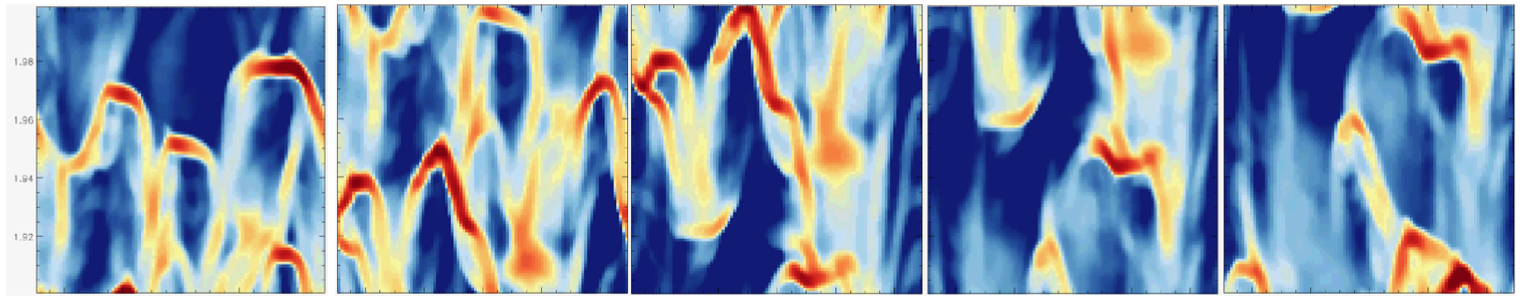
Figure 3: As in Fig. 2, spatial and temporal variations of log density relative to the initial, smooth ‘CAK’ steady-state at $t=0$ are shown, with color ranging from densities a decade below the $t=0$ value (blue) to a decade above (red). Here the vertical variation only extends between $1.9R_{\ast}$ and $2.0R_{\ast}$ and the lateral variation is displayed over one horizontal box of $0.1R_{\ast}$; there are thus $100\times 100$ discrete mesh-points in each of the displayed squares. From left to right are shown a 2 ksec time-evolution long after the initial condition, in steps of 0.5 ksec.

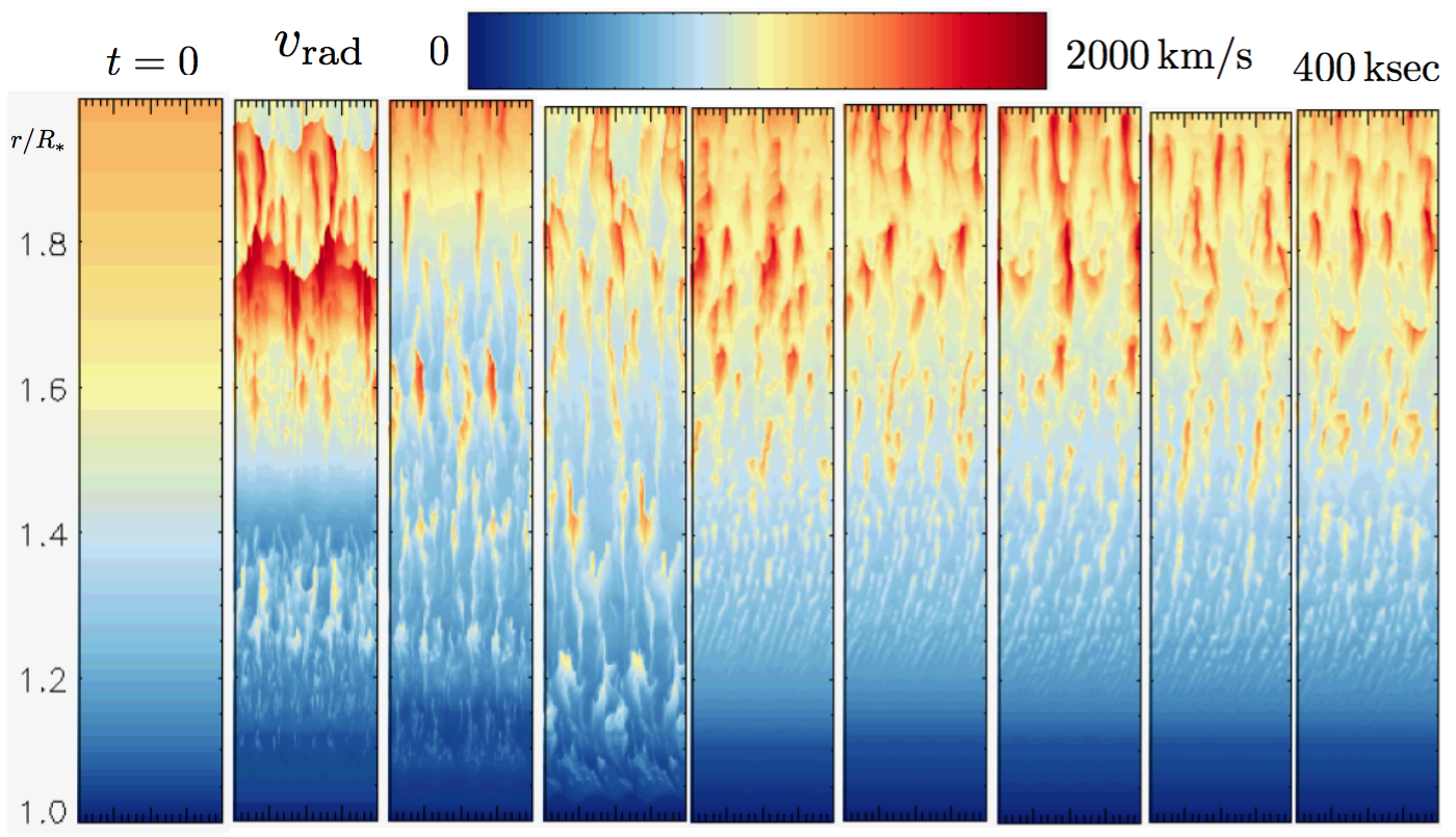
Figure 4: Spatial and temporal variations of radial velocity $\varv_{\rm rad}$, with color ranging from 0 (blue) to 2000 $\rm km/s$ (red). As in Fig. 2, the vertical variation extends from the subsonic wind-base at the stellar surface $R_{\ast}$ to a height of one $R_{\ast}$ above, and the lateral variation is displayed over twice the horizontal box length $0.1R_{\ast}$. The frames from left to right show the time evolution of $v_{\rm rad}$ over 400 ksec after the CAK initial condition, in steps of 50 ksec.

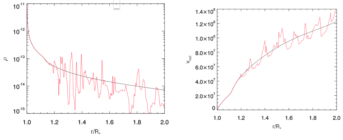
Figure 5: Radial cuts through the 2D simulation box of density $\rho\,\rm[g/cm^{3}]$ (left) and radial velocity $\varv_{\rm rad}\,\rm[cm/s]$ (right). The red curves are taken at a snapshot long after the simulation has developed into a statistically quite steady flow; the black curves compare this to average values.

Fig. 2 illustrates directly a key result of our simulations, namely the spatial and temporal variation in $\log\rho$ relative to the initial, smooth ‘CAK’ steady-state. The figure shows clearly how a radial shell structure first develops, but then quickly breaks up into laterally complex density variations. The upper panel displays snapshots during the first 100 $\rm ksec$ of the simulation, illustrating how already after a few dynamical flow-times $t_{\rm dyn}\approx R_{\ast}/\langle\varv_{\rm max}\rangle\approx\rm 11\,ksec$ the characteristic shells, seen in all 1D LDI simulations, brake up in what initially seem to resemble Rayleigh-Taylor structures. The lower panel then shows how, as time passes by, the structures eventually develop into a complex but statistically quite steady flow, characterized now by localized density enhancements (‘clumps’) of very small spatial scales embedded in larger regions of much lower density.

Fig. 3 zooms in on the same log density in a small $0.1R_{\ast}$ square-box over a short time-sequence long after the initial condition. This illustrates in greater detail the quite complex 2D density structure, showing a range of scales as well as high-density clumps with different shapes. The figure also demonstrates that, although the structures are small, they are clearly resolved by our numerical grid.

Fig. 4 displays temporal and spatial variations in radial velocity, illustrating essentially the same kind of outer-wind shock structure and high velocity streams as corresponding 1D simulations; however, also the velocity now exhibits extensive lateral variation, reflecting again the break-up of 1D shells into small-scale 2D clumps.

Fig. 5 emphasizes some similarities between these 2D simulations and corresponding 1D ones, by showing a radial cut through the simulation box at a time-snapshot (again taken long after the simulation has developed into a statistically steady flow). The figure demonstrates how such radial cuts indeed still show the characteristic structure of the non-linear growth of the LDI, namely high-speed rarefactions that steepen into strong shocks and wind plasma compressed into spatially narrow ‘clumps’ separated by rather large regions of rarified gas. There are some differences though: In addition to the lateral break-up of shells discussed above, another key distinction between 1D and 2D simulations is that the radial density variations are a bit lower in the latter; this occurs because of the lateral ‘filling in’ of radial rarefactions (see also Dessart & Owocki, 2003) and is discussed further in the following section.

3.1 Statistical properties

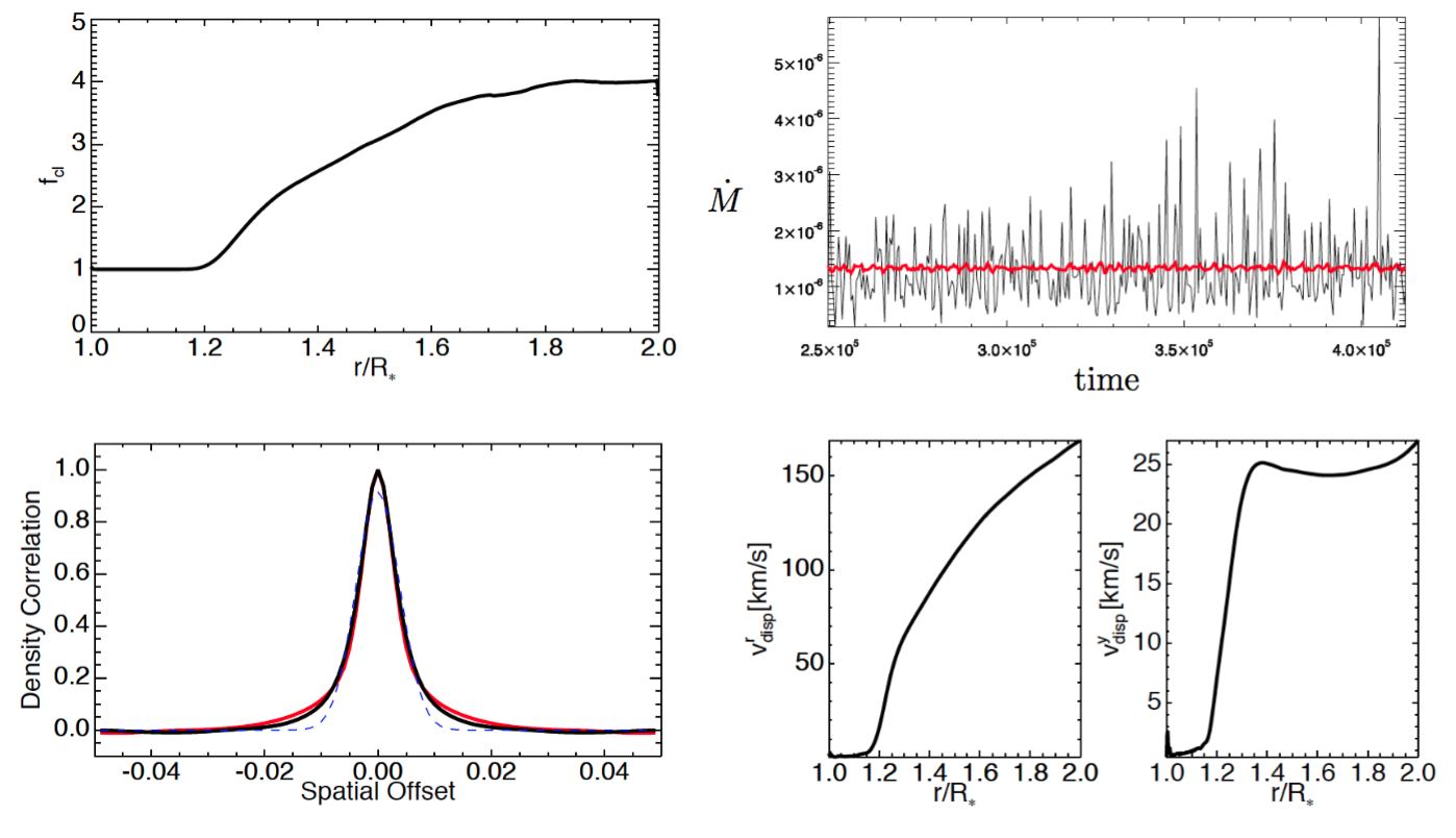
Figure 6: Selected statistical properties of the 2D simulation, see text. The upper left panel plots the clumping factor $f_{\rm cl}$; the upper right panel shows the time-dependent mass-loss rate, $\dot{M}\,\rm[M_{\odot}/yr]$ vs. sec., computed in two different ways for the red and black curves (see text); the lower left panel displays lateral (black) and radial (red) density correlation lengths as well as a Gaussian fit to these (blue, dashed); the lower right panel then finally plots radial (left) and lateral (right) velocity dispersions.

Fig. 6 summarizes some statistical results of the simulations. All averaging have here started at $t=250\,\rm ksec$, in order to separate out any dependence on the initial conditions and the adjustment to a new radiative force balance. The upper left panel in Fig. 6 shows the clumping factor:

$$f_{\rm cl}=\frac{\langle\rho^{2}\rangle}{\langle\rho\rangle^{2}},$$ (1)

where angle brackets denote averaging both laterally and over time in order to separate out $f_{\rm cl}$’s primary dependence on radius. The plot illustrates how the lateral ‘filling-in’ of radially compressed gas (see above) decreases the quantitative clumping factor significantly in a 2D simulation as compared to earlier 1D models where $f_{\rm cl}\ga 10$ (e.g., Sundqvist & Owocki, 2013); this is also consistent with the previous 2D results by Dessart & Owocki (2003). Note, however, that the actual values of $f_{\rm cl}$ in our 2D simulation are likely somewhat underestimated, due to our choice of stabilizing the wind-base against instability caused by nodal topology (see previous section). As discussed extensively by Sundqvist & Owocki (2013), in these near-photospheric layers the quantitative clumping factor is very sensitive to such choices made for the calculation of the radiative acceleration, as well as to any variability that may be assumed for the photospheric lower boundary. Regardless of such caveats, the basic qualitative result here that 2D simulations yield relatively lower values of $f_{\rm cl}$ than comparable 1D simulations is quite robust.

The upper right panel of Fig. 6 then shows the time-dependent mass-loss rate:

$$\dot{M}\equiv 4\pi r^{2}\rho\varv_{\rm rad}.$$ (2)

The black line in this plot shows a simple lateral average of the mass-flux escaping the outermost radial grid-point at a specific time. However, since our simulation box only covers $0.1R_{\ast}$, such an average very likely overestimates the time-dependent mass loss significantly. To compensate for this, the red curve in the plot instead uses an average over all grid-points $r\geq 1.5R_{\ast}$ at a specific time, which approximates averaging over a full stellar surface $4\pi(2R_{\ast})^{2}\approx 50R_{\ast}^{2}.$ As expected, this curve shows a drastically lower temporal variation of $\dot{M}$, despite the highly time-dependent flow. This is consistent e.g. with decade-long observations of spectral lines in O-stars, which typically indicate that time-variations in the mass-loss rate of such stars are low.

To estimate typical clump length-scales, the lower left panel of Fig. 6 plots a density autocorrelation length:

$$f_{\rm c}(\Delta)=\sum_{\rm time}\sum_{\rm i}(\rho_{i}-\langle\rho\rangle)\,(\rho_{i-\Delta}-\langle\rho\rangle),$$ (3)

where $\langle\rho\rangle$ averages laterally and over time. A lateral correlation length is calculated at each of the $\Delta=0-99$ lateral mesh-points and normalized to its $\Delta=0$ value. The figure then plots an average of this lateral correlation length between $r/R_{\ast}=1.9-2.0$ (black curve), as well as a radial correlation length (red curve) defined analogously. The lateral and radial density correlation lengths are very similar, and as such illustrates how a statistical ensemble of clumps is quite isotropic in these simulations. This does not imply that any given clump is isotropic (see Fig. 3), but rather that, on average, the well-developed density variations in the simulations do not have a strong preferred direction.

The Gaussian fit plotted in the blue dashed curve provides an estimate of the autocorrelation length in terms of the gaussian FWHM $\approx 0.01R_{\ast}$. Such small characteristic scales agree well with the theoretical expectation (see introduction) that the critical length scale for these clumpy wind simulations is of order the Sobolev length $\ell_{\rm Sob}$, which for the lateral direction at $2R_{\ast}$ is $\ell_{\rm Sob}/R_{\ast}=2\varv_{\rm th}/\varv\approx 0.01$. Identifying this as a typical clump length scale $\ell_{\rm cl}$, we may further make a simple estimate of the typical clump mass $\ell_{\rm cl}^{3}\rho_{\rm cl}\approx 10^{-6}R_{\ast}^{3}\,7\times 10^{-14}\,\rm g/cm^{3}\approx 10^{17}\,\rm g$, where the estimated clump density here simply reads off the output of the simulations (e.g., Fig. 5). More generally, such a clump mass-estimate may be obtained using the Sobolev length and mass conservation:

$$m_{\rm cl}\approx\ell_{\rm Sob}^{3}\rho_{\rm cl}\approx\frac{\varv_{\rm th}^{3}\dot{M}f_{\rm cl}r}{\varv^{4}4\pi},$$ (4)

which for the 2D simulation analyzed here indeed gives $m_{\rm cl}\approx 10^{17}\,\rm g$ for typical values at $2R_{\ast}$. Quite generally, eqn. 4 shows explicitly how rather low clump masses are expected to emerge from the LDI.

Finally, the lower right panels in Fig. 6 plots the radial and lateral velocity dispersions:

$$\varv_{\rm disp}=\sqrt{\langle\varv^{2}\rangle-\langle\varv\rangle^{2}},$$ (5)

where averages are constructed like for the clumping factor above. These plots show how, as expected (see also Dessart & Owocki 2003), the lateral velocity dispersion is on order the isothermal sound speed, whereas the radial dispersion is much higher and expected to rise above several hundreds $\rm km/s$ in the outer wind.

4 Summary and future work

We have introduced a pseudo-planar, box-in-a-wind approach suitable for carrying out radiation-hydrodynamical simulations in situations where the computation of the radiative acceleration is challenging and time-consuming. The method is used here to simulate the 2D non-linear evolution of the strong line-deshadowing instability (LDI) that causes clumping in the stellar winds from hot, massive stars. Accounting fully for both the direct and diffuse radiation components in the calculations of both the radial and lateral radiative accelerations, we examine in detail the small-scale clumpy wind structure resulting from our simulations.

Overall, the 2D simulations show that the LDI first manifests itself by mimicking the typical shell-structure seen in 1-D simulations, but these shells then quickly break up because of basic hydrodynamic instabilities like Rayleigh-Taylor and influence of the oblique radiation rays. This results in a quite complex 2D density and velocity structure, characterized by small-scale density ‘clumps’ embedded in larger regions of fast and rarefied gas.

While inspection of radial cuts through the 2D simulation box confirms that the typical radial structure of the LDI is intact, quantitatively the lateral ‘filling-in’ of gas leads to lower values of the clumping factor than for corresponding 1D models. A correlation-length analysis further shows that, statistically, density-variations in the well-developed wind are quite isotropic; identifying then the computed autocorrelation length with a typical clump size gives $\ell_{\rm cl}/R_{\ast}\sim 0.01$ at $2R_{\ast}$, and thus also quite low typical clump-masses $m_{\rm cl}\sim 10^{17}$ g. This agrees well with the theoretical expectation that the important length-scale for LDI-generated wind-structure is of order the Sobolev length $\ell_{\rm Sob}$.

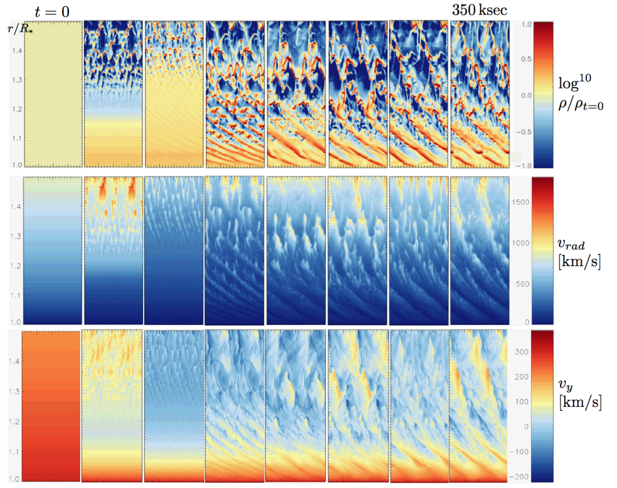
Figure 7: Spatial and temporal variations of log density, radial velocity, and lateral velocity for a model with stellar rotation at the surface $\varv_{\rm y}=300$ km/s (see text), with color ranging as in the earlier Figs. 2 and 4. The vertical variation in this simulation extends only from 1.0-1.5 $R_{\ast}$, but the lateral variation is displayed as before over twice the horizontal box length $0.1R_{\ast}$. From left to right are shown the time evolution over 350 ksec after the CAK initial condition, in steps of 50 ksec.

Influence of rotation and topology.

As noted in §2 and §3.1, the level of structure in near photospheric layers is likely underestimated in the simulation analyzed above, due to our choice to stabilize the wind base. To demonstrate this further, Fig. 7 shows a test-run with identical 2D set-up as before, but now introducing stellar rotation with a fixed $\varv_{\rm rot}=300$ km/s at the surface, and an initial condition set by steady-state angular momentum conservation, $\varv_{\rm y}(r)=\varv_{\rm rot}R_{\ast}/r$. The figure shows that once the simulation has adjusted to its new force conditions, radial streaks of high density now appear already at the surface; in other test-runs, we have found that such structures are typical for simulations with an unstable base and nodal topology. The radial streaks in this rotating model migrate along with the surface rotation, and embedded in the larger-scale structures are the typical small-scale clumps discussed previously. As speculated already in Sundqvist & Owocki (2015), these tentative first results thus suggest that rotating LDI models may quite naturally lead to the type of combined large- and small-scale structure needed to explain in parallel various observed phenomena in hot-star winds, like discrete absorption components (DACs) (Kaper et al., 1999) and small-scale wind clumping (Eversberg et al., 1998). Future work will examine in detail connections between these rotating LDI models and the presence of various types of wind sub-structure.

The simulations presented in this paper also lead naturally to a number of follow-up investigations; already in the pipe-line are the development of a formalism for characterizing porosity-effects in turbulent media (Owocki & Sundqvist 2017) and the influence of the clumpy wind on the accretion properties of an orbiting neutron star in a so-called high-mass X-ray binary (HMXB) system (el-Mellah et al. 2017). More directly related to this paper, we also plan to (in addition to further analyzing the effects of rotation and topology) extend the current simulations to 3D and to higher wind radii, and also develop a more general radiative transfer scheme (allowing for an arbitrary number of rays) for the computation of the line acceleration within a pseudo-planar box-in-a-wind.

Appendix A 2D pseudo-planar line-force

Our development here of a 2D vector form for the line-acceleration follows a direct generalization of the 1D SSF method detailed in Owocki and Puls (1996; hereafter OP96), as further developed in Sundqvist and Owocki (2015, hereafter SO15). As discussed in OP96 (cf. their equation (3)), a key step is to compute efficiently the profile-weighted line optical depth between two wind locations along some ray coordinate $z$,

$$\Delta t(x,z_{1},z_{2})=\int_{z_{1}}^{z_{2}}\kappa_{\rm o}\rho(z)\phi[x-u_{z}(z)]\,dz\,,$$ (6)

where $\kappa_{\rm o}$ is a spatially constant line opacity normalization, and $u_{\rm z}\equiv\bf{\hat{z}}\cdot\bf{u}$ is the local $z$-projection of the vector flow velocity normalized to the ion thermal speed, ${\bf u}\equiv{\bf\varv}/v_{\rm th}$. The line-profile function is taken here to have a normalized gaussian form, $\phi(x)=e^{-x^{2}}/\sqrt{\pi}$, with $x=(\nu-\nu_{\rm o})/\Delta\nu_{\rm D}$ the observer-frame frequency displacement from line-center in thermal doppler units $\Delta\nu_{\rm D}=\nu_{\rm o}v_{\rm th}/c$.

In 1D spherically symmetric models in which variables only depend on the radius $r$, the ray direction is defined in terms of the local $r$ and a stellar impact parameter $p$, with $|z|=\sqrt{r^{2}-p^{2}}$, and the sign taken to be positive (negative) in the forward (backward) hemisphere. Moreover, since the velocity is purely radial ${\bf u}=u_{\rm r}\bf{\hat{r}}$, we have simply $u_{\rm z}=\mu_{\rm z}u_{\rm r}$, with radial projection cosine $\mu_{\rm z}=z/r$.

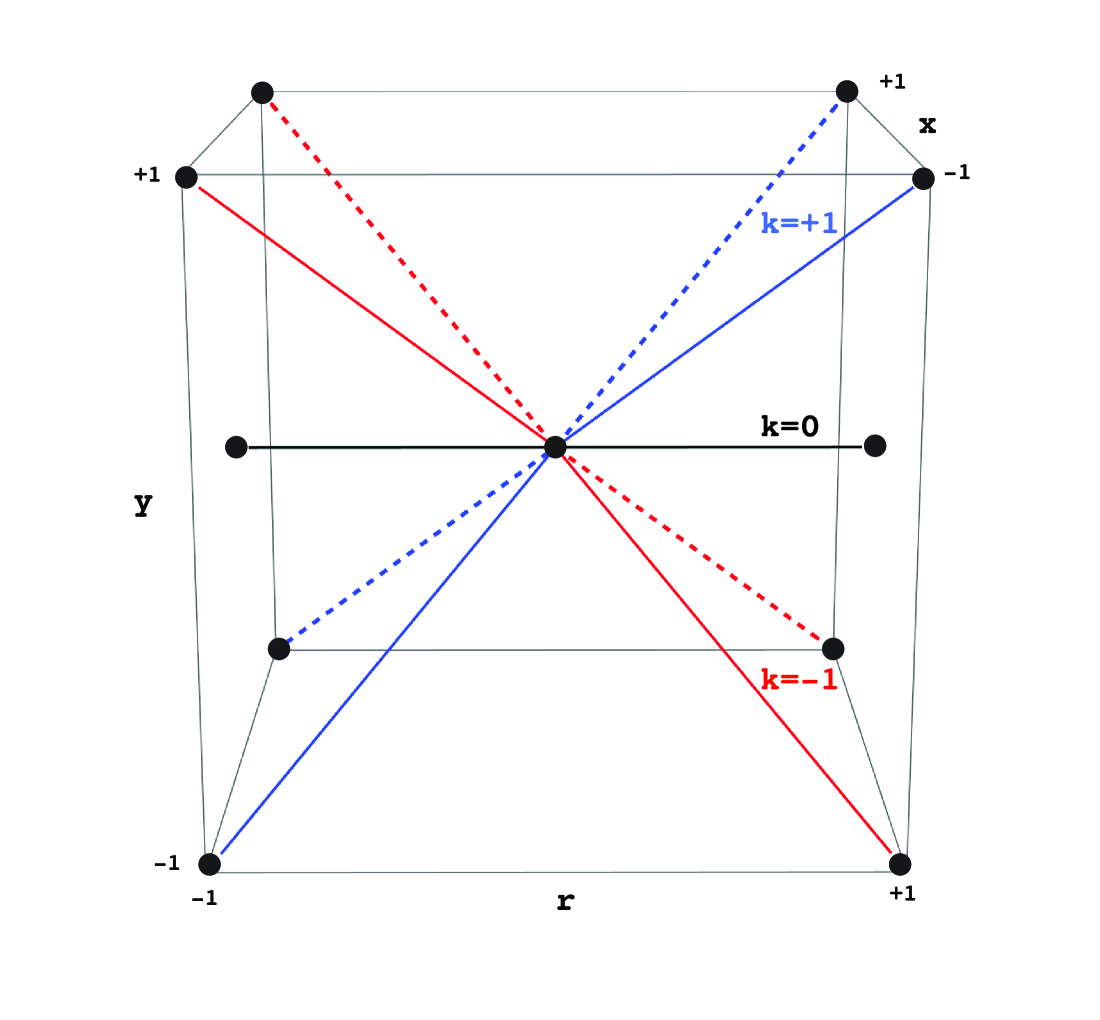
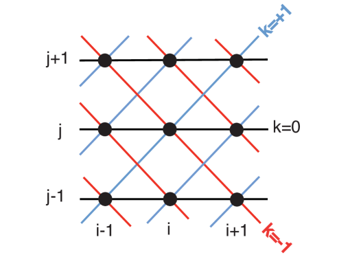
Figure 8: Illustration of ray trajectories in the prograde ($k=+1$; blue), radial ($k=0$; black), and retrograde ($k=-1$; red) directions, crossing grid nodes (black dots) that neighbor a central node with spatial indices $\{i,j\}$. The upper panel shows the full 3D geometry of the radiation rays. But since conditions are assumed constant in x (and thus symmetric about x=0), ray integrations computed along dashed and solid lines of the same color are identical, and so can be accounted for by simply doing one prograde (blue) and one retrograde (red) integration, and then giving these double weight in the angle quadrature. The lower panel shows these final 3 distinct rays projected upon the 2D $r-y$ calculation plane.

In the present 2D pseudo-planar formulation, variations can occur in both radius $r$ and a lateral orthogonal direction $y$, taken to lie in the equatorial plane of symmetry. The ray directions $z$ now have local projection cosines $\mu_{\rm r}$ and $\mu_{\rm y}$ relative to the $r$ and $y$ axes, with thus $u_{\rm z}=\mu_{\rm r}u_{\rm r}+\mu_{\rm y}u_{\rm y}=\mu u_{\rm r}+\sin\phi\sqrt{1-\mu^{2}}u_{\rm y}$, with $\theta\equiv\arccos{\mu}$ and $\phi$ the customary radiation angles in §2. Our computations include one purely radial ray, with $\mu_{\rm r}=1$ and $\mu_{\rm y}=0$, so that $u_{\rm z}=u_{\rm r}(r,y)$; as noted in §2, we also formally account for four additional rays that all have $\mu_{\rm r}=1/\sqrt{3}$, with two pairs of rays with $\mu_{\rm y}=\pm 1/\sqrt{3}$, but each pair forming mirror projections above/below the $r-y$ plane. In practice, because of the mirror symmetry about this plane, explicit computation is only needed for one pair, with the other pair simply accounted for by doubling the quadrature weights (see Fig. A1). For notational convenience, let us denote this triad with an index $k=-1,0,1$, such that $\mu_{{\rm r},0}=1$ and $\mu_{{\rm r},\pm 1}=1/\sqrt{3}$, while $\mu_{{\rm y},0}=0$ and $\mu_{{\rm y},\pm 1}=\pm 1/\sqrt{3}$ (see Fig. 8).

For our uniform spatial grid with fixed spacings $\Delta r=\Delta y=\Delta=0.001R_{\ast}$, we have coordinates $r_{\rm i}=R_{\ast}+i\Delta$ and $y_{\rm j}=j\Delta$, for grid indices $i=$1 to $n_{\rm r}=1000$ and $j=$1 to $n_{\rm y}=100$. At each grid node $\{i,j\}$, the outward (+) increment in optical depth $\Delta t_{\rm+,ijk}(x)$ along each of the directional triad $k$ is computed from (6), assuming a piecewise linear variation of density $\rho$ and velocities $u_{\rm r}$ and $u_{\rm y}$ to the next outer grid node, with indices $\{i+1,j+k\}$. Summation from the lower boundary at the stellar surface then gives the associated outwardly integrated optical depths along each direction $k$ to some node with coordinates $\{r,y\}$,

$$t_{\rm+,k}(x,r,y)=\sum_{\rm i,j}\Delta t_{\rm+,ijk}(x)+t_{\rm+,k}(x,R_{\ast},y_{\ast})\,,$$ (7)

where the summation is understood to be over all $i$ below the index for $r$, and over the associated $j$ variation for each particular ray $k$; the assumed periodic variation in $y$ means that $j$ indices are simply mapped onto the range $0<j<100$ by taking ${\rm mod}(j,100)$. This means that all rays considered here in the pseudo-planar model hit the stellar surface at the lower boundary of the grid. The surface boundary value allows one to account for a photospheric line-profile and the effect of a cutoff at a maximum opacity $\kappa_{\rm max}$ in the line distribution, as given by equation (OP96-66),

$$t_{\rm+,k}(x,R_{\ast},y_{\ast})=\frac{\kappa_{\rm o}}{\kappa_{\rm max}}+\frac{\kappa_{\rm o}\phi(x)}{\kappa_{\rm e}}\,.$$ (8)

With the outward optical depths $t_{\rm+,k}(x,r,y)$ in hand, the computation of the resulting radial component of the line-acceleration follows much the same approach as for the 1D SSF formalism given in section 5.3 of OP96, as further elaborated in section 2.1 of SO15. The direct absorption component of gravitationally scaled line-acceleration thus takes the form (cf. (SO15-3))

$$\Gamma_{\rm dir,r}(r,y)=\Gamma_{\rm thin}\sum_{x,k}w_{\rm x}w_{\rm k}\,\phi\left(x-u_{\rm z,k}\right)t_{\rm+,k}^{-\alpha}(x,r,y)\,,$$ (9)

where $u_{\rm z,k}\equiv\mu_{\rm r,k}u_{\rm r}(r,y)+\mu_{\rm y,k}u_{\rm y}(r,y)$, and the optically thin normalization $\Gamma_{\rm thin}$ is given by (SO15-4). As in 1D models, the quadrature in frequency $x$ is uniform with equal weights $w_{\rm x}=\Gamma(\alpha)/n_{\rm x}$, and a resolution of three points per thermal doppler width, $\Delta x=1/3$; but the 1D angle-quadrature weight $w_{\rm y}$ is now replaced with the triad $w_{\rm k}$, with normalized values $w_{0}=0.211325$ and and $w_{\pm 1}=0.394338$. This triad weights the oblique rays such that they cover the full $\mu$-space from 0 to $1/\sqrt{3}$, plus half the space from $1/\sqrt{3}$ to a radial ray at $1$; the radial ray thus get the weight $w_{0}=(1-1/\sqrt{3})/2=0.211235$.

Within this SSF formalism, the diffuse (scattering) component of the line-force is again (see OP96) formed by using $t_{+}$ to build an associated inward optical depth $t_{-}$, and using this to form a difference between the outward vs. inward escape probability, as given in equation (SO15-6). To avoid the variability of a nodal topology at the wind base (see §3 of SO15), we assume a simple optically thin source function computed from a uniformly bright surface without limb darkening, as given in equation (SO15-8).

Our computation of the lateral ($y$) component of the line-force warrants some further elaboration. While the overall formulation is similar, this now depends the difference between the escape probabilities in prograde ($k=+1$) and retrograde ($k=-1$) directions, applied to both the direct and diffuse components. (The radial ray $k=0$ plays no role.) Defining the profile-averaged, outward (+) escape probabilities in the prograde/retrograde ($\pm$) directions as

$$b_{+,\pm}(r,y)=\sum_{x}w_{x}\,\phi\left(x-u_{z,\pm 1})\right)t_{+,\pm 1}^{-\alpha}(x,r,y)\,,$$ (10)

we can write the direct component of the lateral line-acceleration (still scaled by the radial gravity) as

$$\Gamma_{\rm dir,y}(r,y)=\Gamma_{\rm thin}f(r)\left[b_{+,+}(r,y)-b_{+,-}(r,y)\right]\,.$$ (11)

To account for the additional radial drop-off associated with angular shrinking of the stellar core (e.g., Gayley & Owocki 2000), we include here a correction factor

$$f(r)=w_{1}\mu_{\rm y,+1}\,\frac{R_{\ast}^{2}}{r^{2}}\,.$$ (12)

Defining inward (–) escape probabilities in a way analogous to (10), we can write the associated diffuse component of the lateral line-acceleration as

$$\Gamma_{\rm diff,y}(r,y)=\Gamma_{\rm thin}\,s(r)\left[b_{-,+}+b_{+,-}-b_{+,+}-b_{-,-}\right]\,,$$ (13)

where the optically thin source function factor $s(r)$ is given by equation (SO15-8). For both the radial ($r$) and lateral ($y$) components, the associated total acceleration is given by the sum of the direct and diffuse contributions, $\Gamma_{\rm tot}=\Gamma_{\rm dir}+\Gamma_{\rm diff}$.

In our numerical radiation-hydrodynamics simulations, we apply these total radial and lateral line-accelerations in the associated radial and lateral momentum equations,

$$\frac{\partial\varv_{r}}{\partial t}+\varv_{r}\frac{\partial\varv_{r}}{\partial r}=-\frac{1}{\rho}\frac{dP}{dr} + (\Gamma_{\rm tot,r}-1)\frac{GM_{\rm eff}}{r^{2}}+\frac{\varv_{\rm y}^{2}}{r}\,$$ (14)

$$\frac{\partial\varv_{y}}{\partial t}+\varv_{y}\frac{\partial\varv_{y}}{\partial r}=-\frac{1}{\rho}\frac{dP}{dy} + \Gamma_{\rm tot,y}\frac{GM_{\rm eff}}{r^{2}}-\frac{\varv_{\rm r}\varv_{\rm y}}{r}\,,$$ (15)

where $P$ is the gas pressure, $M_{\rm eff}\equiv M(1-\Gamma_{\rm e})$, and the last term in each equation corrects our pseudo-planar treatment for curvilinear coordinate effects (‘centrifugal’ and ‘coriolis’ forces) in a spherical outflow. The density $\rho$ is evolved according to the mass continuity equation,

$$\frac{\partial\rho}{\partial t}+\frac{\partial(\rho\varv_{r})}{\partial r}+\frac{\partial(\rho\varv_{y})}{\partial y}=-\frac{2\rho\varv_{r}}{r}\,,$$ (16)

where the source term on the right-hand-side corrects for the neglect of the spherical divergence within our pseudo-planar treatment of the flow divergence $\nabla\cdot(\rho{\bf\varv})$. The $1/r^{2}$ decline of the radiative flux, which sets the scale of the line-accelerations, is accounted for by scaling these accelerations with the inverse-square decline of the stellar gravity.