A Tight Excess Risk Bound via a Unified PAC-Bayesian–Rademacher–Shtarkov–MDL Complexity
Abstract
We present a novel notion of complexity that interpolates between and generalizes some classic existing complexity notions in learning theory: for estimators like empirical risk minimization (ERM) with arbitrary bounded losses, it is upper bounded in terms of data-independent Rademacher complexity; for generalized Bayesian estimators, it is upper bounded by the data-dependent information complexity (also known as stochastic or PAC-Bayesian, complexity. For (penalized) ERM, the new complexity reduces to (generalized) normalized maximum likelihood (NML) complexity, i.e. a minimax log-loss individual-sequence regret. Our first main result bounds excess risk in terms of the new complexity. Our second main result links the new complexity via Rademacher complexity to entropy, thereby generalizing earlier results of Opper, Haussler, Lugosi, and Cesa-Bianchi who did the log-loss case with . Together, these results recover optimal bounds for VC- and large (polynomial entropy) classes, replacing localized Rademacher complexity by a simpler analysis which almost completely separates the two aspects that determine the achievable rates: ‘easiness’ (Bernstein) conditions and model complexity.
1 Introduction
We simultaneously address four questions of learning theory:
-
(A)
We establish a precise relation between Rademacher complexities for arbitrary bounded losses and the minimax cumulative log-loss regret, also known as the Shtarkov integral and normalized maximum likelihood (NML) complexity.
-
(B)
We bound this minimax regret in terms of entropy. Past results were based on entropy.
-
(C)
We introduce a new type of complexity that enables a unification of data-dependent PAC-Bayesian and empirical-process-type excess risk bounds into a single clean bound; this bound recovers minimax optimal rates for large classes under Bernstein ‘easiness’ conditions.
-
(D)
We extend the link between excess risk bounds for arbitrary losses and codelengths of Bayesian codes to general codes.
All four results are part of the chain of bounds in Figure 1. The arrow stands for ‘bounded in terms of’; the precise bounds (which may hold in probability and expectation or may even be an equality) are given in the respective results in the paper. Red arrows indicate results that are new.
l59.5ptt31pt\makebox(37.0,7.0)[]{}\stackinsetl59.5ptt41pt\makebox(30.0,5.0)[]{}\stackinsetl174ptt32.5pt\makebox(35.0,5.5)[]{}\stackinsetl331ptt16pt\makebox(43.5,6.5)[]{}\stackinsetl252.5ptt124.5pt\makebox(39.0,5.0)[]{}\stackinsetl252.5ptt133.5pt\makebox(40.0,6.5)[]{}\stackinsetl252.5ptt182.5pt\makebox(39.0,5.0)[]{}\stackinsetl252.5ptt191.5pt\makebox(40.0,6.5)[]{}\stackinsetl316ptt165.5pt\makebox(38.5,5.5)[]{}\stackinsetl301ptt220pt\makebox(39.0,5.5)[]{}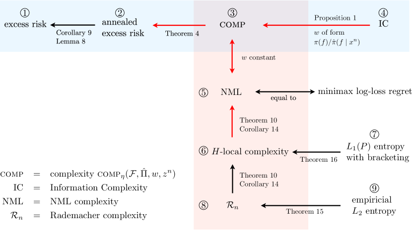
We start with a family of predictors for an arbitrary loss function , which, for example, may be log-loss, squared error loss or -loss, and an estimator which on each sample outputs a distribution on ; classic deterministic estimators such as ERM are represented by taking a that outputs the Dirac measure on . The main bound , Theorem 4, bounds the annealed excess risk of a fixed but arbitrary estimator in terms of its empirical risk on the training data plus a novel notion of complexity, (formulas for and all other concepts in the paper are summarized in the Glossary on page 6). The annealed excess risk is a proxy (and lower bound) of the actual excess risk, the expected loss difference between predicting with and predicting with the actual risk minimizer within . The bound (Corollary 9, based on Lemma 8, itself from Grünwald (2012)) bounds the actual excess risk in terms of the annealed excess risk, so that we get a true excess risk bound for . The complexity is dependent on a luckiness function ; can be chosen freely; different choices lead to different complexities and excess risk bounds. For nonconstant , the complexity becomes data-dependent; in particular, for of the form , where is the density of a ‘prior’ distribution on , the complexity becomes, by (Proposition 1) (strictly) upper bounded by the information complexity of Zhang (2006a, b), involving a Kullback-Leibler (KL) divergence term . Information complexity generalizes earlier complexity notions and accompanying bounds from the information theory literature such as (extended) stochastic complexity (Rissanen, 1989; Yamanishi, 1998), resolvability (Barron and Cover, 1991; Barron et al., 1998), and also excess risk bounds from the PAC-Bayesian literature (Audibert, 2004; Catoni, 2007). Together, recover and strengthen Zhang’s bounds.
For constant , the complexity is independent of the data and turns out (), Section 2.2) to be equal to the minimax cumulative individual sequence regret for sequential prediction with log-loss relative to a family of probability measures defined in terms of , also known as the log-Shtarkov integral or NML (Normalized Maximum Likelihood) complexity. NML complexity has been much studied in the MDL (minimum description length) literature (Rissanen, 1996; Grünwald, 2007).
Problem A: NML and Rademacher
NML complexity can itself be bounded in terms of a new complexity we introduce, -local complexity, which is further bounded in terms of Rademacher complexity (Theorem 10 and Corollary 14, ). Both Rademacher and NML complexities are used as penalties in model selection (albeit with different motivations), and the close conceptual similarity between NML and Rademacher complexity has been noted by several authors (e.g. Grünwald (2007); Zhu et al. (2009); Roos (2016)). For example, as shown by Grünwald (2007, Open Problem 19, page 583) in classification problems, both the empirical Rademacher complexity for 0-1 loss and the NML complexity of a family of conditional distributions can be simply expressed in terms of a (possibly transformed) minimized cumulative loss that is uniformly averaged over all possible values of the data to be predicted, thereby measuring how well the model can fit random noise. Theorem 10 and Corollary 14 establish, for the first time, a precise and tight link between NML and Rademacher complexity. The proofs extend a technique due to Opper and Haussler (1999), who bound NML complexity in terms of entropy using an empirical process result of Yurinskiĭ (1976). By using Talagrand’s inequality instead, we get a bound in terms of Rademacher complexity.
Problem B: Bounding NML Complexity with entropy and empirical Entropy
If is of VC-type or a class of polynomial empirical entropy, the Rademacher complexity can be further bounded, (Theorem 15, ), in terms of the empirical entropy; if admits polynomial entropy with bracketing, then is further bounded, (Theorem 16, ), in terms of this entropy with bracketing. These latter two results are well-known, due to Koltchinskii (2011) and Massart and Nédélec (2006) respectively, but in conjunction with they become of significant interest for log-loss individual sequence prediction. Whereas previous bounds on minimax log-loss regret were invariably in terms of entropy (Opper and Haussler, 1999; Cesa-Bianchi and Lugosi, 2001; Rakhlin and Sridharan, 2015), the aforementiond two results allow us to obtain bounds in terms of entropy and empirical entropy, where can be any member of the class . Unlike the latter two works, however, our results are restricted to static experts that treat the data as i.i.d.
Problem C: Unifying data-dependent and empirical process-type excess risk bounds
As lamented by Audibert (2004; 2009), despite their considerable appeal, standard PAC-Bayesian and KL excess risk bounds do not lead to the right rates for large classes, i.e. with polynomial entropy. On the other hand, standard Rademacher complexity generalization and excess risk bound analyses are not easily extendable to either penalized estimators or generalized Bayesian estimators that are based on updating a prior distribution; also handling logarithmic loss appears difficult. Yet shows that there does exist a single bound capturing all these applications — by varying the function one can get both (a strict strengthening of) the KL bounds and a Rademacher complexity-type excess risk bound. In this way, via the chain of bounds , we recover rates for empirical risk minimization (ERM) that either are minimax optimal (for classification) or the best known rates for ERM (for other losses), even for VC and polynomial entropy classes; the rates depend in the right way on the ‘easiness’ of the problem as measured by the central condition (van Erven et al., 2015), which generalizes Tsybakov’s (2004) margin condition and Bernstein conditions (Bartlett et al., 2005).
Problem D: Excess Risk Bounds and Data Compression
While Zhang’s bound holds for arbitrary ‘posteriors’ , one gets the best excess risk bounds if one takes to be a generalized Bayesian estimator. With such a , the information complexity can be expressed in terms of a (generalization of) the cumulative log-loss of a Bayesian sequential prediction strategy (Zhang, 2006a; Grünwald, 2012) defined relative to the constructed probability model . By the correspondence between codelengths and cumulative log-loss (reviewed in Section 2), we may say that we bound an excess risk in terms of a codelength. shows that we also get a useful excess risk bound in terms of the codelengths of the minimax (NML) code — interestingly, Bayes and NML codes are the two central codes in the universal coding literature (Barron et al., 1998; Grünwald, 2007). In fact, our work shows that the correspondence between excess risk bounds and codelengths is a quite general phenomenon, not particular to Bayes and NML codes: in Section 2 we show that there is a 1-to-1 relation between luckiness functions and codes for data based on : each luckiness function defines, up to scaling, a different code giving rise to a different complexity and hence a different excess risk bound, and vice versa. Because of its relation to data compression, it becomes easy to extend the approach to model selection by using ‘two-part codes’ (Section 5.1).
For yet other choices of , we obtain bounds for penalized ERM with arbitrary bounded penalization functions (Section 5.2); if we specialize to log-loss, the complexity bound becomes a minimax regret-with-luckiness-term as considered in recent papers on sequential log-loss prediction such as (Kakade et al., 2006; Bartlett et al., 2013). Many other choices of are possible and remain subject for future investigation.
Additional Features and Limitations
The full story above can only be told for bounded losses, although the bounds also hold for unbounded losses, and was recently extended to unbounded losses under a mild additional condition (Grünwald and Mehta, 2016). Remarkably, is as tight as can be: when viewed in terms of exponential moments, it is really an equality rather than a bound; this suggests that, no matter the choice of , the resulting bound is essentially unimprovable. The complexity depends on a learning rate parameter , and all bounds in the figure become different depending on the choice of . The optimal depends on the easiness of the problem at hand, as measured by central/Bernstein/Tsybakov’s conditions (see above). ERM can be applied (and optimal rates can be obtained) without knowledge of the optimal ; to get the right rates for Bayesian and penalized ERM algorithms however, these algorithms should be made dependent on ( is akin to in the lasso and ridge regression); in practice, one can learn it from the data using an algorithm such as the ‘safe Bayes’ algorithm of Grünwald (2012) (Section 5.1).
Contents
In Section 2.2, we introduce the simple data-independent version of our complexity, , which is really the NML complexity. In Section 2.4 we extend our notion of complexity to the generalized data-dependent form . Section 3 contains our first main result, Theorem 4. In Section 4, we derive our second main result, Theorem 10 and its Corollary 14, a bound on in terms of Rademacher complexity; we also present a concrete application of this result, Theorem 20, which provides the best known rates for ERM under Bernstein conditions for bounded loss functions in a number of situations. Section 5 gives various applications of our result. Finally, Section 6 closes with a discussion of our work in the context of other recent works. All long proofs can be found in the appendix. Mathematical definitions and notations are summarized in the Glossary on page 6.
2 The Novel Complexity Notion
2.1 Preliminaries
In the statistical learning problem (Vapnik, 1998), a labeled sample is drawn independently from probability distribution over , where, for each , we have . We are given an action space or model and a loss function , where we denote the loss that action or predictor makes on as . Loss functions such as 0-1, squared error, and log-loss (for joint densities on ) can all be expressed this way: in the former two cases consists of functions , with and respectively, and in the latter case is a set of probability densities on relative to some underlying measure and , with denoting natural logarithm in this paper. An estimator or learning algorithm is a function from to distributions over . Here and in the sequel we simply assume that is endowed with a suitable sigma-algebra so that is a measurable space and all functions we refer to are measurable. We will write to denote the distribution chosen for data . In practice is often supported entirely on a single function ; in that case we simply write the estimator as and the chosen for given data as . An example of such a deterministic estimator is ERM, the empirical risk minimizer. An example of a randomized estimator is obtained by setting to be the generalized -Bayesian posterior (Zhang, 2006b; Catoni, 2007), which we explicitly define in Section 2.4. Henceforth, we simply call an ‘estimator’ irrespective of whether it is deterministic or randomized.
We aim to learn distributions that obtain low expected risk . The risk of an action is the expected value of the loss suffered when playing action and the actual outcome is . A natural way to measure the quality of on data is therefore the excess risk , where is a minimizer of the risk over ; like many other authors (e.g Bartlett et al. (2005)) we assume throughout this work that such a minimizer exists. We use the notation , extended to samples as . Note that, when , and can be thought of as random variables so we simply write them without whenever this cannot cause any confusion.
2.2 The Novel Complexity Measure, Simple Case
To prepare for the definition of our complexity measure comp, we first need to associate each with an associated probability distribution . We may assume without loss of generality that the underlying distribution on has a density with respect to some base measure (we could for example take but the formulas below are easier to parse for general ). Now for each , we define to be the distribution over with density (with respect to the same base measure )
| (1) |
We extend the definition to outcomes by taking the product densities, . In this way the model is itself mapped to a set of probability densities, the mapping depending on the loss function of interest, but also (suppressed in notation) on , , and on the ‘true’ ; this is an instance of the ‘entropification procedure’ suggested by Grünwald (1999).
We are now ready to define our new complexity measure. For simplicity of we first present the very special case of deterministic estimators without data dependence; this case is sufficient to make the connection to minimax regret and Rademacher complexities in Section 4. For this setting we define the Shtarkov integral (name to be explained below) as
| (2) |
where, for any , is the normalization constant. Whenever is finite (as will automatically be the case with bounded loss), the corresponding complexity of model equipped with is defined as
| (3) |
, and normalizer all depend on , but this is suppressed in notation unless needed for clarity. The final equality in (2) holds in the very special case that the original loss function is log-loss, , and contains the density of (‘the model is correct’). In that case (since log-loss is a proper loss, see e.g. (Gneiting and Raftery, 2007)) evaluates to for all , is equal to , and ; thus, (1) reduces to , and the final equation in (2) follows. We further define the maximal complexity as
| (4) |
where the final equality is a trivial consequence of the definition, the ranging over all deterministic estimators that can be defined on .
We often use the following observation due to (e.g.) Opper and Haussler (1999): Let be a finite set and let be a partition of . Then for every deterministic estimator,
| (5) |
This result follows as a special case of Proposition 22 in Section 5, but its proof is simple enough to state in just a few lines:
Using (5), we can link comp to Rademacher complexity, which we will do in Section 4.1 and 4.2. Below, we first link comp to log-loss prediction, extend it to encompass data-dependent and PAC-Bayesian complexities and present our excess risk bound for the general complexities (Section 4.1 and 4.2) can be read without this material).
Minimax Cumulative Log-Loss Interpretation of comp
For every given estimator , we can define a density on relative to by setting
| (6) |
which evidently integrates to and hence is a probability density (different choice of estimator leads to different ; this is suppressed in the notation). We can use density to sequentially predict by predicting with the corresponding conditional density . The cumulative log-loss obtained this way is given by
the latter equality following by definition of conditional probability and telescoping. Because of the correspondence, via Kraft’s inequality, of log-loss prediction and data compression, we can also think of this quantity as a codelength. Similarly, is the minimum cumulative loss one could have obtained with hindsight, i.e. if one had sequentially predicted the by the that turned out to minimize on . Assuming this minimum is well-defined it is of course achieved by , the maximum likelihood estimator relative to , for which evidently also . Thus we get that for all ,
| (7) |
the first equation holding for general and the second for . The final expression is just the (cumulative log-loss) regret of on data , which, by (2.2), is constant on . As first noted by Shtarkov (1987), this implies that (2.2) is also the minimax individual-sequence regret relative to the model when sequentially predicting outcomes with the log-loss; the corresponding optimal sequential prediction strategy is usually called the normalized maximum likelihood (NML) or Shtarkov density; see Rissanen (1996); Grünwald (2007); Opper and Haussler (1999); Cesa-Bianchi and Lugosi (2001) for details.
2.3 Allowing Data-Dependency
We now generalize the complexity definition above for arbitrary deterministic so that it becomes data dependent; further extension to randomized estimators follows in Section 2.4. The central concept we need is that of a luckiness function ; every combination of estimator and luckiness function will, up to scaling, define a unique version of complexity; and every such complexity will induce a different data-dependent bound on excess risk. We call ‘luckiness function’ since it will influence our excess risk bounds so that they become better iff we are ‘lucky’ in the sense that is such that will be large with high probability).
The generalized Shtarkov integral for estimator relative to luckiness function is defined as
| (8) |
and, whenever , we define the corresponding data-dependent complexity as
| (9) |
Both expressions evidently reduce to (2) and (3) if we take constant over .
Cumulative Log-Loss Interpretation
Fix an arbitrary estimator . Then for any luckiness function with , we can define the probability density
| (10) |
with (6) being the special case with . Just as with , for general such , can be thought of as a sequential prediction strategy, and is the cumulative log-loss achieved by . Different (up to scaling) generate different log-loss prediction strategies (codes) and corresponding complexities. Conversely, for every probability density relative to on , we can set a luckiness measure proportional to ; with the appropriately scaled choice of , will coincide ; we thus have a -to--correspondence between luckiness functions with , codes and complexities.
2.4 The Novel Complexity Measure, General Case
Here we further generalize the complexity definition so that it can output distributions on . For this we need to extend the domain of the luckiness function to encompass , i.e. we now take arbitrary functions of the form .
The generalized Shtarkov integral for estimator relative to luckiness function is defined as
| (11) |
and the generalized (data-dependent) model complexity corresponding to (11) is now defined as
| (12) |
Both expressions are readily seen to generalize (8) and (9) respectively: if, for a given deterministic estimator , we take to be (the Dirac measure on ) and we take a function that does not depend on , then the expressions above simplify trivially to (8) and (9) respectively; thus . Finally, we define
| (13) |
as the sum of the complexity and the expected excess loss that a random draw from achieves on the data.
comp generalizes information complexities
To explain how PAC-Bayesian type complexity arise a special case of comp, we consider luckiness measures that are defined in terms of probability distributions on that do not depend on the data; we call these ‘priors’. For notational convenience it is useful to assume (without loss of generality) that has a density relative to some underlying measure on and that, for all , also has a density relative to .
Proposition 1
Consider arbitrary and as above with densities and relative to some . Set . Then we have
| (14) |
Consequently,
| (15) |
where is KL divergence.
Proof By Jensen’s inequality applied to (11), we have, using the definition of and Fubini’s theorem,
which gives (14); (15) follows by plugging in our choice of into the definition of comp.
We thus see that is upper bounded by information complexity defined relative to prior (Zhang, 2006a, b), which is just (15) normalized (divided by ). The notion of information complexity is also used to bound excess risks in the PAC-Bayesian approach of Catoni (2007) and Audibert (2004). As noted by Zhang (2006b), the right-hand side of (15) is minimized if we take as our estimator the -generalized Bayesian estimator,
| (16) |
and in that case is equal to the generalized marginal likelihood, known in the MDL literature as the extended stochastic complexity (Yamanishi, 1998)
| (17) |
which, for and the log-loss, coincides with the standard log Bayesian marginal likelihood.
We provide some further simple properties of for general and in Section 5.
Cumulative Log-Loss Interpretation
Just as for deterministic estimators, we note that every randomized estimator and luckiness function defines a probability density/prediction strategy on by setting
and just as before, comp can be interpreted in terms of the ‘code’ .
3 First Main Result: Bounding Excess Risk in Terms of New Complexity
In this section and Section 4, we restrict to the bounded loss setting; given this restriction, it is without loss of generality that we assume that
| (A1) |
as this always can be accomplished by an appropriate scaling of the loss.
Before presenting our first main result, it will be useful to introduce a variant of an ordinary expectation as well as some notation. For and general random variables , we define the annealed expectation (see Grünwald and Mehta (2016) for the origin of this terminology) as
| (18) |
Below we will first bound the annealed excess risk rather than the standard excess risk and then continue to bound the latter in terms of the former. Our first main result below may be expressed succinctly via the notion of exponential stochastic inequality,
Definition 2 (Exponential Stochastic Inequality (ESI))
Let and let be random variables on some probability space with probability measure . We define
| (19) |
and we write iff the right hand of (19) holds with equality.
Clearly . An ESI simultaneously captures high probability and in-expectation results:
Proposition 3 (ESI Implications)
For all , if then, (i), ; and, (ii), for all , with -probability at least , .
Proof
Jensen’s inequality yields (i).
Apply Markov’s inequality to for (ii).
We now present our first main result, a new bound that interpolates between the Zhang bound and standard empirical process theory bounds for handling large classes and that is sharp in the sense that it really is an equality of exponential moments.
Theorem 4
For every randomized estimator and every luckiness function , we have
| (20) |
The proof is in the appendix; it is merely a sequence of straightforward rewritings, where the key observation is that for every , the annealed risk is related to the normalization factor appearing in the definition (1) of the probability density and its -fold product appearing in (2) via the following equality, as follows immediately from the definitions:
| (21) |
We note that, by taking as in Proposition 1, via (15), this theorem strictly generalizes Theorem 3.1 of Zhang (2006b), the left-hand side of Zhang’s inequality being equal to the annealed excess risk and the right-hand side to the information complexity, i.e. the right hand of (15). However, by taking different , we get different bounds which are not covered by Zhang’s results and which, as we’ll see, can be used to recover minimax excess risk bounds for certain large classes of polynomial entropy.
The above ESI’s have annealed expectations on their left-hand sides and thus still fall short of providing such excess risk bounds.
This gap can be resolved under the -central condition.
Definition 5 (-central condition)
Let be a function with domain for some and . We say that satisfies the -central condition if, for all ,
In the special case of , we say that the -central condition holds (for ).
If the loss is -exp-concave and the class is convex, it is known that the -central condition holds (see the figure on page 1798 of van Erven et al. (2015), or Lemma 1 of Mehta (2017) for an explicit proof). More generally, in the case of bounded losses the -central condition is in fact equivalent to the well-known Bernstein condition.
Definition 6 (Bernstein condition)
Let . We say that satisfies the -Bernstein condition if, for some constant
We only recall one direction of the equivalence of the -central condition to the Bernstein condition here; the full equivalence is due to (van Erven et al., 2015, Theorem 5.4).
Lemma 7 (Bernstein implies -central)
Assume for all that a.s. If the -Bernstein condition holds for some and some constant , then the -central condition holds for
Proof
For clarity, let and refer to the constants and from part 1(a) of Theorem 5.4 of van Erven et al. (2015). Apply that result with , , and the function there set to . Note that although the statement of Theorem 5.4 actually imposes the stronger condition that the loss be -valued, the proof thereof only requires that a.s. for all .
Note that for such bounded loss functions, the weakest Bernstein condition with holds automatically and so does the -central condition with .
The following lemma is a translation of Lemma 2 of Grünwald (2012) which addresses the aforementioned gap between the annealed and actual expectations.
Lemma 8
Suppose that the -central condition holds for some and . If a.s., then for all , for all
with . In particular, taking , we have
We note that a version of the above result also holds for general bounded losses. In fact, Grünwald and Mehta (2016) (still under review) provide a refined version of this lemma that works even for unbounded losses and for any , with sharper bounds for .
With all the pieces in place, the next two excess risk bounds in terms of comp are nearly immediate.
Corollary 9
Take the same setup as Lemma 8. If is an arbitrary randomized estimator, and is an arbitrary luckiness function, then
| (22) |
If is ERM, then
| (23) |
Proof For (22), start with Lemma 8 with for the desired , and then apply Theorem 4 to (stochastically) upper bound the annealed excess risk term. Observe that since by assumption, we have .
For (23), start with (22), and take and equal to the probability measure that places mass on and elsewhere. From these settings and the optimality of ERM for the empirical risk, reduces to the simpler form .
To aid in the interpretation of the corollary, let us remark on two special cases of (22). In both cases, we will suppose that, as in Proposition 1, where is the density of a fixed probability measureon independent of the sample, so that comp is bounded by information complexity. First, if the -central condition holds, then, setting and using (15), it further follows that
In the second case, we take to be any posterior whose -expected empirical risk is at most the empirical risk of (for example, could be Dirac measure on, hence coincide with, ERM), and for simplicity we further assume that a -Bernstein condition holds for some (if it holds for a smaller , we will simply weaken the condition). Thus, from the bounded loss assumption the -central condition holds for (provided that we only consider ), and tuning yields for a constant depending only on and , so that
| (24) |
where for a constant depending only on and . Lastly, as usual, in both cases when the class is finite and the prior is uniform, the KL-divergence term reduces to . We thus retrieve the familar bounds in the worst-case (, for which the Bernstein condition holds vacuously for bounded losses) and for the best case, .
In the next section, we derive excess risk bounds for large classes by suitably controlling comp and then applying Corollary 9.
4 Bounds on Maximal Complexity and the excess risk bounds they imply
The results of the previous section do not yet yield explicit excess risk bounds as they still involve a comp term. In this section, we leverage and extend ideas from Opper and Haussler (1999) as well as results from empirical process theory to provide explicit bounds on comp for several important types of large classes: classes of VC-type, classes whose empirical entropy grows polynomially, and sets of classifiers whose entropy with bracketing grows polynomially. Along the way, we form vital connections to expected suprema of certain empirical processes, including Rademacher complexity. At the end of this section we present explicit excess risk bounds; these bounds are simple consequences of the bounds we developed on comp.
4.1 Preliminaries
Losses and Lipschitzness.
To properly capture losses like log-loss and supervised losses like 0-1 loss and squared loss, we introduce two different parameterizations of the loss function:
-
1.
the direct parameterization: ;
-
2.
and the supervised loss parameterization: .
For example, in the case of conditional density estimation with log loss, we then have . Thus, each function has domain , and the equivalence holds. On the other hand, for supervised losses, each function has domain while each loss-composed function has domain .
Unlike previous sections, in this section we require an additional assumption in the case of the supervised loss parameterization: we assume that, for each outcome , the loss is -Lipschitz in its second argument, i.e. for all ,
| (A2) |
In the case of classification with 0-1 loss, is the set of classifiers taking values in and , and so (A2) will hold with (and is in fact an equality). For convenience in the analysis, in the case of the direct parameterization we may always take .
Standard complexity measures.
It will be useful to review some of the standard notions of complexity before presenting our bounds. In the below, let be a class of functions mapping from some space to ; we typically will take equal to either or .
For a pseudonorm , the -covering number is the minimum number of radius- balls in the pseudonorm whose union contains . We will work with the (or ) pseudonorms for some probability measure . A case that will occur frequently is when is the empirical measure based on a sample ; here, (for ) is a Dirac measure, and the sample will always be clear from the context.
For two functions and , the bracket is the set of all functions that satisfy . An -bracket (in some pseudonorm ) is a bracket satisfying . The -bracketing number is the minimum number of -brackets that cover ; the logarithm of the -bracketing number is called the -entropy with bracketing.
Let be independent Rademacher random variables (distributed uniformly on ). The empirical Rademacher complexity of and the Rademacher complexity of respectively are
where the first expectation is conditional on .
4.2 -local complexity and Rademacher complexity bounds on the NML complexity
We first show that the simple form of the complexity can be directly upper bounded in terms of two other complexity notions, the -local complexity (defined below) and Rademacher complexity, up to a constant depending on the diameter of .
Theorem 10
Fix and let have diameter in the pseudometric. Define , fix arbitrary , and define the loss class . Define
Then
| (25) | ||||
| (26) |
Two remarks are in order. First, we refer to the quantity as an entropified local complexity, or -local complexity for short. The “local” part of the name stems from how, in the empirical process inside the supremum defining , the losses are centered/localized around ; the “entropified” part of the name is due to the fact that the sample is distributed according to , itself defined via entropification. Second, the attentive reader may have noticed that in the above theorem, the expectation in the Rademacher complexity is relative to the distribution for arbitrary , rather than the distribution generating the data. Moreover, the appearance of appears to dampen the utility of having small diameter. This apparent mismatch will be of no concern due to a technical lemma (Lemma 23 in Appendix A.2), which relates the and pseudometrics.
We now sketch a proof of this theorem in three steps; the first part, (25), is an immediate consequence of Lemmas 11 and 12 below. The proofs of these results can be found in Appendix A.2.
First step: Relating comp to exponential moment of .
The following result follows from a straightforward generalization of an argument of Opper and Haussler (1999):
Lemma 11
Take arbitrary and fix arbitrary . Then:
| (27) |
Second step: Bounding exponential moment of .
It remains to bound . The next lemma does this by leveraging Talagrand’s inequality.
Lemma 12
Suppose that has diameter at most . Recall that and . Then
| (28) |
We note that Opper and Haussler (1999) obtained a result similar in form to (28) but under the considerably stronger assumption that the original class has finite -norm entropy and, consequently, that the class has -norm radius at most .
Inequality (25) of Theorem 10 now follows. Proving the second part, inequality (26), is based on the following standard result from empirical process theory.
Lemma 13
This lemma is proved in Appendix A.2 for completeness.
To make the bounds in Theorem 10 useful for general with possibly large diameter, we first decompose in terms of the covering numbers at some small, optimally-tuned resolution and the maximal complexity among all Voronoi cells induced by the cover, as in (4). We then use existing bounds on -local complexity and Rademacher complexity to get sharp bounds on in terms of covering numbers.
To this end, let be arbitrary and let form an -net for in the pseudometric, with , and let be the corresponding partition of into Voronoi cells according to the pseudometric. That is, for each , the Voronoi cell is defined as .111Ties are broken arbitrarily. Clearly, each cell has diameter at most . For each , fix an arbitrary and let be defined as above with in the role of . Inequality (5) immediately gives the following corollary of Theorem 10.
Corollary 14
Let and, for each , define the loss class . Then
| (29) | ||||
| (30) |
4.3 From -local complexity and Rademacher complexity to excess risk bounds
We now show some concrete implications of our link between comp, and for three types of classes: classes of VC-type, classes with polynomial empirical entropy, and sets of classifiers of polynomial entropy with bracketing. Each of these types of classes will be defined in sequence. Let be a class of functions over a space . The class is said to be of VC-type if, for some and , for all , the empirical covering numbers of satisfy
| (31) |
Such classes often are called parametric classes.
The class is said to have polynomial empirical entropy if, for some , for all , the empirical entropy of satisfies
| (32) |
These classes are nonparametric.
We say the class has polynomial entropy with bracketing if, for some , for all , the entropy with bracketing of satisfies
| (33) |
To obtain explicit bounds from Corollary 14, we require suitable upper bounds on either the Rademacher complexity or directly on the -local complexity itself in the three cases of interest: VC-type classes, classes of polynomial empirical entropy, and sets of classifiers of polynomial entropy with bracketing.
It is simple to obtain such bounds using Dudley’s entropy integral, itself a product of the well-known chaining method from empirical process theory. However, the trick here is that we would like to leverage the fact that has small diameter. By making use of Talagrand’s generic chaining complexity, Koltchinskii (2011) obtained bounds which improve with reductions in the diameter. We restate simplified versions of these bounds here (see equations (3.17) and (3.19) of Koltchinskii (2011)):
In the following and all subsequent results, indicates inequality up to multiplication by a universal constant.
Theorem 15 (Rademacher complexity bounds (Koltchinskii 2011))
Let be a class of functions over , and let . Let and . Assume that is of VC-type as in (31) with exponent . Then, for (for some constant )
| (34) |
Take , , , and as before, but now assume that is of polynomial empirical entropy as in (32) with exponent . Then
| (35) |
For the case of classes of polynomial entropy with bracketing, we appeal to upper bounds on . If the class has small diameter and, moreover, if it also has polynomial entropy with bracketing, then Lemma A.4 of Massart and Nédélec (2006) provides precisely such a bound. Below, we present a straightforward consequence thereof.
Theorem 16 (Expected supremum bounds (Massart and Nédélec 2006))
Let be a class of functions over , and let . Let and . Assume that is has polynomial entropy with bracketing as in (33) with exponent . Then
| (36) |
The following theorem builds on Corollary 14 and nearly follows by plugging in either (34) or (35) into (30) and tuning in terms of and (which gives the VC case, (37)) , and plugging in (36) into (29) and then tuning (which gives the polynomial entropy case, (38)). The remaining work is to resolve a minor discrepancy between pseudonorms and pseudonorms (or the versions thereof). This theorem will allow us to show optimal rates under Bernstein conditions.
Theorem 17
The proof of Theorem 17 can be found in Appendix A.3. We will now prepare for our results on the rates of ERM on a class . We considerably generalize these results in the next section, using the concept of ‘ERM-like’ estimators. For now, the reader may skip the following definition and simply equate ERM-like with ‘ERM’.
Definition 18
Consider two models and and let be any deterministic estimator on the larger model and be a luckiness function. We say that is ERM-like relative to and if for some , for all , all ,
| (39) |
Note that if we take and set to be ERM on , then is indeed ERM-like with , since then .
In the following corollary, note that in both cases, the occurrence of the Bernstein exponent (or ) is consistent with its occurence in the simple finite setting of (24).
Corollary 19
We used the notation here to make the results easier comparable to Tsybakov (2004) and Audibert (2004); the result still holds for the case though, if we simply replace by in all exponents above; e.g. in (40) becomes .
Proof To see (40), we begin by upper bounding using (37) with (from Lemma 7). Tentatively suppose that ; then , and hence
Tuning such that it is equal to the first term on the RHS above yields (40); it is simple to verify that the supposition is ensured by the constraint on stated in the corollary.
We now prove (41). We first prove the case for ERM on , i.e. with rather than on the left. Let be the value of used at sample size . We get from the definition of the Bernstein condition and Lemma 7 that
for all for which the RHS above is at most . This will hold whenever . For such , we will also have and thus can apply (38), plugging in . The result follows by simple algebra for all larger than the given bound. To extend the result to ERM-like estimators, we note that from (39) and (38), using , we get
We now proceed as above plugging in into the above expression
rather than (38).
4.4 Recovering Bounds under Bernstein Conditions for Large Classes
Let us now see how Lemma 8 can recover the known optimal rates under the Tsybakov margin condition and also the best known rates for empirical risk minimization under Bernstein-type conditions. The theorem below works for general deterministic estimators, not just ERM; the (simple) rate implications for ERM are discussed underneath the theorem. While there are other techniques that can achieve the same rates for ERM, we feel that our approach embodies a simpler analysis for the polynomial entropy case; it also leads to some new results for other estimators, which we detail in the next section.
Theorem 20
Assume that the -Bernstein condition holds for as in Corollary 19 and define . Let be a deterministic estimator on that is ERM-like relative to (with as in Definition 18) and some luckiness function . First suppose is of VC-type as in (31) with exponent . Then there is a universal constant such that for all large enough so that , we have
| (42) |
where . Analogously, suppose that has polynomial empirical entropy as in (32) or is a set of classifiers of polynomial entropy with bracketing as in (33) with exponent . Then there is a such that for all large enough so that , we have
| (43) |
where .
- Proof of Theorem 20
Theorem 20 combined with part (ii) of Proposition 3 implies that, with probability at least , ERM obtains the rate
For sets of classifiers of polynomial entropy with bracketing, the rate is known to be optimal and, in particular, matches the results of Tsybakov (2004) (see Theorem 1), Audibert (2004) (see the discussion after Theorem 3.3), and Koltchinskii (2006, p. 36). Outside the realm of classification, for classes with polynomial empirical entropy, the rate we obtain is to our knowledge the best known for ERM. In particular, if these nonparametric classes are convex and the loss is exp-concave, then , and the rates we obtain for ERM are known to be minimax optimal (Rakhlin et al., 2017, Theorem 7). We note, however, that there are cases where and yet, by using an aggregation scheme, one can obtain a rate as if ; one such example is in the case of squared loss with a non-convex class (Rakhlin et al., 2017; Liang et al., 2015).
5 Properties and Applications of comp
Here we provide two applications of the developments in this paper, emphasizing that we do not just recover existing results but also generate new ones. We first provide some general properties of that will be used in the applications.
The first property concerns data-independent complexities, i.e. based on constant luckiness functions. Then for any randomized estimator, just as in the deterministic case, is upper bounded by the maximal complexity :
Proposition 21
Let be an arbitrary randomized estimator and let for all . Then:
| (45) |
The second property is about a decomposition of comp that vastly generalizes (5). Let be a countable set and consider a partition of the model . Suppose we have an estimator for . This induces conditional estimators for each in the following way: for each and , is a distribution on ; if , then is the distribution of according to conditioned on both data and ; for with , can be set to an arbitrary distribution on (the choice will not affect the results). Thus, is now well-defined as an estimator that maps into the set of distributions on . For all , let be a luckiness function on . The following proposition shows that, for arbitrary such luckiness functions and sub-models , we can construct an overall luckiness function such that the complexity may be decomposed into the sub-complexities .
Formally, for each , let be the marginal distribution on with probability mass function , induced by , i.e. . Let be a prior probability measure on with probability mass function .
Proposition 22
With the definitions above, for , , , set the global luckiness function to:
| (46) |
Then for each :
| (47) |
We note that this result generalizes two of our previous observations. First, it generalizes (15) for the case of countable : the second term of (15) can be retrieved by taking all the to be singletons and ; note that the second term of (47) then vanishes. Second, it generalizes (5), which can be retrieved by taking finite, taking to be an arbitrary deterministic estimator, setting the to be equal to and then applying Proposition 21.
5.1 Two-Part MDL Estimator Achieving Optimal Rate
Consider a given (finite or countable) partition of our model and let represent ERM within . Let, for each , be any number larger than or equal to .
Fix a ‘prior’ distribution on . Suppose that there exists a that achieves excess risk ; if there’s more than one achieving the minimum, take to be the one with the largest mass ; further ties can be resolved arbitrarily. denotes the risk minimizer within which, consistently with earlier notation, is then also the risk minimizer within .
Consider a two-stage deterministic estimator that proceeds by first selecting based on data and then uses the ERM within . From Proposition 22, we see that, by choosing the luckiness functions and appropriately (all are set to for all ), we get, with denoting the selected by the estimator upon observing , that
| (48) |
For reasons to become clear, we may call the particular choice of estimator that is defined as minimizing the right-hand side of the second line of (5.1) the -generalized MDL estimator. For this estimator we must then further have, for all , using that , that
| (49) |
Let us first consider the case that . In that case, for each , the -generalized MDL estimator for has essentially the same complexity bound as does ERM within the optimal submodel ; indeed it is ERM-like according to Definition 18. Thus, by Theorem 20, if a -Bernstein condition holds for , the two-part MDL estimator achieves the same rate as ERM within the optimal subclass if we choose with set to the same value as we would for ERM relative to the submodel . Two-part -MDL thus serves as an optimal model selection criterion, and this holds even if the number of alternatives considered is infinite. However, even setting aside computational issues, there are two obstacles to applying such an MDL principle in practice: first, for each fixed , depends on the unknown distribution , and second, the desired , i.e, cannot be calculated since it depends on the unknown in the Bernstein condition (and hence also on ).
The first obstacle is overcome if, for each fixed , we base the two-part estimate on upper bounds of that can be calculated for each without knowing . If, for example, in the polynomial entropy case, for each we plug in the upper bound (38) with set to (which can in principle be calculated), then 2-part MDL will still achieve the optimal rate once we use the right ; similarly if is a VC-class and we plug in, for each , (37).
As for the second obstacle, the optimal values of are induced by the best for which a -Bernstein condition holds; in practice, one can learn it from the data using an algorithm such as the ‘safe Bayes’ algorithm of Grünwald (2012).
Remarkably, this model selection estimator has, for each fixed , an interpretation as minimizing a 2-part codelength of the data: in the first part, one encodes a model index (using the code with lengths ; each prior induces such a code by Kraft’s inequality) and in the second part, one encodes the data using the NML code, i.e. the optimal universal code relative to , and one picks the minimizing the total codelength. In fact, exactly this minimization, for the case of and log-loss, was suggested by Rissanen (1996) in the context of his MDL Principle, and has been much applied since under the name ‘refined MDL’ (Grünwald, 2007). Rissanen suggested this method simply because, viewed as a coding strategy, it led to small codelengths (cumulative log loss) of the data, and gave no frequentist justification in terms of convergence rates; we have just shown that, with a correctly set , optimal rates for ERM within the optimal subclass can be recovered.
For the log-loss case with , we get and (2), so the refined MDL estimator will pick the minimizing
| (50) |
and thus avoids the problem of comp being uncomputable without knowledge of .
5.2 Penalized ERM Bounds: Lasso, Ridge and Luckiness NML
Consider a penalization function . Let be the penalized empirical risk minimizer defined as
| (51) |
with ties resolved arbitrarily; we assume that the minimum is always achieved. Obviously, successful estimation procedures such as the lasso (with multiplier ) and ridge regression (Hastie et al., 2001) can be expressed in this form. In this subsection we show how our results give tight annealed excess risk bounds for such estimators for arbitrary penalization functions ; these can then be turned into real excess risk bounds using Corollary 9. The main interest of this fact is that neither of the two already pre-existing specializations of comp, i.e. PAC-Bayesian information complexity and Rademacher-type complexity, can easily handle penalized ERM-type methods. In contrast, we can simply define the luckiness function . We can then write as
| (52) |
with
We can now use Corollary 9 of Theorem 4 once again to get actual excess risk bounds under the -central condition (recall that the -Bernstein condition implies -central with ), plugging in the above expression (52). We can expect this risk bound to be tight since (52) is really an equality, and Corollary 9, the link between annealed and actual excess risk for a given -central condition, is also tight up to constant factors. Of course, to make such a risk bound insightful we would have to further bound , in a manner similar as was done for ERM-like estimators in Theorem 17. Penalized empirical risk methods such as the lasso have been thoroughly studied over the last fifteen years, and we do not yet know whether the approach we just sketched will lead to new results; our goal here is mainly to show that penalized ERM and generalized Bayesian (randomized) estimators can both be analyzed using the same technique, which bounds annealed risk in terms of cumulative log-loss differences.
Cumulative Log-Loss Bounds — Luckiness Regret
If the original loss function is log-loss and we take , then we can interpret the penalized estimator (51) in terms of ‘minimax luckiness regret’, which features prominently in recent papers on sequential individual sequence prediction with log-loss such as (Kakade et al., 2006; Bartlett et al., 2013), with the ‘luckiness’ terminology introduced by Grünwald (2007): for arbitrary probability densities (sequential log-loss prediction strategies) on , we define the luckiness regret of on with slack function relative to set of densities as
| (53) |
i.e. the difference between the log-loss of and the log-loss achieved by the -penalized predictor which minimizes the penalized loss in hindsight. Now, if we take luckiness function and we take as in (53) the density for the penalized estimator as in definition (10) (note that , since we work with log-loss), then from (53) and that definition we get that for each , the luckiness regret of on is given by
so that the luckiness regret of is constant over . is thus an equalizer strategy, and, as explained by Grünwald (2007), this implies that minimizes, over all probability densities , the maximum, over all , of (53), thus achieving the minimax luckiness regret. This minimax luckiness regret is then also equal to .
Reconsidering Chatterjee and Barron (2014)
Our first main result, the annealed risk convergence bound of Theorem 4, when specialized to log-loss and , implies a classic result of Barron and Cover (1991) that gives nonasymptotic Hellinger convergence rates for two-part MDL estimators for well-specified models, implying that (two-part) data compression implies learning. Such two-part MDL estimators invariably work with a countable discretization of the parameter space. Chatterjee and Barron (2014) sought to use those bounds to prove convergence at the right rate of Lasso-type estimators in a Gaussian regression setting, showing that the -penalization can be linked to a minimization over a discretized grid of parameter values that allows it to be related to two-part MDL so that the Barron-Cover result can be used to prove rates of convergence. The present development suggests that this can perhaps be done much more generally — there is no need to consider only two-part codes or a probabilistic setting: every -penalized estimator for every bounded loss function defines a corresponding density with , and hence a code with lengths in terms of which one can prove an excess risk bound via Theorem 4 and Corollary 9.
6 Discussion and Future Work
Our strategy for controlling owes much to an ingenious argument of Opper and Haussler (1999). They analyzed the minimax regret in the individual sequence prediction setting with log loss, where the class of comparators is the set of static experts (i.e. experts that predict according to the same distribution in each round). Cesa-Bianchi and Lugosi (2001) obtain bounds in the more general setting where the comparator class consists of arbitrary experts that can predict conditionally on the past (for a further considerable extension within the realm of log loss, see Rakhlin and Sridharan (2015) who use sequential complexities). Whereas the works of Opper and Haussler (1999) and Cesa-Bianchi and Lugosi (2001) both operate under some kind of bounded metric entropy (the metric entropy in the latter work differs due to the experts’ sequential nature), the present paper operates under the much weaker assumption of bounded metric entropy. We note, however, that unlike the non-i.i.d. setting of Cesa-Bianchi and Lugosi (2001), the present paper is restricted to the i.i.d./static experts setting. Yet, the extension to general losses we introduce appears to be completely new.
Theorem 20 offers a distribution-dependent bound whose derivation we view as simpler than similar bounds based on local Rademacher complexities. In particular, the strategy adopted in the present paper completely avoids complicated (at least in the view of the authors) fixed point equations that have been used to obtain good excess risk bounds in other works (such as Koltchinskii and Panchenko (1999); Bartlett et al. (2005); Koltchinskii (2006)). In the case of classes of VC-type, one can obtain optimal rates by decoupling the optimization of the parameters and ; thus, one can obtain a suitable bound on comp without considering , leading to a rather easy tuning problem. In the case of larger classes of polynomial empirical entropy or sets of classifiers of polynomial entropy with bracketing, while and must be tuned jointly to obtain optimal rates, we have shown that an optimal tuning can be obtained without great effort.
We note, however, that the bounds in the present paper lack the kind of data-dependence exhibited by previous works leveraging local Rademacher complexities. Indeed, the bound in Theorem 20 is an exact oracle inequality which is distribution-dependent and, consequently, is not computable by a practitioner who does not know the for which a Bernstein condition holds. In contrast, bounds obtained via local Rademacher complexities can be computed without distributional knowledge and have been shown to behave like the correct (but unknown to the practitioner) distribution-dependent bounds asymptotically (see Theorem 4.2 of Bartlett et al. (2005)).
Yet, the present work gives rise to results which allow a different kind of data-dependence: a PAC-Bayesian improvement for situations when the posterior distribution is close to a prior distribution. This improvement (which is also algorithm-dependent) is already apparent from the simplified setting of Proposition 22 in which one places a prior over submodels, and we expect that much more can be accomplished by using Theorem 4 as a starting point.
Theorem 4 is also related to the main results of Audibert and Bousquet (2007), who provide bounds on the excess risk for bounded loss functions that can involve the generic chaining technique of Fernique and Talagrand (2014); this technique generalizes the standard chaining technique of Dudley and can lead to smaller complexities in some cases. To discuss the connection, first note that, as far as we know, the standard chaining technique is used at some point in all approaches that achieve optimal rates for polynomial entropy classes under Tsybakov or Bernstein conditions, although this sometimes remains hidden222For example, the proofs of Tsybakov (2004) are based on various results of van de Geer (2000, Chapter 5) which are in turn based on chaining. We also note that if one strengthens the Bernstein condition to a two-sided version then, with -loss, one can avoid chaining, see Audibert (2004).. In our approach, chaining remains completely under the hood, but as mentioned earlier it is present in the proof of Koltchinskii’s (2011) result linking Rademacher complexities to empirical entropy. Like we do, Audibert and Bousquet (2007) provides bounds on excess risk that allow for the use of priors, that can exploit Bernstein conditions, and that lead to optimal rates for large classes. However, whereas in our work chaining remains under the hood, their analogue of our ‘complexity’ (the right-hand side of their deviation bound) involves chaining explicitly, replacing the KL-term by an infinite sum over (roots of) KL terms. This makes it possible to design partitions of and priors thereon that allow one to use generic chaining. On the other hand, they directly bound the excess risk — there is no ’annealed’ step in between and hence no direct analogue of Theorem 4 either — so that it is not clear whether their approach lends itself to the relatively easy fixed-point-free tuning that is possible using our approach; also, the Shtarkov integral and hence the connection to minimax log-loss regret does not appear in their work, making the two approaches somewhat orthogonal.
Thus, the aforementioned works go beyond our work in that they either allow data-dependent analogues of Rademacher complexities (turning oracle bounds into empirical bounds) or allow one to use generic chaining; it is at this point unclear (and an interesting open problem) whether our approach can be extended in these directions. We stress, however, that these papers make no connection between excess risk and NML complexity nor between NML complexity and Rademacher complexities; these connections are, as far as we know, completely new.
The recently developed notion of offset Rademacher complexity provides a powerful alternative to analyses based on local Rademacher complexities. Liang et al. (2015) introduced offset Rademacher complexities for the i.i.d. statistical learning setting to obtain faster rates under squared loss with unbounded noise (and hence unbounded loss); their bounds hold for Audibert’s star estimator (Audibert, 2008) — an aggregation method — and obtain faster rates even in non-convex situations. The techniques of the present paper, while for general loss functions, notably do not currently handle unbounded losses nor do they leverage aggregation; in light of this latter trait, the rates obtained by Theorem 20 in the case of squared loss with non-convex classes are not minimax optimal as ERM itself fails to be an optimal procedure (Juditsky et al., 2008). On the other hand, the rate provided by Theorem 20 is known to tightly characterize the performance of ERM in a number of situations, and it is unclear (to the authors) how to recover such results for ERM from the offset Rademacher complexity-based analysis of Liang et al. (2015).
Zhivotovskiy and Hanneke (2016) use a combination of offset Rademacher complexities with a shifted empirical process to obtain tight bounds for ERM for the case of classification with VC classes under Massart’s noise condition. While in this setting our bounds are not as tight as those of Zhivotovskiy and Hanneke (2016), our analysis applies to the case of general noise, general losses, and large classes. We note that in the case of classification and bounded noise, existing lower bounds imply that classes of infinite VC dimension fail to be learnable.
Glossary
References
- Audibert (2004) Jean-Yves Audibert. PAC-Bayesian statistical learning theory. PhD thesis, Université Paris VI, 2004.
- Audibert (2008) Jean-Yves Audibert. Progressive mixture rules are deviation suboptimal. In Advances in Neural Information Processing Systems, pages 41–48, 2008.
- Audibert (2009) Jean-Yves Audibert. Fast learning rates in statistical inference through aggregation. The Annals of Statistics, 37(4):1591–1646, 2009.
- Audibert and Bousquet (2007) Jean-Yves Audibert and Olivier Bousquet. Combining PAC-Bayesian and generic chaining bounds. The Journal of Machine Learning Research, 8:863–889, 2007.
- Barron et al. (1998) A. Barron, J. Rissanen, and B. Yu. The minimum description length principle in coding and modeling. IEEE Trans. Inf. Theory, 44(6):2743–2760, 1998. Special Commemorative Issue: Information Theory: 1948-1998.
- Barron and Cover (1991) Andrew R. Barron and Thomas M. Cover. Minimum complexity density estimation. IEEE Transactions on Information Theory, 37(4):1034–1054, 1991.
- Bartlett et al. (2013) Peter Bartlett, Peter Grünwald, Peter Harremoës, Fares Hedayati, and Wojciech Kotlowski. Horizon-independent optimal prediction with log-loss in exponential families. In Conference on Learning Theory, pages 639–661, 2013.
- Bartlett et al. (2005) Peter L. Bartlett, Olivier Bousquet, and Shahar Mendelson. Local Rademacher complexities. The Annals of Statistics, 33(4):1497–1537, 2005.
- Boucheron et al. (2013) Stéphane Boucheron, Gábor Lugosi, and Pascal Massart. Concentration inequalities: A nonasymptotic theory of independence. Oxford university press, 2013.
- Bousquet (2002) Olivier Bousquet. A Bennett concentration inequality and its application to suprema of empirical processes. Comptes Rendus Mathematique, 334(6):495–500, 2002.
- Catoni (2007) Olivier Catoni. PAC-Bayesian Supervised Classification. Lecture Notes-Monograph Series. IMS, 2007.
- Cesa-Bianchi and Lugosi (2001) Nicolò Cesa-Bianchi and Gábor Lugosi. Worst-case bounds for the logarithmic loss of predictors. Machine Learning, 43(3):247–264, 2001.
- Chatterjee and Barron (2014) Sabyasachi Chatterjee and Andrew Barron. Information theoretic validity of penalized likelihood. In Information Theory (ISIT), 2014 IEEE International Symposium on, pages 3027–3031. IEEE, 2014.
- Gneiting and Raftery (2007) Tilmann Gneiting and Adrian E Raftery. Strictly proper scoring rules, prediction, and estimation. Journal of the American Statistical Association, 102(477):359–378, 2007.
- Grünwald (2012) Peter Grünwald. The safe Bayesian. In International Conference on Algorithmic Learning Theory, pages 169–183. Springer, 2012.
- Grünwald (1999) Peter D. Grünwald. Viewing all models as “probabilistic”. In Proceedings of the Twelfth ACM Conference on Computational Learning Theory (COLT’ 99), pages 171–182, 1999.
- Grünwald (2007) Peter D. Grünwald. The Minimum Description Length Principle. MIT Press, Cambridge, MA, 2007.
- Grünwald and Mehta (2016) Peter D. Grünwald and Nishant A. Mehta. Fast rates with unbounded losses. arXiv preprint 1605.00252, 2016.
- Hastie et al. (2001) Trevor Hastie, Robert Tibshirani, and Jerome Friedman. The Elements of Statistical Learning: Data Mining, Inference and Prediction. Springer Verlag, 2001.
- Haussler (1995) David Haussler. Sphere packing numbers for subsets of the boolean n-cube with bounded Vapnik-Chervonenkis dimension. Journal of Combinatorial Theory, Series A, 69(2):217–232, 1995.
- Juditsky et al. (2008) Anatoli Juditsky, Philippe Rigollet, and Alexandre B Tsybakov. Learning by mirror averaging. The Annals of Statistics, 36(5):2183–2206, 2008.
- Kakade et al. (2006) Sham M. Kakade, Matthias W. Seeger, and Dean P. Foster. Worst-case bounds for Gaussian process models. In Proceedings of the 2005 Neural Information Processing Systems Conference (NIPS 2005), 2006.
- Koltchinskii (2006) Vladimir Koltchinskii. Local Rademacher complexities and oracle inequalities in risk minimization. The Annals of Statistics, 34(6):2593–2656, 2006.
- Koltchinskii (2011) Vladimir Koltchinskii. Oracle Inequalities in Empirical Risk Minimization and Sparse Recovery Problems: École D’Été de Probabilités de Saint-Flour XXXVIII-2008, volume 2033. Springer Science & Business Media, 2011.
- Koltchinskii and Panchenko (1999) Vladimir Koltchinskii and Dmitry Panchenko. Rademacher processes and bounding the risk of function learning. In High Dimensional Probability II, 1999.
- Liang et al. (2015) Tengyuan Liang, Alexander Rakhlin, and Karthik Sridharan. Learning with square loss: Localization through offset Rademacher complexity. In Proceedings of The 27th Conference on Learning Theory (COLT 2015), pages 1260–1285, 2015.
- Massart and Nédélec (2006) Pascal Massart and Élodie Nédélec. Risk bounds for statistical learning. The Annals of Statistics, 34(5):2326–2366, 2006.
- Mehta (2017) Nishant A. Mehta. Fast rates with high probability in exp-concave statistical learning. In Artificial Intelligence and Statistics, pages 1085–1093, 2017.
- Opper and Haussler (1999) Manfred Opper and David Haussler. Worst case prediction over sequences under log loss. In The Mathematics of Information Coding, Extraction and Distribution, pages 81–90. Springer, 1999.
- Rakhlin and Sridharan (2015) Alexander Rakhlin and Karthik Sridharan. Sequential probability assignment with binary alphabets and large classes of experts. arXiv preprint arXiv:1501.07340, 2015.
- Rakhlin et al. (2017) Alexander Rakhlin, Karthik Sridharan, and Alexandre B Tsybakov. Empirical entropy, minimax regret and minimax risk. Bernoulli, 23(2):789–824, 2017.
- Rissanen (1989) Jorma Rissanen. Stochastic Complexity in Statistical Inquiry. World Scientific, Hackensack, NJ, 1989.
- Rissanen (1996) Jorma Rissanen. Fisher information and stochastic complexity. IEEE Trans. Inf. Theory, 42(1):40–47, 1996.
- Roos (2016) Teemu Roos. Informal remark, 2016. Remarks made during the discussion of J. Shawe-Taylor’s invited talk at the WITMSE 2016 conference.
- Shtarkov (1987) Yu. M. Shtarkov. Universal sequential coding of single messages. Problems of Information Transmission, 23(3):3–17, 1987.
- Talagrand (2014) Michel Talagrand. Upper and lower bounds for stochastic processes: Modern methods and classical problems, volume 60. Springer Science & Business Media, 2014.
- Tsybakov (2004) Alexander B Tsybakov. Optimal aggregation of classifiers in statistical learning. The Annals of Statistics, 32(1):135–166, 2004.
- van de Geer (2000) Sara van de Geer. Empirical Processes in M-Estimation (Cambridge Series in Statistical and Probabilistic Mathematics). Cambridge University Press Cambridge, 2000.
- van Erven et al. (2015) Tim van Erven, Peter D. Grünwald, Nishant A. Mehta, Mark D. Reid, and Robert C. Williamson. Fast rates in statistical and online learning. Journal of Machine Learning Research, 16:1793–1861, 2015. Special issue in Memory of Alexey Chervonenkis.
- Vapnik (1998) Vladimir N. Vapnik. Statistical Learning Theory. Wiley, New York, 1998.
- Vidyasagar (2002) Mathukumalli Vidyasagar. Learning and Generalization with Applications to Neural Networks. Springer, 2002.
- Yamanishi (1998) Kenji Yamanishi. A decision-theoretic extension of stochastic complexity and its applications to learning. Information Theory, IEEE Transactions on, 44(4):1424–1439, 1998.
- Yurinskiĭ (1976) V.V Yurinskiĭ. Exponential inequalities for sums of random vectors. Journal of multivariate analysis, 6(4):473–499, 1976.
- Zhang (2006a) Tong Zhang. From -entropy to KL-entropy: Analysis of minimum information complexity density estimation. The Annals of Statistics, 34(5):2180–2210, 2006a.
- Zhang (2006b) Tong Zhang. Information-theoretic upper and lower bounds for statistical estimation. Information Theory, IEEE Transactions on, 52(4):1307–1321, 2006b.
- Zhivotovskiy and Hanneke (2016) Nikita Zhivotovskiy and Steve Hanneke. Localization of VC classes: Beyond local Rademacher complexities. In International Conference on Algorithmic Learning Theory, pages 18–33. Springer, 2016.
- Zhu et al. (2009) Xiaojin Zhu, Bryan R Gibson, and Timothy T Rogers. Human Rademacher complexity. In Advances in Neural Information Processing Systems, pages 2322–2330, 2009.
A
This section contains proofs omitted from the main text.
A.1 Theorem 4
Proof Let us abbreviate . By the definition of ESI (19) we see that the statement in the theorem is equivalent to
| (54) |
Plugging in the definition of and then comp, the left side can be rewritten as
where the denominator is just the definition of S.
It is thus sufficient to prove that this expression is equal to . But this is immediate from the definition of and .
A.2 Proof of second main result, Theorem 10
A.2.1 Proof of (25)
-
Proof of Lemma 11
where the inequality follows because the second term inside the supremum is a negative KL-divergence. Now, using the definition of and , the above is equal to
It remains to prove Lemma 12.
-
Proof of Lemma 12
First, from our assumption on the loss and together imply that
Our goal now is to be able to apply Talagrand’s inequality. To this end, observe that
Now, if had a small diameter, then the Lipschitzness of the loss would imply that the above term is also small. However, by assumption, the class is only known to have small diameter (of at most ). Lemma 23 (stated after this proof) effectively bridges the gap between these two pseudonorms, showing that
(55) which is then at most .
The following lemma was used to control the complexity of the class .
Lemma 23
For the supervised loss parameterization,
| (56) |
For the direct parameterization,
| (57) |
-
Proof of Lemma 23
We first prove (56), the supervised loss parameterization result. The Lipschitz assumption on the loss implies that
Next, observe that for
Since the inside of the expectation is nonnegative, it remains to upper bound . By definition,
since and the excess loss random variable takes values in .
We now prove the direct parameterization result (57). Observe that for
where we use the fact that for all in the direct parameterization. As above, it remains to upper bound . By definition,
A.2.2 Proof of (26)
Inequality (26) is a consequence of (25) and a standard empirical process theory result, Lemma 13. For completeness, we provide a proof of this result below.
-
Proof of Lemma 13
Recall that , and let be independent Rademacher random variables. In the below, both and are drawn from .
The following sequence of inequalities is a standard use of symmetrization from empirical process theory:
A.3 Proof of Theorem 17
-
Proof of Theorem 17
Taking the results of Corollary 14 and dividing by gives the two inequalities
(58) and
(59) where we remind the reader that .
In the below applications of Theorems 15 and 16, we make use of the following two observations. First, from Lemma 23 (which we previously applied to yield (55)), it follows that the diameter of is at most . Second, for any distribution , for all ,
(60) and (in the case of sets of classifiers)
(61) in both (60) and (61), the first equality holds because is a shifted version of . In the case of the supervised loss parameterization, the inequality in (60) holds from the Lipschitzness of the loss, and, in the case of the direct parameterization, the inequality is actually equality (recall that in this case). The second equality of (61) holds because we only consider sets of classifiers with 0-1 loss. Lastly, the inequality in (61) is due to the 1-Lipschitzness of 0-1 loss for sets of classifiers and Lemma 23. From (60), if is a VC-type class (and hence so is ), then also is a VC-type class. Analogously, if has polynomial empirical entropy, the same property extends to . From (61), if is a class whose entropy with bracketing is polynomial (and hence so is ), then is a class whose entropy with bracketing is polynomial with the same exponent.
VC-type classes.
First, Theorem 24 (stated after this proof) implies that, for all ,
Starting from (59), inequality (34) from Theorem 15 combined with (60) then implies that (coarsely using )
Finally, setting yields (up to a universal multiplicative constant) the bound
where we used the assumption that . This proves (37).
Classes of polynomial empirical entropy or polynomial entropy with bracketing.
The first order of business is to control . In the case of classes of polynomial empirical entropy, we again invoke Theorem 24 to conclude that, for all ,
In the case of sets of classifiers of polynomial entropy with bracketing, the entropy can be controlled by the relationship
Next, for (i) classes of polynomial empirical entropy, we start from (59) and apply inequality (35) from Theorem 15 combined with (60); or (ii) for classes of polynomial entropy with bracketing, we start from (58) and apply333Note that in classification, for any , the diameter is equal to the square of the diameter. Theorem 16 combined with (61); both cases imply that, for , using ,
| (62) |
(the enlargement of the third term will not affect the rates, as will now become clear). We now set for a constant to be determined later (this choice for was obtained by minimizing the sum of the first and second terms in the last line of (62) by setting the derivative to ). With this choice, we get, as a very simple yet tedious calculation shows:
so that (62) becomes
| (63) |
where
| (64) |
Plugging in , the four terms become of the same order:
and (38) follows.
The above proof made use of the universal metric entropy being essentially equivalent to the universal metric entropy. This result extends an analogous result of Haussler (1995) for VC classes (see Corollary 1 therein).
Theorem 24 (Extended Haussler)
Let be a class of functions over a space . Suppose that, for all and all , there is some function such that
Then, for any probability measure and any ,
The proof is essentially due to Haussler with little change to the argument for the more general result.
-
Proof of Theorem 24
Let be some pseudometric on . We say that is separated if, for all , it holds that . Let the -packing number be the maximal size of an -separated set in .
The packing numbers and covering numbers satisfy the following relationship (Vidyasagar, 2002, Lemma 2.2)
Thus, it is sufficient to bound .
Suppose that , and take to be some -separated subset of in the pseudometric of cardinality .
Next, draw i.i.d. from . Since is finite, by taking large enough we can ensure that the event , defined as,
occurs with probability at most . Since , it follows that the probability that no event occurs among all is positive. Hence, there exists a set of points for which is an -packing in the pseudometric. But then it must be the case that , contradicting our assumption that .
A.4 Proofs for Section 5
A.4.1 Proof of Proposition 21
Using , we can write:
which is just .
A.4.2 Proof of Proposition 22
Plugging the definition into the definition of comp, a sequence of straightforward rewritings gives:
| (65) |
If we can further show that
| (66) |
then the result follows by plugging this into the last line of (A.4.2). We thus proceed to show (66). Setting
we can write:
where the first and last equalities are just definition chasing, the first inequality is Jensen’s and the lastinequality is Lemma 3.2. from Audibert (2009); the result follows.