Is space is a word, too?

Abstract

For words, rank-frequency distributions have long been heralded for adherence to a potentially-universal phenomenon known as Zipf’s law. The hypothetical form of this empirical phenomenon was refined by Benîot Mandelbrot to that which is presently referred to as the Zipf-Mandelbrot law. Parallel to this, Herbert Simon proposed a selection model potentially explaining Zipf’s law. However, a significant dispute between Simon and Mandelbrot, notable empirical exceptions, and the lack of a strong empirical connection between Simon’s model and the Zipf-Mandelbrot law have left the questions of universality and mechanistic generation open. We offer a resolution to these issues by exhibiting how the dark matter of word segmentation, i.e., space, punctuation, etc., connect the Zipf-Mandelbrot law to Simon’s mechanistic process. This explains Mandelbrot’s refinement as no more than a fudge factor, accommodating the effects of the exclusion of the rank-frequency dark matter. Thus, integrating these non-word objects resolves a more-generalized rank-frequency law. Since this relies upon the integration of space, etc., we find support for the hypothesis that all are generated by common processes, indicating from a physical perspective that space is a word, too.

Where does Zipf’s law come from? This potentially universal linguistic phenomenon is simple to express, but its origins have a large diversity of explanations Zipf (1949); Mandelbrot (1953); Simon (1955); Miller (1957); Li (1992); Corominas-Murtra et al. (2015). Its applicability and the methods for its determination remain subjects of discussion Urzua (2000); Clauset et al. (2009); Piantadosi (2014); Gerlach and Altmann (2013), which have coincided with observations of its variation Ferrer-i Cancho (2005) and gross deviations Ferrer-i-Cancho and Solé (2001). We have devoted significant effort to understanding these breaches of universality; the granularity of linguistic units (e.g., words vs. phrases) Williams et al. (2015a) and the scales of corpora (e.g, documents vs. compilations) Williams et al. (2015b) impact the measurable properties of Zipf’s law. Zipf’s law has even been observed to describe the frequencies of punctuation along with words Kulig et al. (2017); surprisingly, it may describe whitespace, too.

One possible generation mechanism also underpins the preferential attachment concept from complex networks Barabási and Albert (1999); Krapivsky and Redner (2001), and traces its roots to the study of evolution Yule (1924). This linguistic selection model was proposed by Herbert Simon Simon (1955) and has been the subject of our direct focus Dodds et al. (2017), exhibiting its prediction of a scaling outlier at the first rank of Zipf’s law. This property presents an unforeseen opportunity to explain the phenomenon. If the scaling outlier is observed, Simon’s model has a smoking gun behind Zipf’s law as the only mechanism known to generate the first mover. In the proceedings of this work, we thus show how this preferential selection mechanism is at the heart of Zipf’s phenomenon.

For a text of $R$ distinct words: $w_{1},\cdots,w_{R}$; ranked, $r=1,\cdots,R$, descending, according to their frequencies of occurrence: $f(w_{1})\geq\cdots f(w_{R})$, Zipf’s law is a power-law distribution:

$$\hat{f}\textsubscript{Z}(w_{r})\propto r^{-\gamma};\>\>\>\>\>\gamma\geq 0,$$ (1)

which, in canonical form, has scaling exponent: $\gamma=1$. Empirical studies of rank-frequency distributions have exhibited variation in $\gamma$ Ferrer-i Cancho (2005); Mehri and Jamaati (2017); it is not uncommon for $\gamma$ to be greater or less than $1$, but $\gamma$ is always greater than $0$ as a result of the rank ordering. Following Zipf, Benoît Mandelbrot observed a common tendency of rank-frequency distributions to roll back, falling beneath Zipf’s law at the highest ranks. To suit, Mandelbrot proposed a horizontal translation, $k$, as a refinement of Zipf’s law Mandelbrot (1953), rooting it in the optimization of communication against the cost of transmission. This refinement by $k$ is commonly accepted in the modern incarnation of Zipf’s law and is now empirically investigated along with $\gamma$ Piantadosi (2014). The form of this Zipf-Mandelbrot (ZM) law is:

$$\hat{f}\textsubscript{ZM}(w_{r})\propto(r+k)^{-\gamma};\>\>\>\>\>\gamma\geq 0,k>-1.$$ (2)

Seeking to understand the ZM law, we are confronted with the question: why would a translation of ranks result in a more-accurate model? For Zipf’s or the ZM law, ranks more or less describe the number of words of similar and more-severe frequency. So, accepting a Mandelbrot translation of 2.75 Piantadosi (2014), should we conclude that there generally exist between two and three mysterious words of greater frequency than the largest observed? If so, what are these words? To approach these questions we must first define what words are.

Approaches to defining words for a rank-frequency study include criteria like things separated by space and accepted dictionary entries. Studies handle case sensitivity differently, and have even focused on the effects of lemmatization Corral et al. (2015). In this work, we choose not to modify case, do not lemmatize, and move forward with the criterion that a word has at least one word character to encompass a large number of word-like objects. We define the set of word characters as alphanumerics, their diacritic-modified forms, ligatures, and any other characters not used as punctuation from across all electronically-encoded natural languages (although our focus will be on English). Thus, we allow whitespace and all known punctuation characters to act as word delimiters, with the exception of contractions, whose components’ words are separated in accordance to known rules, such as: $\{\text{don'tcha}\}\mapsto\{\text{do},\text{n't},\text{cha}\}$.

Returning to candidates for Mandelbrot’s two to three mysteriously-missing objects, the process of defining words has left a glaring possibility. While semantic richness has made words the historical focus of study, this bias has hidden non-words—delimiters—away as a linguistic dark matter. Why is this conventional? Space and punctuation, etc., may act as word delimiters, but these objects have measurable frequencies, too. Mechanistically, hand writing relegates the placement of space to a non-action, but typewriting, and now electronic encoding, have made the insertion of space into an active component of the language-recording process.

So, how do our non-words integrate as components of rank-frequency analyses? Does the number of non-word objects ranking higher than the first word explain Mandelbrot’s shift? Specific quantities actually vary from text to text, but there is generally one non-word that takes rank 1 for English. Perhaps unsurprisingly, this object is space, which is often followed at rank 2 by comma. An intuition for rank, frequency, and the word/non-word dichotomy may be gained by observing how ranks map between our integrated and the conventional rank-frequency representation. Fig. 1 exhibits how rank-frequency distributions roll back when non-word objects are excluded. Is this transition related to Mandelbrot’s $k$? While the removal of non-words results in a translation in the correct direction, Mandelbrot’s $k$ is defined constant. This exists in contrast to the shift by non-word deletion, which is variable and increasing. However, we may still experiment to determine if the two are related. Provided a relationship is uncovered, Mandelbrot’s $k$ may be no more than a constant, fudge factor that partially accounts for the missing non-words.

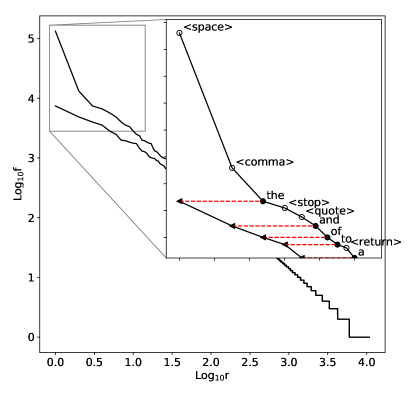
Figure 1: The translation of ranks for A Tale of Two Cities, by Charles Dickens. When both words and non-words are ranked by frequency (upper curve) the highest-frequency words emerge at rank 3—here, after space, and comma. When non-words are removed from the frequency ranking, all words are translated left (lower curve). This translation is highlighted in the inset zoom, where kept words move back along the red-dashed lines. Given the upper curve has a rank-frequency power law like Zipf’s (Eq. 1), the deletion of non-words (open circles) most significantly affects the lowest-ranked/highest-frequency words (solid circles), rolling back to the solid triangles, potentially related to Mandelbrot’s rank translation.

To understand any relationship between the shift by non-word deletion and Mandelbrot’s $k$, we need a method for $k$’s measurement. While the ZM law has a simple functional form, power-law regression is notably difficult. Accepted methodology for the determination of exponents centers around maximum likelihood estimation Clauset et al. (2009), although a number of other methodologies exist Gabaix and Ibragimov (2012); Virkar and Clauset (2014); Corral et al. (2015). However, we are not immediately interested in exponents or frequencies, but instead, ranks. Furthermore, optimization of $\gamma$ can obfuscate variation in $k$; $\gamma$ is well-known to be non-constant across ranks Ferrer-i-Cancho and Solé (2001); Montemurro (2001); Gerlach and Altmann (2013); Williams et al. (2015b), and is difficult to measure with precision Clauset et al. (2009). For these reasons, we fix $\gamma=1$ and switch to the rank domain for regression—the natural domain for $k$. While fixing $\gamma$ imposes bias in the measurement of $k$, it does so in a consistent way, allowing us to precisely understand $k$’s variation, which is all that is necessary for our study.

With $\gamma=1$, a quotient of Zipf’s law takes a convenient form: $\hat{y}_{\text{Z}}=\hat{f}_{\text{Z}}(w_{1})/\hat{f}_{\text{Z}}(w_{r})=r$. For the ZM law, the quotient becomes: $\hat{y}_{\text{ZM}}(w_{r})=(r+k)/(1+k)$. Defining $y(w_{r})=f(w_{1})/f(w_{r})$ for all $r$, the sum of squared errors: $\sum_{r=1}^{R}(y(w_{r})-\hat{y}_{\text{ZM}}(w_{r}))^{2}$ has analytic minimizer:

$$\hat{k}=\frac{\sum_{r=1}^{R}(r-1)^{2}}{\sum_{r=1}^{R}(r-1)(y(w_{r})-1)}.$$ (3)

This regression is convenient to our study for its analytic optimization. Not only does this avoid the possibility of multiple optimization minima, but efficiencies in its computation allow observation of $\hat{k}$ as a function of $R$.

To distinguish traditional word-frequency distributions from our space-integrated distributions we express the latter with $n$-ranks: $n=1,\cdots,N\geq R$; subscript models and parameters, e.g., $\hat{f}_{\text{S}}\propto(n+k_{\text{S}})^{-\gamma_{\text{S}}}$ for space’s integration; and write $n_{r}$ to indicate the space-integrated rank of the $r\textsuperscript{th}$ conventionally-ranked word. For a text that perfectly conforms to Zipf’s law and our dark-matter hypothesis, its space shift should be $\hat{k}_{\textsubscript{S}}=0$, making its ZM shift related to $n_{1}$, potentially as $\hat{k}_{\textsubscript{ZM}}\approx n_{1}-1$.

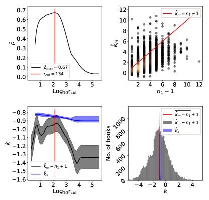
Figure 2: Top left: linear correlations between $\hat{k}_{\text{ZM}}$ and $n_{1}-1$ as a function of increasing cutoffs, $r_{\text{cut}}$. The maximum value, $\hat{\rho}_{\text{max}}\approx 0.67$, is observed over the ranks: $r=1,\cdots,r_{\text{cut}}=134$, indicated by vertical red line. Top right: scatter plot of $\hat{k}_{\text{ZM}}$ against $n_{1}-1$ for the maximizing cutoff with density indicated by shade: low to high/black to copper. A perfect relationship is indicated by the diagonal red line, which appears offset from the most dense region by a value near $1$. Bottom left: median offset (black line), $\hat{k}_{\text{ZM}}-n_{1}+1$, as a function of increasing cutoffs, $r_{\text{cut}}$, centered in the offset distribution’s middle decile (gray envelope). Offsets are compared to the median value for space-inclusive shifts (blue line), centered in the same distribution’s interquartile range. The same correlation-optimal cutoff is indicated by a vertical red line. Bottom right: histograms of $\hat{k}_{\text{ZM}}-n_{1}+1$ (gray) and $\hat{k}_{\text{S}}$ (blue) for the correlation-optimal cutoff, in addition to the average value of $\hat{k}_{\text{ZM}}-n_{1}+1$ (red line).

To investigate if $\hat{k}_{\textsubscript{ZM}}$ and $n_{1}-1$ covary we apply our rank regression to nearly $20,000$ English texts from the Project Gutenberg eBooks collection. We have used this data set in the past to explain tail behaviors of rank-frequency distributions. In this past study on text mixing Williams et al. (2015b) we showed how the compilation of documents into large, combined corpora leads to modulation of Zipf’s exponent, with more severe values of $\gamma>1$ at high ranks. The course of that study also led to our observation that many of the eBooks are themselves mixed. A notable example of our past study was the Complete Historical Romances of Georg Ebers, which is a compilation of over 100 short stories. The existence of these texts has a capacity to throw off regression of $\hat{k}_{\textsubscript{ZM}}$ in accommodation of the severe, mixing-derived exponents, $\gamma>1$. However, any true values of $k$ should be most apparent at smaller ranks Mandelbrot (1953), i.e., $r\rightarrow 1$. To separate the effects of secondary scalings at high ranks, $r\gg 1$, we explore an upper limit, $r\textsubscript{cut}\leq R$, on the number of terms in Eq. 3.

The results of our experiment are non-trivial. We $\rm{Log}$-space values of $r\textsubscript{cut}$ and measure the linear, Pearson correlations between $\hat{k}_{\textsubscript{ZM}}$ and $n_{1}-1$. While large cutoffs ($r\textsubscript{cut}\rightarrow R$) exhibit little-to-no association, we find a signal that is maximized near $r\textsubscript{cut}=100$, for which $\hat{\rho}\approx 0.67$. This is a strong correlation over nearly $20,000$ points, and even though we have performed multiple comparisons (676, for the $\rm{Log}$-spaced values of $r\textsubscript{cut}$), the low p-values observed (all p-values fell below $2\times 10^{-5}$) still test significant by the most stringent, Bonferroni correction Dunn (1961). This scan can be observed in Fig. 2 (top left), showing how strong correlations coincide with small cutoffs ($r\textsubscript{cut}<1,000$). For the optimal cutoff ($r\textsubscript{cut}=134$), we exhibit a scatter plot (Fig. 2, top right), highlighting how $\hat{k}_{\textsubscript{ZM}}$ increases with $n_{1}-1$, despite coarse, integer values of $n_{1}-1$. While these two quantities increase together, values of $n_{1}-1$ appear offset from $\hat{k}_{\textsubscript{ZM}}$ by a regular quantity near $1$. This deviation does not appear to be random, but is in fact in alignment with another quantity. In the lower-left panel of Fig. 2, variation (middle $10^{\text{th}}$ percentile, gray envelope) in the deviations, $\hat{k}_{\textsubscript{ZM}}-n_{1}+1$, is presented alongside variation (middle $50^{\text{th}}$ percentile, blue envelope) in the shift regressed from the space-inclusive frequency distribution, $\hat{k}_{\textsubscript{S}}$. Appearing much more stable than $\hat{k}_{\textsubscript{ZM}}$, values of $\hat{k}_{\textsubscript{S}}$ nearly align with the deviations at roughly the optimal cutoff. Thus, $\hat{k}_{\textsubscript{ZM}}$ is embedded with information that resolves the parameterization of the space-inclusive distribution, despite having no direct information on the presence of the excluded non-word objects! This result can be seen in the lower-right panel of Fig. 2, showing histograms of $\hat{k}_{\textsubscript{S}}$ and $\hat{k}_{\textsubscript{ZM}}-n_{1}+1$, where the variation in $\hat{k}_{\textsubscript{S}}$ is quite constrained, appearing like a vertical line.

While we have uncovered a strong signal relating the inclusion of non-words to Mandelbrot’s shift, this signal has appeared in a surprising manner. The space-inclusive distributions did not exhibit shift values close to zero, but instead extraordinarily regularly near a different value, $\hat{k}_{\textsubscript{S}}\approx-0.85$. The variation in this parameter is in fact far more narrow than that found for Zipf’s exponent Ferrer-i Cancho (2005); Williams et al. (2015a); Mehri and Jamaati (2017). Zipf’s scaling exponent, $\gamma$, is prone to mixing effects, which we have seen here to impact the space-exclusive shift ($\hat{k}_{\textsubscript{ZM}}$) when $r\textsubscript{cut}$ is roughly larger than $1000$. What makes $\hat{k}_{\textsubscript{S}}$ so much more robust than $\hat{k}_{\textsubscript{ZM}}$? At rank $n=1$, space is extraordinarily dominant in the frequency distributions, which is no surprise, since it acts as the primary word delimiter for English. More interestingly, though, is the range in which the very-regular, negative value that $\hat{k}_{\textsubscript{S}}$ assumes. Instead of describing a roll-back, $\hat{k}_{\textsubscript{S}}$ describes the opposite behavior—a disproportionately large quantity of high-frequency non-words. Unlike Mandelbrot’s roll-back, disproportionately high frequencies are actually predicted at these ranks by a generative mechanism.

The rank-frequency empiricism of the $20\textsuperscript{th}$ century was complimented by a stochastic model of language generation, defined by Herbert Simon Simon (1955). The goal of this endeavor was to go beyond observation of linguistic regularity to a mechanistic understanding of its production. Simon’s model relied on a fixed word-innovation rate: $\alpha$. With each time step, either a new word is drawn with probability $\alpha$, or an old word is drawn with probability $\theta=1-\alpha$. The choice of old words is based on an independence assumption: old words are drawn in proportion to their current frequencies. While Simon’s original analysis of this model identified a power-law frequency distribution of scaling exponent $\theta$, our recent work with this model Dodds et al. (2017) identified how as $\theta\rightarrow 1$, the frequency of the rank-$1$ word becomes disproportionately large. However, the disproportionate growth of this rank-$1$ outlier is not encoded by a piecewise functional form for frequency, but as we will show, a negative translation that is most impactive at small ranks. Thus, we now show how $\hat{k}_{\textsubscript{S}}$ is analytically predicted by Simon’s model, making space the run away, first mover of English language.

To exhibit Simon’s negative translation, we must define $M_{j}:j=1,\cdots,N$, as the step at which the $j\textsuperscript{th}$ word is innovated. Intuitively, $M_{j}$ is the number of words produced by the time the $j\textsuperscript{th}$ unique word appears. Previously Dodds et al. (2017), we determined the analytic form for the resulting frequency distribution:

$$\hat{f}(w_{j})=\frac{B(M_{j},\theta)}{B(M_{N},\theta)}\approx\left(\frac{M_{j}}{M_{N}}\right)^{-\theta}.$$ (4)

Using this, our piecewise ansatz for $M_{j}$: $M_{1}=1$; with $\langle M_{j}\rangle=(j-1)/\alpha$, for all $j>1$ exhibited a first mover’s disproportion, since the rank-1 word’s frequency was not damped by $\alpha$. In truth, this is not the real reason for the first mover’s dominance in Simon’s model. While near truth, our ansatz misses a key analytic feature that explains the first mover via a negative translation.

For any $j\geq 1$, $\langle M_{j+1}-M_{j}\rangle$ is the expectation of a geometric distribution with success probability $\alpha$, i.e., $\langle M_{j+1}-M_{j}\rangle=\alpha^{-1}$. Since one can show separation: $\langle M_{j+1}-M_{j}\rangle=\langle M_{j+1}\rangle-\langle M_{j}\rangle$, the resulting recursion equation: $\langle M_{j+1}\rangle=\langle M_{j}\rangle+\alpha^{-1}$ provides:

$$\langle M_{j}\rangle=\frac{\alpha+j-1}{\alpha}=\frac{j-\theta}{\alpha}.$$ (5)

While the first form in Eq. 5 exhibits the accuracy of our old ansatz, the latter will provide the most succinct and illustrative expression of frequency.

Approximation of $M_{j}$ by $\langle M_{j}\rangle=(j-\theta)/\alpha$ into both the numerator and denominator of Eq. 4 renders our refinement of the Simon model’s analytic frequencies:

$$\hat{f}(w_{j})\approx\left(\frac{j-\theta}{N-\theta}\right)^{-\theta}.$$ (6)

This unifies the Simon model’s frequencies into a common expression. For $j=1$, the negative shift by $\theta$ leaves $j-\theta=\alpha<1$ in the numerator, whose reciprocal ($\hat{f}$ is hyperbolic) can be large. This only occurs for the $j=1$, first mover, and since estimates Dodds et al. (2017) place $\theta$ near $1$, the entailed scaling outlier aligns with our empirical observations presented in Fig. 2. Thus, our empirical connection between Mandelbrot’s $k$ and the exclusion of non-words is simultaneously a smoking gun for Simon’s model as a primary mechanism for the generation of language (English, at least), i.e., our measurement of $\hat{k}_{\text{S}}$ tracks $\theta$, though not exactly, since we have forced $\gamma=1$.

So, what of languages other than English? Many utilize non-word delimiters similarly, and perhaps exhibit the space/first mover phenomenon. However, word segmentation is less trivial for a number of east-Asian languages, with space infrequent, in a diminished role. If Simon’s model applies to these, space’s sparsity as a delimiter and the absence of a dominant first mover should be apparent in values of $\hat{k}_{\text{S}}$ closer to zero (though still negative). This is an important avenue for study, and requires adequate word-segmentation tools, but is not the only question left open. Zipf studied other domains; e.g., do analogs for segmentation and dark matter exist and what would they mean for Zipfian city sizes Zipf (1949)?

Perhaps more immediately important is how our results may impact the language processing community. Excluding space from frequency analysis may be equivalent to ignoring the single most massive celestial object from a model of planetary motion. Could space’s inclusion have positive effects on the engineering side? Recently, we explored this possibility Williams (2017). Going beyond the incorporation of space, etc., we centered non-words as features in an algorithm. This algorithm is now state of the art for multiword expressions segmentation, thus an example for the practical integration of non-words. Furthermore, while many machine learning algorithms exclude stop words in preprocessing, Pennebaker Pennebaker (2011) exhibited how variation of pronouns and other high-frequency words is predictive of a variety of social and psychological characteristics. Regardless, this study provides a novel understanding of language, both in terms of empirical laws, and the nature of its formation.

The authors thank Sharon Williams for her thoughtful discussions, and gratefully acknowledge research support from Drexel University’s Department of Information Science and College of Computing and Informatics.

References

- Zipf (1949) G. K. Zipf, Human Behaviour and the Principle of Least-Effort (Addison-Wesley, 1949).
- Mandelbrot (1953) B. B. Mandelbrot, in Communication Theory, edited by B. W. Jackson (Butterworth, Woburn, MA, 1953), pp. 486–502.
- Simon (1955) H. A. Simon, Biometrika 42, 425 (1955).
- Miller (1957) G. A. Miller, American Journal of Psychology 70, 311 (1957).
- Li (1992) W. Li, IEEE Trans. Inf. Theor. 38, 1842 (1992).
- Corominas-Murtra et al. (2015) B. Corominas-Murtra, R. Handel, and S. Thurner, Proceedings of the National Academy of Sciences 112, 5348 (2015).
- Urzua (2000) C. M. Urzua, Economics Letters 66, 257 (2000).
- Clauset et al. (2009) A. Clauset, C. R. Shalizi, and M. E. J. Newman, SIAM Review 51, 661 (2009).
- Piantadosi (2014) S. T. Piantadosi, Psychonomic Bulletin & Review 21, 1112 (2014), ISSN 1069-9384, URL http://dx.doi.org/10.3758/s13423-014-0585-6.
- Gerlach and Altmann (2013) M. Gerlach and E. G. Altmann, Phys. Rev. X 3, 021006 (2013).
- Ferrer-i Cancho (2005) R. Ferrer-i Cancho, The European Physical Journal B - Condensed Matter and Complex Systems 44, 249 (2005).
- Ferrer-i-Cancho and Solé (2001) R. Ferrer-i-Cancho and R. V. Solé, Journal of Quantitative Linguistics 8, 165 (2001).
- Williams et al. (2015a) J. R. Williams, P. R. Lessard, S. Desu, E. M. Clark, J. P. Bagrow, C. M. Danforth, and P. S. Dodds, Nature Scientific Reports 5, 12209 (2015a).
- Williams et al. (2015b) J. R. Williams, J. P. Bagrow, C. M. Danforth, and P. S. Dodds, Physical Review E 91, 052811 (2015b).
- Kulig et al. (2017) A. Kulig, J. Kwapień, T. Stanisz, and S. Drożdż, Information Sciences 375, 98 (2017).
- Barabási and Albert (1999) A. L. Barabási and R. Albert, Science 286, 509 (1999).
- Krapivsky and Redner (2001) P. L. Krapivsky and S. Redner, Phys. Rev. E 63, 066123 (2001).
- Yule (1924) G. U. Yule, Phil. Trans. B 213, 21 (1924).
- Dodds et al. (2017) P. S. Dodds, D. R. Dewhurst, F. F. Hazlehurst, C. M. Van Oort, L. Mitchell, A. J. Reagan, J. R. Williams, and C. M. Danforth, Phys. Rev. E 95, 052301 (2017), URL https://link.aps.org/doi/10.1103/PhysRevE.95.052301.
- Mehri and Jamaati (2017) A. Mehri and M. Jamaati, Physical Letters A 381:31, 2470 (2017).
- Corral et al. (2015) A. Corral, G. Boleda, and R. Ferrer-i Cancho, PLOS ONE 10, 1 (2015).
- Gabaix and Ibragimov (2012) X. Gabaix and R. Ibragimov, Journal of Business & Economic Statistics 29, 24 (2012).
- Virkar and Clauset (2014) Y. Virkar and A. Clauset, The Annals of Applied Statistics 8, 89 (2014).
- Montemurro (2001) M. A. Montemurro, Physica A: Statistical Mechanics and Its Applications 300, 567 (2001).
- Dunn (1961) O. G. Dunn, Journal of the American Statistical Association 56, 52 (1961).
- Williams (2017) J. R. Williams, in In Proceedings of the 3rd Workshop on Noisy User Generated Text at the Conference on Empirical Methods in Natural Language Processing (2017).
- Pennebaker (2011) J. W. Pennebaker, The secret life of pronouns: what our words say about us (Bloomsbury Press, 2011).