The Effect of Crystal Symmetries on the Locality of Screw Dislocation Cores

Abstract

In linearised continuum elasticity, the elastic strain due to a straight dislocation line decays as $O(r^{-1})$, where $r$ denotes the distance to the defect core. It is shown in [7] that the core correction due to nonlinear and discrete (atomistic) effects decays like $O(r^{-2})$.

In the present work, we focus on screw dislocations under pure anti-plane shear kinematics. In this setting we demonstrate that an improved decay $O(r^{-p})$, $p>2$, of the core correction is obtained when crystalline symmetries are fully exploited and possibly a simple and explicit correction of the continuum far-field prediction is made.

This result is interesting in its own right as it demonstrates that, in some cases, continuum elasticity gives a much better prediction of the elastic field surrounding a dislocation than expected, and moreover has practical implications for atomistic simulation of dislocations cores, which we discuss as well.

35Q74, 49N60, 70C20, 74B20, 74G10, 74G65

1 Introduction

Crystalline solids consist of regions of periodic atom arrangements, which are broken by various types of defects. Crystalline defects can be separated into an elastic far-field which can normally be described by continuum linearised elasticity (CLE) and a defect core which is inherently atomistic and determines, for example, mobility, formation energy (and hence concentration), and so forth.

To make this idea concrete, let $\Lambda\subset\mathbb{R}^{d}$ be a crystalline lattice reference configuration and let $u:\Lambda\to\mathbb{R}^{d}$ be an equilibrium displacement field under some interaction law (see § 2.1). The point of view advanced in [7] is to decompose $u=u_{\rm ff}+u_{\rm core}$ where $u_{\rm ff}$ is a far-field predictor solving a CLE equation enforcing the presence of the defect of interest and $u_{\rm core}$ is a core corrector. For example, it is shown in [7] that for dislocations $|Du_{\rm ff}(x)|\sim|x|^{-1}$ while $|Du_{\rm core}(x)|\lesssim|x|^{-2}\log|x|$ where $D$ denotes a discrete gradient operator. The fast decay of the corrector $u_{\rm core}$ encodes the “locality” of the defect core (relative to the far-field).

The present work is the first in a series that introduces and developes techniques to substantially improve on the CLE far-field description. The overarching goal is to derive “higher-order” models for the far-field predictor $u_{\rm ff}$, which yield the same asymptotic behaviour as the CLE predictor (i.e., the same far-field boundary condition) but a more localised corrector. For example, in the case of a dislocation we seek $u_{\rm ff}$ such that $u=u_{\rm ff}+u_{\rm core}$ with $|Du_{\rm core}(x)|\lesssim|x|^{-p}$ and $p>2$. Constructions of this kind have a multitude of applications. They are interesting in their own right in that they give improved estimates on the region of validity of continuum mechanics. They may also be employed to more effectively construct models for multiple defects along the lines of [11]. A key motivation for us is that they yield a new class of boundary conditions for atomistic simulations that capture the far-field behaviour more accurately; this gives rise to improved algorithms for atomistic simulation defects; see § 3 for more detail.

In the present work, to demonstrate the potential of our approach and outline some of the key ideas required to carry out this programme, we focus on screw dislocations under anti-plane shear kinematics, in the cubic, hexagonal, and body-centred-cubic (BCC) lattices. The scalar setting, and the ability to exploit specific lattice symmetries, simplifies several constructions and proofs.

In forthcoming papers, in particular [2], we will discuss generalisations to vectorial deformations of general straight dislocations without any symmetry assumptions on the host crystal. In particular the absence of the symmetries we employ in the present work introduces a non-trival coupling between the core and the far-field predictor. The general idea that persists is that there is a development $u=u_{0}+u_{1}+\cdots+u_{n}+u_{\rm rem}$ of the solution, where the terms $u_{0},u_{1},\dots,u_{n}$ are given by simpler theories (e.g., linear PDEs) and the remainder $u_{\rm rem}$ has a higher decay rate.

Aside from providing a simplified introduction to [2], the present work contains results that are interesting in their own right due to the fact that anti-plane models of screw dislocations are particular popular in the mathematical analysis literature [1, 9, 11, 17] as a model problem for the more complex edge, mixed, and curved dislocations. Of particular note about our results here are:

(1) A combination of rotational and anti-plane reflection symmetries yield surprisingly high decay of the core corrector to the CLE predictor; see Theorem 2.7. This was numerically observed but unexplained in [11]. The key observation to obtain this result is that the CLE predictor satisfies additional PDEs, in particular the minimal surface equation, which naturally occurs in higher-order expansions of the atomistic forces.

(2) In a BCC crystal, due to the lack of anti-plane reflection symmetry, a nonlinear correction to the far-field predictor is required to improve the decay of the core corrector. One then expects that the dominant error contribution is the Cauchy–Born anti-discretisation error. The results of [3, 6, 15] suggest that the resultant corrector should decay as $O(\lvert x\rvert^{-3})$, however exploiting crystal symmetries reveals that the Cauchy–Born error is of higher order than expected and one even obtains a corrector decay of $O(\lvert x\rvert^{-4})$.

Finally, we remark that our analysis is carried out for short-ranged interatomic many-body potentials, however the resulting algorithms are applicable to electronic structure models rendering them an efficient and attractive alternative to complex and computationally expensive multi-scale schemes e.g, of atomistic/continuum or QM/MM type; see [5, 14] and references therein.

Outline: In Section 2 we describe in details our models and assumptions, and state our main results. Here, Section 2.2 is dedicated to the cubic and hexagonal lattice, while Section 2.3 discusses the BCC lattice. In Section 3 we present the resulting new numerical scheme including a convergence analysis. Our conclusions can be found in Section 4. Finally Section 5 contains the proofs of the main results.

2 Main results

2.1 Atomistic model for a screw dislocation

The atomistic reference configuration for a straight screw dislocation is given by a two-dimensional Bravais lattice $\Lambda=A_{\Lambda}\mathbb{Z}^{2}$, $A_{\Lambda}\in\mathbb{R}^{2\times 2}$ with $\det(A_{\Lambda})\neq 0$. In the present work we will only consider the triangular lattice and the square lattice, respectively given by

$$A_{\Lambda}=A_{\rm tri}:=\begin{pmatrix}1&\frac{1}{2}\\ 0&\frac{\sqrt{3}}{2}\end{pmatrix},\qquad A_{\Lambda}=A_{\rm quad}:=\begin{pmatrix}1&0\\ 0&1\end{pmatrix}.$$

The two-dimensional lattice $\Lambda$ should be thought of as the projection of a three-dimensional lattice: In case of an infinite straight dislocation in a three-dimensional lattice, the displacements do not depend on the dislocation line direction. Therefore, it suffices to consider the projected two-dimensional lattice.

Our atomistic model, which we specify momentarily, allows for general finite range interactions. All lattice directions included in the interaction range are encoded in a finite neighbourhood set $\mathcal{R}\subset\Lambda\backslash\{0\}$, which is fixed throughout. We always assume $\operatorname{span}_{\mathbb{Z}}\mathcal{R}=\Lambda$ and will specify further symmetry assumptions later on.

We consider an anti-plane displacement field $u\,:\,\Lambda\to\mathbb{R}$ and define $D_{\rho}u(x):=u(x+\rho)-u(x)$, $Du(x):=(D_{\rho}u(x))_{\rho\in\mathcal{R}}$, as well as the discrete divergence operator,

$$\operatorname{Div}g(x):=-\sum_{\rho\in\mathcal{R}}g_{\rho}(x-\rho)-g_{\rho}(x)\qquad\text{for any }g\colon\Lambda\to\mathbb{R}^{\mathcal{R}}.$$

In contrast to that we will always write $\nabla$ and $\operatorname{div}$ if we talk about the standard (continuum) gradient and divergence of differentiable maps.

A suitable function space for (relative) displacements is

$$\dot{\mathcal{H}}^{1}:=\{u\,:\,\Lambda\to\mathbb{R}\,|\,Du\in\ell^{2}(\Lambda)\}/\mathbb{R},$$

with norm

$$\|u\|_{\dot{\mathcal{H}}^{1}}:=\Big{(}\sum_{x\in\Lambda}\big{\lvert}Du(x)\big{\rvert}^{2}\Big{)}^{1/2}.$$

While we have factored out constants to make this a Banach space, we will often use the displacement $u$ and its equivalence class $[u]$ interchangeably when there is no risk of confusion.

For analytical purposes, we will also consider the space of compactly supported displacements

$$\mathcal{H}^{c}:=\{u\,:\,\Lambda\to\mathbb{R}\,|\,\operatorname{spt}(u)\text{ is bounded}\}.$$

Displacement fields containing dislocations do not belong to $\dot{\mathcal{H}}^{1}$ and the energy, naively written as a sum of local contributions, will be infinite. Following [7, 11] we therefore consider energy differences

(1) $$\mathcal{E}(u)=\sum_{x\in\Lambda}\Big{(}V(D\hat{u}(x)+Du(x))-V(D\hat{u}(x))\Big{)},$$

where $\hat{u}$ is a chosen far-field predictor that encodes the far-field boundary condition, while $u\in\dot{\mathcal{H}}^{1}$ is a core corrector to the given predictor so that $\hat{u}+u$ gives the overall displacement. We will minimise $\mathcal{E}(u)$ to equilibrate the defective crystal, but this requires some preparation first.

We assume throughout that $V\in C^{6}(\mathbb{R}^{\mathcal{R}},\mathbb{R})$ is a many-body potential encoding the local interactions. Examples of typical site potentials $V$ include Lennard-Jones type pair potentials (with cut-off) and EAM potentials; see also Section 2.3 and Section 3. With additional effort it would be possible to include simple quantum chemistry models within the framework [4], but to keep the presentation as simple as possible we will not pursue this in the current work.

As $\Lambda$ is either the square or triangular lattice, which are both invariant under certain symmetries, one is tempted to directly translate these symmetries to $\mathcal{R}$ and $V$. However, as mentioned above, $\Lambda$ should be seen as a projection of a three-dimensional lattice. Such a projection can add symmetries for the lattice that are not reflected in the interaction, since they are not symmetries of the underlying three-dimensional model. We will discuss such a case in detail in Section 2.3.

Because of this, we will only make the following reduced symmetry assumptions on $\mathcal{R}$ and $V$ throughout. Let $Q_{\Lambda}$ be the rotation by $\pi/2$ if $\Lambda=\mathbb{Z}^{2}$ and the rotation by $2\pi/3$ if $\Lambda=A_{\rm tri}\mathbb{Z}^{2}$. Then we assume that

(2) $$Q_{\Lambda}\mathcal{R}=\mathcal{R}\qquad\text{and}\qquad V(A)=V\left((A_{Q_{\Lambda}\rho})_{\rho\in\mathcal{R}}\right)\qquad\forall A\in\mathbb{R}^{\mathcal{R}}.$$

Since we only consider a plane orthogonal to the direction of the dislocation line, it is natural that the energy does not change if the displacements shifts an atom to its equivalent position in the plane above or below. Indeed we assume that there is a minimal periodicity $p>0$ such that

$$V(A)=V(A+p(\delta_{\rho\sigma})_{\sigma\in\mathcal{R}})\qquad\text{for all }A\in\mathbb{R}^{\mathcal{R}},\quad\rho\in\mathcal{R}.$$

The Burgers vector of a screw dislocation is then either $b=p$ or $b=-p$.

A key conceptual assumption that we require throughout this work is lattice stability (or, phonon stability): there exists $c_{0}>0$ such that

(3) $$\langle Hu,u\rangle\geq c_{0}\|u\|_{\dot{\mathcal{H}}^{1}}^{2}\qquad\forall u\in\dot{\mathcal{H}}^{1},$$

where $H$ denote the Hessian of the potential energy evaluated at the homogeneous lattice (note that this is different from $\delta^{2}\mathcal{E}(0)$),

$$\langle Hu,v\rangle=\sum_{x\in\Lambda}\sum_{\rho,\sigma\in\mathcal{R}}\nabla^{2}V(0)_{\rho\sigma}D_{\rho}u(x)D_{\sigma}v(x),\qquad\text{for }u,v\in\dot{\mathcal{H}}^{1}.$$

The choice of the predictor $\hat{u}$ in Eq. 1 for a specific problem is part of the modelling since it determines the far-field behaviour, e.g., it could encode an applied strain. Intuitively one can obtain a suitable $\hat{u}$ by solving a “simpler” model such as continuum linearised elasticity (CLE), which one expects to be approximately valid in the far-field; see [7] for a formalisation of this procedure.

Assume, for the time being, that $\hat{u}:\mathbb{R}^{2}\to\mathbb{R}$ is smooth away from a defect core $\hat{x}\in\mathbb{R}^{2}\setminus\Lambda$. Then, by employing Taylor expansions of both $\hat{u}$ and of $V$, we can approximate the atomistic force,

$$\frac{\partial\mathcal{E}}{\partial u(x)}\Big{|}_{u=0} =\Big{(}-\operatorname{Div}\nabla V(D\hat{u})\Big{)}(x)$$

(4) $$=-c\operatorname{div}\nabla W(\nabla\hat{u})+O(\nabla^{4}\hat{u}(x))+\text{h.o.t.s}$$

$$=-c\operatorname{div}(\nabla^{2}W(0)[\nabla\hat{u}])+O(\nabla^{4}\hat{u})+O(\nabla^{2}\hat{u}\nabla\hat{u})+\text{h.o.t.s},$$

where $W\,:\mathbb{R}^{2}\to\mathbb{R}$ is the Cauchy-Born energy per unit undeformed volume, defined by

(5) $$W(F):=\frac{1}{\det A_{\Lambda}}V(F\cdot\mathcal{R}).$$

Moreover, $O(\nabla^{4}\hat{u})$ represents the anti-discretisation error (note that the continuum model is now the approximation), $O(\nabla^{2}\hat{u}\nabla\hat{u})$ the linearisation error and “h.o.t.s” denotes additional terms that will be negligible in comparison.

It is therefore natural to solve a CLE model to obtain a far-field predictor for the atomistic defect equilibration problem for an anti-plane screw dislocation. Let $\hat{x}\in\mathbb{R}^{2}$ denote the dislocation core, then we define the branch cut (slip plane)

$$\Gamma:=\big{\{}(x_{1},\hat{x}_{2})\in\mathbb{R}^{2}\;|\;x_{1}\geq\hat{x}_{1}\big{\}}$$

and solve (we will see in Corollary 5.7 that under our general assumptions on $\mathcal{R}$ and $V$ we have $\nabla^{2}W(0)\propto\operatorname{Id}$)

(6a) $$-\Delta\hat{u} =0\quad\text{ in }\,\mathbb{R}^{2}\setminus\Gamma,$$

(6b) $$\hat{u}(x^{+})-\hat{u}(x^{-}) =-b\,\quad\text{ on }\,\Gamma\setminus\hat{x},$$

(6c) $$\partial_{x_{2}}\hat{u}(x^{+})-\partial_{x_{2}}\hat{u}(x^{-}) =0\,\quad\text{ on }\,\Gamma\setminus\hat{x}.$$

The system Eq. 6a–Eq. 6c has the well-known solution (cf. [8])

(7) $$\hat{u}(x)=\frac{b}{2\pi}\arg(x-\hat{x}),$$

where we identify $\mathbb{R}^{2}\cong\mathbb{C}$ and use $\Gamma-\hat{x}$ as the branch cut for $\arg$. Note for later use, that $\nabla\hat{u}\in C^{\infty}(\mathbb{R}^{2}\backslash\{0\})$ and $\lvert\nabla^{j}\hat{u}\rvert\lesssim\lvert x\rvert^{-j}$ for all $j\geq 0$ and $x\neq 0$.

As we want to study the effects of symmetry, we will assume throughout that the dislocation core $\hat{x}$ is, respectively, at the center of a triangle or square.

Having specified the far-field predictor we can now recall properties of the resulting variational problem.

Proposition 2.1.

Let $\hat{u}$ be given by Eq. 7, then $\mathcal{E}$ defined by Eq. 1 on $\mathcal{H}^{c}$ has a unique continuous extension $\mathcal{E}\colon\dot{\mathcal{H}}^{1}\to\mathbb{R}$. Furthermore, $\mathcal{E}\in C^{6}(\dot{\mathcal{H}}^{1})$.

Proof 2.2.

This is proven in [7, Lemma 3 and Remark 6].

Having established that $\mathcal{E}$ is well-defined, it is now meaningful to discuss the equilibration problem, either energy minimisers

(8) $$\bar{u}\in\arg\min_{\dot{\mathcal{H}}^{1}}\mathcal{E}$$

or, more generally, critical points

$$\delta\mathcal{E}(\bar{u})=0.$$

Critical points of the energy satisfy the following regularity and decay estimate.

Theorem 2.3.

If $[\bar{u}]\in\dot{\mathcal{H}}^{1}$ is a critical point of $\mathcal{E}$, then there exists $\bar{u}_{\infty}\in\mathbb{R}$ such that

$$\lvert D^{j}(\bar{u}(x)-\bar{u}_{\infty})\rvert\lesssim\lvert x\rvert^{-j-1}\log\lvert x\rvert,$$

for all $\lvert x\rvert$ large enough and $0\leq j\leq 4$.

Proof 2.4.

This result is proven in [7, Theorem 5 and Remark 9].

2.2 Anti-plane screw dislocations with mirror symmetry

The corrector decay rates in [7] are in general sharp (up to constants and log-factors), however the case of anti-plane screw dislocations appears to be an exception: In [11] it is seen numerically for a triangular lattice that, if the core is placed at the centre of a triangle, one approximately has $\lvert Du(x)\rvert\sim\lvert x\rvert^{-4}$ instead of the expected rate $\lvert x\rvert^{-2}\log\lvert x\rvert$. In the present section we relate this observation to several symmetry properties of the triangular lattice. We also discuss the square lattice case which shows a different behaviour to emphasise the importance of the triangular lattice.

These two-dimensional models represent a screw-dislocation in a cubic or hexagonal three-dimensional lattice only allowing for anti-plane displacements. In Section 2.3, we will additionally consider a BCC lattice and show how to derive these two-dimensional systems from the underlying three-dimensional model.

We recall that $\Lambda$ is either the square or triangular lattice which are both invariant under certain rotational symmetries. Crucially, we consider rotations about the dislocation core (not about a lattice site), which are described by the operators

$$L_{\Lambda}x:=Q_{\Lambda}(x-\hat{x})+\hat{x},$$

where $Q_{\Lambda}$ denotes a rotation through $\pi/2$ if $\Lambda=\mathbb{Z}^{2}$ and a rotation through $2\pi/3$ if $\Lambda=A_{\rm tri}\mathbb{Z}^{2}$. Since we assumed that $\hat{x}$ lies, respectively, at a center of triangle or square this implies $L_{\Lambda}\Lambda=\Lambda$.

In the present section we additionally assume mirror symmetry with respect to the plane orthogonal to the dislocation line, which is encoded in the site energy through the assumption

(9) $$V(A)=V(-A)\quad\text{for all }A\in\mathbb{R}^{\mathcal{R}}.$$

The mirror symmetry Eq. 9 is already implicit in our general assumptions for the square lattice (as it can be decomposed into a point reflection and an in-plane rotation by $\pi$). But it is an additional assumption for the triangular lattice. Here, it is equivalent to strengthen the rotational symmetry to rotations by $\pi/3$ instead of just $2\pi/3$.

Since $A$ represents an anti-plane displacement gradient $Du$, the map $A\mapsto-A$ does not represent a change in frame as it would in a full three-dimensional setting. In particular the derivation of $V$ for the BCC case in Section 2.3 shows that Eq. 9 is a non-trivial restriction on $V$.

Indeed, if one derives $V$ from an underlying three-dimensional site potential (see Section 2.3 for such a derivation in the case of a BCC lattice), then Eq. 9 means precisely that the three-dimensional lattice is mirror symmetric with respect to the plane orthogonal to the dislocation line. This is quite restrictive and effectively only true if the underlying three-dimensional lattice is given as $\Lambda^{\prime}=\Lambda\times\mathbb{Z}\subset\mathbb{R}^{3}$ which is a hexagonal or a cubic lattice for $\Lambda=A_{\rm tri}\mathbb{Z}^{2}$ or $\Lambda=\mathbb{Z}^{2}$, respectively.

In the next section Section 2.3, we will then consider a situation where Eq. 9 fails, by discussing a 111 screw dislocation in a BCC lattice.

Recall from Eq. 7 that the far-field predictor is given by $\hat{u}(x)=\frac{b}{2\pi}\arg(x-\hat{x})$. Since we now assume that $\hat{x}$ is at the centre of a square or triangle, $\hat{u}$ satisfies

(10) $$\hat{u}(L_{\Lambda}x) =\begin{cases}\hat{u}(x)+\frac{b}{3}\quad(\operatorname{mod}b),&\text{triangular lattice},\\ \hat{u}(x)+\frac{b}{4}\quad(\operatorname{mod}b),&\text{square lattice}.\\ \end{cases}$$

Motivated by this observation, we specify an analogous symmetry assumption on a general displacement.

Definition 2.5 (Inheritance of symmetries).

We say that a displacement $u$ inherits the rotational symmetry of $\hat{u}$ if

(11) $$u(L_{Q}x)=u(x)\quad\text{for all }x\in\Lambda.$$

Remark 2.6.

Inheritance of rotational (or other) symmetries would typically follow from the corresponding symmetries of $\hat{u},\Lambda,V$ and uniqueness of an energy minimiser (up to a global translation and lattice slips). However, due to the severe non-convexity of the energy landscape it cannot be expected in general. As an example, note that the line reflection symmetry in the BCC case, discussed in Section 2.3, is not necessarily inherited as is shown in [18].

We can now state the main results of this section. It is particularly noteworthy that they depend on the lattice under consideration. On a square lattice the symmetry only gives one additional order of decay compared to the decay rates in [7], while on a triangular lattice we do indeed show that there are two additional orders of decay as observed numerically in [11, Remark 3.7]. We will confirm this discrepancy in numerical tests in Section 3.

Theorem 2.7 (Decay with Mirror Symmetry).

Let $\Lambda\in\{\mathbb{Z}^{2},A_{\rm tri}\mathbb{Z}^{2}\}$ and suppose $\Lambda,\hat{x},\mathcal{R},V$ satisfy all the assumptions from Section 2.1. Furthermore, assume $V$ satisfies the mirror symmetry Eq. 9. If $\bar{u}$ is a critical point of $\mathcal{E}$ which inherits the rotational symmetry of $\hat{u}$, then we have for $j=1,2$ and all $\lvert x\rvert$ large enough

(12) $$\lvert D^{j}\bar{u}(x)\rvert\lesssim\lvert x\rvert^{-2-j}\log\lvert x\rvert,$$

if $\Lambda=\mathbb{Z}^{2}$, and

(13) $$\lvert D^{j}\bar{u}(x)\rvert\lesssim\lvert x\rvert^{-3-j}$$

for the triangular lattice $\Lambda=A_{\rm tri}\mathbb{Z}^{2}$.

Remark 2.8.

The result is also expected to hold for $j\geq 3$ and $j=0$ (up to subtracting a constant) following ideas in [7]. As we want to focus on other aspects and do not want to overburden the proof, this is omitted here.

Remark 2.9.

In the case of a triangular lattice the existence of a critical $u$ has been proven in [11] under severe restrictions on $V$. Under further restrictions it is even known to be a stable global minimiser. However it is unclear whether it inherits symmetry.

We emphasize, however, that the distinction between the hexagonal and BCC lattices, that is the loss of mirror symmetry in the BCC lattice was missed in [11]. Therefore, the results of [11] do not apply to the BCC case without further work.

Proof 2.10 (Idea of the proof of Theorem 2.7).

The full proof can be found in Section 5; here we only give a brief idea of the strategy.

Far from the defect core the equilibrium configuration is close to a homogeneous lattice, hence, the linearised problem becomes a good approximation. Therefore, a natural quantity to consider is the linear residual

(14) $$f_{u}=-\operatorname{Div}(\nabla^{2}V(0)[Du]).$$

On the one hand, one can recover $\bar{u}$ as a lattice convolution $\bar{u}=G\ast_{\Lambda}f_{\bar{u}}$ where $G$ is the fundamental solution, or Green’s function, of the linear atomistic equations. On the other hand, the decay of $f_{\bar{u}}$ can be estimated by Taylor expansion with the help of the nonlinear atomistic equations for $\hat{u}+\bar{u}$ and the continuum linear system for $\hat{u}$. In this expansion, $\nabla^{3}V(0)=0$ vanishes due to anti-plane symmetry, while the rotational symmetry leads to simple generic forms of higher order terms.

But even if $f_{\bar{u}}$ decays rapidly, this does not automatically translate to decay for $\bar{u}=G\ast f_{\bar{u}}$. Even if $f_{\bar{u}}$ has compact support $\bar{u}$ typically only inherits the decay of $G$. However, we show that, due to rotational symmetry, the first moment of $f_{\bar{u}}$ vanishes, while the second has a very special form. Improved estimates for the decay of $f_{\bar{u}}$ together with vanishing moments then lead to an improved rate of decay of $\bar{u}$.

The difference between the triangular lattice and the quadratic lattice lies in the form of the higher order terms in the expansion of $f_{\bar{u}}$. The terms in question are given by the atomistic-continuum error of the linear equation and by the nonlinearity $\nabla^{4}V(0)$. For the triangular lattice one finds the leading order expression $c_{1}\Delta^{2}\hat{u}$ for the linear and $c_{2}(g(x)\Delta\hat{u}+H(\hat{u}))$ for the nonlinear part, where only the constants $c_{1},c_{2}$ depend on the potentials. Here $H$ is the mean curvature of the graph $(x_{1},x_{2},\hat{u}(x))^{T}$. And the mean curvature vanishes as the graph is a helicoid, a minimal surface. Since $\Delta^{2}\hat{u}=0$, $\Delta\hat{u}=0$, and $H(\hat{u})=0$ all the leading order terms vanish. On the other hand, for the quadratic lattice, these terms are nontrivial and do not cancel.

2.3 Anti-plane screw dislocation in BCC

We turn towards the physically more important setting of a straight screw dislocation along the 111 direction in a BCC crystal. The three-dimensional BCC lattice can be defined by $\Lambda^{\prime\prime}=\mathbb{Z}^{3}+\{0,p\}$, with shift $p=\begin{pmatrix}\frac{1}{2}&\frac{1}{2}&\frac{1}{2}\\ \end{pmatrix}^{T}$. A screw dislocation along the 111 direction is obtained by taking both dislocation line and Burgers vector parallel to the vector $(1,1,1)^{T}$. If we rotate $\Lambda^{\prime\prime}$ by

$$Q=\frac{1}{\sqrt{6}}\begin{pmatrix}-1&-1&2\\ \sqrt{3}&-\sqrt{3}&0\\ \sqrt{2}&\sqrt{2}&\sqrt{2}\end{pmatrix}$$

and then rescale the lattice by $\sqrt{3/2}$, we obtain the three-dimensional Bravais lattice

$$\Lambda^{\prime}=\sqrt{3/2}Q\Lambda^{\prime\prime}=\begin{pmatrix}1&\frac{1}{2}&0\\ 0&\frac{\sqrt{3}}{2}&0\\ \frac{1}{2\sqrt{2}}&-\frac{1}{2\sqrt{2}}&\frac{3}{2\sqrt{2}}\end{pmatrix}\mathbb{Z}^{3}.$$

The 111 direction becomes the $e_{3}$ direction under this transformation, which is convenient for the subsequent discussion.

Since $p=\frac{3}{2\sqrt{2}}$, the Burgers vector is now given by $b=\pm\frac{3}{2\sqrt{2}}$ (corresponding to the actual Burgers vector in three dimensions being $(0,0,b)^{T}$). We project the BCC lattice $\Lambda^{\prime}$ along the dislocation direction $e_{3}$ to obtain the triangular lattice

$$\Lambda=\big{\{}(x_{1},x_{2})\,\big{|}\,x\in\Lambda^{\prime}\big{\}}=A_{\rm tri}\mathbb{Z}^{2}.$$

Note though that these projections correspond to different “heights”, i.e., different $z$-coordinates in $\Lambda^{\prime}$. Indeed, it is helpful to split $\Lambda$ into the three lattices $\Lambda=\Lambda_{1}\cup\Lambda_{2}\cup\Lambda_{3}$, where

$$\Lambda_{i}=v_{i}+\begin{pmatrix}\frac{3}{2}&\frac{3}{2}\\ \frac{\sqrt{3}}{2}&-\frac{\sqrt{3}}{2}\end{pmatrix}\mathbb{Z}^{2},$$

with $v_{1}=0$, $v_{2}=e_{1}$, $v_{3}=\begin{pmatrix}\frac{1}{2}&\frac{\sqrt{3}}{2}\end{pmatrix}^{T}$. In this notation, one can recover the three-dimensional lattice as

$$\Lambda^{\prime}=\bigcup_{i}\Big{(}\Lambda_{i}\times\Big{\{}\Big{(}k+\frac{i}{3}\Big{)}\frac{3}{2\sqrt{2}}\colon k\in\mathbb{Z}\Big{\}}\Big{)}.$$

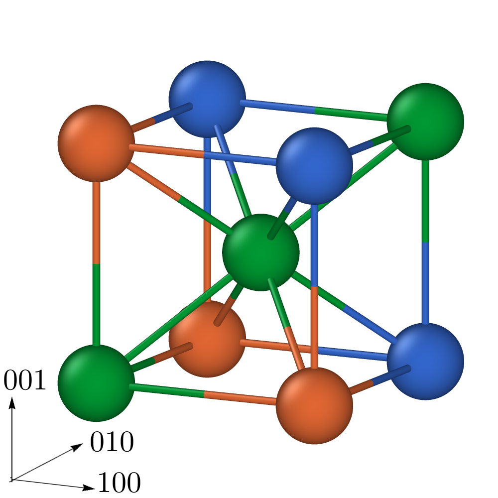
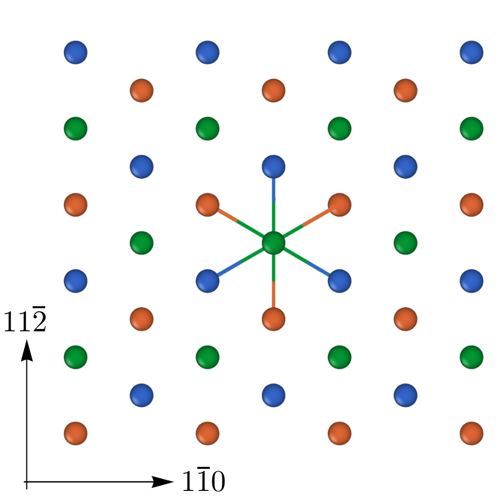
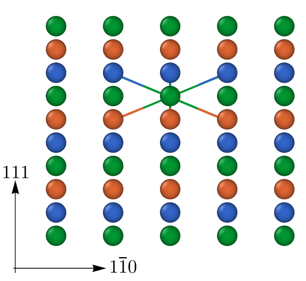
Figure 1: Consider the middle green atom in the BCC unit cube (left picture). After projecting along the 111-direction (the green diagonal), the three green atoms are represented as one, which has six other-coloured atoms in the unit cube as its nearest-neighbours (middle picture). The different heights of atomic planes associated with each colour are best seen by projecting the same lattice along the $11\overline{2}$-direction (right picture).

Next, we formally derive an anti-plane interatomic potential as a projection from a three-dimensional model. The derivation is only formal as many of the sums appearing are infinite if summed over the entire lattice. Indeed, for a deformation $y$ consider formally

$$\mathcal{E}^{\rm 3d}(y)=\sum_{x\in\Lambda^{\prime}}V^{\prime}(D^{\prime}y(x)),$$

where $D^{\prime}y(x)=(D_{\rho}y(x))_{\rho\in\Lambda^{\prime}}$ and $V^{\prime}\colon\mathbb{R}^{3\times\Lambda^{\prime}}\to\mathbb{R}$. Note that, to achieve the periodicity of $V$ (slip invariance) $V^{\prime}$ must depend on the entire crystal. However, it is convenient to assume that it has a finite cut-off $d>0$ such that $V^{\prime}(A)=V^{\prime}(B)$ whenever $A,B$ satisfy $A_{\rho}=B_{\rho}$ for all $\rho$ with $\lvert A_{\rho}\rvert<d$ or $\lvert B_{\rho}\rvert<d$.

In contrast to $\mathcal{E}$, $\mathcal{E}^{\rm 3d}$ acts on deformations instead of displacements. To derive an energy on anti-plane displacements, we consider deformations of the form

$$y^{u}:\Lambda^{\prime}\to\mathbb{R}^{3},\qquad y^{u}(x):=\big{(}x_{1},x_{2},x_{3}+u(x_{1},x_{2})\big{)}$$

for anti-plane displacements $u:\Lambda\to\mathbb{R}$. As differences of $y^{u}$ do not depend on $x_{3}$, the same is true for the local energy contributions. Therefore, we can formally renormalise the (possibly infinite) energy to

$$\mathcal{E}^{\rm 3d}_{\rm norm}(u)=\sum_{x\in\Lambda^{\prime}\cap(\mathbb{R}^{2}\times[0,p))}V^{\prime}(D^{\prime}y^{u}(x)),$$

the energy per periodic layer of thickness $p$. Since $\lvert D_{\rho}y^{u}(x)\rvert\geq\lvert(\rho_{1},\rho_{2})\rvert$, the local energy at any $x$ can only depend on the projected directions $\mathcal{R}:=\Lambda\cap B_{d}(0)\backslash\{0\}$. We can therefore define

$$V(Du(x_{1},x_{2})):=V^{\prime}(D^{\prime}y^{u}(x)),$$

for $x\in\Lambda^{\prime}$, to obtain $\mathcal{E}(u)=\mathcal{E}^{\rm 3d}_{\rm norm}(y^{u})$.

Of course we assume that $V^{\prime}$ is frame-indifferent, $V^{\prime}(QA)=V^{\prime}(A)$ for all $A$ and $Q\in\operatorname{O}(3)$. Furthermore, we assume that $V^{\prime}$ is invariant under relabelling of atoms (permutation invariance). In particular, this means that $V^{\prime}$ is compatible with the lattice symmetries of $\Lambda^{\prime}$: $V^{\prime}(A)=V^{\prime}((A_{-\rho})_{\rho\in\Lambda^{\prime}})$ and $V^{\prime}(A)=V^{\prime}((A_{Q^{\prime}\rho})_{\rho\in\Lambda^{\prime}})$, where $Q^{\prime}$ is the rotation through $2\pi/3$ with axis $e_{3}$. $\Lambda^{\prime}$ is also invariant under line reflection symmetry with respect to the line spanned by $a^{\prime}=(\frac{\sqrt{3}}{2},\frac{1}{2},0)^{T}$. Denoting the reflection map by $S^{\prime}$ we thus have $V^{\prime}(A)=V^{\prime}((A_{S^{\prime}\rho})_{\rho\in\Lambda^{\prime}})$.

We can now translate these properties to symmetries of $V$. Clearly, $\mathcal{R}=-\mathcal{R}$ and $Q_{\Lambda}\mathcal{R}=\mathcal{R}$. The symmetry properties of $V^{\prime}$ directly imply $V(A)=V\left((A_{Q_{\Lambda}\rho})_{\rho\in\mathcal{R}}\right)$ and $V(A)=V\left((-A_{-\rho})_{\rho\in\mathcal{R}}\right)$ for all $A\in\mathbb{R}^{\mathcal{R}}$. The slip invariance $V(A)=V(A+p(\delta_{\rho\sigma})_{\sigma\in\mathcal{R}})$ also follows from permutation invariance of $V^{\prime}$. We have thus obtained all the general assumptions that we imposed on $V$ in Section 2.1.

Additionally, we will exploit the line reflection symmetry. Let $a=(\frac{\sqrt{3}}{2},\frac{1}{2})^{T}$. A reflection at the line spanned by $a$ in $\mathbb{R}^{2}$ is given by

$$S=a\otimes a-a^{\bot}\otimes a^{\bot}=\begin{pmatrix}\frac{1}{2}&\frac{\sqrt{3}}{2}\\ \frac{\sqrt{3}}{2}&-\frac{1}{2}\end{pmatrix}.$$

Due to the line reflection symmetry described by $S^{\prime}$ as well as frame-indifference with $Q=S^{\prime}$, we deduce

(15) $$S\mathcal{R}=\mathcal{R},\quad\text{and}\quad V(A)=V\left((-A_{S\rho})_{\rho\in\mathcal{R}}\right).$$

We emphasize that $\Lambda^{\prime}$ is not invariant under a rotation by only $\pi/3$ around the axis $e_{3}$. This is easily seen, as this rotation maps $\Lambda_{2}$ to $\Lambda_{3}$ and vice versa. Equivalently, it is not invariant under the mirror symmetry $x\mapsto(x_{1},x_{2},-x_{3})^{T}$ expressed by Eq. 9. Therefore, the more specific results from the previous section, Section 2.2, do not apply.

While in the setting of Section 2.2 screw dislocations with Burgers vector $b=p$ and $b=-p$ are equivalent, the loss of mirror symmetry in the BCC crystal also creates two distinctively different screw dislocations, the so-called easy and hard core. In particular, they have a different core structure; see e.g. [12].

The improved decay rates we obtained in Section 2.2 no longer hold up either. Indeed, one can see in numerical calculations, see Section 3, that the $\lvert x\rvert^{-2}$ bound on the decay of the strains is sharp (up to logarithmic terms and constants).

Our aim now, as announced in the Introduction, is to develop a new far-field predictor so that the corresponding corrector recovers the higher $\lvert x\rvert^{-4}$ accuracy of the more symmetric case. A natural first idea is to replace CLE with the Cauchy–Born nonlinear elasticity equation, however, these are not easy to solve analytically. Instead, we expand the solution $u=\hat{u}+u_{1}+u_{2}+\dots$ hoping for $\nabla^{j}u_{2}\ll\nabla^{j}u_{1}\ll\nabla^{j}\hat{u}$, which yields

$$\operatorname{div}\nabla W(\nabla u)\sim\, \operatorname{div}\nabla^{2}W(0)\nabla\hat{u}$$

$$+\operatorname{div}\Big{(}\nabla^{2}W(0)\nabla u_{1}+\frac{1}{2}\ \nabla^{3}W(0)[\nabla\hat{u},\nabla\hat{u}]\Big{)}$$

$$+\operatorname{div}\Big{(}\nabla^{2}W(0)\nabla u_{2}+\nabla^{3}W(0)[\nabla\hat{u},\nabla u_{1}]+\nabla^{4}W(0)[\nabla\hat{u},\nabla\hat{u},\nabla\hat{u}]\Big{)}+\dots.$$

The atomistic-continuum error is typically expected to be of comparable size as the last terms. But, as the projected lattice is still a triangular lattice, many of the arguments discussed in Section 2.2 still apply and the highest order of this error as well as the term $\nabla^{4}W(0)[\nabla\hat{u},\nabla\hat{u},\nabla\hat{u}]$ vanish. However, we now have $\nabla^{3}W(0)\neq 0$ making the remaining terms non-trivial. We can thus obtain the first two corrections to $\hat{u}$ by solving the linear PDEs

(16a) $$-\operatorname{div}\nabla^{2}W(0)\nabla u_{1} =\frac{1}{2}\operatorname{div}\Big{(}\nabla^{3}W(0)[\nabla\hat{u},\nabla\hat{u}]\Big{)},$$

(16b) $$-\operatorname{div}\nabla^{2}W(0)\nabla u_{2} =\operatorname{div}\Big{(}\nabla^{3}W(0)[\nabla\hat{u},\nabla u_{1}]\Big{)}$$

on $\mathbb{R}^{2}\backslash\{0\}$.

Due to Corollaries 5.7 and 5.9, exploiting the rotational crystalline symmetry, we can simplify them as

(17a) $$-c_{\rm lin}\Delta u_{1} =c_{\rm quad}\begin{pmatrix}\partial_{11}\hat{u}-\partial_{22}\hat{u}\\ -2\partial_{12}\hat{u}\end{pmatrix}\cdot\nabla\hat{u},$$

(17b) $$-c_{\rm lin}\Delta u_{2} =c_{\rm quad}\bigg{(}\begin{pmatrix}\partial_{11}u_{1}-\partial_{22}u_{1}\\ -2\partial_{12}u_{1}\end{pmatrix}\cdot\nabla\hat{u}+\begin{pmatrix}\partial_{11}\hat{u}-\partial_{22}\hat{u}\\ -2\partial_{12}\hat{u}\end{pmatrix}\cdot\nabla u_{1}\bigg{)}.$$

where

$$c_{\rm lin} =\frac{1}{2}\operatorname{tr}\nabla^{2}W(0),\qquad\text{and}$$

$$c_{\rm quad} =\frac{1}{4}(\nabla^{3}W(0)_{111}-3\nabla^{3}W(0)_{122}).$$

In polar coordinates, $x=\hat{x}+r(\cos\varphi,\sin\varphi)$, using the fact that $\hat{u}=\frac{b}{2\pi}\arg(x-\hat{x})=\frac{b}{2\pi}\varphi$, Eq. 17a becomes

$$-\Delta u_{1}=\frac{c_{\rm quad}b^{2}}{c_{\rm lin}2\pi^{2}}\frac{\cos(3\varphi)}{r^{3}},$$

from which we readily infer that one possible solution is

(18) $$u_{1}(x+\hat{x})=\frac{c_{\rm quad}b^{2}}{c_{\rm lin}16\pi^{2}}\frac{\cos(3\varphi)}{r}=\frac{c_{\rm quad}b^{2}}{c_{\rm lin}16\pi^{2}}\frac{x_{1}^{3}-3x_{1}x_{2}^{2}}{\lvert x\rvert^{4}}.$$

Similarly, inserting $\hat{u}$ and $u_{1}$ into Eq. 17b yields

$$-\Delta u_{2}=\frac{c_{\rm quad}^{2}b^{3}}{c_{\rm lin}^{2}4\pi^{3}}\frac{\sin(6\varphi)}{r^{4}},$$

for which a solution is given by

(19) $$u_{2}(x+\hat{x})=\frac{c_{\rm quad}^{2}b^{3}}{c_{\rm lin}^{2}128\pi^{3}}\frac{\sin(6\varphi)}{r^{2}}=\frac{c_{\rm quad}^{2}b^{3}}{c_{\rm lin}^{2}128\pi^{3}}\frac{6x_{1}^{5}x_{2}-20x_{1}^{3}x_{2}^{3}+6x_{1}x_{2}^{5}}{\lvert x\rvert^{8}}.$$

While there are many more solutions for both problems, we will choose these specific ones as they satisfy the decay estimates

(20) $$\lvert\nabla^{j}u_{i}\rvert\lesssim\lvert x\rvert^{-i-j}$$

and the rotational symmetry $u_{i}(L_{Q}x)=u_{i}(x)$. With the solutions $u_{1}$ and $u_{2}$ obtained, respectively, in Eqs. 18 and 19 we obtain the following result.

Theorem 2.11 (BCC).

Let $\Lambda=A_{\rm tri}\mathbb{Z}^{2}$ and suppose $\Lambda,\hat{x},\mathcal{R},V$ satisfy all the assumptions from Section 2.1. Furthermore, assume $\mathcal{R}$ and $V$ satisfy the line reflection symmetry Eq. 15. Consider a critical point $\bar{u}$ of Eq. 1 that inherits the rotational symmetry of $\hat{u}$. Then we can write $\bar{u}=u_{1}+u_{2}+\bar{u}_{\rm rem}$ where $u_{1}$ and $u_{2}$ are given by Eq. 18 and Eq. 19 and the remainder $\bar{u}_{\rm rem}$ satisfies the decay estimates

(21) $$\lvert D^{j}\bar{u}_{\rm rem}(x)\rvert\lesssim\lvert x\rvert^{-j-3}\log\lvert x\rvert,$$

for $j=1,2$ and all $\lvert x\rvert$ large enough.

Remark 2.12.

As discussed in the introduction, our new predictor $\hat{u}+u_{1}+u_{2}$ does not just result in $O(\lvert x\rvert^{-3})$ accuracy for the strain which one might expect from the general expansion idea or from well-established results about the Cauchy-Born anti-discretisation error. The actual accuracy is one order higher, i.e., $O(\lvert x\rvert^{-4})$.

Remark 2.13.

Since $|D^{j}u_{1}(x)|\lesssim|x|^{-j-1}$, without log-factors, Theorem 2.11 improves the result of Theorem 2.3 to

$$\big{|}D^{j}\bar{u}(x)\big{|}\lesssim|x|^{-j-1},\qquad j=1,2.$$

3 Numerical approximation

3.1 Supercell approximation

A central motivation for the present work are the poor convergence rates of standard supercell approximations for the defect equilibration problem Eq. 8 established in [7]. We can now exploit the theoretical results from Section 2 to construct boundary conditions that give rise to new supercell approximations. These have improved rates of convergence without any corresponding increase in computational complexity.

We begin by defining a generalised energy-difference functional in a predictor-corrector form

$$\mathcal{E}(u_{\rm pred};u):=\sum_{x\in\Lambda}V\big{(}Du_{\rm pred}(x)+Du(x)\big{)}-V\big{(}Du_{\rm pred}(x)\big{)},$$

$$\text{for }u_{\rm pred}\in\hat{u}+\dot{\mathcal{H}}^{1},u\in\dot{\mathcal{H}}^{1}.$$

Then, the generalised variational problem

(22) $$\tilde{u}\in\arg\min\big{\{}\mathcal{E}(u_{\rm pred};u)\,|\,u\in\dot{\mathcal{H}}^{1}\big{\}}$$

is equivalent to Eq. 8, via the identity $u_{\rm pred}+\tilde{u}=\hat{u}+\bar{u}$.

We now note as in [7] that the supercell approximation on a domain $B_{R}\cap\Lambda\subset\Omega_{R}\subset\Lambda$ with boundary condition $u_{\rm pred}$ on $\Lambda\setminus\Omega_{R}$ can be written as a Galerkin approximation

(23) $$\tilde{u}_{R}\in\arg\min\big{\{}\mathcal{E}(u_{\rm pred};u)\,|\,u\in\mathcal{H}^{0}(\Omega_{R})\big{\}},$$

where $$\mathcal{H}^{0}(\Omega_{R}):=\{v\in\mathcal{H}^{c}\,|\,v=0\,\text{ in }\,\Lambda\setminus\Omega_{R}\}.$$

Using generic properties of Galerkin approximations we obtain the following approximation error estimate.

Theorem 3.1.

Let $\tilde{u}$ be a strongly stable solution (cf. [7]) to Eq. 22, i.e. satisfying

$$\delta_{u}^{2}\mathcal{E}(u_{\rm pred};\tilde{u})[v,v]\geq C\|v\|_{\dot{\mathcal{H}}^{1}}^{2},$$

for all $v\in\mathcal{H}^{c}$. If $\tilde{u}$ further satisfies

$$|D\tilde{u}(x)|\lesssim|x|^{-s}\log^{r}|x|,$$

for some $s>1,r\in\{0,1\}$, then there exist $C,R_{0}>0$ such that, for all $R>R_{0}$ there exists a stable solution $\tilde{u}_{R}$ to Eq. 23 satisfying

(24) $$\|\tilde{u}_{R}-\tilde{u}\|_{\dot{\mathcal{H}}^{1}}\leq CR^{-s+1}\log^{r}(R).$$

Proof 3.2.

The existence of a solution $\tilde{u}_{R}$, for $R$ sufficiently large, follows from [7, Theorem 6] (the case $u_{\rm pred}=\hat{u}$) and the equivalence of Eq. 22 with Eq. 8. Moreover, following the proof of [7, Theorem 6] verbatim we obtain

$$\|\tilde{u}_{R}-\tilde{u}\|_{\dot{\mathcal{H}}^{1}}\lesssim\|\tilde{u}\|_{\dot{\mathcal{H}}^{1}(\Lambda\setminus B_{R/2})}.$$

We then apply the assumption that $|D\tilde{u}(x)|\lesssim|x|^{-s}\log^{r}|x|$ to arrive at the desired error estimate,

$$\|\tilde{u}_{R}-\tilde{u}\|_{\dot{\mathcal{H}}^{1}}\lesssim\bigg{(}\sum_{x\in\Lambda\setminus B_{R/2}}|D\tilde{u}(x)|^{2}\bigg{)}^{1/2}\lesssim R^{1-s}\log^{r}(R).$$

3.2 Numerical examples with mirror symmetry

To test the results from Section 2.2 we consider a toy model involving nearest-neighbour pair interaction,

$$V(Du(x))=\sum_{\rho\in\mathcal{R}}\psi(D_{\rho}u(x)),\qquad\psi(r)=\sin^{2}(\pi r),$$

which is $1$-periodic, i.e., $p=1$. We investigate the three cases

1. symmetric square:
   $\Lambda=\mathbb{Z}^{2},\quad\mathcal{R}=\{\pm e_{1},\pm e_{2}\},\quad\hat{x}=\left(\frac{1}{2},\frac{1}{2}\right)$;

2. symmetric triangular:
   $\Lambda=A_{\rm tri}\mathbb{Z}^{2},\quad\mathcal{R}=\left\{\pm\begin{pmatrix}1\\ 0\end{pmatrix},\pm\begin{pmatrix}\frac{1}{2}\\ \frac{\sqrt{3}}{2}\end{pmatrix},\pm\begin{pmatrix}-\frac{1}{2}\\ \frac{\sqrt{3}}{2}\end{pmatrix}\right\},\quad\hat{x}=\left(\frac{1}{2},\frac{\sqrt{3}}{6}\right)$;

3. asymmetric triangular: as in (ii), but with $\hat{x}=\left(\frac{1}{4},\frac{1}{8}\right)$.

The cases (i) and (ii) satisfy all conditions of Theorem 2.7 while (iii) fails the crucial symmetry assumptions. In particular, at least up to logarithmic terms, our theory predicts $\lvert D\bar{u}(x)\rvert\lesssim\lvert x\rvert^{-3}$ for (i), $\lvert D\bar{u}(x)\rvert\lesssim\lvert x\rvert^{-4}$ for (ii), and $\lvert D\bar{u}(x)\rvert\lesssim\lvert x\rvert^{-2}$ for (iii). Due to Theorem 3.1 this corresponds to $\|\tilde{u}_{R}-\tilde{u}\|_{\dot{\mathcal{H}}^{1}}$ being $O(R^{-2})$, $O(R^{-3})$, and $O(R^{-1})$, respectively. To compute equilibria we employ a standard Newton scheme, terminated at an $\ell^{\infty}$-residual of $10^{-8}$. In Figure 2 we plot both the decay of the correctors, confirming the predictions of Theorem 2.7, and the approximation error in the supercell approximation against the domain size $R$, confirming the prediction of Theorem 3.1.

Remark 3.3.

An asymmetric square case (that is as in (i) but with $\hat{x}=\left(\frac{1}{3},\frac{1}{3}\right)$ has also been considered and the results are as expected by our theory and thus are qualitatively equivalent to (iii). Therefore we do not include them in the figures to retain clarity. It does however further emphasise the role of symmetry in the problem.

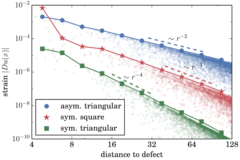
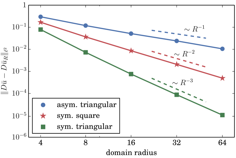
Figure 2: Left: Decay of $|D\bar{u}|$ for the triangular and square lattices, with and without rotational symmetry. Transparent dots denote data points $(|x|,|Du(x)|)$, solid curves their envelopes. We observe the improved decay rates $r^{-3}$ and $r^{-4}$, proven in Theorem 2.7, when the dislocation core is chosen as a high symmetry point.
                                                                                                                                   Right: Rates of convergence of the supercell approximation Eq. 23 in the three cases specified in Section 3.2. We observe the improved rates of decay of the corrector in the high symmetry cases as predicted by Theorem 3.1.

3.3 Numerical example in BCC Tungsten

To confirm the result of Section 2.3, we consider a Finnis–Sinclair type model (EAM model) for BCC Tungsten (W), where the 3D site energy for a deformation $y$ is of the form

$$V^{\prime}(D^{\prime}y)=-\Big{(}\sum_{\sigma\in\Lambda^{\prime}}\rho\big{(}|D_{\sigma}y|\big{)}\Big{)}^{1/2}+\sum_{\sigma\in\Lambda^{\prime}}\phi\big{(}|D_{\sigma}y|\big{)},$$

and the electron density $\rho$ and pair repulsion $\phi$ are obtained from [18]. The projected anti-plane model is then constructed as described in Section 2.3. The supercell model Eq. 23 is solved to within an $\ell^{\infty}$ residual of $10^{-6}$ using a preconditioned LBFGS algorithm [16].

We investigate two test cases, the easy dislocation core (negatively oriented) and the hard dislocation core (positively oriented), cf. [12]. For each case, following Section 2.3, we consider three different predictors:

1. standard linearised elasticity predictor (0th order), i.e., $u_{\rm pred}=\hat{u}$;

2. 1st order correction, i.e. $u_{\rm pred}=\hat{u}+u_{1}$;

3. 2nd order correction, i.e. $u_{\rm pred}=\hat{u}+u_{1}+u_{2}$,

with $\hat{u}$ given in Eq. 7 and $u_{1},u_{2}$, respectively, in Eq. 18 and Eq. 19.

In Figures 4 and 3 on the left-hand side we display the decay of the correctors for, respectively, the hard (positive) and easy (negative) dislocation cores, confirming the prediction of Theorem 2.11. On the right-hand side we plot the corresponding approximation errors in the supercell approximation against the domain size $R$, confirming the prediction of Theorem 3.1.

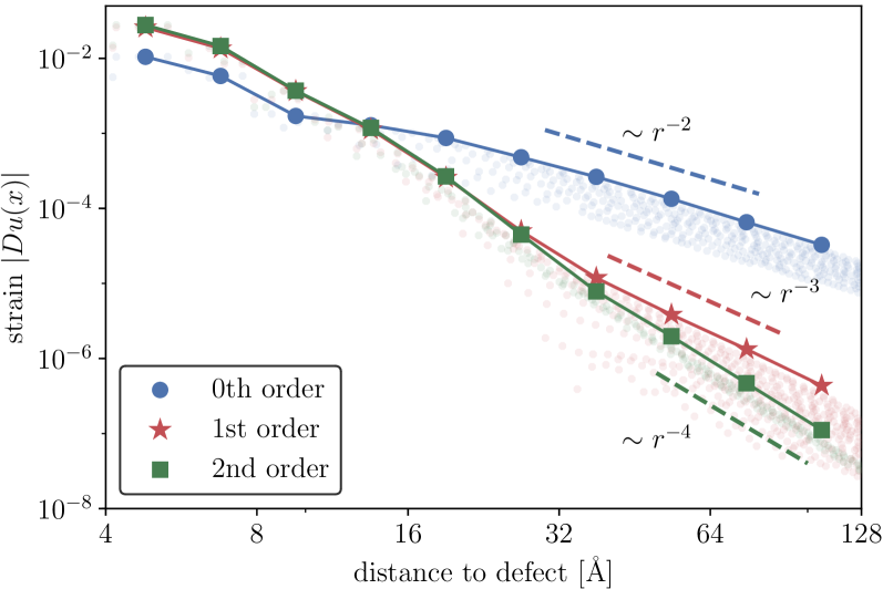
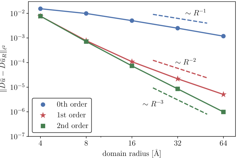
Figure 3: Left: Decay of $|D\bar{u}|$ for a BCC easy core screw dislocation with standard and improved far-field predictors; cf. Section 3.3. Transparent dots denote data points $(|x|,|Du(x)|)$, solid curves their envelopes. The numerically observed improved decay for higher-order predictors is consistent with Theorem 2.11.
                                                                                                                                   Right: Rates of convergence of the supercell approximation Eq. 23 to the BCC easy core screw dislocation, employing the standard as well as higher-order far-field predictors. The improved rates of convergence due to the faster decay of the corrector solutions are consistent with Theorem 3.1.

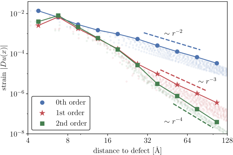
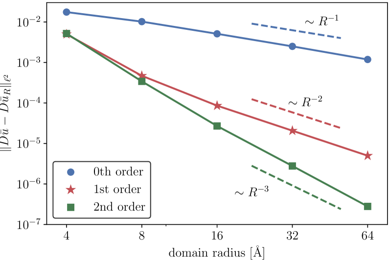
Figure 4: Left: Decay of $|D\bar{u}|$ for a BCC hard core screw dislocation with standard and improved far-field predictors; cf. Section 3.3. Transparent dots denote data points $(|x|,|Du(x)|)$, solid curves their envelopes. The numerically observed improved decay for higher-order predictors is consistent with Theorem 2.11.
                                                                                                                                   Right: Rates of convergence of the supercell approximation Eq. 23 to the BCC hard core screw dislocation, employing the standard as well as higher-order far-field predictors. The improved rates of convergence due to the faster decay of the corrector solutions are consistent with Theorem 3.1.

4 Conclusion

We have developed a range of results establishing finer properties of the elastic far-field generated by a screw dislocation in anti-plane shear kinematics. Of particular note is the role that crystalline symmetries play in obtaining either cancellation (screw and square lattice) or simple and explicit representations of the leading order terms of this elastic far-field. As a key application we showed how these results can be exploited to obtain boundary conditions with significantly improved convergence rates in terms of computational cell size.

Most importantly, though, the general ideas that we outlined in this paper set the scene for an in-depth study of the elastic far-field for a large variety of defect types, fully vectorial models, and more general crystalline solids. The resulting derivation of higher-order boundary conditions promises to yield simple, efficient as well as highly accurate new algorithms to simulate crystalline defects.

5 Proofs

5.1 Auxiliary results about symmetry

We prove the main results through a number of lemmas, starting with the following observations about how symmetry simplifies the tensors appearing in the development of the forces. This includes, but is not limited to the tensors $\nabla^{2}W(0)\in\mathbb{R}^{2\times 2}=(\mathbb{R}^{2})^{\otimes 2}$, $\nabla^{3}W(0)\in(\mathbb{R}^{2})^{\otimes 3}$, and $\nabla^{4}W(0)\in(\mathbb{R}^{2})^{\otimes 4}$.

Let $m\in\mathbb{N}$, $A\in(\mathbb{R}^{2})^{\otimes m}$ and $B\in\mathbb{R}^{2\times 2}$ then the tensor $B^{\otimes m}A\in(\mathbb{R}^{2})^{\otimes m}$ is, as usual, defined by

$$(B^{\otimes m}A)_{l_{1}\dots l_{m}}:=\sum_{k\in\{1,2\}^{m}}A_{k_{1}\dots k_{m}}\prod_{i=1}^{m}B_{l_{i}k_{i}}.$$

As before let $Q$ be a matrix representing either a rotation by $\pi/2$ (in the case $\Lambda=\mathbb{Z}^{2}$) or a rotation by $2\pi/3$ (in the case $\Lambda=A_{\rm tri}\mathbb{Z}^{2}$). That is,

$$Q=\begin{pmatrix}0&-1\\ 1&0\end{pmatrix}\text{ or }\quad Q=\begin{pmatrix}-{\textstyle\frac{1}{2}}&-{\textstyle\frac{\sqrt{3}}{2}}\\ {\textstyle\frac{\sqrt{3}}{2}}&-{\textstyle\frac{1}{2}}\end{pmatrix}.$$

More generally, let $Q\in\mathbb{R}^{2\times 2}$ with $Q^{N}=\operatorname{Id}$ for some $N\in\mathbb{N}$, $N\geq 1$, and $Q^{T}Q=\operatorname{Id}$. Our specific cases are included as $N=4$ and $N=3$. We then define

$$PA=\frac{1}{N}\sum_{M=0}^{N-1}(Q^{M})^{\otimes m}A.$$

Consider the standard scalar product for tensors,

$$A:B=\sum_{k_{1},\dots,k_{m}=1}^{2}A_{k_{1}\dots k_{m}}B_{k_{1}\dots k_{m}}.$$

Then we have the following lemma.

Lemma 5.1.

$P$ is the orthogonal projector onto the $Q$-invariant tensors

$$\{A\colon Q^{\otimes m}A=A\}.$$

Proof 5.2.

One readily checks that $Q^{\otimes m}((Q^{M})^{\otimes m}A)=(Q^{M+1})^{\otimes m}A$. Using also $Q^{N}=\operatorname{Id}$ one immediately obtains $Q^{\otimes m}PA=PA$. Therefore, $P^{2}=P$. Since $(Q^{M})^{T}=Q^{-M}=Q^{N-M}$, we also see that $P$ is self-adjoint. Hence, $P$ is an orthogonal projection onto a subspace of $\{A\colon Q^{\otimes m}A=A\}$. But if $Q^{\otimes m}A=A$ then clearly $PA=A$, which concludes the proof.

Lemma 5.1 will prove highly useful: Explicitly calculating $P$ now allows us to characterise the rotationally invariant tensors.

To simplify that calculation further, we also define the symmetric part by

$$(\operatorname{sym}A)_{l_{1}\dots l_{m}}=\frac{1}{m!}\sum_{\varphi\in S_{m}}A_{\varphi(l_{1})\dots\varphi(l_{m})},$$

where $S_{m}$ is the group of all permutations on $m$ numbers. For all $A$ we define

$$P_{\operatorname{sym}}A:=P\operatorname{sym}A=\operatorname{sym}PA.$$

Let us calculate these projections and thus the invariant spaces for the cases we encounter in our proof later.

For a simple notation of three-tensors and four-tensors in the following we will write $E_{ijk}=e_{i}\otimes e_{j}\otimes e_{k}$ and $E_{ijkl}=e_{i}\otimes e_{j}\otimes e_{k}\otimes e_{l}$ where $\{e_{1},e_{2}\}$ represents the standard base of $\mathbb{R}^{2}$.

Lemma 5.3.

1. For $m=2$ and $N\geq 3$,

   $$P_{\operatorname{sym}}A={\textstyle\frac{1}{2}}\operatorname{tr}(A)\operatorname{Id},\quad\text{i.e.,}\quad\{A\colon Q^{\otimes 2}A=A,\operatorname{sym}A=A\}=\operatorname{span}\operatorname{Id}$$

2. For $m=3$ and $N=3$,

   $$P_{\operatorname{sym}}A ={\textstyle\frac{1}{4}}(E_{111}-3\operatorname{sym}E_{122})(A_{111}-3\operatorname{sym}A_{122})$$

   $$\quad+{\textstyle\frac{1}{4}}(E_{222}-3\operatorname{sym}E_{112})(A_{222}-3\operatorname{sym}A_{112}),$$

   $$\text{i.e., }\{A\colon Q^{\otimes 3}A=A,\operatorname{sym}A=A\}=\operatorname{span}\{E_{111}-3\operatorname{sym}E_{122},E_{222}-3\operatorname{sym}E_{112}\}$$

3. For $m=4$ and $N=3$,

   $$(P_{\operatorname{sym}}A)_{abcd}={\textstyle\frac{1}{8}}\Big{(}\delta_{ab}\delta_{cd}+\delta_{ac}\delta_{bd}+\delta_{ad}\delta_{bc}\Big{)}(A_{1111}+2\operatorname{sym}A_{1122}+A_{2222}),$$

   i.e., $$\{A\colon Q^{\otimes 4}A=A,\operatorname{sym}A=A\}=\operatorname{span}\big{\{}E_{1111}+E_{2222}+2\operatorname{sym}{E_{1122}}\big{\}}$$

Proof 5.4.

(a) We have $(Q\otimes Q)A=A$ if and only if $QAQ^{T}=A$. For symmetric $A$, we can diagonalize $A=RDR^{T}$ with some rotation $R$ and a diagonal matrix $D$. But then $QAQ^{T}=A$ is equivalent to $QDQ^{T}=D$. This is the case precisely if $D=c\operatorname{Id}$ or $Q\in\{\pm\operatorname{Id}\}$. Since we excluded the latter option we find $\{A\colon(Q\otimes Q)A=A\}=\operatorname{Id}\mathbb{R}$ as claimed.

(b) This statement is more involved and notably depends on $N$. Therefore a general argument as in (a) cannot work. One way of obtaining the result is to calculate the projector explicitly. By linearity, it suffices to consider $A=\sigma\otimes\rho\otimes\tau$. In this case, $Q^{\otimes m}A=Q\sigma\otimes Q\rho\otimes Q\tau$. We get

$$3(P(\sigma\otimes\rho\otimes\tau))_{111} =\sigma_{1}\rho_{1}\tau_{1}+(-{\textstyle\frac{1}{2}}\sigma_{1}-{\textstyle\frac{\sqrt{3}}{2}}\sigma_{2})(-{\textstyle\frac{1}{2}}\rho_{1}-{\textstyle\frac{\sqrt{3}}{2}}\rho_{2})(-{\textstyle\frac{1}{2}}\tau_{1}-{\textstyle\frac{\sqrt{3}}{2}}\tau_{2})$$

$$\quad+(-{\textstyle\frac{1}{2}}\sigma_{1}+{\textstyle\frac{\sqrt{3}}{2}}\sigma_{2})(-{\textstyle\frac{1}{2}}\rho_{1}+{\textstyle\frac{\sqrt{3}}{2}}\rho_{2})(-{\textstyle\frac{1}{2}}\tau_{1}+{\textstyle\frac{\sqrt{3}}{2}}\tau_{2})$$

$$={\textstyle\frac{3}{4}}\big{(}\sigma_{1}\rho_{1}\tau_{1}-\sigma_{1}\rho_{2}\tau_{2}-\sigma_{2}\rho_{1}\tau_{2}-\sigma_{2}\rho_{2}\tau_{1}\big{)},$$

$$3(P(\sigma\otimes\rho\otimes\tau))_{222} =\sigma_{2}\rho_{2}\tau_{2}+({\textstyle\frac{\sqrt{3}}{2}}\sigma_{1}-{\textstyle\frac{1}{2}}\sigma_{2})({\textstyle\frac{\sqrt{3}}{2}}\rho_{1}-{\textstyle\frac{1}{2}}\rho_{2})({\textstyle\frac{\sqrt{3}}{2}}\tau_{1}-{\textstyle\frac{1}{2}}\tau_{2})$$

$$\quad+(-{\textstyle\frac{\sqrt{3}}{2}}\sigma_{1}-{\textstyle\frac{1}{2}}\sigma_{2})(-{\textstyle\frac{\sqrt{3}}{2}}\rho_{1}-{\textstyle\frac{1}{2}}\rho_{2})(-{\textstyle\frac{\sqrt{3}}{2}}\tau_{1}-{\textstyle\frac{1}{2}}\tau_{2})$$

$$={\textstyle\frac{3}{4}}\big{(}\sigma_{2}\rho_{2}\tau_{2}-\sigma_{1}\rho_{1}\tau_{2}-\sigma_{1}\rho_{2}\tau_{1}-\sigma_{2}\rho_{1}\tau_{1}\big{)},$$

$$3(P(\sigma\otimes\rho\otimes\tau))_{112} =\sigma_{1}\rho_{1}\tau_{2}+(-{\textstyle\frac{1}{2}}\sigma_{1}-{\textstyle\frac{\sqrt{3}}{2}}\sigma_{2})(-{\textstyle\frac{1}{2}}\rho_{1}-{\textstyle\frac{\sqrt{3}}{2}}\rho_{2})({\textstyle\frac{\sqrt{3}}{2}}\tau_{1}-{\textstyle\frac{1}{2}}\tau_{2})$$

$$\quad+(-{\textstyle\frac{1}{2}}\sigma_{1}+{\textstyle\frac{\sqrt{3}}{2}}\sigma_{2})(-{\textstyle\frac{1}{2}}\rho_{1}+{\textstyle\frac{\sqrt{3}}{2}}\rho_{2})(-{\textstyle\frac{\sqrt{3}}{2}}\tau_{1}-{\textstyle\frac{1}{2}}\tau_{2})$$

$$={\textstyle\frac{3}{4}}\big{(}-\sigma_{2}\rho_{2}\tau_{2}+\sigma_{1}\rho_{1}\tau_{2}+\sigma_{1}\rho_{2}\tau_{1}+\sigma_{2}\rho_{1}\tau_{1}\big{)},\qquad\text{and}$$

$$3(P(\sigma\otimes\rho\otimes\tau))_{122} =\sigma_{1}\rho_{2}\tau_{2}+(-{\textstyle\frac{1}{2}}\sigma_{1}-{\textstyle\frac{\sqrt{3}}{2}}\sigma_{2})({\textstyle\frac{\sqrt{3}}{2}}\rho_{1}-{\textstyle\frac{1}{2}}\rho_{2})({\textstyle\frac{\sqrt{3}}{2}}\tau_{1}-{\textstyle\frac{1}{2}}\tau_{2})$$

$$\quad+(-{\textstyle\frac{1}{2}}\sigma_{1}+{\textstyle\frac{\sqrt{3}}{2}}\sigma_{2})(-{\textstyle\frac{\sqrt{3}}{2}}\rho_{1}-{\textstyle\frac{1}{2}}\rho_{2})(-{\textstyle\frac{\sqrt{3}}{2}}\tau_{1}-{\textstyle\frac{1}{2}}\tau_{2})$$

$$={\textstyle\frac{3}{4}}\big{(}-\sigma_{1}\rho_{1}\tau_{1}+\sigma_{1}\rho_{2}\tau_{2}+\sigma_{2}\rho_{1}\tau_{2}+\sigma_{2}\rho_{2}\tau_{1}\big{)}.$$

This concludes (b).

(c) Again, this statement depends on $N$, so we will calculate the projector explicitly. Similar as before, it suffices to consider $A=\pi\otimes\sigma\otimes\rho\otimes\tau$. We find

$$3(PA)_{1111} =\pi_{1}\sigma_{1}\rho_{1}\tau_{1}$$

$$\quad+(-{\textstyle\frac{1}{2}}\pi_{1}-{\textstyle\frac{\sqrt{3}}{2}}\pi_{2})(-{\textstyle\frac{1}{2}}\sigma_{1}-{\textstyle\frac{\sqrt{3}}{2}}\sigma_{2})(-{\textstyle\frac{1}{2}}\rho_{1}-{\textstyle\frac{\sqrt{3}}{2}}\rho_{2})(-{\textstyle\frac{1}{2}}\tau_{1}-{\textstyle\frac{\sqrt{3}}{2}}\tau_{2})$$

$$\quad+(-{\textstyle\frac{1}{2}}\pi_{1}+{\textstyle\frac{\sqrt{3}}{2}}\pi_{2})(-{\textstyle\frac{1}{2}}\sigma_{1}+{\textstyle\frac{\sqrt{3}}{2}}\sigma_{2})(-{\textstyle\frac{1}{2}}\rho_{1}+{\textstyle\frac{\sqrt{3}}{2}}\rho_{2})(-{\textstyle\frac{1}{2}}\tau_{1}+{\textstyle\frac{\sqrt{3}}{2}}\tau_{2})$$

$$={\textstyle\frac{9}{8}}(\pi_{1}\sigma_{1}\rho_{1}\tau_{1}+\pi_{2}\sigma_{2}\rho_{2}\tau_{2})+{\textstyle\frac{3}{8}}\big{(}\pi_{1}\sigma_{1}\rho_{2}\tau_{2}+\pi_{1}\sigma_{2}\rho_{1}\tau_{2}$$

$$\quad+\pi_{1}\sigma_{2}\rho_{2}\tau_{1}+\pi_{2}\sigma_{1}\rho_{1}\tau_{2}+\pi_{2}\sigma_{1}\rho_{2}\tau_{1}+\pi_{2}\sigma_{2}\rho_{1}\tau_{1}\big{)}\qquad\text{and}$$

$$3(PA)_{2222} =\pi_{2}\sigma_{2}\rho_{2}\tau_{2}$$

$$\quad+({\textstyle\frac{\sqrt{3}}{2}}\pi_{1}-{\textstyle\frac{1}{2}}\pi_{2})({\textstyle\frac{\sqrt{3}}{2}}\sigma_{1}-{\textstyle\frac{1}{2}}\sigma_{2})({\textstyle\frac{\sqrt{3}}{2}}\rho_{1}-{\textstyle\frac{1}{2}}\rho_{2})({\textstyle\frac{\sqrt{3}}{2}}\tau_{1}-{\textstyle\frac{1}{2}}\tau_{2})$$

$$\quad+(-{\textstyle\frac{\sqrt{3}}{2}}\pi_{1}-{\textstyle\frac{1}{2}}\pi_{2})(-{\textstyle\frac{\sqrt{3}}{2}}\sigma_{1}-{\textstyle\frac{1}{2}}\sigma_{2})(-{\textstyle\frac{\sqrt{3}}{2}}\rho_{1}-{\textstyle\frac{1}{2}}\rho_{2})(-{\textstyle\frac{\sqrt{3}}{2}}\tau_{1}-{\textstyle\frac{1}{2}}\tau_{2})$$

$$={\textstyle\frac{9}{8}}(\pi_{1}\sigma_{1}\rho_{1}\tau_{1}+\pi_{2}\sigma_{2}\rho_{2}\tau_{2})+{\textstyle\frac{3}{8}}\big{(}\pi_{1}\sigma_{1}\rho_{2}\tau_{2}+\pi_{1}\sigma_{2}\rho_{1}\tau_{2}$$

$$\quad+\pi_{1}\sigma_{2}\rho_{2}\tau_{1}+\pi_{2}\sigma_{1}\rho_{1}\tau_{2}+\pi_{2}\sigma_{1}\rho_{2}\tau_{1}+\pi_{2}\sigma_{2}\rho_{1}\tau_{1}\big{)}.$$

By interchanging $\pi,\sigma,\rho,\tau$, the even mixed terms can be reduced to calculating just

$$3(PA)_{1122} =\pi_{1}\sigma_{1}\rho_{2}\tau_{2}$$

$$\quad+(-{\textstyle\frac{1}{2}}\pi_{1}-{\textstyle\frac{\sqrt{3}}{2}}\pi_{2})(-{\textstyle\frac{1}{2}}\sigma_{1}-{\textstyle\frac{\sqrt{3}}{2}}\sigma_{2})({\textstyle\frac{\sqrt{3}}{2}}\rho_{1}-{\textstyle\frac{1}{2}}\rho_{2})({\textstyle\frac{\sqrt{3}}{2}}\tau_{1}-{\textstyle\frac{1}{2}}\tau_{2})$$

$$\quad+(-{\textstyle\frac{1}{2}}\pi_{1}+{\textstyle\frac{\sqrt{3}}{2}}\pi_{2})(-{\textstyle\frac{1}{2}}\sigma_{1}+{\textstyle\frac{\sqrt{3}}{2}}\sigma_{2})(-{\textstyle\frac{\sqrt{3}}{2}}\rho_{1}-{\textstyle\frac{1}{2}}\rho_{2})(-{\textstyle\frac{\sqrt{3}}{2}}\tau_{1}-{\textstyle\frac{1}{2}}\tau_{2})$$

$$={\textstyle\frac{9}{8}}(\pi_{1}\sigma_{1}\rho_{2}\tau_{2}+\pi_{2}\sigma_{2}\rho_{1}\tau_{1})+{\textstyle\frac{3}{8}}\big{(}\pi_{1}\sigma_{1}\rho_{1}\tau_{1}+\pi_{2}\sigma_{2}\rho_{2}\tau_{2}$$

$$\quad-\pi_{1}\sigma_{2}\rho_{2}\tau_{1}-\pi_{2}\sigma_{1}\rho_{1}\tau_{2}-\pi_{2}\sigma_{1}\rho_{2}\tau_{1}-\pi_{1}\sigma_{2}\rho_{1}\tau_{2}\big{)}.$$

For the symmetric part, these formulae simplify to

$$(P\operatorname{sym}A)_{1111} =(P\operatorname{sym}A)_{2222}$$

$$=3(P\operatorname{sym}A)_{1122}$$

$$={\textstyle\frac{3}{8}}(\pi_{1}\sigma_{1}\rho_{1}\tau_{1}+\pi_{2}\sigma_{2}\rho_{2}\tau_{2})+{\textstyle\frac{6}{8}}\operatorname{sym}(\pi\otimes\sigma\otimes\rho\otimes\tau)_{1122},$$

Furthermore,

$$3(PA)_{1112} =\pi_{1}\sigma_{1}\rho_{1}\tau_{2}$$

$$\quad+(-{\textstyle\frac{1}{2}}\pi_{1}-{\textstyle\frac{\sqrt{3}}{2}}\pi_{2})(-{\textstyle\frac{1}{2}}\sigma_{1}-{\textstyle\frac{\sqrt{3}}{2}}\sigma_{2})(-{\textstyle\frac{1}{2}}\rho_{1}-{\textstyle\frac{\sqrt{3}}{2}}\rho_{2})({\textstyle\frac{\sqrt{3}}{2}}\tau_{1}-{\textstyle\frac{1}{2}}\tau_{2})$$

$$\quad+(-{\textstyle\frac{1}{2}}\pi_{1}+{\textstyle\frac{\sqrt{3}}{2}}\pi_{2})(-{\textstyle\frac{1}{2}}\sigma_{1}+{\textstyle\frac{\sqrt{3}}{2}}\sigma_{2})(-{\textstyle\frac{1}{2}}\rho_{1}+{\textstyle\frac{\sqrt{3}}{2}}\rho_{2})(-{\textstyle\frac{\sqrt{3}}{2}}\tau_{1}-{\textstyle\frac{1}{2}}\tau_{2})$$

$$={\textstyle\frac{9}{8}}(\pi_{1}\sigma_{1}\rho_{1}\tau_{2}-\pi_{2}\sigma_{2}\rho_{2}\tau_{1})+{\textstyle\frac{3}{8}}\big{(}\pi_{2}\sigma_{2}\rho_{1}\tau_{2}+\pi_{2}\sigma_{1}\rho_{2}\tau_{2}$$

$$\quad+\pi_{1}\sigma_{2}\rho_{2}\tau_{2}-\pi_{1}\sigma_{1}\rho_{2}\tau_{1}-\pi_{2}\sigma_{1}\rho_{1}\tau_{1}-\pi_{2}\sigma_{1}\rho_{1}\tau_{1}\big{)},$$

which implies $(P\operatorname{sym}A)_{1112}=0$. In the same spirit one finds $(P\operatorname{sym}A)_{1222}=0$.

Additionally, the result for $m=N=3$ simplifies further if we add line reflection symmetry. As in Section 2.3, let $a=(\frac{\sqrt{3}}{2},\frac{1}{2})^{T}$ and

$$S=a\otimes a-a^{\bot}\otimes a^{\bot}=\begin{pmatrix}\frac{1}{2}&\frac{\sqrt{3}}{2}\\ \frac{\sqrt{3}}{2}&-\frac{1}{2}\end{pmatrix}.$$

Lemma 5.5.

For $m=3$ and $N=3$ one has

$$\{A\colon Q^{\otimes 3}A=A,\operatorname{sym}A=A,S^{\otimes 3}A=-A\}=\operatorname{span}\{E_{111}-3\operatorname{sym}E_{122}\}.$$

Proof 5.6.

Let $A$ be a tensor with $Q^{\otimes 3}A=A$, $\operatorname{sym}A=A$, and $S^{\otimes 3}A=-A$. According to Lemma 5.3, $A=c_{1}(E_{111}-3\operatorname{sym}E_{122})+c_{2}(E_{222}-3\operatorname{sym}E_{112})$. Additionally, $S^{\otimes 3}A=-A$ implies $A[Sa,Sa,Sa]=-A[a,a,a]$. But with $Sa=a$ we have $A[a,a,a]=0$; that is,

$$0=c_{1}({\textstyle\frac{3\sqrt{3}}{8}}-3{\textstyle\frac{\sqrt{3}}{8}})+c_{2}({\textstyle\frac{1}{8}}-3{\textstyle\frac{3}{8}}),$$

which implies $c_{2}=0$. With the same calculation one also sees the reverse, i.e., that $E_{222}-3\operatorname{sym}E_{112}$ does indeed satisfy the reflection symmetry.

Among other applications later on in the analysis, Lemmas 5.3 and 5.5 can be used for the following two corollaries. As a first corollary, we recover a classical result about isotropic linear elasticity (compare, e.g., [13] for the analogous three-dimensional case).

Corollary 5.7.

In the setting of Section 2.1, for $W$ given by Eq. 5, one finds $\nabla^{2}W(0)=c_{\rm lin}\operatorname{Id}$, for some $c_{\rm lin}>0$, and therefore

$$-\operatorname{div}(\nabla^{2}W(0)[\nabla u])=-c_{\rm lin}\Delta u$$

Proof 5.8.

According to Eq. 5 $W(F)=\frac{1}{\det A_{\Lambda}}V(F\cdot\mathcal{R})$, hence we have

$$\nabla^{2}W(0)=\frac{1}{\det A_{\Lambda}}\sum_{\rho,\sigma\in\mathcal{R}}\nabla^{2}V(0)_{\rho\sigma}\rho\otimes\sigma.$$

We further notice that due to the rotational symmetry of $\mathcal{R}$ and $V$, Eq. 2, we have $\nabla^{2}V(0)_{\rho\sigma}=\nabla^{2}V(0)_{Q\rho Q\sigma}$, hence we can equivalently write

$$\nabla^{2}W(0)=\frac{1}{\det A_{\Lambda}}\sum_{\rho,\sigma\in\mathcal{R}}\nabla^{2}V(0)_{\rho\sigma}Q\rho\otimes Q\sigma.$$

In particular,

$$\nabla^{2}W(0)\in\{A\in\mathbb{R}^{2\times 2}\,:\,(Q\otimes Q)A=A\}.$$

It is also clear that $\nabla^{2}W(0)$ is symmetric, thus

$$P_{\operatorname{sym}}\nabla^{2}W(0)=\nabla^{2}W(0)$$

and so we invoke Lemma 5.3 to conclude that

$$\nabla^{2}W(0)=\left(\frac{1}{2\det A_{\Lambda}}\sum_{\rho,\sigma\in\mathcal{R}}\nabla^{2}V(0)_{\rho\sigma}\rho\cdot\sigma\right)\operatorname{Id}=:c_{\rm lin}\operatorname{Id}.$$

Since lattice stability implies Legendre-Hadamard stability of the Cauchy-Born limit [10, 3], it follows that $c_{\rm lin}>0$.

As a second corollary, we can even identify the lowest order nonlinearity.

Corollary 5.9.

In the setting of Section 2.1 assuming additionally the line reflection symmetry Eq. 15, for $W$ given by Eq. 5, one finds $\nabla^{3}W(0)=c_{\rm quad}(E_{111}-3\operatorname{sym}E_{122})$, for some $c_{\rm quad}\in\mathbb{R}$, and therefore

$$\operatorname{div}(\nabla^{3}W(0)[\nabla u,\nabla v])=c_{\rm quad}\bigg{(}\begin{pmatrix}\partial_{11}v-\partial_{22}v\\ -2\partial_{12}v\end{pmatrix}\cdot\nabla u+\begin{pmatrix}\partial_{11}u-\partial_{22}u\\ -2\partial_{12}u\end{pmatrix}\cdot\nabla v\bigg{)}.$$

Proof 5.10.

As $W(F)=\frac{1}{\det A_{\Lambda}}V(F\cdot\mathcal{R})$, we have

$$\nabla^{3}W(0)=\frac{1}{\det A_{\Lambda}}\sum_{\rho,\sigma,\tau\in\mathcal{R}}\nabla^{3}V(0)_{\rho\sigma\tau}\rho\otimes\sigma\otimes\tau.$$

Further, due to the rotational symmetry of $\mathcal{R}$ and $V$, Eq. 2, we have $\nabla^{3}V(0)_{\rho\sigma\tau}=\nabla^{3}V(0)_{Q\rho Q\sigma Q\tau}$, hence we can equivalently write

$$\nabla^{3}W(0)=\frac{1}{\det A_{\Lambda}}\sum_{\rho,\sigma,\tau\in\mathcal{R}}\nabla^{3}V(0)_{\rho\sigma\tau}Q\rho\otimes Q\sigma\otimes Q\tau.$$

Furthermore, the line reflection symmetry Eq. 15 implies $\nabla^{3}V(0)_{\rho\sigma\tau}=-\nabla^{3}V(0)_{S\rho S\sigma S\tau}$, which translates to

$$\nabla^{3}W(0)=-\frac{1}{\det A_{\Lambda}}\sum_{\rho,\sigma,\tau\in\mathcal{R}}\nabla^{3}V(0)_{\rho\sigma\tau}S\rho\otimes S\sigma\otimes S\tau.$$

Combining these observations, we find

$$\nabla^{3}W(0)\in\big{\{}A\colon A=\operatorname{sym}A,Q^{\otimes 3}A=A,S^{\otimes 3}A=-A\big{\}},$$

and invoking Lemma 5.3, we therefore deduce that

$$\nabla^{3}W(0) =\Big{(}\frac{1}{4\det A_{\Lambda}}\sum_{\rho,\sigma,\tau\in\mathcal{R}}\nabla^{3}V(0)_{\rho\sigma\tau}(\rho_{1}\sigma_{1}\tau_{1}-\rho_{1}\sigma_{2}\tau_{2}-\rho_{2}\sigma_{1}\tau_{2}-\rho_{2}\sigma_{2}\tau_{1})\Big{)}$$

$$\quad\quad\cdot(E_{111}-3\operatorname{sym}E_{122})$$

$$=:c_{\rm quad}(E_{111}-3\operatorname{sym}E_{122}).$$

Finally, the identity

$$\operatorname{div}((E_{111}-3\operatorname{sym}E_{122})[\nabla u,\nabla v])=\begin{pmatrix}\partial_{11}v-\partial_{22}v\\ -2\partial_{12}v\end{pmatrix}\cdot\nabla u+\begin{pmatrix}\partial_{11}u-\partial_{22}u\\ -2\partial_{12}u\end{pmatrix}\cdot\nabla v.$$

completes the proof.

5.2 Decay of the linear residual

As discussed in the sketch of the proof, see Eq. 14, the crucial object is the linear residual

$$f_{u}=-\operatorname{Div}(\nabla^{2}V(0)[Du]).$$

We now establish how crystalline symmetries lead to a faster decay of $f_{u}$ as would be expected from linearised elasticity in general.

Theorem 5.11.

1. In the setting of Theorem 2.7, on a square lattice, we have

   $$\lvert f_{\bar{u}}(x)\rvert\lesssim\lvert x\rvert^{-4}$$

   for sufficiently large $\lvert x\rvert$.

2. In the setting of Theorem 2.7 on a triangular lattice, we have

   $$\lvert f_{\bar{u}}(x)\rvert \lesssim\lvert x\rvert^{-6}\log^{2}\lvert x\rvert+\lvert x\rvert^{-3}\lvert D\bar{u}\rvert+\lvert x\rvert^{-2}\lvert D^{2}\bar{u}\rvert$$

   $$\lesssim\lvert x\rvert^{-5}\log\lvert x\rvert$$

   for sufficiently large $\lvert x\rvert$.

3. In the setting of Theorem 2.11, we have

   $$\lvert f_{\bar{u}}(x)\rvert\lesssim\lvert x\rvert^{-3}$$

   for sufficiently large $\lvert x\rvert$. But, writing $\bar{u}=u_{1}+u_{2}+\bar{u}_{\rm rem}$ with $u_{1}$ and $u_{2}$ given by Eq. 18 and Eq. 19, we have

   $$\lvert f_{\bar{u}_{\rm rem}}(x)\rvert \lesssim\lvert D^{2}\bar{u}_{\rm rem}\rvert\lvert D\bar{u}_{\rm rem}\rvert+\lvert x\rvert^{-2}\lvert D\bar{u}_{\rm rem}\rvert+\lvert x\rvert^{-1}\lvert D^{2}\bar{u}_{\rm rem}\rvert+\lvert x\rvert^{-5}$$

   $$\lesssim\lvert x\rvert^{-4}\log\lvert x\rvert.$$

   for sufficiently large $\lvert x\rvert$.

Remark 5.12.

Theorem 5.11 improves on the residual decay estimate $\lvert x\rvert^{-3}$ obtained in [7] in all three cases we consider. This can be used to gain better estimates on $\bar{u}$ or $\bar{u}_{\rm rem}$ which in turn improves the rates here. Iteratively, we will see that the terms involving $\bar{u}$ or $\bar{u}_{\rm rem}$ in all of the above estimates turn out to be negligible.

Proof 5.13.

Recall that $\bar{u}$ is a critical point of the energy difference, satisfying the equilibrium equation

(25) $$-\operatorname{Div}(\nabla V(D\hat{u}+D\bar{u}))=0.$$

To obtain an estimate on $f_{\bar{u}}(x)$ we first linearise by Taylor expansion of $V$ around $0$ and then connect to CLE by Taylor expansion of $D\hat{u}$ around $x$. Note that $\hat{u}$ is not smooth at the branch cut $\Gamma$ and $D_{\rho}\hat{u}$ is not close to $\nabla\hat{u}\cdot\rho$ there either. But this is not a problem as the jump of $\hat{u}$ is equal to the periodicity $p$ (or $-p$) of $V$ and $\nabla\hat{u}\in C^{\infty}(\mathbb{R}^{2}\backslash\{0\})$. Therefore, one can always substitute $\hat{u}(x)$ by $\hat{u}(x)\pm p$ where necessary. We will use this implicitly in the following arguments.

Taylor expanding $V$ around $0$ and ordering by order of decay gives

$$0=f_{\bar{u}}+I_{2}+I_{3}+I_{4}+I_{5}+I_{\rm rem}$$

where

$$I_{2} =-\operatorname{Div}(\nabla^{2}V(0)[D\hat{u}]),$$

$$I_{3} =-\frac{1}{2}\operatorname{Div}(\nabla^{3}V(0)[D\hat{u},D\hat{u}]),$$

$$I_{4} =-\operatorname{Div}(\nabla^{3}V(0)[D\hat{u},D\bar{u}])-\frac{1}{6}\operatorname{Div}(\nabla^{4}V(0)[D\hat{u},D\hat{u},D\hat{u}]),$$

$$I_{5} =-\frac{1}{2}\operatorname{Div}(\nabla^{3}V(0)[D\bar{u},D\bar{u}])-\frac{1}{2}\operatorname{Div}(\nabla^{4}V(0)[D\hat{u},D\hat{u},D\bar{u}])$$

$$\qquad-\frac{1}{24}\operatorname{Div}(\nabla^{5}V(0)[D\hat{u}]^{4}),$$

and the remainder satisfies

(26) $$I_{\rm rem}\rvert\leq\rvert x\lvert^{-6}\log^{2}\lvert x\rvert$$

due to the already known decay estimates on $\bar{u}$ from Theorem 2.3 and the explicit rates for $\hat{u}$:

$$\lvert D^{j}\hat{u}\rvert\leq\lvert x\rvert^{-j}\quad\text{and}\quad\lvert D^{j}\bar{u}\rvert\leq\lvert x\rvert^{-j-1}\log\lvert x\rvert\qquad\text{for }j\geq 1.$$

Estimate for $I_{2}$: The term $I_{2}$ depends only on $\hat{u}$. We can expand $\hat{u}$

$$I_{2} =\sum_{\rho,\sigma\in\mathcal{R}}\nabla^{2}V(0)_{\rho\sigma}D_{-\sigma}D_{\rho}\hat{u}(x)$$

$$=\sum_{\rho,\sigma\in\mathcal{R}}\nabla^{2}V(0)_{\rho\sigma}\big{(}\hat{u}(x+\rho-\sigma)+\hat{u}(x)-\hat{u}(x+\rho)-\hat{u}(x-\sigma)\big{)}$$

$$=J_{2}+J_{3}+J_{4}+J_{5}+O(\lvert x\rvert^{-6}),$$

where

$$J_{2} =-\sum_{\rho,\sigma\in\mathcal{R}}\nabla^{2}V(0)_{\rho\sigma}\nabla^{2}\hat{u}(x)[\rho,\sigma]$$

$$J_{3} =\frac{1}{2}\sum_{\rho,\sigma\in\mathcal{R}}\nabla^{2}V(0)_{\rho\sigma}\nabla^{3}\hat{u}(x)\big{(}[\rho,\sigma,\sigma]-[\rho,\rho,\sigma]\big{)}$$

$$J_{4} =\frac{1}{12}\sum_{\rho,\sigma\in\mathcal{R}}\nabla^{2}V(0)_{\rho\sigma}\nabla^{4}\hat{u}(x)\big{(}-2[\rho,\sigma,\sigma,\sigma]+3[\rho,\rho,\sigma,\sigma]-2[\rho,\rho,\rho,\sigma]\big{)}$$

$$J_{5} =\frac{1}{24}\sum_{\rho,\sigma\in\mathcal{R}}\nabla^{2}V(0)_{\rho\sigma}\nabla^{5}\hat{u}(x)\big{(}[\rho,\sigma,\sigma,\sigma,\sigma]-2[\rho,\rho,\sigma,\sigma,\sigma]$$

$$\qquad\qquad\qquad+2[\rho,\rho,\rho,\sigma,\sigma]-[\rho,\rho,\rho,\rho,\sigma]\big{)}$$

Using the symmetry in $\rho$ and $\sigma$ it follows that $J_{3}=J_{5}=0$. By Lemma 5.3,

(27) $$J_{2} =-\sum_{\rho,\sigma\in\mathcal{R}}\nabla^{2}V(0)_{\rho\sigma}\nabla^{2}\hat{u}(x)[\rho,\sigma]$$

$$=\big{(}-\sum_{\rho,\sigma\in\mathcal{R}}\nabla^{2}V(0)_{\rho\sigma}\rho\otimes\sigma\big{)}\colon\nabla^{2}\hat{u}(x)$$

$$=\big{(}-\frac{1}{2}\sum_{\rho,\sigma\in\mathcal{R}}\nabla^{2}V(0)_{\rho\sigma}\rho\cdot\sigma\big{)}\Delta\hat{u}(x).$$

Hence, $J_{2}=0$. Thus we conclude so far that $I_{2}=J_{4}+O(\lvert x\rvert^{-6})$. To proceed, we now distinguish the specific cases we consider.

Proof of (a): Due to mirror reflection symmetry we have $\nabla^{3}V(0)=0$ and $\nabla^{5}V(0)=0$, hence $I_{3}=0$, $\lvert I_{4}\rvert\lesssim\lvert x\rvert^{-4}$ and $|I_{2}|\lesssim|J_{4}|+\lvert x\rvert^{-6}\lesssim\lvert x\rvert^{-4}$. We therefore obtain $\lvert f_{\bar{u}}\rvert\lesssim\lvert x\rvert^{-4}$ which concludes the proof of (a).

Estimates for $J_{4},I_{4}$ for cases (b, c): We use Lemma 5.3 to calculate

(28) $$J_{4} =\frac{1}{12}\sum_{\rho,\sigma\in\mathcal{R}}\nabla^{2}V(0)_{\rho\sigma}\nabla^{4}\hat{u}(x)\big{(}-2[\rho,\sigma,\sigma,\sigma]+3[\rho,\rho,\sigma,\sigma]-2[\rho,\rho,\rho,\sigma]\big{)}$$

$$=P_{\operatorname{sym}}\Big{(}\frac{1}{12}\sum_{\rho,\sigma\in\mathcal{R}}\nabla^{2}V(0)_{\rho\sigma}\big{(}-2\rho\otimes\sigma\otimes\sigma\otimes\sigma+3\rho\otimes\rho\otimes\sigma\otimes\sigma$$

$$\qquad\qquad-2\rho\otimes\rho\otimes\rho\otimes\sigma\big{)}\Big{)}\colon\nabla^{4}\hat{u}(x)$$

$$=\Big{(}\frac{1}{32}\sum_{\rho,\sigma\in\mathcal{R}}\nabla^{2}V(0)_{\rho\sigma}\big{(}2(\rho\cdot\sigma)^{2}+\lvert\rho\rvert^{2}\lvert\sigma\rvert^{2}-2\rho\cdot\sigma(\lvert\rho\rvert^{2}+\lvert\sigma\rvert^{2}\big{)}\Big{)}\Delta^{2}\hat{u}(x)$$

As $\Delta^{2}\hat{u}=0$, we find $J_{4}=0$ and hence obtain $\lvert I_{2}\rvert\lesssim\lvert x\rvert^{-6}$.

Next, we consider

$$I_{4} =-\frac{1}{6}\operatorname{Div}(\nabla^{4}V(0)[D\hat{u},D\hat{u},D\hat{u}])$$

$$=\frac{1}{6}\sum_{\pi,\rho,\sigma,\tau}\nabla^{4}V(0)_{\pi\rho\sigma\tau}D_{-\tau}(D_{\pi}\hat{u}D_{\rho}\hat{u}D_{\sigma}\hat{u})$$

$$=-\frac{1}{2}\sum_{\pi,\rho,\sigma,\tau}\nabla^{4}V(0)_{\pi\rho\sigma\tau}\nabla^{2}\hat{u}[\pi,\tau]\nabla\hat{u}\cdot\rho\nabla\hat{u}\cdot\sigma$$

$$\qquad-\frac{1}{6}\sum_{\pi,\rho,\sigma,\tau}\nabla^{4}V(0)_{\pi\rho\sigma\tau}\nabla^{3}\hat{u}[\pi,\pi,\tau]\nabla\hat{u}\cdot\rho\nabla\hat{u}\cdot\sigma$$

$$\qquad+\frac{1}{6}\sum_{\pi,\rho,\sigma,\tau}\nabla^{4}V(0)_{\pi\rho\sigma\tau}\nabla^{3}\hat{u}[\pi,\tau,\tau]\nabla\hat{u}\cdot\rho\nabla\hat{u}\cdot\sigma$$

$$\qquad-\frac{1}{2}\sum_{\pi,\rho,\sigma,\tau}\nabla^{4}V(0)_{\pi\rho\sigma\tau}\nabla^{2}\hat{u}[\pi,\tau]\nabla^{2}\hat{u}[\rho,\rho]\nabla\hat{u}\cdot\sigma$$

$$\qquad+\frac{1}{2}\sum_{\pi,\rho,\sigma,\tau}\nabla^{4}V(0)_{\pi\rho\sigma\tau}\nabla^{2}\hat{u}[\pi,\tau]\nabla^{2}\hat{u}[\rho,\tau]\nabla\hat{u}\cdot\sigma.$$

The second and third terms cancel each other by symmetry in $\pi$ and $\tau$, while the fourth and fifth terms both vanish due to $\nabla^{4}V(0)_{\pi\rho\sigma\tau}=\nabla^{4}V(0)_{(-\pi)(-\rho)(-\sigma)(-\tau)}$.

Applying again Lemma 5.3 we can express the first term as

(29) $$I_{4} =-\frac{1}{2}\sum_{\pi,\rho,\sigma,\tau}\nabla^{4}V(0)_{\pi\rho\sigma\tau}\nabla^{2}\hat{u}[\pi,\tau]\nabla\hat{u}\cdot\rho\nabla\hat{u}\cdot\sigma$$

$$=P_{\operatorname{sym}}\Big{(}-\frac{1}{2}\sum_{\pi,\rho,\sigma,\tau}\nabla^{4}V(0)_{\pi\rho\sigma\tau}\pi\otimes\tau\otimes\rho\otimes\sigma\Big{)}\colon(\nabla^{2}\hat{u}\otimes\nabla\hat{u}\otimes\nabla\hat{u})$$

$$=\frac{1}{24}\Big{(}-\frac{1}{2}\sum_{\pi,\rho,\sigma,\tau}\nabla^{4}V(0)_{\pi\rho\sigma\tau}((\pi\cdot\tau)(\rho\cdot\sigma)+(\pi\cdot\rho)(\tau\cdot\sigma)+(\pi\cdot\sigma)(\rho\cdot\tau))\Big{)}$$

$$\qquad\cdot(3\partial_{1}^{2}\hat{u}(\partial_{1}\hat{u})^{2}+3\partial_{2}^{2}\hat{u}(\partial_{2}\hat{u})^{2}+\partial_{1}^{2}\hat{u}(\partial_{2}\hat{u})^{2}+\partial_{2}^{2}\hat{u}(\partial_{1}\hat{u})^{2}+4\partial_{1}\partial_{2}\hat{u}\partial_{1}\hat{u}\partial_{2}\hat{u})$$

$$=c(\lvert\nabla\hat{u}\rvert^{2}\Delta\hat{u}+2\nabla^{2}\hat{u}[\nabla\hat{u},\nabla\hat{u}])$$

$$=c\big{(}3\lvert\nabla\hat{u}(x)\rvert^{2}+2)\Delta\hat{u}(x)-4(1+\lvert\nabla\hat{u}\rvert^{2}\big{)}^{\frac{3}{2}}H,$$

where

$$H=\frac{(1+(\partial_{1}\hat{u})^{2})\partial_{2}^{2}\hat{u}+(1+(\partial_{2}\hat{u})^{2})\partial_{1}^{2}\hat{u}-2\partial_{1}\hat{u}\partial_{2}\hat{u}\partial_{1}\partial_{2}\hat{u}}{2(1+\lvert\nabla\hat{u}\rvert^{2})^{\frac{3}{2}}}$$

is the mean curvature of the surface given by $x_{3}=\hat{u}(x_{1},x_{2})$. Since the graph of $\hat{u}$ is a helicoid, i.e., a minimal surface, $H\equiv 0$ and therefore we have shown that $I_{4}=0$.

Proof of (b): Due to the mirror symmetry we again obtain $\nabla^{3}V(0)=\nabla^{5}V(0)=0$, hence $I_{3}=0$. In addition, again due to mirror symmetry, $I_{5}$ simplifies to

$$I_{5}=-\frac{1}{2}\operatorname{Div}(\nabla^{4}V(0)[D\hat{u},D\hat{u},D\bar{u}]).$$

Therefore,

$$\lvert I_{5}\rvert \lesssim\lvert x\rvert^{-3}\lvert D\bar{u}\rvert+\lvert x\rvert^{-2}\lvert D^{2}\bar{u}\rvert$$

$$\lesssim\lvert x\rvert^{-5}\log\lvert x\rvert,$$

Invoking $I_{4}=0$ and $|I_{2}|\lesssim|x|^{-6}$ from the previous step concludes the proof of (b).

Proof of (c): On the BCC lattice, case (c), one typically finds $\nabla^{3}V(0)\neq 0$ and $\nabla^{5}V(0)\neq 0$. In particular, $I_{3}$ does not vanish, hence our arguments so far only yield $\lvert f_{\bar{u}}\rvert\leq\lvert x\rvert^{-3}$.

To estimate, $f_{\bar{u}_{\rm rem}}$ we replace $\hat{u}$ with $\hat{u}+u_{1}+u_{2}$ and $\bar{u}$ with $\bar{u}_{\rm rem}$ in the previous steps of the proof. Recall from Eq. 20 that $\lvert\nabla^{j}u_{i}\rvert\lesssim\lvert x\rvert^{-i-j}$.

Clearly, Equation 25 and the Taylor expansion of $V$ including Eq. 26 still hold. For the estimates let us start with the higher order terms. We can estimate directly

$$\big{\lvert}-\operatorname{Div}(\nabla^{3}V(0)[D(\hat{u}+u_{1}+u_{2}),D\bar{u}_{\rm rem}])\big{\rvert}\leq\lvert x\rvert^{-2}\lvert D\bar{u}_{\rm rem}\rvert+\lvert x\rvert^{-1}\lvert D^{2}\bar{u}_{\rm rem}\rvert.$$

If we also substitute $\hat{u}$ by $\hat{u}+u_{1}+u_{2}$ in Eq. 29, we find overall that

$$\lvert I_{4}\rvert \lesssim\lvert x\rvert^{-2}\lvert D\bar{u}_{\rm rem}\rvert+\lvert x\rvert^{-1}\lvert D^{2}\bar{u}_{\rm rem}\rvert+\lvert x\rvert^{-5}$$

$$\lesssim\lvert x\rvert^{-4}\log\lvert x\rvert.$$

In the same spirit we estimate

$$\lvert I_{5}\rvert \lesssim\lvert D^{2}\bar{u}_{\rm rem}\rvert\lvert D\bar{u}_{\rm rem}\rvert+\lvert x\rvert^{-3}\lvert D\bar{u}_{\rm rem}\rvert+\lvert x\rvert^{-2}\lvert D^{2}\bar{u}_{\rm rem}\rvert+\lvert x\rvert^{-5}$$

$$\lesssim\lvert x\rvert^{-5}\log^{2}\lvert x\rvert.$$

The important difference to before are found in $I_{2}$ and $I_{3}$. Let us start with $I_{2}$. As before, we find $J_{3}=J_{5}=0$. Substituting $\hat{u}$ by $\hat{u}+u_{1}+u_{2}$ in Eq. 28, we estimate

$$\lvert J_{4}\rvert\lesssim\lvert\Delta^{2}(\hat{u}+u_{1}+u_{2})\rvert=\lvert\Delta^{2}(u_{1}+u_{2})\rvert\lesssim\lvert x\rvert^{-5}.$$

Therefore, $I_{2}=J_{2}+O(\lvert x\rvert^{-5})$. It is crucial that now $J_{2}$ does not vanish to be able to cancel out the first terms in the nonlinearity $I_{3}$. Following Eq. 27, we have

$$J_{2} =-\sum_{\rho,\sigma\in\mathcal{R}}\nabla^{2}V(0)_{\rho\sigma}\nabla^{2}(u_{1}+u_{2})(x)[\rho,\sigma]$$

$$=-\det(A_{\Lambda})\operatorname{div}\big{(}\nabla^{2}W(0)[\nabla(u_{1}+u_{2})]\big{)}$$

$$=-\det(A_{\Lambda})c_{\rm lin}\Delta(u_{1}+u_{2})$$

Now let us come to $I_{3}$. Clearly,

$$I_{3} =-\frac{1}{2}\operatorname{Div}(\nabla^{3}V(0)[D\hat{u},D\hat{u}])$$

$$\qquad-\operatorname{Div}(\nabla^{3}V(0)[D\hat{u},Du_{1}])+O(\lvert x\rvert^{-5}).$$

Developing the discrete differences as we did previously for $I_{2}$, we find

$$- \operatorname{Div}(\nabla^{3}V(0)[D\hat{u},Du_{1}])$$

$$=\sum_{\rho,\sigma,\tau\in\mathcal{R}}\nabla^{3}V(0)_{\sigma\rho\tau}D_{-\tau}(D_{\rho}\hat{u}(x)D_{\sigma}u_{1}(x))$$

$$=-\sum_{\rho,\sigma,\tau\in\mathcal{R}}\nabla^{3}V(0)_{\sigma\rho\tau}(\nabla\hat{u}(x)[\rho]\nabla^{2}u_{1}(x)[\sigma,\tau]+\nabla u_{1}(x)[\sigma]\nabla^{2}\hat{u}(x)[\rho,\tau])$$

$$\qquad+O(\lvert x\rvert^{-5})$$

$$=-\det A_{\Lambda}\operatorname{div}(\nabla^{3}W(0)[\nabla\hat{u},\nabla u_{1}])+O(\lvert x\rvert^{-5}).$$

For the other term we have to take a few more terms into account. For those we again use the fact that $\nabla^{3}V(0)_{\sigma\rho\tau}=-\nabla^{3}V(0)_{(-\sigma)(-\rho)(-\tau)}$.

$$-\frac{1}{2}\operatorname{Div} (\nabla^{3}V(0)[D\hat{u},D\hat{u}])$$

$$=\frac{1}{2}\sum_{\rho,\sigma,\tau\in\mathcal{R}}\nabla^{3}V(0)_{\sigma\rho\tau}D_{-\tau}(D_{\rho}\hat{u}(x)D_{\sigma}\hat{u}(x))$$

$$=\frac{1}{2}\sum_{\rho,\sigma,\tau\in\mathcal{R}}\nabla^{3}V(0)_{\sigma\rho\tau}\big{(}D_{-\tau}D_{\rho}\hat{u}(x)D_{\sigma}\hat{u}(x)+D_{\rho}\hat{u}(x-\tau)D_{-\tau}D_{\sigma}\hat{u}(x))$$

$$=\frac{1}{2}\sum_{\rho,\sigma,\tau\in\mathcal{R}}\nabla^{3}V(0)_{\sigma\rho\tau}\Big{(}-2\nabla\hat{u}(x)[\sigma]\nabla^{2}\hat{u}(x)[\rho,\tau]$$

$$\qquad+\big{(}\nabla^{3}\hat{u}(x)[\rho,\tau,\tau]-\nabla^{3}\hat{u}(x)[\rho,\rho,\tau]\big{)}\nabla\hat{u}(x)[\sigma]-\nabla^{2}\hat{u}(x)[\rho,\tau]\nabla^{2}\hat{u}(x)[\sigma,\sigma]$$

$$\qquad+\nabla^{2}\hat{u}(x)[\rho,\tau]\nabla^{2}\hat{u}(x)[\sigma,\tau]\Big{)}+O(\lvert x\rvert^{-5})$$

$$=-\sum_{\rho,\sigma,\tau\in\mathcal{R}}\nabla^{3}V(0)_{\sigma\rho\tau}\nabla\hat{u}(x)[\sigma]\nabla^{2}\hat{u}(x)[\rho,\tau]+O(\lvert x\rvert^{-5})$$

$$=-\det A_{\Lambda}\frac{1}{2}\operatorname{div}(\nabla^{3}W(0)[\nabla\hat{u},\nabla\hat{u}])+O(\lvert x\rvert^{-5})$$

Hence, we can use Equations 16a and 16b for $u_{1}$ and $u_{2}$ to conclude that $J_{2}+I_{3}=O(\lvert x\rvert^{-5})$. This concludes the proof.

5.3 Proofs of the main theorems

The connection between the decay of $f_{u}$ and the decay of $u$ is as follows:

Theorem 5.14.

Let $u\in\dot{\mathcal{H}}^{1}$, and $j\in\{1,2\}$.

1. If $\lvert f_{u}(x)\rvert\lesssim\lvert x\rvert^{-3}$ and $\sum_{x}f_{u}=0$, then for $\lvert x\rvert$ sufficiently large,

   $$\lvert D^{j}u(x)\rvert\lesssim\lvert x\rvert^{-1-j}\log\lvert x\rvert.$$

2. If $\lvert f_{u}(x)\rvert\lesssim\lvert x\rvert^{-4}$, $\sum_{x}f_{u}=0$, and $\sum_{x}f_{u}x=0$, then for $\lvert x\rvert$ sufficiently large,

   $$\lvert D^{j}u(x)\rvert\lesssim\lvert x\rvert^{-2-j}\log\lvert x\rvert.$$

3. If $\lvert f_{u}(x)\rvert\lesssim\lvert x\rvert^{-5}$, $\sum_{x}f_{u}=0$, $\sum_{x}f_{u}x=0$, and $\sum_{x}f_{u}x\otimes x\propto\operatorname{Id}$, then for $\lvert x\rvert$ sufficiently large,

   $$\lvert D^{j}u(x)\rvert\lesssim\lvert x\rvert^{-3-j}\log\lvert x\rvert.$$

4. If the assumptions on the decay rate of $f_{u}$ in (a), (b), or (c) are slightly stronger, namely $\lvert x\rvert^{-3-\varepsilon}$, $\lvert x\rvert^{-4-\varepsilon}$, or $\lvert x\rvert^{-5-\varepsilon}$ for some $\varepsilon>0$, then the resulting rates for $D^{j}u$ are true without the logarithmic term, i.e. $\lvert x\rvert^{-1-j}$, $\lvert x\rvert^{-2-j}$, and $\lvert x\rvert^{-3-j}$, respectively.

Proof 5.15.

Statement (a) is part of the results in [7]. Its extensions (b), (c), and (d) follow a similar basic strategy. The approach is based on knowledge about the lattice Green’s function $G$ as one can write $Du$ as a convolution on the lattice, $Du=f_{u}\ast_{\Lambda}DG$, that is,

$$Du(x)=\sum_{z\in\Lambda}f_{u}(z)DG(x-z).$$

The proof of (b), (c), and (d) is part of a full theory developed in [2]. All the details as well as further generalisations will be presented there.

Theorem 5.14 shows that, to prove the main results in Sections 2.2 and 2.3, in addition to the decay of $f_{u}$ established in Section 5.2, we also need to analyse its moments.

Theorem 5.16.

In the setting of Section 2.1. Let $[u]\in\dot{\mathcal{H}}^{1}$ inherit the rotational symmetry Eq. 11 and let $f_{u}$ denote the resultant linear residual Eq. 14. Then we have $\sum_{x}f_{u}=0$, $\sum_{x}f_{u}x=0$, and $\sum_{x}f_{u}x\otimes x\propto\operatorname{Id}$ for some $c\in\mathbb{R}$, provided the sums converge absolutely.

Proof 5.17.

We begin with $\sum_{x}f_{u}=0$. A version of this statement is already needed in Proposition 2.1 since it is directly linked with the net-force of the system. Proposition 2.1 was established in [7]. As there was a gap in the proof, namely a proof of the specific claim $\sum_{x}f_{u}=0$ in question here, let us give the details in our specific case: Let $\eta$ be a smooth cut-off function with $\eta(x)=1$ for $\lvert x\rvert\leq 1$ and $\eta(x)=0$ for $\lvert x\rvert\geq 2$ and let $\eta_{M}(x)=\eta\big{(}\frac{x}{M}\big{)}$. Then we have

$$\sum_{x}f_{u} =\lim_{M\to\infty}\sum_{x}f_{u}\eta_{M}$$

$$=\lim_{M\to\infty}\sum_{x}\operatorname{Div}\big{(}\nabla V(D\hat{u}+Du)-\nabla V(0)-\nabla^{2}V(0)[D\hat{u}+Du]\big{)}\eta_{M}$$

$$\qquad+\lim_{M\to\infty}\sum_{x}\operatorname{Div}\nabla^{2}V(0)[D\hat{u}]\eta_{M}$$

$$=-\lim_{M\to\infty}\sum_{x}(\nabla V(D\hat{u}+Du)-\nabla V(0)-\nabla^{2}V(0))[D\hat{u}+Du])[D\eta_{M}]$$

$$\qquad-\lim_{M\to\infty}\sum_{x}\nabla^{2}V(0)[D\hat{u},D\eta_{M}]$$

$$=:\lim_{M\to\infty}A_{M}+B_{M}.$$

Since the support of $D\eta_{M}$ is contained in $\{x\colon M-C\leq\lvert x\rvert\leq 2M+C\}$, for some fixed $C>0$, the first term, $A_{M}$, can be estimated as a remainder in a Taylor expansion by

$$|A_{M}| =\Big{\lvert}\sum_{x}(\nabla V(D\hat{u}+Du)-\nabla V(0)-\nabla^{2}V(0))[D\hat{u}+Du])[D\eta_{M}]\Big{\rvert}$$

$$\lesssim\sum_{x}\lvert D\hat{u}+Du\rvert^{2}\lvert D\eta_{M}\rvert$$

$$\lesssim M^{2}M^{-3}+\lVert u\rVert_{\dot{\mathcal{H}}^{1}}^{2}M^{-1}$$

$$\lesssim M^{-1}.$$

For the second term, $B_{M}$, note that $M-C\leq\lvert x\rvert\leq 2M+C$ implies $D\hat{u}=\nabla\hat{u}\cdot\mathcal{R}+O(M^{-2})$ and $D\eta_{M}=\nabla\eta_{M}\cdot\mathcal{R}+O(M^{-2})$. Estimating also the “quadrature error” (replacing the sum by an integral) we obtain

$$B_{M} =\frac{1}{\det A_{\Lambda}}\int_{\mathbb{R}^{2}}\nabla^{2}V(0)[\nabla\hat{u}\cdot\mathcal{R},\nabla\eta_{M}\cdot\mathcal{R}]+O(M^{-1})$$

$$=\int_{\mathbb{R}^{2}\backslash B_{1}(0)}\nabla^{2}W(0)[\nabla\hat{u},\nabla\eta_{M}]+O(M^{-1}),$$

where we used the fact that $\nabla\eta_{M}=0$ on $B_{1}(0)$ for $M$ sufficiently large. Applying Gauß’s theorem as well as the fact that $\nabla\hat{u}(x)$ is always orthogonal to $\nu$, we obtain

$$B_{M} =\int_{\partial B_{1}(\hat{x})}\nabla^{2}W(0)[\nabla\hat{u}]\cdot\nu\,dS(x)+O(M^{-1})$$

$$=c_{\rm lin}\int_{\partial B_{1}(\hat{x})}\nabla\hat{u}\cdot\nu\,dS(x)+O(M^{-1})$$

$$=O(M^{-1}).$$

Thus, we have shown that

$$\sum_{x}f_{u}=\lim_{M\to\infty}(A_{M}+B_{M})=0.$$

To prove our claims about the first and second moments, we first show that rotational symmetry of $\bar{u}$ implies rotational symmetry of $f_{u}$, i.e., $f_{u}(L_{Q}x)=f_{u}(x)$:

$$f_{u}(L_{Q}x) =\sum_{\rho,\sigma\in\mathcal{R}}\nabla^{2}V(0)_{\rho,\sigma}(D_{\sigma}u(L_{Q}x-\rho)-D_{\sigma}u(L_{Q}x))$$

$$=\sum_{\rho,\sigma\in\mathcal{R}}\nabla^{2}V(0)_{Q\rho,Q\sigma}(D_{Q\sigma}u(L_{Q}x-Q\rho)-D_{Q\sigma}u(L_{Q}x))$$

$$=\sum_{\rho,\sigma\in\mathcal{R}}\nabla^{2}V(0)_{Q\rho,Q\sigma}(D_{Q\sigma}u(L_{Q}(x-\rho))-D_{Q\sigma}u(L_{Q}x))$$

$$=\sum_{\rho,\sigma\in\mathcal{R}}\nabla^{2}V(0)_{Q\rho,Q\sigma}(D_{\sigma}u(x-\rho)-D_{\sigma}u(x))$$

$$=\sum_{\rho,\sigma\in\mathcal{R}}\nabla^{2}V(0)_{\rho,\sigma}(D_{\sigma}u(x-\rho)-D_{\sigma}u(x))$$

$$=f_{u}(x),$$

where we have used $Q\mathcal{R}=\mathcal{R}$, $D_{\sigma}u(x)=D_{Q\sigma}u(L_{Q}x)$, as well as the rotational symmetry of $V$, Eq. 2. Let $N=3$ for the triangular lattice and $N=4$ for the quadratic lattice, then

$$\sum_{x}f_{u}(x)x =\sum_{x}f_{u}(x)(x-\hat{x})$$

$$=\frac{1}{N}\sum_{x}\sum_{j=0}^{N-1}f_{u}(L_{Q}^{j}x)Q^{j}(x-\hat{x})$$

$$=\frac{1}{N}\sum_{x}f_{u}(x)\sum_{j=0}^{N-1}Q^{j}(x-\hat{x})$$

$$=0$$

and similarly for the second moment,

$$\sum_{x}f_{u}(x)x\otimes x =\sum_{x}f_{u}(x)(x-\hat{x})\otimes(x-\hat{x})$$

$$=\frac{1}{N}\sum_{x}\sum_{j=0}^{N-1}f_{u}(L_{Q}^{j}x)(Q^{j}(x-\hat{x}))\otimes(Q^{j}(x-\hat{x}))$$

$$=\sum_{x}f_{u}(x)P((x-\hat{x})\otimes(x-\hat{x}))$$

$$=\operatorname{Id}\Big{(}\frac{1}{2}\sum_{x}f_{u}(x)\lvert x-\hat{x}\rvert^{2}\Big{)}$$

where we used Lemma 5.3 in the last step.

Finally, we can combine all the foregoing results to prove our main theorems.

Proof 5.18 (Proof of Theorem 2.7).

Let us start with the square lattice. According to Theorem 5.11, we have $\lvert f_{\bar{u}}\rvert\lesssim\lvert x\rvert^{-4}$. In particular, $\sum_{x}f_{\bar{u}}$ and $\sum_{x}f_{\bar{u}}x$ converge. Due to Theorem 5.16, $\sum_{x}f_{\bar{u}}=0$ and $\sum_{x}f_{\bar{u}}x=0$. Hence, by Theorem 5.14

$$\lvert D^{j}\bar{u}(x)\rvert\lesssim\lvert x\rvert^{-2-j}\log\lvert x\rvert.$$

for $j=1,2$ and $\lvert x\rvert$ large enough.

For the triangular lattice Theorem 5.11 gives us $\lvert f_{\bar{u}}\rvert\lesssim\lvert x\rvert^{-5}\log\lvert x\rvert\lesssim\lvert x\rvert^{-4-\varepsilon}$. In particular, $\sum_{x}f_{\bar{u}}$, $\sum_{x}f_{\bar{u}}$, and $\sum_{x}f_{\bar{u}}x\otimes x$ converge. Due to Theorem 5.16, $\sum_{x}f_{\bar{u}}=0$, $\sum_{x}f_{\bar{u}}x=0$, and $\sum_{x}f_{\bar{u}}x\otimes x=c\operatorname{Id}$. At first, by Theorem 5.14 we conclude that

$$\lvert D^{j}\bar{u}(x)\rvert\lesssim\lvert x\rvert^{-2-j}.$$

for $j=1,2$ and $\lvert x\rvert$ large enough. But then Theorem 5.11 gives the stronger result $\lvert f_{\bar{u}}\rvert\lesssim\lvert x\rvert^{-6}\log^{2}\lvert x\rvert\leq\lvert x\rvert^{-5-\varepsilon}$, so that by Theorem 5.14 we indeed get

$$\lvert D\bar{u}(x)\rvert\lesssim\lvert x\rvert^{-3-j}$$

for $j=1,2$ and $\lvert x\rvert$ large enough.

Proof 5.19 (Proof of Theorem 2.11).

As in the triangular lattice case we have to argue in several steps. As a starting point Theorem 5.11 shows that $\lvert f_{\bar{u}_{\rm rem}}\rvert\lesssim\lvert x\rvert^{-4}\log\lvert x\rvert\leq\lvert x\rvert^{-3-\varepsilon}$. In particular, $\sum_{x}f_{\bar{u}_{\rm rem}}$ and $\sum_{x}f_{\bar{u}_{\rm rem}}x$ converge. Due to Theorem 5.16, $\sum_{x}f_{\bar{u}_{\rm rem}}=0$ and $\sum_{x}f_{\bar{u}_{\rm rem}}x=0$. With Theorem 5.14 we find

$$\lvert D^{j}\bar{u}_{\rm rem}(x)\rvert\lesssim\lvert x\rvert^{-1-j}$$

for $j=1,2$, which in turn gives the improved estimate $\lvert f_{\bar{u}_{\rm rem}}\rvert\lesssim\lvert x\rvert^{-4}$ in Theorem 5.11. Going back to Theorem 5.14 we now get

$$\lvert D^{j}\bar{u}_{\rm rem}(x)\rvert\lesssim\lvert x\rvert^{-2-j}\log\lvert x\rvert.$$

Another iteration of Theorems 5.11 and 5.14 improves this to

$$\lvert D^{j}\bar{u}_{\rm rem}(x)\rvert\lesssim\lvert x\rvert^{-2-j}.$$

Finally, by Theorem 5.11, we now find $\lvert f_{\bar{u}_{\rm rem}}\rvert\lesssim\lvert x\rvert^{-5}$. In particular, $\sum_{x}f_{\bar{u}_{\rm rem}}x\otimes x$ converges as well and due to Theorem 5.16, $\sum_{x}f_{\bar{u}_{\rm rem}}x\otimes x=c\operatorname{Id}=c^{\prime}\nabla^{2}W(0)$. A last use of Theorem 5.14 gives the desired result,

$$\lvert D^{j}\bar{u}_{\rm rem}(x)\rvert\lesssim\lvert x\rvert^{-3-j}\log\lvert x\rvert$$

for $j=1,2$ and $\lvert x\rvert$ large enough.

References

- [1] R. Alicandro, L. De Luca, A. Garroni, and M. Ponsiglione, Metastability and dynamics of discrete topological singularities in two dimensions: A -convergence approach, Archive for Rational Mechanics and Analysis, 214 (2014), pp. 269–330, https://doi.org/10.1007/s00205-014-0757-6.
- [2] J. Braun, T. Hudson, and C. Ortner. in preparation.
- [3] J. Braun and B. Schmidt, Existence and convergence of solutions of the boundary value problem in atomistic and continuum nonlinear elasticity theory, Calculus of Variations and Partial Differential Equations, 55 (2016), p. 125, https://doi.org/10.1007/s00526-016-1048-x.
- [4] H. Chen and C. Ortner, QM/MM methods for crystalline defects. Part 1: Locality of the tight binding model, Multiscale Model. Simul., 14(1) (2016), https://doi.org/10.1137/15M1022628.
- [5] H. Chen and C. Ortner, QM/MM methods for crystalline defects. Part 2: Consistent energy and force-mixing, Multiscale Model. Simul., 15(1) (2017).
- [6] W. E and P. Ming, Cauchy-Born rule and the stability of crystalline solids: Static problems, Arch. Rational Mech. Anal., 183 (2007), pp. 241–297, https://doi.org/10.1007/s00205-006-0031-7.
- [7] V. Ehrlacher, C. Ortner, and A. V. Shapeev, Analysis of boundary conditions for crystal defect atomistic simulations, Archive for Rational Mechanics and Analysis, 222 (2016), pp. 1217–1268, https://doi.org/10.1007/s00205-016-1019-6.
- [8] J. P. Hirth and J. Lothe, Theory of dislocations, New York Wiley, second ed., 1982.
- [9] T. Hudson, Upscaling a model for the thermally-driven motion of screw dislocations, Archive for Rational Mechanics and Analysis, 224 (2017), pp. 291–352, https://doi.org/10.1007/s00205-017-1076-5.
- [10] T. Hudson and C. Ortner, On the stability of Bravais lattices and their Cauchy-Born approximations, ESAIM:M2AN, 46 (2012), pp. 81–110, https://doi.org/10.1051/m2an/2011014.
- [11] T. Hudson and C. Ortner, Existence and stability of a screw dislocation under anti-plane deformation, Archive for Rational Mechanics and Analysis, 213 (2014), pp. 887–929, https://doi.org/10.1007/s00205-014-0746-9.
- [12] M. Itakura, H. Kaburaki, M. Yamaguchi, and T. Okita, The effect of hydrogen atoms on the screw dislocation mobility in bcc iron: A first-principles study, Acta Materialia, 61 (2013), pp. 6857–6867, https://doi.org/10.1016/j.actamat.2013.07.064.
- [13] L. D. Landau and E. M. Lifshitz, Theory of Elasticity, Volume 7 of Course of Theoretical Physics, Pergamon Press, second english edition ed., 1959. Translated from the Russian by J.B. Sykes and W. H. Reid.
- [14] M. Luskin and C. Ortner, Atomistic-to-continuum-coupling, Acta Numerica, (2013), https://doi.org/10.1017/S0962492913000068.
- [15] C. Ortner and F. Theil, Justification of the Cauchy-Born approximation of elastodynamics, Arch. Rational Mech. Anal., 207 (2013), pp. 1025–1073, https://doi.org/10.1007/s00205-012-0592-6.
- [16] D. Packwood, J. Kermode, L. Mones, N. Bernstein, J. Woolley, N. Gould, C. Ortner, and G. Csányi, A universal preconditioner for simulating condensed phase materials, The Journal of Chemical Physics, 144 (2016), p. 164109, https://doi.org/10.1063/1.4947024.
- [17] M. Ponsiglione, Elastic energy stored in a crystal induced by screw dislocations: From discrete to continuous, SIAM J Math Anal, 39 (2007), pp. 449–469, https://doi.org/10.1137/060657054.
- [18] J. Wang, Y. L. Zhou, M. Li, and Q. Hou, A modified W–W interatomic potential based on ab initio calculations, Modelling and Simulation in Materials Science and Engineering, 22 (2014), p. 015004, https://doi.org/10.1088/0965-0393/22/1/015004.