Quantum dynamics from a numerical linked cluster expansion
Abstract
We demonstrate that a numerical linked cluster expansion method is a powerful tool to calculate quantum dynamics. We calculate the dynamics of the magnetization and spin correlations in the two-dimensional transverse field Ising and XXZ models evolved from a product state. Such dynamics are directly probed in ongoing experiments in ultracold atoms, molecules, and ions. We show that a numerical linked cluster expansion gives dramatically more accurate results at short-to-moderate times than exact diagonalization, and simultaneously requires fewer computational resources. More specifically, the cluster expansion frequently produces more accurate results than an exact diagonalization calculation that would require – more computational operations and memory.
Introduction.
The dynamics of quantum matter is linked to profound questions across physics. How can a system thermalize? When it fails to thermalize, what laws replace usual statistical mechanics and thermodynamics? When is dynamics universal? What novel correlations and phases of matter exist out of equilibrium? These questions are ripe for progress, especially due to the unprecedented control achieved in modern experiments in ultracold matter Polkovnikov et al. (2011); Lamacraft and Moore (2012); Langen et al. (2015); Altman (2015) and solid state systems Basov et al. (2011); Nicoletti and Cavalleri (2016); Giannetti et al. (2016).
However, these experiments are rapidly outpacing theory. Ultimately, this is due to the fundamental difficulty posed by quantum mechanics: the exponential growth of the Hilbert space with system size. Some analytic Bray (1994); Calabrese and Gambassi (2005); Henkel and Pleimling (2010); Henkel et al. (2009); Kamenev (2011); Täuber (2014) and numerical methods work well in special cases. Notable examples are semiclassical methods Walls and Milburn (1994); Polkovnikov (2003); Blakie† et al. (2008); Gardiner and Zoller (2004); Polkovnikov (2010); Schachenmayer et al. (2015a, b); Pucci et al. (2016); Piñeiro Orioli et al. (2017) and tensor network methods in one dimension Schollwöck (2011). Nevertheless, exact diagonalization (ED) is often the only applicable tool, and it is limited to very small systems, just two or three sites wide in three-dimensional lattices Sandvik (2010). Thus new computational methods are urgently needed to understand and drive experiments, and to tackle the questions posed above.
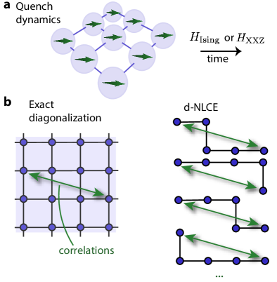
In this paper, we demonstrate a numerical linked cluster expansion method for calculating dynamics (d-NLCE). We show that it dramatically outperforms ED for calculating the short-to-moderate time spin-model dynamics that is common to many ultracold experiments van den Worm et al. (2013); Yan et al. (2013); Hazzard et al. (2014, 2013); Wall et al. (2015); de Paz et al. (2013, 2016); Lepoutre et al. (2017); Bohnet et al. (2016); Garttner et al. (2017); Richerme et al. (2014); Zhang et al. (2017); Jurcevic et al. (2014); Zeiher et al. (2016); Piñeiro Orioli et al. (2017); Takei et al. (2016); Nipper et al. (2012); Jau et al. (2016); Bernien et al. (2017); Greif et al. (2015); Brown et al. (2015); Kanász-Nagy et al. (2017); Carlström et al. (2016); Heidrich-Meisner et al. (2009); White et al. (2016); Gluza et al. (2016), illustrated in Fig. 1(a). It achieves these results with a significantly reduced computational cost.
As we will see, d-NLCE reduces to performing ED on a number of sub-clusters of the full lattice. Remarkably, it often yields accurate results including only a handful of small site clusters. d-NLCE results for sites are often substantially more accurate than ED with as many as – sites. This difference in is more striking when recast in terms of the computational cost of the algorithms, since this cost scales exponentially with : d-NLCE is frequently more accurate than ED calculations that require – more computational time and memory for the spin-1/2 models that we consider in this paper. This advantage is expected to be even larger for fermionic or bosonic lattice models, where the Hilbert space grows faster with .
NLCE.
NLCEs were introduced in Refs. Rigol et al. (2006, 2007a, 2007b) to calculate observables in equilibrium, as reviewed in Ref. Tang et al. (2013a). They have since been used to calculate equilibrium properties of numerous many-body systems Rigol and Singh (2009); Tang et al. (2015a); Khatami and Rigol (2011); Sahoo et al. (2016); Bruognolo et al. (2017); Benton (2017); Singh and Oitmaa (2012); Applegate et al. (2012); Hayre et al. (2013); Rigol and Singh (2007a, b); Khatami (2016); Khatami et al. (2015, 2014); Tang et al. (2012, 2013b); Khatami and Rigol (2012), including entanglement Sherman et al. (2016a); Hayward Sierens et al. (2017); Kallin et al. (2014); Stoudenmire et al. (2014); Kallin et al. (2013); Bruognolo et al. (2017) and spectra Sherman et al. (2016b), and to investigate many-body localization Tang et al. (2015b); Devakul and Singh (2015). More recently they have been used to calculate steady states after a quench Mallayya and Rigol (2017); Piroli et al. (2017); Rigol (2016); Iyer et al. (2015); Rigol (2014); Wouters et al. (2014) and in driven-dissipative systems Biella et al. (2017). In equilibrium, NLCEs are the methods of choice for ultracold fermionic atoms in optical lattices at strong interactions and current temperatures Cheuk et al. (2016); Khatami (2016); Duarte et al. (2015); Hart et al. (2015); Brown et al. (2017), complementing determinantal quantum Monte Carlo Blankenbecler et al. (1981) at weak interactions. Our work expands the NLCE method to dynamics, and shows that it is especially suitable to the types of dynamics that are now common in experiments in ultracold matter.
We now review the general algorithm for a linked cluster expansion, and describe d-NLCE in particular. All linked cluster expansions approximate an observable on a graph (such as a lattice) as a summation of this observable on finite connected (linked) clusters of sites. The relevant clusters may be any subset of the graph, including the full graph itself. Define as the expectation value of the observable for the system restricted to the cluster . Define the weight recursively as
| (1) |
where indexes every proper subcluster of , that is, every cluster whose components are contained in except itself 111There is considerable flexibility in defining which graphs constitute a cluster. From this it follows that
| (2) |
where indexes every subcluster of (including ). The significance of these definitions is that measures only the contribution to that arises due to correlations that span the cluster , that is, those where no site is uncorrelated from the rest. Thus only linked (i.e. contiguous) clusters need to be considered in Eq. (2), because any unlinked clusters have zero weight.
We approximate on the full lattice by truncating Eq. (2) to clusters up to size , giving
| (3) |
where indexes all the linked subclusters of the full lattice with number of sites less than or equal to . As , . This approximation converges rapidly as long as correlations decay sufficiently quickly with distance, since in this case approaches zero for sufficiently large clusters .
We see that linked cluster methods contain two steps. First, enumerate linked clusters up to a certain size (or some other criterion for truncation, such as number of bonds. In this paper, we always use number of sites). Although the computational cost of cluster enumeration grows combinatorically with size, this step has to be performed only once for a given lattice geometry (independent of the Hamiltonian). Second, solve for each cluster and use these to calculate . Since the clusters are diagonalized independently, NLCE can trivially utilize parallel computing architectures.
Perhaps the most familiar linked cluster method is a high-temperature series expansion (HTSE) Oitmaa et al. (2006), in which one enumerates all clusters with at most bonds and solves perturbatively to . NLCE replaces the perturbative solution with full diagonalization on each cluster. This is computationally more expensive for each cluster relative to HTSE, but improves the convergence properties for a given expansion order.
NLCE for dynamics.
Our d-NLCE method applies the NLCE to non-equilibrium systems using the same two steps described above: enumerate the clusters as we would in equilibrium, and calculate on each cluster using full diagonalization.
Figure 1 depicts the dynamics we consider, and suggests a qualitative advantage of d-NLCE over ED for this dynamics. The system begins in an initial product state where all spins are aligned in some direction. Then, it evolves under a transverse Ising or XXZ model, as shown in Fig. 1(a). The initial state is uncorrelated, but over time correlations grow between increasingly distant sites. To capture correlations between sites separated by with ED, one must use a system whose linear size is at least , as shown in Fig.1(b). This generically requires a number of sites where is the spatial dimension. In contrast, Fig. 1(c) shows how d-NLCE begins to capture these correlations as soon as one includes clusters with .
We compare d-NLCE with ED for dynamics governed by the transverse Ising and XXZ models,
| (4) | ||||
| (5) |
where , , and are spin-spin interactions, is the transverse field strength, is the Pauli matrix on site along direction , and indicates a summation over nearest neighbors. We consider the system to initially be in a uniform product state, . These two families of spin models are prototypical models in quantum statistical physics, and their dynamics initiated from such product states are being investigated in numerous ultracold experiments van den Worm et al. (2013); Yan et al. (2013); Hazzard et al. (2014, 2013); Wall et al. (2015); de Paz et al. (2013, 2016); Lepoutre et al. (2017); Bohnet et al. (2016); Garttner et al. (2017); Richerme et al. (2014); Zhang et al. (2017); Jurcevic et al. (2014); Zeiher et al. (2016); Piñeiro Orioli et al. (2017); Takei et al. (2016); Nipper et al. (2012); Jau et al. (2016); Bernien et al. (2017).
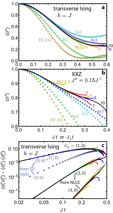
Figure 2 compares d-NLCE to ED with periodic boundary conditions for several cluster sizes. Throughout we choose an initial state with spins polarized along the direction, . Figures 2(a) and (b) show for the transverse Ising and XXZ models on a two-dimensional square lattice. These parameters are chosen to be representative. In both ED and d-NLCE, converges as is increased. In this way, both d-NLCE and ED monitor their own convergence by how closely successive results coincide with each other.
While both d-NLCE and ED converge, Fig. 2 shows that d-NLCE remains accurate to significantly longer times than ED, even when using somewhat smaller clusters. For example, for the transverse Ising results shown in Fig. 2(a), d-NLCE has visually converged for using site clusters. In contrast, ED shows clear discrepancies at times as short as , even while using significantly larger clusters with , which requires an exponentially greater computational cost. Even the d-NLCE is accurate to longer times than the ED. This trend also holds for the XXZ model: Fig. 2(b) shows that the d-NLCE converges for , while the more computationally demanding ED has noticeable discrepancies starting at .
d-NLCE also captures the growth of correlations in situations where ED fails severely. Figure 2(c) shows the dynamics of for sites and separated by , , and for the two-dimensional transverse Ising model. At short times, each of these grows polynomially with time. For each separation shown, d-NLCE captures this behavior exactly in any calculation with at least . In contrast, ED fails dramatically even when it uses a substantially larger . It predicts, for example, that the correlation is the same as the correlation (due to periodic boundary conditions), a result that is manifestly wrong and inaccurate by several orders of magnitude. As an aside, we note that while this leading order behavior can be captured by a short-time series expansion (STSE), the dynamical analog of the high temperature series expansion, the leading behavior of the correlations would require an STSE involving clusters with up to 10 bonds (up to 11 sites). In contrast, d-NLCE requires just .
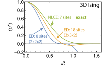
The d-NLCE method compares even more favorably with ED in three dimensions than in the two-dimensional models that we have just considered. As a particularly favorable example, Fig. 3 shows the Ising dynamics of on a cubic lattice. The d-NLCE reproduces the exact answer, which can be obtained analytically for this system Foss-Feig et al. (2013, 2013); Kastner (2011); Radin (1970), but ED is not accurate even on an site system. The minimum size required by ED to reproduce the exact result is in fact a site cluster with periodic boundaries, which requires – times more computational resources than d-NLCE 222This is a crude estimate: ED requires 20 additional sites, and hence a times larger Hilbert space. Matrix diagonalization scales as the cube of this, giving . However, d-NLCE requires a handful of clusters (though this is trivially parallelized) and accounting for symmetries decreases the ED Hilbert space, so a conservative factor of may be more appropriate.. We expect d-NLCE’s increased advantage over ED in three dimensions to hold quite generally. This is because, as illustrated in Fig. 1(b), clusters begin spanning the system’s correlation length at smaller .
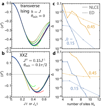
Finally, we plot the dynamics of in Figs. 4(a,b) for two cases with different initial conditions from Fig. 2. In these cases, both d-NLCE and ED appear to work well by visual inspection. In the transverse Ising model with these initial conditions, d-NLCE converges at most times shown for and for all times shown by , whereas ED has serious discrepancies at most times for and is visually converged for . For the XXZ model, all of the ED results shown appear to be accurate, while d-NLCE converges only around .
Although Figs. 4(a,b) indicate that ED provides comparable results to d-NLCE in some situations, in all the cases we study, d-NLCE converges more quickly as a function of cluster size. This is clearly shown in Figs. 4(c,d), where we plot the difference between results at two consecutive 333We calculate ED results at and . For other , we interpolate these results to determine the s (at a fixed time), as a function of . Both methods converge roughly exponentially. However, d-NLCE converges exponentially faster, i.e. d-NLCE provides a greater increase in accuracy for each increase in , in accord with the intuition presented in Fig. 1(b). The d-NLCE’s becomes smaller than that of ED for between 5 and 10.
Conclusions.
We have developed a numerical linked cluster expansion for out-of-equilibrium quantum dynamics and demonstrated that it is able to accurately capture dynamics relevant to numerous ongoing experiments in ultracold matter. We compared d-NLCE against ED, often the best previously available method, and found that d-NLCE (i) converges to longer times while utilizing the same number of sites, (ii) converges more quickly as a function of the cluster size, and (iii) captures leading-order evolution of correlations with a drastically reduced cluster size. The reduced cluster sizes required result in exponentially faster computation. The advantages of d-NLCE were clear in two-dimensions, and even larger in three dimensions. They are expected to be more pronounced for systems with larger on-site Hilbert spaces, like large spins or Fermi-Hubbard models, where the Hilbert space dimension grows even faster with cluster size, compounding d-NLCE’s advantage of utilizing smaller clusters than ED for a given level of accuracy.
The basic d-NLCE method used here can be improved and optimized in several ways. Although we sum all clusters up to a maximum size, choosing different sets of clusters can improve accuracy. Furthermore, equilibrium NLCE computations benefit from resummation techniques, and we expect that applying resummation to d-NLCE will improve its convergence as well, although different resummation techniques may be necessary out of equilibrium. Finally, calculations can be extended to higher order by improvements in the implementation: for example, numerically solving the cluster dynamics using Krylov subspace methods Schmitteckert (2004); García-Ripoll (2006), perhaps in combination with tensor network methods. d-NLCEs including clusters to or more sites are likely feasible with such improvements.
Acknowledgements.
This material is based upon work supported with funds from the Welch Foundation, grant no. C-1872. KRAH thanks the Aspen Center for Physics, which is supported by the National Science Foundation grant PHY-1066293, for its hospitality while part of this work was performed.References
- Polkovnikov et al. (2011) A. Polkovnikov, K. Sengupta, A. Silva, and M. Vengalattore, Rev. Mod. Phys. 83, 863 (2011).
- Lamacraft and Moore (2012) A. Lamacraft and J. Moore, in Ultracold Bosonic and Fermionic Gases, Volume 5 (Contemporary Concepts of Condensed Matter Science) (Elsevier, Oxford, UK, 2012).
- Langen et al. (2015) T. Langen, R. Geiger, and J. Schmiedmayer, Ann. Rev. Cond. Mat. Phys. 6, 201 (2015).
- Altman (2015) E. Altman, ArXiv e-prints (2015), arXiv:1512.00870 [cond-mat.quant-gas] .
- Basov et al. (2011) D. N. Basov, R. D. Averitt, D. van der Marel, M. Dressel, and K. Haule, Rev. Mod. Phys. 83, 471 (2011).
- Nicoletti and Cavalleri (2016) D. Nicoletti and A. Cavalleri, Adv. Opt. Photon. 8, 401 (2016).
- Giannetti et al. (2016) C. Giannetti, M. Capone, D. Fausti, M. Fabrizio, F. Parmigiani, and D. Mihailovic, Adv. Phys. 65, 58 (2016).
- Bray (1994) A. J. Bray, Adv. Phys. 43, 357 (1994).
- Calabrese and Gambassi (2005) P. Calabrese and A. Gambassi, J. Phys. A: Math. Gen. 38, R133 (2005).
- Henkel and Pleimling (2010) M. Henkel and M. Pleimling, Non-Equilibrium Phase Transitions: Volume 2: Ageing and Dynamical Scaling Far from Equilibrium (Springer, Netherlands, 2010).
- Henkel et al. (2009) M. Henkel, H. Hinrichsen, and S. Lübeck, Non-Equilibrium Phase Transitions: Volume 1: Absorbing Phase Transitions (Springer, Netherlands, 2009).
- Kamenev (2011) A. Kamenev, Field theory of Non-equilibrium systems (Cambridge University Press, Cambridge, 2011).
- Täuber (2014) U. C. Täuber, Critical dynamics: a field theory approach to equilibrium and non-equilibrium scaling behavior (Cambridge University Press, Cambridge, 2014).
- Walls and Milburn (1994) D. F. Walls and G. J. Milburn, Quantum Optics (Springer, 1994).
- Polkovnikov (2003) A. Polkovnikov, Phys. Rev. A 68, 053604 (2003).
- Blakie† et al. (2008) P. Blakie†, A. Bradley†, M. Davis, R. Ballagh, and C. Gardiner, Adv. Phys. 57, 363 (2008).
- Gardiner and Zoller (2004) C. Gardiner and P. Zoller, Quantum Noise (Springer-Verlag, 2004).
- Polkovnikov (2010) A. Polkovnikov, Ann. Phys. 325, 1790 (2010).
- Schachenmayer et al. (2015a) J. Schachenmayer, A. Pikovski, and A. M. Rey, Phys. Rev. X 5, 011022 (2015a).
- Schachenmayer et al. (2015b) J. Schachenmayer, A. Pikovski, and A. M. Rey, New J. Phys. 17, 065009 (2015b).
- Pucci et al. (2016) L. Pucci, A. Roy, and M. Kastner, Phys. Rev. B 93, 174302 (2016).
- Piñeiro Orioli et al. (2017) A. Piñeiro Orioli, A. Safavi-Naini, M. L. Wall, and A. M. Rey, Phys. Rev. A 96, 033607 (2017).
- Schollwöck (2011) U. Schollwöck, Ann. Phys. 326, 96 (2011).
- Sandvik (2010) A. W. Sandvik, AIP Conference Proceedings 1297, 135 (2010).
- van den Worm et al. (2013) M. van den Worm, B. C. Sawyer, J. J. Bollinger, and M. Kastner, New J. Phys. 15, 083007 (2013).
- Yan et al. (2013) B. Yan, S. A. Moses, B. Gadway, J. P. Covey, K. R. A. Hazzard, A. M. Rey, D. S. Jin, and J. Ye, Nature 501, 521 (2013).
- Hazzard et al. (2014) K. R. A. Hazzard, B. Gadway, M. Foss-Feig, B. Yan, S. A. Moses, J. P. Covey, N. Y. Yao, M. D. Lukin, J. Ye, D. S. Jin, and A. M. Rey, Phys. Rev. Lett. 113, 195302 (2014).
- Hazzard et al. (2013) K. R. A. Hazzard, S. R. Manmana, M. Foss-Feig, and A. M. Rey, Phys. Rev. Lett. 110, 075301 (2013).
- Wall et al. (2015) M. L. Wall, K. R. A. Hazzard, and A. M. Rey, in From atomic to mesoscale: The Role of Quantum Coherence in Systems of Various Complexities, edited by S. Malinovskaya and I. Novikova (World Scientific, Singapore, 2015) Chap. 1.
- de Paz et al. (2013) A. de Paz, A. Sharma, A. Chotia, E. Maréchal, J. H. Huckans, P. Pedri, L. Santos, O. Gorceix, L. Vernac, and B. Laburthe-Tolra, Phys. Rev. Lett. 111, 185305 (2013).
- de Paz et al. (2016) A. de Paz, P. Pedri, A. Sharma, M. Efremov, B. Naylor, O. Gorceix, E. Maréchal, L. Vernac, and B. Laburthe-Tolra, Phys. Rev. A 93, 021603 (2016).
- Lepoutre et al. (2017) S. Lepoutre, K. Kechadi, B. Naylor, B. Zhu, L. Gabardos, L. Isaev, P. Pedri, A. M. Rey, L. Vernac, and B. Laburthe-Tolra, ArXiv e-prints (2017), arXiv:1705.08358 [cond-mat.quant-gas] .
- Bohnet et al. (2016) J. G. Bohnet, B. C. Sawyer, J. W. Britton, M. L. Wall, A. M. Rey, M. Foss-Feig, and J. J. Bollinger, Science 352, 1297 (2016).
- Garttner et al. (2017) M. Garttner, J. G. Bohnet, A. Safavi-Naini, M. L. Wall, J. J. Bollinger, and A. M. Rey, Nat. Phys. 13, 781 (2017).
- Richerme et al. (2014) P. Richerme, Z.-X. Gong, A. Lee, C. Senko, J. Smith, M. Foss-Feig, S. Michalakis, A. V. Gorshkov, and C. Monroe, Nature 511, 198 (2014).
- Zhang et al. (2017) J. Zhang, G. Pagano, P. W. Hess, A. Kyprianidis, P. Becker, H. Kaplan, A. V. Gorshkov, Z.-X. Gong, and C. Monroe, ArXiv e-prints (2017), arXiv:1708.01044 [quant-ph] .
- Jurcevic et al. (2014) P. Jurcevic, B. P. Lanyon, P. Hauke, C. Hempel, P. Zoller, R. Blatt, and C. F. Roos, Nature 511, 202 (2014).
- Zeiher et al. (2016) J. Zeiher, R. van Bijnen, P. Schausz, S. Hild, J.-y. Choi, T. Pohl, I. Bloch, and C. Gross, Nat. Phys. 12, 1095 (2016).
- Piñeiro Orioli et al. (2017) A. Piñeiro Orioli, A. Signoles, H. Wildhagen, G. Günter, J. Berges, S. Whitlock, and M. Weidemüller, ArXiv e-prints (2017), arXiv:1703.05957 [physics.atom-ph] .
- Takei et al. (2016) N. Takei, C. Sommer, C. Genes, G. Pupillo, H. Goto, K. Koyasu, H. Chiba, M. Weidemüller, and K. Ohmori, Nat. Commun. 7, 13449 (2016).
- Nipper et al. (2012) J. Nipper, J. B. Balewski, A. T. Krupp, B. Butscher, R. Löw, and T. Pfau, Phys. Rev. Lett. 108, 113001 (2012).
- Jau et al. (2016) Y.-Y. Jau, A. M. Hankin, T. Keating, I. H. Deutsch, and G. W. Biedermann, Nat. Phys. 12, 71 (2016).
- Bernien et al. (2017) H. Bernien, S. Schwartz, A. Keesling, H. Levine, A. Omran, H. Pichler, S. Choi, A. S. Zibrov, M. Endres, M. Greiner, V. Vuletić, and M. D. Lukin, ArXiv e-prints (2017), arXiv:1707.04344 [quant-ph] .
- Greif et al. (2015) D. Greif, G. Jotzu, M. Messer, R. Desbuquois, and T. Esslinger, Phys. Rev. Lett. 115, 260401 (2015).
- Brown et al. (2015) R. C. Brown, R. Wyllie, S. B. Koller, E. A. Goldschmidt, M. Foss-Feig, and J. Porto, Science 348, 540 (2015).
- Kanász-Nagy et al. (2017) M. Kanász-Nagy, I. Lovas, F. Grusdt, D. Greif, M. Greiner, and E. A. Demler, Phys. Rev. B 96, 014303 (2017).
- Carlström et al. (2016) J. Carlström, N. Prokof’ev, and B. Svistunov, Phys. Rev. Lett. 116, 247202 (2016).
- Heidrich-Meisner et al. (2009) F. Heidrich-Meisner, S. R. Manmana, M. Rigol, A. Muramatsu, A. E. Feiguin, and E. Dagotto, Phys. Rev. A 80, 041603 (2009).
- White et al. (2016) I. G. White, R. G. Hulet, and K. R. A. Hazzard, ArXiv e-prints (2016), arXiv:1612.05671 [cond-mat.quant-gas] .
- Gluza et al. (2016) M. Gluza, C. Krumnow, M. Friesdorf, C. Gogolin, and J. Eisert, Phys. Rev. Lett. 117, 190602 (2016).
- Rigol et al. (2006) M. Rigol, T. Bryant, and R. R. P. Singh, Phys. Rev. Lett. 97, 187202 (2006).
- Rigol et al. (2007a) M. Rigol, T. Bryant, and R. R. P. Singh, Phys. Rev. E 75, 061118 (2007a).
- Rigol et al. (2007b) M. Rigol, T. Bryant, and R. R. P. Singh, Phys. Rev. E 75, 061119 (2007b).
- Tang et al. (2013a) B. Tang, E. Khatami, and M. Rigol, Comput. Phys. Commun. 184, 557 (2013a).
- Rigol and Singh (2009) M. Rigol and R. R. Singh, Comput. Phys. Commun. 180, 540 (2009).
- Tang et al. (2015a) B. Tang, D. Iyer, and M. Rigol, Phys. Rev. B 91, 174413 (2015a).
- Khatami and Rigol (2011) E. Khatami and M. Rigol, Phys. Rev. B 83, 134431 (2011).
- Sahoo et al. (2016) S. Sahoo, E. M. Stoudenmire, J.-M. Stéphan, T. Devakul, R. R. P. Singh, and R. G. Melko, Phys. Rev. B 93, 085120 (2016).
- Bruognolo et al. (2017) B. Bruognolo, Z. Zhu, S. R. White, and E. Miles Stoudenmire, ArXiv e-prints (2017), arXiv:1705.05578 [cond-mat.str-el] .
- Benton (2017) O. Benton, ArXiv e-prints (2017), arXiv:1706.09238 [cond-mat.str-el] .
- Singh and Oitmaa (2012) R. R. P. Singh and J. Oitmaa, Phys. Rev. B 85, 144414 (2012).
- Applegate et al. (2012) R. Applegate, N. R. Hayre, R. R. P. Singh, T. Lin, A. G. R. Day, and M. J. P. Gingras, Phys. Rev. Lett. 109, 097205 (2012).
- Hayre et al. (2013) N. R. Hayre, K. A. Ross, R. Applegate, T. Lin, R. R. P. Singh, B. D. Gaulin, and M. J. P. Gingras, Phys. Rev. B 87, 184423 (2013).
- Rigol and Singh (2007a) M. Rigol and R. R. P. Singh, Phys. Rev. Lett. 98, 207204 (2007a).
- Rigol and Singh (2007b) M. Rigol and R. R. P. Singh, Phys. Rev. B 76, 184403 (2007b).
- Khatami (2016) E. Khatami, Phys. Rev. B 94, 125114 (2016).
- Khatami et al. (2015) E. Khatami, R. T. Scalettar, and R. R. P. Singh, Phys. Rev. B 91, 241107 (2015).
- Khatami et al. (2014) E. Khatami, E. Perepelitsky, M. Rigol, and B. S. Shastry, Phys. Rev. E 89, 063301 (2014).
- Tang et al. (2012) B. Tang, T. Paiva, E. Khatami, and M. Rigol, Phys. Rev. Lett. 109, 205301 (2012).
- Tang et al. (2013b) B. Tang, T. Paiva, E. Khatami, and M. Rigol, Phys. Rev. B 88, 125127 (2013b).
- Khatami and Rigol (2012) E. Khatami and M. Rigol, Phys. Rev. A 86, 023633 (2012).
- Sherman et al. (2016a) N. E. Sherman, T. Devakul, M. B. Hastings, and R. R. P. Singh, Phys. Rev. E 93, 022128 (2016a).
- Hayward Sierens et al. (2017) L. E. Hayward Sierens, P. Bueno, R. R. P. Singh, R. C. Myers, and R. G. Melko, Phys. Rev. B 96, 035117 (2017).
- Kallin et al. (2014) A. B. Kallin, E. M. Stoudenmire, P. Fendley, R. R. P. Singh, and R. G. Melko, J. Stat. Mech. 2014, P06009 (2014).
- Stoudenmire et al. (2014) E. M. Stoudenmire, P. Gustainis, R. Johal, S. Wessel, and R. G. Melko, Phys. Rev. B 90, 235106 (2014).
- Kallin et al. (2013) A. B. Kallin, K. Hyatt, R. R. P. Singh, and R. G. Melko, Phys. Rev. Lett. 110, 135702 (2013).
- Sherman et al. (2016b) N. E. Sherman, T. Imai, and R. R. P. Singh, Phys. Rev. B 94, 140415 (2016b).
- Tang et al. (2015b) B. Tang, D. Iyer, and M. Rigol, Phys. Rev. B 91, 161109 (2015b).
- Devakul and Singh (2015) T. Devakul and R. R. P. Singh, Phys. Rev. Lett. 115, 187201 (2015).
- Mallayya and Rigol (2017) K. Mallayya and M. Rigol, Phys. Rev. E 95, 033302 (2017).
- Piroli et al. (2017) L. Piroli, E. Vernier, P. Calabrese, and M. Rigol, Phys. Rev. B 95, 054308 (2017).
- Rigol (2016) M. Rigol, Phys. Rev. Lett. 116, 100601 (2016).
- Iyer et al. (2015) D. Iyer, M. Srednicki, and M. Rigol, Phys. Rev. E 91, 062142 (2015).
- Rigol (2014) M. Rigol, Phys. Rev. Lett. 112, 170601 (2014).
- Wouters et al. (2014) B. Wouters, J. De Nardis, M. Brockmann, D. Fioretto, M. Rigol, and J.-S. Caux, Phys. Rev. Lett. 113, 117202 (2014).
- Biella et al. (2017) A. Biella, J. Jin, O. Viyuela, C. Ciuti, R. Fazio, and D. Rossini, ArXiv e-prints (2017), arXiv:1708.08666 [cond-mat.stat-mech] .
- Cheuk et al. (2016) L. W. Cheuk, M. A. Nichols, K. R. Lawrence, M. Okan, H. Zhang, E. Khatami, N. Trivedi, T. Paiva, M. Rigol, and M. W. Zwierlein, Science 353, 1260 (2016).
- Duarte et al. (2015) P. M. Duarte, R. A. Hart, T.-L. Yang, X. Liu, T. Paiva, E. Khatami, R. T. Scalettar, N. Trivedi, and R. G. Hulet, Phys. Rev. Lett. 114, 070403 (2015).
- Hart et al. (2015) R. A. Hart, P. M. Duarte, T.-L. Yang, X. Liu, T. Paiva, E. Khatami, R. T. Scalettar, N. Trivedi, D. A. Huse, and R. G. Hulet, Nature 519, 211 (2015).
- Brown et al. (2017) P. T. Brown, D. Mitra, E. Guardado-Sanchez, P. Schauß, S. S. Kondov, E. Khatami, T. Paiva, N. Trivedi, D. A. Huse, and W. S. Bakr, Science 357, 1385 (2017).
- Blankenbecler et al. (1981) R. Blankenbecler, D. J. Scalapino, and R. L. Sugar, Phys. Rev. D 24, 2278 (1981).
- Note (1) There is considerable flexibility in defining which graphs constitute a cluster.
- Oitmaa et al. (2006) J. Oitmaa, C. Hamer, and W. Zheng, Series Expansion Methods for Strongly Interacting Lattice Models (Cambridge, 2006).
- Foss-Feig et al. (2013) M. Foss-Feig, K. R. A. Hazzard, J. J. Bollinger, and A. M. Rey, Phys. Rev. A 87, 042101 (2013).
- Foss-Feig et al. (2013) M. Foss-Feig, K. R. A. Hazzard, J. J. Bollinger, A. M. Rey, and C. W. Clark, New J. Phys. 15, 113008 (2013).
- Kastner (2011) M. Kastner, Phys. Rev. Lett. 106, 130601 (2011).
- Radin (1970) C. Radin, J. Math. Phys. 11, 2945 (1970), http://dx.doi.org/10.1063/1.1665079 .
- Note (2) This is a crude estimate: ED requires 20 additional sites, and hence a times larger Hilbert space. Matrix diagonalization scales as the cube of this, giving . However, d-NLCE requires a handful of clusters (though this is trivially parallelized) and accounting for symmetries decreases the ED Hilbert space, so a conservative factor of may be more appropriate.
- Note (3) We calculate ED results at and . For other , we interpolate these results to determine the s.
- Schmitteckert (2004) P. Schmitteckert, Phys. Rev. B 70, 121302 (2004).
- García-Ripoll (2006) J. J. García-Ripoll, New J. Phys. 8, 305 (2006).