Zero Variance and Hamiltonian Monte Carlo Methods in GARCH Models

Abstract

In this paper, we develop Bayesian Hamiltonian Monte Carlo methods for inference in asymmetric GARCH models under different distributions for the error term. We implemented Zero-variance and Hamiltonian Monte Carlo schemes for parameter estimation to try and reduce the standard errors of the estimates thus obtaing more efficient results at the price of a small extra computational cost.

Key words: GARCH, Bayesian approach, zero variance MCMC, Hamiltonian Monte Carlo.

1 Introduction

ARCH and GARCH models first introduced by Engle (1982) and generalized by Bollerslev (1986) is certainly the most used class of models to study the volatility of financial markets and have been around for decades now (see for example Teräsvirta (2009) and Tsay (2010)). In terms of the statistical framework, these models provide motion dynamics for the dependency in the conditional time variation of the distributional parameters of the mean and variance, in an attempt to capture such phenomena as autocorrelation in returns and squared returns. Extensions to these models have included more sophisticated dynamics such as threshold models to capture the asymmetry in the news impact. An example is the extended version of the GARCH model proposed in Glosten et al. (1993) (GJR-GARCH hereafter). This composite model deals with possible asymmetries in the volatility responses incorporating a leverage effect in the volatility equation.

From a Bayesian perspective, computational methods based on Markov chain Monte Carlo (MCMC) have been utilized to address the complexity of these models. These are considered one of the most efficient estimation methods for this class of models. For a survey on Bayesian estimation of GARCH models see for example Virbickaitė et al. (2015).

Zero-variance MCMC methods using control variates can dramatically reduce the Monte Carlo variance of Bayesian estimates based on the posterior expectation. Recently, Mira et al. (2013) showed how ZV-MCMC can be applied to estimate the parameters in a univariate GARCH(1,1) model with Gaussian errors. Many empirical studies however, indicate that this model does not account for the degree of kurtosis usually observed in most financial time series. It is also known that the distribution of asset returns exhibit the so called leverage effect, i.e. a negative past return tends to increase the present volatility. In this paper we discuss the use and efficiency of zero-variance MCMC (ZV-MCMC) coupled with Hamiltonian Monte Carlo (HMC) methods to estimate GJR-GARCH models. To increase flexibility we allow the error terms to follow normal, $t$-Student, Generalized Error Distribution (GED) and the Generalized $t$ (GT) distributions (McDonald and Newey (1988)) with mean zero and unit variance.

The main contributions of the paper are to provide closed-form analytic expressions necessary to implement the methods and assess their statistical performances via simulation studies. We also illustrate with real time series data. To our knowledge, such methods have not been applied and studied before in the context of GJR-GARCH models. All the computations in this paper were implemented using the C++ programming language through the Rcpp and RcppArmadillo which are available in the open-source statistical software language and environment R (R Development Core Team (2015)).

The remainder of the paper is organized as follows. Section 2 describes the Bayesian model and the associated algorithms used for inference. In Section 3 a simulation study is conducted to illustrate the flexibity and computational gains in using the proposed algorithms. Section 4 presents a financial application using index data and Section 5 concludes the paper.

2 Methodology

The so called GJR-GARCH model (Glosten et al. (1993)) is widely used to describe leverage effects as it takes into account possible asymmetries in individual assets volatilities. The model is defined as,

$$x_{y} = y_{y}+\mu$$

$$y_{t} = \epsilon_{t}\sqrt{h_{t}}~{},~{}\epsilon_{t}\sim D(0,1)$$

$$h_{t} = \omega+\sum_{i=1}^{p}(\alpha_{i}+\phi_{i}I_{t-i})y_{t-i}^{2}+\sum_{j=1}^{q}\beta_{j}h_{t-j},$$

where the $\epsilon_{t}$ are independent and identically distributed error terms and $D(0,1)$ denotes a distribution with mean zero and variance 1. Then, given the past history at time $t$ denoted $F_{t-1}=\{y_{t-1},y_{t-2},\dots\}$, $h_{t}$ is the conditional variance of $y_{t}$ written as an exact function of the past. Also, $\omega>0$, $\alpha_{i}+\phi_{i}\geq 0,i=1,\dots,p$ and $\beta_{j}\geq 0,j=1,\dots,q$ define the positivity constraints and $\sum_{i=1}^{p}(\alpha_{i}+\phi_{i}/2)+\sum_{j=1}^{q}\beta_{j}<1$, ensures covariance stationarity of $h_{t}$. In the variance equation, the indicator function $I_{t-i}=1$ if $y_{t-i}\leq 0$ and $I_{t-i}=0$ otherwise clearly induces a possibly asymmetric effect of $y_{t-i}^{2}$ on $h_{t}$. Finally, it is clear that if $\phi_{i}=0,i=1,\dots,p$ this model reduces to the GARCH($p,q$) model with symmetric effects.

2.1 Likelihood and Prior Distributions

Following the Bayesian paradigm we need to complete the model specification with appropriate prior distributions for the parameters. The likelihood function,

$$f(y_{t}|h_{t},\nu)=h_{t}^{-1/2}\frac{1}{\sqrt{\pi(\nu-2)}}\frac{\Gamma(\frac{\nu+1}{2})}{\Gamma(\frac{\nu}{2})}\left\{1+\frac{y_{t}^{2}}{(\nu-2)h_{t}}\right\}^{-(\nu+1)/2}$$

for $t$-Student errors with degrees of freedom parameter $\nu>2$ and,

$$f(y_{t}|h_{t},\nu)=h_{t}^{-1/2}\frac{\nu}{\lambda 2^{1+1/\nu}\Gamma(1/\nu)}\exp\left\{-\frac{1}{2\lambda^{\nu}}\left|\frac{y_{t}}{\sqrt{h_{t}}}\right|^{\nu}\right\}$$

for GED errors with shape parameter $\nu>0$ where $\lambda^{2}=2^{-2/\nu}\Gamma(1/\nu)/\Gamma(3/\nu)$. Since its kurtosis is given by $\Gamma(1/\nu)\Gamma(5/\nu)/\Gamma(3/\nu)^{2}-3$ then when $0<\nu<2$ this distribution reproduces heavy-tails. Also, two special cases of the GED are the standard normal distribution when $\nu=2$ and the Laplace (or double exponential) distribution for $\nu=1$.

Finally, for the generalized $t$ errors,

$$f(y_{t}|h_{t},\eta,\nu)=h_{t}^{-1/2}\frac{\eta\Gamma\left(\nu+\frac{1}{\eta}\right)}{2\nu^{1/\eta}\Gamma\left(\frac{1}{\eta}\right)\Gamma\left(\nu\right)}\left(1+\frac{1}{\nu}\left|\frac{x}{\sqrt{h_{t}}}\right|^{\eta}\right)^{-(\nu+1/\eta)},$$

where $\eta>0$ and $\nu>0$ are two shape parameters. Larger values of $\eta$ and $\nu$ yield a density with thinner tails than the normal while smaller values are associated with thicker tailed densities.

We propose the following prior distributions for the tail parameter $\nu$. For GED errors, $\nu\sim N(0,\sigma^{2}_{\nu})$ truncated to $\nu>0$ while for Student-$t$ errors we consider a $N(0,\sigma^{2}_{\nu})$ distribution truncated to $\nu>2$. For GT errors, $\eta\sim N(0,\sigma^{2}_{\eta})$ truncated to $\eta>1$ and $\nu\sim N(0,\sigma^{2}_{\nu})$ truncated to $\nu>1/\eta$. For the parameters in the variance equation we also assign truncated normal prior distributions, $\omega\sim N(0,\sigma^{2}_{\omega})$ truncated to $\omega>0$, $\alpha\sim N(0,\sigma^{2}_{\alpha})$ truncated to $0<\alpha<1$, $\beta\sim N(0,\sigma^{2}_{\beta})$ truncated to $0<\beta<1$, $\phi\sim N(0,\sigma^{2}_{\phi})$ truncated to $0<\phi<2$. Finally, we assign a normal distribution for mean parameter, $\mu\sim N(0,\sigma^{2}_{\mu})$.

Also, in order to employ the algorithms in this paper we need to implement transformations of model parameters to the real line. Here we propose to the following set of parametric transformations, $\omega^{\ast}=\log(\omega)$, $\alpha^{\ast}=\log\left(\frac{\alpha}{1-\alpha}\right)$, $\phi^{\ast}=\log\left(\frac{2\phi}{1-\phi}\right)$, $\beta^{\ast}=\log\left(\frac{\beta}{1-\beta}\right)$. For the parameters in the error distribution we take $\nu^{\ast}=\log(\nu+c)$ and $\eta^{\ast}=\log(\eta)$ where $c$ is the model constraint.

2.2 Zero Variance Methods

We assume that the aim is to estimate the expected value of a function $f$ of the parameters $\theta$ with respect to their (unnormalized) posterior distribution $\pi$, i.e.

$$\mu_{f}=E_{\pi}[f(\hbox{\boldmath$\theta$})]=\frac{\displaystyle\int f(\hbox{\boldmath$\theta$})\pi(\hbox{\boldmath$\theta$})d\hbox{\boldmath$\theta$}}{\displaystyle\int\pi(\hbox{\boldmath$\theta$})d\hbox{\boldmath$\theta$}}.$$

Now, given a sample of size $N$, $\hbox{\boldmath$\theta$}^{(1)},\dots,\hbox{\boldmath$\theta$}^{(N)}$, from the posterior distribution, $\mu_{f}$ is estimated as $\hat{\mu}_{f}=\sum_{i=1}^{N}f(\hbox{\boldmath$\theta$}^{(i)})/N$. In order to reduce the Monte Carlo error of this estimate the idea is to replace $f$ by a function $\tilde{f}$ which is constructed such that $E_{\pi}(\tilde{f})=\mu_{f}$ but its variance is much smaller. The zero-variance (ZV) principle was introduced in the physics literature by Assaraf and Caffarel (1999) and Assaraf and Caffarel (2003) and latter studied in Mira et al. (2013) where rigorous conditions for unbiasedness and existence of a central limit theorem (CLT) were derived. In what follows, we use the re-normalized function $\tilde{f}$ defined as,

$$\tilde{f}(\hbox{\boldmath$\theta$})=f(\hbox{\boldmath$\theta$})+\frac{H\psi}{\sqrt{\pi(\hbox{\boldmath$\theta$})}}$$ (1)

where $H$ is a Hamiltonian operator and $\psi$ is an arbitrary trial function. If Equation (1) satisfies $\mu_{f}=\mu_{\tilde{f}}$ then $\tilde{f}$ can also be used to estimate the desired quantity given a sample from the posterior distribution. So, in practice this condition must be verified as it depends on the choices of $H$ and $\psi$. Defining $\sigma_{f}$ as the standard deviation of $f$ with respect to $\pi$, the optimal choice of $H$ and $\psi$ is obtained by setting $\sigma_{\tilde{f}}=0$ (or equivalently $\tilde{f}=\mu_{f}$) which in turn leads to the following fundamental equation,

$$H\psi=-\sqrt{\pi(\hbox{\boldmath$\theta$})}[f(\hbox{\boldmath$\theta$})-\mu_{f}].$$

Unfortunately, in most practical applications this cannot be solved analytically and an approximate solution is proposed in Mira et al. (2013) as follows. First specify the operator $H$ which is required to be Hermitian and satisfy $H\sqrt{\pi}=0$. Then, parameterize $\psi$ in terms of optimal parameters by minimizing $\sigma_{\tilde{f}}$ and estimate these parameters from a short MCMC simulation. Finally, a long MCMC simulation is performed from which the posterior expectation is approximated using $\hat{\mu}_{\tilde{f}}$ instead of $\hat{\mu}_{f}$. Here we adopt the so called Schrödinger-type Hamiltonian operator proposed in Assaraf and Caffarel (1999). For $\hbox{\boldmath$\theta$}\in\mathbb{R}^{d}$,

$$H(\hbox{\boldmath$\theta$})=-\frac{1}{2}\sum_{j=1}^{d}\frac{\partial^{2}}{\partial\theta_{i}^{2}}+V(\hbox{\boldmath$\theta$})$$ (2)

where $V(\hbox{\boldmath$\theta$})=\frac{1}{2\sqrt{\pi({\scriptsize\hbox{\boldmath$\theta$}})}}\Delta_{{\scriptsize\hbox{\boldmath$\theta$}}}\sqrt{\pi(\hbox{\boldmath$\theta$})}$ and $\Delta_{{\scriptsize\hbox{\boldmath$\theta$}}}$ denotes the Laplace operator of second derivatives $\sum_{i=1}^{d}\frac{\partial^{2}}{\partial\theta_{i}^{2}}$. This choice of operator guarantees the necessary condition $H\sqrt{\pi}=0$.

The trial function $\psi$ is typically chosen as $\psi(\hbox{\boldmath$\theta$})=P(\hbox{\boldmath$\theta$})\sqrt{\pi(\hbox{\boldmath$\theta$})}$ where $P(\hbox{\boldmath$\theta$})$ is a polynomial function. In principle, a higher variance reduction can be achieved by simply using higher order polynomials. In practice however, it has been reported in the literature that first and second degree polynomials will provide considerable variance reduction (see Mira et al. (2013), Papamarkou et al. (2014) and Oates et al. (2016)).

This trial function is combined with the Hamiltonian in (2) giving rise to the following re-normalized function of $\theta$,

$$\tilde{f}(\hbox{\boldmath$\theta$})=f(\hbox{\boldmath$\theta$})-\frac{1}{2}\Delta_{{\scriptsize\hbox{\boldmath$\theta$}}}P(\hbox{\boldmath$\theta$})+\nabla_{{\scriptsize\hbox{\boldmath$\theta$}}}P(\hbox{\boldmath$\theta$})\hbox{\boldmath$z$}(\hbox{\boldmath$\theta$})$$

where $\hbox{\boldmath$z$}(\hbox{\boldmath$\theta$})=-\frac{1}{2}\nabla_{{\scriptsize\hbox{\boldmath$\theta$}}}\log\pi(\hbox{\boldmath$\theta$})$ and $\nabla_{{\scriptsize\hbox{\boldmath$\theta$}}}\log\pi(\hbox{\boldmath$\theta$})$ denotes the gradient vector of $\log\pi(\hbox{\boldmath$\theta$})$ with respect to $\theta$. The elements in $z$ are known as control variates. In particular, for a first degree polynomial, i.e $P(\hbox{\boldmath$\theta$})=\sum_{i=1}^{d}a_{i}\theta_{i}=\hbox{\boldmath$a$}^{\prime}\hbox{\boldmath$\theta$}$ it follows that $\tilde{f}(\hbox{\boldmath$\theta$})=f(\hbox{\boldmath$\theta$})+\hbox{\boldmath$a$}^{\prime}\hbox{\boldmath$z$}(\hbox{\boldmath$\theta$})$ and the coefficients $\hbox{\boldmath$a$}\in\mathbb{R}^{d}$ are chosen so as to minimize the variance of $\tilde{f}(\hbox{\boldmath$\theta$})$. It can be shown that these coefficients are given by,

$$\hbox{\boldmath$a$}=-Var[\hbox{\boldmath$z$}(\hbox{\boldmath$\theta$})]^{-1}Cov[f(\hbox{\boldmath$\theta$}),\hbox{\boldmath$z$}(\hbox{\boldmath$\theta$})]$$ (3)

and are estimated from a short MCMC simulation which generates a sample $\hbox{\boldmath$\theta$}^{(1)},\dots,\hbox{\boldmath$\theta$}^{(M)}$ from the posterior distribution. Substituting the matrices in (3) by the sample variance matrix of $\hbox{\boldmath$z$}(\hbox{\boldmath$\theta$}^{(l)})$ and the sample covariance matrix of $f(\hbox{\boldmath$\theta$}^{(l)})$ and $\hbox{\boldmath$z$}(\hbox{\boldmath$\theta$}^{(l)})$, $l=1,\dots,M$ we obtain an estimate $\hat{\hbox{\boldmath$a$}}$ of the coefficients. Once $\hat{\hbox{\boldmath$a$}}$ is computed we can proceed and perform a much longer simulation which generates a sample $\hbox{\boldmath$\theta$}^{(1)},\dots,\hbox{\boldmath$\theta$}^{(N)}$ from the posterior distribution of $\theta$. This gives rise to a sample of re-normalized functions,

$$\tilde{f}(\hbox{\boldmath$\theta$}^{(l)})=f(\hbox{\boldmath$\theta$}^{(l)})+\hat{\hbox{\boldmath$a$}}\hbox{\boldmath$z$}(\hbox{\boldmath$\theta$}^{(l)}),~{}l=1,\dots,N,$$

and the posterior expectation of $\theta$ is estimated as $\hat{\mu}_{\tilde{f}}=\sum_{l=1}^{N}\tilde{f}(\hbox{\boldmath$\theta$}^{(l)})/N$.

As was recently noticed by Papamarkou et al. (2014), these ZV methods can be embedded in sampling schemes that require the computation of gradients of the log-target density in the first place. This is the case for so called differential-geometric MCMC schemes like Hamiltonian Monte Carlo, Metropolis adjusted Langevin algorithm and their manifold extension (see Girolami and Calderhead (2011) for details).

2.3 Hamiltonian Monte Carlo

The random walk Metropolis-Hastings algorithm is a commonly used approach in the Bayesian literature for GARCH models. Hamiltonian Monte Carlo (HMC) methods on the other hand combine Gibbs updates with Metropolis updates and avoids the random walk behaviour which may lead to inefficient exploration of the parameter space. This method processes a new state by computing a trajectory obeying Hamiltonian dynamics (Neal (2011)).

Consider a random vector $\boldsymbol{\theta}\in\mathbb{R}^{k}$ as position variables (parameters) and $\hbox{\boldmath$r$}\in\mathbb{R}^{k}$ an independent auxiliary random vector with $\hbox{\boldmath$r$}\sim N_{k}(0,M)$. The parameter space in then augmented by this auxiliary parameter $r$ and the joint probability density function of $(\hbox{\boldmath$\theta$},\hbox{\boldmath$r$})$ is given by

$$\pi(\boldsymbol{\theta},\hbox{\boldmath$r$})\propto\exp(-H(\boldsymbol{\theta},\hbox{\boldmath$r$}))$$ (4)

where $H(\boldsymbol{\theta},\hbox{\boldmath$r$})=U(\boldsymbol{\theta})+K(\hbox{\boldmath$r$})$ is a Hamiltonian function, $U(\hbox{\boldmath$\theta$})=-\log[\pi(\hbox{\boldmath$\theta$}|y)\pi(\hbox{\boldmath$\theta$})]$ is refered to as the potential energy and $K(\hbox{\boldmath$r$})=\hbox{\boldmath$r$}^{\prime}M^{-1}\hbox{\boldmath$r$}/2$ is called the kinetic energy. A candidate value for $(\hbox{\boldmath$\theta$},bfr)$ is generated in two steps. First, a value of $r$ is simulated from a normal distribution with mean zero and covariance matrix $M$ independently of $\theta$. Second, the joint system $(\boldsymbol{\theta},\hbox{\boldmath$r$})$ made up of the current parameter value and the new momentum $r$ evolves through Hamiltonian dynamics defined by the pair of differential equations,

$$\frac{\partial\boldsymbol{\theta}}{\partial t}=\frac{H(\boldsymbol{\theta},\hbox{\boldmath$r$})}{\partial\hbox{\boldmath$r$}}=\frac{\partial K(\hbox{\boldmath$r$})}{\partial\hbox{\boldmath$r$}};\qquad\frac{\partial\hbox{\boldmath$r$}}{\partial t}=\frac{H(\boldsymbol{\theta},\hbox{\boldmath$r$})}{\partial\boldsymbol{\theta}}=-\frac{\partial U(\boldsymbol{\theta})}{\partial\boldsymbol{\theta}}.$$

In practice however, these equations cannot be solved analytically and must be discretized using some small stepsize $\epsilon>0$. The leapfrog operator is typically used to solve Hamilton’s equations (Leimkuhler and Reich (2004)) and works as follows,

$$r_{i}(t+\epsilon/2) = r_{i}(t)-(\epsilon/2)\frac{\partial U(\boldsymbol{\theta}(t))}{\partial\theta_{i}}$$

$$\theta_{i}(t+\epsilon) = \theta_{i}(t+\epsilon/2)-\epsilon\frac{\partial K(\hbox{\boldmath$r$}(t+\epsilon/2))}{\partial r_{i}}$$

$$r_{i}(t+\epsilon) = r_{i}(t+\epsilon/2)-(\epsilon/2)\frac{\partial U(\boldsymbol{\theta}(t+\epsilon))}{\partial\theta_{i}}$$

The resulting state at the end of $L$ repetitions of the above three steps is a proposal $(\hbox{\boldmath$\theta$}^{*},\hbox{\boldmath$r$}^{*})$ for the augmented parameter vector. Since this discretization introduces an error, a Metropolis acceptance probability is employed to correct this bias and ensure convergence to the invariant posterior distribution. The transition to a new proposed value is accepted with probability,

$$\mathbb{P}((\hbox{\boldmath$\theta$},\hbox{\boldmath$r$}),(\hbox{\boldmath$\theta$}^{*},\hbox{\boldmath$r$}^{*}))=\min\left\{1,\exp[H(\hbox{\boldmath$\theta$},\hbox{\boldmath$r$})-H(\hbox{\boldmath$\theta$}^{*},\hbox{\boldmath$r$}^{*})]\right\}$$

and otherwise rejected.

2.4 Influential Observations

In this section, we propose to compute the Kullback-Leibler (K-L) divergence to assess the potential influence of an observation in the posterior distribution (see for example Hao et al. (2016)). The idea is to compare the posterior density $p(\hbox{\boldmath$\theta$}|\hbox{\boldmath$y$})$ with a perturbed posterior density $p_{\delta}(\hbox{\boldmath$\theta$}|\hbox{\boldmath$y$})$ by measuring a divergence between $p(\hbox{\boldmath$\theta$}|\hbox{\boldmath$y$})$ and $p_{\delta}(\hbox{\boldmath$\theta$}|\hbox{\boldmath$y$})$. For a direct comparison, the Kullback-Leibler divergence between $p(\hbox{\boldmath$\theta$}|\hbox{\boldmath$y$})$ and $p_{\delta}(\hbox{\boldmath$\theta$}|\hbox{\boldmath$y$})$ is given by,

$$KL(p(\hbox{\boldmath$\theta$}|\hbox{\boldmath$y$}),p_{\delta}(\hbox{\boldmath$\theta$}|\hbox{\boldmath$y$}))=\int p(\hbox{\boldmath$\theta$}|\hbox{\boldmath$y$})\log\left(\frac{p(\hbox{\boldmath$\theta$}|\hbox{\boldmath$y$})}{p_{\delta}(\hbox{\boldmath$\theta$}|\hbox{\boldmath$y$})}\right)d\hbox{\boldmath$\theta$}.$$ (5)

We now define a general perturbation as the ratio of unnormalized posterior densities,

$$\delta(\hbox{\boldmath$\theta$},\hbox{\boldmath$y$}) = \frac{p_{\delta}(\hbox{\boldmath$y$}|\hbox{\boldmath$\theta$})p_{\delta}(\hbox{\boldmath$\theta$})}{p(\hbox{\boldmath$y$}|\hbox{\boldmath$\theta$})p(\hbox{\boldmath$\theta$})}$$ (6)

from which the perturbed posterior density can be written as,

$$p_{\delta}(\hbox{\boldmath$\theta$}|\hbox{\boldmath$y$})=\frac{\delta(\hbox{\boldmath$\theta$},\hbox{\boldmath$y$})p(\hbox{\boldmath$\theta$}|\hbox{\boldmath$y$})}{\int\delta(\hbox{\boldmath$\theta$},\hbox{\boldmath$y$})p(\hbox{\boldmath$\theta$}|\hbox{\boldmath$y$})d\hbox{\boldmath$\theta$}}.$$

So in terms of perturbation, the divergence (5) is written as,

$$KL(p(\hbox{\boldmath$\theta$}|\hbox{\boldmath$y$}),p_{\delta}(\hbox{\boldmath$\theta$}|\hbox{\boldmath$y$}))=\int p(\hbox{\boldmath$\theta$}|\hbox{\boldmath$y$})\log\left(\frac{\delta(\hbox{\boldmath$\theta$},\hbox{\boldmath$y$})}{\int\delta(\hbox{\boldmath$\theta$},\hbox{\boldmath$y$})p(\hbox{\boldmath$\theta$}|\hbox{\boldmath$y$})d\hbox{\boldmath$\theta$}}\right)^{-1}d\hbox{\boldmath$\theta$}.$$ (7)

In particular, to assess the potential influence of observations only the likelihood function is perturbed and the associated perturbation is given by,

$$\delta(\hbox{\boldmath$\theta$},\hbox{\boldmath$y$}) = \frac{p(\hbox{\boldmath$y$}_{(i)}|\hbox{\boldmath$\theta$})}{p(\hbox{\boldmath$y$}|\hbox{\boldmath$\theta$})}=\frac{\prod_{\stackrel{{\scriptstyle t=1}}{{t\neq i}}}^{n}p(y_{t}|F_{t-1},\hbox{\boldmath$\theta$})}{\prod_{t=1}^{n}p(y_{t}|F_{t-1},\hbox{\boldmath$\theta$})},$$ (8)

where $\hbox{\boldmath$y$}_{(i)}$ denotes the series with the $i$th observation deleted. In our GJR-GARCH(1,1) model however, for $t=i+1$ we need to redefine the conditional variance and consequently the $(i+1)$th term of the likelihood function in the numerator of (8). It is not difficult to verify that, $E(y_{i+1}|F_{i-1})=0$ and,

$$h_{i+1}=Var(y_{i+1}|F_{i-1}) = E(h_{i+1}\epsilon_{i+1}^{2}|F_{i-1})=E(h_{i+1}|F_{i-1})E(\epsilon_{i+1}^{2}|F_{i-1})$$

$$= E(h_{i+1}|F_{i-1})=\omega+[\alpha+\phi E(I_{i}|F_{i-1})]E(y_{i}^{2}|F_{i-1})+\beta h_{i}$$

$$= \omega+(\alpha+\phi/2+\beta)h_{i}$$

where we used the fact that $E(y_{i}^{2}|F_{i-1})=h_{i}$ and $E(I_{i}|F_{i-1})=P(I_{i}=1|F_{i-1})=1/2$ for symmetric distributions.

Then, given a sample $\hbox{\boldmath$\theta$}^{(1)},\dots,\hbox{\boldmath$\theta$}^{(N)}$ from the posterior distribution of $\theta$ we obtain the following approximation for the divergence of the $i$-th observation,

$$\widehat{KL}_{i}=\frac{1}{N}\sum_{l=1}^{N}\left[-\log\left(\frac{\delta_{i}(\hbox{\boldmath$\theta$}^{(l)},\hbox{\boldmath$y$})}{\bar{\delta}_{i}}\right)\right],~{}i=1,\dots,n.$$ (9)

where $\bar{\delta}_{i}=\frac{1}{N}\sum_{l=1}^{N}\delta_{i}(\hbox{\boldmath$\theta$}^{(l)},\hbox{\boldmath$y$})$ is the mean perturbation for the $i$-th observation.

Higher values of this positive valued measure provide indication for possibly influential observations. However, in a similar vein as suggested in Santos and Bolfarine (2016), we propose to analyse these quantities relatively to the others for each observation. This is accomplished by counting how many times each value is greater than the others along the MCMC simulations. So, given a sample from the posterior distribution we obtain samples of $KL$ divergences as,

$$KL_{i}^{(l)}=-\log\left(\frac{\delta_{i}(\hbox{\boldmath$\theta$}^{(l)},\hbox{\boldmath$y$})}{\bar{\delta}_{i}}\right),~{}i=1,\dots,n,~{}l=1,\dots,N$$

and for each $i$ we compute the following sample proportions,

$$P_{i}=\frac{1}{N}\sum_{l=1}^{N}I\left(KL_{i}^{(l)}>\max_{j\neq i}KL_{i}^{(l)}\right),~{}i=1,\dots,n.$$ (10)

Each of these proportions provides an estimate of the posterior probability of the $i$th observation being influential.

3 A Simulation Study

Here we concentrate on the performance of posterior means as parameter estimators using HMC methods as opposed to traditional MCMC (Random walk Metropolis) in the presence of variance reduction. We check the effect of relaxing the normal errors assumption and model misspecification.

To generate the artificial data we considered GJR-GARCH(1,1) models with four distributions for the errors: Gaussian, GED with parameter $\nu=0.8$, Student $t$ with $\nu=8$ degrees of freedom and generalized $t$ distribution with shape parameters $\nu=4$ and $\eta=1$. For each model we generated $m=200$ time series with $n=200,500,1000,2000$ observations and parameters $\omega=0.05$, $\alpha=0.05$, $\phi=0.1$, $\beta=0.85$ and $\mu=0$. So, the simulated returns induce possible asymmetric effects on the volatilities. Also, the persistence of the volatility processes, measured by $\alpha+\phi/2+\beta$ is 0.95 (a common finding when estimating such models). We assume independent truncated normal prior distributions are as described in Section 2.1 with large variances equal to 1000.

For the Metropolis-Hastings algorithm we proposed new parameter values from a multivariate normal distribution centered around the current value with a variance-covariance proposal matrix which was calculated from a pilot tunning procedure. Specifically, we construct a pilot sample of 2000 values from a Metropolis-Hastings with proposal variance-covariance matrix $\epsilon\hbox{\boldmath$I$}_{k}$. A sample variance-covariance matrix $M$ is then calculated from the output of this pilot sample. The proposal variance-covariance matrix is $\epsilon M$ where $\epsilon$ is tuned so that the acceptance rates are close to 0.8.

For the HMC algorithm, we set $M=\hbox{\boldmath$I$}_{k}$, $L=20$ and chose a value for $\epsilon$ which lead to acceptance rates between 0.7 and 0.9. Two samples of size 2000 were generate discarding the first 1000 as burn-in. Then one sample was used to estimate the parameters in the zero variance method and the other one was used to estimate model parameters.

Tables 1, 2, 3 and 4 present the results from the simulations in terms of average bias and Monte Carlo standard errors. Overall, the zero-variance methods provided a pretty small bias reduction (or no reduction at all) when used in tandem with HMC methods.

Tables 1, 2, 3 and 4 about here

The simulations also show that the zero-variance method is very efficient at reducing the standard error of the estimators, particularly when a quadratic trial function is utilized. This is so for all sample sizes and error distributions. Take for example the standard error of the parameter $\omega$ in the GJR-GARCH(1,1) with normal errors which is 0.00015 for the HMC and is reduced to 0.00001 for the ZV-HMC-Q (a 15-fold reduction).

Finally, we note that the parameter $\nu$ in GJR-GARCH(1,1)-GT model shows an odd behaviour when compared to the others. Its bias does not decrease with the sample size and stays around 0.55. In other simulations during this study we noticed that the parameters $\nu$ and $\eta$ show a large posterior correlation.

4 Empirical Results

In this section, we illustrate the application of ZV, HMC and influential observation methods by analysing some important stock market indexes. We analysed the daily observations of the hundredfold log-returns of daily indices of stock markets in Tokyo (SP&500) from Oct 6, 2009 until June 2, 2017, which leads to 1926 observations. These data were obtained from Yahoo Finance and Figure 1 shows the time series returns.

Figure 1 about here

Then, GJR-GARCH(1,1) models with the error terms $\epsilon_{t}$ following Normal, GED with parameter $\nu$, Student $t$ with $\nu$ degrees of freedom and Generalized $t$ distributions were estimated. The prior distributions are again independent truncated normal distributions as described in Section 2.1 with variances all equal to 100.

For each model, we drew 10,000 samples of parameters using HMC methods and discarded the first 5,000 as burn-in. Table 5 presents the point estimates (posterior means) and the associated standard errors of the parameters for the GJR-GARCH(1,1) model with normal, $t$, GED and generalized $t$ error distributions. We note that, the ZVHMC estimators have lower standard errors than the HMC estimates, especially when the trial function is quadratic. In particular for the GJR-GARCH T case, the simulated values of $\nu$ were highly correlated and consequently the standard error is high. But applying the zero variance principle we observe a large decrease in the standard errors.

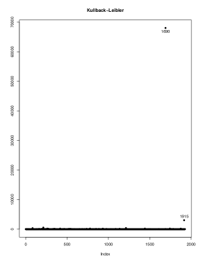
Figure 2: Kullback-Leibler divergence for the GJR-GARCH(1,1)-GED model.

The models were also compared in terms of the following information criteria, DIC (deviance information criterion), EAIC (expected AIC), EBIC (expected BIC), DIC (deviance information criterion), WAIC (Watanabe AIC) and LOOIC (leave-one-out information criterion). The results appear in Table 6. From this table we notice that the GJR-GARCH model with GED errors is clearly preferred in terms of all the criteria considered. We then proceed with the influence analysis for this model using the Kullback-Leibler divergence as described in Section 2.4 to detect influential observations. The results are depicted in Figure 2. We note that the point number 1690 (24 June 2016) is the most influential one and it represents a sharp decrease of 3.65% in the index. This is the date when the United Kingdom decided to leave the European Union.

Figure 2 about here

5 Conclusion

In this paper we discuss and compare the Bayesian estimation of GARCH models with asymmetric effects and heavy tailed distributions under different implementations of sampling the model parameters. Especifically, we implemented Zero-variance (ZV) and Hamiltonian Monte Carlo schemes for parameter estimation. Overall, the zero-variance method resulted in estimates with lower standard errors then HMC. We also proposed tools to detect influential observations.

These methods were assessed in both simulated data and real time series of returns. The simulation studies provided empirical evidence on the computational efficiency and variance reduction. The additional computational cost involved is negligible compared to that required to fit the model in the first place.

		HMC		ZV-HMC-L		ZV-HMC-Q		RWM		ZV-RWM-L		ZV-RWM-Q
N	Par	Bias	SE	Vis	SE	Vis	SE	Vis	SE	Vis	SE	Vis	SE
200	$\omega$	0.04480	0.00170	0.04480	0.00147	0.04475	0.00078	0.04479	0.00072	0.03396	0.00053	0.03684	0.00043
	$\alpha$	0.04973	0.00459	0.05019	0.00299	0.05041	0.00132	0.04972	0.00173	0.04331	0.00170	0.06101	0.00152
	$\phi$	0.10084	0.00754	0.10072	0.00465	0.10019	0.00200	0.10084	0.00274	0.10723	0.00247	0.09675	0.00219
	$\beta$	-0.32998	0.01156	-0.33024	0.00963	-0.33014	0.00479	-0.32996	0.00347	-0.27652	0.00315	-0.29693	0.00239
	$\mu$	-0.00459	0.00084	-0.00463	0.00024	-0.00463	0.00013	-0.00459	0.00182	-0.00565	0.00052	-0.00832	0.00055
500	$\omega$	0.01149	0.00071	0.01148	0.00051	0.01149	0.00026	0.01149	0.00020	0.00886	0.00017	0.01108	0.00009
	$\alpha$	0.01750	0.00347	0.01747	0.00235	0.01740	0.00074	0.01749	0.00100	0.01103	0.00077	0.01358	0.00053
	$\phi$	0.03600	0.00529	0.03612	0.00354	0.03607	0.00112	0.03600	0.00120	0.04505	0.00118	0.04486	0.00070
	$\beta$	-0.09709	0.00633	-0.09695	0.00398	-0.09698	0.00192	-0.09707	0.00190	-0.08131	0.00126	-0.09674	0.00054
	$\mu$	-0.00082	0.00054	-0.00077	0.00018	-0.00077	0.00007	-0.00081	0.00119	-0.00175	0.00019	0.00202	0.00017
1000	$\omega$	0.00191	0.00015	0.00192	0.00003	0.00192	0.00001	0.00191	0.00006	0.00175	0.00004	0.00206	0.00001
	$\alpha$	0.00712	0.00167	0.00717	0.00087	0.00707	0.00019	0.00712	0.00045	0.00346	0.00024	0.00449	0.00006
	$\phi$	0.00457	0.00274	0.00457	0.00147	0.00474	0.00038	0.00459	0.00050	0.01044	0.00038	0.00937	0.00009
	$\beta$	-0.01863	0.00172	-0.01873	0.00032	-0.01871	0.00008	-0.01863	0.00084	-0.01761	0.00031	-0.01958	0.00004
	$\mu$	-0.00082	0.00022	-0.00081	0.00008	-0.00082	0.00003	-0.00083	0.00060	-0.00130	0.00005	-0.00003	0.00002
2000	$\omega$	0.00191	0.00015	0.00192	0.00003	0.00192	0.00001	0.00191	0.00006	0.00175	0.00004	0.00206	¡0.00001
	$\alpha$	0.00712	0.00167	0.00717	0.00087	0.00707	0.00019	0.00712	0.00045	0.00346	0.00024	0.00449	0.00006
	$\phi$	0.00457	0.00274	0.00457	0.00147	0.00474	0.00038	0.00459	0.00050	0.01044	0.00038	0.00937	0.00009
	$\beta$	-0.01863	0.00172	-0.01873	0.00032	-0.01871	0.00008	-0.01863	0.00084	-0.01761	0.00031	-0.01958	0.00004
	$\mu$	-0.00082	0.00022	-0.00081	0.00008	-0.00082	0.00003	-0.00083	0.00060	-0.00130	0.00005	-0.00003	0.00002

Table 1: Results from simulations for the GJR-GARCH(1,1)-NORMAL model.

		HMC		ZV-HMC-L		ZV-HMC-Q		RWM		ZV-RWM-L		ZV-RWM-Q
N	Par	Bias	SE	Bias	SE	Bias	SE	Bias	SE	Bias	SE	Bias	SE
200	$\omega$	0.05075	0.00319	0.05271	0.00283	0.05523	0.00224	0.05065	0.00069	0.03266	0.00054	0.03650	0.00048
	$\alpha$	0.06404	0.00728	0.06571	0.00499	0.06780	0.00250	0.06399	0.00182	0.04719	0.00206	0.05936	0.00217
	$\phi$	0.13669	0.01246	0.13821	0.00804	0.13943	0.00408	0.13663	0.00283	0.13325	0.00401	0.14682	0.00419
	$\beta$	-0.35080	0.01447	-0.35216	0.01163	-0.35331	0.00578	-0.35016	0.00325	-0.28458	0.00344	-0.29983	0.00238
	$\mu$	-0.00548	0.00079	-0.00540	0.00025	-0.00534	0.00014	-0.00552	0.00163	-0.00742	0.00058	0.00058	0.00075
	$\nu$	1.65575	0.18313	1.16832	0.07342	1.07581	0.04158	1.65374	0.11214	1.28561	0.07894	1.32999	0.04894
500	$\omega$	0.01524	0.00095	0.01542	0.00073	0.01553	0.00041	0.01523	0.00020	0.01100	0.00019	0.01219	0.00010
	$\alpha$	0.02405	0.00446	0.02455	0.00299	0.02487	0.00109	0.02403	0.00100	0.01584	0.00083	0.01767	0.00068
	$\phi$	0.04640	0.00690	0.04706	0.00461	0.04720	0.00158	0.04648	0.00142	0.05328	0.00129	0.06179	0.00094
	$\beta$	-0.13184	0.00855	-0.13248	0.00603	-0.13315	0.00320	-0.13181	0.00198	-0.10612	0.00145	-0.11453	0.00068
	$\mu$	-0.00146	0.00058	-0.00146	0.00014	-0.00146	0.00006	-0.00147	0.00100	-0.00221	0.00018	0.00351	0.00019
	$\nu$	1.80807	0.14842	1.52539	0.04580	1.51592	0.01736	1.80790	0.07274	1.12321	0.04223	1.69395	0.01867
1000	$\omega$	0.00760	0.00062	0.00770	0.00038	0.00778	0.00020	0.00760	0.00013	0.00645	0.00011	0.00811	0.00003
	$\alpha$	0.01633	0.00264	0.01671	0.00180	0.01679	0.00058	0.01627	0.00044	0.01473	0.00037	0.01745	0.00020
	$\phi$	0.01324	0.00376	0.01380	0.00255	0.01385	0.00085	0.01334	0.00078	0.01686	0.00061	0.01118	0.00028
	$\beta$	-0.06116	0.00509	-0.06170	0.00283	-0.06222	0.00142	-0.06108	0.00119	-0.05559	0.00073	-0.06375	0.00019
	$\mu$	-0.00028	0.00041	-0.00031	0.00008	-0.00031	0.00004	-0.00030	0.00081	-0.00047	0.00011	-0.00198	0.00006
	$\nu$	1.27627	0.10997	1.10137	0.03210	1.09932	0.00850	1.27453	0.05149	0.60261	0.02846	1.28191	0.00547
2000	$\omega$	0.00277	0.00018	0.00275	0.00006	0.00276	0.00002	0.00277	0.00007	0.00247	0.00005	0.00319	0.00001
	$\alpha$	0.00552	0.00135	0.00541	0.00083	0.00549	0.00018	0.00553	0.00028	0.00536	0.00021	0.00573	0.00008
	$\phi$	0.01045	0.00192	0.01028	0.00114	0.01016	0.00026	0.01043	0.00054	0.01017	0.00033	0.01175	0.00012
	$\beta$	-0.02320	0.00175	-0.02296	0.00052	-0.02300	0.00016	-0.02320	0.00078	-0.02265	0.00034	-0.02671	0.00006
	$\mu$	0.00009	0.00025	0.00009	0.00004	0.00009	0.00001	0.00010	0.00060	0.00005	0.00005	-0.00001	0.00002
	$\nu$	0.62568	0.05306	0.63454	0.01529	0.63499	0.00346	0.62569	0.03418	0.37650	0.01391	0.65125	0.00174

Table 2: Results from simulations for the GJR-GARCH(1,1)-T model.

		HMC		ZV-HMC-L		ZV-HMC-Q		RWM		ZV-RWM-L		ZV-RWM-Q
N	Par	Bias	SE	Bias	SE	Bias	SE	Bias	SE	Bias	SE	Bias	SE
200	$\omega$	0.04351	0.00218	0.04319	0.00185	0.04293	0.00092	0.04351	0.00131	0.04280	0.00109	0.04838	0.00086
	$\alpha$	0.05606	0.00638	0.05583	0.00404	0.05592	0.00177	0.05619	0.00291	0.06365	0.00357	0.10990	0.00262
	$\phi$	0.12018	0.01058	0.12024	0.00655	0.12059	0.00282	0.12028	0.00453	0.19138	0.00608	0.26531	0.00529
	$\beta$	-0.32138	0.01459	-0.32042	0.01172	-0.31849	0.00549	-0.32151	0.00447	-0.32651	0.00439	-0.35433	0.00355
	$\mu$	-0.00536	0.00080	-0.00562	0.00027	-0.00555	0.00015	-0.00537	0.00164	-0.00926	0.00101	-0.00961	0.00241
	$\nu$	0.03255	0.00342	0.03285	0.00230	0.03280	0.00104	0.03268	0.02298	0.04755	0.00951	-0.02442	0.00745
500	$\omega$	0.01319	0.00074	0.01320	0.00053	0.01305	0.00029	0.01326	0.00045	0.02150	0.00039	0.02293	0.00022
	$\alpha$	0.02575	0.00375	0.02487	0.00256	0.02710	0.00084	0.02670	0.00175	0.05007	0.00152	0.08252	0.00100
	$\phi$	0.04456	0.00611	0.04423	0.00411	0.04458	0.00129	0.04439	0.00238	0.08529	0.00315	0.13963	0.00185
	$\beta$	-0.11438	0.00666	-0.11400	0.00423	-0.11380	0.00217	-0.11519	0.00284	-0.18299	0.00220	-0.20120	0.00095
	$\mu$	-0.00096	0.00059	-0.00093	0.00016	-0.00084	0.00006	-0.00095	0.00096	-0.00005	0.00034	-0.02020	0.00058
	$\nu$	0.01762	0.00283	0.01768	0.00073	0.01757	0.00031	0.01742	0.01429	-0.02632	0.00322	-0.07287	0.00154
1000	$\omega$	0.00508	0.00060	0.00515	0.00038	0.00509	0.00021	0.00508	0.00034	0.01486	0.00020	0.01842	0.00007
	$\alpha$	0.01343	0.00247	0.01328	0.00176	0.01322	0.00048	0.01343	0.00087	0.03267	0.00059	0.04156	0.00019
	$\phi$	0.01498	0.00362	0.01552	0.00244	0.01419	0.00079	0.01498	0.00156	0.03621	0.00087	0.05068	0.00037
	$\beta$	-0.04750	0.00482	-0.04640	0.00277	-0.04648	0.00144	-0.04750	0.00177	-0.11817	0.00119	-0.14952	0.00037
	$\mu$	0.00074	0.00039	0.00068	0.00010	0.00070	0.00004	0.00074	0.00077	0.00075	0.00013	-0.01364	0.00020
	$\nu$	0.00593	0.00078	0.00557	0.00033	0.00554	0.00012	0.00593	0.01004	-0.02630	0.00145	-0.02943	0.00041
2000	$\omega$	0.00241	0.00019	0.00237	0.00006	0.00239	0.00007	0.00241	0.00016	0.00449	0.00009	0.00597	0.00002
	$\alpha$	0.00694	0.00164	0.00682	0.00110	0.00614	0.00053	0.00697	0.00054	0.01664	0.00032	0.02207	0.00008
	$\phi$	0.00729	0.00171	0.00647	0.00102	0.00626	0.00034	0.00729	0.00109	0.01575	0.00049	0.02400	0.00013
	$\beta$	-0.02141	0.00174	-0.02144	0.00050	-0.02164	0.00053	-0.02150	0.00111	-0.04658	0.00054	-0.05325	0.00010
	$\mu$	-0.00073	0.00022	-0.00063	0.00004	-0.00066	0.00002	-0.00073	0.00054	-0.00044	0.00006	-0.00992	0.00007
	$\nu$	0.00360	0.00186	0.00273	0.00016	0.00271	0.00011	0.00360	0.00686	-0.02111	0.00070	-0.01191	0.00013

Table 3: Results from simulations for the GJR-GARCH(1,1)-GED model.

		HMC		ZV-HMC-L		ZV-HMC-Q		RWM		ZV-RWM-L		ZV-RWM-Q
N	Par	Bias	SE	Bias	SE	Bias	SE	Bias	SE	Bias	SE	Bias	SE
200	$\omega$	0.07396	0.00695	0.07622	0.00695	0.09096	0.00765	0.07397	0.00119	0.05184	0.00123	0.07539	0.00165
	$\alpha$	0.07271	0.00983	0.07288	0.00748	0.07262	0.00586	0.07263	0.00241	0.05137	0.00365	0.06210	0.00395
	$\phi$	0.14984	0.01694	0.14864	0.01264	0.14859	0.00934	0.15023	0.00399	0.13891	0.00512	0.14811	0.00538
	$\beta$	-0.33664	0.01721	-0.33653	0.01433	-0.33882	0.00903	-0.33654	0.00413	-0.21153	0.00457	-0.19179	0.00456
	$\mu$	-0.00305	0.00103	-0.00302	0.00053	-0.00299	0.00039	-0.00306	0.00147	-0.00492	0.00098	-0.00305	0.00125
	$\nu$	-0.37755	0.25731	-0.12751	0.20128	0.16583	0.15173	-0.38517	0.06114	-1.44091	0.05476	-2.26104	0.05945
	$\eta$	1.07731	0.20018	0.99143	0.18878	0.84586	0.13160	1.07707	0.02539	1.39641	0.02394	1.97826	0.03804
500	$\omega$	0.01564	0.00117	0.01543	0.00091	0.01534	0.00058	0.01566	0.00028	0.00901	0.00027	0.00704	0.00019
	$\alpha$	0.02713	0.00465	0.02648	0.00316	0.02601	0.00126	0.02710	0.00135	0.01687	0.00125	0.03427	0.00107
	$\phi$	0.05104	0.00740	0.05051	0.00505	0.05073	0.00201	0.05106	0.00198	0.05924	0.00177	0.05829	0.00143
	$\beta$	-0.12636	0.00895	-0.12557	0.00603	-0.12572	0.00305	-0.12648	0.00242	-0.08391	0.00193	-0.07867	0.00117
	$\mu$	-0.00201	0.00058	-0.00196	0.00019	-0.00199	0.00008	-0.00203	0.00090	-0.00273	0.00026	-0.00397	0.00024
	$\nu$	-0.49023	0.19777	-0.28602	0.11533	-0.13005	0.04942	-0.48954	0.04001	-1.40750	0.03362	-1.13249	0.02161
	$\eta$	0.29408	0.03933	0.27286	0.02951	0.24491	0.01725	0.29363	0.00417	0.30186	0.00437	0.24474	0.00351
1000	$\omega$	0.00486	0.00032	0.00479	0.00014	0.00480	0.00007	0.00485	0.00013	0.00361	0.00010	0.00218	0.00006
	$\alpha$	0.01208	0.00262	0.01187	0.00173	0.01192	0.00050	0.01206	0.00082	0.00800	0.00063	0.01531	0.00041
	$\phi$	0.02265	0.00450	0.02233	0.00289	0.02213	0.00085	0.02273	0.00103	0.02729	0.00093	0.03658	0.00058
	$\beta$	-0.04598	0.00338	-0.04576	0.00127	-0.04599	0.00054	-0.04596	0.00154	-0.03809	0.00083	-0.03356	0.00034
	$\mu$	-0.00017	0.00040	-0.00013	0.00011	-0.00012	0.00004	-0.00017	0.00064	-0.00092	0.00012	-0.00055	0.00009
	$\nu$	-0.59149	0.13937	-0.48429	0.07439	-0.41785	0.02636	-0.59531	0.02821	-1.12365	0.01765	-0.81978	0.00959
	$\eta$	0.15264	0.01502	0.14557	0.00853	0.13993	0.00266	0.15292	0.00171	0.17968	0.00170	0.12871	0.00097
2000	$\omega$	0.00201	0.00016	0.00198	0.00004	0.00198	0.00001	0.00201	0.00008	0.00163	0.00006	0.00140	0.00002
	$\alpha$	0.00690	0.00176	0.00680	0.00096	0.00685	0.00024	0.00689	0.00061	0.00189	0.00035	0.00796	0.00016
	$\phi$	0.00610	0.00310	0.00582	0.00168	0.00567	0.00048	0.00610	0.00070	0.01286	0.00052	0.01403	0.00022
	$\beta$	-0.01909	0.00188	-0.01897	0.00037	-0.01900	0.00011	-0.01908	0.00109	-0.01614	0.00047	-0.01740	0.00011
	$\mu$	-0.00038	0.00033	-0.00037	0.00007	-0.00036	0.00002	-0.00038	0.00046	-0.00084	0.00006	-0.00055	0.00003
	$\nu$	-0.62460	0.10178	-0.57874	0.05532	-0.56899	0.01670	-0.62555	0.02136	-0.99361	0.01078	-0.73694	0.00355
	$\eta$	0.10003	0.01100	0.09713	0.00644	0.09576	0.00161	0.10006	0.00083	0.12222	0.00074	0.08149	0.00026

Table 4: Results from simulations for the GJR-GARCH(1,1)-GT model.

Table 5: Parameter estimates (posterior means) and standard errors for the GJR-GARCH with normal, $t$ and GED errors.

		HMC	SE	ZV-HMC-L	SE	ZV-HMC-Q	SE
	$\omega$	0.04289	0.00005	0.04282	0.00001	0.042807	$<$0.00001
	$\alpha$	0.00623	0.00023	0.00558	0.00007	0.005423	0.00002
Normal	$\phi$	0.26407	0.00018	0.26416	0.00007	0.264357	0.00002
	$\beta$	0.81459	0.00018	0.81491	0.00003	0.815006	0.00001
	$\mu$	0.03091	0.00036	0.03114	0.00001	0.031127	$<$0.00001
	$\omega$	0.03772	0.00008	0.03791	0.00001	0.03799	0.00001
	$\alpha$	0.00728	0.00014	0.00682	0.00008	0.00635	0.00007
$t$	$\phi$	0.32830	0.00071	0.32965	0.00045	0.33049	0.00004
	$\beta$	0.79973	0.00038	0.79928	0.00005	0.79925	0.00002
	$\mu$	0.05480	0.00025	0.05441	0.00006	0.05429	0.00000
	$\nu$	5.84457	0.00505	5.83454	0.00518	5.84157	0.00133
	$\omega$	0.04085	0.00013	0.04079	0.00002	0.04081	0.00002
	$\alpha$	0.00719	0.00011	0.00705	0.00006	0.00682	0.00004
GED	$\phi$	0.30951	0.00053	0.30834	0.00022	0.30894	0.00019
	$\beta$	0.79975	0.00045	0.80000	0.00005	0.79997	0.00002
	$\mu$	0.04607	0.00019	0.04675	0.00005	0.04664	0.00002
	$\nu$	0.64646	0.00021	0.64610	0.00006	0.64622	0.00005
	$\omega$	0.03833	0.00006	0.03787	0.00003	0.03788	0.00002
	$\alpha$	0.00665	0.00023	0.00620	0.00010	0.00648	0.00009
GT	$\phi$	0.33283	0.00025	0.33236	0.00024	0.33171	0.00014
	$\beta$	0.79881	0.00027	0.79945	0.00007	0.79943	0.00002
	$\mu$	0.05460	0.00028	0.05470	0.00005	0.05482	0.00002
	$\nu$	2.63386	0.01477	2.65813	0.00773	2.64935	0.00243
	$\eta$	1.04019	0.00209	1.03909	0.00084	1.03949	0.00029

Table 6: EAIC, EBIC, DIC, WAIC and LOOIC values for the estimated GJR-GARCH(1,1) models.

	DIC	EAIC	EBIC	WAIC	LOOIC
GJR-GARCH(1,1)-NORMAL	4687.4	4691.5	4713.8	4689.9	4689.9
GJR-GARCH(1,1)-T	4594.8	4600.1	4627.9	4595.4	4595.4
GJR-GARCH(1,1)-GED	4592.4	4597.5	4625.3	4593.1	4593.1
GJR-GARCH(1,1)-GT	4596.2	4603.6	4637.0	4596.9	4590.9

Figure 1: S&P500 time series returns from Oct 6, 2009 to June 2, 2017.

References

- Assaraf and Caffarel (1999) R. Assaraf and M. Caffarel. Zero-Variance principle for Monte Carlo algorithms. Physical Review Letters, 83(23):4682–4685, 1999.
- Assaraf and Caffarel (2003) R. Assaraf and M. Caffarel. Zero-variance zero-bias principle for observables in quantum Monte Carlo: application to forces. The Journal of Chemical Physics, 119(20):10,536–10,552, 2003.
- Bollerslev (1986) T. Bollerslev. Generalized autoregressive conditional heteroskedasticity. Journal of Econometrics, 31:307–327, 1986.
- Engle (1982) R. F. Engle. Autoregressive conditional heteroscedasticity with estimates of the variance of United Kingdom inflation. Econometrica, 50:987–1007, 1982.
- Girolami and Calderhead (2011) M. Girolami and B. Calderhead. Riemann manifold Langevin and Hamiltonian Monte Carlo methods. Journal of the Royal Statistical Society B, 73:123–214, 2011.
- Glosten et al. (1993) L. R. Glosten, R. Jagannathan, and D. E. Runkle. On the relation between the expected value and the volatility of the nominal excess returns on stocks. The Journal of Finance, 48:1791–1801, 1993.
- Hao et al. (2016) Hong-Xia Hao, Jin-Guan Lin, Hong-Xia Wang, and Xing-Fang Huang. Bayesian case influence analysis for GARCH models based on Kullback-Leibler divergence. Journal of the Korean Statistical Society, 45(4):595–609, 2016.
- Leimkuhler and Reich (2004) Benedict Leimkuhler and Sebastian Reich. Simulating Hamiltonian dynamics, volume 14 of Cambridge monographs on applied and computational mathematics. Cambridge University Press, Cambridge, 2:18, 2004.
- McDonald and Newey (1988) J. B. McDonald and W. K. Newey. Partially adaptive estimation of regression models via the generalized distribution. Econometric Theory, 4:428–457, 1988.
- Mira et al. (2013) A. Mira, R. Solgi, and D. Imparat. Zero variance Markov chain Monte Carlo for Bayesian estimators. Statistics and Computing, 23(5):653–662, 2013.
- Neal (2011) R. M. Neal. MCMC using Hamiltonian dynamics. In Handbook of Markov chain Monte Carlo, pages 113–162. Boca Raton: Chapman and Hall-CRC Press, 2011.
- Oates et al. (2016) C. J. Oates, M. Girolami, and N. Chopin. Control functionals for Monte Carlo integration. Journal of the Royal Statistical Society: Series B (Statistical Methodology), 79(3):695–718, 2016.
- Papamarkou et al. (2014) T. Papamarkou, A. Mira, and M. Girolami. Zero variance differential geometric Markov chain Monte Carlo algorithms. Bayesian Analysis, 9(1):97–128, 2014.
- R Development Core Team (2015) R Development Core Team. R: A language and environment for statistical computing. R Foundation for Statistical Computing, Vienna, Austria, 2015.
- Santos and Bolfarine (2016) B. Santos and H. Bolfarine. On Bayesian quantile regression and outliers. ArXiv e-prints, jan 2016.
- Teräsvirta (2009) T. Teräsvirta. An introduction to univariate garch models. In Davis R.A. Kreiss J.-P. Mikosch T. (Eds.) Andersen, T.G., editor, Handbook of Financial Time Series, pages 17–42. Springer, 2009.
- Tsay (2010) R. S. Tsay. Analysis of Financial Time Series. John Wiley & Sons, third edition, 2010.
- Virbickaitė et al. (2015) A. Virbickaitė, M. C. Ausin, and P. Galeano. Bayesian inference methods for univariate and multivariate GARCH models: a survey. Journal of Economic Surveys, 29(1):76–96, 2015.