Nonparametrically estimating dynamic bivariate correlation using visibility graph algorithm

Abstract

Dynamic conditional correlation (DCC) is a method that estimates the correlation between two time series across time. Although used primarily in finance so far, DCC has been proposed recently as a model-based estimation method for quantifying functional connectivity during fMRI experiments. DCC could also be used to estimate the dynamic correlation between other types of time series such as local field potentials (LFP’s) or spike trains recorded from distinct brain areas. DCC has very nice properties compared to other existing methods, but its applications for neuroscience are currently limited because of non-optimal performance in the presence of outliers. To address this issue, we developed a robust nonparametric version of DCC, based on an adaptation of the weighted visibility graph algorithm which converts a time series into a weighted graph. The modified DCC demonstrated better performance in the analysis of empirical data sets: one fMRI data set collected from a human subject performing a Stroop task; and one LFP data set recorded from an awake rat in resting state. Nonparametric DCC has the potential of enlarging the spectrum of analytical tools designed to assess the dynamic coupling and uncoupling of activity among brain areas.

Introduction

Estimation methods for dynamic bivariate correlation in resting state fMRI have been gaining increasing attention in the neuroimaging community. Dynamic correlation estimation is of interest because many recent studies have identified dynamic changes in functional connectivity during the course of an fMRI experiment [1-7], especially during resting state. Estimating dynamic correlation is of interest in neuroscience in general. For example, dynamic correlation between local field potential time series obtained from different brain regions could be used to explore how certain brain regions work in tandem during certain specific behaviors. When identifying such changes, it is of importance to ensure that the dynamic shifts in the correlations observed are not due to spurious fluctuations inherent to the estimation method used. This fact underlines the need for assessing the accuracy of existing estimation methods and for developing accurate new methods.

Recently Lindquist and co-authors [8] published an expository paper in which they recommended using the dynamic conditional correlation (DCC) method [9,10] as the best approach for estimating the temporal evolution of the correlation between two time series. Two other methods that Lindquist and co-authors considered were the commonly used sliding window technique and the exponential weighted moving average (EWMA) technique. Using a simulation study and real-data examples, Lindquist et al. [8] illustrated that DCC performed far better when compared to the other two methods.

DCC is widely used in scientific fields other than neuroscience (e.g. finance), but it has some often overlooked shortcomings. DCC is a parametric method, in which the parameters involved are estimated using a 2-stage maximum likelihood (ML) method. The optimization task in the ML method is conducted using numerical iteration methods for which initial values for the parameters have to be provided. Numerical convergence of these methods typically does not depend on the starting points. However, while working on the real-data examples and simulations for this paper, we encountered a few scenarios where convergence (or rather non-convergence) could pose a problem, at least for the iterative methods used in two different R packages available for DCC: ccgarch and rmgarch.

A distinct and more important issue with the parameter framework of DCC is its sensitivity to extreme values, which do occur in time series measurements and can be ignored only if such values are an anomaly that does not make sense with the underlying scientific framework. A good example comes from financial time series. Any financial time series based on US markets (e.g. S$\&$P index) had a few extreme values during the 2008 market crash. Dynamic correlations considered for such a pair of time series, if including the values from 2008, cannot ignore those extreme values, because they are real. Time series examples with normally occurring extreme values in neuroimaging and neuroscience are not uncommon either, as seen, for example, in the LFP time series data, which is one of the data sets analyzed in this paper.

To address these problems, we propose a novel nonparametric approach for estimating dynamic correlation estimation which we refer to as nonparametric weighted visibility graph algorithm (nonparametric WVGA). Our method is based on an adaptation of the visibility graph algorithm (VGA), introduced by physicists, Lacasa and co-authors [11]. VGA’s general approach is to convert time series into mathematical graphs, a procedure that does not involve any parameters. Therefore, our new method is nonparametric in nature and robust to extreme values. We illustrate the utility of this method via simulations and real data examples.

Methods

For the current work, we considered three methods for estimating dynamic correlation (Figure 1). The first two methods - the SW and DCC - are currently existing methods and here we followed closely the exposition and notation used in Lindquist et al [8]. The third method based on weighted visibility graph algorithm is our new approach to the dynamic-correlation-estimation problem.

We illustrate the methods using two time series generated as in Lindquist et al’s [8] simulations study $\#1$. Random data were generated for each time point using a mean-zero bivariate normal distribution, with correlation matrix set to

$$\left[\begin{array}[]{cc}\sqrt{2}&0\\ 0&\sqrt{3}\end{array}\right].$$

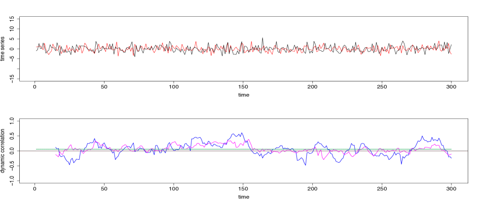
A bivariate time series generated using the above mechanism with $T=300$ time points is shown in the top panel in Figure 1. The dynamic correlation was a priori set to zero in this simulated example. That is, the underlying correlation of this simulated bivariate time series equals zero at all points in time.

Figure 1: Top panel: The two time series used for the first illustrative simulated example; data were generated from a bivariate normal distribution. Bottom Panel: Dynamic correlations estimated for the above two time series using 3 different methods: method $\#$1, SW (blue); method $\#$2, DCC (green); and method $\#$3, nonparametric WVGA (magenta). The black horizontal line in the center through zero represents the underlying true dynamic correlation for this example.

Method $\#$ 1 - Sliding-Window (SW) technique

SW technique [1,2,4] is easy to explain and implement. We chose a window-frame of size “$ws$” = 15 for the example considered in figure 1. At the first iteration, we used the window-frame to frame the first ($ws=$) 15 time points of the bivariate time series, and find the correlation between the values of the two series within this window-frame. Then we repeat the process by sliding the window to the right, one unit at a time. Thus, in general, at iteration $i$, the right-end of the SW was placed at the $(i-1+ws)^{th}$ time point of both time series, and the correlation between the two time series within the window-frame was calculated. This series of correlations forms the blue curve plotted in the bottom-panel of Figure 1.

To make it clearer, the $1^{st}$ correlation value is the correlation between two vectors each of length 15, each containing the values corresponding to time points between 1 and 15 (end points included) of the $1^{st}$ and the $2^{nd}$ time series, respectively. To obtain the second correlation, we moved the window one unit to the right, so that for this second iteration the right-end of the window-frame is at time-point 16, and the left end is at time-point 2. The $2^{nd}$ correlation value will be the correlation between two vectors each of length 15, each containing the values corresponding to time points between 2 and 16 (end points included) of the $1^{st}$ and the $2^{nd}$ time series, respectively. We continued moving the SW one unit to the right at each iteration and calculated the corresponding correlation until the final iteration (that is, when the right-end of the SW is at $T=300^{th}$ time point). The performance of this method depends on the size of the window: a larger $ws$ provides smoother estimates of dynamic correlation, while smaller $ws$ is more sensitive to variations in the underlying data. Lindquist et al [8] discusses this issue in more detail, and also mentions variations of the above technique such as tapered sliding window [1].

Method $\#$ 2 - Dynamic conditional correlation

DCC is a multivariate volatility model commonly used in financial analyses, which also has neuroimaging applications. Lindquist et al provides an accessible exposition of DCC using mathematical notation. The original papers by Engle and Sheppard [9, 10] are also good sources on DCC. As mentioned in Lindquist et al, “DCC provides a parametric approach towards estimating dynamic correlations, much like auto-regressive (AR) and auto-regressive moving average (ARMA) models provide a parametric approach towards modeling fMRI noise [12]”. In particular, DCC is based on generalized autoregressive conditional heteroscedastic (GARCH) models [13], which were developed to incorporate the so-called “stylized facts” (i.e. statistical irregularities) common to a large number of financial time series [14]. The key feature of DCC that we would like to emphasize here is that it is parametric. The parameters in DCC are estimated using a two step ML estimation approach, the mathematical details of which can be found in Lindquist et al. We will not repeat this description but instead we will explain how DCC estimation can be performed using the R packages ccgarch and rmgarch.

Two R packages - ccgarch and rmgarch - have been developed for applying the DCC method. The main function for DCC estimation in ccgarch is called ‘dcc.estimation’. The inputs required for this R function are the initial values for the GARCH parameters (see equations 19 and 20 in Lindquist et al) [8]; the specification of the numerical optimization routine for maximizing the log-likelihood; and the two time series whose dynamic correlation is to be estimated. In our own analyses, we used the Broyden-Fletcher-Goldfarb-Shannon (BFGS) algorithm and the diagonal model for GARCH covariance matrix mentioned in Lindquist et al., specified using model = “diagonal” argument within the dcc.estimation function. Among the many outputs provided by dcc.estimation, the most relevant for the current work is the one named DCC which stores the dynamic conditional correlation as a time series vector in R.

The main function for DCC estimation in rmgarch is called ‘dccfit’. This function requires three inputs: specification of the model, the multivariate time series, and a solver to be used for optimization. In our work, we specified the model by using a separate command called ‘dccspec’; the GARCH part of the specification was accomplished by using ugarchspec. The optimization method employed in all our simulations and examples was the default named ‘solnp’ which performs nonlinear optimization using augmented Lagrange multiplier method [15].

A key point is that in the original DCC model presented by Engle and Sheppard [9, 10] multivariate normality of the underlying pair of time series was assumed for ML estimation. As mentioned in the same papers [9, 10], multivariate normality is not necessary for statistical consistency of the estimators, as the estimation can be extended to a quasi-likelihood framework. However, even in the quasi-likelihood framework, certain assumptions (e.g. related to the moments) are often necessary. Such assumptions may not be valid for time series which contain extreme values.

Method $\#$ 3 - Nonparametric weighted VGA (WVGA)

As mentioned above, DCC depends on assumptions of normality or at least finiteness of moments. To avoid dependence of such assumptions, in our new method both time series were converted into graphs using the weighted visibility graph algorithm (WVGA), introduced in Supriya et al [16]. WVGA, developed by Lacasa et al [11], is an extension of the visibility graph algorithm that converts simply but elegantly a time series to a graph. Methods based on visibility graphs have become popular after the original concept of mapping time series to a complex network was introduced in Zhang and Small [17]. The nodes of the WVGA-based graphs correspond to the time points and therefore, the graph generated from each time series consists of $T$ nodes. The weight $w_{ab}$ of the edge between the nodes corresponding to time points $t_{a}$ and $t_{b}$, with $a<b$, is calculated using equation (2) given in p.6558 in Supriya et al [16]:

$$w_{ab}=\arctan{\frac{x(t_{b})-x(t_{a})}{t_{b}-t_{a}}}.$$

Here $x(t_{a})$ and $x(t_{b})$ are the values of the time series at time points $t_{a}$ and $t_{b}$, respectively. All edge weights are calculated in radians.

We modified WVGA in several ways. First, strictly speaking, for the graph to be a visibility graph, there should be no edge between two nodes if there is no “visibility” between them, where “visibility” is defined based on the criterion spelled out in Lacasa et al.[11]. However, in our version of the algorithm we kept all the edges, and each edge had an assigned weight based on the arctan function mentioned above. Since this algorithm is very similar to the one proposed in Supriya et al. [16], we retain the name ”weighted visibility graph algorithm”. Second, while Supriya et al. [16] used only the absolute values of the weights, we retained the signs of the weights calculated, as is. The reason we introduced these modifications is that the shape of the arctan function, rather than the visibility criterion, provides a suitable solution for our purpose. We elaborate more on this in the discussion section.

Our modified WVGA for dynamic correlation estimation is also based on a sliding window. As for method 1, we picked a window of size 15 for illustration. Associated with each time point $t_{i}$ (that is, with each node $n_{i}$ in the WVGA graph) is a weight-vector of length $T$ consisting of the weights of the edges from all the other nodes of the graph to $n_{i}$. We named this weight vector as $\mathbf{w}_{i}$. Note that we considered the weight between $n_{i}$ to itself as zero. That is, $i^{th}$ element of $\mathbf{w}_{i}$ is zero, for all $i$. For each time series, we place the right-end of a sliding window (of size 15) at time point $i$, considered all the weight vectors

$$\left\{\mathbf{w}_{i-15+1},\mathbf{w}_{i-15+2},\ldots,\mathbf{w}_{i}\right\},$$

and obtained a new vector $\mathbf{W}_{(i\mathrel{\mathop{\mathchar 58\relax}}\,\mathrm{median})}$ by taking the median element-wise. That is $k^{th}$ element of $\mathbf{W}_{(i\mathrel{\mathop{\mathchar 58\relax}}\,\mathrm{median})}$ is the median of the $k^{th}$ elements of $\left\{\mathbf{w}_{i-15+1},\mathbf{w}_{i-15+2},\ldots,\mathbf{w}_{i}\right\}.$ If we use super-scripts to denote the vectors corresponding to the two time series, then the above steps may be summarized using the following formula:

$$\mathbf{W}^{(j)}_{(i\mathrel{\mathop{\mathchar 58\relax}}\,\mathrm{median})}[k]=\mathrm{median}{\left\{\mathbf{w}^{(j)}_{i-15+1}[k],\mathbf{w}^{(j)}_{i-15+2}[k],\ldots,\mathbf{w}^{(j)}_{i}[k]\right\},}$$

where $k(=1,\ldots,T)$ denotes the $k^{th}$ element of each vector and $j(=1,2)$ denote the $j^{th}$ time series. The correlation at the $i^{th}$ iteration (where $i$ ranges from 15 to $T$) is then just the correlation between the vectors $\mathbf{W}^{(1)}_{(i\mathrel{\mathop{\mathchar 58\relax}}\,\mathrm{median})}$ and $\mathbf{W}^{(2)}_{(i\mathrel{\mathop{\mathchar 58\relax}}\,\mathrm{median})}$.

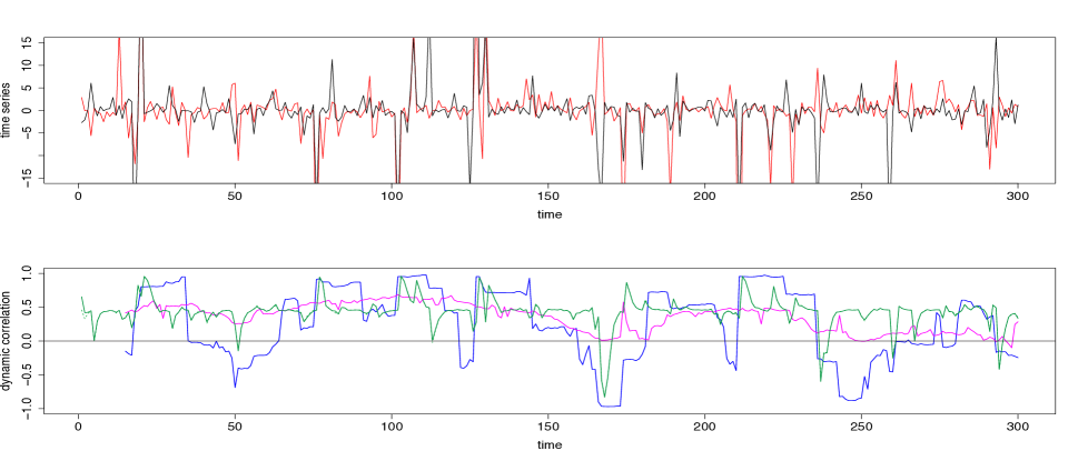
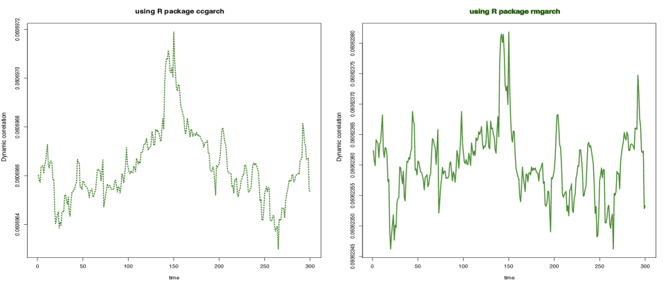
To illustrate graphically how the three methods perform, we computed the three dynamical correlations and plotted them together in the bottom panel of Figure 1. The underlying dynamic correlation, which is equal to zero at all time points, is plotted as the black line. The correlations obtained through the SW method are plotted as the blue line. There are two superimposed green lines corresponding to the two R packages used for DCC estimation - ccgarch and rmgarch. The lines superimpose because in this case the two results coincide. However, this is not always the case with real data example, as it will be seen below. The green curves may appear to be straight lines, but this is not in fact the case (see Figure A1 in the Appendix where we used a different scale for the y-axis). The correlations obtained through the nonparametric WVGA method are plotted as the magenta curve.

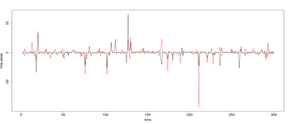
SW method (blue curve) results in the worst estimate, DCC method (green curves) results in the best estimate, and the nonparametric WVGA method (magenta curve) performs somewhere in between. This qualitative estimation is confirmed quantitatively by the following summary statistics: mean absolute value of the blue curve is 0.19, for both green curves is 0.06, and for the magenta curve is 0.10; the maximum value for the blue, (both) green, and magenta curves are, respectively, 0.61, 0.06, and 0.39. In the above example, DCC performs better than both the SW technique and our new method. However, the data in this example are a pair of nicely behaved time series with no outliers (since they were generated from a bivariate normal density). In the presence of outliers DCC does not perform as well. We generated two time series from a bivariate Cauchy density (by using the R function rcauchy2d from the package fMultivar). Because Cauchy density has very heavy tails, the generated data contain several extreme values.The correlation parameter for the bivariate Cauchy density ($\rho$) was set to zero, so that the underlying dynamic correlation for this example was also zero for all time points. The two time series thus generated are plotted in the top panel in Figure 2. We applied the same three analytical methods to this data set and the results are plotted in the bottom panel in Figure 2, with the same color coding as in Figure 1. For this example, the new method easily outperformed the other two methods. The mean absolute values for the blue, green, and magenta curves were, respectively, 0.50, 0.46 (for both green curves) and 0.35; the corresponding maximums of the absolute values of the correlations were 0.98, 0.96 (for both green curves) and 0.67, respectively. Thus, the new method, nonparametric in nature, was more robust when extreme values were present in the data. As a minor note, the y-axes for the top panels had the same scale for Figures 1 and 2, which cut off the plot for some extreme values in Figure 2. In order to see the actual extreme values, we plotted the same pair time series with extended y-margins in Appendix Figure A2 .

Figure 2: Top panel: The two time series used for the second illustrative simulated example; data were generated from a bivariate Cauchy distribution. Bottom Panel: Dynamic correlations estimated for the above two time series using various methods. Method $\#$1, SW (blue), method $\#$2, DCC (green), and method $\#$3, based on modified WVGA (magenta). The black horizontal line in the center through zero represents the underlying true dynamic correlation for this example.

Simulation design

To assess the performance of the three methods under various scenarios, we ran extensive simulations using scenarios aimed to closely match the work of Lindquist et al[8]. We therefore generated data by using bivariate normal distribution, as in Lindquist et al[8], but also bivariate Cauchy distribution, to obtain data sets with extreme values. In all the simulations involving bivariate Cauchy, values exceeding 50 were reset to 50, and values below -50 were reset to -50. The means for all pairs of time series in the simulation study was set to $(0,0)$ across all time points and the covariance matrix at time point $t$ was

$$\left[\begin{array}[]{cc}2&\sqrt{6}p(t)\\ \sqrt{6}p(t)&3\end{array}\right].$$

By considering three different forms for $p(t)$ we obtained three different simulations scenarios, as in Lindquist et al [8]. For simulations involving the sliding window technique (method1) and the nonparametric WVGA (method3), the window size was set to 15.

Simulations Design D1: In this case, we set $p(t)=0$ for all $t$ as in the illustrative examples above. We considered four time series of different lengths ($T=150,300,600$ and $1000$) for both bivariate normal and bivariate Cauchy distributions. The metrics used to assess the performance of the methods for this scenario were the mean and maximum across all time points.

Simulations Design D2: The scenarios in $D2$ were designed to assess the performance of the methods when the underlying correlation varies slowly over time. We set $p(t)=\sin\left(t/\Delta\right)$, $\Delta=1024/2^{k}$, with $k=3,4$. We obtained two different (sub-)scenarios corresponding to $k=3$ and $4$, which we refer to as $D2a$ and $D2b$. We set $T=600$ for both of these sub-scenarios. The metric used to assess the performance was mean-squared-error (MSE) as in Lindquist et al.

Simulations Design D3: The scenarios in $D3$ were designed to assess the performance of the methods when there is a rapid change in the underlying correlation; here, the rapid change occurs near time point 250. We set $p(t)$ equal to a Gaussian kernel with mean 250 and standard deviation 15$k$, where $k$ = 3 and 4. The two $k$’s resulted in two different (sub-)scenarios, $D3a$ and $D3b$; $T=600$ for both cases. MSE was used to compare the performance of the methods.

Real data analysis

To illustrate the advantages and disadvantages of the methods considered in this paper, we applied our analysis to two different empirical data sets. The first data set used for illustration was fMRI data collected from one healthy adult subject while the subject performed a color-word Stroop task [18]. The data were part of a sample collected for a study of the underlying mechanisms based on distributed network of brain regions involved in congruency sequencing effect in cue-conflict paradigms [19]. Time series from six different brain regions were used in our analysis, and dynamic correlations between each pair of regions were obtained. The second data set used for illustration consisted of local field potential (LFP) time series [20, 21] obtained from four different electrodes implanted in the brain of a rat. The recording occurred while the rat was awake and placed on a small platform in the lab. Three of the recordings were from the CA1 field of the hippocampus, and one recording from the medial dorsal striatum. Dynamic correlations of data from each pair of recordings were computed. Although the behavior of the dynamic correlations of pairwise time series was of intrinsic interest for the background scientific research question related to fMRI and LFP data sets, the main purpose in the current analysis was to illustrate various aspects associated with the estimation methods considered in this paper. Specifically, the Stroop task fMRI data set illustrated the convergence issues related to DCC and LFP data illustrated the performance of the methods in the presence of extreme values. Details about data extraction for fMRI data set and recording for the LFP data are presented below.

fMRI data. Sample fMRI data from one healthy human adult subject were downloaded from OpenfMRI.org. We used Stroop task fMRI data (https://openfmri.org/dataset/ds000164/) [19], since activation patterns for the Stroop task are relatively well known. Preliminary data processing followed previous publication [22]. Using FMRIB Software Library (FSL) as well as Analysis of Functional NeuroImages (AFNI), anatomical volume was skull stripped, segmented (gray matter, white matter and CSF), and registered to the MNI 2mm standard brain. Processing of fMRI echo planar image (EPI) volume included the following. The first four EPI volumes were removed; transient signal spikes were removed; head motion was corrected; the volumes were smoothed with a 6mm FWHM Gaussian kernel; the volumes were resampled, spatially transformed and aligned to the MNI 2mm standard brain space; volumes with excess motion were scrubbed. In order to extract the time series for six regions chosen a priori, the frontal medial cortex, subcallosal frontal region, insular cortex, Heschl’s gyrus, and amygdala were defined using the Harvard-Oxford atlas and the Caudate Head was defined using WFU PickAtlas.The EPI time series was extracted within each of these six regions.

LFP data. The local field potential (LFP) data were recorded from an awake rat placed on a small platform. Previous to the recording, the animal had been implanted with a 16 tetrode hyperdrive assembly intended for recording in the CA1 field of the hippocampus, combined with two cannula/electrode systems (PlasticsOne, Inc) aimed bilaterally at the medial dorsal striatum. The tetrodes were gradually lowered in the CA1 layer across 8 to 10 days after recovery from surgery, and their tip was positioned based on the configurations of sharp waves and ripples. The electrodes aimed at the dorsal striatum were implanted directly in the position from which the recording was obtained (AP: + 2.5mm, ML: +/-2.4mm; DV: -5.4mm; tilted 22 degrees from the vertical in the sagittal plane). The single wire electrodes located in the striatum and the 16 tetrodes were connected through a PCB to a group of four headstages with a total of 64 unity gain channels and 2 color LEDs for position tracking. The LFP signals were amplified (1000x), band-pass filtered (1-1000Hz), digitized (30KHz), and stored together with LED positions on hard disk (Cheetah Data Acquisition System, Neuralynx, Inc.). Subsequently the signal was downsampled to 1KHz, in which form it was used for the current analysis.

Results

Simulations

Simulations Design D1: Results from simulations with design D1 are presented in tables 1 and 2. Table 1 presents the results when the pair of time series was generated from a bivariate normal distribution and table 2 presents the results related to bivariate Cauchy. Note that one of the two DCC estimates consistently had convergence problems. In the bivariate normal case, across all T values, DCC performed best, SW performed worst, and nonparametric WVGA’s performance was in between. In the bivariate normal case, DCC’s performance improved with larger T as measured both by bias and variance, while that of SW and nonparametric WVGA methods remained the same for all T. In the bivariate Cauchy case, the SW method performed consistently worst across all T, while for the other two methods performance improved with larger T. At small T values, the nonparametric WVGA method performed better than the DCC method. As T became larger, the DCC performance overtook that of WVGA, and at T = 1000, DCC performed better than WVGA even if compared by using MSE: [$(0.200^{2})+(0.035^{2})]\;=\;0.041$ versus [$(0.126^{2})+(0.084^{2})]\;=\;0.023$. Thus, in the presence of extreme values, DCC was robust as long as the number of time points was large enough; when the number of time points was small, WVGA-based evaluation is preferable to DCC.

Table 1. Bivariate Normal in design D1
Mean of absolute value of correlations across time
	T = 150	T = 300	T = 600	T = 1000
SW	$0.218(0.039)$	$0.217(0.027)$	$0.218(0.019)$	$0.218(0.015)$
WVGA-based	$0.134(0.033)$	$0.129(0.021)$	$0.127(0.015)$	$0.125(0.012)$
DCC1	$0.071(0.053)$	$0.051(0.037)$	$0.037(0.025)$	$0.029(0.020)$
DCC2	$0.077(0.052)$	$0.055(0.037)$	$0.040(0.025)$	$dnc^{*}$
Maximum of absolute value of correlations across time
	T = 150	T = 300	T = 600	T = 1000
SW	$0.616(0.094)$	$0.670(0.075)$	$0.717(0.065)$	$0.744(0.053)$
WVGA-based	$0.392(0.080)$	$0.425(0.067)$	$0.455(0.058)$	$0.475(0.054)$
DCC1	$0.093(0.101)$	$0.075(0.087)$	$0.067(0.077)$	$0.055(0.068)$
DCC2	$0.139(0.140)$	$0.111(0.115)$	$0.104(0.105)$	$dnc^{*}$
$*dnc$ = did not converge

Table 2. Bivariate Cauchy in design D1
Mean of absolute value of correlations across time
	T = 150	T = 300	T = 600	T = 1000
SW	$0.531(0.080)$	$0.529(0.057)$	$0.526(0.040)$	$0.528(0.030)$
WVGA-based	$0.244(0.098)$	$0.222(0.067)$	$0.210(0.048)$	$0.200(0.035)$
DCC1	$0.292(0.188)$	$0.224(0.143)$	$0.168(0.111)$	$0.126(0.084)$
DCC2	$dnc*$	$dnc$	$dnc$	$dnc$
Maximum of absolute value of correlations across time
	T = 150	T = 300	T = 600	T = 1000
SW	$0.973(0.030)$	$0.986(0.012)$	$0.992(0.005)$	$0.994(0.003)$
WVGA-based	$0.540(0.121)$	$0.558(0.097)$	$0.576(0.081)$	$0.590(0.074)$
DCC1	$0.363(0.279)$	$0.321(0.281)$	$0.302(0.289)$	$0.245(0.267)$
DCC2	$dnc$	$dnc$	$dnc$	$dnc$
$*dnc$ = did not converge

(a)

(b)

(c)

(d)

Figure 3: Results for single iteration from simulations design D2. Top row: Underlying pair of time series from bivariate normal. Bottom row: Underlying pair of time series from bivariate Cauchy. Left column: Design 2a ($k=3$). Right column: Design 2b ($k=4$). The underlying true dynamic correlations are plotted as the black curve. Blue (SW), magenta (WVGA), green solid (DCC with rmgarch) and green dashed (DCC with ccgarch) represents the estimates of dynamic correlation.

(a)

(b)

(c)

(d)

Figure 4: Boxplots of mean squared error of the estimation methods based on 1000 iterations from simulations design D2. The panels correspond to bivariate Normal (top row), bivariate Cauchy (bottom row), design D2a (left column) and design D2b (right column), as in figure 3.

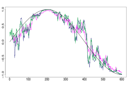
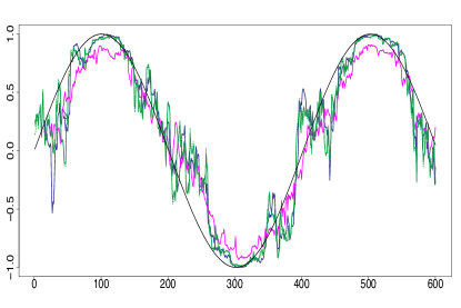
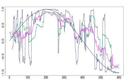
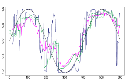
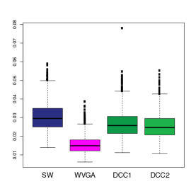
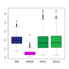
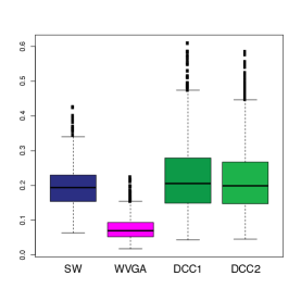
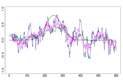
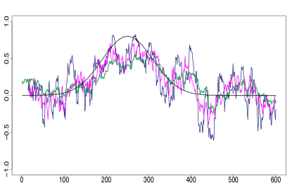
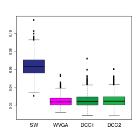
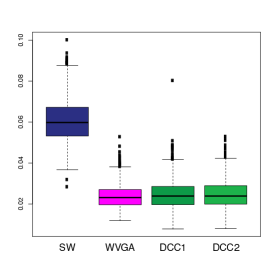
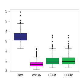
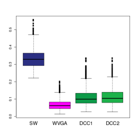
Simulations Design D2: In Figure 3, the black curves in the left panels are the underlying true dynamic correlations corresponding to simulations design D2a, the black curves in the right panels correspond to that of the simulations design D2b. Each panel refers to a single simulation iteration. The estimates of the dynamic correlations obtained via the three methods presented in this paper are plotted as colored curves. The top panels correspond to the bivariate normal scenario and the bottom panels correspond to the bivariate Cauchy scenario. Results from 1000 simulations for each scenario are plotted in Figure 4. In this design, the performance of the WVGA-based method was far superior to the other two methods for both bivariate normal and bivariate Cauchy simulations.

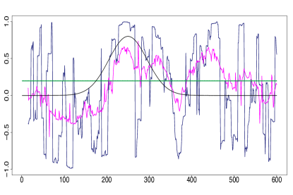
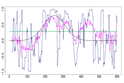
Simulations Design D3: Figure 5 plots the underlying true dynamic correlations and the estimates based on the three methods for a single iteration corresponding to the simulation design D3. Interestingly, the DCC estimates based on both R packages (the green straight lines) did not capture the dynamic shift in correlations at all. The results based on 1000 iterations are plotted in Figure 6. In all four scenarios for the design (D3a and D3b, bivariate normal and Cauchy), the performance of SW was substantially worse compared to the other two methods. DCC’s performance was comparable to that of nonparametric WVGA method in the bivariate normal scenario, although the WVGA method had a slight edge over DCC. In the bivariate Cauchy case (bottom panels) the improvement in performance for the WVGA-based method is more substantial. Thus, the results of the simulations indicate that when the underlying dynamic correlations are not constant across time, nonparametric WVGA performed better than DCC in many of the scenarios, and never worse than DCC in any of the scenarios considered.

(a)

(b)

(c)

(d)

Figure 5: Results for single iteration from simulations design D3. Top row: Underlying pair of time series from bivariate Normal. Bottom row: Underlying pair of time series from bivariate Cauchy. Left column: Design 3a (that is, $k=3$). Right column: Design 3b ($k=4$). The underlying true dynamic correlations are plotted as the black curve. Blue (SW), magenta (WVGA), green solid (DCC with rmgarch) and green dashed (DCC with rmgarch) represents the estimates of dynamic correlation.

(a)

(b)

(c)

(d)

Figure 6: Boxplots of mean squared error of the estimation methods based on 1000 iterations from simulations design D3. The panels correspond to bivariate normal (top row), bivariate Cauchy (bottom row), design D3a (left column) and design D3b (right column), as in figure 5.

Stroop task data

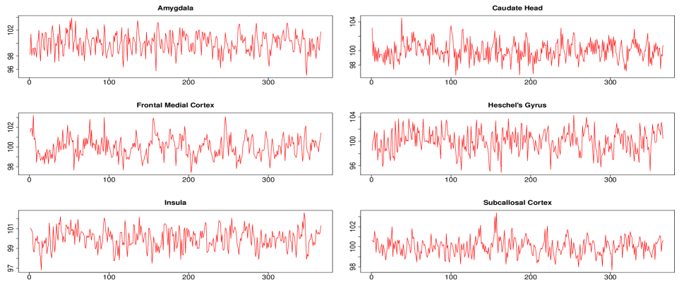
The six times series obtained from six different brain regions of a single subject are shown in Figure 7. Since these data plots did not show the presence of any extreme values, we would expect the estimates from DCC to be our most accurate estimate of the true underlying correlations. The results of this data analysis were useful in illustrating the non-convergence problem related to DCC.

Figure 7: Time series from six regions in Stroop task fMRI data

Pairwise dynamic correlation plots are shown in Figure 8. Based on the conclusions from our simulation study, the results of the DCC estimation are likely to be the best estimate of the true dynamic correlation. The results partially validate this expectation. On average, estimates based on SW, DCC obtained by using the rmgarch package in R, and WVGA (blue, solid green, and magenta curves, respectively) indicate roughly similar values, although the DCC estimate is more or less constant across time while the SW and WVGA estimates fluctuate over time. However, the DCC estimates obtained using the ccgarch R package(dotted green lines in Figure 8) were markedly different from the results of the same analysis based on the rmgarch package. For all pairwise comparisons, the cc-garch based DCC estimates were 1 or very close to 1. These high correlation values could be caused by the optimization routine used for ML estimation in ccgarch, suggesting a lack of convergence problem. We got similar high values when we tried various other sets of initial values. Conversely, there were other instances (e.g. in our simulation study) where ccgarch provided good (i.e. near correct) estimates, but DCC estimation based on rmgarch did not converge at all. Thus, the issue illustrated by the analysis of the fMRI data is not specific to the ccgarch R package per se, but a problem with DCC in general. This method is dependent on optimization procedures for ML estimation, which could be its Achilles’ heel: as with other optimization routines, occasionally there could be convergence related issues. Convergence problems do not exist for the nonparametric WVGA method proposed in this paper because it does not involve optimization at any point.

Figure 8: Pairwise dynamic correlation estimates for the Stroop task fMRI data. Blue (SW), magenta (WVGA), green solid (DCC with rmgarch) and green dashed (DCC with ccgarch).

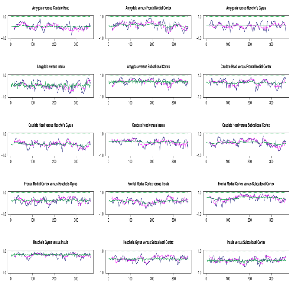
The data analysis presented in this subsection was mainly to illustrate the performance of the different estimation methods for dynamic correlation. Since the data presented originated from only one subject, not much can be read, interpreted or generalized from the results. Nevertheless, the highest correlation occurred between Heschel’s gyrus and insula (see Table 3 for the mean absolution correlation across all time points for all pairwise analyses and Table A1 in the Appendix for the corresponding maximum of absolute values of the correlations). Heschel’s gyrus contains the primary auditory cortex (PAC), the first cortical structure to process incoming auditory information [23]. In turn, PAC is in close proximity to the posterior insular cortex [23], to which it is also directly connected [24]. If we use the estimate of dynamic correlation as a proxy measure of functional connectivity, the data would imply that the Heschel’s gyrus and insula are functionally interconnected. This conclusion has clinical relevance because reduction in the functional connectivity between PAC and insula has been linked to prosody dysfunction in patients with schizophrenia [25].

Table 3. Results from Stroop data analysis
Mean of absolute value of correlations across time
	SW	WVGA	DCC1	DCC2
Amygdala vs. Caudate Head	$0.075$	$0.031$	$1.000$	$0.069$
Amygdala vs. Frontal Medial Cortex	$0.210$	$0.173$	$1.000$	$0.169$
Amygdala vs. Heschel’s Gyrus	$0.138$	$0.117$	$1.000$	$0.129$
Amygdala vs. Insula	$0.022$	$-0.020$	$1.000$	$0.047$
Amygdala vs. Subcallosal Cortex	$0.417$	$0.378$	$1.000$	$0.394$
Caudate Head vs. Frontal Medial Cortex	$0.280$	$0.301$	$1.000$	$0.299$
Caudate Head vs. Heschel’s Gyrus	$0.010$	$0.039$	$1.000$	$0.025$
Caudate Head vs. Insula	$0.214$	$0.223$	$1.000$	$0.240$
Caudate Head vs Subcallosal Cortex	$0.174$	$0.155$	$1.000$	$0.149$
Frontal Medial Cortex vs. Heschel’s Gyrus	$0.219$	$0.275$	$1.000$	$0.254$
Frontal Medial Cortex vs. Insula	$0.151$	$0.179$	$1.000$	$0.165$
Frontal Medial Cortex vs. Subcallosal Cortex	$0.440$	$0.501$	$1.000$	$0.474$
Heschel’s Gyrus vs. Insula	$0.619$	$0.622$	$1.000$	$0.656$
Heschel’s Gyrus vs. Subcallosal Cortex	$0.274$	$0.313$	$1.000$	$0.261$
Insula versus Subcallosal Cortex	$0.142$	$0.142$	$1.000$	$0.105$

LFP data analysis

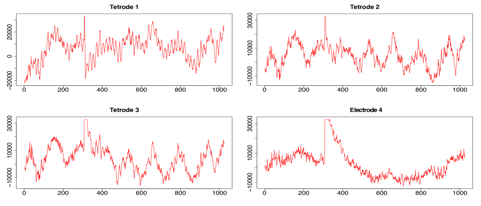
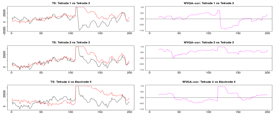
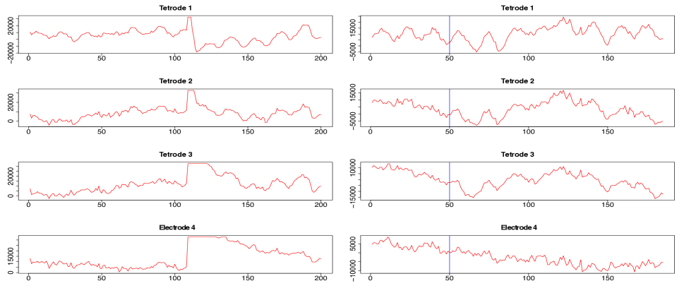
Time series corresponding to $~{}1$ second (1024 data points) from the three tetrodes and one single wire electrode are plotted in Appendix Figure A3. Tetrodes 1, 2 and 3 were placed in the CA1 field of the hippocampus, while electrode 4 was located in the medial dorsal striatum. All hippocampal tetrodes recorded a theta oscillation (7-14Hz) typical for this brain area. Signals on tetrodes 2 and 3 were most similar, and included, along with theta, oscillations of much higher frequency; these oscillations were missing in the signal recorded on tetrode 1. The signal on electrode 4, recorded in the medial dorsal striatum, lacked the theta rhythm and was visibly different from the other three LFP’s. However, in all four recordings a large jump (that is, an extreme value) corresponding to a movement artifact occurred approximately near the 300th time point. The configurations of the four signals were used to evaluate the performance of SW, DCC, and nonparametric WVGA methods discussed above. To estimate the dynamic correlations between the signals in the presence of extreme values, we cut out segments of data between time points 200 and 400 for each of the four time series (left panels of Figure 9). We expected to obtain high correlations between all segments around the 300th data point, where the movement artifact registered in all four recordings. Outside of this point, we expected high correlation between LFPs 2 and 3, somewhat lower correlation between LFP 1 and either LFP 2 or LFP 3, and low correlations between LFP 4 and the signals on any of the three tetrodes. Furthermore, because of the presence of extreme values, we also expected that our nonparametric WVGA would generate the best estimate.

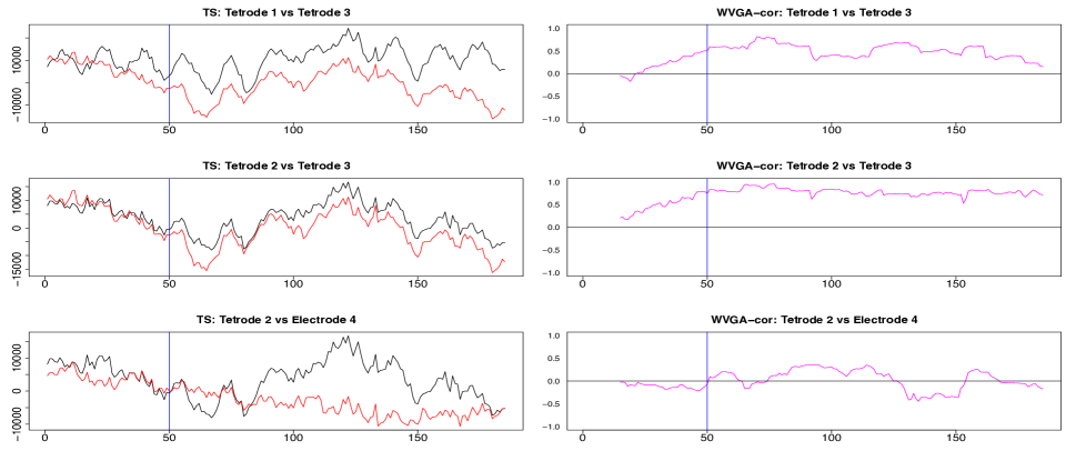
Second, we also cut segments between time points 415 and 600 (plotted in the right panels in Figure 9). Visual inspection suggested a change in signal configuration around the 50th point of these fragments which should be reflected in changes in the dynamic correlations among LFPs 1-3 (left vs. the right of the 50th time point in Figure 9, right panels). At the same time, we expected little correlation between any of the LFPs 1-3 on one hand and LFP 4 on the other hand.

Figure 9: Segments of LFP time series from four electrodes implanted in the CA1 field of the hippocampus (tetrodes 1-3) and medial dorsal striatum (electrode 4) in the brain of the same rat. Left column: Segments between time points 200 and 400 from the respective time series plotted in appendix figure A3. Right column: segments between time points 415 and 600 of time series seen in figure A3. $50^{th}$ time point within these segments is marked by a blue vertical line.

The results from pairwise analyses of dynamic correlations for the segments in the left side of figure 9 are plotted in figure 10. In all these plots, the estimates generated by the SW and DCC methods fluctuated rapidly compared to nonparametric WVGA, suggesting that the presence of extreme values affected SW and DCC much more than WVGA. As in the fMRI analysis, the two DCC estimates based on the two different R packages differed markedly. Moreover, the SW method did not always result in a correlation value (see discontinuities in the blue curve in Figure 10) because in some portions the original signals consisted of series of equal numbers with zero standard deviation. Thus, the WVGA method generated the best estimates for this set of time series.

Visual comparison of LFPs 1 and 3 (first and third right panels in Figure 9, top left panel in Figure A4) indicated that although both signals were dominated by the theta rhythm and showed a movement artifact, they were overall dissimilar, particularly at the later time points. The WVGA estimates (top right in Figure 10, top right in Figure A4) reflected accurately these variations, showing low correlation at the beginning of the signals that raised to a maximum correlation at the point of the extreme values corresponding to the movement artifact, dipped to negative values in the immediate aftermath of the peaks, and returned to positive values at the very end. Similarly, visual inspection of the tetrodes 2 and 3 signals (middle two panels in the left side of Figure 9; middle left panel in Figure A4), suggested consistent high correlations across all time points within the segments. The results of the nonparametric WVGA analysis showed that this was indeed the case (magenta curve in the middle right panel of Figure 10; middle right panels of Figure A4). There was no significant dynamic shift for the magenta curve and its values were above 0.5 for a significant portion of the segment. In contrast, the other estimates fluctuated rapidly (blue and green curves, middle right panel in Figure 10) which neither makes sense biologically, nor verifies our understanding based on visual inspection of the original pair of LFPs. Finally, the WVGA estimate indicated that the dynamic correlation between any of the hippocampal signals (LFPs 1-3) and the striatal signal (LFP4) was consistently low except in the section of extreme values, where, not surprisingly, the values were high (middle and bottom right, bottom left in Figure 10, bottom right in figure A4). This assessment corresponded with our expectation that the LFPs originating in the two different brain areas would be uncorrelated.

Figure 10: Pairwise dynamic correlations for time series plotted in the left column panels in figure 9. Blue (SW), green solid (DCC with rmgarch), green dashed (DCC with ccgarch), and magenta (WVGA).

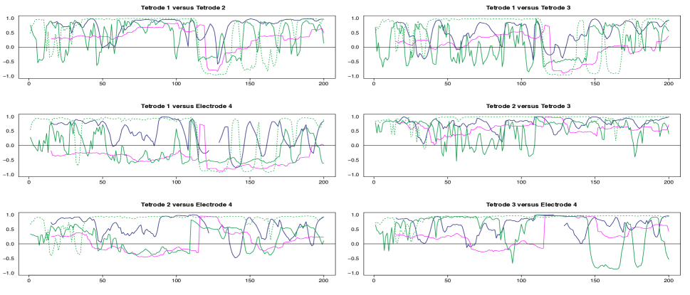
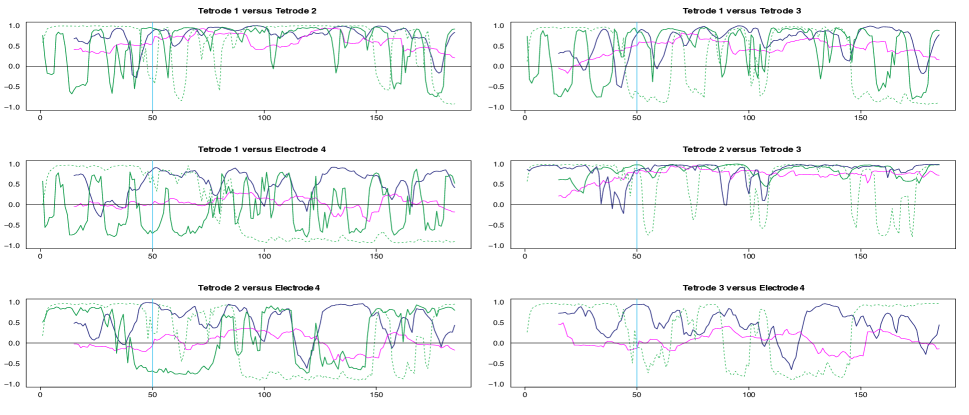
The results from pairwise analyses of dynamic correlations for the segments in the right side of Figure 9 are plotted in Figures 11 and A5. As previously, the estimates based on SW and DCC fluctuated rapidly and the two DCC-based estimates differed significantly in all cases, even for the LFPs 2 and 3, which were very similar. In contrast, WVGA analysis reflected correctly the switch in dynamic correlation before and after the 50th time point and the higher similarity between the signals on tetrodes 2 and 3 vs. signal on tetrode 1 (top left panel and top two right panels in Figure 11, top two rows in Figure A5). Except for the segment before the 50th point, the nonparametric WVGA estimate of the dynamic correlation between tetrodes 2 and 3 was consistently above 0.5, confirming our visual evaluation. The estimate for the same time points of the dynamic correlations of electrode 1 with electrodes 2 and 3, respectively, showed near zero values in the beginning that gradually rose and after the $50^{th}$ time point, the values were mostly above 0.5. These results again confirmed our visual observation of the original time series. Finally, as expected, the nonparametric WVGA estimates of dynamic correlations between hippocampal and striatal LFPs were near zero for most of the time points. Thus, the nonparametric WVGA method led to meaningful results.

Figure 11: Pairwise dynamic correlations for time series plotted in the right column panels in figure 9. Blue (SW), magenta (WVGA), green solid (DCC with rmgarch) and green dashed (DCC with ccgarch). $50^{th}$ time point within these segments is marked by a light blue vertical line. The green dashed curve in the lower right panel is missing, indicating a convergence problem with the DCC with ccgarch in this case.

Discussion and Conclusions

Understanding the dynamic correlation underlying a pair of time series is of interest in many areas including neuroscience. Currently, existing techniques such as sliding window (SW) or GARCH-based DCC can be applied to this estimation problem. Linquist and co-authors[8] evaluated the existing methods and concluded that DCC is an attractive option for effective dynamic correlation estimation in fMRI data. Our analysis confirmed that DCC performs well for nicely behaved time series from a bivariate normal distribution. However, for time series with extreme values, common in neuroscience, DCC performs much more poorly. To address this problem, we propose a nonparametric approach to the estimation of dynamic correlation by adapting the weighted visibility graph algorithm, a relatively novel method introduced by physicists [11,16, 17, 26] that converts a time series into a graph. This method is independent from finite moment assumptions, rendering it robust to extreme values.

To study how the nonparametric WVGA compares with the SW and DCC methods, we conducted extensive simulations as in Lindquist et al [8]. We also compared the results obtained by applying the three methods to one real fMRI data set and to one LFP data set with known properties and extreme values recorded in an awake rat. These analyses indicated that the WVGA based method led to more biologically meaningful results and performed better in the presence of outliers than SW or DCC.

We also found that both in the simulations and in the analysis of the fMRI data set, DCC exhibited convergence problems. We speculate that these issues are possibly generated by the optimization algorithms involved. The state-of-the-art method for estimating the parameters in the DCC model uses a 2-stage ML method involving numerical optimization, a procedure whose routines may exhibit convergence issues - non-convergence, or convergence to the wrong solutions. Convergence problems do not exist for WVGA based method because it does not involve the estimation of any parameters.

The nonparametric WVGA method performs very well in the scenarios for which it was intended to be utilized, but a deeper understanding of this performance remains to be yet developed. Our adaptation of WVGA is a bit ad-hoc in nature, unlike, for example, DCC, which is based on well-established statistical frameworks such as GARCH and quasi-likelihood estimation. One factor that may contribute to the optimal performance of the nonparametric WVGA method could be the combination of local and global aspects of its algorithm. Method $\#1$ (SW) is based on only local information - correlation at each time point is based only on the values within the sliding window. As mentioned in Lindquist et al [8], in these conditions the dynamic profiles of even random noise may show compelling changes in correlation across time. The local nature of SW could be transformed into a more global nature by increasing the window-size, but increasing the window-size beyond a particular level will lead to the method overlooking real dynamic changes. Method $\#2$ is much more of a global estimation approach. In DCC, only the parameters of the covariance/correlation matrix are considered to vary while all other parameters ($\omega_{1},\alpha_{1},\beta_{1},\omega_{2},\alpha_{2},\beta_{2}$ in Lindquist et al’s notation) remain constant. The new approach based on WVGA incorporates both local and global components. Since it is window-based, it is partly local in nature like SW. However, for time points within each window the correlations calculated involve median weight vectors with similar length as that of the original time series and consisting of weights from all time points from the entire series. This approach confers global character to the new method. The combined local and global aspects of the nonparametric WVGA method may result in optimal performance on data sets that do not conform to normality and contain extreme values. While this aspect remains to be explained in more detail through further work, it is clear that extreme values do not pose a problem for our nonparametric WVGA, which is based on a weighted graph where the weights are calculated using an arctan function. arctan, like other functions used in robust estimation such as Huber’s function, trimming function or Tukey’s bisquare function reduces the influence of outlying values by applying a cap (see section 14.5 in [27]). In contrast, DCC, like most other parametric methods, is influenced disproportionately by the extreme values.

Although the ad hoc nature of our adaptation of WVGA is not a limitation per se because the method performs well in practice, gaining a deeper understanding of why it works would facilitate improving the current version presented in this paper. Visibility graphs other than the one utilized in this paper have been discussed in the literature, the most prominent among them being the horizontal visibility graph. Future work will include exploring the performance of adaptations of these alternate visibility graph algorithms for estimating dynamic correlation.

References

Appendix

Figure A1: The green curves (DCC estimates) in the bottom panel of figure 1, with $y$-axis zoomed in, to see that the curves are not really straight lines.

Figure A2: The time series plot in the top panel in figure 2, with the $y$-axis margins expanded.

Table A1. Results from Stroop data analysis
Maximum of absolute value of correlations across time
	SW	WVGA	DCC1	DCC2
Amygdala vs. Caudate Head	$0.823$	$0.507$	$1.000$	$0.194$
Amygdala vs. Frontal Medial Cortex	$0.882$	$0.666$	$1.000$	$0.347$
Amygdala vs. Heschel’s Gyrus	$0.657$	$0.504$	$1.000$	$0.129$
Amygdala vs. Insula	$0.767$	$0.584$	$1.000$	$0.555$
Amygdala vs. Subcallosal Cortex	$0.830$	$0.692$	$1.000$	$0.674$
Caudate Head vs. Frontal Medial Cortex	$0.795$	$0.701$	$1.000$	$0.467$
Caudate Head vs. Heschel’s Gyrus	$0.606$	$0.492$	$1.000$	$0.254$
Caudate Head vs. Insula	$0.736$	$0.602$	$1.000$	$0.362$
Caudate Head vs Subcallosal Cortex	$0.800$	$0.624$	$1.000$	$0.280$
Frontal Medial Cortex vs. Heschel’s Gyrus	$0.757$	$0.629$	$1.000$	$0.461$
Frontal Medial Cortex vs. Insula	$0.789$	$0.684$	$1.000$	$0.302$
Frontal Medial Cortex vs. Subcallosal Cortex	$0.886$	$0.831$	$1.000$	$0.597$
Heschel’s Gyrus vs. Insula	$0.892$	$0.851$	$1.000$	$0.799$
Heschel’s Gyrus vs. Subcallosal Cortex	$0.817$	$0.703$	$1.000$	$0.419$
Insula versus Subcallosal Cortex	$0.693$	$0.599$	$1.000$	$0.311$

Figure A3: LFP time series related to two consecutive time stamps (1024 data points sampled at 1KHz, approximately 1 sec) from four tetrodes. From each of these time series, segments between time points 200 and 400, and between 415 and 600 were cut out and plotted in left and right panels, respectively, of figure 9. These segments were analyzed for illustrating the dynamic correlation estimation methods.

Figure A4: Three plots selected from the pairwise plots in Figure 10. LFP pairs are shown in the left column, the resulting dynamic correlations computed by using the nonparametric WVGA method are shown in the right column. In all cases, the maximum correlation occurs at the time point corresponding to the stimulus artifact. Overall, the highest correlations resulted for the tetrodes 2 and 3 LFPs which are the most similar, while the dynamic correlation between the very different LFPs of tetrode 2 and electrode 4 were dominated by low values.

Figure A5: Three plots selected from the pairwise plots in Figure 11. LFP pairs are shown in the left column, the resulting dynamic correlations computed by using the nonparametric WVGA method are shown in the right column. The hippocampal LFPs become more similar after the 50th time point and the dynamic correlations in the top two panels reflect adequately this change. The LFP’s recorded in hippocampus and medial dorsal striatum are very different, a characteristic reflected in the low values of the corresponding dynamic correlation.

References

- [1] Allen, E.A., Damaraju, E., Plis, S.M., Erhardt, E.B., Eichele, T., Calhoun, V.D., 2012. Tracking whole-brain connectivity dynamics in the resting state. Cereb. Cortex. http://dx.doi. org/10.1093/cercor/bhs352.
- [2] Chang, C., Glover, G.H., 2010. Time–frequency dynamics of resting-state brain connectivity measured with fMRI. Neuroimage 50 (1), 81–98.
- [3] Cribben, I., Haraldsdottir, R., Atlas, L.Y., Wager, T.D., Lindquist, M.A., 2012. Dynamic connectivity regression: determining state-related changes in brain connectivity. Neuroimage 61 (4), 907–920.
- [4] Handwerker, D.A., Roopchansingh, V., Gonzalez-Castillo, J., Bandettini, P.A., 2012. Periodic changes in fMRI connectivity. Neuroimage 63, 1712–1719.
- [5] Hutchison, R.M., Womelsdorf, T., Allen, E.A., Bandettini, P.A., Calhoun, V.D., Corbetta, M., Penna, S.D., Duyn, J., Glover, G., Gonzalez-Castillo, J., et al., 2013. Dynamic functional connectivity: promises, issues, and interpretations. NeuroImage 80, 360–378.
- [6] Jones, D.T., Vemuri, P.,Murphy,M.C., Gunter, J.L., Senjem, M.L.,Machulda, M.M., Przybelski, S.A., Gregg, B.E., Kantarci, K., Knopman, D.S., et al., 2012. Non-stationarity in the “resting brain’s” modular architecture. PLoS One 7 (6), e39731.
- [7] Kiviniemi, V., Vire, T., Remes, J., Elseoud, A.A., Starck, T., Tervonen, O., Nikkinen, J., 2011. A sliding time-window ICA reveals spatial variability of the default mode network in time. Brain Connectivity 1 (4), 339–347.
- [8] Lindquist, M.A., Xu, Y., Nebel, M.B., Caffo, B.S., 2014. Evaluating dynamic bivariate correlations in resting-state fMRI: A comparison study and a new approach. NeuroImage 101 531-546.
- [9] Engle, R., 2002. Dynamic conditional correlation: a simple class of multivariate generalized autoregressive conditional heteroskedasticity models. J. Bus. Econ. Stat. 20 (3), 339–350.
- [10] Engle, R.F., Sheppard, K., 2001. Theoretical and empirical properties of dynamic conditional correlation multivariate Garch. Technical Report. National Bureau of Economic Research.
- [11] Lacasa, L., Luque, B., Ballesteros, F., Luque, J., and Nuno, J.C. (2008) From time series to complex networks: The visibilty graph. Proc. Natl. Acad. Sci. USA 105, 13, 4972-4975.
- [12] Purdon, P.L., Solo, V., Weisskoff, R.M., Brown, E.N., 2001. Locally regularized spatiotemporalmodeling and model comparison for functional MRI. Neuroimage 14 (4), 912–923.
- [13] Bollerslev, T., 1986. Generalized autoregressive conditional heteroskedasticity. J. Econ. 31 (3), 307–327.
- [14] Francq, C., Zakoian, J-M., 2010. GARCH Models: Structure, Statistical Inference and Financial Applications. Wiley. ISBN: 978-0-470-68391-0
- [15] Ye, Y., 1988. Interior algorithms for linear, quadratic, and linearly constrained non linear programming, PhD Thesis, Department of EES Stanford University, Stanford CA.
- [16] Supriya, S., Siuly, S., Wang, H., Cao. J. and Zhang, Y., 2016. Weighted visibility graph with complex network features in the detection of epilepsy, IEEE Access. Volume 4. Pages 6554 - 6566.
- [17] Zhang, J., Small, M., 2006. Complex network from pseudoperiodic time series: Topology versus dynamics, Phys. Rev. Lett., vol. 96, no. 23, p. 238701, Jun. 2006.
- [18] Stroop, J.R., 1935. Studies of interference in serial verbal reactions. J Exp Psychol XVIII: 643-662.
- [19] Verstynen, T.D. 2014. The organization and dynamics of corticostriatal pathways link the medial orbitofrontal cortex to future behavioral responses. J Neurophysiol. 2014 Nov 15;112(10):2457-69. doi: 10.1152/jn.00221.2014. PubMed PMID: 25143543.
- [20] Legatt, A.D., Arezzo, J., Vaughan H.G., Jr., 1980. Averaged multiple unit activity as an estimate of phasic changes in local neuronal activity: effects of volume-conducted potentials. Journal of neuroscience methods. 2 (2): 203–17.
- [21] Gray, C.M., Maldonado, P.E., Wilson, M., McNaughton, B., 1995. Tetrodes markedly improve the reliability and yield of multiple single-unit isolation from multi-unit recordings in cat striate cortex. Journal of neuroscience methods. 63 (1-2): 43–54
- [22] Kiparizoska, S., Ikuta, T., 2017. Disrupted Olfactory Integration in Schizophrenia: Functional Connectivity Study. The International Journal of Neuropsychopharmacology, 20 (9), 470-746. DOI:10.1093/ijnp/pyx045.
- [23] Palaniyappan L, Liddle PF (2012) Does the salience network play a cardinal role in psychosis? An emerging hypothesis of insular dysfunction. J Psychiatry Neurosci 37: 17±27. doi: 10.1503/jpn.100176 PMID: 21693094
- [24] Pang, L., Kennedy, D., Wei, Q., Lv, L., Gao, J., Li, H., Quan, M., Li, X., Yang, Y., Fan, X., Song, X., 2017. Decreased Functional Connectivity of Insular Cortex in Drug Naïve First Episode Schizophrenia: In Relation to Symptom Severity PLoS ONE 12(1): e0167242. doi:10.1371/journal.pone.0167242
- [25] Leitman, D.I., Hoptman, M.J., Foxe, J.J., Saccente, E., Wylie, G.R., et al. 2007. The neural substrates of impaired prosodic detection in schizophrenia and its sensorial antecedents. Am J Psychiatry 164: 474-482. doi: 10.1176/ajp.2007.164.3.474 PMID: 17329473
- [26] Nunez, A., Lacasa, L., Luque, B. (2012) Visibility algorithms: a short review. Graph Theory (edited by Intech), ISBN 979-953-307-303-2.
- [27] Pawitan, Y. 2013. In All Likelihood. Oxford University Press; 1 edition