Phase curves of WASP-33b and HD 149026b and a New Correlation Between Phase Curve Offset and Irradiation Temperature

Abstract

We present new 3.6 and 4.5 µm Spitzer phase curves for the highly irradiated hot Jupiter WASP-33b and the unusually dense Saturn-mass planet HD 149026b. As part of this analysis, we develop a new variant of pixel level decorrelation that is effective at removing intrapixel sensitivity variations for long observations ($>$10 hours) where the position of the star can vary by a significant fraction of a pixel. Using this algorithm, we measure eclipse depths, phase amplitudes, and phase offsets for both planets at 3.6 µm and 4.5 µm. We use a simple toy model to show that WASP-33b’s phase offset, albedo, and heat recirculation efficiency are largely similar to those of other hot Jupiters despite its very high irradiation. On the other hand, our fits for HD 149026b prefer a very high albedo and an unusually high recirculation efficiency. We also compare our results to predictions from general circulation models, and find that while neither planet matches the models well, the discrepancies for HD 149026b are especially large. We speculate that this may be related to its high bulk metallicity, which could lead to enhanced atmospheric opacities and the formation of reflective cloud layers in localized regions of the atmosphere. We then place these two planets in a broader context by exploring relationships between the temperatures, albedos, heat transport efficiencies, and phase offsets of all planets with published thermal phase curves. We find a striking relationship between phase offset and irradiation temperature–the former drops with increasing temperature until around 3400 K, and rises thereafter. Although some aspects of this trend are mirrored in the circulation models, there are notable differences that provide important clues for future modeling efforts.

1. Introduction

The Spitzer Space Telescope was designed and constructed prior to the discovery of the first transiting exoplanet, but it has nevertheless become an important tool in the study of exoplanet atmospheres. In particular, the development of techniques to correct instrumental systematics and derive precise timeseries photometry from Spitzer data has enabled the first measurements of thermal emission from a diverse array of exoplanets (Seager & Deming, 2010). These measurements, in the form of secondary eclipses and phase curves, allow us to characterize the temperatures, albedos, heat transport efficiencies, and phase offsets of these planets (e.g., Cowan & Agol, 2011). For planets with observations at multiple wavelengths we can also constrain their atmospheric compositions, investigate their vertical pressure-temperature profiles, and probe the presence of clouds (Burrows et al., 2010). These Spitzer phase curves provide invaluable information about the fundamental physical processes that drive the atmospheric circulation patterns of these tidally-locked planets, and can be compared to predictions from general circulation models (GCMs; e.g., Heng & Showman, 2015). Although both models and observations are generally in good agreement on the dayside emission spectra of hot Jupiters, there are significant discrepancies in the measured night-side spectra (e.g. Zellem et al., 2014) and models that provide a good match to the measured phase curve amplitude and phase offset in a single bandpass often have difficulties matching phase curve data for the same planet at additional wavelengths (i.e. Knutson et al., 2012). This suggests that there are aspects of the atmospheric circulation, cloud properties, magnetic fields, and chemistry of these planets that are not adequately captured in current GCMs. The GCMs we use in this paper, for example, neglect clouds, magnetohydrodynamics, and disequilibrium chemistry, although some of these topics have been investigated in more focused modeling studies (e.g., Cooper & Showman 2005; Parmentier et al. 2016; Rogers 2017).

In this paper, we examine multi-wavelength phase curve observations for two planets with unusual characteristics as compared to the broader sample of transiting hot Jupiters. WASP-33b is a 2.2 M_J planet with a radius of 1.5 R_J orbiting a 1.5 M_sun $\delta$ Scuti star with a period of 1.22 days (Lehmann et al., 2015). With an irradiation temperature ($T_{0}=T_{\rm eff}/\sqrt{a_{*}}$) of 3890 K, this planet is one of the most highly irradiated hot Jupiters currently known. The star itself has pulsations at a variety of frequencies, with the dominant mode at 21 d^-1. These pulsations have an amplitude of roughly 1 mmag, about 1/4 that of the secondary eclipse depth (von Essen et al., 2014). Previous authors have measured broadband thermal emission from WASP-33b’s dayside at a variety of wavelengths, including 0.91 µm (Smith et al., 2011), 1.05 µm (von Essen et al., 2015), 2.14 µm (Deming et al., 2012; de Mooij et al., 2013), and Spitzer’s 3.6 and 4.5 µm bands (Deming et al., 2012). von Essen et al. (2015) summarize these results and combine them to obtain an average dayside brightness temperature of $3358\pm 165$ K. More recently, Haynes et al. (2015) reported evidence for a temperature inversion in the 1.1–1.6 µm dayside spectrum of this planet, and Nugroho et al. (2017) used a cross-correlation technique to detect TiO in the 0.62–0.88 µm dayside spectrum with the High-Dispersion Spectrograph on Subaru. It has long been suggested (Hubeny et al., 2003; Fortney et al., 2008; Burrows et al., 2008) that additional opacity from molecules such as gas-phase TiO and VO could lead to the formation of temperature inversions in the most highly irradiated atmospheres, and this indeed appears to be the case for WASP-33b.

Atmospheric circulation models generally predict that more highly irradiated planets should have larger day-night temperature contrasts. According to Showman & Guillot (2002), the day-night temperature difference can be thought of as resulting from a competition between the radiative cooling timescale $\tau_{rad}$ and the timescale of advection by wind, $\tau_{adv}$. Because the radiative timescale decreases much faster with increasing temperature than the advective timescale, more highly irradiated planets should have steeper day-night temperature gradients. Perez-Becker & Showman (2013) and Komacek & Showman (2016) show that the full picture is more complicated, but the general idea is still that radiation outcompetes other heat transport mechanisms for the most highly irradiated planets, causing a larger day-night temperature difference. The typical pressure at whic incident starlight is absorbed is also important for atmospheric circulation, and the presence of a dayside temperature inversion will therefore also affect the redistribution of energy to the planet’s night side (Showman et al., 2009; Lewis et al., 2014).

HD 149026b is a 0.36 M_J planet with a radius of 0.65 R_J, and orbits a subgiant G0 IV star of metallicity [Fe/H] = 0.36 with a period of 2.9 days (Sato et al., 2005). Its small radius and correspondingly large density suggest the presence of a large heavy-element core. Dodson-Robinson & Bodenheimer (2009) summarize the many attempts to estimate the mass of this core, concluding that plausible estimates range from 45-110 $M_{\earth}$, corresponding to 39-96% of total mass. Given the high metallicity of the star and the planet’s large core-mass fraction, this planet seems likely to have a high atmopsheric metallicity. Although Carter et al. (2009) analyzed four spectroscopic transit observations with Hubble’s NICMOS instrument (1.1–2.0 µm), the uncertainties from these data were too high to provide useful constraints on the planet’s transmission spectrum. Stevenson et al. (2012) subsequently obtained Spitzer secondary eclipse observations at 3.6, 4.5, 5.8, 8.0, and 16 µm and found a brightness temperature of $2000\pm 60$ K at 3.6 µm and $1600-1800$ K at longer wavelengths. When they fit these data with chemical equilibrium models, they found that they preferred models with large amounts of CO and CO₂, 30$\times$ solar metallicity, no temperature inversion, and moderate heat redistribution.

Lewis et al. (2010) studied the effect of metallicity on the warm Neptune GJ436b and found that high metallicity models had equatorial jets and strong day-night temperature variations, while lower metallicity models had weak temperature variations and high latitude jets. By contributing opacity, metals raise the photosphere to a higher altitude, where atmospheric dynamics are less important and radiative cooling is more efficient. For planets with condensate cloud layers, increasing the atmospheric metallicity also increases the amount of cloud-forming material and the corresponding cloud opacity. Although most circulation models do not currently include clouds, the presence of spatially inhomogeneous cloud layers can significantly alter the shape of both optical and infrared phase curves (Parmentier et al., 2016; Heng & Demory, 2013; Shporer & Hu, 2015).

We describe our new 3.6 and 4.5 µm phase curve observations for WASP-33b and HD 149026b in Section 2 and our analysis of this data in Section 3. In Section 4 we combine a simple toy model and more sophisticated GCM simulations for each planet to interpret these observations and search for patterns in the full sample of published thermal phase curve observations. Finally we make concluding remarks in Section 5.

2. Observations

Table 1Spitzer Observation Details

Planet	$\lambda(\mu m)$	Date (UTC)	Duration (h)	Frames	Exposure time (s)	PLD Order	Aperture radius (pix)
WASP-33b	$3.6$	June 4, 2012	37.2	311,552	0.36	2	2.5
WASP-33b	$4.5$	April 11, 2012	37.2	311,680	0.36	1	2.8
HD 149026b	$3.6$	April 8, 2011	81.2	663,104	0.36	2	2.8
HD 149026b	$4.5$	April 8, 2011	81.6	663,104	0.36	3	2.6

All observations were taken with the 3.6 and 4.5 µm arrays of the IRAC instrument on Spitzer (Fazio et al., 2004) during the post-cryogenic (warm) mission. Start dates, total durations (including downlink time), AORs, and other information about the observations used in this paper are presented in Table 1. Observations were timed to begin before a secondary eclipse and end after the following secondary eclipse, and all frames were taken in subarray mode without the now-standard peak-up pointing optimization (Ingalls et al., 2012), which was implemented after these observations were executed. Due to data volume constraints the HD 149026b observations required a single downlink break near the middle of each phase curve, resulting in a 2-3 hour gap in coverage. The WASP-33b observations were executed without any breaks for downlinks.

3. Analysis

3.1. Overview

We extract a photometric timeseries for each phase curve observation using aperture photometry, then fit the data with a combined astrophysical and noise model as described in the sections below.

3.2. Photometry

Subarray images are 32x32 pixels. We estimate and subtract the sky background from each image by excluding all pixels within a radius of 12 pixels from the star, rejecting outliers using sigma clipping, and then calculating the biweight location of the remaining pixels. The biweight location is a robust and efficient statistic implemented in astropy (Astropy Collaboration et al., 2013), and we find that it gives results comparable to methods used in previous studies (Ingalls et al., 2016). For both planets, the sky background contributes less than 1% of the total flux at 3.6 µm and less than 0.5% of the total flux at 4.5 µm for our preferred apertures.

We estimate the position of the star in each image using an iterative flux-weighted centroiding method with a circular aperture of radius 3 pixels, and perform aperture photometry using the photutils module (Bradley et al., 2016) from astropy. We consider apertures with fixed radii ranging from 1.5 to 5.0 pixels in steps of either 0.1 pixels ($1.5-3.0$ pixels) or 0.5 pixels ($3.0-5.0$ pixels).

We omit the first 0.1 days of data for each data set, which is normal procedure for Spitzer analyses (Deming et al., 2015a) and removes an obvious ramp at the beginning of the observations. The HD 149026b 3.6 observations have a downlink gap in the middle, so in addition to removing 0.1 days of data from the very beginning, we also remove 0.1 days from the post-downlink segment.

3.3. Instrumental noise model

The largest flux variations in our raw Spitzer light curves are not astrophysical, but instead result from well-known intrapixel sensitivity variations combined with telscope pointing jitter (e.g., Charbonneau et al. 2005; Grillmair et al. 2012). Although there are several different approaches to correcting for these effects, pixel level decorrelation (PLD; Deming et al. 2015a) has been among the most successful to date in fits to shorter ($<$ 10 h) observations (Ingalls et al., 2016). Following the updated definition of PLD in Benneke et al. (2017), we model the light curve as:

$$L(t)=f(t)(1+m(t-t_{0}))\left(\sum_{i=1}^{9}c_{i}P_{i}(t)\right),$$ (1)

where m is the slope, $f(t)$ is the true brightness, $P_{i}(t)$ are the normalized fluxes in a $3\times 3$ pixel box centered on the position of the star, $c_{i}$ are nine coefficients giving the relative weight of each pixel, and the final two terms are meant to model temporal variations in sensitivity. In each image, we remove astrophysical flux variations by dividing the individual pixel values by the sum of the flux across all nine pixels.

(a) 3.6 µm

(b) 4.5 µm

Figure 1.— Raw photometry and $x$ and $y$ position as a function of orbital phase for HD 149026b. The top panel shows the 3.6 µm data, and the bottom panel shows the 4.5 µm data. Fluxes have been divided by the median value, and all measurements are shown binned into sets of 128 points, corresponding to a time step of 51 seconds.

(a) 3.6 µm

(b) 4.5 µm

Figure 2.— Raw photometry and $x$ and $y$ position as a function of orbital phase for WASP-33b. See Fig. 1 caption for additional information.

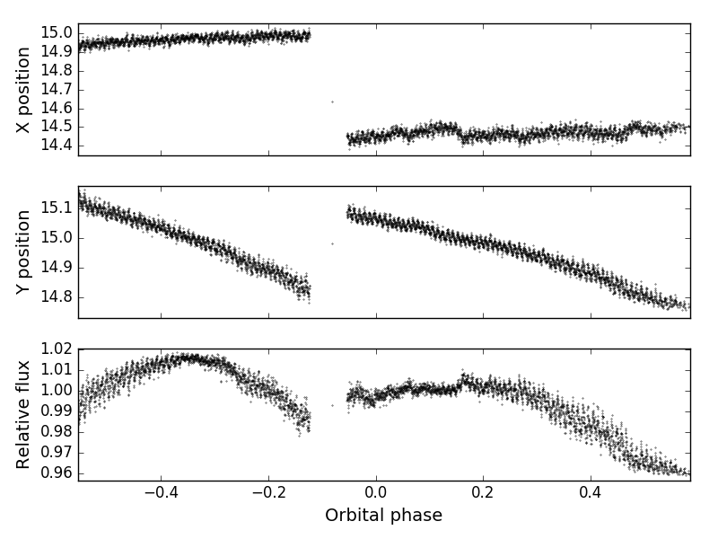
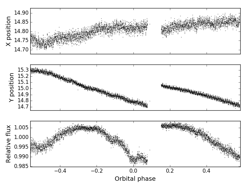
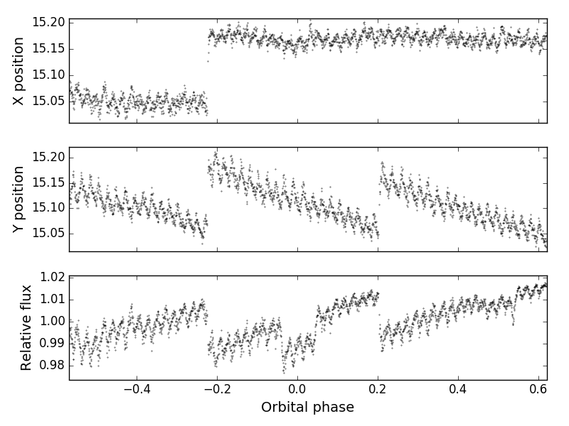
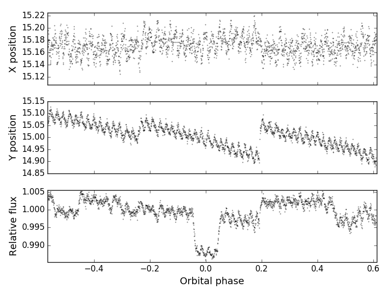
We do not necessarily expect a linear relationship between individual pixel values and the total flux across the aperture. PLD was originally formulated as the first term of a Taylor series expansion and therefore works best when applied to data where the star moves over a relatively small range (typically on the order of $1/10^{th}$ of a pixel) of pixel positions (Wong et al., 2015a). In our observations the star drifted by as much as half a pixel (see Figure 1), and we found that the standard linear PLD produced correspondingly poor fits. We account for this increased drift by developing a new variant of PLD:

$$L(t)=f(t)(1+m(t-t_{0}))\left(\sum_{i=1}^{n}\sum_{j=1}^{9}c_{ij}P_{j}(t)^{i}\right),$$ (2)

where the linear slope $m$ is a free parameter and $n$ is the highest order used in the model. This is similar to Luger et al. (2016), except that we neglect cross terms. We experimented with cross terms but found that they did not improve the quality of the fits. This, combined with the combinatorial explosion in the number of cross terms as the order is increased, convinced us to drop the cross terms.

Following Benneke et al. (2017), we have opted to include the linear term in all our fits. The inclusion of a linear term is standard in many analyses (e.g., Stevenson et al. 2012; Deming et al. 2015b) and can account for a variety of instrumental and astrophysical noise sources that are not adequately corrected by the basic instrumental noise model. We find that adding the slope decreases the value of the BIC substantially for WASP-33b’s 3.6 µm phase curve ($\Delta BIC=-34.5$) and HD-149026b’s 3.6 µm phase curve ($\Delta BIC=-15.3$), while having little effect on the value for HD 149026b 4.5 µm $(\Delta BIC=0.46)$ and increasing it for WASP-33b 4.5 µm ($\Delta BIC=7.7$). Nevertheless, we include the linear term for all light curves for uniformity. We also considered a quadratic term but found that it resulted in an increased BIC for all four visits.

We tried fits in which $n$ ranged as high as sixth order, but found that going beyond third order terms never led to lower BIC. Although we include the $m(t-t_{0})$ term in our instrumental noise model, following Deming et al. (2015a), it could also represent an astrophysical drift in the stellar brightness.

Since we use Monte Carlo Markov Chain (MCMC) to fit all parameters, one challenge is the signficant degree of degeneracy between individual pixel light curves, which can result in long convergence times for MCMC fits. We reduce these degeneracies and improve convergence times by carrying out a principle component analysis (PCA) on the $N\times 9n$ matrix of central pixel data where N is the total number of images in each phase curve observation, resulting in a $N\times 9n$ matrix of reprojected central pixel data.

3.4. Astrophysical model

Our astrophysical model consists of a transit, a secondary eclipse, and a phase curve. To model the transit and eclipse, we developed a GPU-accelerated version of batman (Kreidberg, 2015), which is roughly 10 times faster than the CPU version. This code has since been merged with the main repository. When calculating the transit and eclipse shapes we take the period from Smith et al. (2011) (WASP-33b) and Carter et al. (2009) (HD 149026b) and allow the transit timing, inclination, transit depth, eclipse depth, eclipse phase (common to both eclipses), and $a/R_{*}$ to vary as free parameters in our fits. We model the transit using a four-parameter nonlinear limb-darkening law, with coefficients derived via linear interpolation from Sing (2010). For WASP-33b, we assumed $T_{\rm eff}=7400K$, log g = 4.3, and [M/H] = 0.1 (Collier Cameron et al., 2010). For HD 149026b, we assumed $T_{\rm eff}=6160K$, log(g)=4.278, and [M/H]=0.36 (Torres et al., 2008). batman calculates the eclipse shape from geometry alone, thus neglecting limb darkening and all other sources of planetary brightness variation. Published radial velocity measurements and secondary eclipse times for both WASP-33b and HD 149026b indicate that the orbital eccentricities for both of these planets are consistent with zero (Kovács et al., 2013; von Essen et al., 2015) and we therefore fix the eccentricities of both planets to zero in our fits.

Following Cowan & Agol (2008), we model the planet’s phase variation as a series expansion in sine and cosine, where we only consider first-order sinusoidal terms:

$$L_{p}=C+c_{1}\cos(2\pi t/P)+c_{2}\sin(2\pi t/P),$$ (3)

where P is the orbital period. Although we also explored fits with second order harmonic terms, we found that these did not improve the quality of the fit for either planet.

3.5. Noise model

For HD 149206, which has a relatively quiet host star, we assume the noise is Gaussian and uncorrelated (i.e., white) and allow the value of the per-point uncertainty in each bandpass to vary as a free parameter in our fits. However, as discussed in §1, WASP-33 has quasi-periodic stellar oscillations on the order of 0.1% that need to be accounted for in order to achieve a good fit.

It is possible to model these oscillations using sinusoidal functions or wavelets, as done by other authors (i.e., Kovács et al. 2013; Deming et al. 2012; von Essen et al. 2014). However, we decided to use the Gaussian process code celerite (Foreman-Mackey et al., 2017) to fit these pulsations non-parametrically. Gaussian Processes treats the pulsations as a form of correlated noise whose properties are described by a parameterized covariance matrix fitted to our data. This avoids the need to impose a functional form on the oscillations, and allows the oscillation modes to depart from perfect periodicity over the course of the observation. We also tried using a combination of three sinusoids to fit the stellar pulsations, but found that for the WASP-33b 3.6 µm light curve, this decreased the standard deviation of the residuals by only 10%, compared to 54% for the GP code. Three sinusoids require six free parameters, as compared to the five parameters of our GP model.

celerite models the covariance matrix with a function that depends only on $\tau=|t_{i}-t_{j}|$, the time difference between two observations. We define the covariance function as the sum of two radial kernels patterned after a simple harmonic oscillator along with a diagonal kernel to represent the white noise (the latter term is functionally the same as the white noise parameter in our HD 149026 fits). The kernel $k(\tau)$ representing the correlated noise component is then:

$$k(\tau)=S_{0}\omega_{0}Qe^{-\frac{\omega_{0}\tau}{2Q}}(\cos(\eta\omega_{0}\tau)+\frac{1}{2\eta Q}\sin(\eta\omega_{0}\tau)),$$ (4)

where $\eta=|1-(4Q^{2})^{-1}|^{1/2}$. Following the recommendation of Foreman-Mackey et al. (2017), we combine two of these kernels to model the stellar variations. In the first element of our combined kernel, $Q$ is fixed to $\frac{1}{\sqrt{2}}$ while $S_{0}$ and $\omega_{0}$ are allowed to vary in our fits; this represents a non-oscillatory component that decays rapidly with $\tau$. In the second component, all three parameters are allowed to vary in order to model the oscillatory component of the stellar noise, which shows a dominant frequency of approximately 21 d^-1 in a Lomb-Scargle periodogram. We give the second $\omega_{0}$ an appropriate name: $\omega_{stellar}$. This is the parameter presented in Table 2. Our noise model thus consists of 6 parameters: $S_{0},\omega_{0}$ for the first kernel; $S_{0},Q,\omega_{0}$ for the second kernel; and a white noise term.

3.6. Markov Chain Monte Carlo Fits

We explore the parameter space for our model and determine best-fit parameters using a Markov chain Monte Carlo (MCMC) analysis. We carry out our fits using the emcee package (Foreman-Mackey et al., 2013), which is a Python implementation of an affine-invariant ensemble sampler. This approach allows for more efficient exploration of highly correlated parameters spaces, as proposed steps are generated using an ensemble of walkers whose positions are distributed along the regions of highest probability. Our models have $24-48$ free parameters, depending on planet and wavelength, so we carry out our fits using 250 walkers in order to ensure sufficient sampling of the parameter space.

We obtain a starting point for our fits by using the published transit and eclipse parameters to get a model light curve, dividing the data by the model, and obtaining PLD parameters by fitting the residuals using linear regression. For WASP-33, the Gaussian process parameters were estimated by plotting the autocorrelation and manually tweaking the parameters until we achieved a good match. We then generated initial positions for each of the 250 walkers by taking the reference values calculated above and randomly perturbing each dimension. Each dimension is first perturbed by a number drawn from a normal distribution with a mean of 0 and standard deviation of 1% of the nominal value. We then do an absolute perturbation, with each dimension being perturbed by a number drawn from a normal distribution with a mean of 0 and standard deviation of 0.01. This two-step perturbation ensures that dimensions whose initial values are 0, as well as dimensions whose initial values are far from 0, are both sufficiently spread out. Although this is a very broad distribution relative to the final uncertainties in these parameters, it ensures that our fits are able to reliably identify the global maximum in the likelihood function.

We first run emcee for 100,000 steps, resulting in a total of 25 million steps in the combined chain. We then take the single step with the highest likelihood from this chain, which should be very close to the global maximum, and initialize a new set of 250 walkers to a Gaussian ball centered around that point. The standard deviation of this ball for a given dimension is $10^{-4}$ of the initial value. We then burn in this new set of walkers and run emcee for an additional 100,000 steps. We determine our final posterior probability distributions using the last half of this chain, and confirm that the acceptance rate for this section of the chain is between 20 and 50 percent. We visually inspect the progress of randomly chosen walkers to check that there is no overall trend, and that the number of steps is appreciably larger than the period of quasiperiodic oscillations, if any. Finally, we check for convergence by calculating the average autocorrelation length for all walkers and ensure that the number of steps for each walker is at least ten times the length for each model parameter.

3.7. Model Selection and Optimization of Photometry

For each planet and each wavelength, we need to choose the optimal order ($n$ in Equation 2) for our PLD model, the photometric aperture used to generate our light curve, and the size of the bins used in the fits. As discussed in Deming et al. (2015a) and Kammer et al. (2015), the PLD method performs better when it is fit using binned light curves.

We first determine the optimal PLD order by fitting light curves generated using an aperture of 2.5 and a bin size of 128, which are representative of the optimal values in previous fits to Spitzer data sets (e.g., Wong et al. 2015b). We run MCMC fits for models with PLD orders ranging between 1 and 5. In each fit, we calculate the Bayesian Information Criterion (BIC) value (Kass & Raftery, 1995) for every position in the chain, and then calculate the median BIC over the entire chain. We then select the order with the lowest median BIC for our final version of the model. A spot check reveals that using maximum BIC instead of median BIC does not change the result.

We next choose the optimal photometric aperture by repeating our MCMC fits to photometry generated using all 20 apertures, where we fix the order of our PLD model to the optimized value and keep the same bin size as in our previous fits. In this case all of our models have the same number of free parameters, and we therefore select the aperture that produces the highest median likelihood over our MCMC chain. We also consider an alternative aperture selection metric where we compare the median (best-fit) white noise parameters for each aperture on the assumption that the best aperture should have the smallest white noise value. We find that this gives very similar results to our previously adopted likelihood metric. We list our final choice of aperture for each observation in Table 1.

The bin size is more complicated to optimize, as it represents a trade-off between minimizing the noise on short versus long timescales. If it is too big, we average over pointing variations and this can degrade the quality of the PLD model and increase the uncertainties in our model parameters. If it is too small, the PLD parameters adjust themselves in such a way as to minimize residuals on the shortest timescales ($\sim$seconds) at the expense of large timescale residuals–even though the latter is closer to the timescale of the astrophysical variations and can bias our estimates for the astrophysical model parameters. We consider bin sizes ranging from 1 to 4096 and find that a bin size of 128, corresponding to a time interval of 51 seconds, is a good compromise. 51 seconds is much longer than the shortest pointing jitter variations, which have a timescale of seconds, but much shorter than the timescale of any astrophysical signal. We therefore use 128 as the bin size for our final fits to all four phase curves.

The optimal results are presented in Table 1.

4. Discussion

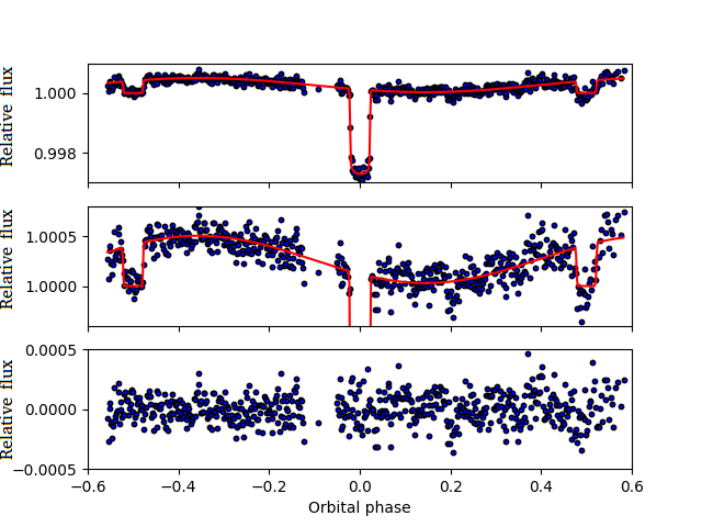
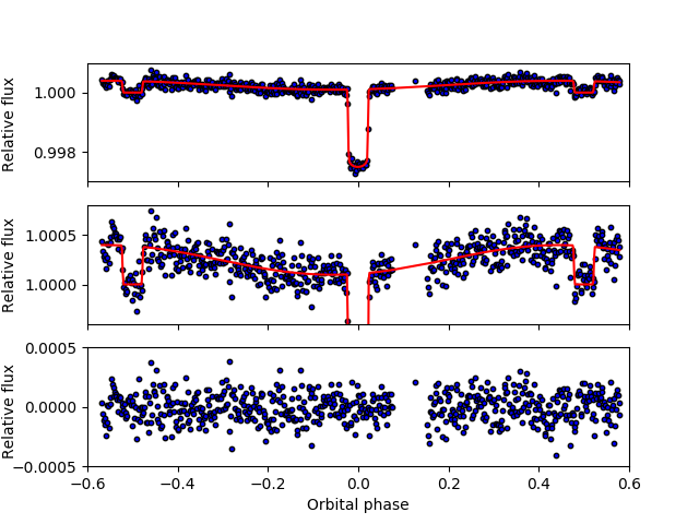
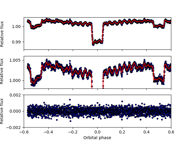
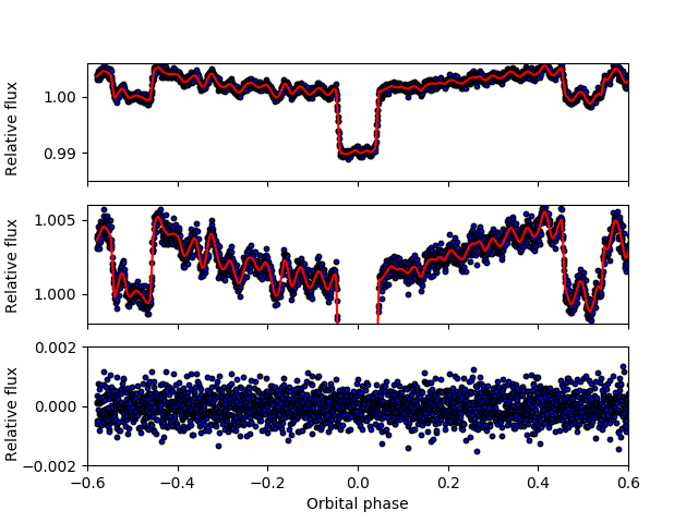
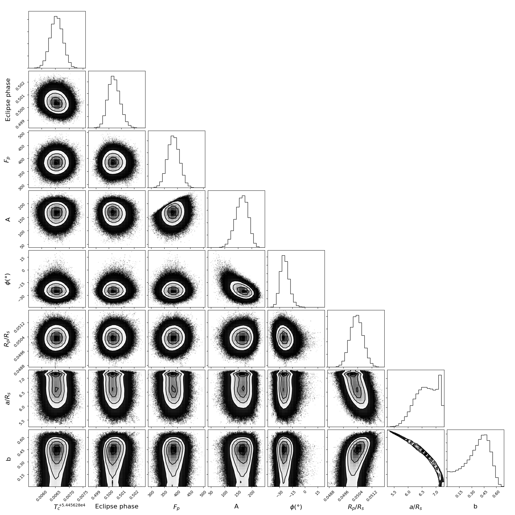
Figures 3 and 4 each show the phase curve model, the systematics-corrected observations, and the fit residuals for the highest likelihood iteration of the MCMC chain. Figure 5 shows the posterior probability distributions for our HD 149026b 4.5 µm model. The triangle plot for our HD 149026b 3.6 µm model has similar correlations, while the model parameters for WASP-33b are much more Gaussian and less correlated.

In Table 2, we present the results of our fits, including the secondary eclipse depth, phase amplitude, and phase offset at 3.6 and 4.5 µm for each planet. Here, the secondary eclipse depth ($F_{p}$) is defined as the planetary flux at the center of eclipse divided by the stellar flux. Unlike the most commonly used secondary eclipse model, which assumes that the brightness from the planet is constant over the duration of the eclipse, this model allows for variations in the planet’s brightness during this interval (see Lewis et al. 2013 for a discussion of the importance of this approach when fitting planets on highly eccentric orbits). The phase amplitude is defined as the amplitude of the sinusoidal phase curve, $A=\sqrt{c_{1}^{2}+c_{2}^{2}}$. The phase offset is the difference in degrees between the secondary eclipse center and the phase curve maximum, with a negative offset meaning the maximum occurs before the center of the eclipse.

In Table 2, we also present noise properties for each light curve. These include the measured white noise ($\sigma_{\rm white}$), the theoretical photon noise ($\sigma_{\rm photon}$), the standard deviation of the residuals of the best fit model ($\sigma_{\rm tot}$), and the lag-1 autocorrelation of said residuals–the last being a measure of correlated noise.

Table 2Best-Fit Parameters

Parameter	WASP-33b 3.6 µm	WASP-33b 4.5 µm	HD 149026b 3.6 µm	HD 149026b 4.5 µm
Eclipse depth (ppm)	$3506\pm 173$	$4250\pm 160$	$430\pm 19$	$385\pm 23$
Amplitude (ppm)	$936\pm 105$	$1792\pm 94$	$189^{+27}_{-39}$	$164^{+22}_{-24}$
$\text{Phase offset }(\degree)$	$-12.8\pm 5.8$	$-19.8\pm 3.0$	$32.2^{+17}_{-15}$	$-24.3^{+5.5}_{-4.7}$
$\text{Transit center }(\text{BJD\textsubscript{UTC}})$	$2456029.62604\pm 0.00016$	$2456024.74659\pm 0.00014$	$2455661.78488\pm 0.00021$	$2455673.28848\pm 0.00022$
$R_{p}/R_{s}$	$0.108\pm 0.001$	$0.103\pm 0.0011$	$0.0519\pm 0.0004$	$0.0503\pm 0.0004$
$a/R_{*}$	$3.65^{+0.03}_{-0.05}$	$3.65^{+0.04}_{-0.05}$	$6.38^{+0.5}_{-0.4}$	$6.67\pm 0.4$
$b$	$0.150^{+0.072}_{-0.089}$	$0.16^{+0.08}_{-0.10}$	$0.48^{+0.09}_{-0.15}$	$0.38^{+0.12}_{-0.20}$
$i$	$87.6^{+1.4}_{-1.2}$	$87.6^{+1.5}_{-1.3}$	$85.6^{+1.6}_{-1.1}$	$86.7^{+1.7}_{-1.4}$
$\phi_{\rm eclipse}$	$0.50023\pm 0.00028$	$0.50045\pm 0.00024$	$0.4989\pm 0.00033$	$0.50039^{+0.00050}_{-0.00044}$
slope (ppm/day)	$1590\pm 203$	$60\pm 170$	$510\pm 130,140\pm 100$	$-81\pm 28$
$\sigma_{\rm white}\text{(ppm)}$	$356\pm 5.6$	$451\pm 7$	$270\pm 4.4,305\pm 4.2$	$348\pm 3.6$
$\sigma_{\rm photon}\text{(ppm)}$	$306$	$411$	$227$	$313$
$\sigma_{\rm tot}\text{(ppm)}$	$628$	$708$	$290$	$347$
$\omega_{\rm stellar}\text{ (rad/day)}$	$129\pm 1.3$	$130\pm 1.5$	$-$	$-$
Lag-1 autocorrelation	$0.69$	$0.60$	$0.08$	$-0.02$

Figure 3.— Normalized light curve for our 3.6 µm (left) and 4.5 µm (right) observations of HD 149026b with our instrumental noise model divided out (blue filled circles) and a representative model fit overplotted for comparison (red line). The upper two panels show the same light curve and model with a different $y$ axis range. We show the residuals from this solution in the lower panel. All three panels use a bin size of 1024 points (6.8 minutes).

Figure 4.— Normalized light curve for our 3.6 µm (left) and 4.5 µm (right) observations of WASP-33b with the instrumental noise model divided out (blue filled circles) and a representative model, including the Gaussian Process stellar pulsation model, overplotted for comparison (red line). All three panels use a bin size of 128 points (51 seconds). See Figure 3 caption for more details.

Figure 5.— Posterior probability distributions for our fit to HD 149026b’s 4.5 µm phase curve; also known as a triangle plot. The triangle plot for HD 149026b 3.6 µm is similar, while those for WASP-33b are more Gaussian and less correlated.

4.1. Overall quality of fits and problems with the HD 149026b 3.6 µm phase curve

For every observation except HD 149026b at 3.6 µm, our higher order PLD model appears to provide a satisfactory fit to the data; as shown in Table 2, these observations have a measured white noise only 10-20% higher than the photon noise limit. As shown in Figure 3, the HD 149026b 4.5 µm observations have reasonable residuals, with no prominent unremoved systematics. WASP-33b residuals are harder to evaluate visually, but the small measured white noise indicates that most sources of error other than photon noise have been accounted for.

In contrast to the good general quality of the other light curves, the HD 149026b 3.6 µm observation should be treated with skepticism. We find that the data strongly prefer a large positive phase offset, which is inconsistent with the negative offset at 4.5 µm and is difficult to reproduce with thermal emission from standard GCMs assuming synchronous rotation (Heng & Showman, 2015).

The data themselves are of unusually low quality. This observation is divided into two segments with a 2.4 hour gap, corresponding to a telescope downlink break. In each segment the star’s position varies over an approximately oval region with a dimension of 0.5 pixels in the $x$ direction and 0.2 pixels in the $y$ direction, and the two oval regions are themselves separated by 0.5 pixels. During the first segment the star is relatively close to the center of the central pixel, but after the repointing required for the data downlink the star’s position in the second segment falls on an adjacent pixel. It is very close to the edge, with that pixel receiving 40% of the light and the second brightest pixel receiving 20%.

All of this bodes poorly for PLD correction, or for any other correction algorithm. Not surprisingly, we find that the RMS of the fit residuals for the second segment is 17% higher than in the first segment, providing tangible evidence for the persistence of these edge effects. It should be noted that none of these problems appear in the other three data sets. Both WASP-33 observations are continuous, and the star’s position shifts over an area no bigger than 0.2 by 0.2 pixels. Although the 4.5 µm observations for HD 149026 also include a downlink break in the middle, the telescope was able to return the star to approximately the same position at the end of the downlink and as a result the data from both segments span a single 0.7 x 0.2 pixel oval centered near the middle of the pixel.

We experimented with many different models for the data. We initially tried fitting the 3.6 µm HD 149026 data with a single systematics model utilizing the same $3\times 3$ pixel postage stamp centered on the middle of the array that we used for our other data sets. However, because the star is offset relative to this postage stamp during the second segment of data, this fit resulted in prominent systematics in the residuals for the second segment and a best-fit phase offset of approximately 60$\degree$. We then considered a separate Gaussian Process noise model for the two segments, where the second segment was represented by a simple harmonic oscillator kernel. The results did not change. Other models we tried including fitting only the first segment and introducing a separate linear slope for both segments.

In the end, we settled upon a separate noise and systematics model for each segment. Each segment therefore has its own PLD parameters, error parameter, and linear slope. This drastically reduced the residual systematics in the second segment. Compared to the model where both segments had the same noise and systematics model, this segmented model has 9 additional free parameters and $\Delta BIC=-926$. We found a best-fit phase offset of approximately 30$\degree$, compared to 60$\degree$ with the simpler model.

We stress that the phase offset and amplitude are likely unreliable even in this improved version of the fits. We adjusted the bin size to see what effect it has on the phase offset, and found that it monotonically decreases from 80 degrees west to 80 degrees east as the bin size increases from 1 to 4096. Similarly, the phase amplitude ranges from 190 ppm to 950 ppm, although it does not change monotonically with bin size. Although we remain concerned about the reliability of the phase curve fit in this bandpass, we conclude that the measured transit should be relatively unaffected by these structures due to its short timescale and large amplitudes. The secondary eclipse depth is somewhat more problematic. As can be seen in Figure 3, the light curve has visible systematics after the downlink break, with an upward fluctuation before the eclipse and a downward fluctuation during the eclipse. These likely bias the estimated eclipse depth. Despite this bias, we find that our 3.6 µm secondary eclipse depth is in agreement with the published value in this band from Stevenson et al. (2012).

4.2. Transit parameters and updated ephemerides

We recovered the transit time, $a/R_{*}$, $i$, and $R_{p}/R_{s}$ from the chain. The results are shown in Table 2. Notably, we do not see any of the transit anomalies seen by Kovács et al. (2013) in the WASP-33b light curves. These anomalies included a 8 mmag rise in brightness across the transit (Figure 8 of Kovács et al. 2013) and a 1.5 mmag mid-transit bump (their Figure 10), both of which were seen by multiple observers.

Table 3Updated Ephemerides for both planets

Parameter	HD 149026b	WASP-33b
Period (d)	$2.87588874$	$1.21987089$
$T_{0}(\text{BJD\textsubscript{UTC}})$	$2454456.78760$	$2454163.22367$
Error in period (d)	$5.9\times 10^{-7}$	$1.5\times 10^{-7}$
Error in $T_{0}$ (d)	$0.00016$	$0.00022$

We combined our best-fit transit times for both planets with previously published transit times to calculate updated ephemerides. For HD 149026b, we used Charbonneau et al. (2006), Winn et al. (2008), Nutzman et al. (2009), Knutson et al. (2009), Carter et al. (2009) and Stevenson et al. (2012).

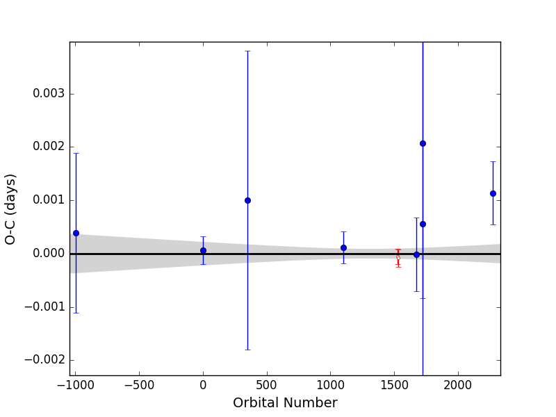
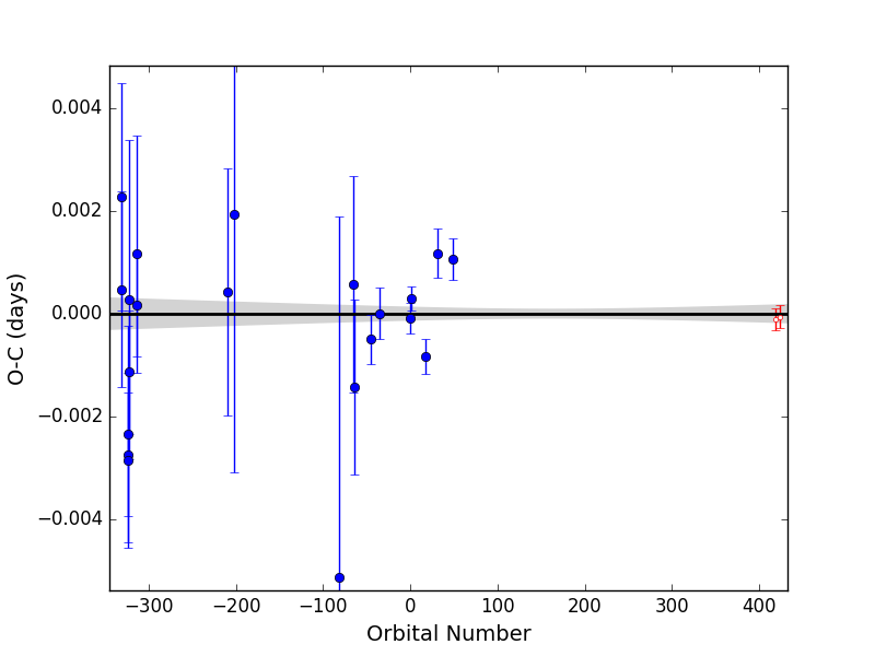
For WASP-33b, we used Collier Cameron et al. (2010), Smith et al. (2011), Kovács et al. (2013), von Essen et al. (2014), Johnson et al. (2015), and Turner et al. (2016). The updated ephemerides are shown in Table 3, and O-C plots for all transits are shown in Figure 6 and 7. We tested the goodness of fit with $\chi^{2}$, finding that both planets are consistent with a linear ephemeris–WASP-33b to well within 1$\sigma$, and HD-149026b to within 2$\sigma$ (p=0.07). For HD 149026b, both the period and transit timing are fully consistent with Carter et al. (2009). For WASP-33b, both the period and transit timing are fully consistent with Kovács et al. (2013).

It is notable that for both planets, the radius ratio is inconsistent between the two channels, differing by 3% for HD 149026b and 5% for WASP-33b. This could be due to imperfect modeling of stellar oscillations for WASP-33b, or to uncorrected systematics for both planets. The difference corresponds to roughly five atmospheric scale heights for HD 149026b and twelve scale heights for WASP-33b. Similarly large discrepancies have been reported in ground-based transit observations of other planets (e.g., Mancini et al., 2016), but these appear to be inconsistent with most model predictions as well as space-based transmission spectroscopy of similar planets (e.g., Sing et al. 2016).

Kovács et al. (2013) carried out a comprehensive analysis of ground-based WASP-33b light curves, consisting of amateur and professional data in the optical and near infrared bands. They found $R_{p}/R_{s}=0.1143\pm 0.0002$, which is a remarkable 6-10$\sigma$ higher than our Spitzer values. However, the authors note anomalies in many of their data sets, including a mid-transit hump, a skewed transit shape, and discrepancies in transit depth measurements that are much larger than the formal errors.

HD 149026b has more consistent transit depths in the literature. Winn et al. (2008) found $R_{p}/R_{s}=0.0491^{+0.0018}_{-0.0005}$ in Stromgren (b+y)/2 photometry, Nutzman et al. (2009) found $R_{p}/R_{s}=0.05158\pm 0.00077$ at 8 µm, and Carter et al. (2009) found $R_{p}/R_{s}=0.05416^{+0.00091}_{-0.00070}$ with NICMOS (1.1-2.0 µm). The last measurement is $2-3\sigma$ higher than our Spitzer values, but our results are consistent with Winn et al. (2008) and Nutzman et al. (2009).

For HD 149026b, our measured secondary eclipse depths are fully consistent with those measured by Stevenson et al. (2012) in the same Spitzer bands using BLISS mapping. For WASP-33b, the eclipse depth is in good agreement with Deming et al. (2012) at 4.5 µm, although it is $1.7\sigma$ higher at 3.6 µm. This might be because of imperfect modeling of stellar pulsations, leading to underestimated error bars in both papers. Since we have a longer observational baseline over which to characterize stellar pulsations and measured two eclipses instead of one, our measurement of the eclipse depth should be less sensitive to the effects of stellar pulsations than Deming et al. (2012).

Figure 6.— Observed minus calculated transit times for WASP-33b calculated using our updated ephemeris. Previously published results are shown as blue filled circles, and our results are shown as red open circles. The black line indicates the predicted transit times at each epoch assuming a constant ephemeris, and the gray region indicates the 1$\sigma$ confidence interval.

Figure 7.— Observed minus calculated transit times for HD 149026b calculated using our updated ephemeris; see Fig. 7 caption for more details.

4.3. Constraints on atmospheric circulation

4.3.1 General circulation models

We present cloud-free GCMs for HD 149026b and WASP-33b calculated using the Substellar and Planetary Atmospheric Radiation and Circulation (SPARC) model (Showman et al., 2009), which couples the MITgcm (Adcroft et al., 2004) to a two-stream implementation of the multi-stream, plane-parallel radiative transfer code of Marley & McKay (1999). The MITgcm is an atmospheric and oceanic circulation model that solves the primitive equations, which are relevant for stably stratified atmospheres with large horizontal/vertical aspect ratios (generally true for hot Jupiters). The equations are solved using a finite-volume discretization on a cubed-sphere grid, which allows longer time steps and increases the accuracy near the poles as compared to a traditional longitude-latitude grid. The radiative transfer code employs the correlated-k method with 11 bands optimized for accuracy and computational efficiency. The opacities are calculated assuming local thermodynamic and chemical equilibrium. This code has been used extensively to model the atmospheric circulation of exoplanets over a wide range of planetary properties (e.g., Lewis et al. 2010; Kataria et al. 2015, 2016; Wakeford et al. 2017). After running the GCM, we extract light curves following the method of Fortney et al. (2006).

We list the predicted eclipse depths, amplitudes, and phase offsets at 3.6 and 4.5 µm for each model in Table 4; these can be compared directly to the measured values in Table 2.

(a) Solar metallicity

(b) $30\times$ solar metallicity

Figure 8.— Comparison of the GCM-generated phase curves (thick lines) for HD 149026b with our measured phase curves (thin lines). The 24 thin lines each represent one randomly selected MCMC step, and the dispersion in these lines is therefore representative of the uncertainties in the measured phase curve shape. No TiO is included. 3.6 µm results are plotted as blue curves while 4.5 µm results are in red.

Table 4Phase curve parameters from GCMs

Planet	TiO?	Metallicity	Band (µm)	$F_{p}\text{(ppm)}$	A (ppm)	$\phi(\degree)$
WASP-33b	No	$1\times$	3.6	$4086$	1664	$-9.9$
WASP-33b	No	$1\times$	4.5	$4597$	1903	$-9.6$
WASP-33b	Yes	$1\times$	3.6	$4151$	1688	$-8.8$
WASP-33b	Yes	$1\times$	4.5	$4779$	1981	$-7.6$
HD 149026b	No	$30\times$	3.6	$430$	167	$-11$
HD 149026b	No	$30\times$	4.5	$616$	252	$-7$
HD 149026b	No	$1\times$	3.6	$219$	31.9	$-55$
HD 149026b	No	$1\times$	4.5	$260$	49.6	$-45$

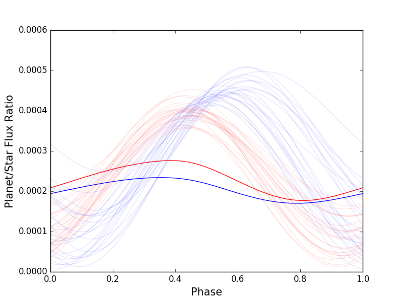
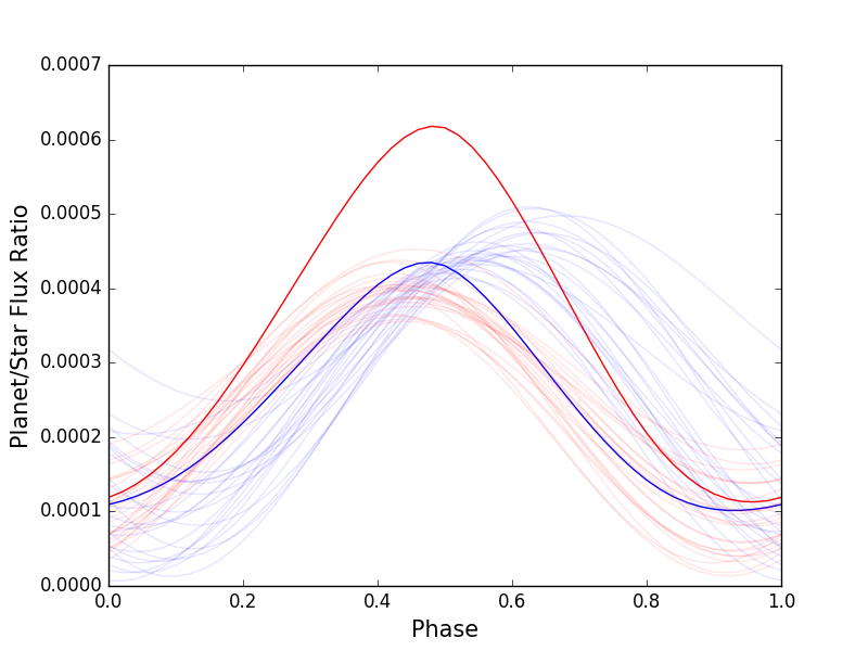
For HD 149026b we consider models with solar and $30\times$ metallicity and compare the resulting phase curves to our best-fit phase curve model in Figure 8. We only consider models without TiO, as Stevenson et al. (2012) found that this planet’s dayside emission spectrum was best described by a model without a temperature inversion. We find that the solar metallicity GCM predicts a relatively small phase curve amplitude in both bandpasses, in sharp disagreement with our data. The $30\times$ solar metallicity model has a higher opacity in both Spitzer bandpasses and therefore probes lower pressures (higher altitudes) than the solar metallicity model, leading to larger predicted phase curve amplitudes. This model comes closer to matching the data, although it underestimates the amplitude at 3.6 µm and overestimates it at 4.5 µm. We note that neither the 1D models shown in Stevenson et al. (2012) nor the 3D GCMs are able to match the measured secondary eclipse depths at 3.6 and 4.5 µm, and speculate that these discrepancies in both secondary eclipse depths and phase curve amplitudes might be resolved by increasing the amount of CO and/or CO₂ in the atmosphere. Both CO and CO₂ have absorption bands in the 4.5 µm Spitzer bandpass, increasing their abundance will accordingly decrease the planet’s brightness in this band relative to the 3.6 µm band. Previous models for GJ 436b (Moses et al., 2013; Morley et al., 2017) serve as a useful demonstration of the effect of very high atmospheric metallicities ($>200-300\times$ solar) on the strength of the CO absorption in the 4.5 µm band. On the planet’s night side, which is cool enough to fall near the transition from CO to methane-dominated carbon chemistry, disequilibrium chemistry due to quenching and horizontal transport could increase the relative amount of CO and CO₂ (Cooper & Showman, 2006).

(a) Without TiO

(b) With TiO

Figure 9.— Comparison of GCM-generated phase curves (thick lines) for WASP-33b with our measured phase curves (thin lines). The 24 thin lines each represent a randomly selected MCMC step, and the dispersion in these lines is therefore representative of the uncertainties in the measured phase curve shape. Both models assume solar metallicity. 3.6 µm results are plotted as blue curves and 4.5 µm results are in red.

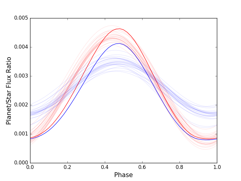
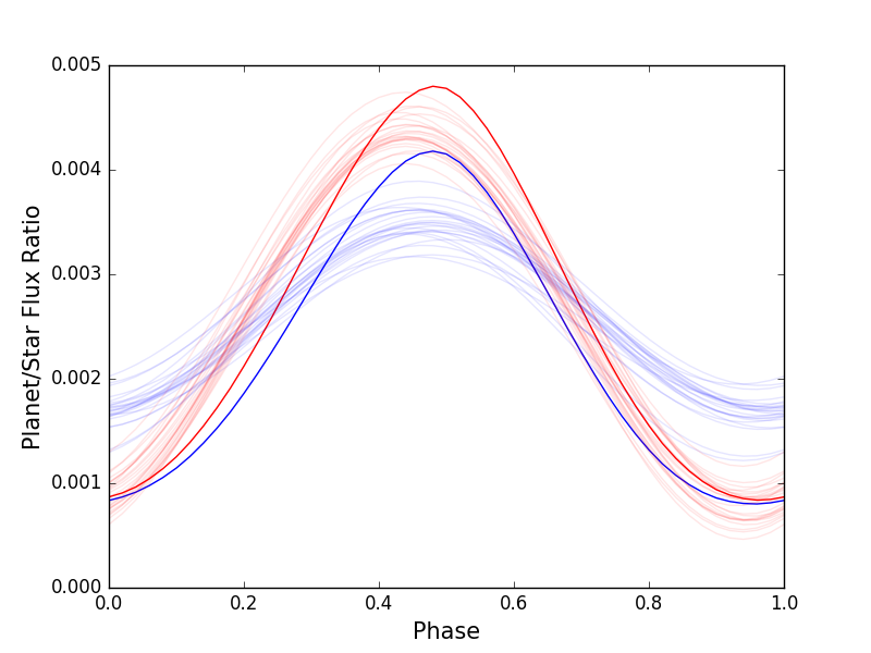
For WASP-33b, which has a much lower bulk density than HD 149026b, we consider only the solar metallicity case for our GCMs. As discussed in Section 1, this planet is one of the most highly irradiated hot Jupiters discovered to date; its dayside emission spectrum is best matched by models with a temperature inversion and appears to hint at the presence of gas-phase TiO. We show predictions for two models in Figure 9, including one with and the other without TiO, in order to evaluate the effect of this molecule on its dayside emission spectrum and day-night circulation. We find that the differences in the phase curves for these two models are fairly subtle, and although the data are somewhat better matched by the model without TiO, both models disagree with the observations at the $2\sigma$ level. In this case the models predict a larger phase curve amplitude and secondary eclipse depth in both bands.

Figure 10.— Model emission spectrum for WASP-33b, compared with observations (black filled circles for our values, black open circles for literature values from Smith et al. 2011; von Essen et al. 2015; Deming et al. 2012; de Mooij et al. 2013). Each blue or green point represents the band-averaged flux ratio corresponding to the observation at the same wavelength.

Figure 11.— Model emission spectrum for HD 149026b, compared with observations (black filled circles for our values, black open circles for literature values from Stevenson et al. (2012)). Each blue or green point represents the band-averaged flux ratio corresponding to the observation at the same wavelength.

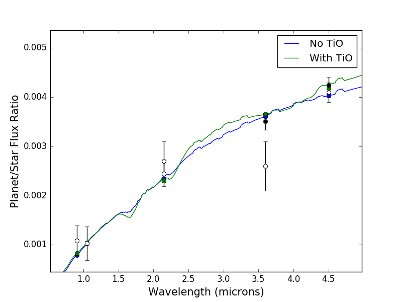
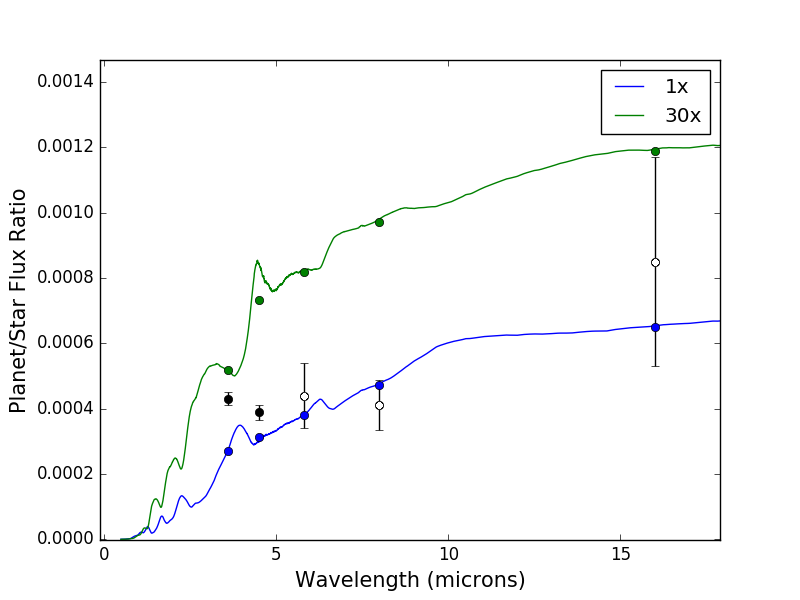
In Figure 10 and 11, we show the GCM-derived emission spectra for the two planets. Our WASP-33b observations are consistent with both GCMs, which have very similar emission spectra at Spitzer wavelengths. HD 149026b, on the other hand, is highly inconsistent with both GCMs in the Spitzer 3.6 and 4.5 µm bands. Interestingly, eclipse observations in the 5.8, 8, and 16 µm Spitzer bands seem to favor the solar metallicity model over the $30\times$ solar metallicity model. We speculate that this could be because the GCMs assume gas-only opacity with no hazes or clouds, resulting in a very low albedo; in contrast, our phase curve data appear to favor a high albedo (see discussion in Subsection 4.3.2). A high albedo would cool the planet’s dayside, bringing the 30x model into bet- ter agreement with the data. However, even with a reduced amplitude the 30x solar model is a poor match for the observed spectral slope across the 3.6-4.5 um bands; this could be explored with additional models in the future. We note that our preference for the high metallicity model is primarily driven by the need to match the large observed phase curve amplitudes in both bands rather than the shape of the planet’s dayside emission spectrum. As an alternative to changing the planet’s dayside albedo, the addition of localized clouds on the planet’s night side could increase the phase curve amplitude for the solar metallicity model (e.g., Stevenson 2016), bringing it into better agreement with our observations.

4.3.2 A simple toy model for albedo and recirculation efficiency

In this section, we use a simple toy model first presented in Cowan & Agol (2011) to calculate average brightness temperatures, albedos, and circulation efficiencies for the two planets under the assumption that their thermal emission is well-approximated by a blackbody and that these observations probe a similar range in pressures across all wavelengths and longitudes. In this model, a planet’s thermal phase curve is described by two parameters: a Bond albedo ($A_{B}$) and a heat redistribution efficiency ($\varepsilon$). Planets absorb a fraction $1-A_{B}$ of the stellar flux on their daysides, redistribute this energy to the nightside with the stated efficiency, and then emit as a blackbody. In the $\varepsilon=1$ case, the entire planet has the same temperature, and energy balance gives $T_{p}=\frac{T_{0}}{\sqrt{2}}(1-A_{B})^{1/4}$ where $T_{0}=\frac{T_{s}}{\sqrt{a_{*}}}$ and $a_{*}=\frac{a}{R_{s}}$. For the $\varepsilon=0$ case (i.e., no heat redistribution to the night side), the corresponding dayside temperature is given by $T_{d}=(2/3)^{1/4}(1-A_{B})^{1/4}T_{0}$ and the nightside temperature is zero. If we define $\varepsilon$ so that it linearly interpolates between these two extremes we arrive at an analytic description for $\varepsilon$ and $A_{B}$ as a function of the effective blackbody temperatures for the planet’s dayside ($T_{d}$) and nightside ($T_{n}$):

$$\varepsilon=\frac{8}{5+3(T_{d}/T_{n})^{4}}$$ (5)

$$A_{B}=1-\frac{5T_{n}^{4}+3T_{d}^{4}}{2T_{0}^{4}}.$$ (6)

Here, and throughout the paper, we define the nightside and dayside to mean an orbital phase of 0 and 0.5, respectively. Previous studies have alternated between this definition and one in which day and night correspond to the hottest and coldest hemispheres on the planet.

The hemisphere-averaged planet brightness temperature is given by Equation 6 in Cowan & Agol (2011), and depends on two things: the brightness temperature of the star at the observed wavelength, and the ratio $\psi(\lambda)$ between normalized planetary flux and transit depth at the observed wavelength. We first calculate the stellar brightness temperature in each band using the closest model in the BT-NextGen (AGSS2009) spectral grid, as provided by the Spanish Virtual Observatory. The spectral grid spacing is fine enough that choosing the adjacent model changes the brightness temperature by less than 1%. As a check on BT-NextGen, we also calculated brightness temperatures using Phoenix models (Husser et al., 2013), and found that the results differed on average by only 0.4%. We next calculate the planet-star brightness ratio $\psi(\lambda)$ for the day side by dividing the eclipse depth $F_{p}$ by the transit depth, and for the night side by dividing $F_{p}-2A\cos{\phi}$ by the transit depth, where $A$ is the phase amplitude and $\phi$ is the phase offset. We then convert this to a brightness temperature for the planet using the stellar brightness temperature calculated earlier.

We obtain uncertainties on these brightness temperature estimates using the posterior probability distributions from our MCMC fit. For each step in our MCMC chain, we calculate $\psi(\lambda)$ for the day and night sides from the chain itself. With these parameters, we then calculated T_d and T_n in each bandpass, using the error-weighted average of both bandpasses to calculate the planet’s corresponding albedo and recirculation efficiency. Finally, we compare to Figure 7 in Cowan & Agol (2011) by calculating the quantities $T_{\varepsilon=0}=(2/3)^{1/4}T_{0}$ and $T_{d}/T_{0}=(1-A_{b})^{1/4}(\frac{2}{3}-\frac{5}{12}\varepsilon)$ for each planet. Although WASP-33b has a higher $T_{\varepsilon=0}$ than all of the planets in Figure 7 of Cowan & Agol (2011), we find that its temperature ratio is fully consistent with that of other highly irradiated ($T_{\varepsilon=0}>2500K$) planets. Similarly, $T_{d}/T_{0}$ for HD 149026b is in good agreement with the values for other planets with similar irradiation levels despite lingering questions about the reliability of the 3.6 µm results. We list the relevant values for each planet in Tables 5 and 6.

Table 5Dayside and nightside brightness temperatures, Bond albedo, and recirculation efficiency for each channel

Planet	$\lambda(\mu m)$	$T_{b,day}(K)$	$T_{b,night}(K)$	$A_{B}$	$\varepsilon$
WASP-33b	$3.6$	$3082\pm 92$	$1952^{+125}_{-134}$	$0.25^{+0.09}_{-0.10}$	$0.34\pm 0.06$
WASP-33b	$4.5$	$3209^{+89}_{-87}$	$1498^{+114}_{-118}$	$0.25^{+0.08}_{-0.09}$	$0.12\pm 0.03$
HD 149026b	$3.6$	$1941\pm 46$	$1133^{+290}_{-270}$	$0.36^{+0.10}_{-0.16}$	$0.26^{+0.26}_{-0.16}?$
HD 149026b	$4.5$	$1649\pm 49$	$1018^{+115}_{-116}$	$0.66^{+0.05}_{-0.06}$	$0.31^{+0.11}_{-0.10}$

Table 6Averaged brightness temperatures, Bond albedo, and recirculation efficiencies

Parameter	WASP-33b	HD 149026b
$T_{\rm day}$	$3144\pm 114$	$1804\pm 98$
$T_{\rm night}$	$1757\pm 88$	$1032\pm 120$
$A_{B}$	$0.25^{+0.09}_{-0.10}$	$0.53^{+0.09}_{-0.11}$
$\varepsilon$	$0.22^{+0.05}_{-0.04}$	$0.24^{+0.11}_{-0.09}$
$T_{\varepsilon=0}$	$3514\pm 30$	$2276\pm 37$
$T_{d}/T_{0}$	$0.81\pm 0.04$	$0.72\pm 0.04$

4.4. Comparison with other planets

WASP-33b is very unusual among the more than two hundred hot Jupiters discovered to date, being the second most irradiated hot Jupiter currently known (KELT-9b being the first). Despite this peculiarity, its albedo and recirculation efficiency appear largely similar to those of other hot Jupiters observed to date. In order to compare our planets to other hot Jupiters, we produce an updated version of Figure 3 from Schwartz et al. (2017), which plots contours corresponding to the albedo and efficiency values estimated in 4.3.2. Our version of the plot is shown in Figure 12(a). Although we largely follow the method described in this paper, our approach differs in several aspects:

1. Uncertainties are propagated using a Monte Carlo method, instead of dividing up the albedo-efficiency parameter space into cells and computing $\chi^{2}$ for each cell.

2. If the dayside or nightside flux in an iteration is negative, we exclude the entire iteration, while Schwartz et al. (2017) set the corresponding temperature to zero. This tends to slightly lower the recirculation efficiency.

3. Schwartz et al. (2017) assume a geometric albedo of 7% and subtract the reflected light eclipse depth from the measured eclipse depth. The actual geometric albedos of these planets are poorly constrained by current observations and an assumed albedo of 7% has a negligible effect on our results, so we instead assume an albedo of zero.

Another complication is in the treatment of WASP-12b. The WASP-12b phase curve paper (Cowan et al., 2012) included results from two analysis methods: polynomial fitting and point-by-point decorrelation. We used the latter set of phase curve and eclipse depth parameters in our paper as it results in a more consistent phase curve offset between the two bands. Although the two methods produced similar phase curve parameters for WASP-12b at 4.5 µm, they were very different for 3.6 µm, and our results differ substantially depending on which version we choose. We downloaded the data in each bandpass ourselves, as well as an additional pair of phase curve observations taken in 2013. All four data sets were analyzed with the same higher-order PLD approach used for WASP-33b and HD 149026b. For 4.5 µm, our two results were consistent with each other and with both methods in Cowan et al. (2012). For 3.6 µm, our two results were consistent neither with each other nor with either method in Cowan et al. (2012). We therefore conclude that the properties of WASP-12b are not well-constrained by the current observations, although we still show it in our plots.

(a) All wavelengths included

(b) Only Spitzer 3.6 and 4.5 µm data included

Figure 12.— Albedo and recirculation efficiency for all exoplanets with published infrared phase curves, calculated following Schwartz et al. (2017) assuming the planet radiates as a blackbody.

Figure 13.— Logarithm of mass vs. albedo for exoplanets with phase curves. Albedo is calculated using the simple toy model described in Schwartz et al. (2017), in which the planet is assumed to radiate as a blackbody. We also overplot the best-fit linear function as a black line, with the 1$\sigma$ confidence interval shown in gray.

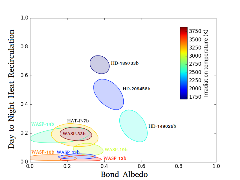
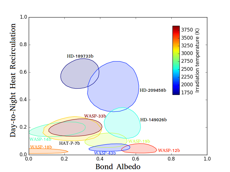
We show two versions of the albedo-efficiency plot in Figure 12 , including one with all published thermal secondary eclipse and phase curve data and another which only considers 3.6 and 4.5 µm Spitzer data in order to ensure a more uniform analysis. The only planet that moved significantly was WASP-12b.

This figure shows that WASP-33b has a Bond albedo and recirculation efficiency that appear largely similar to those of other hot Jupiters despite its high irradiation level. HD 149026b, however, appears to have an unusually high albedo in our toy model. Its best-fit albedo is higher than that of all other planets with thermal phase curves, and it is also higher than any of the optical geometric albedos measured by Kepler as shown by Figure 7 of Schwartz & Cowan (2015). This might reasonably be explained by the presence of a reflective cloud layer in this planet’s upper atmosphere; the presence of such a cloud layer could be confirmed with future transmission spectroscopy.

Parmentier et al. (2016) calculated the effective cloud coverage for a range of equilibrium temperatures, three cloud top pressures, and a number of cloud compositions. Although they focused on investigating the role of clouds at optical wavelengths rather than in the Spitzer bands, we can nonetheless utilize their results to explore the potential cloud species that might be present in HD 149026b’s atmosphere. They report evidence for the presence of silicate clouds for $T_{eq}>1600K$, presence of MnS clouds for $T_{eq}<1600K$, and absence of silicate clouds for $T_{eq}<1600K$. HD 149026b has a zero-albedo equilibrium temperature of 1700 K, very close to the 1600 K dividing line. If there are silicate clouds, their Figure 13 shows that the dayside effective cloud coverage is expected to be 30-80%, depending on the cloud top pressure, while the nightside coverage is 50-100%. If there are MnS clouds but no silicate clouds, the dayside cloud coverage would be 0-20%, while the nightside cloud coverage would be 20-100%.

Mahapatra et al. (2017) used a kinetic, non-equilibrium cloud formation model to study cloud structures and compositions. For HD 149026b, they found that clouds are likely composed of many different species, with TiO₂ dominant at the cloud top ($10^{2.5}$ bar) while species such as Fe, SiO, and MgSiO₃ are common deeper down.

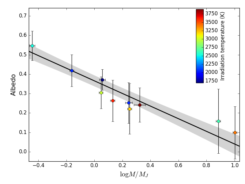
One of the most interesting aspects of Figure 12 is that it shows no obvious correlations between irradiation temperature, albedo, and efficiency. In fact, it appears that planets with very different irradiation temperatures can have similar albedos and recirculation efficiencies. We plotted mass versus efficiency, irradiation temperature versus albedo, and irradiation temperature versus efficiency, finding that the two least massive planets in our sample–HD 149026b and HD 209458b–are outliers in both albedo and efficiency. In Wong et al. (2015b) we previously suggested a possible correlation between mass and albedo, but after additional data was collected, we concluded in Wong et al. (2016) that a simple mass-albedo correlation was no longer tenable. However, we see a strong correlation when we plot these two parameters in Figure 13. The linear model has a lower BIC than the constant-albedo model ($\Delta BIC=-12.5$), indicating a strong preference for the linear model. In addition, the error bars on the albedo seem overestimated, possibly due to the large systematic error we deliberately introduce (in accordance with Cowan & Agol 2011) in converting from brightness temperature to physical temperature. After subtracting the best fit linear model, we find $\chi^{2}=1.86$ for the residuals; with 8 degrees of freedom, there is only a 1.5% probability of obtaining a $\chi^{2}$ this low. If the errors were correctly estimated, $\Delta BIC$ would be even more negative, preferring the linear model even more strongly. Our best fit line has slope $m=-0.326\pm 0.047$ and intercept $b=0.366\pm 0.016$. Coincidentally, 0.366 is very close to the Bond albedo of Jupiter itself.

The physical explanation for the decrease in albedo with mass is unclear. One possibility is that increased surface gravity makes it harder for cloud particles to be kept aloft, as shown in Equation 10 of Heng & Demory (2013). The increased cloudiness at low surface gravity has been observed on brown dwarfs (Faherty et al., 2016). The main difficulty with this explanation is that we have also plotted the relation between surface gravity and albedo, and although an anticorrelation is seen, it is much less statistically significant than the mass-albedo correlation ($\Delta BIC=-2.4$, compared to $\Delta BIC=-12.5$).

4.4.1 Phase curve offsets

The toy model discussed above derives recirculation efficiency from the observed nightside flux. However, the nightside flux can only be measured by reference to the secondary eclipse, which is hours or days away. This makes the measurement particularly sensitive to instrumental noise sources on long timescales, including the long-term pointing drift present in many phase curve observations. As an example, the Spitzer phase curves for WASP-43b imply a negative nightside flux, which is unphysical (Keating & Cowan, 2017).

In this section we explore correlations between phase offset and other planetary parameters. In GCMs, both the size of the phase offset and the relative temperature gradient between the day and night sides increase with increasing depth (pressure) in the atmosphere (e.g., Showman et al. 2009). We therefore consider whether or not the measured phase offset might be useful as a proxy for recirculation efficiency. We plotted recirculation efficiency against phase offset and found that although planets with very large phase offsets have somewhat high efficiencies and planets with very small phase offsets have somewhat low efficiencies, the correlation is by no means exact. We conclude that either phase offset is an imperfect proxy for recirculation efficiency in practice, or the recirculation efficiency calculated using our simple toy model is simply not accurate enough for the correlation to be obvious.

Figure 14.— Phase offset vs. irradiation temperature for all hot Jupiters on circular orbits with thermal phase curves. Blue represents 3.6 µm while red represents 4.5 µm. The light blue point is the 3.6 µm observation for HD 149026b, which we discuss in §4.1. The black lines represent the best-fit bilinear model, while the gray region indicates the 1$\sigma$ confidence interval.

Figure 15.— Phase offset vs. irradiation temperature for GCM-modeled planets. The green line is the best fit linear model to the GCM data, while the black lines represent the best fit bilinear model to the observations. The black lines are identical to the ones in Figure 14.

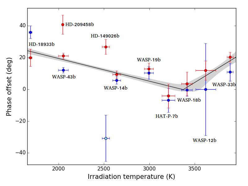
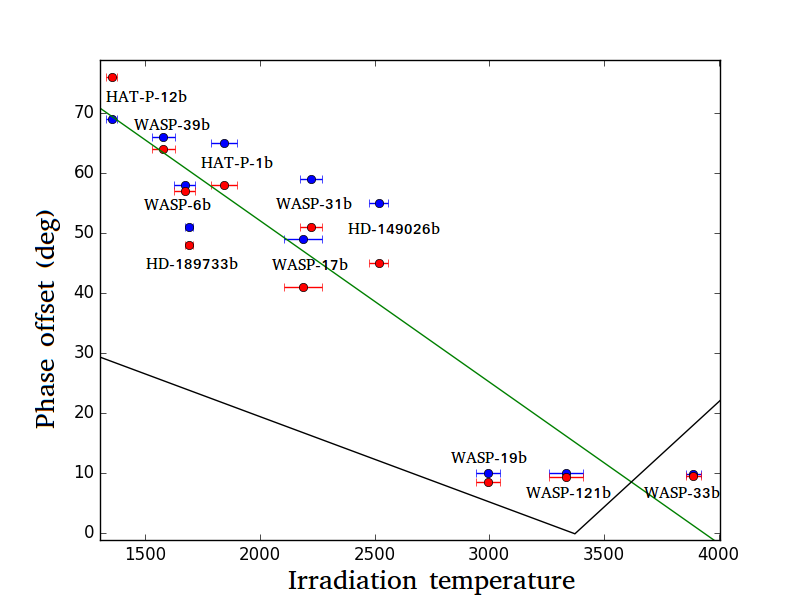
Figure 14 shows a strong correlation between a planet’s irradiation temperature $T_{0}=T_{\rm eff}/\sqrt{a_{*}}$ and its phase offset. There is a clear downward trend until $3400K$, after which the trend reverses direction. We tested the significance of the trend by fitting the data with five models: a constant phase model, a linear model, a bilinear model, a bilinear model with the slope of the second line segment fixed to 0, and a bilinear model with both the slope and intercept of the second line segment fixed to 0. We obtain a BIC of 185, 168, 136, 145, and 186 respectively. Thus, the reversal at $3400K$, despite being based on only three data points, is significant from a purely statistical perspective. The fit results for the first line segment are $b_{1}=47.7\degree\pm 4.7\degree$, $m_{1}=-0.014\pm 0.002$ deg/K; for the crossover point, $T_{c}=3410\pm 110$; and for the second line segment, $m_{2}=0.039_{-0.011}^{+0.017}$ deg/K.

Despite the statistical significance, the rise is still based only three planets, and may not be real. The test assumes Gaussian errors, while the actual errors are in reality both asymetric and non-Gaussian. Even more importantly, Spitzer light curves are notorious for having bizarre and unexplained instrumental systematics which can affect the fitted parameters in ways that are subtle and difficult to diagnose. In this paper alone, we have seen this for HD 149026b in the 3.6 µm band, and WASP-12b for two different observations in the 3.6 µm band. Other examples of problematic behavior include Stevenson et al. (2017), where two separate visits in the same band resulted in very different nightside fluxes. A sprinkling of unmodelled systematics, plus a smattering of bad luck, could be sufficient to destroy the final rise in temperature.

On the other hand, there are physical reasons to be less skeptical. First, although the reversal at $3400K$ has never been predicted or previously noted, the initial drop is unsurprising–phase offsets are expected to decrease with increasing temperature because the radiative timescale drops steeply with temperature (Perez-Becker & Showman, 2013; Komacek & Showman, 2016). Second, it is also clear that some kind of break must occur at $3400K$–if the downward trend continued, the phase offset would become westward at higher temperatures, which is physically implausible.

The only significant outlier in this trend is the 3.6 µm observation for HD 149026b, which we discuss in §4.1. Additionally, as discussed in §4.4, Cowan et al. (2012) presented two contradictory sets of results for WASP-12b’s phase curve, based on two distinct analysis methods. Had we used the other version, the 4.5 µm phase curve offset would have been nearly identical, but the 3.6 µm phase curve offset would be at a physically implausible 53$\arcdeg$–another clear outlier. The fact that both potential outliers in this plot are based on problematic data sets gives confidence to the reality of the trend. The trend is even more striking when one considers that it is between two relatively reliably measured quantities. The irradiation temperature is dependent only on the stellar effective temperature and $a/R_{*}$, both of which are easily measured. The phase offset is harder to measure (e.g., §4.4), but unlike albedos and efficiencies, it is a purely empirical quantity.

To understand this trend, we took previously published SPARC GCM simulations (Kataria et al., 2016) and plotted phase offset against irradiation temperature in Figure 15. The sample of planets in these GCMs is different from those presented in the observations. All models are at solar metallicity and have no TiO, in order to ensure a more uniform comparison. As expected, the predicted phase offsets from these models decrease with increasing irradiation temperature until approximately 3000 K. The offsets decrease at a rate of $-0.017$ deg/K. However, instead of rising towards the highest temperatures they instead plateau around a minimum phase offset of approximately 10$\arcdeg$. It is also worth noting that in these models the 3.6 µm bandpass has a larger phase shift (by an average of 4.1$\arcdeg$) for all but the coolest planet, indicating that this wavelength probes deeper into the atmosphere. In our observations, the 4.5 µm phase curves have larger phase shifts (and thus deeper photospheres) than the 3.6 µm phase curves for every planet except the coldest, the average difference being 6.2 degrees. The universality of this trend among our relatively diverse sample of hot Jupiters is suggestive, and should help guide future modeling efforts in this area.

There are a combination of factors that may or may not explain the discrepancy between observations and GCMs. For example, the addition of high altitude clouds to the GCMs could help by decreasing the dayside photospheric pressure, which would systematically reduce the size of the predicted phase offsets and provide a better match to the observational data. Such clouds appear to provide a good match to the optical phase curve offsets measured for the hot Jupiters located in the Kepler field (Parmentier et al., 2016; Demory et al., 2013; Shporer & Hu, 2015; Angerhausen et al., 2015) and have also been postulated to explain other infrared phase-curve observations (e.g. Kataria et al., 2015; Stevenson et al., 2017). However, Roman & Rauscher (2017) complicate this explanation by showing that clouds do not always lead to lower phase offsets. They find that in the case of Kepler-7b, inhomogenous clouds distributed along the western terminator result in a higher phase offset, while global clouds result in a marginally lower offset, compared to the clear atmosphere case. A super-solar metallicity atmosphere could also provide a similar effect; enhanced metallicity results in enhanced opacities, such that the photosphere is higher in the atmosphere where the day-night contrast is larger and the phase offset is smaller (e.g., Kataria et al. 2015). At high temperatures, the presence of dayside temperature inversions produced by gas-phase TiO/VO might also affect the predicted phase offsets, as this will change the opacity of the atmosphere and hence what altitudes are probed (e.g., Showman et al. 2009).

MHD effects such as Lorentz drag and Ohmic dissipation are also likely to be important (e.g., Perna et al. 2010; Batygin & Stevenson 2010; Menou 2012; Rauscher & Menou 2012; Ginzburg & Sari 2016). Because Lorentz drag and Ohmic dissipation are two facets of the same underlying processes, we can turn to the literature on Ohmic dissipation and radius inflation in hot Jupiters to determine the regime in which these effects become important. For hot Jupiters with an appreciable magnetic field, the effect of this magnetic field on the atmospheric circulation will depend on the ionization fraction of the planet’s upper atmosphere. Previous models have concluded that alkali metals such as Na and K will provide the dominant source of ions in these atmospheres (e.g., Batygin & Stevenson 2010). As the ionization fraction increases the strength of the Lorentz drag and also the amount of radius inflation due to Ohmic dissipation increase as well, resulting in a peak radius inflation at equilibrium temperatures of around 1500 K. At higher temperatures, the atmospheric circulation is effectively suppressed by the magnetic drag and less energy is deposited in the planet’s interior. Thorngren & Fortney (2017) find compelling evidence for a peak in the radius inflation of hot Jupiters around 1500 K and a decline thereafter, in good agreement with these models. With this picture in mind, the addition of Lorentz drag around 1500 K is likely the explanation for why the observed phase offsets at higher temperatures decrease to values consistent with zero, while the GCMs predict a minimum phase offset around 10$\arcdeg$. However, this simple picture appears to conflict with the observed increase in phase offset for the most highly irradiated planets, as the amount of Lorentz drag should remain constant over this highly irradiated regime. Although there has been some recent work on atmospheric circulation in the MHD-dominated regime (e.g., Rogers 2017), it is not yet clear whether more careful modeling can reproduce the observed trend in phase offsets at these temperatures.

As a last point, we consider possible explanations for the relative offsets observed between the two Spitzer bands. As noted earlier, the measured 4.5 µm offset is consistent larger than the measured 3.6 µm offset for every planet except for HD 189733b, but the opposite is consistently true in the model predictions for these planets. Atmospheric chemistry would seem to be the obvious explanation: CH₄ is a major absorber within the 3.6 µm bandpass, while CO is a strong absorber within the 4.5 µm bandpass, so the relative abundances of these two molecules could easily shift the relative photospheric pressures in these two bands. Increasing the amount of CH₄ via vertical mixing or other disequilibrium chemistry processes would increase the opacity and decrease the photospheric pressure in the 3.6 µm band, resulting in a larger day-night contrast and smaller phase offset. Similarly, decreasing the amount of CO in the atmosphere would decrease the opacity in the 4.5 µm band, shifting the photosphere to higher pressures with a smaller day-night temperature contrast and a larger phase offset. Still, an enhanced methane abundance would require a drastic departure from equilibrium chemistry, as CO is expected to be the major carbon-bearing molecule at temperatures relevant to hot Jupiters. Madhusudhan et al. (2014), for example, show that the delineation between CO and CH₄ dominance at 1500 K is at 10 bars, rising to 100 bars at 2000 K. For hot planets the abundance of CH₄ at photospheric pressures (approx. 100 mbar) should be tiny. Even for HD 189733b, the coldest planet in Figure 14, the CH₄ abundance is nearly 3 orders of magnitude below the CO abundance for any reasonable photospheric pressure, as shown in Figure 3 of Madhusudhan et al. (2014).

5. Conclusions

In this paper we present new phase curve observations for WASP-33b and HD 149026b at 3.6 µm and 4.5 µm. Our measured parameters are in good agreement with previously published transit and secondary eclipse observations of these two planets, and we use our new phase curve observations to investigate the atmospheric circulation patterns of these two planets. We use a simple toy model to estimate the brightness temperatures, albedo, and recirculation efficiency of both planets under the assumption that they emit as blackbodies and find that WASP-33b appears generally similar to other hot Jupiters despite its unusually high irradiation level. On the other hand, HD 149026b has a typical recirculation efficiency but an albedo of 0.6–the highest ever measured. This albedo strongly suggests the presence of clouds, which could easily be confirmed with HST transmission spectroscopy. Intriguingly, we find strong evidence for a correlation between the masses of planets with published thermal phase curves and their inferred albedos; this may be indicative of the role that surface gravity plays in the settling of cloud particles.

We also compared our measured phase curves for these two planets to predictions from GCMs. For HD 149026b, we considered models with $1\times$ and $30\times$ solar metallicity, both of which provided an unusually poor match to the observed phase curve shapes. Based on this planet’s high inferred albedo and enhanced bulk metallicity, it seems likely that even higher metallicity GCMs incorporating clouds could provide a better match to these data. For WASP-33b, we considered models with and without TiO; although there were still some discrepancies, these models were overall a much better fit than in the case of HD 149026b. We note that MHD effects likely dominate the atmospheric circulation for highly irradiated planets like WASP-33b, and present an obvious avenue for future investigations.

Lastly, we placed these two planets in context by comparing their observed phase offsets in each band to those of other planets. We find a strong correlation between measured phase offset and irradiation temperature, where the observed offset decreases with increasing irradiation temperature to a minimum around 3400 K, and then rises again for the most highly irradiated planets. Although this decreasing trend with increasing irradiation is predicted by GCM simulations of these planets, in practice the size of the observed phase offsets for the coolest planets appear to be lower than predicted by the GCMs. We propose that this can be explained by the presence of high altitude cloud layers in these atmospheres, which decrease the photospheric pressure probed in these two bands. At higher temperatures, we find that the observed phase offsets decrease to zero for irradiation temperatures near 3400 K, while the GCMs predict a minimum phase offset of 10$\arcdeg$ for planets in this temperature regime. We propose that this discrepancy can be resolved by the inclusion of MHD effects such as Lorentz drag, which would serve to further reduce the speed of atmospheric winds and decrease the size of the observed phase offset. We note that the trend of increasing phase offset with increasing temperature for the most highly irradiated planets is not well-matched by this simple picture, but perhaps could be explained with more sophisticated circulation models incorporating the full range of MHD effects. Finally, we propose that the relative phase offsets at 3.6 and 4.5 µm, which are consistently the opposite of those predicted in the GCMs, might be explained by a change in the assumed atmospheric compositions and/or chemistries of these planets.

6. Acknowledgments

This work is based on observations made with the Spitzer Space Telescope, which is operated by the Jet Propulsion Laboratory, California Institute of Technology under a contract with NASA. Support for this work was provided by NASA through an award issued by JPL/Caltech. H.A.K. acknowledges support from the Sloan Foundation.

References

- Adcroft et al. (2004) Adcroft, A., Campin, J.-M., Hill, C., & Marshall, J. 2004, Monthly Weather Review, 132, 2845
- Angerhausen et al. (2015) Angerhausen, D., DeLarme, E., & Morse, J. A. 2015, PASP, 127, 1113
- Astropy Collaboration et al. (2013) Astropy Collaboration, Robitaille, T. P., Tollerud, E. J., et al. 2013, A&A, 558, A33
- Batygin & Stevenson (2010) Batygin, K., & Stevenson, D. J. 2010, ApJ, 714, L238
- Benneke et al. (2017) Benneke, B., Werner, M., Petigura, E., et al. 2017, ApJ, 834, 187
- Bradley et al. (2016) Bradley, L., Sipocz, B., Robitaille, T., et al. 2016, astropy/photutils: v0.3
- Burrows et al. (2008) Burrows, A., Budaj, J., & Hubeny, I. 2008, ApJ, 678, 1436
- Burrows et al. (2010) Burrows, A., Rauscher, E., Spiegel, D. S., & Menou, K. 2010, ApJ, 719, 341
- Carter et al. (2009) Carter, J. A., Winn, J. N., Gilliland, R., & Holman, M. J. 2009, ApJ, 696, 241
- Charbonneau et al. (2005) Charbonneau, D., Allen, L. E., Megeath, S. T., et al. 2005, ApJ, 626, 523
- Charbonneau et al. (2006) Charbonneau, D., Winn, J. N., Latham, D. W., et al. 2006, ApJ, 636, 445
- Collier Cameron et al. (2010) Collier Cameron, A., Guenther, E., Smalley, B., et al. 2010, MNRAS, 407, 507
- Cooper & Showman (2005) Cooper, C. S., & Showman, A. P. 2005, ApJ, 629, L45
- Cooper & Showman (2006) —. 2006, ApJ, 649, 1048
- Cowan & Agol (2008) Cowan, N. B., & Agol, E. 2008, ApJ, 678, L129
- Cowan & Agol (2011) Cowan, N. B., & Agol, E. 2011, The Astrophysical Journal, 729, 54
- Cowan et al. (2012) Cowan, N. B., Machalek, P., Croll, B., et al. 2012, ApJ, 747, 82
- de Mooij et al. (2013) de Mooij, E. J. W., Brogi, M., de Kok, R. J., et al. 2013, A&A, 550, A54
- Deming et al. (2012) Deming, D., Fraine, J. D., Sada, P. V., et al. 2012, ApJ, 754, 106
- Deming et al. (2015a) Deming, D., Knutson, H., Kammer, J., et al. 2015a, ApJ, 805, 132
- Deming et al. (2015b) —. 2015b, ApJ, 805, 132
- Demory et al. (2013) Demory, B.-O., de Wit, J., Lewis, N., et al. 2013, ApJ, 776, L25
- Dodson-Robinson & Bodenheimer (2009) Dodson-Robinson, S. E., & Bodenheimer, P. 2009, ApJ, 695, L159
- Faherty et al. (2016) Faherty, J. K., Riedel, A. R., Cruz, K. L., et al. 2016, ApJS, 225, 10
- Fazio et al. (2004) Fazio, G. G., Hora, J. L., Allen, L. E., et al. 2004, ApJS, 154, 10
- Foreman-Mackey et al. (2017) Foreman-Mackey, D., Agol, E., Angus, R., & Ambikasaran, S. 2017, ArXiv
- Foreman-Mackey et al. (2013) Foreman-Mackey, D., Hogg, D. W., Lang, D., & Goodman, J. 2013, PASP, 125, 306
- Fortney et al. (2006) Fortney, J. J., Cooper, C. S., Showman, A. P., Marley, M. S., & Freedman, R. S. 2006, ApJ, 652, 746
- Fortney et al. (2008) Fortney, J. J., Lodders, K., Marley, M. S., & Freedman, R. S. 2008, ApJ, 678, 1419
- Ginzburg & Sari (2016) Ginzburg, S., & Sari, R. 2016, ApJ, 819, 116
- Grillmair et al. (2012) Grillmair, C. J., Carey, S. J., Stauffer, J. R., et al. 2012, in Proc. SPIE, Vol. 8448, Observatory Operations: Strategies, Processes, and Systems IV, 84481I
- Haynes et al. (2015) Haynes, K., Mandell, A. M., Madhusudhan, N., Deming, D., & Knutson, H. 2015, ApJ, 806, 146
- Heng & Demory (2013) Heng, K., & Demory, B.-O. 2013, ApJ, 777, 100
- Heng & Showman (2015) Heng, K., & Showman, A. P. 2015, Annual Review of Earth and Planetary Sciences, 43, 509
- Hubeny et al. (2003) Hubeny, I., Burrows, A., & Sudarsky, D. 2003, ApJ, 594, 1011
- Husser et al. (2013) Husser, T.-O., Wende-von Berg, S., Dreizler, S., et al. 2013, A&A, 553, A6
- Ingalls et al. (2012) Ingalls, J. G., Krick, J. E., Carey, S. J., et al. 2012, in Proc. SPIE, Vol. 8442, Space Telescopes and Instrumentation 2012: Optical, Infrared, and Millimeter Wave, 84421Y
- Ingalls et al. (2016) Ingalls, J. G., Krick, J. E., Carey, S. J., et al. 2016, AJ, 152, 44
- Johnson et al. (2015) Johnson, M. C., Cochran, W. D., Collier Cameron, A., & Bayliss, D. 2015, ApJ, 810, L23
- Kammer et al. (2015) Kammer, J. A., Knutson, H. A., Line, M. R., et al. 2015, ApJ, 810, 118
- Kass & Raftery (1995) Kass, R. E., & Raftery, A. E. 1995, Journal of the American Statistical Association, 90, 773
- Kataria et al. (2015) Kataria, T., Showman, A. P., Fortney, J. J., et al. 2015, ApJ, 801, 86
- Kataria et al. (2016) Kataria, T., Sing, D. K., Lewis, N. K., et al. 2016, ApJ, 821, 9
- Keating & Cowan (2017) Keating, D., & Cowan, N. B. 2017, ArXiv e-prints, 1709.03502
- Knutson et al. (2009) Knutson, H. A., Charbonneau, D., Cowan, N. B., et al. 2009, ApJ, 703, 769
- Knutson et al. (2012) Knutson, H. A., Lewis, N., Fortney, J. J., et al. 2012, ApJ, 754, 22
- Komacek & Showman (2016) Komacek, T. D., & Showman, A. P. 2016, ApJ, 821, 16
- Kovács et al. (2013) Kovács, G., Kovács, T., Hartman, J. D., et al. 2013, A&A, 553, A44
- Kreidberg (2015) Kreidberg, L. 2015, PASP, 127, 1161
- Lehmann et al. (2015) Lehmann, H., Guenther, E., Sebastian, D., et al. 2015, A&A, 578, L4
- Lewis et al. (2014) Lewis, N. K., Showman, A. P., Fortney, J. J., Knutson, H. A., & Marley, M. S. 2014, ApJ, 795, 150
- Lewis et al. (2010) Lewis, N. K., Showman, A. P., Fortney, J. J., et al. 2010, ApJ, 720, 344
- Lewis et al. (2013) Lewis, N. K., Knutson, H. A., Showman, A. P., et al. 2013, ApJ, 766, 95
- Luger et al. (2016) Luger, R., Agol, E., Kruse, E., et al. 2016, AJ, 152, 100
- Madhusudhan et al. (2014) Madhusudhan, N., Knutson, H., Fortney, J. J., & Barman, T. 2014, Protostars and Planets VI, 739
- Mahapatra et al. (2017) Mahapatra, G., Helling, C., & Miguel, Y. 2017, MNRAS, 472, 447
- Mancini et al. (2016) Mancini, L., Kemmer, J., Southworth, J., et al. 2016, MNRAS, 459, 1393
- Marley & McKay (1999) Marley, M. S., & McKay, C. P. 1999, Icarus, 138, 268
- Menou (2012) Menou, K. 2012, ApJ, 745, 138
- Morley et al. (2017) Morley, C. V., Knutson, H., Line, M., et al. 2017, AJ, 153, 86
- Moses et al. (2013) Moses, J. I., Line, M. R., Visscher, C., et al. 2013, ApJ, 777, 34
- Nugroho et al. (2017) Nugroho, S. K., Kawahara, H., Masuda, K., et al. 2017, ArXiv e-prints, 1710.05276
- Nutzman et al. (2009) Nutzman, P., Charbonneau, D., Winn, J. N., et al. 2009, ApJ, 692, 229
- Parmentier et al. (2016) Parmentier, V., Fortney, J. J., Showman, A. P., Morley, C., & Marley, M. S. 2016, ApJ, 828, 22
- Perez-Becker & Showman (2013) Perez-Becker, D., & Showman, A. P. 2013, ApJ, 776, 134
- Perna et al. (2010) Perna, R., Menou, K., & Rauscher, E. 2010, ApJ, 719, 1421
- Rauscher & Menou (2012) Rauscher, E., & Menou, K. 2012, ApJ, 750, 96
- Rogers (2017) Rogers, T. M. 2017, Nature Astronomy, 1, 0131
- Roman & Rauscher (2017) Roman, M., & Rauscher, E. 2017, ApJ, 850, 17
- Sato et al. (2005) Sato, B., Fischer, D. A., Henry, G. W., et al. 2005, The Astrophysical Journal, 633, 465
- Schwartz & Cowan (2015) Schwartz, J. C., & Cowan, N. B. 2015, MNRAS, 449, 4192
- Schwartz et al. (2017) Schwartz, J. C., Kashner, Z., Jovmir, D., & Cowan, N. B. 2017, ArXiv e-prints, 1707.05790
- Seager & Deming (2010) Seager, S., & Deming, D. 2010, ARA&A, 48, 631
- Showman et al. (2009) Showman, A. P., Fortney, J. J., Lian, Y., et al. 2009, ApJ, 699, 564
- Showman & Guillot (2002) Showman, A. P., & Guillot, T. 2002, A&A, 385, 166
- Shporer & Hu (2015) Shporer, A., & Hu, R. 2015, AJ, 150, 112
- Sing (2010) Sing, D. 2010, Limb Darkening, http://www.astro.ex.ac.uk/people/sing/David_Sing/Limb_Darkening.html, accessed: 2017-03-29
- Sing et al. (2016) Sing, D. K., Fortney, J. J., Nikolov, N., et al. 2016, Nature, 529, 59
- Smith et al. (2011) Smith, A. M. S., Anderson, D. R., Skillen, I., Collier Cameron, A., & Smalley, B. 2011, MNRAS, 416, 2096
- Stevenson (2016) Stevenson, K. B. 2016, ApJ, 817, L16
- Stevenson et al. (2012) Stevenson, K. B., Harrington, J., Fortney, J. J., et al. 2012, ApJ, 754, 136
- Stevenson et al. (2017) Stevenson, K. B., Line, M. R., Bean, J. L., et al. 2017, AJ, 153, 68
- Thorngren & Fortney (2017) Thorngren, D. P., & Fortney, J. J. 2017, ArXiv e-prints, 1709.04539
- Torres et al. (2008) Torres, G., Winn, J. N., & Holman, M. J. 2008, ApJ, 677, 1324
- Turner et al. (2016) Turner, J. D., Pearson, K. A., Biddle, L. I., et al. 2016, MNRAS, 459, 789
- von Essen et al. (2015) von Essen, C., Mallonn, M., Albrecht, S., et al. 2015, A&A, 584, A75
- von Essen et al. (2014) von Essen, C., Czesla, S., Wolter, U., et al. 2014, A&A, 561, A48
- Wakeford et al. (2017) Wakeford, H. R., Sing, D. K., Kataria, T., et al. 2017, Science, 356, 628
- Winn et al. (2008) Winn, J. N., Henry, G. W., Torres, G., & Holman, M. J. 2008, ApJ, 675, 1531
- Wong et al. (2015a) Wong, I., Knutson, H. A., Lewis, N. K., et al. 2015a, ApJ, 811, 122
- Wong et al. (2015b) —. 2015b, ApJ, 811, 122
- Wong et al. (2016) Wong, I., Knutson, H. A., Kataria, T., et al. 2016, ApJ, 823, 122
- Zellem et al. (2014) Zellem, R., Griffith, C. A., Lewis, N. K., Swain, M. R., & Knutson, H. A. 2014, in AAS/Division for Planetary Sciences Meeting Abstracts, Vol. 46, AAS/Division for Planetary Sciences Meeting Abstracts, 104.04