Asymptotically Optimal Resource Block Allocation With Limited Feedback

Abstract

Consider a channel allocation problem over a frequency-selective channel. There are $K$ channels (frequency bands) and $N$ users such that $K=bN$ for some positive integer $b$. We want to allocate $b$ channels (or resource blocks) to each user. Due to the nature of the frequency-selective channel, each user considers some channels to be better than others. The optimal solution to this resource allocation problem can be computed using the Hungarian algorithm. However, this requires knowledge of the numerical value of all the channel gains, which makes this approach impractical for large networks. We suggest a suboptimal approach, that only requires knowing what the $M$-best channels of each user are. We find the minimal value of $M$ such that there exists an allocation where all the $b$ channels each user gets are among his $M$-best. This leads to feedback of significantly less than one bit per user per channel. For a large class of fading distributions, including Rayleigh, Rician, m-Nakagami and others, this suboptimal approach leads to both an asymptotically (in $K$) optimal sum-rate and an asymptotically optimal minimal rate. Our non-opportunistic approach achieves (asymptotically) full multiuser diversity as well as optimal fairness, by contrast to all other limited feedback algorithms.

I Introduction

The problem of multiple users accessing a common medium is a central issue in every communication network [2, 3, 4]. The most common access schemes in practice are orthogonal transmission techniques such as TDMA, FDMA , CDMA and OFDMA [5, 6]. Modern communication networks allocate each user a number of resource blocks, each consisting of several OFDMA subcarriers that need not be adjacent [7].

When using a frequency division technique in a frequency-selective channel, not all channels have the same quality. Furthermore, since different users have different positions, the channel gains of users in a given frequency band are independent. This introduces a resource allocation problem between users and frequency bands (channels). Theoretically, if the exact knowledge of all these channel gains were available, an optimal solution for this resource allocation could be computed. The performance gain that can be achieved by solving this problem over a frequency allocation that ignores the channel gains is known as multiuser diversity [8].

In FDD systems, the base station (BS) can only have knowledge of the channel gains of each user if all users transmit this information directly. In TDD systems, the BS can estimate the channel gain of a given user from the reciprocity of the channel. However, the BS must estimate the channel gains in all frequencies, not just the currently used ones, so a wideband transmission is required from each user. These transmissions need to be coordinated between users so that they will not collide. Moreover, although the channels are indeed reciprocal, the RF circuits are not, which calls for a calibration process [9].

As networks grow and bandwidth expands, the number of channels increases significantly. This is typical of OFDMA systems that tend to have a large number of subcarriers. For example, in LTE [7] there are from 128 to 2048 subcarriers in the downlink for each user. This implies that reporting the channel state information (CSI) to the BS inflicts a large communication overhead that makes such a scheme infeasible.

This paper deals with a channel allocation task with $K$ channels where $N$ users simultaneously demand $b$ channels for each. This occurs when users are backlogged; i.e., always have packets to transmit. This represents a non-opportunistic approach where the BS waits for a queue of $N$ users to form and only then computes a good allocation for all the users in the queue. When users leave the network and others replace them, the allocation is updated accordingly.

We propose a novel limited feedback scheme that significantly reduces feedback overhead compared to state of the art techniques [10, 11, 12, 13, 14]. The proposed technique provides a provably both asymptotically optimal sum-rate and max-min fairness (which none of the current methods provide). The proof applies to a wide range of fading distributions that includes Rayleigh, Rician and m-Nakagami. Our technique uses ~0.85 bits per user per channel for $K=N=20$, and ~0.52 bits per user per channel for $K=512$ and $N=128$.

In our approach, users only need to feed back the indices of their $M$-best channels, and not their numerical values. If $M$ is large enough, there is a high probability of an allocation of users to channels where each user gets $b$ channels, all of which are from his $M$-best channels. We prove that for $M\geq\left(b+1\right)\left(1+\varepsilon\right)\ln K$, for $\varepsilon>0$, this probability approaches one as $K\rightarrow\infty$. While our approach is asymptotic, the probability that such a perfect matching allocation exists exceeds 99% for $K=20$ channels and $N=20$ users.

Figure 1 presents a toy example of our system with $N=K=4$. Each user transmits the indices of his $M$ best channels to the BS. The BS constructs the associated bipartite graph, computes a perfect matching in this graph and transmits back the allocated channel to each user.

The existence of a perfect matching allocation relies on the theory of random bipartite graphs. We define a novel random bipartite graph where each user is represented by $b$ vertices (“agents”) in the graph, all of which are connected to the $M$-best channels of this user on the other side of the graph. We prove that this bipartite graph has a perfect matching, with high probability. Due to its dependent edges, our random bipartite graph is not an Erdős–Rényi graph. Consequently, proving the existence of a perfect matching requires revisiting the original proof. Our proof is in the spirit of the original result by Erdős and Rényi for random bipartite graphs [15]. A generalization of our results to the case of unequal numbers of channels between users can be achieved using the same techniques. It is omitted due to the complicated formalism. However, we present detailed simulations of the CDF of the rates (not just the means) that indicate that our results are also valid for an unequal number of channels between users.

Throughout this paper, we use the term “channel”. This may represent several united subcarriers if the coherence bandwidth is large and they are highly correlated (e.g., a resource block). In other words, a “channel” is a designed unit that should optimally be the smallest independent resource block in terms of the statistics of the corresponding channel gain.

I-A Related Work

There is extensive literature on OFDMA resource allocation (see the surveys in [16, 17] and the references therein). These allocations deal with the subcarrier assignment and the power allocation over these subcarriers. The state of the art algorithms achieve a close to optimal sum-rate with reduced computational complexity compared to the optimal solution. In many studies, it has been shown that an equal power allocation between the subcarriers of each user achieves very close to optimal performance [18, 19, 20, 21, 22, 23]. Hence, the problem of subcarrier allocation appears to be much more significant than that of power allocation. However, all these approaches assume that users estimate their CSI perfectly and feed all of it back to the BS. While this assumption may be reasonable for small networks, it is highly infeasible for large networks with a large number of subcarriers, such as LTE [7].

In order to overcome the need for the whole CSI to exploit the selectivity of the channel, many works have suggested suboptimal schemes with limited feedback. For an excellent overview of limited feedback systems, see [24]. The state of the art algorithms consider an opportunistic scheduling approach, where each available channel is assigned to a user with a high instantaneous channel gain [10, 11, 25, 12].

In [10, 11, 12] each user transmits one bit per channel to indicate if the corresponding channel gain exceeds a threshold, while in [25] each user transmits the highest-rate modulation scheme he can support out of a discrete set of schemes (which requires more than one bit per channel). In [26, 27], channels are grouped together into clusters and only the information about the quality of each cluster is transmitted by the user. This grouping approach limits the amount of multiuser diversity that can be achieved, so that the reduced feedback has a performance cost. This cost is avoided if the grouped subcarriers are highly correlated, but in this case the multiuser diversity is smaller. We argue that for highly correlated channels, using grouping cannot be considered a real feedback reduction, since assigning two bits to two highly correlated subcarriers is a waste of feedback to begin with. In this work we use the term “channel” to refer to the smallest group of subcarriers for which the "channels" are independent, which can be considered a kind of grouping.

In [13], the grouping and thresholding approaches were combined to achieve a feedback of less than one bit per user per channel, which leads to a compromise of suboptimal performance (even asymptotically). In [14], the $M$-best channels approach was used for opportunistic scheduling. Users are arranged in a queue, and each of them transmits the indices of his $M$-best channels to the BS. The BS sequentially assigns each user the best channel from these $M$ channels if it is available, and a random channel if none of them are. The thresholding approach requires the BS or the users to know the fading distribution to compute the optimal threshold. The $M$-best channels approach does not require any such knowledge, which makes it more robust.

All these approaches are opportunistic in nature and as such suffer from an inherent unfairness. Some of the methods have suggested obtaining some degree of fairness by designing the scheduler [27, 11, 12, 10], at the cost of a reduced sum-rate. In order to get a comparable sum-rate with a proportional fairness scheduler, each user needs to wait until he is chosen as the “opportunistic user”. Therefore, fairness can only be maintained by introducing very large delays for users, which is far from being desirable or practical.

The rationale behind the opportunistic approach is to exploit the multiuser diversity. By contrast, here we argue that this widespread approach is too conservative and that achieving multiuser diversity should not come at the expense of fairness. We argue that fairness is undermined because all these approaches schedule a user for each channel separately. Somewhat surprisingly, when analyzing all the channels together, each user is very likely to be “an opportunistic choice” for some available channel. This calls for a more sophisticated mathematical analysis of the random matchings between users and channels as we employ in this paper, in contrast to the simplistic arguments dealing with either one user or one channel at a time.

In contrast to [12, 13, 14, 11], our work is not limited to Rayleigh-fading channels, but applies to a much broader class of exponentially-dominated tail distributions. Besides Rayleigh fading, this class includes Rician, m-Nakagami and others.

In [28, 29, 30], a distributed channel allocation for Ad-Hoc networks was introduced, based on a carrier-sensing multiple access (CSMA) scheme and a thresholding approach for the channel gains. Although considering a different scenario, the analysis in [28, 29, 30] also used a random bipartite graph, albeit a very simplified one. The random bipartite graph in [28, 29, 30] was an Erdős–Rényi graph (i.e., existence of edges is independent), for which perfect matching existence results are well known [15]. There are no perfect matching existence results that can be employed for our graph, so a novel analysis is required. Our random bipartite graph differs from an Erdős–Rényi graph in two key ways. First, we use the $M$-best channels approach instead of the thresholding approach. This means that each user node is connected to exactly $M$ channel nodes, and not only on average. Second, we allow for an allocation of $b>1$ channels for each user, which leads to $b$ identical vertices. Due to these two characteristics, the edges in our random bipartite graph are not independent. Moreover, the analysis in [28, 29, 30] was limited to bounded channel gains and only proved the asymptotic optimality of the expected sum-rate. We prove asymptotic optimality for the random sum-rate in probability. More importantly, we prove asymptotic optimality for the random minimal rate in probability.

The existence of perfect matching allocations is closely related to the pure Nash equilibrium (NE) of interference games. In our previous work [31, 32] we designed a game where all pure NE are an almost (or an exact) perfect matching between users and channels. We assumed that each user was allocated a single channel. The results of this paper can be exploited to generalize our previous results to the case of $b>1$ channels per user.

I-B Outline

The remainder of this paper is organized as follows: In Section II we formulate the channel allocation problem and present our limited feedback scheme. In Section III we prove that as $K\rightarrow\infty$, the probability that a perfect matching exists in the user-channel graph approaches one for $M\geq\left(b+1\right)\left(1+\varepsilon\right)\ln K$ (Theorem III.1) and that it cannot approach one for smaller $M$ (Lemma III.2). This perfect matching is an allocation where each user gets $b$ of his $M$-best channels. In Section IV we analyze the feedback requirements of our scheme and propose an efficient encoding method. In Section V we prove that a perfect matching allocation asymptotically attains both an optimal sum-rate and max-min fairness (Theorem V.4). Section VI provides simulation results that support our analytical findings, compare our algorithm to state of the art algorithms and show that our results hold for a more general model. Section VII concludes the paper.

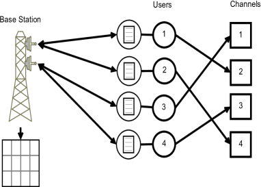
Figure 1: The System

II Problem Formulation

In our model, there are $N$ users that are served by a BS that has $K$ channels for allocation. Figure 1 depicts a toy example of our system with $K=N=4$. We assume that $K=bN$ for some positive integer $b$ and that each user is allocated $b$ channels. The parameter $b$, which we treat as given, can be optimized beforehand. A generalization of our analysis to a different number of channels per user is possible using a more cumbersome proof. We later demonstrate in simulations that our scheme works just as well in this case. Throughout the paper, we use calligraphic capitals to denote sets (and events), bold capitals to denote matrices and capitals or lower case letters to denote scalars. Our assumptions on the channel gains are as follows:

Channel Gains Assumptions

1. For each user $n$, the channel gains $g_{n,1},...,g_{n,K}$ are $K$ i.i.d. random variables. Channel gains of different users are independent. This is a widespread assumption in the channel allocation literature [14, 12, 13]. However, in contrast to [12, 13, 14, 11], we do not assume Rayleigh fading or that the channel gains of different users are identically distributed.

2. Each user can perfectly measure each of his $K$ channel gains. This widespread assumption [14, 12, 13, 27, 11, 26] is necessary so that each user can evaluate his $M$-best channels. In modern devices, multichannel sensing has become common practice that can be easily achieved by a beacon sent from the BS or other standard estimation techniques. Our approach does not require users to transmit this entire information to the BS.

3. Channel gains are quasi-static, such that the coherence time is larger than the time it requires to feed back the partial CSI (i.e., block-fading). This is also a very common assumption [14, 12, 13, 25, 11, 26, 10], since the multiuser diversity can only be exploited in scenarios where this assumption holds.

We assume that the transmission power is the same in each channel, so no water-filling technique is used. This assumption is later justified both analytically and in simulations that show that the water-filling gain is negligible in our model for all practical SNR values. This has been verified for many similar scenarios [18, 23, 19, 21, 22, 20].

Denote by $\mathcal{A}_{n}$ the set of allocated channels of user $n$. The achievable rates of the users in bits per channel use, $\left\{R_{n}\right\}$, are defined as

$$R_{n}\left(\mathcal{A}_{n}\right)=\sum_{k\in\mathcal{A}_{n}}\log_{2}\left(1+\frac{g_{n,k}^{2}P_{\max}}{bN_{0}}\right)$$ (1)

where $P_{\max}$ is the maximal transmission power of each user and $N_{0}$ is the variance of the Gaussian noise in his receiver. Often, the goal of a channel allocation scheme is to maximize the sum-rate of the users

$$\begin{array}[]{c}\underset{\left(\mathcal{A}_{1},...,\mathcal{A}_{N}\right)}{\max}\sum_{n=1}^{N}R_{n}\left(\mathcal{A}_{n}\right)\\ s.t.\,\,\mathcal{A}_{n}\bigcap\mathcal{A}_{m}=\emptyset\,\,\forall n,m\,,n\neq m\end{array}$$ (2)

where the constraint means that each channel is allocated to a single user (orthogonal transmission). However, maximizing the sum-rate often comes at the expense of fairness.

$$\begin{array}[]{c}\underset{\left(\mathcal{A}_{1},...,\mathcal{A}_{N}\right)}{\max}\underset{n}{\min}R_{n}\left(\mathcal{A}_{n}\right)\\ s.t.\,\,\mathcal{A}_{n}\bigcap\mathcal{A}_{m}=\emptyset\,\,\forall n,m\,,n\neq m\end{array}$$ (3)

Our goal is to design a limited feedback channel allocation scheme that maximizes the sum-rate without compromising the minimal-rate (fairness).

TABLE I: Notations and symbols used throughout this paper.

$N$	Number of users
$K$	Number of channels
$b$	Number of channels per user
$M$	Number of best channels for each user
$g_{n,k}$	Channel gain of user $n$ in channel $k$
$P_{\max}$	Maximal transmission power
$X_{\left(i\right)}$	The $i$-th smallest variable among $X_{1},...,X_{N}$
$\mathcal{E}_{K}$	Probability that a PM does not exist with $K$ channels

II-A Perfect Matching Allocation Scheme

In order for the BS to be able to compute the optimal solution of (2), all users need to feed back all their channel gains to the BS. Then, the optimal solution can be computed at the BS in polynomial time using the Hungarian Algorithm [33]. However, a feedback overhead of $K$ quantized numbers for each user renders this approach impractical for cellular networks. Therefore, suboptimal schemes with limited feedback overhead and good performance are essential.

In general, there is a fundamental tradeoff between the amount of feedback used for the allocation and the performance achieved. By choosing a specific feedback structure, one chooses a specific operating point for this tradeoff. For example, by feeding back the values of the $NK$ channel gains the optimal solution can be computed, and by feeding back one bit per user per channel ($K$ bits per user), state of the art thresholding schemes can be applied [10, 11, 12].

We propose a novel limited feedback scheme that requires less feedback than current state of the art schemes. Not only that it does not perform worse, it even performs much better. The scheme is summarized in Algorithm 1. In our approach, each user transmits only the indices of his $M$-best channels, without their numerical value. Feeding back the indices of the $M$-best channels was proposed in [14] for an opportunistic channel allocation scheme. The novelty of our approach is not in the feedback structure but in the fact that our approach is non-opportunistic. This means that all channels and all users are simultaneously considered in the computation of the allocation, and not one by one. In particular, only in our scheme the results of the next section about the optimal $M$ for a perfect matching (PM) are valid. Since [14] has nothing to do with perfect matchings, it suffers, like any opportunistic method, from an inherent non-fairness. We compare our performance to [14] in Section VI.

The information available at the BS using this limited feedback can be summarized using a bipartite graph defined as follows. Using this information, the BS aims to compute an allocation where each user gets $b$ of his $M$-best channels. Such an allocation does not necessarily exist, and the existence probability depends on $M$.

Definition II.1.

A user-channel graph $\Gamma$ is a balanced bipartite graph consisting of a user nodes set $\mathfrak{N}$ and a channel nodes set $\mathcal{\mathfrak{\mathcal{K}}}$. Every user $n\in\mathcal{N}$ has $b$ user nodes (“agents”) and every channel has a single channel node. An edge is connected between $n_{i}\in\mathfrak{N}$ and $k\in\mathcal{\mathfrak{\mathcal{K}}}$ if and only if channel $k$ is one of the $M$-best channels for user $n$. A PM allocation corresponds to a PM in this graph.

Algorithm 1 Perfect Matching Limited Feedback Scheme

Setting -There are $N$ users in a cell and $K=bN$ channels for a positive integer $b$. Let $g_{n,k}$ be the channel gain of user $n$ in channel $k$. Let $M=\left\lceil\left(1+b\right)\left(1+\varepsilon\right)\ln K\right\rceil$ for some $\varepsilon>0$.

Periodically in the cell:

1. The base-station (BS) broadcasts a common beacon on all $K$ channels.

2. Each user $n$ independently -

   1. Estimates the channel gains $g_{n,k}$ for each $k$.

   2. Transmits the subset of his $M$-best channels to the BS, using $\log_{2}\binom{K}{M}$ bits (see Algorithm 2).

3. Based on the information from 2(b), the BS constructs the bipartite graph $\Gamma$ of Definition II.1.

4. The BS computes the maximal matching in $\Gamma$ (e.g., using the algorithm of [30]).

5. The BS transmits to each user the channels he is matched to according to Step 4.

   1. Theorem III.1 guarantees that with high probability this matching will assign each user $b$ of his $M$-best channels (“perfect matching”).

   2. Theorem V.4 guarantees that with high probability this allocation will have asymptotically both optimal sum-rate and max-min fairness.

Algorithm 2 Feedback Encoding and Decoding

Encoding - The subset $\mathcal{S}\subset\left\{1,...,K\right\}$ is mapped to the index $E\left(\mathcal{S},K\right)$, defined recursively as

1. If $S=\emptyset$, then $E\left(\mathcal{S},K\right)=0$.

2. If $K$$\notin\mathcal{S}$, then $E\left(\mathcal{S},K\right)=E\left(\mathcal{S},K-1\right).$

3. If $K$$\in\mathcal{S}$, then $E\left(\mathcal{S},K\right)=\binom{K-1}{\left|\mathcal{S}\right|}+E\left(\mathcal{S}\setminus\left\{K\right\},K-1\right).$

Decoding - The index $e$ is mapped to the subset $D\left(e,K,M\right)$, defined recursively as

1. If $e=0$, then $D\left(0,K,M\right)=\emptyset$.

2. If $e<\binom{K-1}{M}$ then $D\left(e,K,M\right)=D\left(e,K-1,M\right)$.

3. If $e\geq\binom{K-1}{M}$ then $D\left(e,K,M\right)=D\left(e-\binom{K-1}{M},K-1,M-1\right)\bigcup\left\{K\right\}$.

From the perspective of the theory of random bipartite graphs, our graph is not typical. Each left side node has exactly $M$ edges whereas each right side node may have any degree. Additionally, groups of $b$ consecutive left side nodes are connected to the exact same right side nodes. In particular, this means that edge existence is not independent and that the graph is not an Erdős–Rényi graph. This is why a novel proof for the existence of a PM is needed.

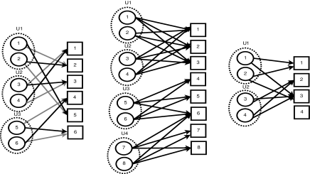
Figure 2: User-channel graphs.

Examples of user-channel graphs can be seen in Figure 2. In the left graph $N=3$, $b=2$ and $M=2$. A PM exists that consists of the grey edges. In the right most graph $N=2$, $b=2$ and $M=2$. No user is connected to channel 4 so no PM can exist. In the central graph, $N=4$, $b=2$ and $M=3$. Although each channel is connected to at least two user nodes, a PM does not exist. No matter which two channels are allocated to nodes 1 and 2, nodes 3 and 4 will be left with only one desired channel for both of them.

III Asymptotic Existence of PM Allocations

Our goal is to show that a PM allocation, where each user only gets $M$-best channels, exists. There is a trade-off for the parameter $M$. A large value of $M$ increases the probability that a PM allocation exists at the cost of reduced performance, since the $M$-best channel gets worse as $M$ increases. The feedback communication overhead also increases with $M$. Hence, it is important to identify the smallest value of $M$ for which a PM exists. In this section we characterize this optimal value of $M$ that is used in Algorithm 1.

The main theorem of this paper is stated as follows:

Theorem III.1 (Main Theorem).

Let $K=bN$ for a positive integer $b$ that is constant with respect to $N$. Let $\mathcal{E}_{K}$ be the event that a PM, where each user gets $b$ channels that are among his $M$-best, does not exist. If $M\geq\left(b+1\right)\left(1+\varepsilon\right)\ln K$ for some $\varepsilon>0$ then, for large enough $K$,

$$\Pr\left(\mathcal{E}_{K}\right)\leq\frac{1}{K^{\varepsilon+\frac{\varepsilon+1}{b}}}+\frac{\pi\sqrt{b}e^{3}}{12}\frac{1}{K^{\frac{3}{2}\varepsilon+\frac{\frac{3}{2}\varepsilon+1}{b}}}.$$ (4)

Thus, a PM exists with a probability that approaches one as $K\rightarrow\infty$. Furthermore, if $\varepsilon\geq 1$, then the indicator of $\mathcal{E}_{K}$ converges to zero almost surely.

Proof:

See Appendix A. ∎

For a PM to exist, every channel should be one of the $M$-best channels for at least one user. The following lemma shows that for this to occur, $M$ must increase with $K$ faster than $b\ln K$ and that $M=b\left(1+\varepsilon\right)\ln K$ is enough for that purpose.

Lemma III.2.

Let $K=bN$ for a positive integer $b$ that is constant with respect to $N$. Let $M>0$ and $\varepsilon>0$. Let $\mathcal{E}_{0}$ be the event that there is a channel which is not one of the $M$-best channels for any user.

1. If $M\leq b\ln K$ then $\underset{K\rightarrow\infty}{\lim}\Pr\left(\mathcal{E}_{0}\right)\geq\frac{1}{2}$.

2. If $M\geq b\left(1+\varepsilon\right)\ln K$ then $\underset{K\rightarrow\infty}{\lim}\Pr\left(\mathcal{E}_{0}\right)=0$.

Proof:

See Appendix A. ∎

IV Feedback Reduction

The implication of Theorem III.1 is that Algorithm 1 requires of each user to feed back only the indices of his $M=\left\lceil\left(b+1\right)\left(1+\varepsilon\right)\ln K\right\rceil$ best channels. This requires $\log_{2}\binom{K}{M}$ bits from each user, to encode a subset of size $M$ of a set of size $K$. Since $\log_{2}\binom{K}{M}\leq M\log_{2}K$, the amount of feedback bits per user per channel scales like $O\left(\frac{\log_{2}^{2}K}{K}\right)$, which improves with the number of channels $K$, therefore making our scheme especially appealing for large systems. In Algorithm 2 we present a practical method for encoding and decoding by indexing the subsets that requires exactly $\log_{2}\binom{K}{M}$ bits, used for the combinatorial number system [34]. Its computational complexity is $O\left(K\right)$.

Proposition IV.1.

The encoding of Algorithm 2 requires $\log_{2}\binom{K}{M}$ bits.

Proof:

The fact that $E\left(\mathcal{S},K\right)$ is a bijection so each subset has a unique index and vice versa is proven in [35]. For each subset $\mathcal{S}\subset\left\{1,...,K\right\}$ such that $\left|\mathcal{S}\right|=M$ we have

$$E\left(S,K\right)\leq\sum_{m=0}^{M}\binom{K-1-m}{M-m}\underset{\left(a\right)}{=}\binom{K}{M}$$ (5)

where (a) follows from the hockey-stick identity [35]. Hence, all the subsets $\mathcal{S}\subset\left\{1,...,K\right\}$ such that $\left|\mathcal{S}\right|=M$ are mapped by $E\left(\mathcal{S},K\right)$ to the indices 1 to $\binom{K}{M}$. ∎

State of the art limited feedback schemes [10, 11, 12] use a threshold for each channel gain. This means that each user has to send a packet of $K$ data bits in each coherence time of the channel (typically several milliseconds). Already in LTE $K=2048$ is a possibility [7], which results in a feedback (uplink) data rate of 409.6kbps for a coherence time of 5 milliseconds, more than four times the bandwidth of a voice call. In order to maintain multiuser diversity this feedback channel should be active very often. Besides creating a significant communication overhead in the uplink, this might not even be feasible due to battery constraints. Since the number of channels will increase in 5G systems, reducing the feedback amount is necessary if channel allocation with good performance is to be employed.

In general, in the high-SNR regime, the capacity of each user scales like $bB_{W}\ln\left(\ln N\right)$, where $B_{W}$ is the bandwidth of a channel and $\ln\left(\ln N\right)$ is from the multiuser diversity in Rayleigh fading channels [13]. For a thresholding method the feedback rate scales like $bN$, so the feedback becomes even larger than the data rate in large systems. In [13], it was suggested to mitigate this overhead by grouping channels, at the cost of a reduced sum-rate (and minimal rate). Our method requires a feedback rate that scales like $\ln^{2}N$ instead of like $N$ as the thresholding schemes. Therefore, for modern systems with a relatively large $B_{W}$, the feedback overhead of our scheme remains negligible even for very large values of $N$. Hence, our method achieves the necessary feedback reduction, not only without reducing the performance, but actually improving it. While the sum-rate improvement is moderate, the minimal rate is dramatically increased.

In Figure 3 we present the number of feedback bits our algorithm requires as a function of the number of channels $K$, for $b=1,4,8$ and $\varepsilon=0.3,0.7,0.8$, respectively. The values of $\varepsilon$ are chosen in order to minimize the number of feedback bits while keeping the probability that a PM does not exist sufficiently small. We also show the number of bits required by a naive encoding scheme that directly transmits the $M$ indices using $M\log_{2}K=\log_{2}K\left\lceil\left(b+1\right)\left(1+\varepsilon\right)\ln K\right\rceil$ bits. It is evident that our algorithm always requires less than the 1 bits per user per channel that state of the art thresholding approaches require [10, 11, 12]. In comparison, the optimal solution, given by the Hungarian algorithm, requires a quantization of $q$ bits per user per channel, where a reasonable $q$ that causes only a negligible performance degradation is $q=8$. For $N=256$ and $K=1024$, our approach requires less than 0.29 bits per user per channel - a saving of more than 70% in feedback overhead. For $K=2048$ this becomes a saving of more than 80%. Even for small values like $N=K=32$, our approach requires less than 0.8 bits per user per channel. We also present the upper bound of Theorem III.1 on the probability that a PM does not exist, which is always less than 2% and improves very fast as $K$ grows. Note that since the exponents of the bound in (4) are $\varepsilon+\frac{\varepsilon+1}{b}$ and $\frac{3}{2}\varepsilon+\frac{\frac{3}{2}\varepsilon+1}{b}$, the bound is much lower for $b=1$ and starts to behave like $\frac{1}{K^{\varepsilon}}$ for large $b$ values.

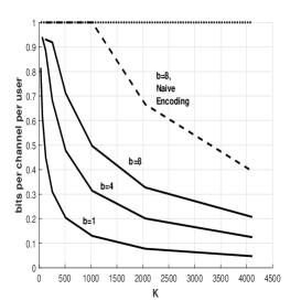
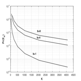
Figure 3: Number of bits for feedback in Algorithm 1, and the corresponding upper bound for the non-perfect matching probability.

V Asymptotic optimality of PM Allocations

In the previous section we showed that $M=\left(b+1\right)\left(1+\varepsilon\right)\ln K$, for some $\varepsilon>0$, is enough to guarantee that a PM allocation exists. In this section we show how good this PM allocation actually is. This has to do with the extent to which the $M$-best channel of each user is worse than his best channel. This definitely depends on the distribution of the channel gains. Luckily, all of the fading distributions used in practice tend to belong to the following class:

Definition V.1 (Exponentially-Dominated Tail Distribution).

Let $X$ be a random variable with a continuous CDF $F_{X}$. We say that $X$ has an exponentially-dominated tail distribution if there exist $\alpha>0,\beta\in\mathbb{R},\lambda>0,\gamma>0$ such that

$$\underset{x\rightarrow\infty}{\lim}\frac{1-F_{X}\left(x\right)}{\alpha x^{\beta}e^{-\lambda x^{\gamma}}}=1.$$ (6)

The following simple proposition validates that many commonly used fading distributions have an exponentially-dominated tail.

Proposition V.2.

The Rayleigh, $m$-Nakagami, Rice and Normal distributions are exponentially-dominated tail distributions.

Proof:

See Appendix A. ∎

The fact that each user gets $b$ of his $M$-best channels, and that $M$ is kept relatively small for exponentially-dominated fadings, provides both sum-rate and fairness guarantees. This is a special property of our allocation. In general, maximizing the sum-rate does not provide any fairness guarantees for the users, as demonstrated in the following example.

Example V.3.

Consider the following $K\times K$ rates matrix for the case of $b=1$, where $u_{n,k}$ is the rate of user $n$ in channel $k$. Let $\delta>0$ be a small number.

$$\boldsymbol{U}=\left(\begin{array}[]{ccccc}\delta&1&1&\cdots&1\\ 1&2&1&\cdots&1\\ \delta&1&1&\cdots&1\\ \vdots&\vdots&\vdots&\ddots&\vdots\\ \delta&1&1&\cdots&1\end{array}\right)$$

For this case, the Hungarian algorithm assigns channel $k$ to user $k$ for each $k$, resulting in a sum-rate of $K+\delta$ and a minimal rate of $\delta$. Our PM approach assigns each user one of his $M$-best channels. If $2\leq M\leq K-1$, our algorithm results in a sum-rate of $K$ and a minimal rate of $1$. For a small enough $\delta$, we obtain only a slight reduction in the sum-rate while having a dramatically better minimal rate.

The following theorem establishes the asymptotic optimality (in ratio) of a PM allocation both in the sum-rate and minimal rate senses, for exponentially-dominated tail fadings.

Theorem V.4 (Sum Rate and Fairness Optimality).

Let the channel gains be the i.i.d. variables $g_{n,1},...,g_{n,K}$ , for each $n$. If, for each $n$ and $k$, $g_{n,k}$ has an exponentially-dominated tail and $M=\left(b+1\right)(1+\varepsilon)\ln K$ for some $\varepsilon>0$, then

$$\operatorname*{plim}_{K\to\infty}\frac{\underset{\left(\mathcal{A}_{1},...,\mathcal{A}_{N}\right)\in\mathcal{P}}{\min}\sum_{n=1}^{N}R_{n}\left(\mathcal{A}_{n}\right)}{\underset{\left(\mathcal{A}_{1},...,\mathcal{A}_{N}\right)}{\max}\sum_{n=1}^{N}R_{n}\left(\mathcal{A}_{n}\right)}=1$$ (7)

where $\mathcal{P}$ is the set of PMs in the user-channel graph, and plim denotes convergence in probability. Furthermore,

$$\operatorname*{plim}_{K\to\infty}\frac{\underset{\left(\mathcal{A}_{1},...,\mathcal{A}_{N}\right)\in\mathcal{P}}{\min}\underset{n}{\min}R_{n}\left(\mathcal{A}_{n}\right)}{\underset{\left(\mathcal{A}_{1},...,\mathcal{A}_{N}\right)}{\max}\underset{n}{\max}R_{n}\left(\mathcal{A}_{n}\right)}=1.$$ (8)

Proof:

Denote by $g_{n,\left(i\right)}$ the $i$-th smallest channel gain among $g_{n,1},...,g_{n,K}$. Denote $\Phi=\left(\mathcal{A}_{1},...,\mathcal{A}_{N}\right)$. We have

$$1\geq\frac{\underset{\Phi\in\mathcal{P}}{\min}\sum_{n=1}^{N}R_{n}\left(\mathcal{A}_{n}\right)}{\underset{\Phi}{\max}\sum_{n=1}^{N}R_{n}\left(\mathcal{A}_{n}\right)}\underset{\left(a\right)}{\geq}\frac{\underset{\Phi\in\mathcal{P}}{\min}N\underset{n}{\min}R_{n}\left(\mathcal{A}_{n}\right)}{\underset{\Phi}{\max}N\underset{n}{\max}R_{n}\left(\mathcal{A}_{n}\right)}\underset{\left(b\right)}{\geq}\underbrace{\frac{\underset{n}{\min}b\log_{2}\left(1+\frac{g_{n,\left(K-M+1\right)}^{2}P_{\max}}{bN_{0}}\right)}{\underset{n}{\max}b\log_{2}\left(1+\frac{g_{n,\left(K\right)}^{2}P_{\max}}{bN_{0}}\right)}}_{A_{K}}\\ \geq\frac{\log_{2}\left(\left(1+\frac{\underset{n}{\max}g_{n,\left(K\right)}^{2}P_{\max}}{bN_{0}}\right)\frac{\underset{n}{\min}g_{n,\left(K-M+1\right)}^{2}}{\underset{n}{\max}g_{n,\left(K\right)}^{2}}\right)}{\log_{2}\left(1+\frac{\underset{n}{\max}g_{n,\left(K\right)}^{2}P_{\max}}{bN_{0}}\right)}=1+\underbrace{\frac{2\log_{2}\left(\frac{\underset{n}{\min}g_{n,\left(K-M+1\right)}}{\underset{n}{\max}g_{n,\left(K\right)}}\right)}{\log_{2}\left(1+\frac{\underset{n}{\max}g_{n,\left(K\right)}^{2}P_{\max}}{bN_{0}}\right)}}_{B_{K}}$$ (9)

where (a) follows since for every allocation, the sum-rate is larger than $N\underset{n}{\min}R_{n}\left(\mathcal{A}_{n}\right)$ and smaller than $N\underset{n}{\max}R_{n}\left(\mathcal{A}_{n}\right)$. Inequality (b) follows from the definition in (1) since each of the $b$ channel gains user $n$ gets is at least $\underset{n}{\min}\,g_{n,\left(K-M+1\right)}$ in all $\left(\mathcal{A}_{1},...,\mathcal{A}_{N}\right)\in\mathcal{P}$ and at most $\underset{n}{\max}\,g_{n,\left(K\right)}$ in all allocations. First note that for $g_{n,k}$ with a bounded distribution we have $\operatorname*{plim}_{K\to\infty}\frac{\underset{n}{\min}g_{n,\left(K-M+1\right)}}{\underset{n}{\max}g_{n,\left(K\right)}}=1$ since both the numerator and the denominator approach $F_{g}^{-1}\left(1\right)<\infty$, so $\operatorname*{plim}_{K\to\infty}B_{K}=0$. Theorem 7 in [32] uses an argument similar to (9) to show that $\operatorname*{plim}_{K\to\infty}A_{K}=1$ even if $g_{n,1},...,g_{n,K}$ are unbounded but have an exponentially-dominated tail, based on showing that $\operatorname*{plim}_{K\to\infty}\frac{\underset{n}{\min}g_{n,\left(K-M+1\right)}}{\underset{n}{\max}g_{n,\left(K\right)}}>0$ for exponentially-dominated tail distributions. Therefore (7),(8) are obtained from the Sandwich Theorem. ∎

Theorem V.4 has a stronger argument than simply asymptotic optimality of the sum-rate and the minimal rate. Observe that the denominator in (8) consists of the best rate a user can receive in any allocation, even an allocation that only favors him. This rate is achieved when user $n$ is allocated his best $b$ channels from out of the entire $K$ channels. Hence, even the user with the minimal rate, in all possible PM allocations, achieves asymptotically full multiuser diversity. In fact, this is also true for the $bN$ agents as well, which leads to the following corollary.

Corollary V.5.

Let $K=bN$ for a positive integer $b$ that is constant with respect to $N$. The ratio between the rate achieved by water-filling to that of an equal power allocation converges in probability to one as $K\rightarrow\infty$.

Proof:

Denote by $\left\{P_{n,k}^{*}\right\}$ the set of the optimal transmission powers given $\left\{g_{n,k}\right\}$. If $g_{n,k}$ is increased to $g_{n,\left(K\right)}$ for each $k$ and the transmission powers are kept as $P_{n,k}^{*}$ for each $k$, then the sum-rate increases. If for the increased channel gains the optimal power allocation is used instead of $\left\{P_{n,k}^{*}\right\},$ the sum-rate will further increase. The optimal power allocation for identical channel gains of $g_{n,\left(K\right)}$ is an equal power allocation. Using this argument, we obtain

$$\frac{\sum_{k\in\mathcal{A}_{n}}\log_{2}\left(1+\frac{g_{n,k}^{2}P_{\max}}{bN_{0}}\right)}{\sum_{k\in\mathcal{A}_{n}}\log_{2}\left(1+\frac{g_{n,k}^{2}P_{n,k}^{*}}{N_{0}}\right)}\underset{(a)}{\geq}\frac{\sum_{k\in\mathcal{A}_{n}}\log_{2}\left(1+\frac{g_{n,\left(K-M+1\right)}^{2}P_{\max}}{bN_{0}}\right)}{\sum_{k\in\mathcal{A}_{n}}\log_{2}\left(1+\frac{g_{n,\left(K\right)}^{2}P_{\max}}{bN_{0}}\right)}\geq\frac{\underset{n}{\min}\log_{2}\left(1+\frac{g_{n,\left(K-M+1\right)}^{2}P_{\max}}{bN_{0}}\right)}{\underset{n}{\max}\log_{2}\left(1+\frac{g_{n,\left(K\right)}^{2}P_{\max}}{bN_{0}}\right)}.$$ (10)

In (a) we also used $g_{n,k}\geq g_{n,\left(K-M+1\right)}$ for each $k$, which holds in a PM allocation with parameter $M$. ∎

VI Simulation Results

In this section, we demonstrate our analytical results using numerical simulations. We also validate the fact that our findings hold in a broader model that includes correlated channels and an allocation of unequal numbers of channels to users. All the rates are measured in bits per second, assuming that the bandwidth of a channel is 15kHz (as in LTE [36]). We used a Rayleigh fading network; i.e.,$\left\{g_{n,k}\right\}$ are Rayleigh distributed and $\left\{g_{n,k}^{2}\right\}$ are exponentially distributed. In each experiment, we ran 100 random realizations of the channel gains. Unless otherwise stated, the transmission powers were chosen such that the mean SNR for each link was 20dB. We used the Hungarian algorithm [33] to compute the optimal sum-rate solution. We computed the maximal matching in the bipartite graph (which Theorem 2 guarantees is a PM) using the algorithm in [28]. This algorithm requires a time complexity of $O\left(K\log_{2}^{2}K\right)$ instead of $O\left(K^{3}\right)$ for the Hungarian algorithm, which also could have been used for computing a maximal matching (on the binary preferences matrix).

VI-A Uncorrelated Identically-Distributed Channels

In this subsection, the channel gains were uncorrelated with parameter $\lambda=1$ for all exponential variables. We used the parameter $M=\left\lceil 1.5\left(b+1\right)\ln\left(K\right)\right\rceil$ and ran the simulations for $N=10,25,50,75,100$. We found that for every realization a PM existed. This implies that our asymptotic results are valid for as low as $N=10$.

In Figure 4, the mean and minimal rates are presented as a function of $N$ for $b=4$. It is evident that the performance of the PM allocation was already above 90% of the optimal allocation for $N=50$. As anticipated by our results, it improved with $N$. We can also see that the minimal rate of the optimal allocation was good, which was to be expected. The chance of a single user getting $b=4$ bad channels is smaller than in the case of $b=1$. The random allocation rates, which can be thought of as the result of an allocation that ignores the CSI, were far behind. This effect is crucial especially for the minimal rate. In [12], the BS assigns each channel to one of the users that exceeded a certain threshold (possibly with defined priorities between users). In order to make the algorithm competitive in the minimal rate sense as well, each time multiple users exceeded the threshold, we allocated the channel to the user with the minimal number of channels thus far. We used $b=4$, so $K=4N$. Our mean rate is slightly better than that of [12] for all $N\geq 20$. The minimal rate of [12] is much lower (~78% of our minimal rate), and does not increase with $N$ while our minimal rate does. Last but not least, we require $\frac{1}{K}\log_{2}\binom{K}{M}$ bits per user per channel (0.81 for $N=10$ and 0.52 for $N=200$), while [12] always requires one bit per user per channel (exceeded the threshold or not). Hence, our algorithm outperforms [12] both in terms of performance and feedback communication overhead.

In Figure 5, we compare our algorithm also to that of [14], which has two versions. This algorithm assigns a single channel to each user, so we had to choose $b=1$. We used the same $M=\left\lceil 3\ln\left(K\right)\right\rceil$ for our algorithm and that of [14]. The mean rate of the set-best version is very similar to ours, with exactly the same feedback communication overhead. The mean-rate in the ordered-best version is a little better than our mean-rate, but has a significant feedback cost. For $N=K=20$, the ordered-best requires ~2.25 bits per user per channel, while the set-best (and our approach) requires ~0.87 bits per user per channel. For $N=K=100$, the ordered-best requires ~0.98 bits per user per channel, while the set-best and our approach require ~0.55 bits per user per channel. However, our major anticipated advantage is in the minimal rate. The minimal rate of [14] is very close in both versions and is only about ~70% of our minimal rate, and decreases with $N$ while our minimal rate increases. The minimal rate of [12] converges to zero, since for $N=K$, the probability that some users will not be allocated a channel is high.

To show the tightness of our selected $M$ we now demonstrate the threshold phenomenon for the existence of a PM. In Table II, we present the empirical probability that a PM does not exist for both $M=\left\lfloor b\ln\left(K\right)\right\rfloor$ and $M=\left\lfloor 1.5\left(b+1\right)\ln\left(K\right)\right\rfloor$, with $b=4$, averaged over 10000 simulations. For $M=\left\lfloor b\ln\left(K\right)\right\rfloor$, already for $N=10$, the probability that a PM does not exist was close to 0.5 and monotonically increased with $N$. This is in agreement with Lemma III.2, that shows that for $M\leq b\ln\left(K\right)$ the probability that a PM does not exist is bounded from below by 0.5, for large enough $N$. For $M=\left\lfloor 1.5\left(b+1\right)\ln\left(K\right)\right\rfloor$, the empirical probability that a PM does not exist was much below the bound of Theorem III.1 for all $N$, but the gap between the two decreased with $N$. This is to be expected, since the proof of Theorem III.1 uses arguments that hold, and become tight, for large enough $N$.

In Figure 6, we present the rates as a function of $b$ for $N=30$. All the rates increased almost linearly with $b$, and the ratio of the rates of a PM allocation to the optimal allocation rates remained almost constant for all $b$. This implies that the results of Figure 4 are similar for each $b$ value.

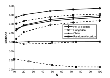
Figure 4: Achievable rates as a function of $N$ for uncorrelated channels. Solid lines represent the mean rates and dashed lines the minimal rates.

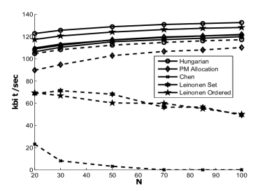
Figure 5: Achievable rates as a function of $N$ compared to Leinonen’s Algorithm, Chen’s Algorithm and the Hungarian Algorithm. Solid lines represent the mean rates and dashed lines the minimal rates.

TABLE II: Existence of PM allocations as a function of $N$ and $M$, for $b=4$.

$\Pr\left(\mathcal{E}_{bN}\right)$	$N=10$	$N=25$	$N=50$	$N=75$	$N=100$
$M=\left\lfloor b\ln\left(K\right)\right\rfloor$	0.44	0.52	0.54	0.65	0.67
$M=\left\lfloor 1.5(b+1)\ln\left(K\right)\right\rfloor$	0.004	0.004	0.004	0.004	0.003
$M=\left\lfloor 1.5(b+1)\ln\left(K\right)\right\rfloor$ upper bound	0.17	0.06	0.03	0.02	0.01

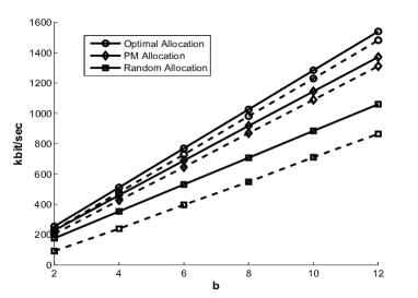
Figure 6: Achievable rates as a function of $b$ for $N=30$. Solid lines are used for the mean rates and dashed lines for the minimal rates.

VI-B Correlated Non-Identically Distributed Channels

In this subsection, we used correlated resource blocks as the channels, each consisting of 12 subcarriers. The rates are normalized per subcarrier. We used the Extended Pedestrian A model (EPA, see [36]) for the excess tap delay and the relative power of each tap. In this model, the channel gains of different users are not identically distributed, which is the practical scenario. We used $N=32,64,96,128$.

Figure 7 shows the mean and minimal rates as a function of $N$ averaged over 100 realizations for $b=4$. With correlated channels the diversity decreases; namely, adjacent channels are likely to be good or bad together. This makes the multiuser diversity gain lower and as a result the rates are lower, and look like the rates of the uncorrelated fading for smaller values of $N$. Additionally, this reduced diversity lead us to choose $M=\left\lceil 2\left(b+1\right)\ln\left(K\right)\right\rceil$, since a higher $M$ is needed for a PM to exist in the correlated user-channel graph. Indeed, we always found PMs for this choice of $M$. However, a larger $M$ makes the PM allocation rates lower. Nevertheless, these rates are still more than 85% of optimal rates already for $N=50$ and get closer as $N$ increases. Given these experimental results, we conjecture that our analytical results can be extended to the case of correlated channels.

In Figure 8, we repeated the above experiment with $b=1$ and a comparison to [14] and [12]. Note that both [14] and [12] assumed uncorrelated channels and identically distributed channel gains. In a thresholding approach, a different threshold can be used for each user, compromising mean-rate for fairness. However, since the minimal rate of [12] converges to zero anyway, we chose the threshold in order to optimize the mean-rate. As shown, the results are similar to those of Figure 5, and the feedback overhead comparison is of course the same. The main difference is that the minimal rate of all methods is lower. This does not represent a degradation for any of the algorithms, since with non-identically distributed channel gains, the minimal rate user is the user with the worst global conditions. In our method, the minimal rate is still significantly better than those of [14] and [12], since this minimal rate user got one of his best channels (even though all of them were relatively bad).

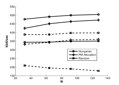
Figure 7: Achievable rates as a function of $N$ for non-identically distributed correlated channels. Solid lines represent the mean rates and dashed lines the minimal rates.

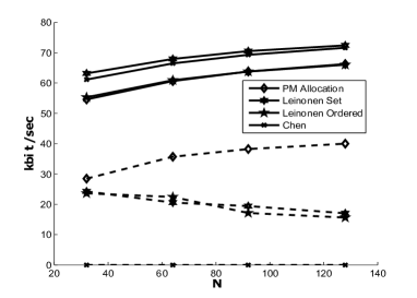
Figure 8: Achievable rates as a function of $N$ for non-identically distributed correlated channels, compared to state of the art algorithms. Solid lines represent the mean rates and dashed lines the minimal rates.

VI-C Unequal Channel Allocation

In this subsection, we allocated users a different number of channels, by dividing them into four classes. Specifically, $\frac{N}{4}$ of the users were allocated a single channel, $\frac{N}{4}$ two channels, $\frac{N}{4}$ three channels and $\frac{N}{4}$ four channels. We used $M=\left\lceil 3.75\ln\left(K\right)\right\rceil$ for all users, which amounts to using the average $b$ in $M=\left\lceil 1.07\left(b+1\right)\ln\left(K\right)\right\rceil$. Such a differentiation might occur if different users require a different quality of service (QoS). We simulated 100 realizations for each value from $N=12,20,48,72,100$. PMs still existed in all realizations. We ran another 100 realizations with correlated resource blocks, in the same manner as in Figure 7 and used $M=\left\lceil 5\ln\left(K\right)\right\rceil$ for all users. Figure 9 shows the empirical CDFs of the rates for the four classes, for uncorrelated channels and correlated resource blocks, with $N=100$ and $N=128$. Note that the PM allocation rates are quite concentrated and most of the users from the same class get similar rates. These rates are always better than those of a random allocation, and close to the optimal allocation rates. These results confirm our belief that our analysis can be generalized to the case of an unequal allocation, which is further supported by our proof itself.

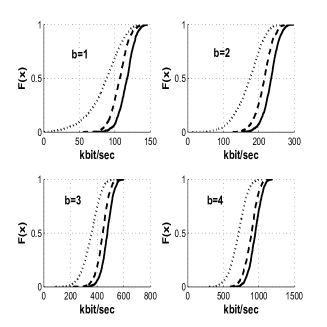
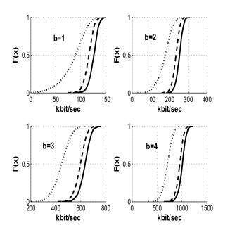
Figure 9: Empirical CDFs of the rates for different classes of users with $N=100$, for uncorrelated channels (left) and with $N=128$, for correlated resource blocks (right). Solid lines are used for optimal rates, dashed lines for the PM allocation rates and dotted lines for the random allocation rates.

VI-D Water-Filling Gain

In all the above results, water-filling over the $b$ channels of each user had a negligible gain. To be exact, it never improved any of the rates by more than 0.01 kbps. This is consistent with our analytical result in Corollary V.5. We repeated our experiment for an SNR of 10dB, $N=30$ and $M=\left\lceil 2\left(b+1\right)\ln\left(K\right)\right\rceil$, where the water-filling gain should be more significant than with our original parameters. We used $b=2,4,6,8,10,12,14$. In Figure 10 we present the water filling relative mean-rate gain, defined as $\frac{R_{WF}-R}{R}$, as a function of $b$. Clearly, even with an SNR of 10dB, water-filling did not improve the mean rates by more than 0.16% for either the Hungarian algorithm or our PM allocation for any $b$.

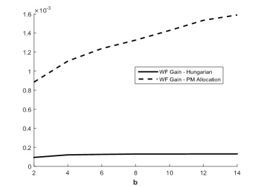
Figure 10: The water-filling relative mean-rate gain $\frac{R_{WF}-R}{R}$ as a function of $b$ for $N=30$ and an SNR of 10dB.

VII Conclusions

In this paper we suggested an approach aimed at achieving the multiuser diversity gain for resource block allocation under the frequency-selective channel. Our approach requires knowledge of the indices of the $M$-best channels for each of the $N$ users, instead of the whole $NK$ channel gains.

We showed that $M=\left(b+1\right)\left(1+\varepsilon\right)\ln\left(K\right)$ for some $\varepsilon>0$ guarantees that a PM allocation, where each user gets all his $b$ channels from his $M$-best channels, asymptotically exists. For this value of $M$, our suboptimal approach was shown to be asymptotically optimal for a broad class of fading distributions, both in the sum-rate and max-min senses.

Our algorithm is the first limited feedback algorithm that has provably asymptotic optimality both of the sum-rate and the minimal rate. It also requires significantly less feedback than the state of the art algorithms that achieve a good sum-rate. Hence, it constitutes a major step toward achieving the multiuser diversity gain of a selective channel in practice.

A future direction could involve trying to lift the assumption of i.i.d. channel gains by only assuming $m$-dependent channel gains and using the techniques presented in [37].

Appendix A Proofs

For our results, we need the following two lemmas.

Lemma A.1.

For each $0\leq l\leq K$ and $0\leq M\leq l$ we have $\frac{\binom{l}{M}}{\binom{K}{M}}\leq\left(\frac{l}{K}\right)^{M}$.

Proof:

$$\binom{l}{M}\binom{K}{M}^{-1}=\frac{\frac{l!}{\left(l-M\right)!}}{\frac{K!}{\left(K-M\right)!}}=\prod\limits_{i=1}^{M}\frac{l-M+i}{K-M+i}=\prod\limits_{j=0}^{M-1}\frac{l-j}{K-j}\underset{(a)}{\leq}\left(\frac{l}{K}\right)^{M}$$ (11)

where (a) follows since if $l<K$ then $f\left(x\right)=\frac{l-x}{K-x}$ is monotonically decreasing for all $x<K$, so $\frac{l-j}{K-j}\leq\frac{l}{K}$ for each $0\leq j<M$. ∎

Lemma A.2.

Let $M=\left(b+1\right)\left(1+\varepsilon\right)\ln K$ for some $\varepsilon>0$. Define the function

$$f\left(x\right)=K\left(1+\frac{1}{b}\right)h_{b}\left(\frac{x+1}{K}\right)\ln 2-\frac{M}{Kb}\left(K-x\right)\left(x+1\right)$$ (12)

where $h_{b}$ is the binary entropy function (see [38, page 666]). Then, for large enough $K$, we have for all $M\leq x\leq K-1$

$$f\left(x\right)\leq 3-\left(1+\frac{1}{b}\right)\left(1+\frac{3}{2}\varepsilon\right)\ln K$$ (13)

Proof:

Since $\frac{dKh_{b}\left(\frac{x+1}{K}\right)}{dx}=\log_{2}\left(\frac{K}{x+1}-1\right)$ we have

$$\frac{df\left(x\right)}{dx}=\left(1+\frac{1}{b}\right)\ln\left(\frac{K}{x+1}-1\right)-\frac{M}{b}\left(1-\frac{1}{K}\right)+\frac{2}{b}x\frac{M}{K}$$ (14)

and

$$\frac{d^{2}f\left(x\right)}{dx^{2}}=-\frac{1+\frac{1}{b}}{K-x-1}-\frac{1+\frac{1}{b}}{x+1}+\frac{2}{b}\frac{M}{K}.$$ (15)

so for any $x\in\left[\frac{\left(b+1\right)K}{M}-1,K-\frac{\left(b+1\right)K}{M}-1\right]$ we have $\frac{d^{2}f\left(x\right)}{dx^{2}}\geq 0$. For $K-\frac{\left(b+1\right)K}{M}-1\leq x\leq K-2$ we have

$$\frac{df\left(x\right)}{dx}\geq\left(1-\frac{2b+2}{M}-\frac{1}{K}\right)\frac{M}{b}-\left(1+\frac{1}{b}\right)\ln\left(K-1\right)\underset{\left(a\right)}{\geq}0$$ (16)

where (a) follows for $M=\left(b+1\right)\left(1+\varepsilon\right)\ln\left(K\right)$ and a large enough $K$. For $M\leq x\leq\frac{\left(b+1\right)K}{M}-1$ we have

$$\frac{df\left(x\right)}{dx}\leq\left(1+\frac{1}{b}\right)\ln\left(\frac{K}{M}-1\right)-\frac{M}{b}\left(1-\frac{1}{K}\right)+2+\frac{2}{b}\underset{\left(a\right)}{\leq}0.$$ (17)

where (a) holds for $M=\left(b+1\right)\left(1+\varepsilon\right)\ln\left(K\right)$ and a large enough $K$. Thus, $f\left(x\right)$ is convex in $\left[\frac{\left(b+1\right)K}{M}-1,K-\frac{\left(b+1\right)K}{M}-1\right]$, increasing in $\left[K-\frac{\left(b+1\right)K}{M}-1,K-2\right]$ and decreasing in $\left[M,\frac{\left(b+1\right)K}{M}-1\right]$. Hence, the maximum of $f\left(x\right)$ must be attained at the borders $l=M,K-2$. Observe that for all $l<\frac{K}{2}$

$$Kh_{b}\left(\frac{l}{K}\right)=l\log_{2}\frac{K}{l}-\left(K-l\right)\log_{2}\left(1-\frac{l}{K}\right)\underset{(a)}{\leq}2l+l\log_{2}\frac{K}{l}$$ (18)

where in (a) we used $\log_{2}\left(1-\frac{l}{K}\right)\geq-\frac{2l}{K}$ which is true for $l\leq\frac{K}{2}$. Now we substitute $x=M,K-2$ in $f\left(x\right)$ to obtain

$$f\left(M\right)\underset{(a)}{\leq}\left(1+\frac{1}{b}\right)\left(2\left(M+1\right)\ln 2+\left(M+1\right)\ln\frac{K}{M+1}\right)-\frac{M^{2}}{b}\left(1-\frac{1}{K}\right)+\frac{M^{3}}{bK}-\frac{M}{b}\underset{(b)}{\leq}\\ M\left(1+\frac{1}{b}\right)\left(3+\left(1+\frac{1}{M}\right)\ln K-\frac{M}{b+1}\left(1-\frac{1}{K}\right)\right)$$ (19)

where (a) is from (18) and (b) is for large enough $K$ due to $M=\left(b+1\right)\left(1+\varepsilon\right)\ln\left(K\right)$. Next

$$f\left(K-2\right)\underset{\left(a\right)}{=}\ln\left(2\right)\left(1+\frac{1}{b}\right)Kh_{b}\left(\frac{1}{K}\right)-\frac{M}{b}\frac{\left(K-1\right)\left(K-2\right)}{K}+\frac{M}{b}\frac{\left(K-2\right)^{2}}{K}-\frac{M}{b}\underset{(b)}{\leq}\\ \left(1+\frac{1}{b}\right)\ln 4K-\frac{2M}{b}\left(1-\frac{1}{K}\right)$$ (20)

where (a) is from $h_{b}\left(1-\frac{1}{K}\right)=h_{b}\left(\frac{1}{K}\right)$ and (b) from (18). Hence for large enough $K$ (20) is larger than (19). We conclude that for all $M\leq x\leq K-1$

$$f\left(x\right)\leq\underset{x}{\max}f\left(x\right)\leq\left(1+\frac{1}{b}\right)\ln 4K-\frac{2M}{b}\left(1-\frac{1}{K}\right)\\ \leq 3-\left(1+\frac{1}{b}\right)\ln K\left(2\left(1+\varepsilon\right)\left(1-\frac{1}{K}\right)-1\right)\underset{(a)}{\leq}3-\left(1+\frac{1}{b}\right)\left(1+\frac{3}{2}\varepsilon\right)\ln K$$ (21)

where (a) is true for large enough $K$ such that $\frac{1}{K}\leq\frac{1}{4}\frac{\varepsilon}{1+\varepsilon}$. ∎

A-A Proof of Theorem III.1

Proof:

The bipartite graph can also be represented using a $K\times K$ preferences matrix $U$. Our matrix $U$ is a simplified binary matrix where $u_{n,k}=0$ if channel $k$ is one of the $M$-best channels of agent $n$ and $u_{n,k}=1$ otherwise. It consists of $\frac{K}{b}$ submatrices of $b$ identical rows each, and exactly $M$ zeros at each row. We want to show that the probability that the Hungarian algorithm on $U$ converges after one iteration approaches one as $K\rightarrow\infty$; hence the resulting cost is zero, which represents a PM in the equivalent bipartite graph. Note that since $K=bN$ for a positive integer $b$, when $K\rightarrow\infty$ then also $N\rightarrow\infty$. Denote by $Q_{l}\left(K,M\right)$ the probability that $U$ can be covered by $K-l-1$ rows and $l$ columns such that all its zeros are covered, and that there is no smaller $l$ with this property. We want to upper bound $Q_{l}\left(K,M\right)$ for each $l$. Now observe that if $U$ is covered such that a row is covered but one of its identical rows is not, this means that $U$ could be covered without this row cover. Hence, if the row covers do not include all the identical rows, they are redundant. This means that only values of $K-l-1$ (or $l+1$) that are a multiple of $b$ should be considered, and $Q_{l}\left(K,M\right)=0$ for all other values. We proceed by counting the number of combinations of each such matrix

$$Q_{l}\left(K,M\right)\leq\underbrace{\binom{K}{l}\binom{\frac{K}{b}}{\frac{l+1}{b}}}_{A}\underbrace{\binom{K}{M}^{\frac{K-l-1}{b}}}_{B}\underbrace{\binom{l}{M}^{\frac{l+1}{b}}}_{C}\binom{K}{M}^{-\frac{K}{b}}=\binom{K}{l}\binom{\frac{K}{b}}{\frac{l+1}{b}}\left(\frac{\binom{l}{M}}{\binom{K}{M}}\right)^{\frac{l+1}{b}}$$ (22)

where $A$ is the number of combinations for the index of the $K-l-1$ covered rows and the $l$ covered columns. Now we have to count the combinations for the structure of the covered and uncovered rows. The factor $B$ is the number of combinations for $K-l-1$ covered rows with exactly $M$ zeros in each. We are left with $l+1$ rows that we know can be covered by $l$ columns, and no less than $l$. Hence each of these rows has zeros only in these $l$ columns, so there can be no more than $C$ such rows. Finally, the denominator $\binom{K}{M}^{\frac{K}{b}}$ is the number of combinations of a matrix with $M$ zeros in each row and $b$ duplicates of each such row, that constitute the whole probability space.

For $l=K-1$ we get

$$Q_{K-1}\left(K,M\right)\underset{(a)}{\leq}K\left(1-\frac{1}{K}\right)^{\frac{M}{b}K}\underset{(b)}{\leq}Ke^{-\frac{M}{b}}$$ (23)

where (a) follows from Lemma A.1 and (b) from the inequality $\left(1-\frac{1}{K}\right)^{K}\leq e^{-1}$. Note that for $l=1,...,M-1$ it is trivial that $Q_{l}\left(K,M\right)=0$ since each row has exactly $M$ zeros. For the rest of the proof we assume that $M<l\leq K-2$. For these values, we have

$$\binom{K}{l}\binom{\frac{K}{b}}{\frac{l+1}{b}}=\frac{l+1}{K-l}\binom{K}{l+1}\binom{\frac{K}{b}}{\frac{l+1}{b}}\underset{(a)}{\leq}\frac{\sqrt{b}}{2\pi}\frac{1}{\left(K-l\right)\left(1-\frac{l+1}{K}\right)}2^{K\left(1+\frac{1}{b}\right)h_{b}\left(\frac{l+1}{K}\right)}$$ (24)

where in (a) we used $\binom{K}{l}\leq\sqrt{\frac{1}{2\pi l\left(1-\frac{l}{K}\right)}}2^{Kh_{b}\left(\frac{l}{K}\right)}$, which is valid for all $0<l<K$ (where $h_{b}$ is the binary entropy function, see [38, page 666]). Combining the above we obtain from (22) the following upper bound

$$Q_{l}\left(K,M\right)\underset{(a)}{\leq}\frac{\sqrt{b}2^{K\left(1+\frac{1}{b}\right)h_{b}\left(\frac{l+1}{K}\right)}}{2\pi\left(K-l\right)\left(1-\frac{l+1}{K}\right)}\left(\frac{l}{K}\right)^{\frac{M}{b}\left(l+1\right)}\underset{(b)}{\leq}\frac{\sqrt{b}}{2\pi\left(K-l\right)\left(1-\frac{l+1}{K}\right)}e^{\ln\left(2\right)K\left(1+\frac{1}{b}\right)h_{b}\left(\frac{l+1}{K}\right)-\frac{M}{Kb}\left(K-l\right)\left(l+1\right)}$$ (25)

where (a) is due to Lemma A.1 and (24) and (b) is due to $1-\frac{K-l}{K}\leq e^{-\frac{K-l}{K}}$. We want to find the maximal value of this bound as a function of $l$. Define the auxiliary function $f\left(x\right)$ as in (12) and denote by $\mathcal{E}_{K}$ the event in which a PM does not exist. We conclude by the union bound that

$$\Pr\left(\mathcal{E}_{K}\right)\leq Q_{K-1}\left(K,M\right)+\sum_{l=M}^{K-2}Q_{l}\left(K,M\right)\leq Ke^{-\frac{M}{b}}+\sum_{l=M}^{K-2}\frac{\sqrt{b}K}{2\pi\left(K-l\right)\left(K-l-1\right)}e^{f\left(l\right)}\underset{\left(a\right)}{\leq}\\ Ke^{-\frac{M}{b}}+\frac{\frac{\sqrt{b}}{2\pi}e^{3}}{K^{\frac{3}{2}\varepsilon+\frac{\frac{3}{2}\varepsilon+1}{b}}}\sum_{l=M}^{K-2}\frac{1}{\left(K-l-1\right)^{2}}\underset{(b)}{\leq}Ke^{-\frac{M}{b}}+\frac{\frac{\sqrt{b}}{2\pi}e^{3}}{K^{\frac{3}{2}\varepsilon+\frac{\frac{3}{2}\varepsilon+1}{b}}}\sum_{k=1}^{\infty}\frac{1}{k^{2}}\underset{(c)}{\leq}\frac{1}{K^{\varepsilon+\frac{\varepsilon+1}{b}}}+\frac{\pi\sqrt{b}e^{3}}{12}\frac{1}{K^{\frac{3}{2}\varepsilon+\frac{\frac{3}{2}\varepsilon+1}{b}}}$$ (26)

where (a) follows from Lemma A.2 for large enough $K$, (b) follows by substituting $k=K-l-1$ and adding terms to the sum. Inequality (c) follows from (23) and $\sum_{k=1}^{\infty}\frac{1}{k^{2}}=\frac{\pi^{2}}{6}$. Note that if $\varepsilon\geq 1$ then $\sum_{K=1}^{\infty}\Pr\left(\mathcal{E}_{K}\right)<\infty$. Hence, by the Borel-Cantelli lemma, the probability that an infinite number of events from $\left\{\mathcal{E}_{K}\right\}$ will occur is zero. Hence, the indicator of $\mathcal{E}_{K}$ converges almost surely to zero. ∎

A-B Proof of Lemma III.2

Proof:

Let $\mathcal{E}_{0,k}$ be the event in which channel $k$ is not one of the $M$-best channels for any of the users. We bound from below and above the probability that there exists a channel that is not good for any of the users; i.e., the probability of $\mathcal{E}_{0}=\bigcup_{k}\mathcal{E}_{0,k}$. Due to the i.i.d. assumption on the channel gains and their independency between users we have $\Pr\left(\mathcal{E}_{0,k}\right)=\left(1-\frac{M}{K}\right)^{N}$. From the union bound we obtain that

$$\Pr\left(\mathcal{E}_{0}\right)=\Pr\left(\bigcup_{k}\mathcal{E}_{0,k}\right)\leq K\left(1-\frac{M}{K}\right)^{N}.$$ (27)

Since $\left(1-\frac{M}{K}\right)^{N}$ decreases with $M$, using $M\geq b\left(1+\varepsilon\right)\ln K$ leads to

$$\underset{K\rightarrow\infty}{\lim}\Pr\left(\mathcal{E}_{0}\right)\leq\underset{K\rightarrow\infty}{\lim}K\left(1-\frac{M}{K}\right)^{N}\leq\underset{K\rightarrow\infty}{\lim}K\left(1-\frac{b\left(1+\varepsilon\right)\ln K}{K}\right)^{\frac{K}{b}}=\underset{K\rightarrow\infty}{\lim}Ke^{-\left(1+\varepsilon\right)\ln K}=0.$$ (28)

Now we want to bound from above the probability of a PM. We do so by using the inclusion-exclusion principle. We use the following lower bound

$$\Pr\left(\bigcup_{k}\mathcal{E}_{0,k}\right)\geq\sum_{k}\Pr\left(\mathcal{E}_{0,k}\right)-\sum_{k_{1},k_{2}}\Pr\left(\mathcal{E}_{0,k_{1}}\bigcap\mathcal{E}_{0,k_{2}}\right).$$ (29)

By direct counting of the number of user-channel graphs with two undesired channels we obtain

$$\sum_{k_{1},k_{2}}\Pr\left(\mathcal{E}_{0,k_{1}}\bigcap\mathcal{E}_{0,k_{2}}\right)=\left(\begin{array}[]{c}K\\ 2\end{array}\right)\left(\begin{array}[]{c}K-2\\ M\end{array}\right)^{N}\left(\begin{array}[]{c}K\\ M\end{array}\right)^{-N}\underset{(a)}{\leq}\frac{K^{2}}{2}\left(1-\frac{2}{K}\right)^{M\frac{K}{b}}$$ (30)

since $\binom{K}{2}$ is the number of choices for these two channels, $\binom{K-2}{M}$ is the number of combinations of the edges of each agent and $\binom{K}{M}^{N}$ is the total number of user-channel graphs. Inequality (a) is from Lemma A.1. We obtain

$$\Pr\left(\mathcal{E}_{0}\right)=\Pr\left(\bigcup_{k}\mathcal{E}_{0,k}\right)\geq K\left(1-\frac{M}{K}\right)^{N}-\frac{K^{2}}{2}\left(1-\frac{2}{K}\right)^{M\frac{K}{b}}.$$ (31)

Obviously, $\Pr\left(\mathcal{E}_{0}\right)$ decreases with $M$. Hence, using $M=b\ln K$, we conclude that

$$\underset{K\rightarrow\infty}{\lim}\Pr\left(\mathcal{E}_{0}\right)\geq\underset{K\rightarrow\infty}{\lim}\left(K\underbrace{\left(1-\frac{b\ln K}{K}\right)^{\frac{K}{b}}}_{\rightarrow e^{-\ln K}}-\frac{K^{2}}{2}\underbrace{\left(1-\frac{2}{K}\right)^{K\ln K}}_{\rightarrow e^{-2\ln K}}\right)=\frac{1}{2}.$$ (32)

∎

A-C Proof of Proposition V.2

Proof:

For the Rayleigh distribution we have $F_{X}\left(x\right)=1-e^{-\frac{x^{2}}{2\sigma^{2}}}$, so we simply have $\frac{1-F_{X}\left(x\right)}{\alpha x^{\beta}e^{-\lambda x^{\gamma}}}=1$ for $\alpha=1$, $\beta=0$,$\gamma=2$ and $\lambda=\frac{1}{2\sigma^{2}}$. Denote the PDF by $f_{X}\left(x\right)$. From l’Hôpital’s [39, Page 109] rule we obtain

$$\underset{x\rightarrow\infty}{\lim}\frac{1-F_{X}\left(x\right)}{\alpha x^{\beta}e^{-\lambda x^{\gamma}}}=\underset{x\rightarrow\infty}{\lim}\frac{f_{X}\left(x\right)}{\left(\alpha\lambda\gamma-\frac{\alpha\beta}{x^{\gamma}}\right)x^{\beta-1+\gamma}e^{-\lambda x^{\gamma}}}.$$ (33)

For an $m$-Nakagami distribution with parameter $\Omega>0$, $f_{X}\left(x\right)=\frac{2m^{m}}{\Gamma\left(m\right)\Omega^{m}}x^{2m-1}e^{-\frac{m}{\Omega}x^{2}}$. Substituting $\alpha=\frac{m^{m-1}}{\Gamma\left(m\right)\Omega^{m-1}}$, $\beta=2m-2$,$\gamma=2$ and $\lambda=\frac{m}{\Omega}$ in (33) yields

$$\underset{x\rightarrow\infty}{\lim}\frac{\frac{2m^{m}}{\Gamma\left(m\right)\Omega^{m}}x^{2m-1}e^{-\frac{m}{\Omega}x^{2}}}{\left(\frac{2m^{m}}{\Gamma\left(m\right)\Omega^{m}}-\frac{\alpha\beta}{x^{2}}\right)x^{2m-1}e^{-\frac{m}{\Omega}x^{2}}}=1.$$ (34)

For the Rice distribution (with an expectation shifted by a constant $v$) $f_{X}\left(x\right)=f_{Y}\left(x+v\right)=\frac{x+v}{\sigma^{2}}e^{-\frac{\left(x+v\right)^{2}+v^{2}}{2\sigma^{2}}}I_{0}\left(\frac{\left(x+v\right)v}{\sigma^{2}}\right)$. Substituting $\alpha=\sigma\sqrt{\frac{1}{2\pi v}}$, $\beta=-\frac{1}{2}$,$\gamma=2$ and $\lambda=\frac{1}{2\sigma^{2}}$ in (33) yields

$$\underset{x\rightarrow\infty}{\lim}\frac{\frac{x+v}{\sigma^{2}}e^{-\frac{\left(x+v\right)^{2}+v^{2}}{2\sigma^{2}}}I_{0}\left(\frac{\left(x+v\right)v}{\sigma^{2}}\right)}{\left(\frac{1}{\sigma}\sqrt{\frac{1}{2\pi v}}+\frac{\alpha}{2x^{2}}\right)\sqrt{x}e^{-\frac{x^{2}}{2\sigma^{2}}}}\underset{(a)}{=}\underset{x\rightarrow\infty}{\lim}\frac{\sqrt{x+v}}{\sqrt{x}}=1$$ (35)

where (a) follows since $\underset{x\rightarrow\infty}{\lim}\frac{I_{0}\left(\frac{xv}{\sigma^{2}}\right)}{\frac{\sigma}{\sqrt{2\pi xv}}e^{\frac{xv}{\sigma^{2}}}}=1$. For a Gaussian distribution $f_{X}\left(x\right)=\frac{1}{\sqrt{2\pi\sigma^{2}}}e^{-\frac{1}{2\sigma^{2}}x^{2}}$. Substituting $\alpha=\sqrt{\frac{\sigma^{2}}{2\pi}}$, $\beta=-1$,$\gamma=2$ and $\lambda=\frac{1}{2\sigma^{2}}$ in (33) yields

$$\underset{x\rightarrow\infty}{\lim}\frac{\frac{1}{\sqrt{2\pi\sigma^{2}}}e^{-\frac{1}{2\sigma^{2}}x^{2}}}{\left(\frac{1}{\sqrt{2\pi\sigma^{2}}}+\frac{\alpha}{x^{2}}\right)e^{-\frac{1}{2\sigma^{2}}x^{2}}}=1.$$ (36)

∎

References

- [1] I. Bistritz and A. Leshem, “Efficient and asymptotically optimal resource block allocation,” in 2018 IEEE Wireless Communications and Networking Conference (WCNC). IEEE, 2018, pp. 1–6.
- [2] Q. Zhao and B. M. Sadler, “A survey of dynamic spectrum access,” Signal Processing Magazine, IEEE, vol. 24, no. 3, pp. 79–89, 2007.
- [3] M. Hasan, E. Hossain, and D. Niyato, “Random access for machine-to-machine communication in LTE-advanced networks: issues and approaches,” IEEE Communications Magazine, vol. 51, no. 6, pp. 86–93, 2013.
- [4] K. Akkarajitsakul, E. Hossain, D. Niyato, and D. I. Kim, “Game theoretic approaches for multiple access in wireless networks: A survey,” IEEE Communications Surveys & Tutorials, vol. 13, no. 3, pp. 372–395, 2011.
- [5] K. Seong, M. Mohseni, and J. M. Cioffi, “Optimal resource allocation for OFDMA downlink systems,” in 2006 IEEE International Symposium on Information Theory, 2006.
- [6] W. Zhao, S. Wang, and J. Guo, “Efficient resource allocation for OFDMA-based device-to-device communication underlaying cellular networks,” in Communications in China (ICCC), 2015 IEEE/CIC International Conference on, 2015.
- [7] A. Ghosh, J. Zhang, J. G. Andrews, and R. Muhamed, Fundamentals of LTE. Pearson Education, 2010.
- [8] T. Yoo and A. Goldsmith, “Optimality of zero-forcing beamforming with multiuser diversity,” in Communications, 2005. ICC 2005. 2005 IEEE International Conference on, 2005.
- [9] J.-C. Guey and L. D. Larsson, “Modeling and evaluation of MIMO systems exploiting channel reciprocity in TDD mode,” in Vehicular Technology Conference, 2004. VTC2004-Fall. 2004 IEEE 60th, vol. 6, 2004, pp. 4265–4269.
- [10] D. Gesbert and M.-S. Alouini, “How much feedback is multi-user diversity really worth?” in Communications, 2004 IEEE International Conference on, vol. 1, 2004, pp. 234–238.
- [11] S. Sanayei and A. Nosratinia, “Opportunistic downlink transmission with limited feedback,” IEEE Transactions on Information Theory, vol. 53, no. 11, pp. 4363–4372, 2007.
- [12] J. Chen, R. A. Berry, and M. L. Honig, “Large system performance of downlink OFDMA with limited feedback,” in Information Theory, 2006 IEEE International Symposium on, 2006, pp. 1399–1403.
- [13] ——, “Limited feedback schemes for downlink OFDMA based on sub-channel groups,” IEEE Journal on Selected Areas in Communications, vol. 26, no. 8, pp. 1451–1461, 2008.
- [14] J. Leinonen, J. Hämäläinen, and M. Juntti, “Performance analysis of downlink OFDMA resource allocation with limited feedback,” IEEE Transactions on Wireless Communications, vol. 8, no. 6, pp. 2927–2937, 2009.
- [15] P. Erdos and A. Renyi, “On random matrices,” Magyar Tud. Akad. Mat. Kutató Int. Közl, vol. 8, no. 455-461, p. 1964, 1964.
- [16] E. Yaacoub and Z. Dawy, “A survey on uplink resource allocation in OFDMA wireless networks,” IEEE Communications Surveys & Tutorials, vol. 14, no. 2, pp. 322–337, 2012.
- [17] S. Sadr, A. Anpalagan, and K. Raahemifar, “Radio resource allocation algorithms for the downlink of multiuser OFDM communication systems,” IEEE Communications Surveys & Tutorials, vol. 11, no. 3, pp. 92–106, 2009.
- [18] L. M. Hoo, B. Halder, J. Tellado, and J. M. Cioffi, “Multiuser transmit optimization for multicarrier broadcast channels: asymptotic FDMA capacity region and algorithms,” IEEE Transactions on Communications, vol. 52, no. 6, pp. 922–930, 2004.
- [19] K. Kim, Y. Han, and S.-L. Kim, “Joint subcarrier and power allocation in uplink OFDMA systems,” IEEE Communications Letters, vol. 9, no. 6, pp. 526–528, 2005.
- [20] W. Yu and J. M. Cioffi, “Constant-power waterfilling: performance bound and low-complexity implementation,” IEEE Transactions on Communications, vol. 54, no. 1, pp. 23–28, 2006.
- [21] W. Yu, G. Ginis, and J. M. Cioffi, “Distributed multiuser power control for digital subscriber lines,” Selected Areas in Communications, IEEE Journal on, vol. 20, no. 5, pp. 1105–1115., 2002.
- [22] I. C. Wong and B. L. Evans, “Optimal downlink OFDMA resource allocation with linear complexity to maximize ergodic rates,” IEEE Transactions on Wireless Communications, vol. 7, no. 3, pp. 962–971, 2008.
- [23] J. Jang and K. B. Lee, “Transmit power adaptation for multiuser OFDM systems,” IEEE Journal on selected areas in communications, vol. 21, no. 2, pp. 171–178, 2003.
- [24] D. J. Love, R. W. Heath, V. K. Lau, D. Gesbert, B. D. Rao, and M. Andrews, “An overview of limited feedback in wireless communication systems,” IEEE Journal on selected areas in Communications, vol. 26, no. 8, pp. 1341–1365, 2008.
- [25] Y. S. Al-Harthi, A. H. Tewfik, and M.-S. Alouini, “Multiuser diversity with quantized feedback,” IEEE Transactions on Wireless Communications, vol. 6, no. 1, pp. 330–337, 2007.
- [26] I. Toufik and H. Kim, “MIMO-OFDMA opportunistic beamforming with partial channel state information,” in Communications, 2006. ICC’06. IEEE International Conference on, vol. 12, 2006, pp. 5389–5394.
- [27] P. Svedman, S. K. Wilson, L. J. Cimini, and B. Ottersten, “Opportunistic beamforming and scheduling for OFDMA systems,” IEEE Transactions on Communications, vol. 55, no. 5, pp. 941–952, 2007.
- [28] O. Naparstek and A. Leshem, “A fast matching algorithm for asymptotically optimal distributed channel assignment,” in Digital Signal Processing (DSP), 2013 18th International Conference on, 2013.
- [29] ——, “Fully distributed optimal channel assignment for open spectrum access,” IEEE Transactions on Signal Processing, vol. 62, no. 2, pp. 283–294, 2014.
- [30] ——, “Expected time complexity of the auction algorithm and the push relabel algorithm for maximum bipartite matching on random graphs,” in Random Structures & Algorithms. Wiley Online Library, 2014.
- [31] I. Bistritz and A. Leshem, “Asymptotically optimal distributed channel allocation: a competitive game-theoretic approach,” in Communication, Control, and Computing (Allerton), 2015 53nd Annual Allerton Conference on, 2015.
- [32] ——, “Game theoretic dynamic channel allocation for frequency-selective interference channels,” IEEE Transactions on Information Theory, 2018, DOI: 10.1109/TIT.2018.2868440.
- [33] C. H. Papadimitriou and K. Steiglitz, Combinatorial optimization: algorithms and complexity. Courier Corporation, 1998.
- [34] D. H. Lehmer, Applied Combinatorial Mathematics, E. F. Beckenbach, Ed. John Wiley & Sons, 1964.
- [35] A. B. Siddique, S. Farid, and M. Tahir, “Proof of bijection for combinatorial number system,” arXiv preprint arXiv:1601.05794. 2016.
- [36] LTE ETSI, “Evolved universal terrestrial radio access (e-utra); base station (bs) radio transmission and reception (3gpp ts 36.104 version 8.6. 0 release 8), july 2009,” ETSI TS, vol. 136, no. 104, p. V8, 2009.
- [37] I. Bistritz and A. Leshem, “Game theoretic resource allocation for m-dependent channel with application to OFDMA,” in Acoustics, Speech and Signal Processing (ICASSP), 2017 IEEE International Conference on, 2017, pp. 4316–4320.
- [38] T. M. Cover and J. A. Thomas, Elements of information theory. John Wiley & Sons, 2012.
- [39] W. Rudin et al., Principles of mathematical analysis. McGraw-hill New York, 1964.