FR-PHENO-2017-013, CP3-Origins-2017-045 DNRF90

Precision calculations for ${\mathrm{h}}\to{\mathrm{W}}{\mathrm{W}}/{\mathrm{Z}}{\mathrm{Z}}\to 4$ fermions
in the Two-Higgs-Doublet Model with Prophecy4f

Lukas Altenkamp¹, Stefan Dittmaier¹, Heidi Rzehak^2
1Albert-Ludwigs-Universität Freiburg, Physikalisches Institut,
79104 Freiburg, Germany
²University of Southern Denmark, $\text{CP}^{3}$-Origins
Campusvej 55, DK-5230 Odense M, Denmark

Abstract:

We have calculated the next-to-leading-order electroweak and QCD corrections to the decay processes ${\mathrm{h}}\to{\mathrm{W}}{\mathrm{W}}/{\mathrm{Z}}{\mathrm{Z}}\to 4\,$fermions of the light CP-even Higgs boson h of various types of Two-Higgs-Doublet Models (Types I and II, “lepton-specific” and “flipped” models). The input parameters are defined in four different renormalization schemes, where parameters that are not directly accessible by experiments are defined in the $\overline{\mathrm{MS}}$ scheme. Numerical results are presented for the corrections to partial decay widths for various benchmark scenarios previously motivated in the literature, where we investigate the dependence on the $\overline{\mathrm{MS}}$ renormalization scale and on the choice of the renormalization scheme in detail. We find that it is crucial to be precise with these issues in parameter analyses, since parameter conversions between different schemes can involve sizeable or large corrections, especially in scenarios that are close to experimental exclusion limits or theoretical bounds. It even turns out that some renormalization schemes are not applicable in specific regions of parameter space. Our investigation of differential distributions shows that corrections beyond the Standard Model are mostly constant offsets induced by the mixing between the light and heavy CP-even Higgs bosons, so that differential analyses of ${\mathrm{h}}\to 4f$ decay observables do not help to identify Two-Higgs-Doublet Models. Moreover, the decay widths do not significantly depend on the specific type of those models. The calculations are implemented in the public Monte Carlo generator Prophecy4f and ready for application.

October 2017

1 Introduction

The CERN Large Hadron Collider (LHC) was built to explore the validity of the Standard Model (SM) of particle physics at energy scales ranging from the electroweak scale $\sim$100 GeV up to energies of some TeV and to search for new phenomena and new particles in this energy domain. The discovery of a Higgs particle at LHC Run 1 in 2012 [1, 2] was a first big achievement in this enterprise. Since first studies of the properties of this Higgs particle (spin, CP parity, couplings to the heaviest SM particles) show good agreement between measurements and SM predictions, the SM is in better shape than ever to describe all known particle phenomena up to very few exceptions. Assuming the absence of spectacular new-physics signals in LHC data, this means that any deviation from the SM hides in small and subtle effects. To extract those differences from data, both experimental analyses and theoretical predictions have to be performed with the highest possible precision. On the other hand, assuming that a new signal materializes at the $5\sigma$ level, the properties of the newly discovered particle have to be investigated with precision, in order to tell different models apart that can accommodate the new phenomenon.

Most of the promising candidates for models beyond the SM modify or extend the scalar sector of electroweak (EW) symmetry breaking, which introduces the Higgs boson in the SM. Lacking clear evidence of the realization of a specific model extension, it is well motivated to prepare experimentally testable predictions within generic SM extensions which are building blocks in larger models. Two-Higgs-Doublet Models (THDMs) [3, 4], where a second Higgs doublet is added to the SM field content, provide an interesting class of such generic models. While the gauge structure of the SM is kept, THDMs contain five physical Higgs bosons in contrast to the one of the SM. Three out of the five are neutral and two are charged. In the CP-conserving case, considered in this paper, one of the neutral Higgs bosons is CP-odd and two are CP-even. An important issue in identifying or constraining a THDM, thus, consists in telling the SM Higgs boson from an SM-like CP-even Higgs boson of THDMs. To this end, several phenomenological studies in THDMs have been carried out recently by various groups [5, 6, 7, 8, 9, 10, 11, 12, 13, 14, 15, 16, 17, 18, 19, 20, 21].

In this paper we investigate the decay observables of the SM-like neutral, light, CP-even Higgs boson h decaying into four fermions, ${\mathrm{h}}\to{\mathrm{W}}{\mathrm{W}}/{\mathrm{Z}}{\mathrm{Z}}\to 4f$, in the THDM, including next-to-leading-order (NLO) corrections of the EW and strong interactions. The fermions in the final state of these processes can either be quarks or leptons, and especially the latter can be resolved very well in the detector. These four-body decays were already crucial in the Higgs-boson discovery, but also play a major role in precision studies of the Higgs boson, in particular, to determine the couplings to the EW gauge bosons W and Z. They also provide a window to physics beyond the SM [22, 23, 24, 25, 26, 27, 28, 29], as, due to its high precision, small deviations from the SM can be measured, and differential distributions can be investigated and tested against the SM. The Monte Carlo program Prophecy4f [30, 31, 32] performs the calculation of the full NLO EW and QCD corrections for all ${\mathrm{h}}\to{\mathrm{W}}{\mathrm{W}}/{\mathrm{Z}}{\mathrm{Z}}\to 4f$ channels in the complex-mass scheme [33, 34, 35] to describe the intermediate W- and Z-boson resonances. It provides differential distributions as well as unweighted events for leptonic final states. The corrections to ${\mathrm{h}}\to{\mathrm{Z}}{\mathrm{Z}}\to 4\,$leptons were also calculated and matched to a QED parton shower in Ref. [36]. In the following, we describe results obtained with an updated version of Prophecy4f, extended to the computation in the THDM in such a way that the usage of the program and its applicability as event generator basically remain the same.

It is our goal to analyze the Higgs decay in the context of the most relevant THDM scenarios. To compute phenomenologically relevant results, we need to take into account current constraints which also restrict the large parameter space. The constraints come from direct LHC searches for heavy Higgs bosons and from theoretical aspects like vacuum stability, perturbative unitarity, or perturbativity of the couplings, which are required for a meaningful perturbative evaluation. The recent report of the LHC Higgs Cross Section Working Group [37] summarizes a selection of relevant benchmark scenarios proposed in other papers among which we study the most relevant. The results are compared with the SM prediction, and deviations are quantified. In addition to the usual investigation of residual scale uncertainties, we compare the results of different renormalization schemes recently presented and discussed in the literature [38, 39, 40, 41]. Specifically, we employ the four different schemes described in Ref. [40] and vary the renormalization scale to investigate the perturbative stability of the predictions in the benchmark scenarios. Similar to what has already been found in the Minimal Supersymmetric SM [42], the different renormalization schemes may suffer from problems like gauge dependence, singularities in relations between parameters, or unnaturally large corrections. The comparison of the results obtained with different renormalization schemes allows us to determine regions where they behave well and yield reliable results. Electroweak corrections to other Higgs-boson decay channels in the THDM were investigated in Refs. [38, 43]. Generic tools to calculate Higgs decay widths in the THDM, such as Hdecay [44] and THDMC [45] are currently restricted to QCD corrections (see, e.g., Refs. [46, 47] for more details).

This paper is structured as follows: In Sec. 2 we briefly describe the program Prophecy4f, on which our implementation is based, and give some details on our NLO calculation of corrections to the ${\mathrm{h}}{\to}4f$ decays in the THDM, including a survey of Feynman diagrams, the salient features of the calculation, and a short outline of the implementation into Prophecy4f. In Sec. 3, we describe the setup of our numerical analysis and the chosen THDM scenarios. The numerical results are presented and discussed in detail in Sec. 4. We conclude in Sec. 5 and provide some supplementary results in the appendix.

2 Predicting ${\mathrm{h}}\to{\mathrm{W}}{\mathrm{W}}/{\mathrm{Z}}{\mathrm{Z}}\to 4f$ in the THDM with the Monte Carlo program Prophecy4f

2.1 Preliminaries and functionality of Prophecy4f

The Monte Carlo program Prophecy4f [30, 31, 32] provides a “PROPer description of the Higgs dECaY into 4 Fermions” by calculating the decay observables of the process ${\mathrm{h}}\to{\mathrm{W}}{\mathrm{W}}/{\mathrm{Z}}{\mathrm{Z}}\to 4f$ at NLO EW+QCD accuracy in the SM. The original Prophecy4f code contains the matrix elements of all 19 possible $4f$ final states, which are listed in Tab. 1, in a generic way. It takes into account the full off-shell effects of the intermediate W and Z bosons and treats the W- and Z-boson resonances in the complex-mass scheme [33, 34, 35], which maintains gauge invariance and NLO precision both in resonant and non-resonant phase-space regions. For the evaluation of the one-loop integrals in the virtual corrections we have replaced the original internal integral library by the publicly available Fortran library Collier [48]. Ultraviolet (UV) divergences are treated in dimensional regularization, while the (soft and collinear) infrared (IR) divergences of the loop integrals and in the real photon or gluon emission are regularized by small photon, gluon, and external fermion masses. The final-state fermions are considered in the massless limit, i.e. small fermion masses are only kept as regulators in the singular logarithms. However, in diagrams with a closed fermion loop the full mass dependence of those fermions is kept which allows to extend the calculation to include a heavy fourth fermion generation, as done in Ref. [50]. The cancellation of the IR divergences can be performed via phase-space slicing [51] or dipole subtraction [52, 53, 54].

Final states	leptonic	semi-leptonic	hadronic
neutral current	$\nu_{\mathrm{e}}\bar{\nu}_{\mathrm{e}}\nu_{\mu}\bar{\nu}_{\mu}$ (3)	$\nu_{\mathrm{e}}\bar{\nu}_{\mathrm{e}}{\mathrm{u}}\bar{{\mathrm{u}}}$ (6)	${\mathrm{u}}\bar{{\mathrm{u}}}{\mathrm{c}}\bar{{\mathrm{c}}}$ (1)
	${\mathrm{e}}^{-}{\mathrm{e}}^{+}\mu^{-}\mu^{+}$ (3)	$\nu_{\mathrm{e}}\bar{\nu}_{\mathrm{e}}{\mathrm{d}}\bar{{\mathrm{d}}}$ (9)	${\mathrm{d}}\bar{{\mathrm{d}}}{\mathrm{s}}\bar{{\mathrm{s}}}$ (3)
	$\nu_{\mathrm{e}}\bar{\nu}_{\mathrm{e}}\mu^{-}\mu^{+}$ (6)	${\mathrm{e}}^{-}{\mathrm{e}}^{+}{\mathrm{u}}\bar{{\mathrm{u}}}$ (6)	${\mathrm{u}}\bar{{\mathrm{u}}}{\mathrm{s}}\bar{{\mathrm{s}}}$ (4)
		${\mathrm{e}}^{-}{\mathrm{e}}^{+}{\mathrm{d}}\bar{{\mathrm{d}}}$ (9)
neutral current with interference	${\mathrm{e}}^{-}{\mathrm{e}}^{+}{\mathrm{e}}^{-}{\mathrm{e}}^{+}$ (3)		${\mathrm{u}}\bar{{\mathrm{u}}}{\mathrm{u}}\bar{{\mathrm{u}}}$ (2)
	$\nu_{\mathrm{e}}\bar{\nu}_{\mathrm{e}}\nu_{\mathrm{e}}\bar{\nu}_{\mathrm{e}}$ (3)		${\mathrm{d}}\bar{{\mathrm{d}}}{\mathrm{d}}\bar{{\mathrm{d}}}$ (3)
charged current	$\nu_{\mathrm{e}}{\mathrm{e}}^{+}\mu^{-}\bar{\nu}_{\mu}$ (6)	$\nu_{\mathrm{e}}{\mathrm{e}}^{+}{\mathrm{d}}\bar{{\mathrm{u}}}$ (12)	${\mathrm{u}}\bar{{\mathrm{d}}}{\mathrm{s}}\bar{{\mathrm{c}}}$ (2)
charged and neutral current	$\nu_{\mathrm{e}}{\mathrm{e}}^{+}{\mathrm{e}}^{-}\bar{\nu}_{\mathrm{e}}$ (3)		${\mathrm{u}}\bar{{\mathrm{d}}}{\mathrm{d}}\bar{{\mathrm{u}}}$ (2)

Table 1: The possible final states for the decay ${\mathrm{h}}\to{\mathrm{W}}{\mathrm{W}}/{\mathrm{Z}}{\mathrm{Z}}\to 4f$. They can be distinguished by the intermediate gauge boson and the number of lepton pairs. Final states that differ only by generation indices, but have the same diagrams have identical matrix elements and are only stated once. The multiplicity of a final state obtained by changing the generation indices is given in parentheses.

The integration over the phase space is done using an adaptive multi-channel Monte Carlo integrator, where the integrand is evaluated at pseudo-random phase-space points, and the density of the points is adapted iteratively to the integrand to provide a better convergence. The Monte Carlo generator can also be used to generate samples of unweighted events for leptonic final states, which is particularly interesting for experimental analyses. Prophecy4f automatically provides distributions for leptonic and semi-leptonic final states. Distributions for fully hadronic final states are not predefined, since this should be done in the hadronic production environment.

The ${\mathrm{h}}{\to}4f$ decay width is the sum of all partial widths of the 19 independent final states listed in Tab. 1. All other final states differ only by generation indices and yield the same result, since the external fermion masses are neglected. One can weight these independent final states with their multiplicity (given in parentheses in Tab. 1) instead of computing partial widths for all existing final states. However, it is also of interest to separate the contributions from ZZ or WW intermediate states and WW/ZZ interferences in the partial width, as, e.g., described in Refs. [55, 56],

$$\Gamma_{{\mathrm{h}}{\to}4f}=\Gamma_{{\mathrm{h}}{\to}{\mathrm{W}}{\mathrm{W}}{\to}4f}+\Gamma_{{\mathrm{h}}{\to}{\mathrm{Z}}{\mathrm{Z}}{\to}4f}+\Gamma_{{\mathrm{W}}{\mathrm{W}}/{\mathrm{Z}}{\mathrm{Z}}-\mathrm{int}}.$$ (2.1)

The decomposition is trivial for $4f$ states to which only WW or ZZ intermediate states contribute; only one of the first two terms contributes in this case. Both WW and ZZ intermediate states can only contribute if all four final-state fermions are in the same generation (in the absence of quark mixing, which does not play a role in these processes). In such cases the WW and ZZ parts can be extracted by replacing the $4f$ state by $f\bar{f}^{\prime}F^{\prime}\bar{F}$ and $f\bar{f}F\bar{F}$ states with the same flavours as in the original $f\bar{f}^{\prime}f^{\prime}\bar{f}$ state, but taking $f$ and $F$ from different generations. The interference term is then obtained by subtracting the WW and ZZ parts from the full squared matrix element. Exemplarily for the $\nu_{\mathrm{e}}{\mathrm{e}}^{+}{\mathrm{e}}^{-}\bar{\nu}_{\mathrm{e}}$ final state this reads

$$\Gamma_{{\mathrm{h}}{\to}{\mathrm{W}}{\mathrm{W}}{\to}\nu_{\mathrm{e}}{\mathrm{e}}^{+}{\mathrm{e}}^{-}\bar{\nu}_{\mathrm{e}}} =\Gamma_{{\mathrm{h}}{\to}\nu_{\mathrm{e}}{\mathrm{e}}^{+}\mu^{-}\bar{\nu}_{\mu}},$$ (2.2)

$$\Gamma_{{\mathrm{h}}{\to}{\mathrm{Z}}{\mathrm{Z}}{\to}\nu_{\mathrm{e}}{\mathrm{e}}^{+}{\mathrm{e}}^{-}\bar{\nu}_{\mathrm{e}}} =\Gamma_{{\mathrm{h}}{\to}\nu_{\mathrm{e}}\bar{\nu}_{\mathrm{e}}\mu^{-}\mu^{+}},$$ (2.3)

$$\Gamma_{{\mathrm{W}}{\mathrm{W}}/{\mathrm{Z}}{\mathrm{Z}}-\mathrm{int},\nu_{\mathrm{e}}{\mathrm{e}}^{+}{\mathrm{e}}^{-}\bar{\nu}_{\mathrm{e}}} =\Gamma_{{\mathrm{h}}{\to}\nu_{\mathrm{e}}{\mathrm{e}}^{+}{\mathrm{e}}^{-}\bar{\nu}_{\mathrm{e}}}-\Gamma_{{\mathrm{h}}{\to}\nu_{\mathrm{e}}{\mathrm{e}}^{+}\mu^{-}\bar{\nu}_{\mu}}-\Gamma_{{\mathrm{h}}{\to}\nu_{\mathrm{e}}\bar{\nu}_{\mathrm{e}}\mu^{-}\mu^{+}}.$$ (2.4)

With this procedure the contribution of all final states to the WW, ZZ partial widths, and the WW/ZZ interference contribution can be computed [55, 56],

$$\Gamma_{{\mathrm{h}}{\to}{\mathrm{W}}{\mathrm{W}}{\to}4f}={} 9\Gamma_{{\mathrm{h}}{\to}\nu_{\mathrm{e}}{\mathrm{e}}^{+}\mu^{-}\bar{\nu}_{\mu}}+12\Gamma_{{\mathrm{h}}{\to}\nu_{\mathrm{e}}{\mathrm{e}}^{+}{\mathrm{u}}\bar{{\mathrm{d}}}}+4\Gamma_{{\mathrm{h}}{\to}{\mathrm{u}}\bar{{\mathrm{d}}}{\mathrm{s}}\bar{{\mathrm{c}}}},$$ (2.5)

$$\Gamma_{{\mathrm{h}}{\to}{\mathrm{Z}}{\mathrm{Z}}{\to}4f}={} 3\Gamma_{{\mathrm{h}}{\to}\nu_{\mathrm{e}}\bar{\nu}_{\mathrm{e}}\nu_{\mu}\bar{\nu}_{\mu}}+3\Gamma_{{\mathrm{h}}{\to}{\mathrm{e}}^{-}{\mathrm{e}}^{+}\mu^{-}\mu^{+}}+9\Gamma_{{\mathrm{h}}{\to}\nu_{\mathrm{e}}\bar{\nu}_{\mathrm{e}}\mu^{-}\mu^{+}}+3\Gamma_{{\mathrm{h}}{\to}{\mathrm{e}}^{-}{\mathrm{e}}^{+}{\mathrm{e}}^{-}{\mathrm{e}}^{+}}$$

$$+3\Gamma_{{\mathrm{h}}{\to}\nu_{\mathrm{e}}\bar{\nu}_{\mathrm{e}}\nu_{\mathrm{e}}\bar{\nu}_{\mathrm{e}}}+6\Gamma_{{\mathrm{h}}{\to}\nu_{\mathrm{e}}\bar{\nu}_{\mathrm{e}}{\mathrm{u}}\bar{{\mathrm{u}}}}+9\Gamma_{{\mathrm{h}}{\to}\nu_{\mathrm{e}}\bar{\nu}_{\mathrm{e}}{\mathrm{d}}\bar{{\mathrm{d}}}}+6\Gamma_{{\mathrm{h}}{\to}{\mathrm{e}}^{-}{\mathrm{e}}^{+}{\mathrm{u}}\bar{{\mathrm{u}}}}+9\Gamma_{{\mathrm{h}}{\to}{\mathrm{e}}^{-}{\mathrm{e}}^{+}{\mathrm{d}}\bar{{\mathrm{d}}}}$$

$$+\Gamma_{{\mathrm{h}}{\to}{\mathrm{u}}\bar{{\mathrm{u}}}{\mathrm{c}}\bar{{\mathrm{c}}}}+3\Gamma_{{\mathrm{h}}{\to}{\mathrm{d}}\bar{{\mathrm{d}}}{\mathrm{s}}\bar{{\mathrm{s}}}}+6\Gamma_{{\mathrm{h}}{\to}{\mathrm{u}}\bar{{\mathrm{u}}}{\mathrm{s}}\bar{{\mathrm{s}}}}+2\Gamma_{{\mathrm{h}}{\to}{\mathrm{u}}\bar{{\mathrm{u}}}{\mathrm{u}}\bar{{\mathrm{u}}}}+3\Gamma_{{\mathrm{h}}{\to}{\mathrm{d}}\bar{{\mathrm{d}}}{\mathrm{d}}\bar{{\mathrm{d}}}},$$ (2.6)

$$\Gamma_{{\mathrm{W}}{\mathrm{W}}/{\mathrm{Z}}{\mathrm{Z}}-\mathrm{int}}={} 3\Gamma_{{\mathrm{h}}{\to}\nu_{\mathrm{e}}{\mathrm{e}}^{+}{\mathrm{e}}^{-}\bar{\nu}_{\mathrm{e}}}-3\Gamma_{{\mathrm{h}}{\to}\nu_{\mathrm{e}}\bar{\nu}_{\mathrm{e}}\mu^{-}\mu^{+}}-3\Gamma_{{\mathrm{h}}{\to}\nu_{\mathrm{e}}{\mathrm{e}}^{+}\mu^{-}\bar{\nu}_{\mu}}$$

$$+2\Gamma_{{\mathrm{h}}{\to}{\mathrm{u}}\bar{{\mathrm{d}}}{\mathrm{d}}\bar{{\mathrm{u}}}}-2\Gamma_{{\mathrm{h}}{\to}{\mathrm{u}}\bar{{\mathrm{u}}}{\mathrm{s}}\bar{{\mathrm{s}}}}-2\Gamma_{{\mathrm{h}}{\to}{\mathrm{u}}\bar{{\mathrm{d}}}{\mathrm{s}}\bar{{\mathrm{c}}}}.$$ (2.7)

2.2 Details of the NLO calculation and implementation into Prophecy4f

We extend Prophecy4f to the calculation of the corresponding decays of the light CP-even Higgs boson h in THDMs. Specifically, we consider THDMs of Type I and II, as well as models of “lepton-specific” and “flipped” types. For the calculation of the decay ${\mathrm{h}}\to{\mathrm{W}}{\mathrm{W}}/{\mathrm{Z}}{\mathrm{Z}}\to 4f$, we identify the decaying Higgs boson h with the discovered Higgs boson of mass $125\,\mathrm{GeV}$. The calculation is similar to the one in the SM described in detail in Refs. [30, 32]. As the particle content of the SM is extended in the THDM, all diagrams of the SM appear also in the THDM calculation. However, coupling factors of interactions involving scalar particles are modified in the THDM and have to be adapted. In addition, new diagrams including heavy Higgs bosons appear and need to be taken into account. In the following, we discuss the leading-order (LO) matrix elements and the EW and QCD NLO corrections.

2.2.1 Lowest order

At LO, the decay of the Higgs boson proceeds via a pair of (off-shell) gauge bosons $V={\mathrm{W}},{\mathrm{Z}}$ which subsequently decay into fermions, as shown in Fig. 1.

Figure 1: Tree-level diagrams of the decay ${\mathrm{h}}\to 4f$ with $V={\mathrm{W}},{\mathrm{Z}}$. The diagram on the r.h.s. exists only if the fermion pairs are quarks or leptons of the same generation. The only couplings that change in the transition from the SM to the THDM are the ${\mathrm{h}}{\mathrm{W}}{\mathrm{W}}$ and ${\mathrm{h}}{\mathrm{Z}}{\mathrm{Z}}$ couplings which involve an additional factor of $\sin{(\beta-\alpha)}$.

The diagrams involving a coupling of scalars to external fermions vanish and can be omitted due to the neglect of the external fermion masses. The only change in the THDM w.r.t. the SM is that the ${\mathrm{h}}VV$ coupling acquires an additional factor of $\sin{(\beta-\alpha)}$, so that the LO matrix element becomes

$$\mathcal{M}^{VV}_{\mathrm{THDM,LO}}=\sin{(\beta-\alpha)}\,\mathcal{M}^{VV}_{\mathrm{SM,LO}},$$ (2.8)

where $\alpha$ is the mixing angle between the two neutral CP-even Higgs bosons h and H, and $\beta$ is the mixing angle in both the neutral CP-odd as well as in the charged scalar sector which is related to the ratio of the vacuum expectation values of the two scalar doublets. We consistently follow the conventions of Ref. [40] for all quantities of the THDM.

2.2.2 Electroweak corrections

In the EW corrections, heavy Higgs bosons appear in loop diagrams, viz. in self-energy and vertex corrections. Generic diagrams are shown in Fig. 2.

Figure 2: Exemplary generic one-loop diagrams of the ${\mathrm{h}}VV$ vertex correction with additional Higgs bosons ${\mathrm{H}},{\mathrm{A_{0}}},{\mathrm{H^{+}}}$. The internal dashed lines represent any light or heavy Higgs boson; the gauge boson $V$ can be ${\mathrm{W}},{\mathrm{Z}},\gamma$, depending on the charge flow and final state.

Four- and five-point diagrams do not contain heavy Higgs bosons, as this would require an ${\mathrm{h}}f\bar{f}$ coupling which is proportional to the mass $m_{f}$ of an external fermion $f$. The one-loop diagrams that do not include these heavy particles are in direct correspondence to the SM diagrams described in detail in Ref. [30]. However, the coupling factors of the internal (massive) fermions and the vector bosons to the light Higgs field need to be adapted in the THDM.

The counterterm contribution can be split into two parts. The first one, $\mathcal{M}^{\mathrm{CT}}_{\mathrm{SM}}$, is analogous to the counterterm contribution in the SM, although all renormalization constants appearing in this part are defined within the THDM using the renormalization conditions described in Ref. [40] and in general receive contributions from the exchange of heavy Higgs bosons. The second part is composed of the renormalization constants of the mixing angles $\alpha$, $\beta$, entering via the factor $\sin{(\beta-\alpha)}$ in $\mathcal{M}^{VV}_{\mathrm{SM,LO}}$, and the field renormalization constant of the mixing of the neutral CP-even fields. The full counterterm can be written as

$${\mathcal{M}}^{\mathrm{CT}}_{\mathrm{THDM}} =c_{\beta-\alpha}\Big{(}\delta\beta-\delta\alpha+\frac{1}{2}\delta Z_{{\mathrm{H}}{\mathrm{h}}}\Big{)}\mathcal{M}^{\mathrm{LO}}_{\mathrm{SM}}+s_{\beta-\alpha}\,\mathcal{M}^{\mathrm{CT}}_{\mathrm{SM}},$$ (2.9)

where we introduced the abbreviations $s_{x}\equiv\sin x$, $c_{x}\equiv\cos x$, $t_{x}\equiv\tan x$. Following Ref. [40], we employ four different renormalization schemes in order to define the mixing angles at NLO, i.e. to fix the renormalization constants $\delta\alpha$, $\delta\beta$:

• $\overline{\mathrm{MS}}(\alpha)$ scheme:
  In this scheme $\alpha$ and $\beta$ are independent parameters and fixed in the $\overline{\mathrm{MS}}$ scheme. Tadpole parameters are renormalized in such a way that renormalized tadpole parameters vanish. As discussed in detail in Refs. [38, 39], this treatment introduces gauge dependences in the relation between bare parameters and, thus, the relation between renormalized parameters and predicted observables inherit some gauge dependence. Since we work in the ’t Hooft–Feynman gauge, all predictions (not only the ones presented in this work) should be made in the same gauge to obtain a meaningful confrontation of theory with data.

• $\overline{\mathrm{MS}}(\lambda_{3})$ scheme:
  This scheme coincides with the $\overline{\mathrm{MS}}(\alpha)$ scheme up to the point that $\alpha$ is traded for the (dimensionless) Higgs self-coupling parameter $\lambda_{3}$ as independent parameter. The coupling $\lambda_{3}$ is fixed by an $\overline{\mathrm{MS}}$ condition, and $\alpha$ can be calculated from $\lambda_{3}$ and the other free parameters by tree-level relations. Renormalized tadpoles are again forced to vanish, however, in this scheme the relations between free parameters and predicted observables are gauge independent within the class of $R_{\xi}$ gauges at NLO, because $\lambda_{3}$ as basic coupling in the original Higgs potential does not introduce gauge dependences and the $\overline{\mathrm{MS}}$ renormalization of $\beta$ is known to be gauge independent in $R_{\xi}$ gauges at NLO [38, 39].

• FJ$(\alpha)$ scheme:
  In this scheme, which is also described in Refs. [38, 39] in slightly different technical realizations, again $\alpha$ and $\beta$ are independent parameters, but gauge dependences are avoided by treating tadpole contributions differently, following a method proposed by Fleischer and Jegerlehner (FJ) [57] a long time ago already in the SM. The basic idea is that bare tadpoles are defined to be zero, which preserves gauge independence in the relations between bare parameters of the theory. As a consequence, explicit tadpole loop contributions have to be taken into account in all loop calculations. This somewhat unpleasant feature can be avoided by introducing a new set of renormalization constants upon splitting off constant contributions from those fields that develop vacuum expectation values by field transformation in the functional integral (see Refs. [38, 39]). Equivalently, the whole procedure of the $\overline{\mathrm{MS}}(\alpha)$ scheme, i.e. the full counterterm Lagrangian including tadpole counterterms, can be kept, but the renormalization constants $\delta\alpha$, $\delta\beta$, which contain only pure UV divergences in the $\overline{\mathrm{MS}}(\alpha)$ scheme, now receive some finite contributions from the different renormalization prescription of the tadpoles. This procedure is described in Ref. [40] in detail.

• FJ$(\lambda_{3})$ scheme:
  In this scheme $\beta$ and $\lambda_{3}$ are independent parameters, as in the $\overline{\mathrm{MS}}(\lambda_{3})$ scheme, but tadpoles are treated following the gauge-independent FJ prescription.

More details on the different schemes and explicit results for the renormalization constants can be found in Ref. [40]. In all four schemes the parameters $\alpha$, $\beta$, and the Higgs-quartic-coupling parameter $\lambda_{5}$ are defined directly in the $\overline{\mathrm{MS}}$ scheme or are indirectly connected to $\overline{\mathrm{MS}}$ parameters, i.e. all $\alpha$, $\beta$, and $\lambda_{5}$ depend on a renormalization scale $\mu_{\mathrm{r}}$. In Ref. [40] the $\mu_{\mathrm{r}}$ dependence of $\alpha$, $\beta$, and $\lambda_{5}$ was taken into account by numerically solving the renormalization group equations in the four different renormalization schemes. Using these results on the running of $\alpha$, $\beta$, and $\lambda_{5}$, we will investigate the scale dependence of the NLO-corrected ${\mathrm{h}}{\to}4f$ decay widths. In particular, we check whether the implicit $\mu_{\mathrm{r}}$ dependence of $\alpha$ and $\beta$, which already enters the LO amplitude, is compensated by the explicit $\mu_{\mathrm{r}}$ dependence contained in the loop corrections.

The diagrams of the real emission can be obtained from the LO diagrams by adding photon radiation. The photon couplings in the THDM and in the SM are identical, i.e. the real emission matrix element $\mathcal{M}^{\mathrm{R,EW}}_{\mathrm{THDM}}$ of the THDM results from the matrix element $\mathcal{M}^{\mathrm{R,EW}}_{\mathrm{SM}}$ of the SM by multiplication with the coupling factor $\sin{(\beta-\alpha)}$,

$$\mathcal{M}^{\mathrm{R,EW}}_{\mathrm{THDM}}=s_{\beta-\alpha}\,\mathcal{M}^{\mathrm{R,EW}}_{\mathrm{SM}}.$$ (2.10)

The calculation of the SM amplitude $\mathcal{M}^{\mathrm{R,EW}}_{\mathrm{SM}}$ is described in detail in Ref. [30]. The IR-singular structure is not altered in the transition from the SM to the THDM, so that the subtraction and slicing procedures can be applied straightforwardly in the same way as it was done in the SM calculation [30].

2.2.3 QCD corrections

As the THDM does not change the strongly interacting part of the theory, the computation of the QCD corrections is much simpler than for the EW corrections. Some diagrams of the virtual QCD corrections are shown in Fig. 3.

Figure 3: Exemplary diagrams for the one-loop virtual QCD corrections. In the semi-leptonic case, only the first diagram type exists. Only the interference of the last four diagrams with the crossed LO diagram of Fig. 1(b) has a non-vanishing colour structure, demanding the quarks to be identical.

In the diagrams (a), (b), (d), (e) the only coupling that changes w.r.t. the SM is the ${\mathrm{h}}VV$ coupling with an additional factor of $s_{\beta-\alpha}$. In the diagrams represented by Fig. 3, ${\mathrm{h}}q\bar{q}$ couplings appear instead of the ${\mathrm{h}}VV$, where $q$ is any quark. The ${\mathrm{h}}q\bar{q}$ couplings depend on the type of THDM and are given in Tab. 2.

	Type I	Type II	Lepton-specific	Flipped
$\xi^{l}_{\mathrm{h}}$	$\cos{\alpha}/\sin{\beta}$	$-\sin{\alpha}/\cos{\beta}$	$-\sin{\alpha}/\cos{\beta}$	$\cos{\alpha}/\sin{\beta}$
$\xi^{u}_{\mathrm{h}}$	$\cos{\alpha}/\sin{\beta}$	$\cos{\alpha}/\sin{\beta}$	$\cos{\alpha}/\sin{\beta}$	$\cos{\alpha}/\sin{\beta}$
$\xi^{d}_{\mathrm{h}}$	$\cos{\alpha}/\sin{\beta}$	$-\sin{\alpha}/\cos{\beta}$	$\cos{\alpha}/\sin{\beta}$	$-\sin{\alpha}/\cos{\beta}$

Table 2: The coupling strengths $\xi^{f}_{\mathrm{h}}$ of the light, CP-even Higgs boson h to the fermions $f$ relative to the SM values for different types of THDM models.

The QCD counterterm contribution is identical to the one appearing in the SM calculation up to the overall coupling factor $s_{\beta-\alpha}$ in the matrix elements.

The diagrams for the real QCD corrections can be obtained from Fig. 1 by adding gluon emission off quarks and antiquarks. Similar to the EW case, the THDM does not affect the additional gluon emission, so that

$$\mathcal{M}^{\mathrm{R,QCD}}_{\mathrm{THDM}}=s_{\beta-\alpha}\,\mathcal{M}^{\mathrm{R,QCD}}_{\mathrm{SM}}.$$ (2.11)

The quark loop diagrams do not contain IR singularities, so that the singular structure of the one-loop matrix element matches the one of the corresponding SM amplitude multiplied by $s_{\beta-\alpha}$. As the LO amplitude contains the same factor, the SM subtraction and slicing algorithms can be applied without modification.

2.2.4 Complex-mass scheme

To treat the vector-boson resonances in a proper way, we employ the complex-mass scheme which is explained in detail in Refs. [33, 34, 35]. This prescription consists of an analytic continuation of the masses of unstable particles into the complex plane which preserves gauge invariance as well as all algebraic relations between amplitudes or Green functions that do not involve complex conjugation (such as Ward and Slavnov Taylor identities). The complex mass $\mu_{V}$ of $V$ is directly connected to the real pole mass $M_{V}$ and the decay width $\Gamma_{V}$,

$$\mu_{V}^{2}=M_{V}^{2}-\mathrm{i}M_{V}\Gamma_{V},$$ (2.12)

with $V={\mathrm{W}},{\mathrm{Z}}$. For our process at NLO, it is sufficient to treat only the W and Z boson in the complex-mass scheme even though the other scalar particles are not stable. We assume that in the THDM, the light Higgs boson has properties similar to the SM Higgs boson, i.e. its width is very small, $\mathcal{O}(\Gamma_{\mathrm{h}}/M_{\mathrm{h}})<\mathcal{O}(10^{-4})$. Effects of this order can be neglected, as they are smaller than the contributions from NLO and have the same size as the uncertainties due to the separation of ${\mathrm{h}}$ production and decay. The other unstable Higgs bosons of the THDM enter only in loop diagrams, and the corrections from the complex masses are negligible as $\Gamma_{S}\ll M_{S}$ where $\Gamma_{S}$ and $M_{S}$ are the decay width and real pole mass of the considered Higgs boson. A fully consistent replacement of the real masses by its complex counterparts includes also a complex definition of the weak mixing angle $\theta_{\mathrm{W}}$,

$$\cos^{2}\theta_{\mathrm{W}}=c_{\scriptscriptstyle{\mathrm{W}}}^{2}=1-s_{\scriptscriptstyle{\mathrm{W}}}^{2}=\frac{\mu_{\mathrm{W}}^{2}}{\mu_{\mathrm{Z}}^{2}}=\frac{M_{\mathrm{W}}^{2}-{\mathrm{i}}M_{\mathrm{W}}\Gamma_{\mathrm{W}}}{M_{\mathrm{Z}}^{2}-{\mathrm{i}}M_{\mathrm{Z}}\Gamma_{\mathrm{Z}}}.$$ (2.13)

The generalization of this prescription to the one-loop level leads to complex renormalization constants [34], for instance to the complex mass renormalization constants

$$\delta\mu_{\mathrm{W}}^{2} =\Sigma^{{\mathrm{W}}{\mathrm{W}}}_{\mathrm{T}}(M_{\mathrm{W}}^{2})+(\mu_{\mathrm{W}}^{2}-M_{\mathrm{W}}^{2})\Sigma^{\prime{\mathrm{W}}{\mathrm{W}}}_{\mathrm{T}}(M_{\mathrm{W}}^{2})+\frac{\mathrm{i}\alpha_{\mathrm{em}}}{\pi}M_{\mathrm{W}}\Gamma_{\mathrm{W}},$$

$$\delta\mu_{\mathrm{Z}}^{2} =\Sigma^{{\mathrm{Z}}{\mathrm{Z}}}_{\mathrm{T}}(M_{\mathrm{Z}}^{2})+(\mu_{\mathrm{Z}}^{2}-M_{\mathrm{Z}}^{2})\Sigma^{\prime{\mathrm{Z}}{\mathrm{Z}}}_{\mathrm{T}}(M_{\mathrm{Z}}^{2}),$$ (2.14)

where $\Sigma^{VV}_{\mathrm{T}}(p^{2})$ denotes the transverse parts of the $V$-boson self-energy with momentum transfer $p$ and $\Sigma^{\prime VV}_{\mathrm{T}}$ its derivative w.r.t. $p^{2}$. As a consequence the renormalization constants of the weak mixing angle are

$$\frac{\delta s_{\scriptscriptstyle{\mathrm{W}}}}{s_{\scriptscriptstyle{\mathrm{W}}}}=-\frac{c_{\scriptscriptstyle{\mathrm{W}}}^{2}}{s_{\scriptscriptstyle{\mathrm{W}}}^{2}}\frac{\delta c_{\scriptscriptstyle{\mathrm{W}}}}{c_{\scriptscriptstyle{\mathrm{W}}}}=-\frac{c_{\scriptscriptstyle{\mathrm{W}}}^{2}}{2s_{\scriptscriptstyle{\mathrm{W}}}^{2}}\left(\frac{\delta\mu_{\mathrm{W}}^{2}}{\mu_{\mathrm{W}}^{2}}-\frac{\delta\mu_{\mathrm{Z}}^{2}}{\mu_{\mathrm{Z}}^{2}}\right).$$ (2.15)

The field renormalization constants of the vector bosons are given in Eq. (4.30) of Ref. [34]. In particular, they enter the calculation of the electric charge renormalization constant. The field renormalization constants of the stable fermions and the scalars are also affected by treating W and Z bosons in the complex-mass scheme as we do not take the real parts of the self-energies. Due to the appearing complex parameters, the self-energies and also the renormalization constants become complex. However, the field renormalization constants of internal fields drop out and those of external fields factorize from the LO, so that the imaginary parts drop out after squaring the matrix element at NLO.

2.2.5 Implementation and checks

The implementation of our calculation is performed in two independent ways: In the first method, we use the FeynArts [59] model generated as described in Ref. [40] and adapt it to the specific demands of the Prophecy4f calculation, so that masses of fermions belonging to closed loops are treated with the full mass dependence and the complex vector-boson masses are implemented. The amplitudes are generated and processed using FeynArts [59] and FormCalc [60, 61] and implemented into the Prophecy4f code. Additionally, the coupling factors in the Prophecy4f code of the ${\mathrm{H}}VV$ and ${\mathrm{H}}f\bar{f}$ couplings are adapted to the THDM so that the LO, real photonic corrections, and the QCD corrections can be obtained by simple rescaling. In a second, independent calculation the amplitudes are generated via a FeynArts 1 [62] model file, and the counterterms are inserted by hand. These two implementations allow us to check the results and ensure their correctness.

Apart from performing two independent loop calculations, we have verified our one-loop matrix elements by numerically comparing our results to the ones obtained in Refs. [39, 41] for the related ${\mathrm{W}}{\mathrm{h}}/{\mathrm{Z}}{\mathrm{h}}$ production channels (including ${\mathrm{W}}/{\mathrm{Z}}$ decays) using crossing symmetry.

3 Input parameters and scenarios for the THDM

For the SM-like input parameters we take the values recommended by the LHC Higgs Cross Section Working Group [37] which essentially follow the Particle Data Group [63]:

$$G_{\mu}={} 0.11663787\cdot 10^{-4}\,\mathrm{GeV}^{-2}, \alpha_{\mathrm{s}}={} 0.118,$$

$$M_{\mathrm{Z}}^{\mathrm{OS}}={} 91.1876\,\mathrm{GeV}, M_{\mathrm{W}}^{\mathrm{OS}}={} 80.385\,\mathrm{GeV}, M_{\mathrm{h}}={} 125\,\mathrm{GeV},$$

$$\Gamma^{\mathrm{OS}}_{\mathrm{Z}}={} 2.4952\,\mathrm{GeV}, \Gamma^{\mathrm{OS}}_{\mathrm{W}}={} 2.085\,\mathrm{GeV},$$

$$m_{\mathrm{e}}={} 510.998928\text{ keV}, m_{\mu}={} 105.6583715\,\mathrm{MeV}, m_{\tau}={} 1.77682\,\mathrm{GeV},$$

$$m_{\mathrm{u}}={} 100\,\mathrm{MeV}, m_{\mathrm{c}}={} 1.51\,\mathrm{GeV}, m_{\mathrm{t}}={} 172.5\,\mathrm{GeV},$$

$$m_{\mathrm{d}}={} 100\,\mathrm{MeV}, m_{\mathrm{s}}={} 100\text{ MeV}, m_{\mathrm{b}}={} 4.92\,\mathrm{GeV}.$$ (3.1)

We employ the $G_{\mu}$ scheme where the electromagnetic coupling is derived from the Fermi constant $G_{\mu}$,

$$\alpha_{G_{\mu}}=\frac{\sqrt{2}G_{\mu}M_{\mathrm{W}}^{2}}{\pi}\left(1-\frac{M_{\mathrm{W}}^{2}}{M_{\mathrm{Z}}^{2}}\right),$$ (3.2)

which absorbs the running of the electromagnetic coupling $\alpha_{\text{em}}$ from the Thomson limit to the electroweak scale and accounts for universal corrections to the $\rho$-parameter. The CKM matrix is consistently taken as the unit matrix, since all quark-mixing effects drop out in flavour sums, since we work with massless light quarks without mixing to the third quark generation.

Prophecy4f performs its calculation in the complex-mass scheme and automatically converts the experimentally measured on-shell gauge boson masses $M_{V}^{\mathrm{OS}}$ to pole masses $M_{V}^{\mathrm{pole}}$ of the propagators according to

$$M_{V}^{\mathrm{pole}}=M_{V}^{\mathrm{OS}}/\sqrt{1+(\Gamma_{V}^{\mathrm{OS}}/M_{V}^{\mathrm{OS}})^{2}}, \Gamma_{V}^{\mathrm{pole}}=\Gamma_{V}^{\mathrm{OS}}/\sqrt{1+(\Gamma_{V}^{\mathrm{OS}}/M_{V}^{\mathrm{OS}})^{2}}.$$ (3.3)

From these measured input values, the program recalculates the widths of the vector bosons in $\mathcal{O}(\alpha_{\mathrm{em}})$ in the SM using real mass parameters everywhere. This recalculation ensures that the branching ratios of the vector bosons are correctly normalized and add up to one for the SM. In the THDM, the heavy Higgs bosons enter the width in the mass counterterms, however, as we are close to the alignment limit ($c_{\beta-\alpha}\to 0$) the effects are negligible. For an easier reproducibility of our results, we keep the SM values, which are also compatible with the measured W/Z widths. The final-state fermions are considered massless. The fermion masses are only inserted as regulator masses in soft and/or collinear divergent terms and in mass terms of closed fermion loops. The strong coupling constant $\alpha_{\mathrm{s}}$ appears only in the QCD corrections (see Sec. 2.2.3), and we take its value at the Z-boson mass.

As central renormalization scale $\mu_{0}$ we use the average mass of all scalar degrees of freedom,

$$\mu_{0}=\frac{1}{5}(M_{\mathrm{h}}+M_{\mathrm{H}}+M_{\mathrm{A_{0}}}+2M_{\mathrm{H^{+}}}).$$ (3.4)

This scale choice might seem surprising at first glance, since the light Higgs-boson mass is the centre-of-mass energy of our process. However, the loop diagrams including heavy scalar particles $S={\mathrm{H}},{\mathrm{A_{0}}},{\mathrm{H}}^{\pm}$ with mass $M_{S}$ introduce potentially large terms of $\ln{(M_{S}^{2}/\mu^{2})}$ in the amplitudes as long as the mixing angle $\beta-\alpha$ stays away from the alignment limit. Therefore we adapt the choice of the scale to the arithmetic mean of the Higgs-boson masses, and the scale variations performed in Sec. 4 confirm this choice. The input values of the additional parameters of the THDM depend on the investigated scenario and are given in the following. The scale-dependent input parameters $c_{\beta-\alpha}$, $t_{\beta}$, $\lambda_{5}$ are defined at the central scale $\mu_{0}$ by default.

To provide collinear-safe differential observables, a photon recombination is performed in the real corrections. This procedure invokes the addition of the photon momentum to the one of the fermion in the histogram if the invariant mass of a photon and a charged fermion is smaller than $5\,\mathrm{GeV}$. When this is possible with more than one fermion, the photon is added to the fermion that yields the smallest invariant mass. We apply the photon recombination in all our calculations; further details about its impact are discussed in Ref. [30].

The recent report [37] of the LHC Higgs Cross Section Working Group summarizes a selection of benchmark scenarios proposed in other papers. We study the most relevant for our process. In particular, the scenarios proposed as BP1A in Ref. [13] are relevant for our work. For these benchmark scenarios experimental constraints from direct LHC searches, shown in Fig. 6, as well as theoretical constraints from vacuum stability and perturbative unitarity, illustrated in Fig. 6, are taken into account.

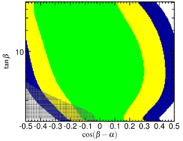
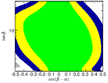
Figure 4: Direct constraints from LHC Higgs searches on the parameter space for the THDM Type I with $M_{\mathrm{H}}=300\,\mathrm{GeV}$ (left) and $M_{\mathrm{H}}=600\,\mathrm{GeV}$ (right). In both cases $M_{\mathrm{h}}=125\,\mathrm{GeV}$, $Z_{4}=Z_{5}=-2$ and $Z_{7}=0$ are given in the hybrid basis (c.f. Ref. [13]). The colours indicate compatibility with the observed Higgs signal at $1\,\sigma$ (green), $2\,\sigma$ (yellow), and $3\,\sigma$ (blue). Exclusion bounds at $95\%$ C.L. from the non-observation of the additional Higgs states are overlaid in gray. The graphics and description are taken from Ref. [13].

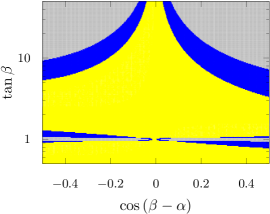
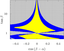
Figure 5: Example THDM parameter regions respecting perturbative unitarity and stability constraints (green) for the scenario of Fig. 6. The graphics are taken from Ref. [13].

Figure 6: The perturbativity measure for the scenario of Fig. 6. Gray areas are ruled out, while the blue and yellow areas show the maximal Higgs self-coupling strengths $\lambda/(4\pi)$ between 0.5 and 1, and 0.3 and 0.5, respectively. Parameter sets with values smaller than 0.3 do not occur.

Additionally, we employ perturbativity constraints to improve this scenario. Large coupling factors can lead to a breakdown of perturbation theory, so that we demand sufficiently small coupling factors. To this end, we compute the size of each coupling factor $\lambda(S_{1}S_{2}S_{3}S_{4})$ of all the four-point Higgs-boson vertices at tree level, where $S_{i}=h,H,A,G,H^{\pm},G^{\pm}$ for $i=1,\dots,4$, and use the largest coupling factor, $\lambda/(4\pi)=\max|\lambda(S_{1}S_{2}S_{3}S_{4})|/(4\pi)$, as a measure. We use Mathematica and our FeynArts model files exploiting the hybrid basis (c.f. Ref. [13]). The parameters $Z_{4}$, $Z_{5}$, and $Z_{7}$ of the hybrid basis are related to our input parameters via

$$M_{\mathrm{A_{0}}}^{2} =c_{\beta-\alpha}^{2}M_{\mathrm{h}}^{2}+M_{\mathrm{H}}^{2}s_{\beta-\alpha}^{2}-v^{2}Z_{5},$$ (3.5)

$$M_{\mathrm{H^{+}}}^{2} =M_{\mathrm{A_{0}}}^{2}-\frac{1}{2}v^{2}(Z_{4}-Z_{5}),$$ (3.6)

$$\lambda_{5} =Z_{5}+\frac{1}{2}t_{2\beta}\left[\frac{s_{2(\beta-\alpha)}}{2v^{2}}(M_{\mathrm{h}}^{2}-M_{\mathrm{H}}^{2})-Z_{7}\right]$$ (3.7)

with $v^{2}=1/(\sqrt{2}G_{\mu})$.

As the masses and mixing angles appear in the couplings, the perturbativity criterion gradually constrains the parameter space. Since the convergence of the perturbation series becomes worse with increasing coupling factors a clear discrimination of perturbative and non-perturbative parameter points is impossible. However, values of $\lambda/(4\pi)$ larger than $1$ indicate that higher-order corrections do not systematically become smaller and perturbativity is not given anymore which rules out such parameter points. Values between 0.5 and 1 usually still yield large higher-order corrections and need to be taken with care. The result of the perturbativity analysis is given in Fig. 6 for $M_{\mathrm{H}}=300\,\mathrm{GeV}$ (left) and $M_{\mathrm{H}}=600\,\mathrm{GeV}$ (right). Excluded areas are shown in gray, while blue ($0.5<\lambda/(4\pi)<1$) and yellow ($0.3<\lambda/(4\pi)<0.5$) indicate different sizes of the coupling factors. Parameter points where all couplings are smaller than 0.3 do not appear. The excluded trench at $\tan{\beta}=1$ is a singularity of the hybrid basis used in Ref. [13], since $t_{2\beta}$ in Eq. (3.7) and, hence, the coupling factors diverge at this point. Overlaying these results with the previous experimental and theoretical constraints shows a significant reduction of the allowed parameter region. Nevertheless, we need to modify the scenarios proposed by Ref. [13] only slightly to obtain the low- and high-mass scenarios as well as the benchmark plane scenario described later.

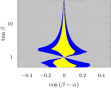
Figure 7: The perturbativity measure for $M_{\mathrm{H}}=1\,\mathrm{TeV}$ with the remaining parameters as in the scenario of Fig. 6. Large areas are excluded by coupling factors $\lambda/(4\pi)>1$ (gray) whereas values between 0.5 and 1 (0.3 and 0.5) are coloured blue (yellow).

We do not consider heavy Higgs masses in the TeV range, because the allowed parameter space is dramatically reduced in this region, which can be seen in Fig. 7. Only parameters close to the alignment limit and with $t_{\beta}\approx 2$ and $t_{\beta}\approx 0.5$ remain allowed for $|c_{\beta-\alpha}|\sim 0.1$.

1. Low-mass scenario: The low-mass scenario, which we already introduced in Ref. [40], consists of a heavy neutral CP-even Higgs boson ${\mathrm{H}}$ of mass $M_{\mathrm{H}}=300\,\mathrm{GeV}$. The input values are based on a benchmark scenario of Ref. [13] and consist of a THDM of Type I with

   $$M_{\mathrm{h}}=125\,\mathrm{GeV},\quad M_{\mathrm{H}}=300\,\mathrm{GeV},\quad M_{\mathrm{A_{0}}}=M_{\mathrm{H^{+}}}=460\,\mathrm{GeV},\quad\lambda_{5}=-1.9,\quad\tan\beta=2.$$ (3.8)

   Specifically, scenario A contains a scan in $c_{\beta-\alpha}$, as this is the only parameter of the THDM appearing at LO. The range of the scan is limited by constraints from experiments and perturbative unitarity. These constraints indicate that values of $|c_{\beta-\alpha}|$ exceeding 0.1 are phenomenologically disfavoured [13]. However, we perform our analysis with less stringent bounds to get a more complete picture. We take two distinguished points of the scan region named Aa and Ab with $c_{\beta-\alpha}=\pm 0.1$ to perform scale variations:

   $$\mbox{A:}\quad\cos{(\beta-\alpha)} =-0.2\ldots 0.2,$$ (3.9a)

   $$\mbox{Aa:}\quad\cos{(\beta-\alpha)} =+0.1,$$ (3.9b)

   $$\mbox{Ab:}\quad\cos{(\beta-\alpha)} =-0.1.$$ (3.9c)

2. High-mass scenario: The high-mass scenario is again based on a Type I THDM, however, with heavier Higgs bosons,

   $$M_{\mathrm{h}}=125\,\mathrm{GeV},\quad M_{\mathrm{H}}=600\,\mathrm{GeV},\quad M_{\mathrm{A_{0}}}=M_{\mathrm{H^{+}}}=690\,\mathrm{GeV}.$$ (3.10)

   Constraints from stability and perturbative unitarity (Fig. 6) reveal that positive and negative values of $c_{\beta-\alpha}$ are only allowed in different regions of $\tan{\beta}$. Therefore we define two parameter scans (B1, B2) which are applicable for positive (B1) and negative (B2) values of $c_{\beta-\alpha}$, and B1a, B2b are two distinguished points of the scan region:

   $$\mbox{B1:}\quad\cos{(\beta-\alpha)} =-0\ldots 0.15,\quad\lambda_{5}=-1.9,\quad\tan\beta=4.5,$$ (3.11a)

   $$\mbox{B1a:}\quad\cos{(\beta-\alpha)} =+0.1,$$ (3.11b)

   $$\mbox{B2:}\quad\cos{(\beta-\alpha)} =-0.15\ldots 0,\quad\lambda_{5}=-2.4,\quad\tan\beta=1.5,$$ (3.11c)

   $$\mbox{B2b:}\quad\cos{(\beta-\alpha)} =-0.1.$$ (3.11d)

3. Different THDM types: In this scenario, we compare different types of THDMs. Yukawa couplings appear in our process only in closed fermion loops in Higgs-boson two-point functions and in ${\mathrm{h}}VV$ and ${\mathrm{h}}gg$ vertex corrections, so that the top-quark contribution is dominant. The couplings to up-type quarks is identical in all types of THDM, so that we expect negligible effects from changing the type. The comparison is performed for scenarios Aa and B1a.

4. Benchmark plane: For this scenario, we analyze a large area of the $M_{\mathrm{H}}{-}\tan{\beta}$ plane:

   $$M_{\mathrm{H}} =300\ldots 750\,\mathrm{GeV},\quad\tan\beta=1\ldots 50.$$ (3.12)

   The fixed parameters are based on the Type I non-alignment scenario of Ref. [13], and are given in the hybrid basis (c.f. Ref. [13]) by

   $$\cos{(\beta-\alpha)} =0.1, M_{\mathrm{h}} =125\,\mathrm{GeV}, Z_{4} =Z_{5}=-2, Z_{7} =0.$$ (3.13)

5. Baryogenesis: The $\mathrm{BP3}_{B}$ scenario of Ref. [37] was initially proposed in Ref. [64]. With a second Higgs doublet, a first-order electroweak phase transition is possible, which could explain the baryon asymmetry in the universe. The main signature for this model is the decay of a pseudoscalar Higgs boson. Nevertheless, the non-alignment of the benchmark points $\mathrm{BP3}_{B}$ renders these scenarios also interesting for our study. The parameterization in the original form uses $m_{12}$ for the Higgs self-coupling parameter from which we compute $\lambda_{5}$ using

   $$m^{2}_{12} =c_{\beta}s_{\beta}(M_{\mathrm{A_{0}}}^{2}+\lambda_{5}v^{2}).$$ (3.14)

   The input parameters are

   $$M_{\mathrm{h}}=125\,\mathrm{GeV},\quad M_{\mathrm{H}}=200\,\mathrm{GeV},\quad M_{\mathrm{A_{0}}}=M_{\mathrm{H^{+}}}=420\,\mathrm{GeV},\quad\lambda_{5}=-2.58,\quad\tan\beta=3,$$

   and the two proposed scenarios differ by

   $$\mbox{$\mathrm{BP3}_{B1}$:}\quad\cos{(\beta-\alpha)} =0.3,\quad\text{Type I}$$ (3.15a)

   $$\mbox{$\mathrm{BP3}_{B2}$:}\quad\cos{(\beta-\alpha)} =0.5.\quad\text{Type II}$$ (3.15b)

6. Fermiophobic heavy Higgs: By choosing a Type I THDM as well as a vanishing mixing angle $\alpha$, the heavy Higgs boson ${\mathrm{H}}$ decouples from the fermions. Such a scenario was proposed in Ref. [10] with a direct detection of the heavy Higgs bosons as the leading signature. However, the alignment limit ($c_{\beta-\alpha}=0$) cannot be reached in this model as this would require large values of $\tan{\beta}$ which are ruled out by stability constraints. This gives rise to possibly sizable effects on the light Higgs-boson decay. Different $\tan{\beta}$ values can be chosen, and with larger values the alignment limit is approached:

   $$\mbox{$\mathrm{BP6}_{a}$:}\quad\tan{\beta} =40,$$ (3.16a)

   $$\mbox{$\mathrm{BP6}_{b}$:}\quad\tan{\beta} =20,$$ (3.16b)

   $$\mbox{$\mathrm{BP6}_{c}$:}\quad\tan{\beta} =10.$$ (3.16c)

   We transform the input parameter $m_{12}$ to our convention using Eq. (3.14) and use the same fixed $\lambda_{5}$ for all $\tan{\beta}$, and

   $$M_{\mathrm{h}}=125\,\mathrm{GeV},\quad M_{\mathrm{H}}=200\,\mathrm{GeV},\quad M_{\mathrm{A_{0}}}=M_{\mathrm{H^{+}}}=500\,\mathrm{GeV},\quad\lambda_{5}=-3.46\quad s_{\alpha}=0.$$ (3.17)

4 Numerical results

In this section we present our numerical results for the decay ${\mathrm{h}}\to 4f$ of the light CP-even Higgs boson ${\mathrm{h}}$ in the THDM for the different scenarios described in the previous section, beginning with the low-mass scenario. There, we investigate at first the conversion of the renormalized input parameters between different renormalization schemes and the running of the couplings. Afterwards we discuss the scale dependence of the $\mathrm{h}{\to}4f$ width and show the dependence on $c_{\beta-\alpha}$. First results of this study have already been published in Ref. [40]. Finally, we study the partial widths and differential distributions in order to identify deviations from the SM expectations. The same procedure is performed for the high-mass scenario (split into two regions with positive or negative $c_{\beta-\alpha}$), while we do not perform such a detailed analysis for the other scenarios.

4.1 Low-mass scenario

4.1.1 Conversion of the input parameters

The numerical values of an input parameter defined via different renormalization conditions in two renormalization schemes do in general not coincide in one and the same physics scenario, but have to be properly converted from one scheme to the other. This means that the mixing angles $\alpha$ and $\beta$ have to be converted in the transitions between the four renormalization schemes described in Sec. 2.2.2, as already discussed in Ref. [40]. For a generic parameter $p$, the renormalized values $p^{(1)}$ and $p^{(2)}$ in two different renormalization schemes 1 and 2 are connected via

$$p_{0}=p^{(1)}+\delta p^{(1)}(p^{(1)})=p^{(2)}+\delta p^{(2)}(p^{(2)}),$$ (4.1)

where $p_{0}$ is the corresponding bare parameter and $\delta p^{(1,2)}$ are the NLO renormalization constants of $\mathcal{O}(\alpha_{\mathrm{em}})$. In case of more parameters, this is a set of coupled equations. For the conversion of $p^{(2)}$ to $p^{(1)}$, we can either use the linearized solution

$$p^{(1)}=p^{(2)}+\delta p^{(2)}(p^{(2)})-\delta p^{(1)}(p^{(2)}),$$ (4.2)

where $\delta p^{(1)}(p^{(1)})$ is approximated by $\delta p^{(1)}(p^{(2)})$, or solve the set of implicit equations (4.1) numerically. The full solution of the implicit set of equations (4.1) has the advantage that converting parameters from one scheme to another and back is an identity, while this is only approximately the case in the linearized approach. The error of the linearized approximation is beyond our desired NLO accuracy as long as the perturbation series behaves well and higher-order terms are small. The comparison of the results obtained with the two methods allows for a consistency check of the computation. For the conversion of $\alpha$ and $\beta$, we employ the $\overline{\mathrm{MS}}$($\alpha$) scheme as one of the two schemes, so that we only have to deal with one set of finite counterterm contributions at a time.

In scenario A, we extend the range of $c_{\beta-\alpha}$ values to $-0.4$ to $0.4$, so that we get a larger picture even though the regions with large $|c_{\beta-\alpha}|$ are ruled out by phenomenology. The results are shown in Fig. 8 with a conversion from (l.h.s.) and to the $\overline{\mathrm{MS}}$$(\alpha)$ scheme (r.h.s.), while the $\overline{\mathrm{MS}}$$(\lambda_{3})$ (green), FJ($\alpha$) (pink), and FJ$(\lambda_{3})$ (turquoise) schemes are employed as the second scheme. All other conversions can be seen as a combination of the presented ones. On the left-hand side, the gray dashed lines are the result obtained using the linearized approximation. In both plots, we highlight the phenomenologically relevant region in the centre.

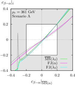
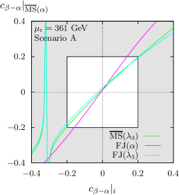
Figure 8: Panel (a): Conversion of the value of $c_{\beta-\alpha}$ from $\overline{\mathrm{MS}}$$(\alpha)$ to the $\overline{\mathrm{MS}}$$(\lambda_{3})$ (green), FJ($\alpha$) (pink), and FJ($\lambda_{3}$) schemes (turquoise) for scenario A. Panel (b) shows the conversion to the $\overline{\mathrm{MS}}$$(\alpha)$ scheme using the same colour coding. The solid lines are obtained by solving the implicit equations numerically, the dashed lines correspond to the linearized approximation. The phenomenologically relevant region is highlighted in the centre.

All curves show only small changes in the parameter values, and the numerical solution agrees well with the linearized conversion, affirming that the finite higher-order contributions of the counterterms are small, and perturbation theory is applicable. However, we would like to mention that a parameter set in the alignment limit $(c_{\beta-\alpha}\to 0)$ is not preserved in the conversion to other renormalization schemes. The alignment limit, thus, depends on the choice of the renormalization scheme. Outside the phenomenologically relevant region, the curves for the transformation involving the schemes with $\lambda_{3}$ as an independent parameter have a small region where large effects occur. This is an artifact as these schemes become singular at $c_{2\alpha}=0$. In the vicinity of the singularity (corresponding here to $c_{\beta-\alpha}\approx-0.32$), the $\overline{\mathrm{MS}}$ renormalization of $\lambda_{3}$ introduces large finite contributions to the conversion equation resulting in a breakdown of perturbation theory. This occurs in the $\overline{\mathrm{MS}}$$(\lambda_{3})$ and the FJ($\lambda_{3}$) renormalization schemes which limits their use. For scenario A, the phenomenologically relevant region is, however, not affected by this artifact.

4.1.2 The running of $c_{\beta-\alpha}$

Parameters renormalized in $\overline{\mathrm{MS}}$ depend on a renormalization scale $\mu_{\mathrm{r}}$, where the dependence is governed by the renormalization group equations (RGEs) of the THDM (see, e.g., Refs. [65, 66, 67, 68, 69]). For each renormalization scheme we solve the RGEs using a classical Runge–Kutta algorithm. We isolate the effects of the running from the conversion by considering each renormalization scheme separately, but do not convert the input values in this investigation. The scale dependence of $c_{\beta-\alpha}$ from $\mu_{\mathrm{r}}=100\,\mathrm{GeV}$ to $900\,\mathrm{GeV}$ is plotted in Fig. 9, for the scenarios Aa (l.h.s) and Ab (r.h.s) and input values given at the central scale $\mu_{0}$.

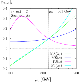
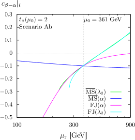
Figure 9: The running of $c_{\beta-\alpha}$ for scenarios Aa (a) and Ab (b) in the $\overline{\mathrm{MS}}$$(\alpha)$ (blue), $\overline{\mathrm{MS}}$$(\lambda_{3})$ (green), FJ($\alpha$) (pink), and FJ($\lambda_{3}$) (turquoise) schemes.

It shows that the choice of the renormalization scheme has a large impact on the scale dependence. While the $\overline{\mathrm{MS}}$$(\alpha)$ scheme introduces only a slow running, the other schemes show a much stronger scale dependence so that excluded and unphysical values of input parameters are reached quickly. A similar observation has also been made in supersymmetric models for the parameter $\tan\beta$ (the ratio of the vacuum expectation values of the Higgs doublets in SUSY models) in Ref. [42]: The gauge-dependent $\overline{\mathrm{MS}}$ schemes with vanishing renormalized tadpoles have a small scale dependence while replacing the parameters by gauge-independent ones introduces additional terms in the $\beta$-functions, which arrange for a stronger scale dependence of such schemes. We find similar results comparing the gauge-dependent $\overline{\mathrm{MS}}$ schemes with the gauge-independent FJ schemes in Fig. 9. It is remarkable that the sign of the slope differs for the different renormalization schemes. This is another consequence of the additional terms in the $\beta$-functions and shows that the choice of the renormalization scheme has large effects. As some curves hit the $c_{\beta-\alpha}=0$ axis and therefore run into the alignment limit, we explicitly see that this limit depends both on the renormalization scheme and on the renormalization scale in a given scheme. In Fig 9 one can also see that the curves for the $\overline{\mathrm{MS}}$$(\lambda_{3})$ and the FJ($\lambda_{3}$) scheme terminate around $250\,\mathrm{GeV}$. At this scale, the running of $\lambda_{3}$ yields unphysical values for the parameters of the theory. This is unique to the $\lambda_{3}$ running as only there an equation needs to be solved in the relation to $c_{\beta-\alpha}$. For the other cases we prevent the angles from running out of their domain of definition by solving the running for the tangent of the angles.

4.1.3 Scale variation of the width

Owing to the appearance of heavy Higgs bosons in the loop diagrams multiple scales occur in the calculation of the NLO EW corrections in the THDM. Therefore, a naive choice of the central renormalization scale of $\mu_{0}=M_{\mathrm{h}}$ might not be appropriate. To choose and to justify our central scale of Eq. (3.4), and to estimate the theoretical uncertainties, we compute the total width according to Eq. (2.1) while the scale is varied by roughly a factor of two around $\mu_{0}$. As a definition of the input parameters in each of the four renormalization schemes represents a physical scenario on its own, we have four input prescriptions ($\overline{\mathrm{MS}}$($\lambda_{3}$), $\overline{\mathrm{MS}}$$(\alpha)$, FJ($\alpha$), FJ($\lambda_{3}$)), and for each of them we compute the result in all renormalization schemes. After converting the input to the desired renormalization scheme, we evolve the $\overline{\mathrm{MS}}$ parameters from the scale $\mu_{0}$ to $\mu_{\mathrm{r}}$ by solving the RGEs, and finally compute the ${\mathrm{h}}{\to}4f$ width. The results are shown in Figs. 10 and 11 at LO (dashed) and NLO EW (solid) for the scenarios Aa and Ab for each of the input prescriptions.

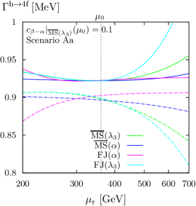
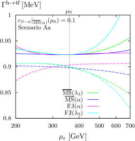
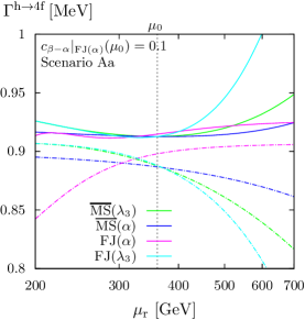
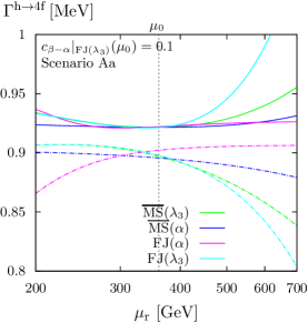
Figure 10: The ${\mathrm{h}}{\to}4f$ width at LO (dashed) and NLO EW (solid) for scenario Aa in dependence of the renormalization scale. The panels (a), (b), (c), and (d) correspond to input values defined in the $\overline{\mathrm{MS}}$$(\lambda_{3})$, $\overline{\mathrm{MS}}$$(\alpha)$, FJ($\alpha$), and FJ($\lambda_{3}$) schemes, respectively. The result is computed in all four different renormalization schemes after converting the input at NLO (also for the LO curves) and displayed using the colour code of Fig. 9.

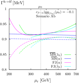
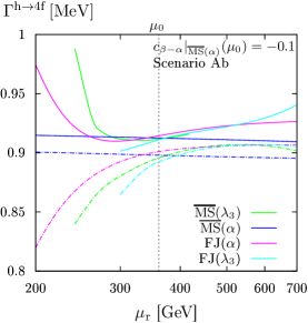
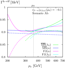
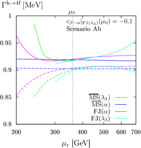
Figure 11: As in Fig. 10, but for scenario Ab.

The QCD corrections are not part of the EW scale variation and therefore omitted in these results.

The benchmark scenario Aa shows almost textbook-like behaviour, and the results are similar for all input prescriptions so that we discuss all of them simultaneously. First of all, the LO computation shows a strong scale dependence for all renormalization schemes, resulting in sizable differences between the curves. However, each of the NLO curves show a wide extremum with a large plateau, reducing the scale dependence drastically, as it is expected for NLO calculations. The central scale $\mu_{0}=(M_{\mathrm{h}}+M_{\mathrm{H}}+M_{\mathrm{A_{0}}}+2M_{\mathrm{H^{+}}})/5$ lies perfectly in the middle of the plateau regions justifying this scale choice. In contrast, the naive scale choice $\mu_{\mathrm{r}}=M_{\mathrm{h}}$ is not within the plateau region, leads to unnaturally large corrections, and should not be chosen. For all renormalization schemes, the plateaus coincide, and the agreement between the renormalization schemes is improved. This is expected since results obtained with different renormalization schemes should be equal up to higher-order terms, if the input parameters are properly converted. The relative renormalization scheme dependence at the central scale,

$$\Delta_{\mathrm{RS}}=2\,\frac{\Gamma^{{\mathrm{h}}{\to}4{\mathrm{f}}}_{\mathrm{max}}(\mu_{0})-\Gamma^{{\mathrm{h}}{\to}4{\mathrm{f}}}_{\mathrm{min}}(\mu_{0})}{\Gamma^{{\mathrm{h}}{\to}4{\mathrm{f}}}_{\mathrm{max}}(\mu_{0})+\Gamma^{{\mathrm{h}}{\to}4{\mathrm{f}}}_{\mathrm{min}}(\mu_{0})},$$ (4.3)

expresses the dependence of the result on the renormalization scheme. It can be computed for a specific input prescription from the difference of the smallest and largest width of the four renormalization schemes, $\Gamma^{{\mathrm{h}}{\to}4{\mathrm{f}}}_{\mathrm{min}}(\mu_{0})$ and $\Gamma^{{\mathrm{h}}{\to}4{\mathrm{f}}}_{\mathrm{max}}(\mu_{0})$, normalized to their average. In Tab. 3, $\Delta_{\mathrm{RS}}$ is given at LO and NLO for each of the input variants and confirms the reduction of the scheme dependence in the NLO calculation.

		$\overline{\mathrm{MS}}$$(\lambda_{3})$	$\overline{\mathrm{MS}}$$(\alpha)$	FJ($\alpha$)	FJ($\lambda_{3}$)
Scenario Aa:	$\Delta^{\mathrm{LO}}_{\mathrm{RS}}$[%]	0.67(0)	0.59(0)	1.25(0)	0.73(0)
	$\Delta^{\mathrm{NLO}}_{\mathrm{RS}}$ [%]	0.08(0)	0.06 (0)	0.27(0)	0.09(0)
Scenario Ab:	$\Delta^{\mathrm{LO}}_{\mathrm{RS}}$[%]	0.84(0)	1.00(0)	1.31(0)	0.63(0)
	$\Delta^{\mathrm{NLO}}_{\mathrm{RS}}$ [%]	0.34(0)	0.39(0)	0.49(1)	0.28(0)

Table 3: The variation $\Delta_{\mathrm{RS}}$ of the $\mathrm{h}{\to}4f$ width in scenarios Aa and Ab at the central scale $\mu_{0}$ using different renormalization schemes (with NLO parameter conversions). The columns correspond to the schemes in which the input parameters are defined. The technical uncertainty in brackets is calculated by exploiting the integration errors for the central values corresponding to the maximal and the minimal width.

In addition, the choice of the $\overline{\mathrm{MS}}$$(\alpha)$ scheme as an input scheme leads to the smallest dependence on the renormalization schemes in scenario Aa. This fits well to the observation perceived when the running was analyzed that the $\overline{\mathrm{MS}}$$(\alpha)$ scheme shows the smallest dependence on the renormalization scale, attesting a good absorption of further corrections into the NLO prediction.

The situation for benchmark scenario Ab is more subtle. For negative values of $c_{\beta-\alpha}$ the truncation of the schemes involving $\lambda_{3}$ at $\mu_{\mathrm{r}}=250{-}300\,\mathrm{GeV}$ as well as the breakdown of the running of the FJ($\alpha$) scheme, which both were observed in the running in Fig. 9, are also manifest in the computation of the ${\mathrm{h}}{\to}4f$ width. Therefore the results vary much more, and the extrema with the plateau regions are not as distinct as for the previous scenario, and even missing for some of the truncated curves. Nevertheless, the situation improves at NLO, and the relative renormalization scheme dependence reduces, as shown in Tab. 3. Also the central scale choice of $\mu_{0}$ seems to be appropriate in contrast to a naive choice of $M_{\mathrm{h}}$.

For both benchmark scenarios, the estimate of the theoretical uncertainties by varying the scale by a factor of two from the central value for an arbitrary renormalization scheme is generally not appropriate. A proper strategy would be to identify the renormalization schemes that yield reliable results, and to use only those to quantify the theoretical uncertainties from the scale variation. In addition, the renormalization scheme dependence of those schemes should be investigated. However, this procedure must be performed for each benchmark scenario separately, which is beyond the scope of this work for a larger list of benchmark scenarios.

4.1.4 $c_{\beta-\alpha}$ dependence

The dependence of the $\mathrm{h}{\to}4f$ width on $c_{\beta-\alpha}$ is one of the central results of our analysis, as the decay observables of the Higgs boson into four fermions in the THDM are most sensitive to this THDM parameter. The ${\mathrm{h}}{\to}4f$ width in dependence of $c_{\beta-\alpha}$ in scenario A is shown in Figs. 12–(d) for the four different input prescriptions.

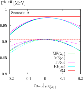
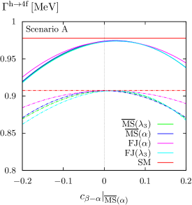
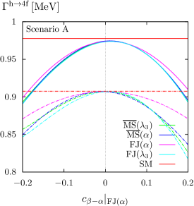
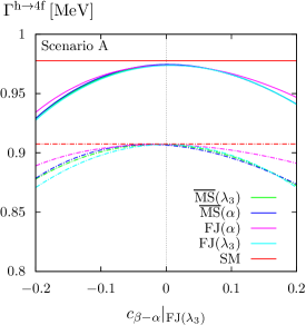
Figure 12: The $\mathrm{h}{\to}4f$ width at LO and full NLO EW+QCD (solid) for scenario A in dependence of $c_{\beta-\alpha}$. The panels (a), (b), (c), and (d) correspond to input values defined in the $\overline{\mathrm{MS}}$$(\lambda_{3})$, $\overline{\mathrm{MS}}$$(\alpha)$, FJ($\alpha$), and FJ($\lambda_{3}$) schemes, respectively. Parameters are consistently converted between the renormalization schemes (both for NLO and LO predictions) by numerically solving the non-linear matching equations (4.1). Results in the different target schemes are displayed with the colour code of Fig. 9, and the SM (with a SM Higgs-boson mass of $M_{\mathrm{h}}$) is shown for comparison in red.

The LO width with NLO conversion (dashed) and the full NLO EW+QCD total width (solid) are computed in the different renormalization schemes after the NLO input conversion, using the constant default scale $\mu_{0}$ of Eq. (3.4). The SM values with a SM Higgs-boson mass of $M_{\mathrm{h}}$ are illustrated in red. The results are similar for all input prescriptions so that we discuss them simultaneously. At LO they show the suppression w.r.t. to the SM with the factor $s_{\beta-\alpha}^{2}$. The differences at LO between the renormalization schemes are due to the conversion of the input. A pure LO computation is identical for all renormalization schemes, since there is no conversion in a pure LO prediction. This pure LO prediction is represented in each plot by the LO curve for which no conversion to another scheme is performed. The suppression w.r.t. to the SM computation does not change at NLO, while the shape becomes slightly asymmetric, and the NLO results show a significantly better agreement between the renormalization schemes. This is also confirmed by the relative renormalization scheme dependence shown in Fig. 13.

The relative corrections to the ${\mathrm{h}}{\to}4f$ width, defined by

$$\delta_{\mathrm{NLO}}=\delta_{\mathrm{QCD}}+\delta_{\mathrm{EW}}=\frac{\Gamma_{\mathrm{NLO}}}{\Gamma_{\mathrm{LO}}}-1,$$ (4.4)

are displayed in Fig. 14 for input parameters defined in the $\overline{\mathrm{MS}}$$(\lambda_{3})$ scheme.

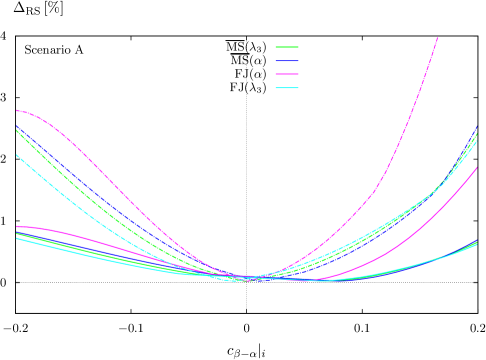
Figure 13: The relative dependence of the ${\mathrm{h}}{\to}4f$ width on the renormalization schemes as defined in Eq. (4.3) for the LO (dashed) and NLO EW+QCD (solid) calculation. The different colours correspond to calculations with input values defined in the different renormalization schemes, converted to the other schemes at NLO (converted parameters have also been used for the LO curves).

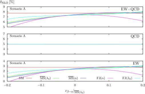
Figure 14: The relative NLO EW+QCD, QCD, and EW corrections to the ${\mathrm{h}}{\to}4f$ width in scenario A. The input values are defined in the $\overline{\mathrm{MS}}(\lambda_{3})$ scheme and converted to the other schemes at NLO (also for the LO curves). The results computed with different renormalization schemes are displayed with the colour code of Fig. 9.

For input parameters defined in the other schemes we obtain similar results, which are not shown. The different plots show the full EW+QCD ($\delta_{\mathrm{NLO}}$), the QCD ($\delta_{\mathrm{QCD}}$), and the EW corrections ($\delta_{\mathrm{EW}}$), where the first is just the sum of the two individual contributions. The relative QCD corrections lie practically on top of each other, so that only one line is visible even though the calculation was made in all renormalization schemes. The QCD corrections are almost identical to the SM case, which is not surprising as the interference of the diagram involving a closed quark loop (Fig. 3) is the only contribution in which the THDM amplitudes are not simple rescalings of their SM counterpart by the factor $s_{\beta-\alpha}$. Those diagrams contribute only little to the ${\mathrm{h}}{\to}4f$ width, so that the relative QCD corrections become similar to the SM. The EW corrections with the heavy Higgs bosons in the loop show a small asymmetry w.r.t. to the sign of $c_{\beta-\alpha}$ and are between 0 and $3\%$, even exceeding the relative corrections in the SM in the regions of large $c_{\beta-\alpha}$.

Deviations of the THDM results from the SM can be investigated when the SM Higgs-boson mass is identified with the mass of the light Higgs boson ${\mathrm{h}}$ of the THDM. The relative deviation of the full width from the SM is then

$$\Delta_{\mathrm{SM}}=\frac{\Gamma_{\mathrm{THDM}}-\Gamma_{\mathrm{SM}}}{\Gamma_{\mathrm{SM}}},$$ (4.5)

which is shown in Fig. 15 at LO (dashed) and NLO (solid) for parameters defined in the $\overline{\mathrm{MS}}$$(\lambda_{3})$ scheme (other input definitions yield similar results).

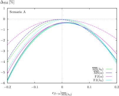
Figure 15: The relative difference of the ${\mathrm{h}}{\to}4f$ decay width in the THDM w.r.t. the SM prediction at LO (dashed) and NLO EW+QCD (solid). The input scheme is $\overline{\mathrm{MS}}$$(\lambda_{3})$, and the corrections are computed in all four renormalization schemes after converting the input at NLO (also for the LO curves), which are displayed using the colour code of Fig. 9.

The SM exceeds the THDM widths at LO and NLO. At LO the shape of $c_{\beta-\alpha}^{2}$ can be seen, with modifications due to input conversion. This shape is slightly distorted at NLO by the asymmetry of the EW corrections, and a small offset of $-0.5$% is visible even in the alignment limit where the diagrams including heavy Higgs bosons still contribute. The NLO computations show larger negative deviations, which could be used to improve current exclusion bounds or increase their significance. Nevertheless, in the whole scan region the deviation from the SM is within $6\%$ and for the parameter region with $|c_{\beta-\alpha}|<0.1$ even less than $2\%$, which will be challenging for experiments to measure.

We also investigate the origin of the relative EW corrections. To this end, in Fig. 16 we plot different contributions to the full correction in the $\overline{\mathrm{MS}}$($\lambda_{3}$) renormalization scheme (the breakup in the other schemes is qualitatively similar).

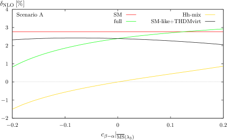
Figure 16: The full relative NLO corrections to ${\mathrm{h}}{\to}4f$ (green) split into different subcontributions. The SM-like contribution consists of all diagrams that have a SM equivalent, the THDM-virt contribution includes all one-loop and counterterm contributions that involve heavy Higgs bosons (sum of the two parts shown in black), and Hh-mixing contribution is displayed in yellow. For comparison, the relative NLO corrections in the SM are shown in red.

The contribution called “SM-like+THDM-virt” comprises all diagrams that have a SM correspondence as well as the real corrections of Eq. (2.10), and the diagrams of Fig. 2 with at least one heavy Higgs boson in the loop and the contributions of heavy Higgs bosons to the counterterms. The part called “Hh-mix” is defined by the contributions of the Hh-mixing field renormalization constant $\delta Z_{{\mathrm{H}}{\mathrm{h}}}$ and the renormalization constant $\delta\alpha$ in Eq. (2.9). Note that this splitting is neither gauge-independent, nor UV-finite. However, the major contribution to the Hh-mix part is furnished by Higgs-boson loops, which do not depend on the gauge, so that some qualitative conclusions may be drawn. The SM-like+THDM-virt diagrams shows a small off-set from the SM result and only a small $c_{\beta-\alpha}$ dependence, showing that the modification of the coupling factors in the THDM is small, but grows when the alignment limit is left. In the alignment limit, the off-set originates only from the heavy Higgs boson contribution, since only these diagrams introduce differences w.r.t. the SM. For values of $|c_{\beta-\alpha}|>0.05$ the major deviation from the SM and the shape of the EW corrections are mainly due to the Hh Higgs mixing. These terms factorize from the LO contribution and thus lead to a uniform (i.e. phase-space independent) and universal (i.e. final-state independent) correction factor to the LO prediction.

4.1.5 Partial widths for individual four-fermion states

The partial ${\mathrm{h}}{\to}4f$ widths (as defined in Sec. 2) at NLO are shown in the $\overline{\mathrm{MS}}$$(\lambda_{3})$ scheme for benchmark scenarios Aa and Ab in Tabs. 5 and 5, respectively.

$\Big{|}$ Final state	$\Gamma^{{\mathrm{h}}{\to}4f}_{\mathrm{NLO}}$ [MeV]	$\delta_{\mathrm{EW}}$ [%]	$\delta_{\mathrm{QCD}}$ [%]	$\Delta_{\mathrm{SM}}^{\mathrm{NLO}}$ [%]	$\Delta_{\mathrm{SM}}^{\mathrm{LO}}$ [%]
inclusive ${\mathrm{h}}{\to}4f$	$0.96730(7)$	$2.71(0)$	$4.96(1)$	$-1.05(1)$	$-1.00(1)$
ZZ	$0.106126(6)$	$0.34(0)$	$4.88(0)$	$-1.13(1)$	$-1.00(0)$
WW	$0.86630(8)$	$3.00(0)$	$5.01(1)$	$-1.04(1)$	$-1.00(1)$
WW/ZZ int.	$-0.00513(5)$	$1.3(2)$	$12.0(8)$	$-1(1)$	$-1(1)$
$\nu_{\mathrm{e}}{\mathrm{e}}^{+}\mu^{-}\bar{\nu}_{\mu}$	$0.010201(1)$	$3.03(0)$	$0.00$	$-1.04(1)$	$-1.00(1)$
$\nu_{\mathrm{e}}{\mathrm{e}}^{+}{\mathrm{u}}\bar{{\mathrm{d}}}$	$0.031719(4)$	$3.02(0)$	$3.76(1)$	$-1.04(2)$	$-1.00(1)$
${\mathrm{u}}\bar{{\mathrm{d}}}{\mathrm{s}}\bar{{\mathrm{c}}}$	$0.09847(2)$	$2.97(0)$	$7.52(1)$	$-1.04(2)$	$-1.00(1)$
$\nu_{\mathrm{e}}{\mathrm{e}}^{+}{\mathrm{e}}^{-}\bar{\nu}_{\mathrm{e}}$	$0.010197(1)$	$3.12(0)$	$0.00$	$-1.04(1)$	$-1.00(1)$
${\mathrm{u}}\bar{{\mathrm{d}}}{\mathrm{d}}\bar{{\mathrm{u}}}$	$0.10048(2)$	$2.85(0)$	$7.35(2)$	$-1.06(3)$	$-1.00(1)$
$\nu_{\mathrm{e}}\bar{\nu}_{\mathrm{e}}\nu_{\mu}\bar{\nu}_{\mu}$	$0.000949(0)$	$3.01(0)$	$0.00$	$-1.14(1)$	$-1.00(1)$
${\mathrm{e}}^{-}{\mathrm{e}}^{+}\mu^{-}\mu^{+}$	$0.000239(0)$	$1.30(1)$	$0.00$	$-1.13(2)$	$-1.00(1)$
$\nu_{\mathrm{e}}\bar{\nu}_{\mathrm{e}}\mu^{-}\mu^{+}$	$0.000477(0)$	$2.45(1)$	$0.00$	$-1.13(2)$	$-1.00(1)$
$\nu_{\mathrm{e}}\bar{\nu}_{\mathrm{e}}\nu_{\mathrm{e}}\bar{\nu}_{\mathrm{e}}$	$0.000569(0)$	$2.90(0)$	$0.00$	$-1.14(2)$	$-1.00(1)$
${\mathrm{e}}^{-}{\mathrm{e}}^{+}{\mathrm{e}}^{-}{\mathrm{e}}^{+}$	$0.000132(0)$	$1.12(1)$	$0.00$	$-1.12(2)$	$-1.00(1)$
$\nu_{\mathrm{e}}\bar{\nu}_{\mathrm{e}}{\mathrm{u}}\bar{{\mathrm{u}}}$	$0.001679(0)$	$0.60(1)$	$3.76(1)$	$-1.12(2)$	$-1.00(1)$
$\nu_{\mathrm{e}}\bar{\nu}_{\mathrm{e}}{\mathrm{d}}\bar{{\mathrm{d}}}$	$0.002177(1)$	$1.69(0)$	$3.76(1)$	$-1.12(2)$	$-1.00(1)$
${\mathrm{e}}^{-}{\mathrm{e}}^{+}{\mathrm{u}}\bar{{\mathrm{u}}}$	$0.000845(0)$	$0.11(1)$	$3.76(1)$	$-1.12(2)$	$-1.00(1)$
${\mathrm{e}}^{-}{\mathrm{e}}^{+}{\mathrm{d}}\bar{{\mathrm{d}}}$	$0.001088(0)$	$0.47(1)$	$3.76(1)$	$-1.12(2)$	$-1.00(1)$
${\mathrm{u}}\bar{{\mathrm{u}}}{\mathrm{c}}\bar{{\mathrm{c}}}$	$0.002971(0)$	$-1.80(1)$	$7.51(1)$	$-1.11(2)$	$-1.00(1)$
${\mathrm{d}}\bar{{\mathrm{d}}}{\mathrm{d}}\bar{{\mathrm{d}}}$	$0.002556(1)$	$-0.38(0)$	$4.38(2)$	$-1.21(3)$	$-1.00(1)$
${\mathrm{d}}\bar{{\mathrm{d}}}{\mathrm{s}}\bar{{\mathrm{s}}}$	$0.004956(1)$	$-0.36(0)$	$7.51(1)$	$-1.12(2)$	$-1.00(1)$
${\mathrm{u}}\bar{{\mathrm{u}}}{\mathrm{s}}\bar{{\mathrm{s}}}$	$0.003852(1)$	$-0.66(1)$	$7.51(1)$	$-1.11(2)$	$-1.00(1)$
${\mathrm{u}}\bar{{\mathrm{u}}}{\mathrm{u}}\bar{{\mathrm{u}}}$	$0.001506(0)$	$-1.92(1)$	$4.06(3)$	$-1.24(4)$	$-1.00(1)$

Table 4: Partial widths for benchmark scenario Aa in the $\overline{\mathrm{MS}}$$(\lambda_{3})$ renormalization scheme.

$\Big{|}$ Final state	$\Gamma^{{\mathrm{h}}{\to}4f}_{\mathrm{NLO}}$ [MeV]	$\delta_{\mathrm{EW}}$ [%]	$\delta_{\mathrm{QCD}}$ [%]	$\Delta_{\mathrm{SM}}^{\mathrm{NLO}}$ [%]	$\Delta_{\mathrm{SM}}^{\mathrm{LO}}$ [%]
inclusive ${\mathrm{h}}{\to}4f$	$0.95980(7)$	$1.87(0)$	$4.97(1)$	$-1.82(1)$	$-1.00(1)$
ZZ	$0.105464(5)$	$-0.34(0)$	$4.90(0)$	$-1.75(1)$	$-1.00(0)$
WW	$0.85938(8)$	$2.14(0)$	$5.01(1)$	$-1.83(1)$	$-1.00(1)$
WW/ZZ int.	$-0.00504(5)$	$0.5(1)$	$10.7(8)$	$-2(1)$	$-1(1)$
$\nu_{\mathrm{e}}{\mathrm{e}}^{+}\mu^{-}\bar{\nu}_{\mu}$	$0.010116(1)$	$2.17(1)$	$0.00$	$-1.87(1)$	$-1.00(1)$
$\nu_{\mathrm{e}}{\mathrm{e}}^{+}{\mathrm{u}}\bar{{\mathrm{d}}}$	$0.031463(4)$	$2.16(0)$	$3.76(1)$	$-1.84(2)$	$-1.00(1)$
${\mathrm{u}}\bar{{\mathrm{d}}}{\mathrm{s}}\bar{{\mathrm{c}}}$	$0.09770(2)$	$2.11(0)$	$7.52(1)$	$-1.81(2)$	$-1.00(1)$
$\nu_{\mathrm{e}}{\mathrm{e}}^{+}{\mathrm{e}}^{-}\bar{\nu}_{\mathrm{e}}$	$0.010112(1)$	$2.27(1)$	$0.00$	$-1.87(1)$	$-1.00(1)$
${\mathrm{u}}\bar{{\mathrm{d}}}{\mathrm{d}}\bar{{\mathrm{u}}}$	$0.09972(2)$	$1.99(0)$	$7.38(2)$	$-1.80(2)$	$-1.00(1)$
$\nu_{\mathrm{e}}\bar{\nu}_{\mathrm{e}}\nu_{\mu}\bar{\nu}_{\mu}$	$0.000943(0)$	$2.34(0)$	$0.00$	$-1.78(1)$	$-1.00(1)$
${\mathrm{e}}^{-}{\mathrm{e}}^{+}\mu^{-}\mu^{+}$	$0.000237(0)$	$0.62(1)$	$0.00$	$-1.79(2)$	$-1.00(1)$
$\nu_{\mathrm{e}}\bar{\nu}_{\mathrm{e}}\mu^{-}\mu^{+}$	$0.000474(0)$	$1.78(1)$	$0.00$	$-1.78(2)$	$-1.00(1)$
$\nu_{\mathrm{e}}\bar{\nu}_{\mathrm{e}}\nu_{\mathrm{e}}\bar{\nu}_{\mathrm{e}}$	$0.000565(0)$	$2.23(0)$	$0.00$	$-1.79(2)$	$-1.00(1)$
${\mathrm{e}}^{-}{\mathrm{e}}^{+}{\mathrm{e}}^{-}{\mathrm{e}}^{+}$	$0.000131(0)$	$0.45(1)$	$0.00$	$-1.78(2)$	$-1.00(1)$
$\nu_{\mathrm{e}}\bar{\nu}_{\mathrm{e}}{\mathrm{u}}\bar{{\mathrm{u}}}$	$0.001668(0)$	$-0.08(1)$	$3.76(1)$	$-1.76(2)$	$-1.00(1)$
$\nu_{\mathrm{e}}\bar{\nu}_{\mathrm{e}}{\mathrm{d}}\bar{{\mathrm{d}}}$	$0.002163(0)$	$1.02(0)$	$3.76(1)$	$-1.76(2)$	$-1.00(1)$
${\mathrm{e}}^{-}{\mathrm{e}}^{+}{\mathrm{u}}\bar{{\mathrm{u}}}$	$0.000840(0)$	$-0.57(1)$	$3.76(1)$	$-1.77(2)$	$-1.00(1)$
${\mathrm{e}}^{-}{\mathrm{e}}^{+}{\mathrm{d}}\bar{{\mathrm{d}}}$	$0.001081(0)$	$-0.21(1)$	$3.76(1)$	$-1.76(2)$	$-1.00(1)$
${\mathrm{u}}\bar{{\mathrm{u}}}{\mathrm{c}}\bar{{\mathrm{c}}}$	$0.002952(0)$	$-2.48(1)$	$7.51(1)$	$-1.75(2)$	$-1.00(1)$
${\mathrm{d}}\bar{{\mathrm{d}}}{\mathrm{d}}\bar{{\mathrm{d}}}$	$0.002545(1)$	$-1.06(0)$	$4.57(2)$	$-1.67(3)$	$-1.00(1)$
${\mathrm{d}}\bar{{\mathrm{d}}}{\mathrm{s}}\bar{{\mathrm{s}}}$	$0.004925(1)$	$-1.04(0)$	$7.51(1)$	$-1.74(2)$	$-1.00(1)$
${\mathrm{u}}\bar{{\mathrm{u}}}{\mathrm{s}}\bar{{\mathrm{s}}}$	$0.003828(1)$	$-1.35(1)$	$7.51(1)$	$-1.74(2)$	$-1.00(1)$
${\mathrm{u}}\bar{{\mathrm{u}}}{\mathrm{u}}\bar{{\mathrm{u}}}$	$0.001500(0)$	$-2.60(1)$	$4.31(2)$	$-1.65(3)$	$-1.00(1)$

Table 5: Partial widths for benchmark scenario Ab in the $\overline{\mathrm{MS}}$$(\lambda_{3})$ renormalization scheme.

For other schemes, the numbers differ slightly, but show the same qualitative pattern, so that we do not show them here. In the tables, we do not only state the full NLO QCD+EW partial widths, but also the relative EW and QCD corrections. The qualitative picture is similar for the two benchmark scenarios. The WW contribution originating from charged-current final states yields the largest contribution, while the ZZ contribution is minor and the interference term yields a small negative contribution. The EW corrections to the WW-mediated final states are uniformly about $2{-}3$%, which determine the EW corrections to the partial ${\mathrm{h}}{\to}4f$ width. The EW corrections to the neutral-current final states strongly depend on the fermion flavour and range between $\pm 3\%$. The QCD corrections are essentially the strong corrections to ${\mathrm{W}}/{\mathrm{Z}}\to q\bar{q}$ and therefore amount to $\alpha_{\mathrm{s}}/\pi$ for each pair of quarks in the final state. The ${\mathrm{u}}\bar{{\mathrm{u}}}{\mathrm{u}}\bar{{\mathrm{u}}}$ and ${\mathrm{d}}\bar{{\mathrm{d}}}{\mathrm{d}}\bar{{\mathrm{d}}}$ final states, where interference contributions between two different ZZ channels exist, are somewhat exceptional with QCD corrections of only about $4\%$. The deviations $\Delta_{\mathrm{SM}}$ from the SM expectation are shown at NLO and LO in the last two columns. The LO deviation is due to the suppression factor $s_{\beta-\alpha}$ of the ${\mathrm{h}}VV$ coupling w.r.t. the SM and therefore identical with $s_{\beta-\alpha}^{2}-1=-c_{\beta-\alpha}^{2}=-10^{-2}$ for all final states, since $c_{\beta-\alpha}=\pm 0.1$. It should be noted that the indicated errors are integration errors, and the presented LO results are thus also a consistency check. At NLO the deviation is slightly larger, though still within only 1.3% (2%) for the Aa (Ab) benchmark scenario. The deviations from the SM are quite uniform, i.e. insensitive to the final state, so that they are described by the partial ${\mathrm{h}}{\to}4f$ width well within a few per mille.

4.1.6 Differential distributions

The program Prophecy4f provides invariant-mass and angular differential distributions for the ${\mathrm{h}}{\to}4f$ decays. The differential decay widths may serve as a window to observe BSM effects as the shape of distributions might be distorted significantly by new coupling structures. This might occur even if the partial widths do not change significantly, and therefore, the differential distributions of leptonic and semi-leptonic final states (see Sec. 2) are important observables. In the following, we study them for both charged- and neutral-current processes, e.g. the fully leptonic final states ${\mathrm{e}}^{-}{\mathrm{e}}^{+}\mu^{-}\mu^{+}$ (nc), $\nu_{\mathrm{e}}{\mathrm{e}}^{+}\mu^{-}\bar{\nu}_{\mu}$ (cc), and the semi-leptonic final states ${\mathrm{e}}^{-}{\mathrm{e}}^{+}q\bar{q}$ (nc), $\nu_{\mathrm{e}}{\mathrm{e}}^{+}{\mathrm{d}}\bar{{\mathrm{u}}}$ (cc). Most likely, differential distributions for fully hadronic final states are not experimentally accessible. A detailed discussion of the SM distributions at NLO, including issues of final-state radiation (such as photon recombination), can be found for the fully leptonic final states in Refs. [30, 31, 36] and for semi-leptonic final states in Ref. [32]. In our study we emphasize the differences between the SM and the THDM results, while the features of photonic (and gluonic) corrections in the THDM and the SM are identical. The distributions discussed in the following are calculated using the $\overline{\mathrm{MS}}$$(\lambda_{3})$ renormalization scheme; the other renormalization schemes yield similar results.

Leptonic final states:

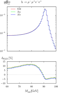
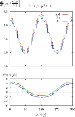
Figure 17: Invariant-mass (a) and angular distributions (b) of the leptonic neutral-current decay $\mathrm{h}\to\mu^{-}\mu^{+}{\mathrm{e}}^{-}{\mathrm{e}}^{+}$ for the SM and the THDM benchmark scenarios Aa and Ab. The relative NLO corrections to the distributions are plotted in the lower panels.

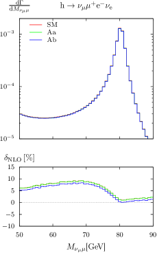
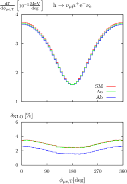
Figure 18: As in Fig. 18, but for the leptonic charged-current decay $\mathrm{h}\to\nu_{\mu}\mu^{+}{\mathrm{e}}^{-}\bar{\nu}_{\mathrm{e}}$.

We begin with the leptonic final state ${\mathrm{e}}^{-}{\mathrm{e}}^{+}\mu^{-}\mu^{+}$ which is a decay mediated by Z bosons. The invariant mass $M_{f_{a}\bar{f}_{b}}$ of a fermion–anti-fermion pair is defined by

$$M^{2}_{f_{a}\bar{f}_{b}}=(k_{a}+k_{b})^{2}$$ (4.6)

with the momentum $k_{a}$ of the fermion $f_{a}$ and $k_{b}$ of the anti-fermion $\bar{f}_{b}$, where the photon momentum is already added to the fermion momentum in case of recombination. The NLO invariant-mass distributions of the muon pair are displayed in the first panel of Fig. 18 for the SM and the THDM in scenarios Aa and Ab and show the Z-boson resonance. The relative corrections normalized to the LO are illustrated in the second panel and exhibit the well-known effects of final-state radiation near the Z resonance: Photons radiated off a final-state lepton lower the invariant mass of the lepton pair and lead to positive corrections—the “radiative tail”—for invariant masses below the Z-boson peak and negative corrections above. These corrections would contain a logarithm of the form $\alpha\ln(m_{\mu}/M_{\mathrm{h}})$ from collinear photon emission off muons if no photon recombination was applied. However, photon recombination mitigates this large effect by shifting events back to larger invariant masses for collinear emission and leads to the necessary level of inclusiveness required by the Kinoshita–Lee–Nauenberg theorem [70, 71] to remove the collinear singularity. In case of photon recombination, the $\mu^{-}\mu^{+}$ and ${\mathrm{e^{-}}}{\mathrm{e^{+}}}$ invariant-mass distributions are, thus, identical. Yet, non-collinear photons, which are not recombined, still lead to a sizable net effect which is observed in the relative corrections. The shapes of the invariant-mass distributions in SM and THDM are practically identical, i.e. the impact of new Lorentz structures in the NLO THDM diagrams is negligible. The relative difference between the SM and the THDM distributions is just given by the difference observed already in the integrated ${\mathrm{h}}{\to}{\mathrm{e}}^{-}{\mathrm{e}}^{+}\mu^{-}\mu^{+}$ decay width, i.e. $-1.15$% for scenario Aa and $-1.81$% for Ab. We recall that those differences were traced back to the impact of ${\mathrm{H}}{\mathrm{h}}$-mixing effects in Sec. 4.1.4, which are independent from the decay kinematics, and thus conclude that those mixing effects are the dominant higher-order effects visible in the distributions as well.

The differential decay width with respect to the angle $\phi$ between the $\mu^{-}\mu^{+}$ and ${\mathrm{e}}^{-}{\mathrm{e}}^{+}$ decay planes is defined by

$$\cos\phi=\frac{\left(\left(\mathbf{k}_{1}+\mathbf{k}_{2}\right)\times\mathbf{k}_{1}\right)\cdot((\mathbf{k}_{1}+\mathbf{k}_{2})\times\mathbf{k}_{3})}{|(\mathbf{k}_{1}+\mathbf{k}_{2})\times\mathbf{k}_{1}||(\mathbf{k}_{1}+\mathbf{k}_{2})\times\mathbf{k}_{3}|},$$ (4.7)

with the sign convention

$$\mathrm{sgn}(\sin\phi)=\mathrm{sgn}\{\left(\mathbf{k}_{1}+\mathbf{k}_{2}\right)\cdot\left[\left(\left(\mathbf{k}_{1}+\mathbf{k}_{2}\right)\times\mathbf{k}_{1}\right)\times\left(\left(\mathbf{k}_{1}+\mathbf{k}_{2}\right)\times\mathbf{k}_{3}\right)\right]\}$$ (4.8)

where $\mathbf{k}_{1}$, $\mathbf{k}_{2}$, and $\mathbf{k}_{3}$ are the momenta of the muon, the anti-muon and the electron, respectively. The corresponding distribution is shown in the upper panel of Fig. 18. One observes a $\cos{(2\phi)}$ pattern in the shape of the distribution, which can be used to set bounds on non-standard couplings of the Higgs boson to the EW gauge bosons (see Refs. [22, 23, 24, 25, 26, 27, 28, 29]). Note that the oscillation pattern in the distribution of a pseudo-scalar Higgs boson would have a different sign. We again observe that the SM shape is not distorted by THDM effects and that the difference between SM and THDM prediction just resembles the difference in the integrated widths.

We have also considered the invariant-mass and angular distributions of the ${\mathrm{e}}^{-}{\mathrm{e}}^{+}{\mathrm{e}}^{-}{\mathrm{e}}^{+}$ final state (not shown), for which interference terms between different ZZ channels appear. There, the assignment of the lepton pairs to intermediate Z bosons is not unique; usually the electron and positron with an invariant mass closest to the Z-boson mass is combined to a pair. Again we find that the relative difference $\Delta_{\mathrm{SM}}$ between THDM and the SM is practically constant over the phase space and given by its values for the integrated width.

For the W-boson-mediated $\nu_{\mathrm{e}}{\mathrm{e}}^{+}\mu^{-}\bar{\nu}_{\mu}$ final state, the respective distributions are shown in Fig. 18. The invariant-mass distribution of $M_{\nu_{\mu}{\mu}}$ is not experimentally accessible, but shown for theoretical interest. The plot shows the W resonance around $M_{\nu_{\mu}\mu}\approx M_{\mathrm{W}}$ with the radiative corrections caused by photon radiation as discussed above. As already observed in the neutral-current final state, there is no significant shape distortion in the THDM w.r.t. the SM prediction. As the neutrinos cannot be detected, neither the Higgs nor the W boson can be fully reconstructed. However, projecting all lepton momenta into a fixed plane mimics the experimental situation at the LHC in the centre-of-mass frame of the Higgs boson in the plane transverse to the proton beams, where the sum of the neutrino momenta is measurable as missing momentum. We, thus, analyze the transverse angle $\phi_{\mu{\mathrm{e}},{\mathrm{T}}}$ between the two charged leptons [30], defined by

$$\cos\phi_{\mu{\mathrm{e}},{\mathrm{T}}} =\frac{\mathbf{k}_{\mu,{\mathrm{T}}}\cdot\mathbf{k}_{{\mathrm{e}},{\mathrm{T}}}}{|\mathbf{k}_{\mu,{\mathrm{T}}}||\mathbf{k}_{{\mathrm{e}},{\mathrm{T}}}|}, \mathrm{sgn}(\sin\phi_{\mathrm{T}}) =\mathrm{sgn}\{\mathbf{e}_{z}\cdot(\mathbf{k}_{\mu,{\mathrm{T}}}\times\mathbf{k}_{{\mathrm{e}},{\mathrm{T}}})\},$$ (4.9)

where $\mathbf{k}_{i,{\mathrm{T}}}$ are the parts of the full lepton momenta $\mathbf{k}_{i}$ orthogonal to the fixed unit vector $\mathbf{e}_{z}$ representing the beam direction of the Higgs-boson production process. The distribution in $\phi_{\mu{\mathrm{e}},{\mathrm{T}}}$ is shown in the first panel of Fig. 18. As expected, no shape distortion is seen w.r.t. the SM prediction, only the constant relative deviation which is identical to the deviation in the partial width of $-1.04$% (Aa) and $-1.87$% (Ab). Other fully leptonic final states show similar patterns, so that their distributions are not separately shown here.

Semi-leptonic final states:

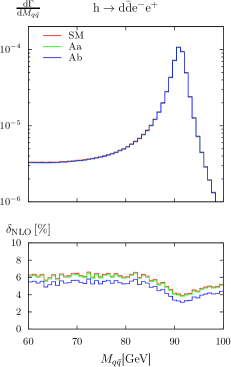
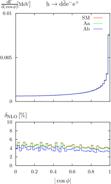
Figure 19: Invariant-mass (a) and angular distributions (b) of the charged-current semi-leptonic decay $\mathrm{h}\to{\mathrm{d}}\bar{{\mathrm{d}}}{\mathrm{e}}^{-}{\mathrm{e}}^{+}$ for the SM and the THDM benchmark scenarios Aa and Ab. The relative NLO EW+QCD corrections to the distributions are plotted in the lower panels.

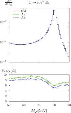
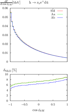
Figure 20: As for Fig. 20, but for the charged-current semi-leptonic decay $\mathrm{h}\to\nu_{\mathrm{e}}{\mathrm{e}}^{+}{\mathrm{d}}\bar{{\mathrm{u}}}$.

The invariant-mass distribution of the hadronic system of the neutral-current final state ${\mathrm{d}}\bar{{\mathrm{d}}}{\mathrm{e}}^{-}{\mathrm{e}}^{+}$ is displayed in Fig. 20 (l.h.s), together with the corresponding NLO EW+QCD corrections. In case of gluon radiation, the invariant mass is built from the whole hadronic $q\bar{q}g$ system to obtain an IR-safe observable. The distribution and the corrections show similar characteristics to the ones of the corresponding leptonic final state: Photon radiation leads to a radiative tail, but SM and THDM distributions do not show any visible shape difference. Note that the effect of the photon radiation is less pronounced compared to the leptonic final state, as the quark charge factors are smaller than for leptons. There is no radiative tail from gluon radiation, because all gluons are recombined with the quark pair, so that only a flat QCD correction remains [32].

In order to analyze angular distributions, we identify the quarks and antiquarks with jets for events without gluon radiation. In case of gluon radiation, we always combine the two QCD partons with the smallest invariant mass to a single jet, so that we again obtain an event with two jets. As the jets cannot be distinguished, any observable must be invariant under the permutation of the two jets. For this reason, the angle $\phi$ between the two Z-boson decay planes can only be reconstructed up to the sign of $\cos\phi$, so that we define [32]

$$|\cos\phi|=\left|\frac{\left(\left(\mathbf{k}_{\mathrm{jet}_{1}}+\mathbf{k}_{\mathrm{jet}_{2}}\right)\times\mathbf{k}_{{\mathrm{e^{-}}}}\right)\left(\mathbf{k}_{\mathrm{jet}_{1}}\times\mathbf{k}_{\mathrm{jet}_{2}}\right)}{|\left(\mathbf{k}_{\mathrm{jet}_{1}}+\mathbf{k}_{\mathrm{jet}_{2}}\right)\times\mathbf{k}_{{\mathrm{e^{-}}}}||\mathbf{k}_{\mathrm{jet}_{1}}\times\mathbf{k}_{\mathrm{jet}_{2}}|}\right|.$$ (4.10)

The corresponding distribution, which is depicted on the r.h.s. of Fig. 20, looks rather different from the leptonic case, since $|\cos\phi|$ instead of $\phi$ is used in the binning. Again, the major finding is the fact that the shape of the distribution does not change in the transition from the SM to the THDM. Only the flat offsets of $-1.12$% (Aa) and $-1.76$% (Ab) already encountered in the partial width are visible.

The invariant-mass distribution of the hadronic system of the semi-leptonic W-boson-mediated final state $\nu_{\mathrm{e}}{\mathrm{e}}^{+}{\mathrm{d}}\bar{{\mathrm{u}}}$ is pictured in Fig. 20 (l.h.s) and shows the same characteristics as the one of the neutral-current final state considered above: a moderate radiative tail from photon radiation, flat QCD corrections (not explicitly shown), and no shape difference between SM and THDM predictions. The distribution in the angle between the electron and the hadronically decaying W boson, $\phi_{{\mathrm{e}}{\mathrm{W}}}$, in the rest frame of the Higgs boson is shown in Fig. 20 (r.h.s). The electron is predominantly produced in the direction opposite to the W boson, and the EW corrections slightly distort the shape of the distribution. The difference between SM and THDM is described well by the deviation observed for the partial width of $-1.05$% for the Aa and $-1.85$% for the Ab scenario.

To summarize, the effects of the THDM on the shapes of distributions are negligible, only offsets in the normalization are observed. Thus, distributions for the Higgs decay into four massless fermions are not helpful in the search for deviations from the SM induced by effects of the THDM.

4.2 High-mass scenario B1

The high-mass scenario is divided into two branches which are valid for positive or negative $c_{\beta-\alpha}$ and have different $\tan{\beta}$. In this section we cover scenario B1 with positive values of $c_{\beta-\alpha}$, scenario B2 with negative values is discussed in the subsequent section. The perturbativity measure increases with rising $M_{\mathrm{H}}$, as can be seen in Fig. 6, restricting the range in $c_{\beta-\alpha}$ and potentially affecting the stability of the results in the high-mass scenario in a negative way. Instead of relaxing the situation by moving closer to the alignment limit, where no problems with too large corrections are expected owing to decoupling, we delibarately keep this parameter point in order to investigate the robustness of the different renormalization schemes by checking the scale uncertainty in the various schemes and by studying the scheme dependence. Appendix A.1 supplements the discussion of this section by results with $c_{\beta-\alpha}=0.05$, which are closer to the alignment limit and show better perturbative stability. The following discussion of the numerical results is structured in the same way as for the previous scenario, beginning with the conversion of the input parameters between different renormalization schemes.

4.2.1 Conversion of the input parameters

We compute the conversion between the input values in different renormalization schemes for $c_{\beta-\alpha}=-0.1$ to $0.3$ and use $\overline{\mathrm{MS}}$$(\alpha)$ either as input or as target scheme. Using input parameters defined in the FJ$(\alpha)$ scheme leads to particularly large changes in the $c_{\beta-\alpha}$, indicating that the NLO terms are large and that the perturbative expansion converges poorly, but also for the FJ($\lambda_{3}$) scheme sizable shifts are observed. Owing to these large effects, the linearization of the conversion equations suffers from large uncertainties, and a proper numerical solution is desirable and shown Fig. 21. Actually, the two conversions of Fig. 21 should be inverse to each other, and we perform this consistency check in (a) by plotting the curves of (b) mirrored at the diagonal with orange dotted lines. The conversions of the two parameters ($\alpha,\beta$) from one scheme to another in fact is invertible if the implicit equations are solved. In Fig. 21, this invertibility is not fully respected, since we consider only a projection of the conversion to the $c_{\beta-\alpha}$ line, suppressing the changes in $\beta$ in the plot, i.e. we always take the input values from Eq. (3.11) in the start scenario of the conversion.

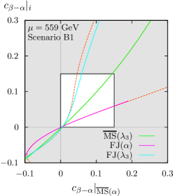
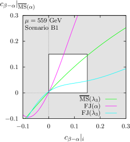
Figure 21: Panel (a): Conversion of the value of $c_{\beta-\alpha}$ from $\overline{\mathrm{MS}}$$(\alpha)$ to the other schemes for scenario B1 with the colour coding of Fig. 8. Panel (b) shows the conversion to the $\overline{\mathrm{MS}}$$(\alpha)$ scheme. The solid lines are obtained by solving the implicit equations numerically, the dashed orange lines in (a) correspond to the solution of (b) mirrored at the diagonal. The highlighted region shows the phenomenologically most relevant $c_{\beta-\alpha}$ region.

4.2.2 The running of $c_{\beta-\alpha}$

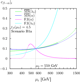
Figure 22: The running of $c_{\beta-\alpha}$ for benchmark scenario B1a in the $\overline{\mathrm{MS}}$($\alpha$) (blue), $\overline{\mathrm{MS}}$$(\lambda_{3})$ (green), FJ($\alpha$) (pink), and FJ($\lambda_{3}$) (turquoise) schemes. The breakdown of perturbativity ($\lambda_{k}^{\text{max}}/(4\pi)>1$) is indicated by changing the NLO curve to dotted lines.

The running of $c_{\beta-\alpha}$ in scenario  B1a is investigated in Fig. 22 analogously to the low-mass scenario for each renormalization scheme independently, without any conversion. The scale dependence of $c_{\beta-\alpha}(\mu_{\mathrm{r}})$ with $c_{\beta-\alpha}(\mu_{0})=0.1$ is computed from $\mu_{\mathrm{r}}=300\,\mathrm{GeV}$ to $1500\,\mathrm{GeV}$ using a Runge–Kutta method. We indicated regions where perturbativity is not valid with dotted lines using a slightly different perturbativity measure than in Figs. 6 and 7. Perturbativity is considered to be intact unless the largest of the quartic coupling parameters $\lambda_{k}$ of the Higgs potential with $k=1,\dots,5$ becomes too large, $\lambda_{k}^{\text{max}}/(4\pi)>1$. Compared to the previously used perturbativity measure, we found that with this measure a slightly larger part of the parameter space fulfills the perturbativity criterion.

In comparison to the low-mass scenario scenario (Fig. 9) the scale dependence in the FJ($\lambda_{3}$) scheme increases. For scales above the central scale we obtain large values of $c_{\beta-\alpha}$ for which predictions become unreliable. But also the FJ($\alpha$) scheme shows a remarkable behaviour as the alignment limit is approached for low as well as for high scales.

4.2.3 Scale variation of the width

We now turn to the calculation of the ${\mathrm{h}}{\to}4f$ width where we perform a scale variation similarly to the previous section in order to investigate the perturbative stability of the results and the validity of the central scale choice for scenario B1a. The scale is varied from $\mu_{\mathrm{r}}=300\,\mathrm{GeV}$ to $1000\,\mathrm{GeV}$, and the results are shown in Fig. 23 with one plot for each input prescription. First, the input values are converted to the target scheme, and afterwards the scale is varied. In regions where perturbativity is not valid ($\lambda_{k}^{\text{max}}/(4\pi)>1$) the NLO result is plotted with dotted lines. The results do not show such a clear and well behaved picture as for the low-mass scenario:

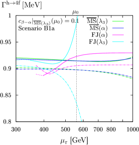
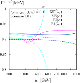
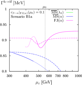
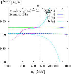
Figure 23: The ${\mathrm{h}}{\to}4f$ width at LO (dashed) and NLO EW (solid) for scenario B1a in dependence of the renormalization scale. The panels (a), (b), (c), and (d) correspond to input values defined in the $\overline{\mathrm{MS}}$$(\lambda_{3})$, $\overline{\mathrm{MS}}$$(\alpha)$, FJ($\alpha$), and FJ($\lambda_{3}$) schemes, respectively. The result is computed in all four different renormalization schemes after converting the input at NLO (also for the LO curves) and displayed using the colour code of Fig. 9. The breakdown of perturbativity ($\lambda_{k}^{\text{max}}/(4\pi)>1$) is indicated by changing the NLO curve to dotted lines.

• The $\overline{\mathrm{MS}}$$(\lambda_{3})$, Fig. 23, and the $\overline{\mathrm{MS}}$$(\alpha)$ input prescriptions, Fig. 23, yield similar results. In both cases, these schemes as target schemes show very good agreement, an extremum and a distinct plateau region in which the central scale fits perfectly. They only begin to deviate when perturbativity breaks down. The other renormalization schemes do not behave as nicely: The results of the FJ($\alpha$) scheme has a significant offset and drops dramatically for lower scales, until perturbativity breaks down at about $400\,\mathrm{GeV}$. The FJ($\lambda_{3}$) scheme suffers from the strong running and diverges at high scales as expected, while it shows relatively good (but not stable) agreement with the other schemes for lower scales.

• For input values defined in the FJ($\alpha$) scheme (Fig. 23), the conversion transports the large NLO corrections to all other schemes, so that perturbativity is not given at all, and all curves disagree. Together with the behaviour of the FJ($\alpha$) scheme in the other plots, we conclude that the perturbative predictions using the FJ($\alpha$) scheme are not trustworthy for this benchmark scenario.

• The FJ($\lambda_{3}$) input prescription (Fig. 23) seems to yield the best agreement between the schemes, however, the conversion to other renormalization schemes results in particularly small values for $c_{\beta-\alpha}$ and therefore corresponds in the other renormalization schemes to a scenario closer to the alignment limit. Such scenarios have smaller couplings and are perturbatively more stable, so that a better agreement is not surprising. For the ${\mathrm{h}}{\to}4f$ width in a high-mass scenario B1 with $c_{\beta-\alpha}=0.05$ shown in App. A.1 we observe a reduction of the scale dependence, the development of plateau regions for all schemes, and an overlap of the results from the different schemes.

In the computation of the relative renormalization scheme dependence at the central scale $\Delta_{\mathrm{RS}}$ only reliable renormalization schemes should be used. Therefore only the widths computed in the $\overline{\mathrm{MS}}$($\alpha$) and $\overline{\mathrm{MS}}$($\lambda_{3}$) schemes enter this calculation for which the result is shown in Tab. 6.

		$\overline{\mathrm{MS}}$$(\lambda_{3})$	$\overline{\mathrm{MS}}$$(\alpha)$	FJ($\alpha$)	FJ($\lambda_{3}$)
Scenario B1a	$\Delta^{\mathrm{LO}}_{\mathrm{RS}}$[%]	0.03(0)	0.04(0)	–	–
	$\Delta^{\mathrm{NLO}}_{\mathrm{RS}}$ [%]	0.02(0)	0.02(0)	–	–

Table 6: The variation $\Delta_{\mathrm{RS}}$ of the $\mathrm{h}{\to}4f$ width in scenario B1a at the central scale $\mu_{0}$ using the reliable renormalization schemes $\overline{\mathrm{MS}}$($\lambda_{3}$) and $\overline{\mathrm{MS}}$($\alpha$) (with NLO parameter conversions). The columns correspond to the schemes in which the input parameters are defined. Using parameters defined in the FJ($\alpha$) and FJ($\lambda_{3}$) schemes, the results are unreliable and a computation of $\Delta_{\mathrm{RS}}$ is not meaningful. The zeroes in brackets show that the integration errors are negligible.

Omitting the FJ schemes, our estimate of the scheme dependence is, thus, just the difference of the two $\overline{\mathrm{MS}}$ schemes, which is very small both at LO and NLO. Nevertheless a tendency towards a reduction of the scheme dependence is seen in the transition from LO to NLO. For the input values defined in one of the FJ schemes, this analysis cannot be performed as the results are unreliable.

4.2.4 $c_{\beta-\alpha}$ dependence

The ${\mathrm{h}}{\to}4f$ width of the Higgs decay as a function of positive $c_{\beta-\alpha}$ is shown for all combinations of input prescriptions and renormalization schemes in Fig. 24 at the scale $\mu_{0}$. The results from all schemes agree very well in the alignment limits, where $c_{\beta-\alpha}\to 0$. For $|c_{\beta-\alpha}|>0.05$, differences in the results obtained with different schemes after conversion from a common parameter input scheme start to become significant. The patterns observed in the investigation of the scale dependence recur. The dashed lines represent the LO result with an NLO input conversion, while at pure LO, i.e. without conversion, all renormalization schemes deliver identical results. The respective curve is the one where no conversion is necessary. The well-known $s_{\beta-\alpha}^{2}$ pattern can be observed at LO while the conversion into the FJ($\lambda_{3}$) scheme introduces large corrections leading to a breakdown (see Fig. 21), so that this scheme is only applicable for very low values of $c_{\beta-\alpha}$. The NLO results away from the alignment limit are more complicated:

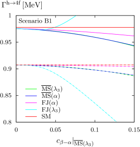
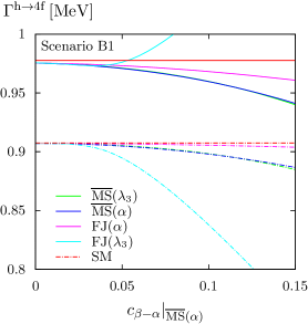
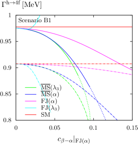
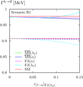
Figure 24: The ${\mathrm{h}}{\to}4f$ width at LO (dashed) and NLO EW+QCD (solid) for scenario B1 in dependence of $c_{\beta-\alpha}$. The panels (a), (b), (c), and (d) correspond to input values defined in the $\overline{\mathrm{MS}}$$(\lambda_{3})$, $\overline{\mathrm{MS}}$$(\alpha)$, FJ($\alpha$), and FJ($\lambda_{3}$) schemes, and they are converted to the other schemes at NLO (also for the LO curves). The result is displayed in all four schemes and for the SM using the colour code of Fig. 12. The breakdown of perturbativity ($\lambda_{k}^{\text{max}}/(4\pi)>1$) is visualized by using dotted lines for the NLO curve.

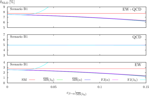
Figure 25: The relative NLO corrections of the full EW+QCD, the QCD, and the EW calculation in scenario B1. The input is defined in the $\overline{\mathrm{MS}}$$(\lambda_{3})$ scheme, and the corrections are computed in all four schemes which are displayed using the colour code of Fig. 12. For comparison the SM corrections with a SM Higgs-boson mass of $M_{\mathrm{h}}$ are shown as well.

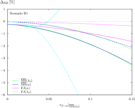
Figure 26: The $h{\to}4f$ width at LO with NLO conversion (dashed) and NLO EW+QCD (solid) in scenario B1, normalized to the respective SM values where the SM Higgs-boson mass is $M_{\mathrm{h}}$. The input is defined in the $\overline{\mathrm{MS}}$$(\lambda_{3})$ scheme, and the results in the four schemes are displayed using the colour code of Fig. 12.

• The $\overline{\mathrm{MS}}$$(\alpha)$ and the $\overline{\mathrm{MS}}$$(\lambda_{3})$ input prescriptions (Figs. 24,(b)) have similar characteristics which is due to the small shifts of the parameters in the conversion. The width in the $\overline{\mathrm{MS}}$$(\alpha)$ and the $\overline{\mathrm{MS}}$$(\lambda_{3})$ renormalization schemes agree very well, and the agreement improves from LO to NLO, as desired. The FJ($\alpha$) scheme (as target scheme) shows differences which can be explained by large higher-order terms shifting the input values towards the alignment limit (see Fig. 21). Owing to the large corrections at NLO, sizeable corrections beyond NLO are expected in the FJ schemes as well, i.e. for reliable predictions for the B1 scenario in the FJ schemes the inclusion of leading corrections beyond NLO should be calculated and taken into account.

• Using input values defined in the FJ($\alpha$) scheme, Fig. 24, expresses this problem more clearly. The large corrections spread to the other renormalization schemes and affect perturbativity in a negative way. But also within the FJ($\alpha$) scheme the corrections are large and differ from the $s_{\beta-\alpha}^{2}$ shape seen for other input variants. This confirms the conclusion of the previous section that predictions obtained using the FJ($\alpha$) are not reliable for this scenario.

• The good agreement of the renormalization schemes in the FJ($\lambda_{3}$) input prescription (Fig. 24) is based on the shift of the input values towards the alignment limit in the conversion. This shrinks the range effectively to $0<c_{\beta-\alpha}\;\raisebox{-3.00003pt}{$\stackrel{{\scriptstyle\displaystyle<}}{{\sim}}$}\;0.05$ for the other target schemes after the conversion and pushes the results together.

For the input defined in the $\overline{\mathrm{MS}}$$(\lambda_{3})$ scheme, the relative corrections separated in EW, QCD, and EW+QCD are shown in Fig. 25. Taking the input in the $\overline{\mathrm{MS}}$$(\alpha)$ scheme instead, the results look similar (not shown). The QCD corrections are similar for all schemes, because only the closed quark-loop diagrams in the ${\mathrm{h}}VV$ vertex corrections do not factorize from the SM LO amplitude with the coupling factor $\sin(\beta-\alpha)$, but the impact of those diagrams is small. In contrast to the low-mass scenario, the EW corrections decrease with increasing $c_{\beta-\alpha}$, so that the deviations from the SM shown in Fig. 26 are larger than in the low-mass case, although they remain below 2% for $c_{\beta-\alpha}<0.1$. The relative renormalization scheme dependence can only be applied using the $\overline{\mathrm{MS}}$($\alpha$) and $\overline{\mathrm{MS}}(\lambda_{3})$ schemes, as the results obtained using the two schemes involving FJ prescriptions are only reliable for very small $c_{\beta-\alpha}$. From Figs. 23,(b), one can see that the differences between the $\overline{\mathrm{MS}}$($\alpha$) and $\overline{\mathrm{MS}}(\lambda_{3})$ schemes decrease from LO to NLO, and the scheme dependence is reduced.

4.2.5 Partial widths for individual four-fermion states

The partial NLO widths, the relative corrections $\delta_{\mathrm{EW/QCD}}$, and the deviations from the SM, $\Delta_{\mathrm{SM}}^{\mathrm{LO/NLO}}$, are shown in Tab. 7 for benchmark scenario B1a using the $\overline{\mathrm{MS}}$$(\lambda_{3})$ renormalization scheme.

$\Big{|}$ Final state	$\Gamma^{{\mathrm{h}}{\to}4f}_{\mathrm{NLO}}$ [MeV]	$\delta_{\mathrm{EW}}$ [%]	$\delta_{\mathrm{QCD}}$ [%]	$\Delta_{\mathrm{SM}}^{\mathrm{NLO}}$ [%]	$\Delta_{\mathrm{SM}}^{\mathrm{LO}}$ [%]
inclusive ${\mathrm{h}}{\to}4f$	$0.95976(9)$	$1.88(0)$	$4.96(1)$	$-1.82(1)$	$-1.00(1)$
ZZ	$0.105308(7)$	$-0.48(0)$	$4.88(1)$	$-1.89(1)$	$-1.00(1)$
WW	$0.8596(1)$	$2.16(0)$	$5.02(1)$	$-1.81(2)$	$-1.00(1)$
WW/ZZ int.	$-0.00514(7)$	$0.3(2)$	$13(1)$	$-1(2)$	$-1(1)$
$\nu_{\mathrm{e}}{\mathrm{e}}^{+}\mu^{-}\bar{\nu}_{\mu}$	$0.010118(1)$	$2.19(0)$	$0.00$	$-1.85(2)$	$-1.00(2)$
$\nu_{\mathrm{e}}{\mathrm{e}}^{+}{\mathrm{u}}\bar{{\mathrm{d}}}$	$0.031471(5)$	$2.18(0)$	$3.77(1)$	$-1.82(2)$	$-1.00(2)$
${\mathrm{u}}\bar{{\mathrm{d}}}{\mathrm{s}}\bar{{\mathrm{c}}}$	$0.09772(2)$	$2.14(0)$	$7.52(2)$	$-1.79(3)$	$-1.00(2)$
$\nu_{\mathrm{e}}{\mathrm{e}}^{+}{\mathrm{e}}^{-}\bar{\nu}_{\mathrm{e}}$	$0.010113(1)$	$2.29(0)$	$0.00$	$-1.85(2)$	$-1.00(2)$
${\mathrm{u}}\bar{{\mathrm{d}}}{\mathrm{d}}\bar{{\mathrm{u}}}$	$0.09969(2)$	$2.02(0)$	$7.34(2)$	$-1.81(4)$	$-1.00(2)$
$\nu_{\mathrm{e}}\bar{\nu}_{\mathrm{e}}\nu_{\mu}\bar{\nu}_{\mu}$	$0.000941(0)$	$2.19(0)$	$0.00$	$-1.92(2)$	$-1.00(2)$
${\mathrm{e}}^{-}{\mathrm{e}}^{+}\mu^{-}\mu^{+}$	$0.000237(0)$	$0.49(1)$	$0.00$	$-1.94(2)$	$-1.00(1)$
$\nu_{\mathrm{e}}\bar{\nu}_{\mathrm{e}}\mu^{-}\mu^{+}$	$0.000474(0)$	$1.63(1)$	$0.00$	$-1.91(2)$	$-1.00(1)$
$\nu_{\mathrm{e}}\bar{\nu}_{\mathrm{e}}\nu_{\mathrm{e}}\bar{\nu}_{\mathrm{e}}$	$0.000564(0)$	$2.09(0)$	$0.00$	$-1.93(3)$	$-1.00(2)$
${\mathrm{e}}^{-}{\mathrm{e}}^{+}{\mathrm{e}}^{-}{\mathrm{e}}^{+}$	$0.000131(0)$	$0.31(1)$	$0.00$	$-1.92(2)$	$-1.00(1)$
$\nu_{\mathrm{e}}\bar{\nu}_{\mathrm{e}}{\mathrm{u}}\bar{{\mathrm{u}}}$	$0.001666(0)$	$-0.22(1)$	$3.75(1)$	$-1.89(2)$	$-1.00(1)$
$\nu_{\mathrm{e}}\bar{\nu}_{\mathrm{e}}{\mathrm{d}}\bar{{\mathrm{d}}}$	$0.002160(0)$	$0.88(1)$	$3.75(1)$	$-1.89(2)$	$-1.00(2)$
${\mathrm{e}}^{-}{\mathrm{e}}^{+}{\mathrm{u}}\bar{{\mathrm{u}}}$	$0.000839(0)$	$-0.70(1)$	$3.76(1)$	$-1.89(2)$	$-1.00(1)$
${\mathrm{e}}^{-}{\mathrm{e}}^{+}{\mathrm{d}}\bar{{\mathrm{d}}}$	$0.001080(0)$	$-0.35(1)$	$3.76(1)$	$-1.89(2)$	$-1.00(1)$
${\mathrm{u}}\bar{{\mathrm{u}}}{\mathrm{c}}\bar{{\mathrm{c}}}$	$0.002948(1)$	$-2.61(1)$	$7.51(2)$	$-1.86(3)$	$-1.00(1)$
${\mathrm{d}}\bar{{\mathrm{d}}}{\mathrm{d}}\bar{{\mathrm{d}}}$	$0.002537(1)$	$-1.20(0)$	$4.42(3)$	$-1.93(4)$	$-1.00(2)$
${\mathrm{d}}\bar{{\mathrm{d}}}{\mathrm{s}}\bar{{\mathrm{s}}}$	$0.004918(1)$	$-1.17(1)$	$7.50(2)$	$-1.86(3)$	$-1.00(2)$
${\mathrm{u}}\bar{{\mathrm{u}}}{\mathrm{s}}\bar{{\mathrm{s}}}$	$0.003823(1)$	$-1.48(1)$	$7.51(2)$	$-1.86(3)$	$-1.00(1)$
${\mathrm{u}}\bar{{\mathrm{u}}}{\mathrm{u}}\bar{{\mathrm{u}}}$	$0.001495(1)$	$-2.73(1)$	$4.12(3)$	$-1.95(5)$	$-1.00(1)$

Table 7: Partial widths for benchmark scenario B1a within the $\overline{\mathrm{MS}}$$(\lambda_{3})$ scheme.

The $\overline{\mathrm{MS}}$$(\alpha)$ scheme yields similar results which differ only at the permille level, whereas the other schemes are not reliable at this benchmark scenario. The widths are slightly smaller than in the low-mass scenario (see Sec. 4.1.5) in spite of the identical values of $c_{\beta-\alpha}$. The negative deviation from the SM rises to almost 2%, however, no final state accounts for distinctively large THDM effects that could be exploited in experiments.

In addition, the differential distributions of scenario B1a, as defined in Sec. 2, do not change the shape w.r.t. to the SM significantly. They are shown in App. A.2, together with the SM ones and the ones from scenario B2b. As observed in the low-mass scenario, for each four-fermion final state the difference between the ${\mathrm{h}}{\to}4f$ widths in the THDM and the SM resembles a constant shift in all distributions as well.

4.3 High-mass scenario B2

To complete the discussion of the high-mass scenario, we turn to negative values of $c_{\beta-\alpha}$ for which the parameter space is strongly reduced by perturbativity, stability, and unitarity constraints, leaving only a small branch around $\tan\beta=1.5$ and leading to scenario B2. Being in the vicinity of excluded parameter sets potentially affects the conversion, the scale dependence, and the reliability of the full results. Hence, similar to scenario B1, scenario B2 is well suited to actually address possible problems in that respect. We discuss the results in the same manner as scenario B1 for positive $c_{\beta-\alpha}$ above and present results for the less delicate case with $c_{\beta-\alpha}=-0.05$ in App. A.1.

4.3.1 Conversion of the input parameters

The conversion of the input parameter $c_{\beta-\alpha}$ between different renormalization schemes is shown in Fig. 27 for an enlarged range with $\overline{\mathrm{MS}}$($\alpha$) either as input or target scheme.

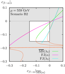
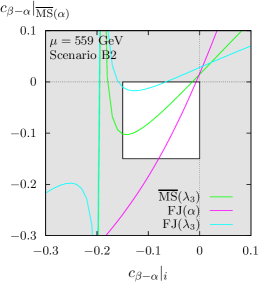
Figure 27: Panel (a): Conversion of the value of $c_{\beta-\alpha}$ from $\overline{\mathrm{MS}}$$(\alpha)$ to the other renormalization schemes for scenario B2 with the colour coding of Fig. 8. Panel (b) shows the conversion to the $\overline{\mathrm{MS}}$$(\alpha)$ scheme with the same colour coding. The solid lines are obtained by solving the implicit equations numerically, the dashed orange lines correspond to the solution of (b) mirrored at the diagonal. The linear approximation does not provide reasonable results. The highlighted region shows the phenomenologically most relevant $c_{\beta-\alpha}$ region.

The conversion into the $\overline{\mathrm{MS}}$($\alpha$) scheme shows several ominous features (Fig. 27(b)). First of all, divergences for the $\overline{\mathrm{MS}}(\lambda_{3})$ and FJ($\lambda_{3}$) schemes occur at $c_{\beta-\alpha}\approx-0.19$. We have seen such a divergence already in the low-mass scenario outside of the relevant region (c.f. Sec. 4.1.1), which is caused by the singularity at $c_{2\alpha}=0$. Since the ratio of the vacuum expectation values is lower in this scenario, the divergence moves towards the alignment limit and closer to the relevant region. It affects the conversion for $c_{\beta-\alpha}<-0.15$ in the $\overline{\mathrm{MS}}(\lambda_{3})$ and FJ($\lambda_{3}$) schemes, so that such values should be taken with care. If experimental observations favour this region of parameter space, it becomes necessary to redefine the renormalization scheme and choose a different Higgs self-coupling parameter (e.g. $\lambda_{1}$) or a combination (e.g. $\lambda_{1}+\lambda_{2}$) as independent parameter renormalized in $\overline{\mathrm{MS}}$. The singularity then appears in other parameter regions and allows for predictions with $c_{\beta-\alpha}\;\raisebox{-3.00003pt}{$\stackrel{{\scriptstyle\displaystyle<}}{{\sim}}$}\;-0.15$. Not only the schemes involving $\lambda_{3}$ are problematic, but also the conversion from the FJ($\alpha$) scheme, as large shifts indicate problems with the perturbative expansion, analogous to scenario B1.

Figure 27 shows the results for the “inverse” conversion from the $\overline{\mathrm{MS}}$($\alpha$) scheme, together with the inverse of (b) obtained graphically by mirroring the curves at the diagonal (dashed orange). Note that the linearized approximation for the conversion would involve large uncertainties here. Although the comparison of these curves projects the reduction of the conversion to one dimension (spanned by $c_{\beta-\alpha}$), which is thus not exact, it gives a quick overview over the convergence of the numerical solution. As expected, the singularity in the relation between $\lambda_{3}$ and $\alpha$ reduces the domain of definition for the conversion in Fig. 27 to $c_{\beta-\alpha}|_{\overline{\mathrm{MS}}(\alpha)}>-0.1$ for the $\overline{\mathrm{MS}}(\lambda_{3})$ scheme and $c_{\beta-\alpha}|_{\overline{\mathrm{MS}}(\alpha)}>-0.05$ for the FJ($\lambda_{3}$) scheme. Values outside this domain cannot be converted into these schemes, and solid predictions cannot be made there.

4.3.2 The running of $c_{\beta-\alpha}$

The running of $c_{\beta-\alpha}(\mu_{\mathrm{r}})$ with $c_{\beta-\alpha}(\mu_{0})=-0.1$ is computed from $\mu_{\mathrm{r}}=300\,\mathrm{GeV}$ to $1500\,\mathrm{GeV}$ with a Runge–Kutta method for scenario B2b. The result is shown in Fig. 28 for each renormalization scheme without any conversion.

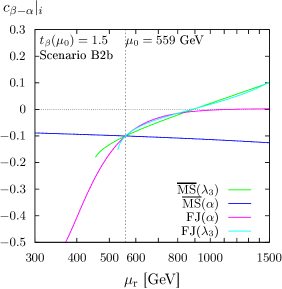
Figure 28: The running of $c_{\beta-\alpha}$ for scenario B2b for the different schemes in the colour code of Fig. 9.

The curves look similar to the ones of the low-mass scenario pictured in Fig. 9 (although the range of $\mu_{\mathrm{r}}$ is different) and we observe the same effects: the truncation of the $\overline{\mathrm{MS}}(\lambda_{3})$ and FJ($\lambda_{3}$) schemes, but also the strong scale dependence of the FJ($\alpha$) scheme and the good stability of the $\overline{\mathrm{MS}}$($\alpha$) scheme.

4.3.3 Scale variation of the width

For the ${\mathrm{h}}{\to}4f$ width we again perform a scale variation in order to estimate theoretical uncertainties and to motivate the central scale choice. The method is as described in Sec. 4.1.3, and the results are shown in Fig. 29.

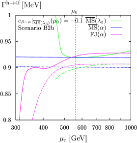
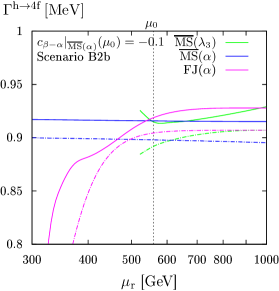
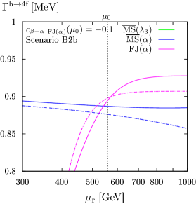
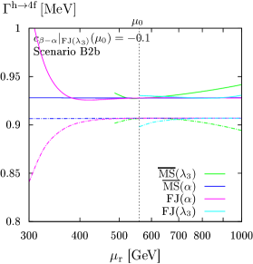
Figure 29: The ${\mathrm{h}}{\to}4f$ width at LO (dashed) and NLO EW (solid) for scenario B2b in dependence of the renormalization scale. The panels (a), (b), (c), and (d) correspond to input values defined in the $\overline{\mathrm{MS}}$$(\lambda_{3})$, $\overline{\mathrm{MS}}$$(\alpha)$, FJ($\alpha$), and FJ($\lambda_{3}$) schemes, respectively. For each of them, the result is computed in all four different renormalization schemes after converting the input at NLO (also for the LO curves) and displayed using the colour code of Fig. 9. The FJ($\lambda_{3}$) scheme is not defined as target schemes due to the singular relation between $\alpha$ and $\lambda_{3}$.

The FJ($\lambda_{3}$) renormalization scheme is not included as target scheme here, since it is not possible to convert input values to it for $c_{\beta-\alpha}=-0.1$ (see Fig. 27), however, it can be used when the input values are defined in it. The observations correspond in the most cases to the ones of scenario B1:

• The first two plots using parameters defined in the $\overline{\mathrm{MS}}(\lambda_{3})$ (Fig. 29) and $\overline{\mathrm{MS}}$($\alpha$) (Fig. 29) schemes show, as in the previous scenarios, similar characteristics. The result obtained with the $\overline{\mathrm{MS}}$($\alpha$) renormalization scheme shows almost no scale dependence, and its value agrees with the extremum of the the $\overline{\mathrm{MS}}(\lambda_{3})$ renormalization scheme which lies at the central scale. However, through the truncation of the running a broad plateau region cannot be observed for the latter scheme with input in $\overline{\mathrm{MS}}$$(\alpha)$. The width in the FJ($\alpha$) scheme is consistent with the results of the $\overline{\mathrm{MS}}(\lambda_{3})$ and $\overline{\mathrm{MS}}$($\alpha$) schemes at the central scale, but shows an offset at the plateau and decreases for scales below $\mu_{0}$, as expected from the running of $c_{\beta-\alpha}$.

• The results using the FJ($\alpha$) input prescription (Fig. 29) are not conclusive, since large corrections from the conversion spread to all other schemes.

• The scale variation of the FJ($\lambda_{3}$) input prescription (Fig. 29) corresponds again to an aligned scenario in the other renormalization schemes. Closer to the alignment, the renormalization scheme dependence decreases, which can also be seen from the separate scale variation of a more aligned scenario with $c_{\beta-\alpha}=-0.05$ given in App. A.1.

Generically, we obtain a somewhat better improvement compared to benchmark scenario B1a, which probably originates from smaller perturbativity measures (see Fig. 6). The central scale of Eq. (3.4) is a justifiable choice and suggests that this scale is a good candidate for the THDM Higgs decay into four fermions in general, although the scale choice should be better checked for consistency in any new scenario. The renormalization schemes $\overline{\mathrm{MS}}$($\alpha$) and $\overline{\mathrm{MS}}{}(\lambda_{3})$ yield trustworthy and comparable results, even though one should respect the domain of definition of the latter. Results based on an input in the FJ($\alpha$) scheme do not seem reliable; the FJ($\lambda_{3}$) scheme cannot even be applied for this input procedure. The renormalization scheme dependence at the central scale reduces from LO to NLO as shown in Tab. 8. For the input renormalization schemes $\overline{\mathrm{MS}}$$(\lambda_{3})$ and $\overline{\mathrm{MS}}$$(\alpha)$, we did not take the FJ($\lambda_{3}$) scheme into account when evaluating the renormalization scheme dependence while for the input scheme FJ($\lambda_{3}$), all four renormalization schemes have been considered. This corresponds to the results shown in Fig. 29.

		$\overline{\mathrm{MS}}$$(\lambda_{3})$	$\overline{\mathrm{MS}}$$(\alpha)$	FJ($\alpha$)	FJ($\lambda_{3}$)
Scenario B2b	$\Delta^{\mathrm{LO}}_{\mathrm{RS}}$[%]	0.81(0)	1.40(0)	–	0.99(0)
	$\Delta^{\mathrm{NLO}}_{\mathrm{RS}}$ [%]	0.31(0)	0.46(0)	–	0.25(0)

Table 8: The variation $\Delta_{\mathrm{RS}}$ of the $\mathrm{h}{\to}4f$ width in scenario B2b at the central scale $\mu_{0}$ using the renormalization schemes $\overline{\mathrm{MS}}$($\alpha$), $\overline{\mathrm{MS}}$($\lambda_{3}$), and FJ($\alpha$) (with NLO parameter conversions). The columns correspond to the schemes in which the input parameters are defined. Using parameters defined in the FJ($\alpha$) scheme, the results are unreliable, and a computation of $\Delta_{\mathrm{RS}}$ is not meaningful. The zeroes in brackets show that the integration errors are negligible.

4.3.4 $c_{\beta-\alpha}$ dependence

The dependence of the ${\mathrm{h}}{\to}4f$ width on $c_{\beta-\alpha}$ is shown for the different input prescriptions in the four panels of Fig. 30, for all renormalization schemes.

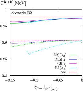
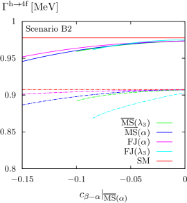
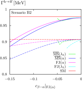
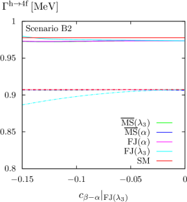
Figure 30: The ${\mathrm{h}}{\to}4f$ width at LO (dashed) and NLO EW+QCD (solid) for scenario B2 in dependence of $c_{\beta-\alpha}$. The panels (a), (b), (c), and (d) correspond to input values defined in the $\overline{\mathrm{MS}}$$(\lambda_{3})$, $\overline{\mathrm{MS}}$$(\alpha)$, FJ($\alpha$), and FJ($\lambda_{3}$) schemes, respectively. The input values are converted to the desired target scheme (colour code of Fig. 9) in which the calculation is performed. The SM prediction is shown for comparison in red.

Close to the alignment limit, $-0.05\;\raisebox{-3.00003pt}{$\stackrel{{\scriptstyle\displaystyle<}}{{\sim}}$}\;c_{\beta-\alpha}<0$, the results from different renormalization schemes agree nicely. Away from this limit, however, the results deviate significantly, demanding some discussion:

• The curves obtained using the $\overline{\mathrm{MS}}(\lambda_{3})$ and the FJ($\lambda_{3}$) input prescriptions, Fig. 30 and Fig. 30, show the largest deviation from the $s_{\beta-\alpha}^{2}$ dependence of the LO width because of the large corrections inherited from the parameter conversions to the other schemes, which were observed in Fig. 27. Defining the input in the FJ($\lambda_{3}$) scheme, the NLO width even slightly increases with smaller $c_{\beta-\alpha}$ values, since the corresponding $c_{\beta-\alpha}$ value in the $\overline{\mathrm{MS}}(\alpha)$ scheme stays close to the alignment limit. Owing to the large conversion effects, especially the predictions in the FJ($\lambda_{3}$) scheme involve large uncertainties, which could only be reduced by systematically including the leading effects beyond NLO.

• Using input values defined in the $\overline{\mathrm{MS}}$($\alpha$) scheme yields the smooth curves of Fig. 30 which have the expected $s_{\beta-\alpha}^{2}$ shape. The relative renormalization scheme dependence reduces from LO to NLO, while the breakdown of the $\overline{\mathrm{MS}}(\lambda_{3})$ and FJ($\lambda_{3}$) schemes is manifest, since values of $c_{\beta-\alpha}$ smaller than $\sim-0.1$ or $\sim-0.05$ in the $\overline{\mathrm{MS}}(\alpha)$ scheme cannot be converted into the $\overline{\mathrm{MS}}(\lambda_{3})$ or FJ($\lambda_{3}$) schemes, respectively (cf. Fig. 27).

• The FJ$(\alpha)$ input prescription shows largest deviations from the SM as large NLO contributions spread to the other schemes through the conversion, shifting the values away from the alignment limit and increasing the deviations from the SM prediction.

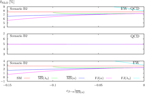
Figure 31: The relative NLO EW+QCD, QCD, and EW corrections to the ${\mathrm{h}}{\to}4f$ width in scenario B2. The input is defined in the $\overline{\mathrm{MS}}$$(\alpha)$ scheme and the corrections are computed in all four schemes which are displayed together with the SM corrections using the colour code of Fig. 12.

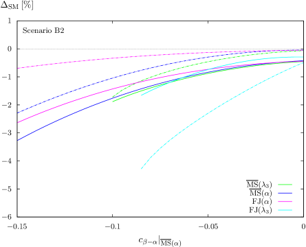
Figure 32: The ${\mathrm{h}}{\to}4f$ width at LO (dashed) and NLO EW+QCD (solid) in the THDM scenario B2, normalized to the respective SM values. The input is defined in the $\overline{\mathrm{MS}}$$(\alpha)$ scheme, and the corrections are computed in all four schemes which are displayed using the colour code of Fig. 12.

However, all results show a significantly better agreement between the renormalization schemes at NLO than for LO for all regions including the problematic ones, suggesting that the perturbative expansion works for this scenario in the vicinity of our central scale $\mu_{0}$ in spite of partially large NLO terms. As the $\overline{\mathrm{MS}}(\lambda_{3})$ scheme has a limited region of applicability, we show in Fig. 31 the relative corrections using the $\overline{\mathrm{MS}}$($\alpha$) scheme, which is reliable over the whole scan range. The QCD corrections are similar to the SM and renormalization scheme independent, while the EW corrections show the breakdown of the $\overline{\mathrm{MS}}(\lambda_{3})$ and FJ($\lambda_{3}$) schemes. The difference between the FJ($\alpha$) and the $\overline{\mathrm{MS}}$($\alpha$) schemes is slightly larger than in the low-mass case, however, the sizes of the corrections are almost equal. This results in similar deviations from the SM as can be seen by comparing Fig. 32 with Fig. 15 (it should, however, be noted that a different input scheme has been used), so that it is difficult to distinguish these scenarios using the Higgs decay into four fermions.

4.3.5 Partial widths for individual four-fermion states

We give the partial widths in Tab. 9 for scenario B2b in the $\overline{\mathrm{MS}}$($\alpha$) scheme, as this scheme provides reliable results for $c_{\beta-\alpha}=-0.1$.

$\Big{|}$ Final state	$\Gamma^{{\mathrm{h}}{\to}4f}_{\mathrm{NLO}}$ [MeV]	$\delta_{\mathrm{EW}}$ [%]	$\delta_{\mathrm{QCD}}$ [%]	$\Delta_{\mathrm{SM}}^{\mathrm{NLO}}$ [%]	$\Delta_{\mathrm{SM}}^{\mathrm{LO}}$ [%]
inclusive ${\mathrm{h}}{\to}4f$	$0.96086(9)$	$1.99(0)$	$4.97(1)$	$-1.71(1)$	$-1.00(1)$
ZZ	$0.105584(7)$	$-0.22(0)$	$4.90(1)$	$-1.63(1)$	$-1.00(1)$
WW	$0.8604(1)$	$2.26(0)$	$5.02(1)$	$-1.72(2)$	$-1.00(1)$
WW/ZZ int.	$-0.00509(7)$	$0.5(2)$	$11(1)$	$-2(2)$	$-1(1)$
$\nu_{\mathrm{e}}{\mathrm{e}}^{+}\mu^{-}\bar{\nu}_{\mu}$	$0.010128(1)$	$2.29(0)$	$0.00$	$-1.76(2)$	$-1.00(2)$
$\nu_{\mathrm{e}}{\mathrm{e}}^{+}{\mathrm{u}}\bar{{\mathrm{d}}}$	$0.031499(5)$	$2.28(0)$	$3.77(1)$	$-1.73(2)$	$-1.00(2)$
${\mathrm{u}}\bar{{\mathrm{d}}}{\mathrm{s}}\bar{{\mathrm{c}}}$	$0.09781(2)$	$2.23(0)$	$7.52(2)$	$-1.70(3)$	$-1.00(2)$
$\nu_{\mathrm{e}}{\mathrm{e}}^{+}{\mathrm{e}}^{-}\bar{\nu}_{\mathrm{e}}$	$0.010123(1)$	$2.39(0)$	$0.00$	$-1.75(2)$	$-1.00(2)$
${\mathrm{u}}\bar{{\mathrm{d}}}{\mathrm{d}}\bar{{\mathrm{u}}}$	$0.09981(2)$	$2.12(0)$	$7.37(2)$	$-1.69(4)$	$-1.00(2)$
$\nu_{\mathrm{e}}\bar{\nu}_{\mathrm{e}}\nu_{\mu}\bar{\nu}_{\mu}$	$0.000944(0)$	$2.46(0)$	$0.00$	$-1.67(2)$	$-1.00(2)$
${\mathrm{e}}^{-}{\mathrm{e}}^{+}\mu^{-}\mu^{+}$	$0.000237(0)$	$0.74(1)$	$0.00$	$-1.69(2)$	$-1.00(1)$
$\nu_{\mathrm{e}}\bar{\nu}_{\mathrm{e}}\mu^{-}\mu^{+}$	$0.000475(0)$	$1.89(1)$	$0.00$	$-1.66(2)$	$-1.00(1)$
$\nu_{\mathrm{e}}\bar{\nu}_{\mathrm{e}}\nu_{\mathrm{e}}\bar{\nu}_{\mathrm{e}}$	$0.000566(0)$	$2.35(0)$	$0.00$	$-1.68(3)$	$-1.00(2)$
${\mathrm{e}}^{-}{\mathrm{e}}^{+}{\mathrm{e}}^{-}{\mathrm{e}}^{+}$	$0.000131(0)$	$0.57(1)$	$0.00$	$-1.66(2)$	$-1.00(1)$
$\nu_{\mathrm{e}}\bar{\nu}_{\mathrm{e}}{\mathrm{u}}\bar{{\mathrm{u}}}$	$0.001670(0)$	$0.04(1)$	$3.75(1)$	$-1.65(2)$	$-1.00(1)$
$\nu_{\mathrm{e}}\bar{\nu}_{\mathrm{e}}{\mathrm{d}}\bar{{\mathrm{d}}}$	$0.002165(0)$	$1.13(0)$	$3.75(1)$	$-1.65(2)$	$-1.00(2)$
${\mathrm{e}}^{-}{\mathrm{e}}^{+}{\mathrm{u}}\bar{{\mathrm{u}}}$	$0.000841(0)$	$-0.45(1)$	$3.76(1)$	$-1.65(2)$	$-1.00(1)$
${\mathrm{e}}^{-}{\mathrm{e}}^{+}{\mathrm{d}}\bar{{\mathrm{d}}}$	$0.001082(0)$	$-0.09(1)$	$3.76(1)$	$-1.65(2)$	$-1.00(1)$
${\mathrm{u}}\bar{{\mathrm{u}}}{\mathrm{c}}\bar{{\mathrm{c}}}$	$0.002955(1)$	$-2.36(1)$	$7.51(2)$	$-1.63(3)$	$-1.00(1)$
${\mathrm{d}}\bar{{\mathrm{d}}}{\mathrm{d}}\bar{{\mathrm{d}}}$	$0.002548(1)$	$-0.94(0)$	$4.59(3)$	$-1.52(4)$	$-1.00(2)$
${\mathrm{d}}\bar{{\mathrm{d}}}{\mathrm{s}}\bar{{\mathrm{s}}}$	$0.004930(1)$	$-0.92(0)$	$7.50(2)$	$-1.63(3)$	$-1.00(2)$
${\mathrm{u}}\bar{{\mathrm{u}}}{\mathrm{s}}\bar{{\mathrm{s}}}$	$0.003832(1)$	$-1.23(1)$	$7.51(2)$	$-1.62(3)$	$-1.00(1)$
${\mathrm{u}}\bar{{\mathrm{u}}}{\mathrm{u}}\bar{{\mathrm{u}}}$	$0.001502(0)$	$-2.48(1)$	$4.35(3)$	$-1.49(5)$	$-1.00(1)$

Table 9: Partial widths for benchmark scenario B2b in the $\overline{\mathrm{MS}}$$(\alpha)$ renormalization scheme.

All the partial widths are similar to the ones of the low-mass scenario Ab (Tab. 5) in size (note, however, different input schemes have been used). This observation applies to the EW and QCD corrections and to the differences to the SM predictions as well. Again, there is no final state particularly sensitive to the THDM contributions. The differential distributions analogous to Sec. 4.1.6 are shown together with the distributions of the high-mass benchmark scenario B1 in App. A.2 and yield no significant shape distortion w.r.t. the SM, but only constant shifts that match the deviation of the respective partial widths.

4.4 Different THDM types

In this section, we compare the ${\mathrm{h}}{\to}4f$ decay widths of the Type I, Type II, lepton specific, and flipped THDMs for the two scenarios Aa and B1a using the $\overline{\mathrm{MS}}$$(\lambda_{3})$ renormalization scheme. We do not expect large differences in the results, because the considered THDM versions differ only in the Yukawa couplings of Higgs bosons to the leptons and to down-type quarks, which are not enhanced by large fermion masses. The by far largest contributions involving Yukawa couplings, however, result from diagrams with top-quark–Higgs couplings, which are identical in all four THDM versions for the ${\mathrm{h}}{\to}4f$ processes with massless external fermions. The results are shown in Tab. 10 with the numerical errors in parentheses, confirming our expectation:

Scenario Aa
Model	$\Gamma^{{\mathrm{h}}{\to}4f}_{\mathrm{NLO}}$ [MeV]	$\delta_{\mathrm{EW}}[\%]$	$\delta_{\mathrm{QCD}}[\%]$
Type I	$0.96730(7)$	$2.711(1)$	$4.962(5)$
Type II	$0.96729(7)$	$2.711(1)$	$4.962(5)$
Lepton-specific	$0.96730(7)$	$2.711(1)$	$4.962(5)$
Flipped	$0.96729(7)$	$2.711(1)$	$4.962(5)$
Scenario B1a
Model	$\Gamma^{{\mathrm{h}}{\to}4f}_{\mathrm{NLO}}$ [MeV]	$\delta_{\mathrm{EW}}[\%]$	$\delta_{\mathrm{QCD}}[\%]$
Type I	$0.95981(7)$	$1.878(3)$	$4.961(5)$
Type II	$0.95980(7)$	$1.879(3)$	$4.959(5)$
Lepton-specific	$0.95981(7)$	$1.878(3)$	$4.961(5)$
Flipped	$0.95980(7)$	$1.879(3)$	$4.959(5)$

Table 10: The ${\mathrm{h}}{\to}4f$ widths for the different types of THDM for scenarios Aa and B1a using the $\overline{\mathrm{MS}}$$(\lambda_{3})$ renormalization scheme. The numerical errors are given in parentheses.

The differences originating from the different THDM types in the NLO corrections are below a permille and not even significant over the integration error (although we employ large statistics with 190 million phase-space points). The ${\mathrm{h}}{\to}4f$ decay observables are, thus, rather insensitive to the different types of THDMs, so that our predictions are universally valid for all types.

4.5 Benchmark plane

For the benchmark plane scenario defined in Sec. 3 we analyze only the relative deviation $\Delta_{\mathrm{SM}}$ of the ${\mathrm{h}}{\to}4f$ width with respect to the SM in the $\overline{\mathrm{MS}}(\lambda_{3})$ scheme. At LO, this is $-0.01$ as $c_{\beta-\alpha}=0.1$ is kept constant. The NLO corrections differentiate this picture as they are dependent on both the heavy-Higgs-boson masses and $\tan{\beta}$. We show the result for a wide range in the $(M_{\mathrm{H}},\tan{\beta})$ plane in Fig. 33 where the colour of the parameter point indicates the deviation $\Delta_{\mathrm{SM}}^{\mathrm{NLO}}$ and gray areas are excluded by perturbativity constraints ($\lambda_{k}^{\text{max}}/(4\pi)>1$).

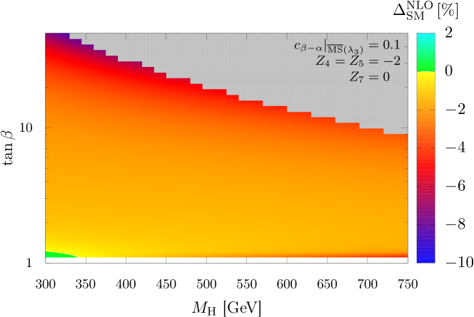
Figure 33: The relative deviation $\Delta_{\mathrm{SM}}$ of the ${\mathrm{h}}{\to}4f$ width w.r.t. the SM at NLO for the benchmark plane scenario in the $\overline{\mathrm{MS}}(\lambda_{3})$ scheme. Gray areas are excluded by non-perturbativity while the size of the deviations is indicated by the colour. We interpolate linearly between computed points to obtain a smooth picture.

We interpolate between the computed parameter points to obtain a smooth result, however, the original grid can be seen at the border between the computed area and the area excluded by non-perturbativity. The major deviation is between $0$ and $-5\%$ and grows in magnitude with increasing $\tan{\beta}$. For very large values of this parameter and close to the perturbative exclusion, values up to $-8\%$ occur. Very interesting is also the region with a small $\tan{\beta}$, as very small enhancements with respect to the SM can be found around $M_{\mathrm{H}}=300\,\mathrm{GeV}$ (displayed in green). However, this region has a strong mass dependence because for large masses the negative corrections become $-5$%. We note that this effect is also visible using the $\overline{\mathrm{MS}}$($\alpha$) scheme and therefore not an artifact of the singularity of the $\overline{\mathrm{MS}}(\lambda_{3})$ scheme.

4.6 Baryogenesis

In this section we discuss the results for the benchmark sets BP3 [64, 37], as defined in Sec. 3, which were proposed as a possible solution to the problem of baryogenesis. The results shown in Tab. 11 are computed in the $\overline{\mathrm{MS}}(\lambda_{3})$ scheme without considering the other schemes. In spite of the large distance to the alignment limit, the small heavy-Higgs-boson masses render both scenarios perturbatively stable with perturbativity measures of about $0.4$. Already at tree level we observe a large negative deviation from the SM caused by the large values for $c_{\beta-\alpha}$ suppressing the ${\mathrm{h}}VV$ coupling. These effects are enhanced at NLO for which we observe an increase of the negative deviation by 3 percentage points. This should be used in experiments measuring the Higgs decay into four fermions to put stronger bounds on these scenarios.

	$\Gamma^{{\mathrm{h}}{\to}4f}_{\mathrm{NLO}}$ [MeV]	$\delta_{\mathrm{EW}}[\%]$	$\delta_{\mathrm{QCD}}[\%]$	$\Delta_{\mathrm{SM}}^{\mathrm{LO}}[\%]$	$\Delta_{\mathrm{SM}}^{\mathrm{NLO}}[\%]$
$\mathrm{BP3}_{B1}$	$0.86042(8)$	$-0.76(0)$	$4.96(1)$	$-9.00(1)$	$-11.98(1)$
$\mathrm{BP3}_{B2}$	$0.70240(7)$	$-1.73(0)$	$4.94(1)$	$-25.00(1)$	$-28.15(1)$

Table 11: The ${\mathrm{h}}{\to}4f$ widths in the $\overline{\mathrm{MS}}(\lambda_{3})$ scheme, including the EW and QCD corrections in the benchmark scenarios $\mathrm{BP3}_{B1,B2}$ (with the numerical errors in parentheses). The last two columns show the deviation from the SM prediction at LO and NLO.

4.7 Fermiophobic heavy Higgs

The results for the fermiophobic heavy Higgs scenario [10, 37], as defined in Sec. 3, are shown in Tab. 12 for the $\overline{\mathrm{MS}}(\lambda_{3})$ scheme. The three scenarios have a perturbativity measure of $\lambda_{k}^{\text{max}}=0.6$ and differ by their value of $\tan{\beta}$. Note that all those scenarios are close to the alignment limit, so that the SM width is almost reached at LO. The NLO corrections increase the deviation from the SM by about $1\%$ for all scenarios.

	$\Gamma^{{\mathrm{h}}{\to}4f}_{\mathrm{NLO}}$ [MeV]	$\delta_{\mathrm{EW}}[\%]$	$\delta_{\mathrm{QCD}}[\%]$	$\Delta_{\mathrm{SM}}^{\mathrm{LO}}[\%]$	$\Delta_{\mathrm{SM}}^{\mathrm{NLO}}[\%]$
$\mathrm{BP6}_{a}$	$0.96456(9)$	$1.40(0)$	$4.97(1)$	$-0.06(1)$	$-1.33(1)$
$\mathrm{BP6}_{b}$	$0.96304(9)$	$1.43(0)$	$4.97(1)$	$-0.25(1)$	$-1.49(1)$
$\mathrm{BP6}_{c}$	$0.95701(9)$	$1.56(0)$	$4.97(1)$	$-0.99(1)$	$-2.10(1)$

Table 12: The ${\mathrm{h}}{\to}4f$ widths the $\overline{\mathrm{MS}}(\lambda_{3})$ scheme including the EW and QCD corrections of the benchmark scenarios $\mathrm{BP6}_{a{-}c}$ (with the numerical errors in parentheses). The last two columns show the deviation from the SM prediction at LO and NLO.

5 Conclusions

We have investigated the decay processes ${\mathrm{h}}\to{\mathrm{W}}{\mathrm{W}}/{\mathrm{Z}}{\mathrm{Z}}\to 4f$ in the THDM, where we identify the light neutral CP-even Higgs boson ${\mathrm{h}}$ with the discovered Higgs boson of mass $M_{\mathrm{h}}=125\,\mathrm{GeV}$. This signature contributed to the discovery of the Higgs boson and is important in the experimental investigation of the properties of the Higgs boson, such as the measurement of its couplings to other particles. The corresponding decay observables allow for precision tests of the SM and, thus, contribute to the search for any deviations from SM predictions. The calculation of strong and electroweak corrections in specific SM extensions, such as the one presented in this paper in the THDM, is an important theory input to successful data analyses.

In our phenomenological discussion of numerical results, we have considered several THDM benchmark scenarios proposed by the LHC Higgs Cross Section Working Group. For the investigated scenarios, we generally observe that the THDM predictions for the ${\mathrm{h}}{\to}4f$ width are bounded from above by the SM prediction and that the deviations from the SM typically increase at NLO, which might be used to improve exclusion limits in the THDM parameter space. The individual partial widths show similar deviations from the SM for all final states, but the shapes of differential distributions are not distorted by THDM contributions, so that the latter are not helpful to identify traces of the THDM. Moreover, we find that the ${\mathrm{h}}{\to}4f$ widths do not discriminate between different types of THDMs (Types I and II, lepton-specific and flipped).

We employ different renormalization schemes to define the THDM (i.e. the precise physical meaning of its input parameters) at NLO. Specifically, we apply four different schemes which have in common that we use as many as possible input quantities that are directly accessible by experiment, such as the (on-shell) masses of all five Higgs bosons of the THDM. For the remaining three free parameters, which are Higgs mixing angles and Higgs self-couplings, we adopt $\overline{\mathrm{MS}}$ prescriptions in four different variants. In detail, the $\overline{\mathrm{MS}}(\alpha)$ scheme defines the two mixing angles $\alpha$ and $\beta$ of the CP-even and CP-odd Higgs bosons, respectively, as well as the quartic Higgs self-coupling parameter $\lambda_{5}$ in the $\overline{\mathrm{MS}}$ scheme, and FJ$(\alpha)$ is a modified variant of this scheme with a different treatment of tadpole contributions in such a way that no gauge dependence between input parameters and predicted observables is introduced. Similarly, we define the two schemes $\overline{\mathrm{MS}}(\lambda_{3})$ and FJ$(\lambda_{3})$ in which we replace the angle $\alpha$ by another self-coupling parameter $\lambda_{3}$ as input. For a consistent comparison of results obtained in the different renormalization schemes, the $\overline{\mathrm{MS}}$-renormalized parameters have to be properly converted between the schemes. Depending on the scenario, we observe sizeable conversion effects on those parameters which can grow very large in scenarios close to the experimental exclusion limits or in parameter regions where perturbative stability deteriorates. These corrections, in particular, imply that the so-called alignment limit, in which one of the CP-even Higgs bosons of the THDM is SM-like, corresponds to different Higgs mixing angles in different renormalization schemes (even to different angles of a given renormalization scheme if the renormalization scale is changed). This shows that a proper definition of parameters at NLO is mandatory in future predictions and parameter fits in the THDM when precision is at stake.

While we observe a reduction of both the renormalization scheme and renormalization scale dependence of the ${\mathrm{h}}{\to}4f$ width in the transition from LO to NLO as long as all Higgs-boson masses are moderate and the distance to the alignment limit is not too large, some renormalization schemes prove unreliable, i.e. prone to large corrections beyond NLO, for scenarios with heavy Higgs bosons or away from the alignment limit. Generically, the comparison of the different schemes reveals that the gauge-dependent $\overline{\mathrm{MS}}$($\alpha$) scheme shows a minimal scale dependence which reflects good perturbative stability. The $\overline{\mathrm{MS}}(\lambda_{3})$ scheme deviates only slightly from the former, yields reliable results and in addition is gauge independent at one loop in $R_{\xi}$ gauges. However, a singular region in the THDM parameter space exists in which the scheme is not defined. If this region is experimentally favoured, it is necessary to redefine the scheme by replacing $\lambda_{3}$ by another scalar self-interaction $\lambda_{k\neq 3}$, so that the singularity is avoided. The gauge-independent FJ schemes partially suffer from large corrections and can only be applied for parameter points with sufficiently small coupling factors. Since the different schemes do not yield reliable results for all scenarios, self-consistency checks should be performed for every scenario when higher-order corrections are computed. In cases where NLO fails to be predictive, NLO calculations should be stabilized upon including the leading (renormalization-scheme-specific) corrections beyond NLO, a task that is, however, beyond the scope of this paper.

In more detail, in the low-mass scenario with a heavy CP-even Higgs boson of $300\,\mathrm{GeV}$ we obtain textbook-like results for the scale dependence, i.e. an improvement of the scale uncertainty and a reduction of differences between all four renormalization schemes at NLO, which indicates that perturbation theory works well. The deviation of the ${\mathrm{h}}{\to}4f$ width from the SM prediction are, depending on the parameter set, between 0% and $-6$%, to which the NLO corrections contribute about $1{-}2$%. In high-mass scenarios with heavy Higgs bosons with masses of about $600\,\mathrm{GeV}$, the coupling factors are larger, resulting in less predictive results and larger differences between the renormalization schemes. Close to the alignment limit, the results of all four schemes are self-consistent and nicely agree, but away from it differences occur. While the $\overline{\mathrm{MS}}$($\alpha$) and the $\overline{\mathrm{MS}}(\lambda_{3})$ (in its domain of definition) schemes still yield trustworthy results, the FJ($\alpha$) and the FJ($\lambda_{3}$) schemes suffer from large corrections, and their results should be taken with care. The deviations from the SM are similar to the low-mass case, and the NLO corrections similarly contribute $1{-}2$% to the deviations. The other investigated scenarios support the described picture as they yield similar results.

The calculated NLO corrections to all ${\mathrm{h}}\to{\mathrm{W}}{\mathrm{W}}/{\mathrm{Z}}{\mathrm{Z}}\to 4f$ decays are integrated in a new version of the Monte Carlo program Prophecy4f, extending its applicability to the THDM. The new code can be obtained from the authors upon request and will be available from the public webpage soon.

Acknowledgements

We would like to thank Ansgar Denner, Howard Haber and Jean-Nicolas Lang for helpful discussions and especially Jean-Nicolas for an independent check of some one-loop matrix elements against the crossing-related amplitudes used in Refs. [39, 41]. HR’s work is partially funded by the Danish National Research Foundation, grant number DNRF90. HR acknowledges also support by the National Science Foundation under Grant No. NSFPHY11-25915. We thank the German Research Foundation (DFG) and Research Training Group GRK 2044 for the funding and the support and acknowledge support by the state of Baden–Württemberg through bwHPC and the DFG through grant no INST 39/963-1 FUGG. This research was also supported by the Munich Institute for Astro- and Particle Physics (MIAPP) of the DFG cluster of excellence “Origin and Structure of the Universe”.

Appendix

Appendix A Further results for the high-mass scenario

In this appendix, we show additional results on the scale variation and differential distributions in the high-mass scenario for further illustration. All the figures are similar to ones discussed already in Sec. 4 and further support our major conclusions.

A.1 Scale variation

As pointed out in Sec. 4.3.3, the reduction of the scale and renormalization scheme dependence in the transition from LO to NLO works better for scenarios closer to the alignment limit. To show this, we perform a scale variation using the benchmark scenarios B1 and B2 with $c_{\beta-\alpha}=\pm 0.05$ in Figs. 34 and 35. These results should be compared to the ones shown in Figs. 23 and 29 for scenarios B1a and B2b; the reduced scale and scheme dependence is clearly visible. Moreover, the conversion into the FJ($\lambda_{3}$) is possible when the alignment limit is approached, so that this scheme is included in the comparison of Fig. 34.

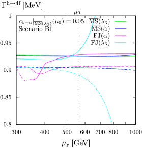
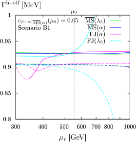
Figure 34: As in Fig. 23, but for scenario B1 with $c_{\beta-\alpha}=0.05$.

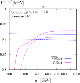
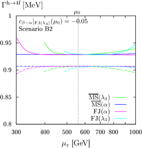
Figure 35: As in Fig. 29, but for scenario B2 with $c_{\beta-\alpha}=-0.05$.

A.2 Differential distributions

For none of the considered benchmark scenarios, we have observed any distortion in the shapes of differential distributions for ${\mathrm{h}}{\to}4f$ decays in the transition from the SM to the THDM. For the low-mass scenarios Aa and Ab this was illustrated in Sec. 4.1.6 for some selected leptonic and semileptonic final states. Here we show the respective distributions for the scenarios B1a and B2b in Figs. 37–39.

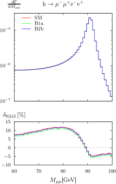
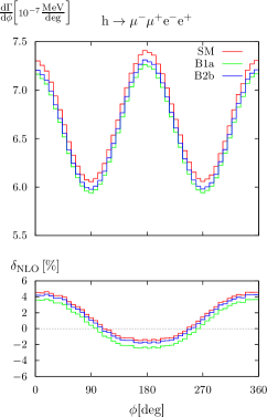
Figure 36: Invariant-mass (a) and angular distributions (b) of the leptonic neutral-current decay $\mathrm{h}\to\mu^{-}\mu^{+}{\mathrm{e}}^{-}{\mathrm{e}}^{+}$ for the SM and the THDM scenarios B1b and B2b. The relative NLO corrections to the distributions are plotted in the lower panels.

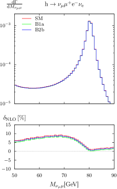
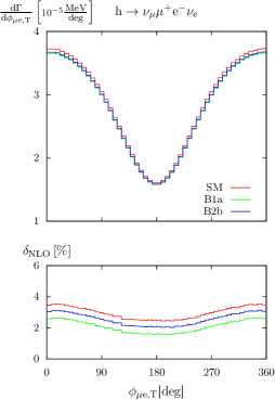
Figure 37: Invariant-mass (a) and angular distributions (b) of the leptonic charged-current decay $\mathrm{h}\to\nu_{\mu}\mu^{+}{\mathrm{e}}^{-}\bar{\nu}_{\mathrm{e}}$ for the SM and the THDM scenarios B1a and B2b. The relative NLO corrections to the distributions are plotted in the lower panels.

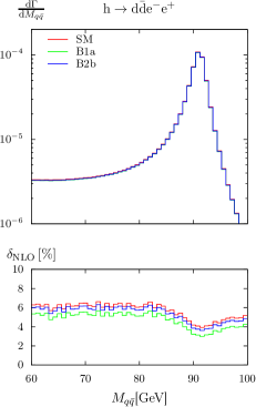
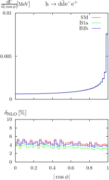
Figure 38: Invariant-mass (a) and angular distributions (b) of the charged-current semi-leptonic decay $\mathrm{h}\to{\mathrm{d}}\bar{{\mathrm{d}}}{\mathrm{e}}^{-}{\mathrm{e}}^{+}$ for the SM and the THDM scenarios B1a and B2b. The relative NLO corrections to the distributions are plotted in the lower panels.

Figure 39: Invariant-mass (a) and angular distributions (b) of the charged-current semi-leptonic decay $\mathrm{h}\to\nu_{\mathrm{e}}{\mathrm{e}}^{+}{\mathrm{d}}\bar{{\mathrm{u}}}$ for the SM and the THDM scenarios B1a and B2b. The relative NLO corrections to the distributions are plotted in the lower panels.

References

- [1] ATLAS Collaboration, G. Aad et al., Observation of a new particle in the search for the Standard Model Higgs boson with the ATLAS detector at the LHC, Phys. Lett. B716 (2012) 1–29, [arXiv:1207.7214].
- [2] CMS Collaboration, S. Chatrchyan et al., Observation of a new boson at a mass of 125 GeV with the CMS experiment at the LHC, Phys.Lett. B716 (2012) 30–61, [arXiv:1207.7235].
- [3] T. D. Lee, A Theory of Spontaneous T Violation, Phys. Rev. D8 (1973) 1226–1239. [,516(1973)].
- [4] J. F. Gunion, H. E. Haber, G. L. Kane, and S. Dawson, The Higgs Hunter’s Guide. Westview, 1900.
- [5] A. Celis, V. Ilisie, and A. Pich, LHC constraints on two-Higgs doublet models, JHEP 07 (2013) 053, [arXiv:1302.4022].
- [6] A. Celis, V. Ilisie, and A. Pich, Towards a general analysis of LHC data within two-Higgs-doublet models, JHEP 12 (2013) 095, [arXiv:1310.7941].
- [7] S. Chang, et al., Two Higgs doublet models for the LHC Higgs boson data at 7 and 8 TeV, JHEP 09 (2014) 101, [arXiv:1310.3374].
- [8] O. Eberhardt, U. Nierste, and M. Wiebusch, Status of the two-Higgs-doublet model of type II, JHEP 07 (2013) 118, [arXiv:1305.1649].
- [9] R. V. Harlander, S. Liebler, and T. Zirke, Higgs Strahlung at the Large Hadron Collider in the 2-Higgs-Doublet Model, JHEP 02 (2014) 023, [arXiv:1307.8122].
- [10] B. Hespel, D. Lopez-Val, and E. Vryonidou, Higgs pair production via gluon fusion in the Two-Higgs-Doublet Model, JHEP 09 (2014) 124, [arXiv:1407.0281].
- [11] J. Baglio, O. Eberhardt, U. Nierste, and M. Wiebusch, Benchmarks for Higgs Pair Production and Heavy Higgs boson Searches in the Two-Higgs-Doublet Model of Type II, Phys. Rev. D90 (2014), no. 1 015008, [arXiv:1403.1264].
- [12] A. Broggio, E. J. Chun, M. Passera, K. M. Patel, and S. K. Vempati, Limiting two-Higgs-doublet models, JHEP 11 (2014) 058, [arXiv:1409.3199].
- [13] H. E. Haber and O. Stål, New LHC benchmarks for the -conserving two-Higgs-doublet model, Eur. Phys. J. C75 (2015), no. 10 491, [arXiv:1507.04281].
- [14] D. Goncalves and D. Lopez-Val, Pseudoscalar searches with dileptonic tops and jet substructure, Phys. Rev. D94 (2016), no. 9 095005, [arXiv:1607.08614].
- [15] G. C. Dorsch, S. J. Huber, K. Mimasu, and J. M. No, Hierarchical versus degenerate 2HDM: The LHC run 1 legacy at the onset of run 2, Phys. Rev. D93 (2016), no. 11 115033, [arXiv:1601.04545].
- [16] G. Cacciapaglia, et al., Search for a lighter Higgs boson in Two Higgs Doublet Models, JHEP 12 (2016) 068, [arXiv:1607.08653].
- [17] V. Cacchio, D. Chowdhury, O. Eberhardt, and C. W. Murphy, Next-to-leading order unitarity fits in Two-Higgs-Doublet models with soft breaking, JHEP 11 (2016) 026, [arXiv:1609.01290].
- [18] R. Aggleton, D. Barducci, N.-E. Bomark, S. Moretti, and C. Shepherd-Themistocleous, Review of LHC experimental results on low mass bosons in multi Higgs models, JHEP 02 (2017) 035, [arXiv:1609.06089].
- [19] X.-F. Han and L. Wang, Two-Higgs-doublet model of type-II confronted with the LHC run-I and run-II data, arXiv:1701.02678.
- [20] D. Bhatia, U. Maitra, and S. Niyogi, Discovery prospects of Light Higgs at LHC in Type-I 2HDM, arXiv:1704.07850.
- [21] A. Arbey, F. Mahmoudi, O. Stal, and T. Stefaniak, Status of the Charged Higgs Boson in Two Higgs Doublet Models, arXiv:1706.07414.
- [22] C. A. Nelson, Correlation Between Decay Planes in Higgs Boson Decays Into Pair (Into Pair), Phys. Rev. D37 (1988) 1220.
- [23] A. Soni and R. M. Xu, Probing CP violation via Higgs decays to four leptons, Phys. Rev. D48 (1993) 5259–5263, [hep-ph/9301225].
- [24] D. Chang, W.-Y. Keung, and I. Phillips, CP odd correlation in the decay of neutral Higgs boson into Z Z, W+ W-, or t anti-t, Phys. Rev. D48 (1993) 3225–3234, [hep-ph/9303226].
- [25] A. Skjold and P. Osland, Angular and energy correlations in Higgs decay, Phys. Lett. B311 (1993) 261–265, [hep-ph/9303294].
- [26] C. P. Buszello, I. Fleck, P. Marquard, and J. J. van der Bij, Prospective analysis of spin- and CP-sensitive variables in at the LHC, Eur. Phys. J. C32 (2004) 209–219, [hep-ph/0212396].
- [27] T. Arens and L. M. Sehgal, Energy spectra and energy correlations in the decay , Z. Phys. C66 (1995) 89–94, [hep-ph/9409396].
- [28] S. Y. Choi, D. J. Miller, M. M. Mühlleitner, and P. M. Zerwas, Identifying the Higgs spin and parity in decays to Z pairs, Phys. Lett. B553 (2003) 61–71, [hep-ph/0210077].
- [29] S. Boselli, et al., Higgs decay into four charged leptons in the presence of dimension-six operators, arXiv:1703.06667.
- [30] A. Bredenstein, A. Denner, S. Dittmaier, and M. M. Weber, Precise predictions for the Higgs-boson decay 4 leptons, Phys. Rev. D74 (2006) 013004, [hep-ph/0604011].
- [31] A. Bredenstein, A. Denner, S. Dittmaier, and M. M. Weber, Precision calculations for the Higgs decays 4 leptons, Nucl. Phys. Proc. Suppl. 160 (2006) 131–135, [hep-ph/0607060].
- [32] A. Bredenstein, A. Denner, S. Dittmaier, and M. M. Weber, Radiative corrections to the semileptonic and hadronic Higgs-boson decays 4 fermions, JHEP 02 (2007) 080, [hep-ph/0611234].
- [33] A. Denner, S. Dittmaier, M. Roth, and D. Wackeroth, Predictions for all processes , Nucl. Phys. B560 (1999) 33–65, [hep-ph/9904472].
- [34] A. Denner, S. Dittmaier, M. Roth, and L. H. Wieders, Electroweak corrections to charged-current processes: Technical details and further results, Nucl. Phys. B724 (2005) 247–294, [hep-ph/0505042]. [Erratum: Nucl. Phys.B854,504(2012)].
- [35] A. Denner and S. Dittmaier, The Complex-mass scheme for perturbative calculations with unstable particles, Nucl. Phys. Proc. Suppl. 160 (2006) 22–26, [hep-ph/0605312].
- [36] S. Boselli, C. M. Carloni Calame, G. Montagna, O. Nicrosini, and F. Piccinini, Higgs boson decay into four leptons at NLOPS electroweak accuracy, JHEP 06 (2015) 023, [arXiv:1503.07394].
- [37] LHC Higgs Cross Section Working Group Collaboration, D. de Florian et al., Handbook of LHC Higgs Cross Sections: 4. Deciphering the Nature of the Higgs Sector, arXiv:1610.07922.
- [38] M. Krause, R. Lorenz, M. Mühlleitner, R. Santos, and H. Ziesche, Gauge-independent Renormalization of the 2-Higgs-Doublet Model, arXiv:1605.04853.
- [39] A. Denner, L. Jenniches, J.-N. Lang, and C. Sturm, Gauge-independent renormalization in the 2HDM, arXiv:1607.07352.
- [40] L. Altenkamp, S. Dittmaier, and H. Rzehak, Renormalization schemes for the Two-Higgs-Doublet Model and applications to , arXiv:1704.02645.
- [41] A. Denner, J.-N. Lang, and S. Uccirati, NLO electroweak corrections in extended Higgs Sectors with RECOLA2, JHEP 07 (2017) 087, [arXiv:1705.06053].
- [42] A. Freitas and D. Stöckinger, Gauge dependence and renormalization of tan beta in the MSSM, Phys. Rev. D66 (2002) 095014, [hep-ph/0205281].
- [43] M. Krause, M. Mühlleitner, R. Santos, and H. Ziesche, 2HDM Higgs-to-Higgs Decays at Next-to-Leading Order, arXiv:1609.04185.
- [44] A. Djouadi, J. Kalinowski, and M. Spira, HDECAY: A Program for Higgs boson decays in the standard model and its supersymmetric extension, Comput. Phys. Commun. 108 (1998) 56–74, [hep-ph/9704448].
- [45] D. Eriksson, J. Rathsman, and O. Stal, 2HDMC: Two-Higgs-Doublet Model Calculator Physics and Manual, Comput. Phys. Commun. 181 (2010) 189–205, [arXiv:0902.0851].
- [46] LHC Higgs Cross Section Working Group Collaboration, J. R. Andersen et al., Handbook of LHC Higgs Cross Sections: 3. Higgs Properties, arXiv:1307.1347.
- [47] R. Harlander, M. Mühlleitner, J. Rathsman, M. Spira, and O. Stål, Interim recommendations for the evaluation of Higgs production cross sections and branching ratios at the LHC in the Two-Higgs-Doublet Model, arXiv:1312.5571.
- [48] A. Denner, S. Dittmaier, and L. Hofer, Collier: a fortran-based Complex One-Loop LIbrary in Extended Regularizations, arXiv:1604.06792.
- [49] S. Berge, S. Groote, J. G. Körner, and L. Kaldamäe, Lepton-mass effects in the decays and , Phys. Rev. D92 (2015), no. 3 033001, [arXiv:1505.06568].
- [50] A. Denner, et al., Higgs Production and Decay with a Fourth Standard-Model-Like Fermion Generation, Eur. Phys. J. C72 (2012) 1992, [arXiv:1111.6395].
- [51] B. W. Harris and J. F. Owens, The Two cutoff phase space slicing method, Phys. Rev. D65 (2002) 094032, [hep-ph/0102128].
- [52] S. Catani and M. H. Seymour, A general algorithm for calculating jet cross sections in NLO QCD, Nucl. Phys. B485 (1997) 291–419, [hep-ph/9605323].
- [53] S. Dittmaier, A General approach to photon radiation off fermions, Nucl. Phys. B565 (2000) 69–122, [hep-ph/9904440].
- [54] S. Dittmaier, A. Kabelschacht, and T. Kasprzik, Polarized QED splittings of massive fermions and dipole subtraction for non-collinear-safe observables, Nucl. Phys. B800 (2008) 146–189, [arXiv:0802.1405].
- [55] LHC Higgs Cross Section Working Group Collaboration, S. Dittmaier et al., Handbook of LHC Higgs Cross Sections: 1. Inclusive Observables, arXiv:1101.0593.
- [56] LHC Higgs Cross Section Working Group Collaboration, S. Dittmaier et al., Handbook of LHC Higgs Cross Sections: 2. Differential Distributions, arXiv:1201.3084.
- [57] J. Fleischer and F. Jegerlehner, Radiative Corrections to Higgs Decays in the Extended Weinberg-Salam Model, Phys. Rev. D23 (1981) 2001–2026.
- [58] S. Actis, A. Ferroglia, M. Passera, and G. Passarino, Two-Loop Renormalization in the Standard Model. Part I: Prolegomena, Nucl. Phys. B777 (2007) 1–34, [hep-ph/0612122].
- [59] T. Hahn, Generating Feynman diagrams and amplitudes with FeynArts 3, Comput. Phys. Commun. 140 (2001) 418–431, [hep-ph/0012260].
- [60] T. Hahn and M. Perez-Victoria, Automatized one-loop calculations in four and D dimensions, Comput. Phys. Commun. 118 (1999) 153–165, [hep-ph/9807565].
- [61] T. Hahn, Automatic loop calculations with FeynArts, FormCalc, and LoopTools, Nucl. Phys. Proc. Suppl. 89 (2000) 231–236, [hep-ph/0005029].
- [62] J. Küblbeck, M. Böhm, and A. Denner, FeynArts: Computer Algebraic Generation of Feynman Graphs and Amplitudes, Comput. Phys. Commun. 60 (1990) 165–180.
- [63] Particle Data Group Collaboration, K. A. Olive et al., Review of Particle Physics, Chin. Phys. C38 (2014) 090001.
- [64] G. C. Dorsch, S. J. Huber, K. Mimasu, and J. M. No, Echoes of the Electroweak Phase Transition: Discovering a second Higgs doublet through , Phys. Rev. Lett. 113 (2014), no. 21 211802, [arXiv:1405.5537].
- [65] G. Cvetic, S. S. Hwang, and C. S. Kim, One loop renormalization group equations of the general framework with two Higgs doublets, Int. J. Mod. Phys. A14 (1999) 769–798, [hep-ph/9706323].
- [66] G. Branco, et al., Theory and phenomenology of two-Higgs-doublet models, Phys.Rept. 516 (2012) 1–102, [arXiv:1106.0034].
- [67] J. Bijnens, J. Lu, and J. Rathsman, Constraining General Two Higgs Doublet Models by the Evolution of Yukawa Couplings, JHEP 05 (2012) 118, [arXiv:1111.5760].
- [68] N. Chakrabarty, U. K. Dey, and B. Mukhopadhyaya, High-scale validity of a two-Higgs doublet scenario: a study including LHC data, JHEP 12 (2014) 166, [arXiv:1407.2145].
- [69] P. Ferreira, H. E. Haber, and E. Santos, Preserving the validity of the Two-Higgs Doublet Model up to the Planck scale, Phys. Rev. D92 (2015) 033003, [arXiv:1505.04001]. [Erratum: Phys. Rev.D94,no.5,059903(2016)].
- [70] T. Kinoshita, Mass singularities of Feynman amplitudes, J. Math. Phys. 3 (1962) 650–677.
- [71] T. D. Lee and M. Nauenberg, Degenerate Systems and Mass Singularities, Phys. Rev. 133 (1964) B1549–B1562.