An $\mathcal{H}_{2}$-Type Error Bound for Time-Limited Balanced Truncation

Abstract

When solving partial differential equations numerically, usually a high order spatial discretization is needed. Model order reduction (MOR) techniques are often used to reduce the order of spatially-discretized systems and hence reduce computational complexity. A particular MOR technique to obtain a reduced order model (ROM) is balanced truncation (BT). However, if one aims at finding a good ROM on a certain finite time interval only, time-limited BT (TLBT) can be a more accurate alternative. So far, no error bound on TLBT has been proved. In this paper, we close this gap in the theory by providing an $\mathcal{H}_{2}$ error bound for TLBT with two different representations. The performance of the error bound is then shown in several numerical experiments.

Keywords: Model reduction; linear systems; time-limited balanced truncation; time-limited Gramians; error bound.

MSC classification: 93A15, 93B99, 93C05, 93C15, 93D20.

1 Introduction

Let $(A,B,C)\in\mathbb{R}^{n\times n}\times\mathbb{R}^{n\times m}\times\mathbb{R}^{p\times m}$ be a realization of a linear, time-invariant system

$$\boldsymbol{\Sigma}:\quad\dot{x}(t)=Ax(t)+Bu(t),\quad x(0)=0,\quad y(t)=Cx(t)$$ (1)

and assume that $A$ is Hurwitz which implies (1) is asymptotically stable. The infinite reachability and observability Gramians

$$P_{\infty}=\int_{0}^{\infty}\operatorname{e}^{As}BB^{T}\operatorname{e}^{A^{T}s}ds,\quad Q_{\infty}=\int_{0}^{\infty}\operatorname{e}^{A^{T}s}C^{T}C\operatorname{e}^{As}ds$$

of $(A,B,C)$ solve the Lyapunov equations

$$AP_{\infty}+P_{\infty}A^{T}+BB^{T}=0,\quad A^{T}Q_{\infty}+Q_{\infty}A^{T}+C^{T}C=0.$$ (2)

The first ingredient of balanced truncation [14] (BT) is to simultaneously diagonalize both Gramians through congruence transformations $\hat{S}P_{\infty}\hat{S}^{T}=\hat{S}^{-T}Q_{\infty}\hat{S}^{-1}=\Sigma_{\infty}$ which gives a balanced realization $(\hat{S}A\hat{S}^{-1},\hat{S}B,C\hat{S}^{-1})$, where $\Sigma_{\infty}$ is diagonal and contains the Hankel singular values $\sigma_{j}$ (HSVs), i.e., the square root of the eigenvalues of $P_{\infty}Q_{\infty}$. In the second step the reduced order model $\boldsymbol{\Sigma}_{r}$ is obtained by keeping only the $r\times r$ upper left block of $\hat{S}A\hat{S}^{-1}$ and the associated parts of $\hat{S}B,C\hat{S}^{-1}$, i.e., the smallest $n-r$ HSVs are removed from the system. With Cholesky factorizations $P_{\infty}=L_{P}L_{P}^{T}$, $Q_{\infty}=L_{Q}L_{Q}^{T}$, and the singular value decomposition (SVD) $X\Sigma_{\infty}Y^{T}=L_{Q}^{T}L_{P}$, the balancing transformation is given by $\hat{S}=L_{Q}X\Sigma_{\infty}^{-\tfrac{1}{2}}$ and $\hat{S}^{-1}=L_{P}Y\Sigma_{\infty}^{-\tfrac{1}{2}}$, see, e.g., [1]. This leads to non increasingly ordered $\sigma_{j}$. Moreover, the resulting reduced system $\boldsymbol{\Sigma}_{r}$ is asymptotically stable and satisfies the $\mathcal{H}_{\infty}$ error bound [9]

$$\|\boldsymbol{\Sigma}-\boldsymbol{\Sigma}_{r}\|_{\mathcal{H}_{\infty}}\leq 2(\sigma_{r+1}+\ldots+\sigma_{n}).$$ (3)

Once the SVD is computed, (3) can be used to adaptively adjust the reduced order $r$. A generalized $\mathcal{H}_{\infty}$-error bound for BT has been proved in [2, 5], where linear stochastic system are investigated.
The matrix of truncated HSVs $\Sigma_{2}=\operatorname{diag}(\sigma_{r+1},\ldots,\sigma_{n})$ can be used to express the $\mathcal{H}_{2}$ error bound [1]. It is represented by

$$\|\boldsymbol{\Sigma}-\boldsymbol{\Sigma}_{r}\|^{2}_{\mathcal{H}_{2}}\leq\operatorname{tr}(\Sigma_{2}(B_{2}B_{2}^{T}+2P_{\infty,M,2}A_{21}^{T})),$$ (4)

where $B_{2}$ is the matrix of the last $n-r$ rows of $\hat{S}B$, $A_{21}$ is the left lower $(n-r)\times r$ block of $\hat{S}A\hat{S}^{-1}$ and $P_{\infty,M,2}$ are the last $n-r$ rows of the mixed Gramian $P_{\infty,M}=\hat{S}\int_{0}^{\infty}\operatorname{e}^{As}BB_{1}^{T}\operatorname{e}^{A_{11}^{T}s}ds$. The bound in (4) has already been extended to stochastic systems in a more general form [3, 7, 15].

In [8] Gawronski and Juang restricted balanced truncation to a finite time interval $[0,\bar{T}]$, $\bar{T}<\infty$, by introducing the time-limited reachability and observability Gramians

$$P_{\bar{T}}:=\int_{0}^{\bar{T}}\operatorname{e}^{As}BB^{T}\operatorname{e}^{A^{T}s}ds,\quad Q_{\bar{T}}=\int_{0}^{\bar{T}}\operatorname{e}^{A^{T}s}C^{T}C\operatorname{e}^{As}ds.$$ (5)

It is easy to show that $P_{\bar{T}},\leavevmode\nobreak\ Q_{\bar{T}}$ solve the Lyapunov equations

$$AP_{\bar{T}}+P_{\bar{T}}A^{T}+BB^{T}-F_{\bar{T}}F_{\bar{T}}^{T} =0,$$ (6)

$$A^{T}Q_{\bar{T}}+Q_{\bar{T}}A^{T}+C^{T}C-G_{\bar{T}}^{T}G_{\bar{T}} =0,$$ (7)

where $G_{t}:=C\operatorname{e}^{At}$ and $F_{t}:=\operatorname{e}^{At}B$, $t\in[0,{\bar{T}}]$. Time-limited balanced truncation (TLBT) is then carried out by using the Cholesky factors of $P_{\bar{T}}$, $Q_{\bar{T}}$ instead of $P_{\infty},Q_{\infty}$ to construct the balancing transformation which in this case is denoted by $S$. This transformation simultaneously diagonalizes $P_{\bar{T}}$, $Q_{\bar{T}}$, i.e., $SP_{\bar{T}}S^{T}=S^{-T}Q_{\bar{T}}S^{-1}=\Sigma_{\bar{T}}$ and is, thus, referred to as time-limited balancing transformation. The values in $\Sigma_{\bar{T}}$ are referred to as time-limited singular values and are, similar to the HSVs, invariant under state-space transformations. Because of the altered Gramian definitions, TLBT does generally not preserve stability and there is no $\mathcal{H}_{\infty}$ error bound as in unrestricted BT.

The main contribution of this paper is a generalized $\mathcal{H}_{2}$ error bound for TLBT. It leads to (4) if $\bar{T}\rightarrow\infty$. We provide two representations of this bound. The first one can be used for practical computations and is, hence, an important tool to assess the obtained accuracy. The second representation is not appropriate for computing the bound but it shows that, similar to BT, the time-limited singular values deliver an alternative criterion to find a suitable reduced order dimension $r$. We conclude this paper by conducting several numerical experiments which indicate that the time-limited $\mathcal{H}_{2}$ bound is tight.

2 $\mathcal{H}_{2}$-type Error Bounds for Time-Limited Balanced Truncation

Let $S$ be the time-limited balancing transformation. We partition the balanced realization $(SAS^{-1},SB,CS^{-1})$ as follows:

$$SAS^{-1}=\begin{bmatrix}{A}_{11}&{A}_{12}\\ {A}_{21}&{A}_{22}\end{bmatrix},\;\;\;SB=\begin{bmatrix}{B}_{1}\\ {B}_{2}\end{bmatrix},\;\;\;CS^{-1}=\begin{bmatrix}{C}_{1}&{C}_{2}\end{bmatrix},$$

where ${A}_{11}\in\mathbb{R}^{r\times r}$, $B_{1}\in\mathbb{R}^{r\times m}$, $C_{1}\in\mathbb{R}^{p\times r}$ and the other blocks of appropriate dimensions. Furthermore, we introduce

$$SF_{\bar{T}}=\begin{bmatrix}F_{{\bar{T}},1}\\ F_{{\bar{T}},2}\end{bmatrix},\;G_{\bar{T}}S^{-1}=\begin{bmatrix}G_{{\bar{T}},1}&G_{{\bar{T}},2}\end{bmatrix},\;\Sigma_{\bar{T}}=\begin{bmatrix}\Sigma_{{\bar{T}},1}&\\ &\Sigma_{{\bar{T}},2}\end{bmatrix}.$$

We consider the corresponding Lyapunov equations in partitioned form:

$$\left[\begin{smallmatrix}{A}_{11}&{A}_{12}\\ {A}_{21}&{A}_{22}\end{smallmatrix}\right]\left[\begin{smallmatrix}\Sigma_{{\bar{T}},1}&\\ &\Sigma_{{\bar{T}},2}\end{smallmatrix}\right]+\left[\begin{smallmatrix}\Sigma_{{\bar{T}},1}&\\ &\Sigma_{{\bar{T}},2}\end{smallmatrix}\right]\left[\begin{smallmatrix}A^{T}_{11}&A^{T}_{21}\\ A^{T}_{12}&A^{T}_{22}\end{smallmatrix}\right]= -\left[\begin{smallmatrix}{B}_{1}B_{1}^{T}&{B}_{1}B_{2}^{T}\\ {B}_{2}B_{1}^{T}&{B}_{2}B_{2}^{T}\end{smallmatrix}\right]$$ (8)

$$+\left[\begin{smallmatrix}F_{\bar{T},1}F_{\bar{T},1}^{T}&F_{\bar{T},1}F_{\bar{T},2}^{T}\\ F_{\bar{T},2}F_{\bar{T},1}^{T}&F_{\bar{T},2}F_{\bar{T},2}^{T}\end{smallmatrix}\right],$$

$$\left[\begin{smallmatrix}{A}^{T}_{11}&{A}^{T}_{21}\\ {A}^{T}_{12}&{A}^{T}_{22}\end{smallmatrix}\right]\left[\begin{smallmatrix}\Sigma_{{\bar{T}},1}&\\ &\Sigma_{{\bar{T}},2}\end{smallmatrix}\right]+\left[\begin{smallmatrix}\Sigma_{{\bar{T}},1}&\\ &\Sigma_{{\bar{T}},2}\end{smallmatrix}\right]\left[\begin{smallmatrix}A_{11}&A_{12}\\ A_{21}&A_{22}\end{smallmatrix}\right]= -\left[\begin{smallmatrix}C_{1}^{T}C_{1}&C_{1}^{T}C_{2}\\ C^{T}_{2}C_{1}&C^{T}_{2}C_{2}\end{smallmatrix}\right]$$ (9)

$$+\left[\begin{smallmatrix}G_{\bar{T},1}^{T}G_{\bar{T},1}&G_{\bar{T},1}^{T}G_{\bar{T},2}\\ G_{\bar{T},2}^{T}G_{\bar{T},1}&G_{\bar{T},2}^{T}G_{\bar{T},2}\end{smallmatrix}\right].$$

The TLBT reduced system that approximates (1) is given by

$$\dot{x}_{r}(t)=A_{11}x_{r}(t)+B_{1}u(t),\quad x_{r}(0)=0,\quad y_{r}(t)=C_{1}x_{r}(t).$$

The goal of this section is to find a bound for the error between $y$ and $y_{r}$. Since we have zero initial conditions for both the reduced and the full system, we have the following representations for the outputs

$$y(t) =Cx(t)=C\int_{0}^{t}\operatorname{e}^{A(t-s)}Bu(s)ds,$$

$$y_{r}(t) =C_{1}x_{r}(t)=C_{1}\int_{0}^{t}\operatorname{e}^{A_{11}(t-s)}B_{1}u(s)ds,$$

where $t\in[0,{\bar{T}}]$. To find a first representation for the error bound, arguments from [3, 7, 15] are used. There a generalized $\mathcal{H}_{2}$ error bound for stochastic systems has been derived. Some easy rearrangements yield a first error estimate

$$\left\|y(t)-y_{r}(t)\right\|_{2}$$

$$=\left\|C\int_{0}^{t}\operatorname{e}^{A(t-s)}Bu(s)ds-C_{1}\int_{0}^{t}\operatorname{e}^{A_{11}(t-s)}B_{1}u(s)ds\right\|_{2}$$

$$\leq\int_{0}^{t}\left\|\left(C\operatorname{e}^{A(t-s)}B-C_{1}\operatorname{e}^{A_{11}(t-s)}B_{1}\right)u(s)\right\|_{2}ds$$

$$\leq\int_{0}^{t}\left\|C\operatorname{e}^{A(t-s)}B-C_{1}\operatorname{e}^{A_{11}(t-s)}B_{1}\right\|_{F}\left\|u(s)\right\|_{2}ds.$$

By the Cauchy Schwarz inequality it holds that

$$\left\|y(t)-y_{r}(t)\right\|_{2}$$

$$\leq\left(\int_{0}^{t}\left\|C\operatorname{e}^{A(t-s)}B-C_{1}\operatorname{e}^{A_{11}(t-s)}B_{1}\right\|_{F}^{2}ds\right)^{\frac{1}{2}}\left(\int_{0}^{t}\left\|u(s)\right\|_{2}^{2}ds\right)^{\frac{1}{2}}.$$

Using substitution, the definition of the Frobenius norm and the linearity of the integral, we obtain

$$\int_{0}^{t}\left\|C\operatorname{e}^{A(t-s)}B-C_{1}\operatorname{e}^{A_{11}(t-s)}B_{1}\right\|_{F}^{2}ds$$

$$=\int_{0}^{t}\left\|C\operatorname{e}^{As}B-C_{1}\operatorname{e}^{A_{11}s}B_{1}\right\|_{F}^{2}ds$$

$$\leq\int_{0}^{\bar{T}}\left\|C\operatorname{e}^{As}B-C_{1}\operatorname{e}^{A_{11}s}B_{1}\right\|_{F}^{2}ds$$

$$=\int_{0}^{\bar{T}}\operatorname{tr}\left(C\operatorname{e}^{As}BB^{T}\operatorname{e}^{A^{T}s}C^{T}\right)ds$$

$$\quad+\int_{0}^{\bar{T}}\operatorname{tr}\left(C_{1}\operatorname{e}^{A_{11}s}B_{1}B_{1}^{T}\operatorname{e}^{A_{11}^{T}s}C_{1}^{T}\right)ds$$

$$\quad-2\int_{0}^{\bar{T}}\operatorname{tr}\left(C\operatorname{e}^{As}BB_{1}^{T}\operatorname{e}^{A_{11}^{T}s}C_{1}^{T}\right)ds$$

$$=\operatorname{tr}\left(CP_{\bar{T}}C^{T}\right)+\operatorname{tr}\left(C_{1}P_{{\bar{T}},r}C_{1}^{T}\right)-2\;\operatorname{tr}\left(CP_{{\bar{T}},M}C_{1}^{T}\right),$$

where $P_{\bar{T}}:=\int_{0}^{\bar{T}}\operatorname{e}^{As}BB^{T}\operatorname{e}^{A^{T}s}ds$, $P_{{\bar{T}},r}:=\int_{0}^{\bar{T}}\operatorname{e}^{A_{11}s}B_{1}B_{1}^{T}\operatorname{e}^{A_{11}^{T}s}ds$ and $P_{{\bar{T}},M}:=\int_{0}^{\bar{T}}\operatorname{e}^{As}BB_{1}^{T}\operatorname{e}^{A_{11}^{T}s}ds$. Matrix-valued integrals of this form can under some conditions be expressed as unique solutions of matrix equations.

Lemma 2.1.

Let $A_{1}\in\mathbb{R}^{n\times n},\leavevmode\nobreak\ A_{2}\in\mathbb{R}^{r\times r}$ with $\Lambda(A_{1})\cap-\Lambda(A_{2})=\emptyset$ and $B_{1}\in\mathbb{R}^{n\times m}$, $B_{2}\in\mathbb{R}^{r\times m}$. Then,

$$X=\int_{0}^{\bar{T}}\operatorname{e}^{A_{1}s}B_{1}B_{2}^{T}\operatorname{e}^{A_{2}^{T}s}ds$$

solves the Sylvester equation

$$A_{1}X+XA_{2}^{T} =-B_{1}B_{2}^{T}+\operatorname{e}^{A_{1}{\bar{T}}}B_{1}B_{2}^{T}\operatorname{e}^{A_{2}^{T}{\bar{T}}}.$$

Proof.

The integral is equivalent to

$$\operatorname{vec}X =\int_{0}^{\bar{T}}\operatorname{vec}\operatorname{e}^{A_{1}s}B_{1}B_{2}^{T}\operatorname{e}^{A_{2}^{T}s}ds$$

$$=\int_{0}^{\bar{T}}\operatorname{e}^{A_{2}s}\otimes\operatorname{e}^{A_{1}s}ds\operatorname{vec}B_{1}B_{2}^{T}$$

$$=\int_{0}^{\bar{T}}\operatorname{e}^{\left(I_{r}\otimes A_{1}+A_{2}\otimes I_{n}\right)s}ds\operatorname{vec}B_{1}B_{2}^{T},$$

where we used [12, Theorem 10.9]. The matrix $\mathcal{A}:=I_{r}\otimes A_{1}+A_{2}\otimes I_{n}$ is nonsingular and it holds that

$$\operatorname{vec}X =\mathcal{A}^{-1}\left(\operatorname{e}^{\mathcal{A}{\bar{T}}}-I_{nr}\right)\operatorname{vec}B_{1}B_{2}^{T}$$

$$\Leftrightarrow\quad\mathcal{A}\operatorname{vec}X =\left(\operatorname{e}^{\mathcal{A}{\bar{T}}}-I_{nr}\right)\operatorname{vec}B_{1}B_{2}^{T}$$

and the claim follows after de-vectorization. ∎

Remark.

The result of the above Lemma is also a consequence of the product rule. Setting $g_{1}(t):=\operatorname{e}^{A_{1}t}B_{1}$ and $g_{2}(t):=B_{2}^{T}\operatorname{e}^{A_{2}^{T}t}$, it holds that

$$g_{1}(\bar{T})g_{2}(\bar{T})-g_{1}(0)g_{2}(0)=\int_{0}^{\bar{T}}g_{1}(s)dg_{2}(s)+\int_{0}^{\bar{T}}dg_{1}(s)g_{2}(s)$$

$$=\int_{0}^{\bar{T}}g_{1}(s)g_{2}(s)ds\;A_{2}^{T}+A_{1}\int_{0}^{\bar{T}}g_{1}(s)g_{2}(s)ds,$$

since $dg_{2}(s)=g_{2}(s)A_{2}^{T}ds$ and $dg_{1}(s)=A_{1}g_{1}(s)ds$.

The time-limited Gramians (5) also exists for unstable systems. Therefore, it is, e.g. in [1, Section 7.6.5], discussed to use TLBT to reduce unstable systems. The above Lemma further reveals that in this situation and if $\Lambda(A)\cap-\Lambda(A)=\emptyset$, the time-limited Gramians can still be obtained by solving the time-limited Lyapunov equations (6) which is important from a numerical point of view. In this work, however, we will not pursue the reduction of unstable systems further.

From now on we assume that $\Lambda(A_{11})\cap-\Lambda(A_{11})=\emptyset$ and $\Lambda(A)\cap-\Lambda(A_{11})=\emptyset$, implying by Lemma 2.1 that the matrices $P_{{\bar{T}},r}$ and $P_{{\bar{T}},M}$ are the unique solutions of

$$A_{11}P_{{\bar{T}},r}+P_{{\bar{T}},r}A_{11}^{T} =-B_{1}B_{1}^{T}+F_{{\bar{T}},r}F_{{\bar{T}},r}^{T},$$ (10a)

$$AP_{{\bar{T}},M}+P_{{\bar{T}},M}A_{11}^{T} =-BB_{1}^{T}+F_{{\bar{T}}}F_{{\bar{T}},r}^{T},$$ (10b)

where $F_{{\bar{T}},r}:=\operatorname{e}^{A_{11}T}B_{1}$. We have, thus, established the following result.

Theorem 2.2.

Let $\Lambda(A_{11})\cap-\Lambda(A_{11})=\emptyset$ and $\Lambda(A)\cap-\Lambda(A_{11})=\emptyset$. Then the following error bound holds for the reduced system $\boldsymbol{\Sigma}_{r}$ generated by TLBT

$$\begin{split}&\max_{t\in[0,{\bar{T}}]}\left\|y(t)-y_{r}(t)\right\|_{2}\leq\epsilon\left\|u\right\|_{L^{2}_{\bar{T}}},\\ &\epsilon:=\left(\operatorname{tr}\left(CP_{\bar{T}}C^{T}\right)+\operatorname{tr}\left(C_{1}P_{{\bar{T}},r}C_{1}^{T}\right)-2\operatorname{tr}\left(CP_{{\bar{T}},M}C_{1}^{T}\right)\right)^{\frac{1}{2}}.\end{split}$$ (11)

The representation (11) of the error bound has the same structure as the one computed in the stochastic framework [3, 7, 15] but it is clearly different since solutions of different matrix equations enter in the time-limited case. The bound in (11) can be used for practical computations. It only requires to solve the matrix equations in (10) since $P_{\bar{T}}$ is already known from the balancing procedure. The matrix equations (10) are not expensive since $P_{{\bar{T}},r}$ usually is a small matrix and $P_{{\bar{T}},M}$ only has a few columns.

The next theorem provides an alternative representation of this bound. It can be expressed with the help of $\Sigma_{{\bar{T}},2}=\operatorname{diag}(\sigma_{{\bar{T}},r+1},\ldots,\sigma_{{\bar{T}},n})$ which is the matrix of truncated time-limited singular values. In [3, 7, 15] representations of generalized $\mathcal{H}_{2}$ error bounds have been shown using the truncated HSVs of the underlying stochastic system. However, the matrix equations (6) and (10) have a very different structure than the generalized equations for stochastic system. Therefore, we need to apply other techniques in order to obtain the result below. This result also shows essential differences in its structure compared to the stochastic case.

Theorem 2.3.

Using the coefficients of the balanced realization of the system, the error bound in (11) can be expressed as follows:

$$\operatorname{tr}\left(CP_{\bar{T}}C^{T}+C_{1}P_{{\bar{T}},r}C_{1}^{T}-2CP_{{\bar{T}},M}C_{1}^{T}\right)$$

$$= \operatorname{tr}(\Sigma_{{\bar{T}},2}(B_{2}B_{2}^{T}+2P_{{\bar{T}},M,2}A_{21}^{T}))-2\operatorname{tr}(G^{T}_{{\bar{T}},1}G_{\bar{T}}P_{{\bar{T}},M})$$

$$+\operatorname{tr}(G^{T}_{{\bar{T}},1}G_{{\bar{T}},1}P_{{\bar{T}},r})+\operatorname{tr}(F_{{\bar{T}},1}F^{T}_{{\bar{T}},1}\Sigma_{{\bar{T}},1})$$

$$-\operatorname{tr}((F_{{\bar{T}},1}-F_{{\bar{T}},r})(F_{{\bar{T}},1}-F_{{\bar{T}},r})^{T}\Sigma_{{\bar{T}},1}),$$

where $P_{{\bar{T}},M,2}$ are the last $n-r$ rows of $SP_{{\bar{T}},M}$ with $S$ being the balancing transformation.

Proof.

By selecting the left and right upper block of (9), we have

$$A_{11}^{T}\Sigma_{{\bar{T}},1}+\Sigma_{{\bar{T}},1}A_{11} =-C_{1}^{T}C_{1}+G_{{\bar{T}},1}^{T}G_{{\bar{T}},1}$$ (12)

$$A_{21}^{T}\Sigma_{{\bar{T}},2}+\Sigma_{{\bar{T}},1}A_{12} =-C_{1}^{T}C_{2}+G_{{\bar{T}},1}^{T}G_{{\bar{T}},2}.$$ (13)

We introduce the reduced order system observability Gramian $Q_{{\bar{T}},r}:=\int_{0}^{\bar{T}}\operatorname{e}^{A^{T}_{11}s}C_{1}^{T}C_{1}\operatorname{e}^{A_{11}s}ds$ which satisfies

$$A_{11}^{T}Q_{{\bar{T}},r}+Q_{{\bar{T}},r}A_{11}=-C_{1}^{T}C_{1}+G_{{\bar{T}},r}^{T}G_{{\bar{T}},r}$$ (14)

with $G_{{\bar{T}},r}:=C_{1}\operatorname{e}^{A_{11}{\bar{T}}}$. We make use of the integral representations of $P_{\bar{T}}$ and $Q_{\bar{T}}$ and apply properties of the trace. Hence, we have

$$\operatorname{tr}(CP_{\bar{T}}C^{T})=\int_{0}^{\bar{T}}\operatorname{tr}(C\operatorname{e}^{As}BB^{T}\operatorname{e}^{A^{T}s}C^{T})ds$$

$$=\int_{0}^{\bar{T}}\operatorname{tr}(B^{T}\operatorname{e}^{A^{T}s}C^{T}C\operatorname{e}^{As}B)ds=\operatorname{tr}(B^{T}Q_{\bar{T}}B).$$

Using the balancing transformation $S$ and the partition of $SB$, we obtain

$$\operatorname{tr}(B^{T}Q_{\bar{T}}B) =\operatorname{tr}(B^{T}S^{T}S^{-T}Q_{\bar{T}}S^{-1}SB)=\operatorname{tr}(B^{T}S^{T}\Sigma_{\bar{T}}SB)$$

$$=\operatorname{tr}(B_{1}^{T}\Sigma_{\bar{T},1}B_{1})+\operatorname{tr}(B_{2}^{T}\Sigma_{\bar{T},2}B_{2}).$$

The partition of $CS^{-1}$ and $SP_{{\bar{T}},M}=\left[\begin{smallmatrix}P_{{\bar{T}},M,1}\\ P_{{\bar{T}},M,2}\end{smallmatrix}\right]$ yield

$$\operatorname{tr}(CP_{\bar{T},M}C_{1}^{T}) =\operatorname{tr}(CS^{-1}SP_{\bar{T},M}C_{1}^{T})$$

$$=\operatorname{tr}(C_{1}P_{\bar{T},M,1}C_{1}^{T})+\operatorname{tr}(C_{2}P_{\bar{T},M,2}C_{1}^{T}).$$

For $\epsilon$ in (11) this leads to

$$\epsilon^{2}= \operatorname{tr}(B_{1}^{T}\Sigma_{{\bar{T}},1}B_{1})+\operatorname{tr}(B_{2}^{T}\Sigma_{{\bar{T}},2}B_{2})+\operatorname{tr}(C_{1}P_{{\bar{T}},r}C_{1}^{T})$$ (15)

$$-2\operatorname{tr}(C_{1}P_{{\bar{T}},M,1}C_{1}^{T})-2\operatorname{tr}(C_{2}P_{{\bar{T}},M,2}C_{1}^{T}).$$

We insert equation (13) which yields

$$\operatorname{tr}(C_{2}P_{{\bar{T}},M,2}C_{1}^{T}) =\operatorname{tr}(P_{{\bar{T}},M,2}C_{1}^{T}C_{2})$$

$$=-\operatorname{tr}(P_{{\bar{T}},M,2}(A_{21}^{T}\Sigma_{{\bar{T}},2}+\Sigma_{{\bar{T}},1}A_{12}))$$

$$\quad+\operatorname{tr}(P_{{\bar{T}},M,2}G_{{\bar{T}},1}^{T}G_{{\bar{T}},2})$$

$$=-\operatorname{tr}(\Sigma_{{\bar{T}},2}P_{{\bar{T}},M,2}A_{21}^{T})-\operatorname{tr}(\Sigma_{{\bar{T}},1}A_{12}P_{{\bar{T}},M,2})$$

$$\quad+\operatorname{tr}(G_{{\bar{T}},1}^{T}G_{{\bar{T}},2}P_{{\bar{T}},M,2}).$$

We multiply (10b) with $S$ from the left and evaluate the resulting upper block of the equation:

$$-A_{12}P_{{\bar{T}},M,2}=A_{11}P_{{\bar{T}},M,1}+P_{{\bar{T}},M,1}A_{11}^{T}+B_{1}B_{1}^{T}-F_{{\bar{T}},1}F_{{\bar{T}},r}^{T}.$$

Hence, we have

$$-2\operatorname{tr}(C_{2}P_{{\bar{T}},M,2}C_{1}^{T})=$$

$$2[\operatorname{tr}(\Sigma_{{\bar{T}},1}F_{{\bar{T}},1}F_{{\bar{T}},r}^{T})-\operatorname{tr}(\Sigma_{{\bar{T}},1}(B_{1}B_{1}^{T}+A_{11}P_{{\bar{T}},M,1}+P_{{\bar{T}},M,1}A_{11}^{T}))]$$

$$+2[\operatorname{tr}(\Sigma_{2}P_{{\bar{T}},M,2}A_{21}^{T})-\operatorname{tr}(G_{{\bar{T}},1}^{T}G_{{\bar{T}},2}P_{{\bar{T}},M,2})].$$

Using equation (12), we obtain

$$\operatorname{tr}(\Sigma_{{\bar{T}},1}(A_{11}P_{{\bar{T}},M,1}+P_{{\bar{T}},M,1}A_{11}^{T})) =\operatorname{tr}(P_{{\bar{T}},M,1}(\Sigma_{{\bar{T}},1}A_{11}+A_{11}^{T}\Sigma_{{\bar{T}},1}))$$

$$=\operatorname{tr}(P_{{\bar{T}},M,1}(G_{{\bar{T}},1}^{T}G_{{\bar{T}},1}-C_{1}^{T}C_{1})),$$

so that

$$-2\operatorname{tr}(C_{2}P_{{\bar{T}},M,2}C_{1}^{T})$$

$$=2[\operatorname{tr}(\Sigma_{{\bar{T}},2}P_{{\bar{T}},M,2}A_{21}^{T})-\operatorname{tr}(B_{1}^{T}\Sigma_{{\bar{T}},1}B_{1})+\operatorname{tr}(C_{1}P_{{\bar{T}},M,1}C_{1}^{T})]$$

$$\quad+2[\operatorname{tr}(\Sigma_{{\bar{T}},1}F_{{\bar{T}},1}F_{{\bar{T}},r}^{T})-\operatorname{tr}(G_{{\bar{T}},1}^{T}G_{{\bar{T}}}P_{{\bar{T}},M})].$$

Inserting this result into equation (15) provides

$$\epsilon^{2}= \operatorname{tr}(\Sigma_{{\bar{T}},2}(B_{2}B_{2}^{T}+2P_{{\bar{T}},M,2}A_{21}^{T}))$$

$$+2[\operatorname{tr}(\Sigma_{{\bar{T}},1}F_{{\bar{T}},1}F_{{\bar{T}},r}^{T})-\operatorname{tr}(G_{{\bar{T}},1}^{T}G_{{\bar{T}}}P_{{\bar{T}},M})]$$

$$+\operatorname{tr}(C_{1}P_{{\bar{T}},r}C_{1}^{T})-\operatorname{tr}(B_{1}^{T}\Sigma_{{\bar{T}},1}B_{1}).$$

With the integral representations of $P_{{\bar{T}},r}$ and $Q_{{\bar{T}},r}$ it holds that

$$\operatorname{tr}(C_{1}P_{{\bar{T}},r}C_{1}^{T})=\int_{0}^{\bar{T}}\operatorname{tr}(C_{1}\operatorname{e}^{A_{11}s}B_{1}B_{1}^{T}\operatorname{e}^{A_{11}^{T}s}C_{1}^{T})ds$$

$$=\int_{0}^{\bar{T}}\operatorname{tr}(B_{1}^{T}\operatorname{e}^{A_{11}^{T}s}C_{1}^{T}C_{1}\operatorname{e}^{A_{11}s}B_{1})ds=\operatorname{tr}(B_{1}^{T}Q_{{\bar{T}},r}B_{1}).$$

So, we have

$$\operatorname{tr}(C_{1}P_{{\bar{T}},r}C_{1}^{T})-\operatorname{tr}(B_{1}^{T}\Sigma_{{\bar{T}},1}B_{1})=\operatorname{tr}(B_{1}B_{1}^{T}(Q_{{\bar{T}},r}-\Sigma_{{\bar{T}},1})).$$

Combining equations (12) and (14), we have

$$A_{11}^{T}(Q_{{\bar{T}},r}-\Sigma_{{\bar{T}},1})+(Q_{{\bar{T}},r}-\Sigma_{{\bar{T}},1})A_{11}=G_{{\bar{T}},r}^{T}G_{{\bar{T}},r}-G_{{\bar{T}},1}^{T}G_{{\bar{T}},1}.$$ (16)

Inserting (10a) and (16) gives

$$\operatorname{tr}(C_{1}P_{{\bar{T}},r}C_{1}^{T})-\operatorname{tr}(B_{1}^{T}\Sigma_{{\bar{T}},1}B_{1})$$

$$=-\operatorname{tr}((A_{11}P_{{\bar{T}},r}+P_{{\bar{T}},r}A_{11}^{T}-F_{{\bar{T}},r}F_{{\bar{T}},r}^{T})(Q_{{\bar{T}},r}-\Sigma_{{\bar{T}},1}))$$

$$=-\operatorname{tr}(P_{{\bar{T}},r}((Q_{{\bar{T}},r}-\Sigma_{{\bar{T}},1})A_{11}+A_{11}^{T}(Q_{{\bar{T}},r}-\Sigma_{{\bar{T}},1})))$$

$$\quad+\operatorname{tr}(F_{{\bar{T}},r}F_{{\bar{T}},r}^{T}(Q_{{\bar{T}},r}-\Sigma_{{\bar{T}},1}))$$

$$=\operatorname{tr}(P_{{\bar{T}},r}(G_{{\bar{T}},1}^{T}G_{{\bar{T}},1}-G_{{\bar{T}},r}^{T}G_{{\bar{T}},r}))+\operatorname{tr}(F_{{\bar{T}},r}F_{{\bar{T}},r}^{T}(Q_{{\bar{T}},r}-\Sigma_{{\bar{T}},1})).$$

Using again the integral representations of $P_{{\bar{T}},r}$ and $Q_{{\bar{T}},r}$, we see that

$$\operatorname{tr}(P_{{\bar{T}},r}G_{{\bar{T}},r}^{T}G_{{\bar{T}},r}) =\int_{0}^{\bar{T}}\operatorname{tr}(\operatorname{e}^{A_{11}s}B_{1}B_{1}^{T}\operatorname{e}^{A_{11}^{T}s}\operatorname{e}^{A^{T}_{11}{\bar{T}}}C_{1}C_{1}^{T}\operatorname{e}^{A_{11}{\bar{T}}})ds$$

$$=\int_{0}^{\bar{T}}\operatorname{tr}(C_{1}^{T}\operatorname{e}^{A_{11}s}\operatorname{e}^{A_{11}{\bar{T}}}B_{1}B_{1}^{T}\operatorname{e}^{A^{T}_{11}{\bar{T}}}\operatorname{e}^{A_{11}^{T}s}C_{1})ds$$

$$=\int_{0}^{\bar{T}}\operatorname{tr}(B_{1}^{T}\operatorname{e}^{A^{T}_{11}{\bar{T}}}\operatorname{e}^{A_{11}^{T}s}C_{1}C_{1}^{T}\operatorname{e}^{A_{11}s}\operatorname{e}^{A_{11}{\bar{T}}}B_{1})ds$$

$$=\operatorname{tr}(F_{{\bar{T}},r}^{T}Q_{{\bar{T}},r}F_{{\bar{T}},r})=\operatorname{tr}(F_{{\bar{T}},r}F_{{\bar{T}},r}^{T}Q_{{\bar{T}},r}).$$

Hence, we have

$$\operatorname{tr}(C_{1}P_{{\bar{T}},r}C_{1}^{T})-\operatorname{tr}(B_{1}^{T}\Sigma_{{\bar{T}},1}B_{1})=\operatorname{tr}(P_{{\bar{T}},r}G_{{\bar{T}},1}^{T}G_{{\bar{T}},1})-\operatorname{tr}(F_{{\bar{T}},r}F_{{\bar{T}},r}^{T}\Sigma_{{\bar{T}},1}).$$

The error bound $\epsilon^{2}$ then is

$$\epsilon^{2}= \operatorname{tr}(\Sigma_{{\bar{T}},2}(B_{2}B_{2}^{T}+2P_{{\bar{T}},M,2}A_{21}^{T}))$$

$$+2[\operatorname{tr}(\Sigma_{{\bar{T}},1}F_{{\bar{T}},1}F_{{\bar{T}},r}^{T})-\operatorname{tr}(G_{{\bar{T}},1}^{T}G_{{\bar{T}}}P_{{\bar{T}},M})]$$

$$+\operatorname{tr}(P_{{\bar{T}},r}G_{{\bar{T}},1}^{T}G_{{\bar{T}},1})-\operatorname{tr}(F_{{\bar{T}},r}F_{{\bar{T}},r}^{T}\Sigma_{{\bar{T}},1}).$$

Since

$$2\operatorname{tr}(\Sigma_{{\bar{T}},1}F_{{\bar{T}},1}F_{{\bar{T}},r}^{T})=2\left\langle\Sigma_{{\bar{T}},1}^{\frac{1}{2}}F_{{\bar{T}},r},\Sigma_{{\bar{T}},1}^{\frac{1}{2}}F_{{\bar{T}},1}\right\rangle_{F}$$

$$= \left\|\Sigma_{{\bar{T}},1}^{\frac{1}{2}}F_{{\bar{T}},r}\right\|^{2}_{F}+\left\|\Sigma_{{\bar{T}},1}^{\frac{1}{2}}F_{{\bar{T}},1}\right\|^{2}_{F}-\left\|\Sigma_{{\bar{T}},1}^{\frac{1}{2}}(F_{{\bar{T}},1}-F_{{\bar{T}},r})\right\|^{2}_{F},$$

we obtain

$$\epsilon^{2}= \operatorname{tr}(\Sigma_{{\bar{T}},2}(B_{2}B_{2}^{T}+2P_{{\bar{T}},M,2}A_{21}^{T}))$$

$$+\operatorname{tr}(\Sigma_{{\bar{T}},1}F_{{\bar{T}},1}F_{{\bar{T}},1}^{T}))-2\operatorname{tr}(P_{{\bar{T}},M}G_{{\bar{T}},1}^{T}G_{{\bar{T}}})+\operatorname{tr}(P_{{\bar{T}},r}G_{{\bar{T}},1}^{T}G_{{\bar{T}},1})$$

$$-\operatorname{tr}(\Sigma_{{\bar{T}},1}(F_{{\bar{T}},1}-F_{{\bar{T}},r})(F_{{\bar{T}},1}-F_{{\bar{T}},r})^{T})$$

which is the claimed result. ∎

We now discuss the impact of the remainder term $R_{\bar{T}}:=-2\operatorname{tr}(G^{T}_{{\bar{T}},1}G_{\bar{T}}P_{{\bar{T}},M})+\operatorname{tr}(G^{T}_{{\bar{T}},1}G_{{\bar{T}},1}P_{{\bar{T}},r})+\operatorname{tr}(F_{{\bar{T}},1}F^{T}_{{\bar{T}},1}\Sigma_{{\bar{T}},1})$ of the error bound in Theorem 2.3. Every summand of $R_{\bar{T}}$ can be bounded from above as follows:

$$\operatorname{tr}(G^{T}_{{\bar{T}},1}G_{\bar{T}}P_{{\bar{T}},M}) \leq\left\|G_{{\bar{T}},1}\right\|_{F}\left\|G_{{\bar{T}}}\right\|_{F}\left\|P_{{\bar{T}},M}\right\|_{F},$$

$$\operatorname{tr}(F_{{\bar{T}},1}F^{T}_{{\bar{T}},1}\Sigma_{{\bar{T}},1}) =\left\|\Sigma_{{\bar{T}},1}^{\frac{1}{2}}F_{{\bar{T}},1}\right\|^{2}_{F}\leq\left\|F_{{\bar{T}},1}\right\|^{2}_{F}\operatorname{tr}(\Sigma_{{\bar{T}},1}),$$

$$\operatorname{tr}(G^{T}_{{\bar{T}},1}G_{{\bar{T}},1}P_{{\bar{T}},r}) =\left\|P_{{\bar{T}},r}^{\frac{1}{2}}G^{T}_{{\bar{T}},1}\right\|^{2}_{F}\leq\left\|G_{{\bar{T}},1}\right\|^{2}_{F}\operatorname{tr}(P_{{\bar{T}},r}).$$

If $A$ is asymptotically stable, then the norms $\left\|F_{{\bar{T}},1}\right\|_{F}$,$\left\|G_{{\bar{T}},1}\right\|_{F}$ and $\left\|G_{{\bar{T}}}\right\|_{F}$ decay exponentially fast, i.e., they are bounded by $c_{1}\operatorname{e}^{-c_{2}{\bar{T}}}$, where $c_{1},c_{2}>0$ are suitable constants.

Now, if the terminal time $\bar{T}$ is sufficiently large, the term $R_{\bar{T}}$ is small and hence it can be neglected in the error bound. For very stable systems ($c_{2}$ is large), $\bar{T}$ can be chosen small and for slowly decaying systems (small constant $c_{2}$), $\bar{T}$ needs to be large in order to have a sufficiently small $R_{\bar{T}}$. If the remainder term $R_{\bar{T}}$ is small, it can be concluded from Theorem 2.3 that TLBT works well if the truncated time-limited singular values $\sigma_{{\bar{T}},r+1},\ldots,\sigma_{{\bar{T}},n}$ are small.

For non-stable systems the remainder term $R_{\bar{T}}$ in the error bound is expected to be large (exponential growth) which might be an indicator for a large error when applying TLBT to these systems.

Remark.

The representation in Theorem 2.3 is not appropriate to determine the error bound since $B_{2}$ and $A_{21}$ are never computed in practice. However, for asymptotically stable systems (1) ($R_{\bar{T}}$ is expected to be small) we know that the reduced order dimension $r$ has to be chosen such that $\sigma_{{\bar{T}},r+1},\ldots,\sigma_{{\bar{T}},n}$ are small in order to guarantee a good approximation. Consequently, looking at the time-limited singular values instead of computing the error bound (11) provides an alternative way to find a suitable reduced order dimension.

3 Practical Considerations

Here we review the practical execution of TLBT for large-scale systems and evaluate the usefulness of the error bound (11) in actual computations. Directly solving the Lyapunov equations (2), (6) is infeasible for large dimensions. Therefore, for large-scale systems it has become common practice to approximate the Gramians by low-rank factorizations, e.g., $P_{\infty}\approx Z_{\infty}Z_{\infty}^{T}$ with low-rank factors $Z_{\infty}\in\mathbb{R}^{n\times h}$, rank$(Z_{\infty})=h\ll n$, and similarly for the other Gramians. This is justified by the often observed and proven fast singular value decay of solutions of Lyapunov equations [11], especially if $p,m\ll n$. For this situation there exist efficient algorithms [4, 16] employing techniques from sparse numerical linear algebra for computing the low-rank solution factors. For the Lyapunov equations (6) in TLBT, a rational Krylov subspace method [6] is proposed in [13] that is also able to deal with the arising matrix exponentials. With low-rank approximations $P_{\bar{T}}\approx Z_{P_{\bar{T}}}Z_{P_{\bar{T}}}^{T}$, $Q_{\bar{T}}\approx Z_{Q_{\bar{T}}}Z_{Q_{\bar{T}}}^{T}$, one computes the SVD $X\Sigma Y^{T}=Z_{P_{\bar{T}}}^{T}Z_{Q_{\bar{T}}}$ and projection matrices $V=Z_{P_{\bar{T}}}Y_{1}\Sigma_{1}^{-\tfrac{1}{2}}$ and $W:=Z_{Q_{\bar{T}}}X_{1}\Sigma_{1}^{-\tfrac{1}{2}}$, where $\Sigma_{1}$ contains the largest $r$ singular values and $X_{1},Y_{1}$ the associated singular vectors. The reduced order model $\boldsymbol{\Sigma}_{r}$ is obtained via $A_{11}:=W^{T}AV$, $B_{1}:=W^{T}B$, $C_{1}:=CV$ which makes it clear that some of the quantities of the bound in Theorem 2.3 are not accessible in practical computations.

However, we may nevertheless acquire an approximation of (11). For this $\operatorname{tr}\left(CP_{\bar{T}}C^{T}\right)$ can be approximated by $\operatorname{tr}\left(CZ_{P_{\bar{T}}}^{T}Z_{P_{\bar{T}}}C^{T}\right)$, $\operatorname{tr}\left(C_{1}P_{\bar{T},r}C_{1}^{T}\right)$ requires solving the $r$ dimensional Lyapunov equation (10a), and $\operatorname{tr}\left(CP_{\bar{T},M}C_{1}^{T}\right)$ requires the solution of the Sylvester equation (10b), which amounts to solve $r$ linear systems of equations defined by $A-\alpha I$, $\alpha\in\Lambda(A_{11})$ see, e.g., [10, Algorithm 7.6.2]. Unlike the error bound in BT (3), the TLBT bound (11) cannot be easily used to adjust the reduced order because when changing $r$ to, say, $r+d$, $d\geq 1$, the solutions of (10) have to be computed entirely from scratch. Especially because of the Sylvester equation (10b), this would be increasingly expensive.

TLBT can with minor adjustments be applied to generalized state-space systems

$$\boldsymbol{\Sigma}:\quad E\dot{x}(t)=Ax(t)+Bu(t),\quad x(0)=0,\quad y(t)=Cx(t)$$ (17)

with $E$ nonsingular. In that case the time-limited Gramians are $P_{\bar{T}}$, $E^{T}Q_{\bar{T}}E$, where $P_{\bar{T}}$, $Q_{\bar{T}}$ solve the generalized Lyapunov equations

$$\begin{split}AP_{\bar{T}}E^{T}+EP_{\bar{T}}A^{T}+BB^{T}-F^{E}_{\bar{T}}(F^{E}_{\bar{T}})^{T}&=0,\\ A^{T}Q_{\bar{T}}E+E^{T}Q_{\bar{T}}A^{T}+C^{T}C-(G^{E}_{\bar{T}})^{T}G^{E}_{\bar{T}}&=0\end{split}$$ (18)

with $F^{E}_{t}:=E\operatorname{e}^{E^{-1}At}E^{-1}B$ and $G^{E}_{t}:=C\operatorname{e}^{E^{-1}At}$, see [13]. Hence, the derivations of Section 2 can be carried out as before by using the quantities in (18). In particular, in the constant in the bound (11), $P_{\bar{T},M}$ has to be replaced by the solution $P^{E}_{\bar{T},M}$ of

$$AP^{E}_{\bar{T},M}+EP^{E}_{\bar{T},M}A_{11}+B\tilde{B}_{1}-F^{E}_{\bar{T}}(F^{E}_{{\bar{T}},r})^{T}=0,$$

where $SE^{-1}B=\begin{bmatrix}\tilde{B}_{1}\\ \tilde{B}_{2}\end{bmatrix}$, $F^{E}_{{\bar{T}},r}:=\operatorname{e}^{A_{11}\bar{T}}\tilde{B}_{1}$. Here we employed that the mass matrix $E$ is transformed to the identity in (TL)BT. The transformation matrices $V,W$ for TLBT are constructed as before but using the SVD $X\Sigma Y^{T}=Z_{P_{\bar{T}}}^{T}EZ_{Q_{\bar{T}}}$, where $Z_{P_{\bar{T}}},\leavevmode\nobreak\ Z_{Q_{\bar{T}}}$ are low-rank solution factors of (18).

4 Numerical Experiments

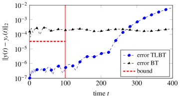
All following computations are carried out in MATLAB^®  8.0.0.783 on a Intel^®Xeon^®CPU X5650 (2.67GHz, 48 GB RAM). We use the rail model from the Oberwolfach benchmark collection which represents a finite element discretization of a cooling process of a steel rail. It provides symmetric positive and negative definite matrices $M$ and, respectively, $A$, as well as $B\in\mathbb{R}^{n\times 7}$, $C\in\mathbb{R}^{6\times n}$. We begin with the coarsest discretization level with $n=1357$ which still allows to compute the matrix exponentials and Lyapunov solutions by direct methods. The final time is $\bar{T}=100$, the input chosen as $u(t)=50\mathbf{1}_{7}$ ($\mathbf{1}_{h}:=[1,\ldots,1]^{T}\in\mathbb{R}^{h}$), and the time integration is carried out using an implicit midpoint rule until $T=400$ with a fixed time step $\delta t=0.04$. We generate reduced order models of dimension $r=40$ by both BT and TLBT. Figure 1 shows the obtained errors $\|y(t)-y_{r}(t)\|_{2}$ and the bound (11), clearly indicating that the proposed bound is valid. Of course, after leaving $[0,\bar{T}]$, (11) is no longer valid and $\|y(t)-y_{r}(t)\|_{2}>\epsilon\left\|u\right\|_{L^{2}_{\bar{T}}}$ for some $t>\bar{T}$. We also see that ordinary BT provides less accurate reduced order models. It is important to point out that almost identical results were obtained if low-rank Gramian approximations computed by rational Krylov subspace methods [6, 13] are used. In particular, running the method for the restricted Gramians with the same settings as in [13] led to $|\epsilon^{\text{approx.}}-\epsilon^{\text{exact}}|\approx 1.6\cdot 10^{-9}$ and visually indistinguishable error norms $\|y(t)-y_{r}(t)\|_{2}$.

Figure 1: Results obtained by BT and TLBT for small rail model ($n=1357$, $\bar{T}=100$, $u(t)=50\mathbf{1}_{7}$, $r=40$).

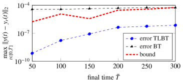
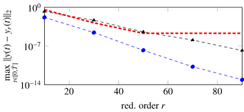
We continue by investigating the influence of the final time $\bar{T}$ and the reduced order $r$ to $\max\limits_{t\in[0,{\bar{T}}]}\|y(t)-y_{r}(t)\|_{2}$ and (11). The results are visualized in Figure 2. For the top plot we fixed $\bar{T}=100$ and varied the reduced order $r=10,\ldots,100$. Apparently, TLBT achieves smaller errors than BT for increasing $r$. After some value of $r$, the bound (11) appears to stagnate and fails to capture the decreasing behavior of the error. The bottom plot shows the results for a fixed $r=50$ but different final times $\bar{T}=50,\ldots,300$ which for TLBT requires, naturally, computing (approximations of) the matrix exponentials and $P_{\bar{T}},\leavevmode\nobreak\ Q_{\bar{T}}$ for each value of $\bar{T}$. The results indicate that increasing $\bar{T}$ also increases the achieved error and the bound (11) appears to capture this behavior. As investigated for TLBT in [13], for even larger final times $\bar{T}$, TLBT will at some point produce errors which are very close to those of BT.

Figure 2: Influence of $r$ (top) and $\bar{T}$ (bottom) for small rail model.

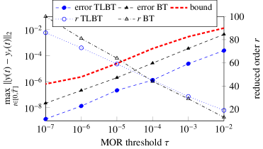
Next we experiment with a larger version of the rail model with $n=79841$. This size requires using low-rank solution factors of the Gramians. We set $u(t)=u_{*}(t):=[\sin(4t\pi/100),\cos(t\pi/100),3,\operatorname{e}^{-2t},\cos(t/100)\operatorname{e}^{-t},\tfrac{1}{1+t^{2}},\tfrac{1}{1+\sqrt{t}}]^{T}$ and $\bar{T}=150$. Motivated by Theorem 2.3, we experiment with an automatic determination of the reduced order $r$ s.t. $\sum_{i=r+1}^{\hat{n}}\sigma_{i,\bar{T}}\leq\tau$ for some specified tolerance $0<\tau\ll 1$ and $\hat{n}:=\min(\text{rank}(Z_{P_{\bar{T}}}),\text{rank}(Z_{Q_{\bar{T}}}))$, i.e., similar as in unrestricted BT. The obtained reduced orders $r$ in BT and TLBT, as well as the largest errors in $[0,\bar{T}]$ and (11) are shown in Figure 3 against different values $\tau=10^{-7},\ldots,10^{-2}$.

TLBT again achieves smaller errors than BT and approximately two orders of magnitude smaller than $\tau$. Note that the obtained reduced orders $r$ of TLBT are for $\tau=10^{-4},10^{-3},10^{-2}$ slightly larger than those of BT. This experiment nevertheless suggests that choosing the order $r$ in TLBT automatically by looking at the time-limited singular values is as reliable as in BT.

Figure 3: Automatically adjusted orders $r$, maximum errors, bound  (11) against tolerances $\tau$ for the larger rail model ($n=79841$, $\bar{T}=150$, $u(t)=u_{*}(t)$).

5 Conclusion

In this paper, we have studied time-limited balanced truncation, an alternative to conventional balanced truncation. This scheme can outperform the conventional ansatz when seeking for a good reduced order model on a certain finite time interval but, so far, no theory on error bounds has been established. Therefore, we proved an $\mathcal{H}_{2}$ error bound in this work. We provided two different representations for the bound. One is appropriate for practical computations, whereas the other one shows that the time-limited singular values can be used as well in order to determine a suitable reduced order dimension. This paper also contains numerical experiments in which we presented the performance of the error bound.

References

• [1] A. C. Antoulas. Approximation of large-scale dynamical systems. Advances in Design and Control 6. Philadelphia, PA: Society for Industrial and Applied Mathematics (SIAM), 2005.
• [2] P. Benner, T. Damm, and Y. R. R. Cruz. Dual pairs of generalized Lyapunov inequalities and balanced truncation of stochastic linear systems. IEEE Trans. Autom. Contr., 62(2):782–791, 2017.
• [3] P. Benner and M. Redmann. Model Reduction for Stochastic Systems. Stoch PDE: Anal Comp, 3(3):291–338, 2015.
• [4] P. Benner and J. Saak. Numerical solution of large and sparse continuous time algebraic matrix Riccati and Lyapunov equations: a state of the art survey. GAMM Mitteilungen, 36(1):32–52, August 2013.
• [5] T. Damm and P. Benner. Balanced truncation for stochastic linear systems with guaranteed error bound. Proceedings of MTNS–2014, Groningen, The Netherlands, pages 1492–1497, 2014.
• [6] V. Druskin and V. Simoncini. Adaptive rational Krylov subspaces for large-scale dynamical systems. Systems and Control Letters, 60(8):546–560, 2011.
• [7] M. Freitag and M. Redmann. Balanced truncation and singular perturbation approximation model order reduction for stochastically controlled linear systems. Technical report, WIAS Preprint No. 2339, 2016.
• [8] W. Gawronski and J. Juang. Model reduction in limited time and frequency intervals. Int. J. Syst. Sci., 21(2):349–376, 1990.
• [9] K. Glover. All optimal Hankel-norm approximations of linear multivariable systems and their L-error norms. Internat. J. Control, 39(6):1115–1193, 1984.
• [10] G. H. Golub and C. F. Van Loan. Matrix Computations. Johns Hopkins University Press, Baltimore, fourth edition, 2013.
• [11] L. Grasedyck. Existence of a low rank or H𝐻H-matrix approximant to the solution of a Sylvester equation. Numer. Lin. Alg. Appl., 11:371–389, 2004.
• [12] N.J. Higham. Functions of Matrices: Theory and Computation. Society for Industrial and Applied Mathematics, Philadelphia, PA, USA, 2008.
• [13] P. Kürschner. Balanced truncation model order reduction in limited time intervals for large systems. arXiv e-print 1707.02839, Cornell University, 2017. Math.NA.
• [14] B. C. Moore. Principal component analysis in linear systems: Controllability, observability, and model reduction. IEEE Trans. Autom. Control, 26:17–32, 1981.
• [15] M. Redmann and P. Benner. An H2subscript𝐻2H_{2}-Type Error Bound for Balancing-Related Model Order Reduction of Linear Systems with Lévy Noise. Systems and Control Letters, 105:1–5, 2017.
• [16] V. Simoncini. Computational methods for linear matrix equations. SIAM Rev., 38(3):377–441, 2016.