A regularity structure for rough volatility
Abstract.
A new paradigm recently emerged in financial modelling: rough (stochastic) volatility, first observed by Gatheral et al. in high-frequency data, subsequently derived within market microstructure models, also turned out to
capture parsimoniously key stylized facts of the entire implied volatility surface, including extreme skews that were thought to be outside the scope of stochastic volatility. On the mathematical side, Markovianity and, partially,
semi-martingality are lost. In this paper we show that Hairer’s regularity structures, a major extension of rough path theory, which caused a revolution in the field of stochastic partial differential equations, also provides a new and powerful tool to analyze rough volatility models.
Dedicated to Professor Jim Gatheral on the occasion of his 60th birthday.
1. Introduction
We are interested in stochastic volatility (SV) models given in Itô differential form
| (1.1) |
Here, is a standard Brownian motion and (resp. ) are known as stochastic volatility (resp. variance) process. Many classical Markovian asset price models fall in this framework, including Dupire’s local volatility model, the SABR -, Stein-Stein - and Heston model. In all named SV model, one has Markovian dynamics for the variance process, of the form
| (1.2) |
constant correlation is incorporated by working with a 2D standard Brownian motion ,
This paper is concerned with an important class of non-Markovian (fractional) SV models, dubbed rough volatility (RV) models, in which case (equivalently: ) is modelled via a fractional Brownian motion (fBM) in the regime .111Volatility is not a traded asset, hence its non-semimartingality (when ) does not imply arbitrage. The terminology ”rough” stems from the fact that in such models stochastic volatility (variance) sample paths are -Hölder, hence “rougher” than Brownian paths. Note the stark contrast to the idea of ”trending” fractional volatility, which amounts to take . The evidence for the rough regime (recent calibration suggest as low as ) is now overwhelming - both under the physical and the pricing measure, see e.g. [1, 24, 25, 27, 4, 19, 42]. Much attention in theses reference has in fact been given to ”simple” rough volatility models, by which we mean models of the form
| (1.3) | |||||
| (1.4) | |||||
| (1.5) | with |
In other words, volatility is a function of a fractional Brownian motion, with (fixed) Hurst parameter.222Following [4] we work with the Volterra- or Riemann-Liouville fBM, but other choices such as the Mandelbrot van Ness fBM, with suitably modified kernel , are possible. Note that, in contrast even to classical SV models, the stochastic volatility is explicitly given, and no rough / stochastic differential equation needs to be solved (hence ”simple”). Rough volatility not only provides remarkable fits to both time series and option pricing problems, it also has a market microstructure justification: starting with a Hawkes process model, Rosenbaum and coworkers [16, 17, 18] find in the scaling limit such that
| (1.6) | |||||
| (1.7) |
with stochastic Volterra dynamics that provide a natural generalization of simple rough volatility.
1.1. Markovian stochastic volatility models
For comparison with rough volatility, Section 1.2 below, we first mention a selection of tools and methods well-known for Markovian SV models.
-
•
PDE methods are ubiquitous in (low-dimensional) pricing problems, as are
-
•
Monte Carlo methods, noting that knowledge of strong (resp. weak) rate (resp. ) is the grist in the mills of modern multilevel methods (MLMC);
-
•
Quasi Monte Carlo (QMC) methods are widely used; related in spirit we have the Kusuoka–Lyons–Victoir cubature approach, popularized in the form of Ninomiya–Victoir (NV) splitting scheme, nowadays available in standard software packages;
-
•
Freidlin–Wentzell theory of small noise large deviations is essentially immediately applicable, as are various “strong“ large deviations (a.k.a. exact asymptotics) results, used e.g. the derive the famous SABR formula.
For several reasons it can be useful to write model dynamics in Stratonovich form: From a PDE perspective, the operators then take sum-square form which can be exploited in many ways (Hörmander theory, naturally linked to Malliavin calculus …). From a numerical perspective, we note that the cubature / NV scheme [43] also requires the full dynamics to be rewritten in Stratonovich form. In fact, viewing NV as level- cubature, in sense of [40], its level- simplification is nothing but the familiar Wong-Zakai approximation result for difffusions. Another financial example that requires a Stratonovich formulation comes from interest rate model validation [13], based on the Stroock–Varadhan support theorem. We further note, that QMC (e.g. Sobol’) works particularly well if the noise has a multiscale decomposition, as obtained by interpreting a (piece-wise) linear Wong-Zakai approximation, as Haar wavelet expansion of the driving white noise.
1.2. Complications with rough volatility
Due to loss of Markovianity, PDE methods are not applicable, and neither are (off-the-shelf) Freidlin–Wentzell large deviation estimates (but see [19]). Moreover, rough volatility is not a semi-martingale, which complicates, to say the least, the use of several established stochastic analysis tools. In particular, rough volatility admits no Stratonovich form. Closely related, one lacks a (Wong-Zakai type) approximation theory for rough volatility. To see this, focus on the “simple” situation, that is (1.1), (1.3) so that
| (1.8) |
Inside the (classical) stochastic exponential we have the martingale term
| (1.9) |
and, in essence, the trouble is due to underbraced, innocent looking Itô-integral. Indeed, any naive attempt to put it in Stratonovich form,
| (1.10) |
or, in the spirit of Wong-Zakai approximations,
| (1.11) |
must fail whenever . The Itô-Stratonovich correction is given by the quadratic covariation, defined (whenever possible) as the limit, in probability, of
| (1.12) |
along any sequence of partitions with mesh-size tending to zero. But, disregarding trivial situations, this limit does not exist. For instance, when fractional scaling immediately gives divergence (at rate ) of the above bracket approximation. This issues also arises in the context of option pricing which in fact is readily reduced (Theorem 1.3 and Section 6) to the sampling of stochastic integrals of the afore-mentioned type, i.e. with integrands on a fractional scale. All theses problems remain present, of course, for the more complicated situation of “non-simple” rough volatility (Section 5) .
1.3. Description of main results
With motivation from singular SPDE theory, such as Hairer’s work on KPZ [32] and the Hairer-Pardoux “renormalized” Wong-Zakai theorem [35], we provide the closest there is to a satisfactory approximation theory for rough volatility. This starts with the remark that rough path theory, despite its very purpose to deal with low regularity paths, is not applicable
To state our basic approximation results, write for a suitable (details below) approximation at scale to white noise, with induced approximation to fBM, denoted by . Throughout, the Hurst parameter is fixed and is a smooth function, such that (1.8) is a (local) martingale, as required by modern financial theory.
Theorem 1.1.
Consider simple rough volatility with dynamics , i.e. driven by Brownians and with constant correlation . There exist -peridioc functions , with diverging averages such that a Wong-Zakai result holds of the form in probability and uniformly on compacts, where
Similar results hold for more general (“non-simple”) RV models.
Remark 1.2.
When , this result is an easy consequence of Itô-Stratonovich conversion formulae. In the case of interest, Theorem 1.1 provides the interesting insight that genuine renormalization, in the sense of subtracting diverging quantities is required if and only if correlation is non-zero. This is the case in equity (and many other) markets [4]. Also note that naive approximations , without subtracting the -term, will in general diverge.
In order to formulate implications for option pricing, define the Black-Scholes pricing function
| (1.13) |
where denotes a standard normal random variable. We then have
Theorem 1.3.
With as in Theorem 1.1, define the renormalized integral approximation,
| (1.14) |
and also approximate total variance,
Then the price of a European call option, under the pricing model (1.1), (1.3), struck at with time to maturity, is given as
where
| (1.15) |
Similar results hold for more general (“non-simple”) RV models.
From a mathematical perspective, the key issue in proving the above theorems is to establish convergence of the renormalized approximate integrals
| (1.16) |
It is here that we find much inspiration from singular SPDE theory, which also requires renormalized approximations for convergence to the correct Itô-object. Specifically, we see that the theory of regularity structures [31], which essentially emerged from rough paths and Hairer’s KPZ analysis (see [23] for a discussion and references), is a very appropriate tool for us. This adds to the existing instances of regularity structures (polynomials, rough paths, many singular SPDEs …) an interesting new class of examples which on the one hand avoids all considerations related to spatial structure (notably multi-level Schauder estimates; cf. [31, Ch.5]), yet comes with the genuine need for renormalization. In fact, since we do not restrict to mollifier approximations (this would rule out wavelet approximation of white noise!) our analysis naturally leads us to renormalization functions. In case of mollifier approximations, i.e. is the -mollifciation obtained by convolution of with a rescaled mollifier function, say ), which is the usual choice of Hairer and coworkers [32, 31, 11], the renormalization function turns out to constant (since is still stationary); in this case
with explicitly given as integral, cf. (3.13). If, on the other hand, we consider a Haar wavelet approximation of white noise, very natural from a numerical point of view, 333Other wavelet choices are possible. In particular, in case of fractional noise, Alpert-Rokhlin (AR) wavelets have been suggested for improved numerical behaviour; cf. [28] where this is attributed to a series of works of A. Majda and coworkers. A theoretical and numerical study of AR wavelets in the rough vol context is left to future work.
| (1.17) |
It is natural to ask if can be replaced, after all, by its (since : diverging) mean . For the answer yes, with an interesting phase transition when , cf. Section 3.2.
From a numerical simulation perspective, Thereom 1.3 is a step forward as it avoids any sampling related to the other factor . A brute-force approach then consists in simulating a scalar Brownian motion , followed by computing by Itô/Riemann Stieltjes approximations of . However, given the singularity of Volterra-kernel , this is not advisable and it is preferable to simulate the two-dimensional Gaussian process with covariance readily available. A remaining problem is that the rate of convergence
with taken in a partition of mesh-size , is very slow since has little regularity when is small. (Gatheral and co-authors [27, 4] report ) . It is here that higher-order approximations come to help and we have included quantitative estimates, more precisely: strong rates, throughout. An analysis of weak rates will be conducted elsewhere, as is the investigation of multi-level algorithms (cf. [6] for MLMC for general Gaussian rough differential equations). Recall that the design of MLMC algorithms requires knowledge of strong rates. Numerical aspects are further explored in Section 6.
The second set of results concerns large deviations for rough volatility. Thanks to the contraction principle and fundamental continuity properties of Hairer’s reconstruction map, the problem is reduced to understanding a LDP for a suitable enhancement of the noise. This approach requires (sufficiently) smooth coefficients, but comes with no growth restrictions which is indeed quite suitable for financial modelling: we improve the Forde-Zhang (simple rough vol) short-time large deviations [19] such as to include of exponential type, a defining feature in the works of Gatheral and coauthors [27, 4]. (Such an extension is also subject of a recent preprint [38] and forthcoming work [30].)
Theorem 1.4.
Remark 1.5.
A potential short-coming is the non-explicit form of the rate function, in the sense that even geometric or Hamiltonian descriptions of the rate function (classical in Markovian setting, see e.g [3, 8, 14, 15, 7]), which led to the famous SABR volatility smile formula, is lost. A partial remedy here is to move from large deviations to (higher order) moderate deviations, which restores analytic tractability and still captures the main feature of the volatiliy smile close to the money. This method was introduced in a Markovain setting in [20], the extension to simple rough volatility was given in [5], relying either on [19] or the above Theorem 1.4.
We next turn to non-simple rough volatility, motivated by Rosenbaum and coworkers [16, 17, 18], and consider the stochastic Itô–Volterra equation
with corresponding rough SV log-price process given by
(For simplicity, we here consider to be bounded, with bounded derivatives of all orders.) For , let be the unique solution to the integral equation
and define and . Then we have the following extension of Theorem 1.4 (and also [19, 38, 30]) to non-simple rough volatility:
Theorem 1.6.
Let be the log-price under non-simple rough SV. Then satisfies a LDP with speed and rate function given by
| (1.19) |
Remark 1.7.
We showed in [5, Cor.11] (but see related results by Alos et al. [2] and Fukasawa [24, 25]) that in the previously considered simple rough volatility models, now writing instead of , the implied volatility skew behaves, in the short time limit, as where in our setting computes to . (The blowup as is a desired feature, in agreement with steep skews seen in the market.) To first order , from which one obtains a skew-formula in the non-simple rough volatility case of the form,
Following the approach of [5], Theorem 1.6 not only allows for rigorous justification but also for the computation of higher order smile features, though this is not pursued in this article. In the case of classical (Markovian) stochastic volaility, , and specializing further to , so that (resp. ) models stochastic (resp. spot) volatility, this reduces precisely to the popular skew formula Gatheral’s book [26, (7.6)], attributed therein to Medvedev–Scaillet. In the case of rough Heston, where models stochastic variance, cf. (5.1), we have and this leads to the following (rough Heston, implied volatility) short-dated skew formula
(multiply with to get the implied variance skew, again in agreement with Gatheral [26, p.35]); this may be independently verified via the characteristic function obtained in [17].
Structure of the article. In Section 2 we reduce the proofs of Theorems 1.1 and 1.3 to the key convergence issue, subject of Section 3. In Section 4 we consider the structure for two-dimensional noise, necessary to study the asset price process. Section 5 then discusses the case of non-trivial dynamics for rough volatility. Some numerical results are presented in , followed by several appendices with technical details. From Section 3 all our work relies on the framework of Hairer’s regularity structures. There seems to be no point in repeating all the necessary definitions and terminology, which the reader can find in [32, 31, 33, 23] and a variety of survey papers on the subject. Instead, we find it more instructive to substantiate our KPZ inspiration and in the next section introduce, informally, all relevant objects from regularity structures in this context.
1.4. Lessons from KPZ and singular SPDE theory
The absence of a good approximation theory is a defining feature of all singular SPDE recently considered by Hairer, Gubinelli et al. (and now many others). In particular, approximation of the noise (say, -mollification for the sake of argument) typically does not give rise to convergent approximations. To be specific, it is instructive to recall the universal model for fluctuations of interface growth given by the Kardar–Parisi–Zhang (KPZ) equation
with space-time white noise . As a matter of fact, and without going in further detail, there is a well-defined (“Cole-Hopf”) Itô-solution , but if one considers the equation with -mollified noise, then diverges with . In this sense, there is a fundamental lack of approximation theory and no Stratonovich solution to KPZ exists. To see the problem, take for simplicity and write
with space-time convolution and heat-kernel
One can proceed with Picard iteration
but there is an immediate problem with , (naively) defined -to-zero limit of , which does not exist. However, there exists a diverging sequence such that, in probability,
The idea of Hairer, following the philosophy of rough paths, was then to accept
as enhancement of the noise (”model”) upon which solution depends in pathwise robust fashion. This unlocks the seemingly fixed (and here even non-sensical) relation
Loosely speaking, one has
Theorem 1.8 (Hairer).
There exist diverging constants such that a Wong-Zakai444Hairer–Pardoux [35] derive the KPZ result as special case of a Wong-Zakai result for Itô-SPDEs. result holds of the form , in probability and uniformly on compacts, where
Similar results hold for a number of other singular semilinear SPDEs.
In a sense, this can be traced back to the Milstein-scheme for SDEs and then rough paths: Consider , with for simplicity, and consider the 2nd order (Milstein) approximation
One has to unlock the seemingly fixed relation
for there is a choice to be made. For instance, the last term can be understood as Itô-integral or as Stratonovich integral (and in fact, there are many other choices, see e.g. the discussion in [23].) It suffices to take this thought one step further to arrive at rough path theory: accept as new (analytic) object, which leads to the main (rough path) insight
In comparison,
| SPDE theory à la Hairer | ||||
| = | analysis based on (renormalized) enhanced noise . |
Inside Hairer’s theory: 555In the section only, following [23], symbols will be coloured. As motivation, consider the Taylor-expansion (at ) of a real-valued smooth function,
can be written as abstract polynomial (“jet”) at ,
with, necessarily, . If we “realize” these abstract symbols again as honest monomials, i.e. and extend linearly, then we recover the full Taylor expansion:
Hairer looks for solution of this form: at every space-time point a jet is attached, which in case of KPZ turns out - after solving an abstract fixed point problem - to be of the form
As before, every symbol is given concrete meaning by “realizing” it as honest function (or Schwartz distribution). In particular,
| (1.20) |
and then, more interestingly,
| (1.21) |
This realization map is called “model” and captures exactly a typical, but otherwise fixed, realization of the noise (mollified or not) together with some enhancement thereof, renormalized or not. For instance, writing for the realization map for renormalized enhanced noise, one has
where indicates suitable centering at . Mind that takes values in a (finite) linear space spanned by (sufficiently many) symbols,
The map is an example of a modelled distribution, the precise definition is a mix of suitable analytic and algebraic conditions (similar to the notation of a controlled rough path).
The analysis requires keeping track of the degree (a.k.a. homogeneity) of each symbol. For instance, (related to the Hölder regularity of the realized object one has in mind), etc. All these degrees are collected in an index set. Last not least, in order to compare jets at different points (think ), use a group of linear maps on , called structure group. Last not least, the reconstruction map uniquely maps modelled distributions to function / Schwartz distributions. (This can be seen as generalization of the sewing lemma, the essence of rough integration, see e.g. [23], which turns a collection of sufficiently compatible local expansions into one function / Schwartz distribution.) In the KPZ context, the (Cole-Hopf Itô) solution is then indeed obtained as reconstruction of the abstract (modelled distribution) solution .
Acknowledgment: The authors acknowledge financial support from DFGs research grants BA5484/1 (CB, BS) and FR2943/2 (PKF, BS), the ERC via Grant CoG-683166 (PKF), the ANR via Grant ANR-16-CE40-0020-01 (PG) and DFG Research Training Group RTG 1845 (JM).
Participants of Global Derivatives 2017 (Barcelona) and Gatheral 60th Birthday conference (CIMS, NYU) are thanked for the feedback.
2. Reduction of Theorems 1.1 and 1.3
In the context of these theorems, we have
| (2.1) |
where we recall that
All approximations, and converge uniformly to the obvious limits, so that it suffices to understand the convergence of the stochastic integral. Note that is heavily correlated with but independent of . The difficult interesting part is then indeed (1.16), i.e.
| (2.2) |
which is the purpose of Theorem 3.24. For the other part, due to independence no correction terms arise and we have (with details left to the reader) with convergence in probability and uniformly on compacts in . The convergence result of Theorems 1.1 then follows readily.
As for pricing, Theorem 1.3, consider the call payoff . An elementary conditioning argument (first used by Romano–Touzi in the context of Markovian SV models) w.r.t. , then shows that the call price is given as expection of
Specializing to the case , in combination with Theorem 3.24, then yields Theorem 1.3 . Remark that extensions to non-simple RV are immediate from suitable extensions of Theorem 3.24, as discussed in 5.2.
3. The rough pricing regularity structure
In this section we develop the approximation theory for integrals of the type . In the first part we present the regularity structure and the associated models we will use. In the second part we apply the reconstruction theorem from regularity structures to conclude our main result, Theorem 3.24.
3.1. Basic pricing setup
We are given a Hurst parameter , associated to a fractional Brownian motion (in the Riemann-Liouville sense) , and fix an arbitrary and an integer
so that
| (3.1) |
At this stage, we can introduce the “level-” model space
| (3.2) |
where denotes the vector space generated by the (purely abstract) symbols in . We will sometimes write
so that .
Remark 3.1.
The interpretation for the symbols in is as follows: should be understood as an abstract representation of the white noise belonging to the Brownian motion , i.e. where the derivative is taken in the distributional sense. Note that since we set for we have for . The symbol has the intuitive meaning “integration against the Volterra kernel”, so that represents the integration of white noise against the Volterra kernel
which is nothing but the fractional Brownian motion . Symbols like or should be read as products between the objects above. These interpretations of the symbols generating will be made rigorous by the model in the next subsection. Every symbol in is assigned a homogeneity, which we define by
We collect the homogeneities of elements of in a set , whose minimum is . Note that the homogeneities are multiplicative in the sense that, for .
At last, our regularity comes with a structure group , an (abstract) group of linear operators on the model space which should satisfy and for and . We will choose given by
and for for which is defined.
The limiting model
Let be a Brownian motion on and extend it to all of by requiring for . We will frequently use the notations
| (3.3) |
which denote the Itô integral and the Skohorod integral (which boils down to an Itô integral whenever the integrand is adapted). From we construct now the fractional Riemann-Liouville Brownian motion with Hurst index as
where denotes the Volterra kernel. We also write .
To give a meaning to the product terms we follow the ideas from rough paths and define an “iterated integral” for as
| (3.4) |
satisfies a modification of Chen’s relation
Lemma 3.2.
Proof.
Direct consequence of the binomial theorem.
We extend the domain of to all of by imposing Chen’s relation for all , i.e. we set for
| (3.6) |
We are now in the position to define a model that gives a rigorous meaning to the interpretation we gave above for . Recall that in the theory of regularity structures a model is a collection of linear maps , for indices that satisfiy
| (3.7) | |||
| (3.8) | |||
| (3.9) |
where the bounds hold uniformly for , any in a compact set and for with and with compact support in the ball .
We will work with the following “Itô” model , and (occasionally) write to avoid confusion with a generic model, also denoted by , which renders more precisely our interpretations of the elements of .
We extend both maps from to by imposing linearity.
Lemma 3.3.
The pair as defined above defines (a.s.) a model on .
Proof.
The only symbol in on which (3.7) is not straightforward is , where the statement follows by Chen’s relation. The bounds (3.8) and (3.9) follow for trivially and for by the Hölder regularity of . It is further straightforward to check the condition (3.9) by using the rule so that we are only left with the task to bound . Following along the lines of proof [23, Theorem 3.1] it follows (where denotes a random constant with ), so that
As we will see below in subsection 3.2 this model is the toolbox from which we can build pathwise Itô integrals of the type . For an approximation theory for such expressions we are in need of a comparable setup that describes approximations, which will be achieved by introducing a model .
The approximating model
The whole definition of the model is based on the object . It is therefore natural to build an approximating model by replacing by some modification that converges (as a distribution) to as .
The definition of will be based on an object which should be thought of as an approximation to the Delta dirac distribution. Our purpose to build from wavelets, which can be as irregular as the Haar functions. We find it therefore convenient to allow to take values in the Besov space which covers functions like .
Remark 3.4.
We shortly recall the definition of the Besov space (see for example [41]) although this will here only be explicitely used in the proof of Lemma 3.16 in the appendix. Given a compactly supported wavelet basis , we set
and define to be those functions (or distributions if ) for which this norm is finite.
Definition 3.5.
In the following we call a measurable, bounded function with the following properties
-
•
for all .,
-
•
the map is bounded and measurable for some .
-
•
,
-
•
,
-
•
for any and some .
Example 3.6.
There are two examples which are of particular interest for our purposes
-
•
We say that “comes from a mollifier”, by which we mean that there is symmetric, compactly supported -function , which integrates to such that
-
•
A further interesting example is the case where “comes from a wavelet basis”. Consider only and choose compactly supported -valued father wavelets (e.g. the Haar father wavelets ) and set
Note that we could also add some generations of mother wavelets in this choice.
Note that (locally) is contained in (recall: ), so that due to we can set
which is a Gaussian process and pathwise measurable and locally bounded. For (maybe stochastic) integrands we introduce the notations
and if takes values in some (non-homogeneous) Wiener chaos induced by we also introduce
| (3.10) |
where denotes the Wick product. Note that these two objects do in general not coincide. The motive for using the same symbol “” as in (3.3) is that (3.10) can be seen as the Skohorod integral with respect to the Gaussian stochastic measure induced by the Gaussian process (for the notion of Wick products and Skohorod integrals and their links see e.g. [39]).
We now define an approximate fractional Brownian motion by setting
which has the expected regularity as it is shown in the following lemma.
Lemma 3.7.
On every compact time intervall we have the estimates
uniformly in for any and and where are random constants that are (uniformly) bounded in for .
Proof.
The proof is elementary but a bit bulky and therefore postponed to the appendix.
Finally we can give the definition of the approximative model , the “canonical” model built from the approximate (and hence regular) noise .
Lemma 3.8.
The pair as defined above is a model on .
Proof.
The definition of this model is justified by the fact that application of the reconstruction operator (as in Lemma 3.22) yields integrals
| (3.11) |
As we pointed out already in section 1, there is no hope that integrals of this type will converge as if . This can be cured by working with a renormalized model instead.
The renormalized model
From the perspective of regularity structures the fundamental reason why integrals like (3.11) fail to converge to
lies in the fact that the corresponding models will not satisfy in a suitable norm. To see what is going on we will first rewrite
Lemma 3.9.
For we have
where denotes the Skorokhod integral and denotes the Volterra kernel. Note that in the second term the domain of integration is actually .
Remark 3.10.
Our notation reflects a close relation between the Skorokhod integral and the Wick product. Indeed, when , with summation over a finite partition of , and each a (non-adapted) random variable in a finite Wiener-Itô chaos, it follows from [39, Thm 7.40] that . Passage to -limits is then standard. See also [44] and the references therein.
Proof.
We prove this by reexpressing . For we have already
so that it remains to see what happens for . With relation (3.6) we have in this case
where we use for the sake of concision formal notation, which is easy to translate to a rigorous formulation. Using the fact that for Gaussians we have
| (3.12) |
(a consequence of [39, Theorems 3.15, 7.33]), we obtain
Using and for we can reformulate this and obtain
(An alternative derivation of the above Skorokohod form can be given in terms of [45, Thm 3.2].) Since the claim follows.
Let us also reexpress the approximating model in suitable form.
Lemma 3.11.
Proof.
Comparing the expressions in Lemma 3.11 and 3.9 we see that we morally have to subtract
from the model, which will give us a new model . Of course we have to be careful that this step preserves “Chen’s relation” , see Theorem 3.13 below.
If we interpret as an approximation to the Volterra-kernel we see that the expression
will correspond to something like “” in the limit . We have indeed the following upper bound.
Lemma 3.12.
For all we have
Proof.
Our hope is now that the new model converges to in a suitable sense. Similar to [31, (2.17)] we define the distance between two models and on a compact time interval as
| (3.19) |
where denotes the absolute value of the coefficient of the symbol with and where the first supremum runs over with . We will also need
We are now ready to give the fundamental result of this subsection which plays a key role in our approximation theory. Recall that the (minimal) homogeneity which corresponds to being Hölder with exponent .
Theorem 3.13.
Define, for every , the linear map given by, for
and on all remaining symbols in . Then
defines a (“renormalized”) model on and on compact time intervals we have
| (3.20) |
for any and . In particular, we have “almost rate ” for large enough.
Remark 3.14.
In the special case of the level-2 Brownian rough path (i.e. ) the above result is in precise agreement with known results (even though the situation here is simpler since we are dealing with scalar Brownian). More specifically, we don’t see the usual (strong) rate “almost” but have to subtract the Hölder exponent used in the rough path / model topology (here: ) which exactly leads to the rate “almost ”. Since entails the condition , we see that , exactly as given e.g. in in [23, Ex. 10.14]. A better rate can be achieved by working with higher-level rough path (here: ) and indeed the special case of , but general , can be seen as a consequence of [21]: at the price of working with levels, one can choose arbitrarily close to and so recover the usual “almost” rate. Of course, the case is out of reach of rough path considerations.
Proof.
Since due to Lemma 3.12 we have, for fixed , that and the bound (3.8) is still satisfied. The modification does not lead to a violation of “Chen’s relation”. Indeed, using validity of (3.7) for the original model, we have
We so see that (3.7) is also satisfied after our modification, and then easily conclude that is still a model on . At last, the bound (3.20) is a bit technical and left to Appendix A.
3.2. Approximation and renormalization theory
We now address to central question of how the integral has to be modified to make it convergent against .
The key idea is to combine the convergence result from Theorem 3.13 with Hairer’s reconstruction theorem, which we state below.
We first recall the notion of a modelled distribution, compare [31, Definition 3.1]. We say that a map is in the space for some time horizon if
| (3.21) |
where as above denotes the absolute value of the coefficient of the vector with . Given two models and and two it is also usefull to have the notion of a distance
The reconstruction theorem now states that for a map can be uniquely identified with a distribution that behaves locally like .
Theorem 3.15.
[31, Theorem 3.10]
Given a model , and a there is a unique continuous operator666 denotes the space of distributions that are locally in the Besov space (cmp. [31, Remark 3.8]). such that for any and
| (3.22) |
For two different models and we further have
| (3.23) |
for .
As mentioned earlier we want ourselves to work with compactly supported functions which includes objects like the Haar wavelets. The following Lemma allows us to carry over all bounds.
Lemma 3.16.
Remark 3.17.
This covers in particular functions like .
Proof.
We prove this via wavelet methods in the appendix.
By the notation we mean in the following both and .
To study objects like with the reconstrution theorem we first “expand” the integrand in the regularity structure
On the level of the regularity structure these objects can be multiplied with “noise” which gives a modelled distribution on .
We will analyze by writing it as composition of a (random) modelled distribution with the smooth function . To this end we need
Lemma 3.18.
On the regularity structure introduced in Section 3.1, consider a model which is admissible in the sense
Then
| (3.24) |
defines a modelled distribution. More precisely, .
Remark 3.19.
Proof.
By definition of the modelled distribution space we need to understand the action of on all constituting symbols. Since span a sector, i.e. a space invariant by the action of the structure group, it is clear that
Application of the realization map , followed by evaluation at , immediately identifies as
where we used admissibility and in the last step, a general fact due to the trivial action of the structure group on the symbol with lowest degree. As a consequence , so that, trivially, for any .
For a given (sufficiently smooth) function , and a generic model on our regularity structure, define
Remark that is function-like, i.e. with values in the span of symbols with non-negative degree. From [31, Prop. 3.28] we then have
(In particular, we see that coincides with when is taken as either approximate or renormalized approximate model.) We can also define simply obtained by multiplying it with . The properties of and are summarized in the following lemma.
Lemma 3.20.
Given , there exists such that, for all
We have further for two given models and ,
| (3.25) | ||||
| (3.26) |
where the proportionality constants are, in particular, uniform over all with bounded -norm.
Proof.
Remark 3.21.
In the case when but with no global bounds, the result still holds since we only consider the values of on the range of the continuous function (which is bounded by some ). The resulting bounds then depend linearly on .
In the case of the Itô model (resp. the approximating renormalized models ) we simply denote by (resp. ). We are then allowed to apply Hairer’s reconstruction Theorem 3.15. Note that since we have two models we have two reconstruction operators and . The objects can be written down explicitely.
Lemma 3.22.
We have (a.s.)
Proof.
The proof is in the appendix.
If we take we obtain , so that it is natural to choose as an approximation. However, note that the key property of the reconstruction operator is that it is locally close to the corresponding model so that we have in fact two natural approximations:
We might drop the indices and on and if there is no risk of confusion.
The following theorem, which can be seen as the fundamental theorem of our regularity structure approach to rough pricing shows that these approximations do both converge.
Theorem 3.24.
Fix . For smooth, bounded with bounded derivatives, and as in Definition 3.23 we have
-
(i)
for any and any there exists such that
(3.27) -
(ii)
for every we can pick large enough, such that, for any there exists such that
(3.28)
Remark 3.25.
With regard to (i): although does not depend on any choice of , and nor does its (Itô) limit, the choice of affects the entire regularity structure and so, implicitly also the reconstruction operator used in the definition of , as well as the modelled distribution . The latter, in turn, requires for the construction to make sense. If is chosen arbitrarily close to one, needs to have derivatives of arbitrary order, hence our smoothness assumption.
Remark 3.26.
( of exponential form; [27]) By an easy localization argument one shows that for smooth (but without any further bounds) ones still has
with . The original rough vol model due to [27] makes a point that should be of exponential form. Now, the result with -estimates still holds since we only consider the values of on the range of the continuous function (which is bounded by some ). As pointed out in Remark 3.21, the bounds then depend linearly on . Since, for us, is always a Gaussian model, is a Gaussian process (say, or hence we have (Fernique) Gaussian concentration for . So, for instance if and its derivatives have exponential growth we do have the bounds of the above theorem, for all . This remark justifies in particular the choice and in the numerical discussion of Section 6.
Proof.
Without loss of generality , otherwise split in subintervals. Let us show (3.27).
We then obtain the rate using Theorem 3.13, Lemma 3.20 and (3.19) for the first term and also Theorem 3.15 for the second term. Letting and our total rate can be chosen arbitrary close to .
To obtain the second estimate we can bound with the first inequality in Theorem 3.15.
Non-constant vs. constant renormalization
If comes from a mollifier (cf. Example 3.6) the renormalization that was applied in Theorem 3.13 and thus in Definition 3.23 is a constant, which is the familiar concept one encounters in the study of singular SPDE [32, 31, 11]. If comes from wavelets such as the Haar basis, is usually not constant but a periodic function with period . Thus we see that our analysis gives rise to a “non-constant renormalization”. It is natural to ask if one can do with constant renormalization after all. For the sake of argument, consider , periodic with period , with mean
From Lemma 3.12 it follows that (and its mean) are bounded by , uniformly in . Putting all this together it easily follows that , uniformly over all bounded in , with convergence to zero when . As a consequence, taking , for smooth , we clearly can apply this with any . Hence, by equating the constraints on , we arrive at . The practical consequence then is, with focus on the convergence stated in part (i) of Theorem 3.27 that we can indeed replace non-constant renormalization by a constant, however at the prize of restricting to and with an according loss on the convergence rate. Interestingly, our numerical simulation suggest that no loss occurs and constant renormalization works for any . While we have refrained from investigation this (technical) point further, 777Some computations led us to believe that this question can be settled with the aid of mixed -variation of the covariance function of the Volterra process, cf. [22], which we expected to hold uniformly over approximation. However the amount of work seems in no relation to the main theme of this article. we can understand the mechanism at work by looking at the following toy example: Consider the Ito-integral where is a fBM, but now with Hurst parameter , built, say, as Volterra process over . Using Young integration theory, one can give a pathwise argument that shows that Riemann-Stieltjes approximation converge a.s. (with vanishing rate as ). However, we know from stochastic theory (Itô integration) that this convergence works in (and then in probability) for any . We would thus expect that, when , constant renormalization is still valid, but now the difference only vanishes in mean-square sense (which is what we did in the numerics section).
3.3. The case of the Haar basis
The following special case of the approximations above to is of particular interest for our purposes. We here collect some more concrete formulas that arise in this case.
Let , and and the corresponding coming from this wavelet is then for .
The mollified Volterra-kernel (3.13) then takes the form
A special role is played by diagonal function as a renormalization,
| (3.29) |
We have moreover
where are i.i.d. variables. As approximation we can finally take from Definition 3.23 with partition which gives us
and
As explained at the end of the last section, in these formulas could be replaced by its local mean, the constant
4. The full rough volatility regularity structure
4.1. Basic setup
We want to add an independent Brownian motion, so that we take an additional symbol . We again fix and define a (larger) collection of symbols , with , and then
| (4.1) |
Again we fix and the homogeneity of the other symbols are defined multiplicatively as before.
Also as before, we set with , where and also are independent Brownian motions.
We extend the canonical model to this regularity structure by defining
(the above integral being in Itô sense), and 888Upon setting , the given relation is precisely implied by multiplicativity of .
Arguments similar to the proof of Lemma 3.8 show that this indeed defines a model on .
4.2. Small noise model large deviation
Given we consider the ”small-noise” model on obtained by replacing by , which simply means that
and
Finally, for in , we consider the deterministic model defined by
and
The following lemma and theorem are proved in Appendix B.
Lemma 4.1.
For each , does define a model. In addition, the map is continuous.
Theorem 4.2.
The models satisfy a large deviation principle (LDP) in the space of models with rate and rate function given by
As an immediate corollary we have
Corollary 4.3.
For small, , in the precise sense of a large deviation principle (LDP) for
with speed , and rate function given by
| (4.2) |
where
Remark 4.4.
Proof.
We note that thanks to Brownian resp. fractional Brownian scaling, small noise large deviations translate immediately to short time large deviations, cf. [19].
Although the rate function here is not given in a very useful form, it is possible [5] to expand it in small and so compute (explicitly in terms of the model parameters) higher order moderate deviations which relate to implied volatility skew expansions.
5. Rough Volterra dynamics for volatility
5.1. Motivation from market micro-structure
Rosenbaum and coworkers, [16, 17, 18], show that stylized facts of modern market microstructure naturally give rise to fractional dynamics and leverage effects. Specifically, they construct a sequence of Hawkes processes suitably rescaled in time and space that converges in law to a rough volatility model of rough Heston form
| (5.1) | |||||
(As earlier, independent Brownians.) Similar to the case of the classical Heston model, the square-root provides both pain (with regard to any methods that rely on sufficient smooth coefficients) and comfort (an affine structure, here infinite-dimensional, which allows for closed form computations of moment-generating functions). Arguably, there is no real financial reason for the square-root dynamics999This is also a frequent remark for the classical Heston model. and ongoing work attempts to modify the above square-root dynamics, such as to obtain (something close to) log-normal volatility, put forward as important rough volatility feature by Gatheral et al. [27]. This motivates the study of more general dynamic rough volatility models of the form
| (5.2) | |||||
| (5.3) |
with sufficiently nice functions . (While is still OK in what follows, we assume for a local solution theory and then in fact impose for global existence. (One clearly expects non-explosion under e.g. linear growth, but in order not to stray too far from our main line of investigation we refrain from a discussion.) Remark that plays the role of spot-volatility. Further note that the choice brings us back to the “simple” case with (rough stochastic) volatility considered in earlier sections.
With some good will,101010We are not aware of any literature on mixed Itô-Volterra systems (although expect no difficulties). Here of course, it suffices to first solves for and then construct as stochastic exponential. equation (5.2) fits into the existing theory of stochastic Volterra equations with singular kernels (e.g. [46] or [12]).
5.2. Regularity structure approach
We insist that (5.2) is not a classical Itô-SDE (solutions will not be semimartingales), nor a rough differential equations (in the sense of rough paths, driven by a Gaussian rough path as in [23, Ch.10]). If rough paths have established themselves as a powerful tool to analyze classical Itô-SDE, we here make the point that Hairer’s theroy is an equally powerful tool to analyze stochastic Volterra (resp. mixed Itô-Volterra) equations in the singular regime of interest.
As preliminary step, we have to have to find the correct model space, spanned by symbols which arise by formal Picard iteration. To this end, rewrite (5.2) formally, or as equation for modelled distributions,
| (5.4) |
from which one can guess (or formally derive along [31, Sec. 8.1]) the need for the symbols
We have degrees and then, for subsequent symbols, degree computed as
For a modelled distribution, takes values in the linear span of sufficiently many symbols, the (minimal) number of which is dictated by the Hurst parameter . Loosely speaking, indicates an expansions with -error estimate, in practice easy to see from the degree of the lowest degree symbols that do not figure in the expansion. For example, in case of a “level- expansion” we can expect
since It follows from general theory [31, Thm 4.16] that if , then so is , the composition with a smooth function, and by [31, Thm 4.7] the product with is a modelled distribution in . For both reconstruction and convolution with singular kernels, one needs modelled distributions with positive degree . Given we can then determine which symbols (up to which degree) are required in the expansion. As earlier, fix an integer
(so that ) and see that will do. When , and by choosing small enough, we see that will do. That is, the symbols required to describe are and if one adds the symbols required to describe the right-hand side, one ends up with the level- model space spanned by
which is exactly the model space for the “simple” rough pricing regularity structure, (3.2) in case . When this precise correspondence is no longer true. To wit, in case , taking accordingly, solving (5.3) on the level of modelled distributions will require a (“level-”) model space given by
which is strictly larger than the corresponding level- simple model space given in (3.2). In general, one needs to consider an extended model space , so as to have
(with the understanding that only finitely many such symbols are needed, depending on as explained above). As a result, symbols such as
will appear. At this stage a tree notation (omnipresent in the works of Hairer) would come in handy and we refer to [9] (and the references therein) for a recent attempt to reconcile the tree formalism of branched rough path [29, 34] and the most recent algebraic formalism of regularity structures. (In a nutshell, the simple case (3.2) corresponds to trees where one node has branches; in the present non-simple case symbols branching can happen everywhere.) ) Carrying out the following construction in the general case, , is certainly possible.111111We note that, as the number of symbols tends to infinity. In comparison, as far as we know, among all recently studied singular SPDEs, only the sine-Gordon equation [36] exhibits arbitrarily many symbols. However, the algebraic complexity is essentially the one from branched rough paths and hence the general case requires a Hopf algebraic (Connes-Kreimer, Grossman-Larson …) construction of the structure group (a.k.a. positive renormalization). Although this, and negative renormalization, is well understood ([31, 10], also [9] for a rough path perspective, all complete exposition would lead us to far astray from the main topic of this paper. Hence, for simplicity only, we shall restrict from here on to the level- case (with accordingly) but will mention general results whenever useful.
5.3. Solving for rough volatility
We rewrite (5.3) as equation for modelled distributions in ,
| (5.5) |
(Here are the operators associated to composition with respectively.) We also impose
which is clearly necessary such as to have the product in a modelled distribution space of positive parameter, so that reconstruction, convolution etc. makes sense. Let and pick so that . As explained in the previous section, this exactly allows us to work in the familiar structure of Section 3.1. That is, with ,
with index set and structure group as given in that section. This structure is equipped with the Itô-model, and its (renormalization) approximations. Equation (5.5) critically involves the convolution operator acting on . The general construction [31, Sec. 5] is among the most technical in Hairer’s work, and in fact not directly applicable (our kernel , although -regularizing with ) fails the Assumption 5.4 in [31]) so we shall be rather explicit.
Lemma 5.1.
On the regularity structure of Section 3.1 with , consider a model which is admissible in the sense
Let and set 121212 is extended linearly to all of by taking for symbols ).
Then (i) maps and (ii) , i.e. convolution commutes with reconstruction.
Remark 5.2.
Proof.
(Sketch) The special case was already treated in Lemma 3.18. We only show that, in the general case, necessarily has the stated form but will not check the properties. It is enough to consider with values in and make the ansatz
Applying reconstruction, together with [31, Prop. 3.28] we see that which in turn must equal , provided we postulate validity of (ii). This is the given definition of .
We return to our goal of solving
| (5.6) |
noting perhaps that makes sense for every function-like modelled distribution, say , in which case
| (5.7) |
(Similar remarks apply to , the composition operator associated to ). Recall .
Theorem 5.3.
For any admissible model and , , for any , the equation (5.6) has a unique solution in , and the map is locally Lipschitz in the sense that if and are the solutions corresponding respectively to and ,
with the proportionality constant being bounded when the (resp. and model) norms of the arguments stay bounded.
In addition, if is the canonical Itô model (associated to Brownian resp. fractional Brownian motion, ) then is solves (5.2) in the Itô-sense.
Remark 5.4.
is clearly the (unique) reconstruction of the (unique) solution to the abstract problem. We also checked that is indeed a solution for the Itô-Volterra equation. However, if one desires to know that is the unique strong solution to the stochastic Itô-Volterra equation, it is clear that one has to resort to uniqueness results of the stochastic theory, see e.g. [12].
Proof.
Using the large deviation results obtained in the previous subsection, we can directly obtain a LDP for the log-price
For square-integrable , let be the unique solution to the integral equation
Corollary 5.5.
Let and smooth (without boundedness assumption). Then satisfies a LDP with speed and rate function given by
| (5.8) |
where
Remark 5.6.
Despite our previous limitation to , to approach extends to any and yields the result as stated.
Proof.
Ignoring the second part in which is since is bounded, we let and by scaling we see that
where and , are defined in the same way as , with replaced by and replaced by .
We then note that
where is locally Lipschitz by Theorem 5.3. We can then directly use the fact that satisfy a LDP (Theorem 4.2) with a contraction principle such as Lemma 3.3 in [37] to obtain that satisfies a LDP with rate function
It then suffices to note that is exactly for the solution to (5.6) corresponding to a model and with , and to optimize separately over as in the proof of Corollary 4.3.
We also have an approximation result :
Corollary 5.7.
Let (for simplicity, but see remark below). Then , uniformly on compacts and in probability, where
| (5.9) |
Remark 5.8.
Replacing the renormalization function by its mean is possible, provided . However, unlike the discussion at the end of Section 3.2, this is no more a consequence of quantifying the distributional convergence. In the present context, this is achieved by checking directly model-convergence, which, fortunately, is not much harder. We leave details to the interested reader.
Remark 5.9.
In contrast to the previous statement, the above result is more involved for and additional terms renormalization terms appear, the general description of which would benefit from pre-Lie products, as recently introduced [9].
Proof.
Thanks to Theorem 3.13 and Theorem 5.3 it follows from continuity of reconstruction that
so that the only thing to do is check that solves (5.9). Note that (5.6) implies that one has (omitting upper ’s at all normal and caligraphic …)
and, with (5.7),
But then since is a “smooth” model, in the sense of Remark 3.15. in [31], one has
Since convolution commutes with reconstruction, cf. Lemma 5.1, it follows that is indeed a solution to (5.9).
6. Numerical results
We will now resume where we left off in Section 3.3 and revisit the case of European option pricing under rough volatility. Building on the theoretical underpinnings of Section 3, we present a concise description of the central algorithm of this paper - for simplicity restricted to the unit time interval - and complement the theoretical convergence rates obtained in previous chapters with numerical counterparts. The code used to run the simulations has been made available on https://www.github.com/RoughStochVol.
Concise description. Without loss of generality, set time to maturity . We are interested in pricing a European call option with spot and strike under rough volatility. From Theorem 1.3, we have
| (6.1) |
where the computational challenge obviously lies in the efficient simulation of
As explored in Subsection 3.3, we take a Wong-Zakai-style approach to simulating , that is, we approximate the White noise process on the Haar grid as follows:
Let and choose a Haar grid level such that the stepsize of the Haargrid . Then, for all and , we set
| (6.2) |
which induces an approximation of the fBm
| (6.3) | ||||
| (6.4) |
As outlined before, the central issue is that the object does not converge in an appropriate sense to the object of interest as . This is overcome by renormalizing the object, two possible approaches of which are explored in Subsection 3.3. For the remainder, we will consider the ’simpler’ renormalized object given by
| (6.5) |
where the renormalization object can be one of
| (6.6) |
Coming back to the original question of simulating , we just argued that what we really need to simulate to achieve convergence in a suitable sense is the object , the expressions of which are collected below (note that under an assumed non-constant renormalization the expression (6.5) for has been rewritten to a form more suitable for efficient simulation):
| (6.7) | ||||
| (6.8) |
Numerical convergence rates.
In this subsection, we will discuss strong convergence of the approximative object to the actual object of interest as well as weak convergence of the option price itself as the Haar grid interval size . Specifically, we will be looking at Monte Carlo estimates of our errors, that is, in order to approximate some quantity for some random variable , we will instead be looking at where the are iid samples drawn from the same distribution as . In other words, we need to generate realisations of the bivariate stochastic object , a task that can be vectorized as described below, thus avoiding expensive looping through realisations.
Strong convergence. We verify Theorem 3.24 (i) numerically , albeit in the -sense and - for simplicity - with , i.e. with no explicit time dependence. That is, we are concerned with Monte Carlo approximations of
and we expect an error almost of order .
Remark 6.1.
We choose because this closely resembles the rough Bergomi model (see [4] and below). Also, for the simplest non-trivial choice, , the discretization error is overshadowed by the Monte Carlo error, even for very coarse grids.
Since is a two-dimensional Gaussian process with known covariance structure, it is possible to use the Cholesky algorithm (cf. [4, 5]) to simulate the joint paths on some grid and then use standard Riemann sums to approximate the integral. The value obtained in this way could serve as a reference value for our scheme. However - for strong convergence - we need both objects to be based on the same stochastic sample. For this reason, we find it easier to construct a reference value by the wavelet-based scheme itself, i.e. we simply pick some and consider
| (6.9) |
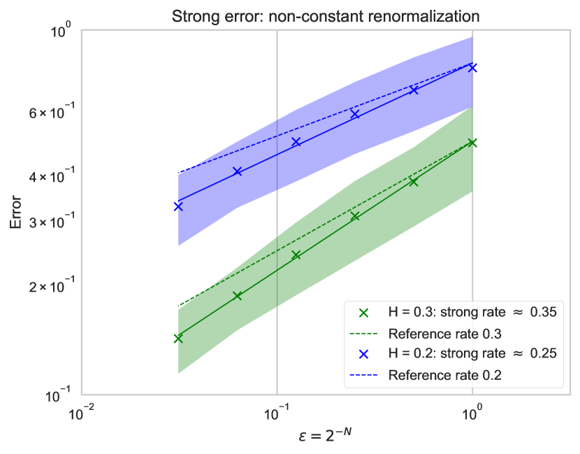
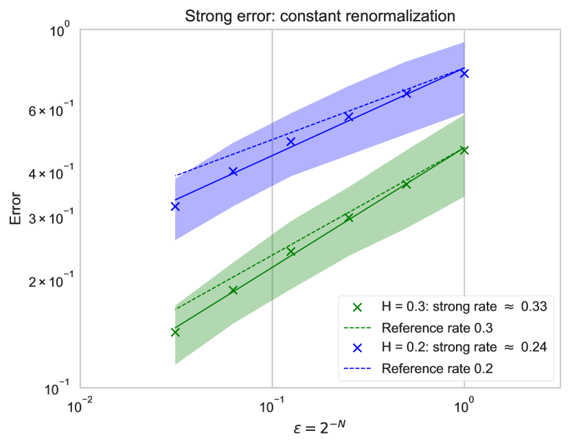
as . As can be seen in Figures 1 and 2, both renormalization approaches stated in (6.6) are consistent with a theoretical strong rate of almost across the full range of (cf. discussion at the end of Section 3.2).
Remark 6.2 (Weak convergence).
In absence of a Markovian structure, a proper weak convergence analysis proves to be subtle, that is, an analysis that - for suitable test functions - yields a rate of convergence for
as , remains an open problem. However, picking , Ito’s isometry yields
| (6.10) |
which we can be approximated numerically. So we can consider
| (6.11) |
as . Our preliminary results indicate that for both renormalization approaches the weak rate seems to be around the strong rate .
Option pricing. We pick a simplified version of the rough Bergomi model [4] where the instantaneous variance is given by
with and denoting spot volatility and volatility of volatility respectively. Let denote the approximation of the call price (6.1) based on , fix some and consider
| (6.12) |
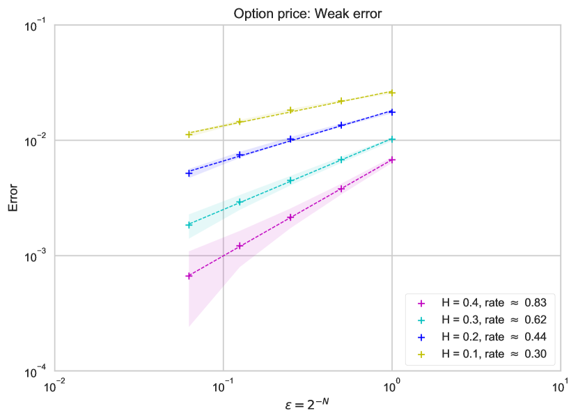
as . Empirical results displayed in Figure 3 indicate a weak rate of across the full range of .
Appendix A Approximation and renormalization (Proofs)
Lemma A.1.
For and we have for
and for
Proof.
This follows from interpolation between and .
Proof of Lemma 3.7 .
Rewriting we have
where we used the Itô isometry in the first and Jensen’s inequality in the second step. Assuming we can split the integral in domains and which yields the bound . Application of equivalence of moments for Gaussian random variables and Kolmogorov’s criterion then shows the first inequality.
The second one follows by interpolation (and once more Kolmogorov) if we can prove that
| (A.1) |
We have, by Itô’s isometry,
We can enlarge the inner integral such that by negleting an error term which can be estimated by . Application of Jensen’s inequality then yields
The cases where either or yield an error term as above so that bounding with Lemma A.1
proves (A.1).
Proof of (3.20).
We only consider the symbols , the symbols can be handled with Lemma 3.7. In view of Lemma 3.9 and 3.11 we have to controll (for in the first equation and in the second equation)
| (A.2) | ||||
| (A.3) |
where and where is arbitrary. Equivalence of norms in the Wiener chaos and a version of Kolmogorov’s criterion for models ([31, Proposition 3.32]) then gives (3.20) (note that this gives for a better homogeneity then we actually need since we only subtract and not in the exponent of ). We can rewrite the random variable of (A.2) as
Using [39, Theorem 7.39] and Jensen’s inequality we can estimate the second moment of this Skorohod integral by
In the regime every term in the squared parentheses can simply be bounded (using Lemma 3.7) by . If on the other hand we can split off a term of order to drop the indicator and can bound on the support of
where denote random constants that are uniformly bounded in for . This shows (A.2). To estimate (A.3) we first note that due to we are only left with
which is straightforward to bound with Lemma 3.12 if . For and with as in Definition 3.5 the desired bound follows from Lemma A.2. The remaining case however contributes with
which completes the proof.
Lemma A.2.
For as in Definition 3.5 and and we have for
Proof.
Proof of Lemma 3.16.
We restrict ourselves to proof (3.22), the other three inequalities follow by basically the same arguments. We fix a wavelet basis , and use in the following the notation . Within this basis we can express the regularity of by
Without loss of generality we can assume that is dyadic, so that by scaling
| (A.4) |
We can now rewrite
| (A.5) | |||
| (A.10) |
Only finite terms in (A.5) contribute which all can be bounded (up to a constant) by . Moreover
where we used in the last line.
Proof of Lemma 3.22.
Note first that via Taylor’s formula it easy to check that for scaled Haar wavelets and
| (A.11) |
uniformly for in compact sets. The same argument as in the proof of Lemma 3.16 then implies that (A.11) actually holds for compactly supported smooth function (or even compactly supported functions in ). Proceeding now as in [31] we choose test functions with even and . We then obtain for
where we included a term in the second step. It remains to note that
in and further a.s. and thus in . Putting everything together we obtain
which implies the first statement. For the second identity we proceed in the same way but making use of Lemma A.3.
Lemma A.3.
For we have
Proof.
As a consequence of Definition 3.5, we have is bounded uniformly in and . We can, therefore, normalize to a probability density and apply Itô’s isometry and Jensen’s inequality to
Appendix B Large deviations proofs
Proof of Lemma 4.1.
The fact that satisfies the algebraic constraints is obvious so we focus on the analytic ones. The Sobolev embedding yields that , satisfy the right bounds. Noting that (by e.g. [47, section 3.1]) gives the bound for . Finally, we note that using Cauchy-Schwarz’s inequality
The inequality for follows in the same way, and the bounds for also follow.
Continuity is is proved by similar arguments which we leave to the reader.
Proof of Theorem 4.2.
The theorem is a special case of results in Hairer-Weber [37] for large deviations of Banach-valued Gaussian polynomials. Let us recall the setting.
Let be an abstract Wiener space and let us call the associated -valued Gaussian random variable, and an orthonormal basis of with . For a multi-index with only finitely many nonzero entries, define , where the , are the usual Hermite polynomials. For a given Banach space , the homogeneous Wiener chaos is defined as the closure in of the linear space generated by elements of the form
Also define the inhomogeneous Wiener chaos . Finally for and we define , and for , we let .
Now let where is a finite set and each is a separable Banach space. Let be a random variable such that each is in . Letting , Theorem 3.5 in [37] states that satisfies a LDP with rate function given by
In our case, we apply this result with and each is the closure of smooth functions under the norms
In order to obtain Theorem 4.2, it suffices then to identify which is done in the following lemma.
Lemma B.1.
For each and , .
Proof.
We prove it for , the other cases are similar. Note that is continuous from to for fixed (by an application of the Cameron-Martin formula), and so it is enough to prove that
| (B.1) |
where corresponds to the (renormalized model) with piecewise linear approximation of . For any test function , by definition one has
where
where is a renormalization term which is valued in the lower-order chaos , so that by definition it does not play a role in the value of . Now note that if is a Wiener polynomial whose leading order term is given by (where the are in ) then . In our case this means that
where . In other words we have , and by continuity of we obtain (B.1).
Appendix C Proofs of Section 5
The proof of Theorem 5.3 follows from the estimates in the lemmas below, using the standard procedure of taking a time horizon small enough to obtain a contraction and then iterating. Note that due to global boundedness of , the estimates are uniform in the starting point , so that one obtains global existence (unlike the typical situation in SPDE where the theory only gives local in time existence).
By translating and we can assume w.l.o.g. that the initial condition is . Then the solution will take value in .
Lemma C.1.
For each and in for the respective models and , and for each and , one has
for some , the proportionality constants depending only on and the norms of and .
Proof.
( avoids the appearance of any polynomial terms, present in [31, Sec. 5] but not in our case.) Note that if belongs to so does . Since is a regularizing kernel of order in the sense of [31], it follows along the lines of [31, Sec. 5] that
where we pick such that . On the other hand, it is clear from the definition of that since and vanish at it holds that
for .
Lemma C.2.
Let (resp. ) be the composition operator corresponding to (resp. ) . Then one has
the proportionality constants depending only on and the norms of , , , , , .
Proof.
This follows from the estimate in [31, Theorem 4.16]. The joint continuity is not stated there but is clear from the triangle inequality.
References
- [1] Elisa Alòs, Jorge A León, and Josep Vives. On the short-time behavior of the implied volatility for jump-diffusion models with stochastic volatility. Finance and Stochastics, 11(4):571–589, 2007.
- [2] Elisa Alòs, Jorge A. León, and Josep Vives. On the short-time behavior of the implied volatility for jump-diffusion models with stochastic volatility. Finance and Stochastics, 11(4):571–589, Oct 2007.
- [3] Marco Avellaneda, Dash Boyer-Olson, Jérôme Busca, and Peter Friz. Application of large deviation methods to the pricing of index options in finance. Comptes Rendus Mathematique, 336(3):263–266, 2003.
- [4] Christian Bayer, Peter Friz, and Jim Gatheral. Pricing under rough volatility. Quantitative Finance, 16(6):887–904, 2016.
- [5] Christian Bayer, Peter K Friz, Archil Gulisashvili, Blanka Horvath, and Benjamin Stemper. Short-time near-the-money skew in rough fractional volatility models. arXiv preprint arXiv:1703.05132, 2017.
- [6] Christian Bayer, Peter K. Friz, Sebastian Riedel, and John Schoenmakers. From rough path estimates to multilevel monte carlo. SIAM Journal on Numerical Analysis, 54(3):1449–1483, 2016.
- [7] Christian Bayer and Peter Laurence. Asymptotics beats Monte Carlo: The case of correlated local vol baskets. Communications on Pure and Applied Mathematics, 67(10):1618–1657, 2014.
- [8] Henri Berestycki, Jérôme Busca, and Igor Florent. Computing the implied volatility in stochastic volatility models. Communications on Pure and Applied Mathematics, 57(10):1352–1373, 2004.
- [9] Y. Bruned, I. Chevyrev, P. K. Friz, and R. Preiss. A Rough Path Perspective on Renormalization. ArXiv e-prints, January 2017.
- [10] Y. Bruned, M. Hairer, and L. Zambotti. Algebraic renormalisation of regularity structures. ArXiv e-prints, October 2016.
- [11] Ajay Chandra and Martin Hairer. An analytic BPHZ theorem for regularity structures. arXiv preprint arXiv:1612.08138, 2016.
- [12] L. Coutin and L. Decreusefond. Stochastic Volterra Equations with Singular Kernels, pages 39–50. Birkhäuser Boston, Boston, MA, 2001.
- [13] Mark H. A. Davis and Vicente Mataix-Pastor. Negative Libor rates in the swap market model. Finance and Stochastics, 11(2):181–193, Apr 2007.
- [14] J. D. Deuschel, P. K. Friz, A. Jacquier, and S. Violante. Marginal density expansions for diffusions and stochastic volatility I: Theoretical foundations. Comm. Pure Appl. Math., 67(1):40–82, 2014.
- [15] J. D. Deuschel, P. K. Friz, A. Jacquier, and S. Violante. Marginal density expansions for diffusions and stochastic volatility II: Applications. Comm. Pure Appl. Math., 67(2):321–350, 2014.
- [16] Omar El Euch, Masaaki Fukasawa, and Mathieu Rosenbaum. The microstructural foundations of leverage effect and rough volatility. ArXiv e-prints, September 2016.
- [17] Omar El Euch and Mathieu Rosenbaum. The characteristic function of rough Heston models. arXiv preprint arXiv:1609.02108, 2016.
- [18] Omar El Euch and Mathieu Rosenbaum. Perfect hedging in rough Heston models. arXiv preprint arXiv:1703.05049, 2017.
- [19] Martin Forde and Hongzhong Zhang. Asymptotics for rough stochastic volatility models. SIAM Journal on Financial Mathematics, 8(1):114–145, 2017.
- [20] Peter Friz, Stefan Gerhold, and Arpad Pinter. Option pricing in the moderate deviations regime. Mathematical Finance, pages n/a–n/a, 2017.
- [21] Peter Friz and Sebastian Riedel. Convergence rates for the full brownian rough paths with applications to limit theorems for stochastic flows. Bulletin des Sciences Mathématiques, 135(6):613 – 628, 2011.
- [22] Peter K. Friz, Benjamin Gess, Archil Gulisashvili, and Sebastian Riedel. The Jain-Monrad criterion for rough paths and applications to random Fourier series and non–Markovian Hoermander theory. Ann. Probab., 44(1):684–738, 01 2016.
- [23] Peter K. Friz and Martin Hairer. A Course on Rough Paths: With an Introduction to Regularity Structures. Springer International Publishing, Cham, 2014.
- [24] Masaaki Fukasawa. Asymptotic analysis for stochastic volatility: martingale expansion. Finance and Stochastics, 15(4):635–654, 2011.
- [25] Masaaki Fukasawa. Short-time at-the-money skew and rough fractional volatility. Quantitative Finance, 17(2):189–198, 2017.
- [26] J. Gatheral and N.N. Taleb. The Volatility Surface: A Practitioner’s Guide. Wiley Finance. Wiley, 2006.
- [27] Jim Gatheral, Thibault Jaisson, and Mathieu Rosenbaum. Volatility is rough. Preprint, 2014. arXiv:1410.3394.
- [28] Denis S Grebenkov, Dmitry Belyaev, and Peter W Jones. A multiscale guide to brownian motion. Journal of Physics A: Mathematical and Theoretical, 49(4):043001, 2016.
- [29] Massimiliano Gubinelli. Ramification of rough paths. Journal of Differential Equations, 248(4):693 – 721, 2010.
- [30] Archil Gulisashvili. Large deviation principle for Volterra type fractional stochastic volatility models. In Preparation, 2017.
- [31] M. Hairer. A theory of regularity structures. Inventiones mathematicae, 198(2):269–504, 2014.
- [32] Martin Hairer. Solving the KPZ equation. Ann. of Math. (2), 178(2):559–664, 2013.
- [33] Martin Hairer et al. Introduction to regularity structures. Brazilian Journal of Probability and Statistics, 29(2):175–210, 2015.
- [34] Martin Hairer and David Kelly. Geometric versus non-geometric rough paths. Ann. Inst. H. Poincar Probab. Statist., 51(1):207–251, 02 2015.
- [35] Martin Hairer and Étienne Pardoux. A Wong-Zakai theorem for stochastic PDEs. J. Math. Soc. Japan, 67(4):1551–1604, 2015.
- [36] Martin Hairer and Hao Shen. The dynamical sine-gordon model. Communications in Mathematical Physics, 341(3):933–989, Feb 2016.
- [37] Martin Hairer and Hendrik Weber. Large deviations for white-noise driven, nonlinear stochastic PDEs in two and three dimensions. Ann. Fac. Sci. Toulouse Math. (6), 24(1):55–92, 2015.
- [38] A. Jacquier, M. S. Pakkanen, and H. Stone. Pathwise large deviations for the Rough Bergomi model. ArXiv e-prints, June 2017.
- [39] S. Janson. Gaussian Hilbert Spaces. Cambridge Tracts in Mathematics. Cambridge University Press, 1997.
- [40] Terry Lyons and Nicolas Victoir. Cubature on wiener space. Proceedings of the Royal Society of London A: Mathematical, Physical and Engineering Sciences, 460(2041):169–198, 2004.
- [41] Y. Meyer and D.H. Salinger. Wavelets and Operators:. Number vol. 1 in Cambridge Studies in Advanced Mathematics. Cambridge University Press, 1995.
- [42] Aleksandar Mijatović and Peter Tankov. A new look at short-term implied volatility in asset price models with jumps. Math. Finance, 26(1):149–183, 2016.
- [43] Syoiti Ninomiya and Nicolas Victoir. Weak approximation of stochastic differential equations and application to derivative pricing. Applied Mathematical Finance, 15(2):107–121, 2008.
- [44] David Nualart. The Malliavin Calculus and Related Topics. Springer Science & Business Media, 2013.
- [45] David Nualart and Étienne Pardoux. Stochastic calculus with anticipating integrands. Probability Theory and Related Fields, 78(4):535–581, 1988.
- [46] Etienne Pardoux and Philip Protter. Stochastic volterra equations with anticipating coefficients. Ann. Probab., 18(4):1635–1655, 10 1990.
- [47] Stefan G. Samko, Anatoly A. Kilbas, and Oleg I. Marichev. Fractional integrals and derivatives. Gordon and Breach Science Publishers, Yverdon, 1993. Theory and applications, Edited and with a foreword by S. M. Nikolski`uı, Translated from the 1987 Russian original, Revised by the authors.