Statistics of mode area for transverse Anderson localization in disordered optical fibers

Abstract

We introduce the mode area probability density function (MA-PDF) as a powerful tool to study transverse Anderson localization (TAL), especially for highly disordered optical fibers. The MA-PDF encompasses all the relevant statistical information on TAL; it relies solely on the physics of the disordered system and is independent of the shape of the external excitation. We explore the scaling of MA-PDF with the transverse dimensions of the system and show that it converges to a terminal form for structures considerably smaller than those used in experiments, hence substantially reducing the computational cost to study TAL.

Anderson localization (AL) Anderson (1958); Abrahams (2010); Mordechai Segev and Christodoulides (2013) has been explored in great detail over the years in various classical wave  Weaver (1990); Graham et al. (1990); Dalichaouch et al. (1991); John (1984, 1987, 1991); Anderson (1985); Lagendijk et al. (2009); Hu et al. (2008); Chabanov and Genack (2000) and quantum systems Billy et al. (2008); Lahini et al. (2010, 2011); Abouraddy et al. (2012); Thompson et al. (2010). In his 1977 Nobel lecture, P. W. Anderson declared that AL “has yet to receive adequate mathematical treatment”, and “one has to resort to the indignity of numerical simulations to settle even the simplest questions about it.” There has since been a great progress in the theoretical understanding of AL; however, theory provides general guidelines while details are left to the numerics. The necessity of numerical studies is more pronounced for AL of electromagnetic waves because a full theoretical treatment is yet to be developed. For example, the vectorial nature of light Skipetrov and Sokolov (2014) and the gradient term of the spatially varying permittivity Schirmacher et al. (2017) can result in drastically different localization properties than one obtains from a simpler Schrödinger-like equation, which has received the most extensive theoretical treatments.

Although microprocessor clock speed has increased by four orders of magnitude since 1977, numerical studies of AL can still be formidable even on supercomputers. In this Letter, we apply detailed numerics together with arguments on scaling to study AL in a quasi-two dimensional (2D) setting. While even at the quasi-2D level the computational problem is difficult to tackle, our novel approach based on scaling makes it doable on a modest computer cluster and provides a viable pathway to expanded studies of AL in three dimensions. The problem under study is of practical importance as will be described later. We study TAL Abdullaev and Abdullaev (1980); De Raedt et al. (1989) as introduced by De Raedt, et al. De Raedt et al. (1989). They considered a dielectric waveguide with a transversely random and longitudinally uniform refractive index profile (quasi-2D). An optical field that is coupled to this waveguide freely propagates in the longitudinal direction, but remains fully confined in the transverse plane due to TAL after an initial expansion De Raedt et al. (1989); Schwartz et al. (2007); Lahini et al. (2008); Martin et al. (2011); Karbasi et al. (2012a, b, c); Mafi (2015).

The traditional study of TAL is based on launching a beam and analyzing its propagation along the waveguide using the beam propagation method (BPM) De Raedt et al. (1989); Karbasi et al. (2012b). It is hard to ensure that the conclusions are not biased by the choice of the initial launch condition. Moreover, the inner mechanisms of the localization are hidden to the observer. Here, we propose a study based on the mode-area (MA) probability density function (PDF). The MA-PDF encompasses all the relevant statistical information on TAL; it relies solely on the physics of the disordered system and the physical nature of the propagating wave, and is independent of the beam properties of the external excitation. It also makes the TAL behavior very transparent to the observer, where one can clearly differentiate between the localized and extended modes Abaie et al. (2016); Abaie and Mafi (2016). As such, one can strategize the optimization of the waveguide using desired objective functions. These attributes make the modal-based computation of the MA-PDF superior to other methods to analyze TAL.

A key observation presented in this Letter is that the MA-PDF can be reliably computed from structures with substantially smaller transverse dimensions than the practical waveguides used in experiments. In fact, it is shown that the shape of the MA-PDF rapidly converges to a terminal form as a function of the transverse dimensions of the waveguide. This peculiar scaling behavior observed in MA-PDF is of immense practical importance in the design and optimization of such TAL-based waveguides, because one can obtain all the useful localization information from disordered waveguides with smaller dimensions, hence substantially reducing the computational cost. The observed behavior has broad implications in the study of disordered systems, because it clearly illustrates that the statistical behavior of the large and often computationally formidable disordered problems in the localization regime can be tackled by looking into smaller systems.

The conclusive report of TAL by De Raedt, et al. is based on the structure sketched in Fig. 1, where the transverse dimension of the waveguide is divided into square pixels of width $d$, where each pixel is randomly chosen to have a refractive index value of $n_{1}=1.0$ or $n_{2}=1.5$ with equal probabilities. TAL has since been experimentally confirmed by various groups in different implementations over the past decade Schwartz et al. (2007); Lahini et al. (2008); Martin et al. (2011); Karbasi et al. (2012a, b, c); Mafi (2015). In particular, Karbasi, et al. Karbasi et al. (2012a) observed TAL in a disordered polymer optical fiber quite similar to the structure proposed by De Raedt, et al. and used it for image transport Karbasi et al. (2014): the mean localized beam radius (localization length) determines the width of the imaging point spread function (PSF) and hence the quality of the imaging system Karbasi et al. (2014). In this Letter, we focus our attention on obtaining the MA-PDFs for the TALOF of the form presented in Refs. De Raedt et al. (1989); Karbasi et al. (2012a) for two reasons: first, it is a problem of practical importance especially for imaging applications as discussed in Ref. Karbasi et al. (2014); and second, it will be more straightforward to convey these general ideas in the context of a simple example. However, we emphasize that the results obtained in this works on MA-PDF and its scaling and saturation behavior are quite broad and can be applied to the study of various TAL disordered systems.

In order to calculate the MA-PDF, we need to solve for the guided modes of TALOF. Full vectorial Maxwell equations for electromagnetic wave propagation in a z-invariant optical fiber are used to calculate the fiber modes COMSOL-Multiphysics (2016). For each guided mode, the mode area $A_{\rm eff}$ is defined as the standard deviation of the normalized intensity distribution $I(x,y)$ of the mode according to

$$A_{\rm eff}=\mathcal{C}\iint\,dx\,dy\,[(x-\bar{x})^{2}+(y-\bar{y})^{2}]\,I(x,y),$$ (1)

where $x,y$ are the transverse coordinates across the facet of the fiber and $(\bar{x},\bar{y})$ are the mode center coordinates

$$(\bar{x},\bar{y})=\iint\,dx\,dy\ {\bf r}_{T}\,I(x,y),\ \ {\bf r}_{T}=(x,y).$$ (2)

The mode intensity profile is normalized such that $\iint_{-\infty}^{+\infty}I(x,y)dxdy=1$ and the constant $\mathcal{C}=6$ is chosen such that $A_{\rm eff}=D^{2}$ for the uniform intensity distribution over a square waveguide of side-width $D$.

Figure 1a shows a typical disordered refractive index profile used in the simulations and Fig. 1b shows the mode intensity profile for one of the computed localized modes. The cross-section of the disordered fiber is chosen to be square-shaped to resemble the geometry of TALOF in Refs. De Raedt et al. (1989); Karbasi et al. (2012a, 2014). The computed mode is transversely localized due to the strong disorder in the transverse dimensions. On the other hand, in the absence of disorder, a guided mode covers nearly the entire cross-section of the fiber: Figs. 1c and d, show a periodic refractive index profile, and a typical mode intensity profile.

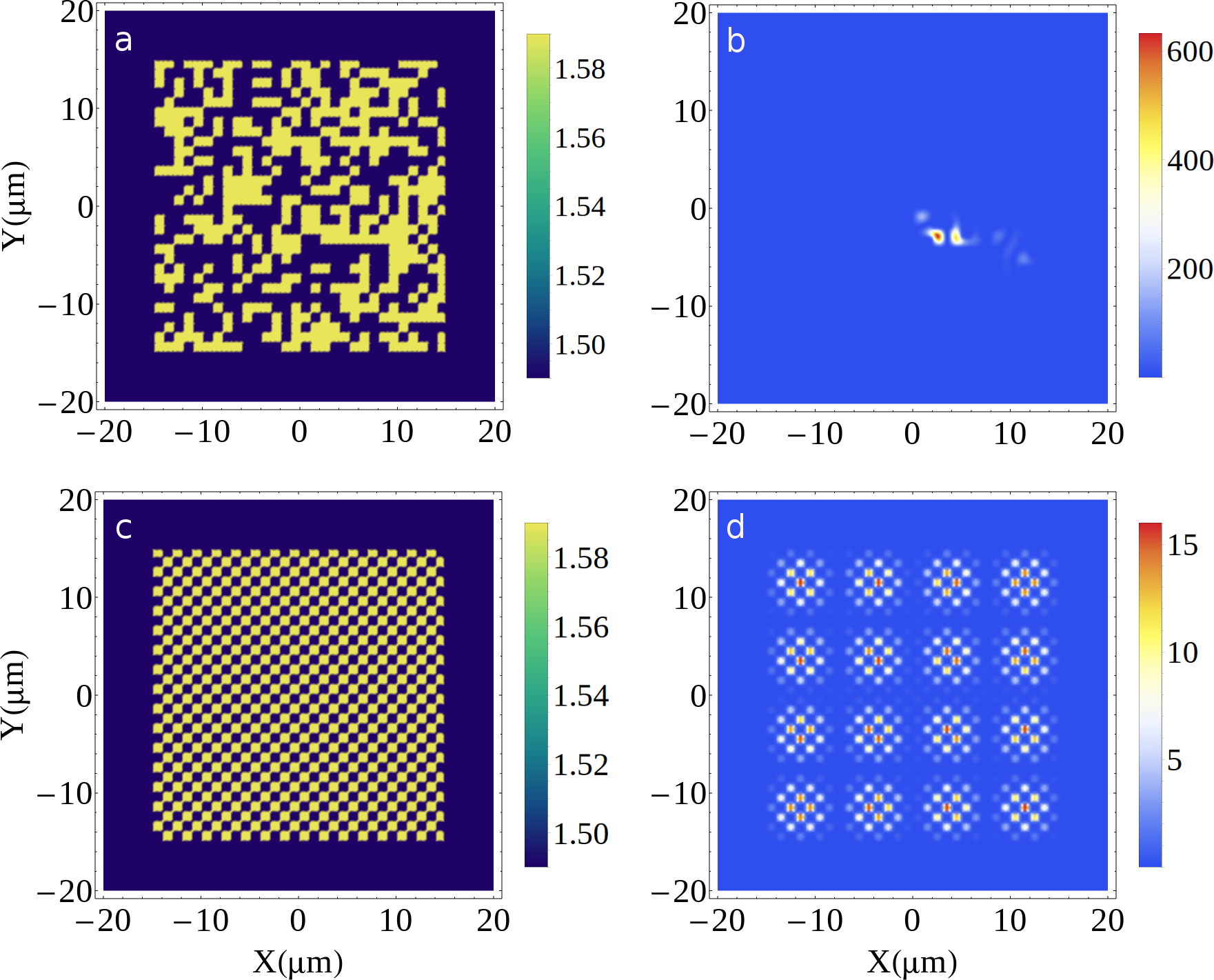
Figure 1: Sample refractive index profiles of (a) disordered and (c) ordered optical fiber with an arbitrarily selected square cross section. (b), and (d) represent the typical calculated modes for the index profiles in (a), and (c), respectively. For a disordered optical fiber modes are transversely localized as opposed to the ordered fiber where the mode covers the entire cross section of the fiber.

In the rest of the paper, we will explore MA-PDF curves for TALOFs. For each MA-PDF curve, we have calculated all the guided modes (typically tens of thousands of modes) for at least ten individual realizations of the specific disordered configuration under study in order to take into account the statistical nature of the disordered fiber. We should emphasize that for a device-level application of TALOF, a strong disorder is desirable to ensure self-averaging and therefore, reliable performance of a single disordered device realization Karbasi et al. (2012a, 2014).

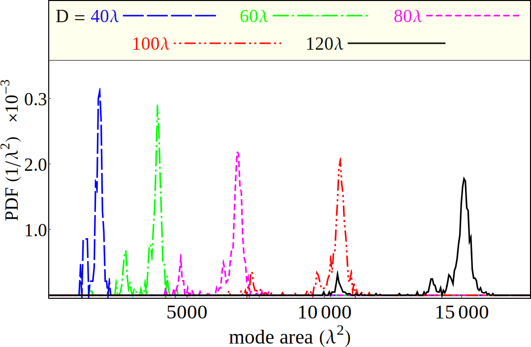
Figure 2: Mode-area PDF of a transversely periodic fiber formed by $N\times N$ number of unit cells for N = 20, 30, 40, 50, and 60 where the unit cell is a square of $2\lambda$ side-width. The average mode area of the transversely periodic fiber is solely determined by the transverse size of the fiber.

In the absence of disorder, guided modes of a conventional optical fiber are extended over the entire transverse dimensions of the fiber, an example of which is shown in Fig. 1(d); total internal reflection caused by the index step formed at the interface between the fiber core and cladding is responsible for the overall transverse wave confinement as it propagates freely in the third longitudinal direction. Therefore, the average transverse size of the guided modes scales proportionally to the cross-sectional area of the fiber. Figure 2 shows the MA-PDF of transversely periodic fibers with $N\times N$ unit cells in the core. In our notation, unless otherwise specified, each unit cell is a square with a side-width of $d=2\lambda$, so the area of each unit cell is $a=4\lambda^{2}$. Therefore, the fiber core width of $D=$ 40, 60, 80, 100, and 120$\lambda$ in Fig. 2 correspond to $N=$ 20, 30, 40, 50, and 60 unit cells in each direction. $n_{1}=1.58$, and $n_{2}=1.59$ are used in Fig. 2 so the index step in the core of the fiber equals to ${\Delta n_{\rm core}}=n_{2}-n_{1}=0.01$. The horizontal axis is in units of $\lambda^{2}$ and the vertical axis is in units of $1/\lambda^{2}$ such that the total area under the PDF integrates to unity. The thickness of the cladding is $t=5\lambda$ around the periodic core of the fiber and its refractive index $n_{c}$ is chosen to be equal to the lower core index $n_{1}$. Figure 2 indicates that for the periodic fibers, the transverse size of the modes is solely determined by the size of the fiber core. Therefore, the peak of the MA-PDF shifts towards larger values of mode area as the fiber becomes wider.

For a disordered optical fiber, the scaling characteristics of the MA-PDF with respect to the transverse dimensions of the fiber are completely different from the periodic case. Disorder-induced TAL localizes most of the guided modes across the transverse structure of the disordered fiber and each mode provides a narrow guiding channel Ruocco et al. (2017).

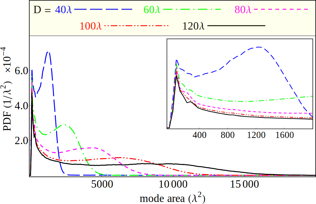
Figure 3: Mode-area PDF of a disordered fiber exactly the same as Fig. 2, except in the fact that refractive index of each unit cell is randomly chosen from the $(n_{1},n_{2})$ pair. The MA-PDF clearly represents presence of localized modes at $\sim 75\lambda^{2}$ and a long tail representative of guided extended modes. Moreover, saturation of the PDF in the highly localized region beyond $D_{\rm sat}\approx 100\lambda$ is clear in this figure. The inset is the magnified version of the localized peaks of the PDFs.

Figure 3 shows the MA-PDF for a TALOF where all parameters involved in the disordered structure are exactly the same as Fig. 2, except in the fact that refractive index of each unit cell is randomly chosen from the $(n_{1},n_{2})$ pair with an equal probability. The MA-PDF shows a localized peak at a value less than $\approx 75\lambda^{2}$; therefore, the modes appear to be highly localized. The long tail of the PDF represents the guided extended modes that cover a large portion of the fiber cross section.

In Fig. 3, the MA-PDF broadens as the number of cells is increased. The localized mode section below 1000$\lambda^{2}$ converges rapidly as a function of $D$ and remains nearly unchanged beyond $D_{\rm sat}\approx 100\lambda$. The tail of the distribution also converges albeit more slowly where the hump which is an artifact of the boundary gradually disappears and is replaced by a long decaying tail Abaie and Mafi (2016).

Convergence of MA-PDF beyond a critical number of cells indicates that $D_{\rm sat}$ can be considered as the effective transverse size of the disordered fiber beyond which the impact of the boundary on the localization properties is considerably reduced. Moreover, a disordered fiber with $D_{\rm sat}\approx 100\lambda$ can fully represent the behavior of a much wider fiber, hence significantly reducing the computational cost of simulating real-sized fibers. In order to see the saturation behavior of the MA-PDF more clearly, the inset shows a magnified version of the MA-PDFs, which is zoomed-in around smaller mode-area values.

The results shown in Fig. 3 are related to a disordered fiber with an index difference of ${\Delta n_{\rm core}}=0.01$. If ${\Delta n_{\rm core}}$ is increased, the stronger transverse scattering must result in a stronger transverse localization and therefore smaller mode area values in the MA-PDF curve. A stronger transverse scattering is achieved by increasing the value of the index difference to ${\Delta n_{\rm core}}=0.1$ ($n_{1}=1.49$ and $n_{2}=1.59$). These values of $n_{1}$ and $n_{2}$ are chosen in accordance to the materials used in Ref. Karbasi et al. (2012a) and the result is represented in Fig. 4. The peak values of MA-PDF curves occur at smaller mode area values ($\sim 15\lambda^{2}$), indicative of a stronger transverse localization. Moreover, the peaks are considerably narrower in Fig. 4 compared with those in Fig. 3, because a stronger disorder also reduces the variance around the mean as discussed in Ref. Karbasi et al. (2012b), hence resulting in a more uniform imaging PSF. Also, for the larger value of ${\Delta n_{\rm core}}=0.1$, the convergence of the PDF occurs for considerably smaller disordered fibers ($D_{\rm sat}\approx 60\lambda$).

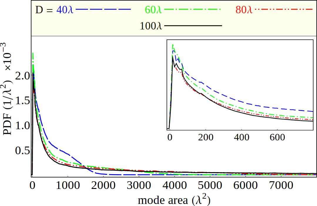
Figure 4: Mode-area PDF of a disordered fiber with exactly the same configuration as Fig. 3 except for ${\Delta n_{\rm core}}=0.1$. Larger refractive index contrast in the disordered structure makes the PDF much narrower due to a much stronger localization. Inset is the magnified version of the localized peaks of the PDFs . Saturation of the PDF beyond $D_{\rm sat}\approx 60\lambda$ is clear in this figure.

As an example for the utility of the concepts introduced here, we can tackle the important question of what the optimum value of the transverse scatterer size is to obtain the smallest imaging PSF. In the previous figures, it was assumed that the unit cells in the disordered core of the fiber are squares with a side-width of $d=2\lambda$, in accordance to the TALOF reported in Ref. Karbasi et al. (2012a). Conceptually, one can imagine that if $d\ll\lambda$, the wavelength is much larger than the scatterer size and the medium appears as homogeneous to the wave. For $d\gg\lambda$, the system will be in the geometrical optics limit. In either case, one expects a weak localization effect; therefore, $d\sim\lambda$ is desired for maximum localization and the exact optimum value can be calculated from the relevant MA-PDF.

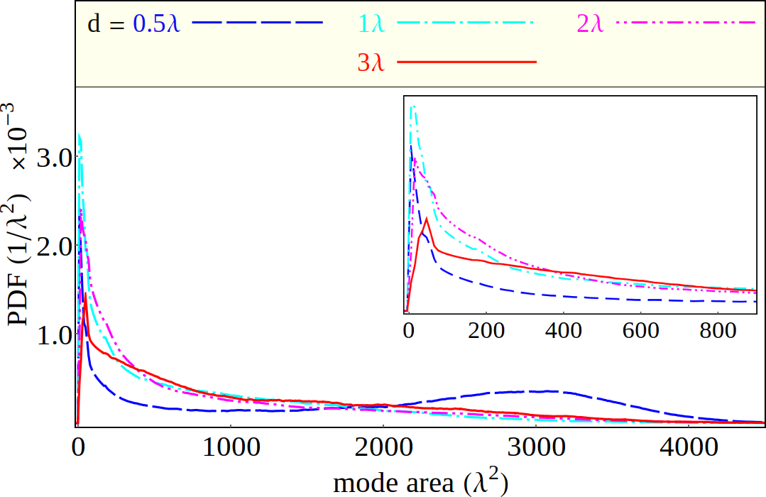
Figure 5: PDF of disordered fibers with $D=60\lambda$, ${\Delta n_{\rm core}=0.1}$, and $d=\lambda/2,~{}\lambda,~{}2\lambda$, and $3\lambda$. $d\sim\lambda$ is desired for maximum localization strength.

In order to find the impact of the cell size, we compute in Fig. 5 the MA-PDF curves in the saturation regime for TALOFs with several different values of cell size: $d=\lambda/2$, $\lambda$, $2\lambda$, and $3\lambda$. In all cases, we assume that ${\Delta n_{\rm core}=0.1}$ and the fiber core width is $60\lambda$. The results seem consistent with the discussion above, where $d\sim\lambda$ is the desired vaue for maximum localization. Of course, the exact choice of the value of $d$ depends on a target function that must be calculated in a specific imaging scenario. It is not just the localized modes that matter for imaging applications because the presence of the extended modes can also reduce the contrast Karbasi et al. (2013); therefore, the optimization function must consider both the size of the PSF as well as the contrast for the specific scenario. Figure 5 clearly shows that for a given transverse size, the MA-PDF in the extended mode region looks different for different values of $d$.

It is also important to point out that these results are not in contradiction with those reported in Ref. Schirmacher et al. (2017) where no dependence of the observed localization radii is found on the light wavelength. The results of Ref. Schirmacher et al. (2017) are for averages of localization radii in the limit of infinite transverse fiber dimensions. How the MA-PDF can be averaged over the mode area in order to obtain the average localization radius of Ref. Schirmacher et al. (2017) is beyond the scope of the present paper and will be dealt with in a future publication.

In conclusion, a detailed statistical analysis based on MA-PDF is suggested as a powerful tool to study TAL of light, especially in disordered optical fibers. It is shown that the MA-PDF can be reliably computed form structures considerably smaller than those used in experiments, hence substantially reducing the computational cost to study TAL. The information contained in an MA-PDF can be used to study and optimizes devices that operate based on TAL, e.g. in endoscopic image transport fibers Karbasi et al. (2014); Zhao et al. (2017) and directional fiber-based random lasers Abaie et al. (2017). The authors would like to point out that low-amplitude high-frequency oscillations of the MA-PDF cuvres presented in this paper have been smoothed out for clearer presentation without compromising the results; however, original data can be obtained from the authors upon request.

The authors are thankful to the UNM Center for Advanced Research Computing (CARC) for providing access to computational resources used in this work.

References

- Anderson (1958) P. W. Anderson, Phys. Rev. 109, 1492 (1958).
- Abrahams (2010) E. Abrahams, 50 Years of Anderson Localization (World Scientific, Singapore, 2010).
- Mordechai Segev and Christodoulides (2013) Y. S. Mordechai Segev and D. N. Christodoulides, Nature Photonics 7, 197 (2013).
- Weaver (1990) R. Weaver, Wave Motion 12, 129 (1990).
- Graham et al. (1990) I. S. Graham, L. Piché, and M. Grant, Phys. Rev. Lett. 64, 3135 (1990).
- Dalichaouch et al. (1991) R. Dalichaouch, J. Armstrong, S. Schultz, P. Platzman, and S. McCall, (1991).
- John (1984) S. John, Phys. Rev. Lett. 53, 2169 (1984).
- John (1987) S. John, Phys. Rev. Lett. 58, 2486 (1987).
- John (1991) S. John, Phys. Today 44, 32 (1991).
- Anderson (1985) P. W. Anderson, Philosophical Magazine Part B 52, 505 (1985).
- Lagendijk et al. (2009) A. Lagendijk, B. van Tiggelen, and D. S. Wiersma, Physics Today 62, 24 (2009).
- Hu et al. (2008) H. Hu, A. Strybulevych, J. H. Page, S. E. Skipetrov, and B. A. van Tiggelen, Nat Phys 4, 945 (2008).
- Chabanov and Genack (2000) S. M. Chabanov, A. A. and A. Z. Genack, Nature 404, 850 (2000).
- Billy et al. (2008) J. Billy, V. Josse, Z. Zuo, A. Bernard, B. Hambrecht, P. Lugan, D. Clément, L. Sanchez-Palencia, P. Bouyer, and A. Aspect, Nature 453, 891 (2008).
- Lahini et al. (2010) Y. Lahini, Y. Bromberg, D. N. Christodoulides, and Y. Silberberg, Phys. Rev. Lett. 105, 163905 (2010).
- Lahini et al. (2011) Y. Lahini, Y. Bromberg, Y. Shechtman, A. Szameit, D. N. Christodoulides, R. Morandotti, and Y. Silberberg, Phys. Rev. A 84, 041806 (2011).
- Abouraddy et al. (2012) A. F. Abouraddy, G. Di Giuseppe, D. N. Christodoulides, and B. E. A. Saleh, Phys. Rev. A 86, 040302 (2012).
- Thompson et al. (2010) C. Thompson, G. Vemuri, and G. S. Agarwal, Phys. Rev. A 82, 053805 (2010).
- Skipetrov and Sokolov (2014) S. E. Skipetrov and I. M. Sokolov, Phys. Rev. Lett. 112, 023905 (2014).
- Schirmacher et al. (2017) W. Schirmacher, B. Abaie, A. Mafi, G. Ruocco, and M. Leonetti, arXiv preprint arXiv:1705.03886 (2017).
- Abdullaev and Abdullaev (1980) S. S. Abdullaev and F. K. Abdullaev, Radiofizika 23, 766 (1980).
- De Raedt et al. (1989) H. De Raedt, A. Lagendijk, and P. de Vries, Phys. Rev. Lett. 62, 47 (1989).
- Schwartz et al. (2007) T. Schwartz, G. Bartal, S. Fishman, and M. Segev, Nature 446, 52 (2007).
- Lahini et al. (2008) Y. Lahini, A. Avidan, F. Pozzi, M. Sorel, R. Morandotti, D. N. Christodoulides, and Y. Silberberg, Phys. Rev. Lett. 100, 013906 (2008).
- Martin et al. (2011) L. Martin, G. D. Giuseppe, A. Perez-Leija, R. Keil, F. Dreisow, M. Heinrich, S. Nolte, A. Szameit, A. F. Abouraddy, D. N. Christodoulides, and B. E. A. Saleh, Opt. Express 19, 13636 (2011).
- Karbasi et al. (2012a) S. Karbasi, C. R. Mirr, P. G. Yarandi, R. J. Frazier, K. W. Koch, and A. Mafi, Opt. Lett. 37, 2304 (2012a).
- Karbasi et al. (2012b) S. Karbasi, C. R. Mirr, R. J. Frazier, P. G. Yarandi, K. W. Koch, and A. Mafi, Opt. Express 20, 18692 (2012b).
- Karbasi et al. (2012c) S. Karbasi, T. Hawkins, J. Ballato, K. W. Koch, and A. Mafi, Opt. Mater. Express 2, 1496 (2012c).
- Mafi (2015) A. Mafi, Adv. Opt. Photon. 7, 459 (2015).
- Abaie et al. (2016) B. Abaie, S. R. Hosseini, S. Karbasi, and A. Mafi, Optics Communications 365, 208 (2016).
- Abaie and Mafi (2016) B. Abaie and A. Mafi, Phys. Rev. B 94, 064201 (2016).
- Karbasi et al. (2014) S. Karbasi, R. J. Frazier, K. W. Koch, T. Hawkins, J. Ballato, and A. Mafi, Nat Commun 5 (2014).
- COMSOL-Multiphysics (2016) COMSOL-Multiphysics, Wave Optics Module (2016).
- Ruocco et al. (2017) G. Ruocco, B. Abaie, W. Schirmacher, A. Mafi, and M. Leonetti, Nature Communications 8 (2017).
- Karbasi et al. (2013) S. Karbasi, K. W. Koch, and A. Mafi, Optics Communications 311, 72 (2013).
- Zhao et al. (2017) J. Zhao, J. E. Antonio-Lopez, R. A. Correa, A. Mafi, M. Windeck, and A. Schülzgen, in Conference on Lasers and Electro-Optics (Optical Society of America, 2017) p. JTu5A.91.
- Abaie et al. (2017) B. Abaie, E. Mobini, S. Karbasi, T. Hawkins, J. Ballato, and A. Mafi, Light: Science & Applications 6 (2017).