The benefits of a near detector for JUNO

Abstract

It has been proposed to determine the mass hierarchy of neutrinos by exploiting the beat between the oscillation frequencies corresponding to the two neutrino mass squared differences. JUNO is based on this concept and uses a large liquid scintillator detector at a distance of 53 km from a powerful nuclear reactor complex. We argue that the micro-structure present in antineutrino fluxes from nuclear reactors makes it essential to experimentally determine a reference spectrum with an energy resolution very similar to the one of JUNO.

The Jiangmen Underground Neutrino Observatory (JUNO) comprises a 20 kt liquid scintillator detector with a broad physics program An et al. (2016a). One of the key physics goals of JUNO is the determination of the so-called mass hierarchy of neutrinos, that is, whether the third mass eigenstate is the lightest (inverted hierarchy, IH) or heaviest (normal hierarchy, NH) without having to rely on matter effects: with an appropriate choice of experimental parameters, it is possible to simultaneously be sensitive to oscillations corresponding to the two mass squared differences ${\Delta m^{2}_{31}}\simeq 2.5\times 10^{-3}\,\mathrm{eV}^{2}$ and ${\Delta m^{2}_{21}}\simeq 7.4\times 10^{-5}\,\mathrm{eV}^{2}$ Patrignani et al. (2016). In this case, also, the beat frequency between the two oscillations will be present, and whether this beat frequency is larger or smaller than the main oscillation driven by ${\Delta m^{2}_{31}}$ is a direct measure of the mass hierarchy Petcov and Piai (2002); the amplitude of the beat is given by $\sin^{2}2\theta_{13}$. The relative difference between the beat frequency and main oscillation is of the order ${\Delta m^{2}_{21}}/{\Delta m^{2}_{31}}\simeq 1/30$, and thus an energy resolution of approximately $3\%$ is required.

JUNO will detect reactor antineutrinos via inverse beta decay (IBD) and is situated 53 km from both the Yangjiang and Taishan nuclear power plants, the distance being carefully chosen to fulfill above conditions and to optimize the mass hierarchy sensitivity. Neutrino energy reconstruction in IBD, $\bar{\nu}_{e}+p\rightarrow n+e^{+}$, is relatively straightforward; the visible energy of the positron, $E_{e^{+}}$, is related to the neutrino energy $E_{\nu}$ via

$$E_{\nu}=E_{e^{+}}+(m_{n}-m_{p}-m_{e})\,,$$ (1)

neglecting the kinetic energy of the outgoing neutron, which, for the neutrino energies in question, is an excellent approximation. The energy deposited by the positron in the scintillator is converted to light, and the energy resolution is determined by photon counting statistics and, to first order, scales as $1/\sqrt{E_{e^{+}}}$.

Attaining the requisite $3\%$ energy resolution is a challenge in itself, but, given the relatively small size of the effect, the question of systematic uncertainties needs to be addressed. There are three main types of systematics for this measurement: uncertainty in ${\Delta m^{2}_{31}}$, i.e. uncertainty about the main oscillation frequency; uncertainty in the detector energy response, e.g. a shift of the energy scale has the the same effect as a change in ${\Delta m^{2}_{31}}$; reactor antineutrino flux uncertainties, since one is searching for a high-frequency component in the Fourier spectrum, and any high-frequency components in the flux can lead to confusion. All of these have been discussed in various combinations in the literature, and, in particular, the JUNO collaboration is clearly aware of them An et al. (2016a).

The goal of this letter is to highlight the impact of one source of uncertainty which is recognized but may have been underestimated: the reactor antineutrino flux. For all the systematic effects except the ${\Delta m^{2}_{31}}$ uncertainty, some type of parameterization or implementation in the analysis has to be found. We argue, here, that the parameterizations used previously to account for the reactor flux uncertainties are not capturing the relevant degrees of uncertainty; in other words, some of the known unknowns are not accounted for. Using a more physical model for the reactor flux uncertainties, a large reduction of sensitivity to the mass hierarchy results. This problem can be completely resolved by using a reference reactor antineutrino spectrum measured with a similar energy resolution as the JUNO detector. We demonstrate this by including a near detector in the simulation.

Reactor antineutrino fluxes have taken center stage as a research subject of their own since a series of papers Mueller et al. (2011); Huber (2011) in 2011 (Huber+Mueller model), which led to a revision of the flux models, giving rise to the reactor antineutrino anomaly (RAA) Mention et al. (2011). Antineutrinos from reactors are not made directly in the fission process; instead, they arise from the beta decays of neutron-rich fission products. There are roughly $10^{3}$ isotopes with about $10^{4}$ individual beta decay branches which would have to be known with good accuracy to compute the antineutrino flux with percent level errors. This knowledge does not exist, and thus measurements of the total beta decay spectrum from fission fragments Von Feilitzsch et al. (1982); Schreckenbach et al. (1985); Hahn et al. (1989) are used as a basis for unfolding the antineutrino spectrum. The 2011 papers have triggered significant follow-up work, and this led to the understanding that first forbidden non-unique beta decays, which make up anywhere between 20-30% of all antineutrinos relevant for IBD, and their higher-order corrections, like weak magnetism, are dominating the error budget and likely exceed the estimates Mueller et al. (2011); Huber (2011), a point driven home by the observation of a 5 MeV bump in the measured antineutrino spectrum relative to predictions, see for instance the Daya Bay result An et al. (2017); for recent reviews on this topic, see Refs. Huber (2016); Hayes and Vogel (2016).

As explained, a direct calculation of antineutrino fluxes is not feasible; nonetheless, these direct or a priori calculations allow some significant insight into the energy structure of the antineutrino spectrum without being obstructed by real-world detector effects, see for instance Ref. Fallot et al. (2012). In Fig. 3 of Ref. Dwyer and Langford (2015), it is highlighted that there is significant micro-structure in the antineutrino spectrum at the 50–100 keV scale. This sawtooth shape arises because, in a single beta decay, there is a finite probability to emit an antineutrino with an energy corresponding to the entire available $Q^{2}$ of the transition due to the Coulomb correction experienced by the outgoing electron. Adding a large number of these, then, results in the sawtooth pattern also visible in Fig. 1. In Ref. Dwyer and Langford (2015), it is also shown that, once this sawtooth spectrum is convoluted with a detector energy resolution typical for current reactor neutrino experiments, an entirely smooth spectrum results.

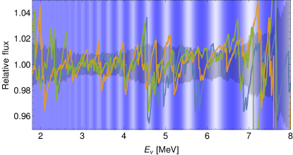
Figure 1: Shown are three synthetic antineutrino spectra relative to the antineutrino spectrum predicted from the ILL data Mueller et al. (2011); Huber (2011) (Huber+Mueller model) normalized to the same total IBD event rate. The gray shaded horizontal band shows the standard deviation of the whole population of synthetic spectra. For illustration, the vertical bands indicate the oscillation arising from ${\Delta m^{2}_{31}}$ at a distance $L=53$ km smeared with an energy resolution of $3\%/\sqrt{E}$.

A priori calculations account for about 80-90% of all beta decays and, thus, reproduce the total beta spectrum as measured by the ILL experiments to about the same degree Fallot et al. (2012). Therefore, there is no reason to expect that the specific energy micro-structure derived from any of these calculations is the actual one: the specific location and size of each sawtooth is likely wrong; the distribution of locations and sizes, on the other hand, will be close to the true one. For the following, we use a model based on thermal neutron fission yields of ²³⁵U, ²³⁹Pu, and ²⁴¹Pu from the JEFF database, version 3.1.1 jef , and the fast neutron fission yield of ²³⁸U from ENDF-349 England and Rider (1994). We use the beta decay information contained in the Evaluated Nuclear Structure Data File (ENSDF) database, version VI ens , and the neutrino spectrum is computed following the prescription in Ref. Huber (2011). We use this information on fission yields and beta decays to construct a probability density function $p(Q,a)$ for the $Q$-value and amplitude $a$ for each beta decay branch. We then draw at random pairs of values for $Q,a$ and compute the resulting antineutrino spectrum; we stop adding more pairs as soon as we have the same number of antineutrinos above IBD threshold as in the Huber+Mueller model. The resulting antineutrino spectrum is then normalized to the same IBD rate as obtained from the Huber+Mueller model and reweighted to represent the shape of the Huber+Mueller flux at an energy resolution of $8\%/\sqrt{E}$. We repeat the procedure 1000 times to obtain a population of synthetic antineutrino spectra which all correspond to a very similar spectrum at $8\%/\sqrt{E}$ resolution. The results are shown in Fig. 1, where we show the resulting distribution for each energy bin relative to its mean (the Huber+Mueller prediction), and we also show three examples of a synthetic spectrum. For comparison, the relevant oscillation is overlayed; it is apparent that much of the structure in the synthetic spectrum is at a similar frequency and amplitude as the effect sought after in JUNO. This indicates that the strategy outlined in Ref. An et al. (2016a) to deal with the reactor flux uncertainty, namely to use the Daya Bay measured spectrum as reference spectrum is fraught with difficulty: the Daya Bay spectrum has been measured with an energy resolution of approximately $8\%/\sqrt{E}$ whereas for JUNO the spectrum at $3\%/\sqrt{E}$ is needed.

The question now is: what energy resolution does the reference spectrum need to be measured with, and what other detector effects could intervene? The effect of having a second detector (near detector) in the hierarchy determination has been discussed in more general terms in Refs. Ciuffoli et al. (2014); Capozzi et al. (2015); Wang et al. (2016). Specifically, we investigate the non-linearity of the energy response as a potential issue in comparing the data from two detectors. The Daya Bay detectors are precision instruments, and their success has inspired the design for JUNO, therefore it makes sense to use them as a proxy for the energy response. For the Daya Bay detectors, the energy response to positrons is non-linear with the main effect happening below the $4\,\text{MeV}$. This effect is attributed to ionization quenching of scintillation light and Cerenkov light production and peculiarities of the electronics An et al. (2014).

To include non-linear effects in the reconstruction of the positron energy one can parameterize the effect as a linear combination of functions that are powers of energy, generalizing the linear scaling Li et al. (2013); Capozzi et al. (2015):

$$\frac{E_{\text{rec}}}{E}=1+\sum_{k=0}^{n}\alpha_{k}E^{k}\equiv 1+\delta_{\text{scal}}(E).$$ (2)

For $k=0$, and with only $\alpha_{0}\neq 0$, one obtains the linear case (linear scaling). Therefore, to include non-linear effects, $\alpha_{k}\neq 0$, one needs to include higher energy powers in Eq. (2). Even though this approach is conceptually simple, it does offer neither a physical condition when to stop the series nor allows to set the size and to understand the physical meaning of the non-linear coefficients.

Assuming the energy response of the JUNO detector will be similar to the one of Daya Bay Ref. An et al. (2016b), it is possible to estimate the remaining error $S_{\text{scal}}(E)$ after the non-linear correction has been applied as a relative deviation from the nominal model. This procedure was implemented in Ref. Li et al. (2013); Capozzi et al. (2015), where the error envelope $S_{\text{scal}}(E)$ is taken from the reported detector energy response function in Ref. An et al. (2016b). The largest energy scale error is around $2\%$ in the low energy region; for most of the energy range the error is below $1\%$; we follow the procedure outlined in Ref. Capozzi et al. (2015).

To include the effect of the remaining error after the non-linear detector energy response correction in the analysis, we have generalized the algorithm used to account for the linear scaling in GLoBES  Huber et al. (2003). Notice that in principle the individual $\alpha_{k}$ coefficients can be arbitrarily large, except for $|\alpha_{0}|\lesssim 2\%$, since they have no direct physical meaning, and, at any energy, only the sum of all terms is constrained by the Daya Bay model. This is clearly a shortcoming of the parameterization given in Eq. (2). The overall Daya Bay constraint is implemented as a penalty on the $\chi^{2}$-function Capozzi et al. (2015):

$$\chi^{2}_{\text{scal}}=\text{max}_{E}\left|\frac{\delta_{\text{scal}}(E)}{S_{\text{ scal}}(E)}\right|^{2}.$$ (3)

After implementing the penalty in Eq. (3) in the JUNO simulation, we find that the $\chi^{2}$-function becomes somewhat wider as a function of ${\Delta m^{2}_{31}}$, indicating as mentioned previously, the similarity between a linear energy scale uncertainty and a less precise input on ${\Delta m^{2}_{31}}$. We also find that the result practically does not change for $k=2$, and thus there is no reason to go beyond $k=2$. For $k=2$ the sensitivity to the mass hierarchy is decreased by $\sim 1.23$ $\Delta\chi^{2}$ units, taking the case of the linear scaling as reference ($\Delta\chi^{2}_{\text{min}}\simeq 23$), which is compatible with the result in Ref. Capozzi et al. (2015). Also, a pull on $\Delta m_{31}^{2}$ has to be included Li et al. (2013), since its effect (within the current errors) can mimic the non-linear effects we are introducing, as was pointed out previously Qian et al. (2013); Ciuffoli et al. (2014).

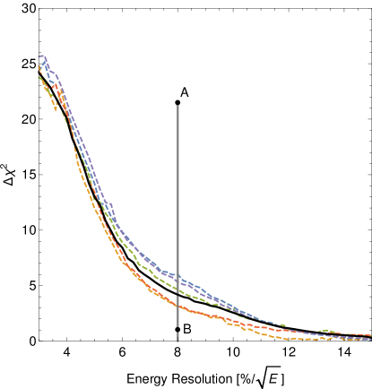
Figure 2: $\Delta\chi^{2}$ between normal and inverted hierarchy (assuming normal hierarchy to be true) for a JUNO-like experiment employing a reference measurement of the reactor spectrum with an energy resolution given by the abscissa. The solid line assumes that the same spectrum is used to generate and fit the data, whereas, for the dashed lines, we use a random synthetic spectrum to generate the data and fit the data with Huber+Mueller model. The points labeled A and B, show the result obtained by using the actually measured antineutrino spectrum from Daya Bay An et al. (2017): for point A we are using one nuisance parameter per Daya Bay bin and for point B we are using one nuisance parameter in each of 100 bins.

Now, we can address how well a reference spectrum needs to be measured in terms of energy resolution. To this end, we set up a model with a 5 ton near detector at a distance of 0.5 km, which yields approximately $1.6\times 10^{5}$ events per year. For the far detector, we assume 20 kt fiducial mass at a distance of 53 km. For both detectors, we use the non-linearity model described above with $k=2$, and the $\alpha_{k}$ are varied independently for near and far detectors, reflecting the assumption that the $\alpha$’s are constrained by the calibration systems of each detector independently. We use 100 bins to compute the spectrum prior to applying the energy resolution function, and for each bin, we introduce a nuisance parameter, which is fully correlated between near and far detectors, but otherwise unconstrained. This corresponds to a flux model where no prior knowledge on fluxes is assumed except that the energy scale of variations can be as small as about 50 keV. We argued in the introduction that the relevant degrees of uncertainty in the flux lie in this micro-structure, and, locally, deviations can be quite large, see Fig. 1, whereas the deviation of the mean is quite small. Finally, we use $3\%/\sqrt{E}$ as energy resolution for the far detector and vary the resolution of the near detector, with the result shown as solid line in Fig. 2. For the solid line, we use the same flux model (Huber+Mueller) to generate the data and fit it. For the dashed lines, we use a synthetic spectrum, drawn at random from the population, to generate the data and attempt to fit it with the Huber+Mueller model: the result is close to the solid line. We conclude that, without a dedicated near detector, the sensivity accounting for realistic flux errors decrease from $\Delta\chi^{2}\simeq 22$ to $\Delta\chi^{2}\simeq 4$; whereas, with a decicated near detector, the sensitivity may improve beyond the original one, since all flux uncertainties are eliminated.

For comparsion, in Fig. 2 we also show the $\chi^{2}$-values obtained by using instead of a near detector the actually measured Daya Bay antineutrino spectrum and its full covariance matrix An et al. (2017). Point A corresponds to the case where we allow one nuisance parameter for each Daya Bay energy bin of approximately 250 keV width and find indeed, that the Daya Bay data would fully eliminate the effect of flux uncertainties. Point B, however, is computed with one nuisance paramater for each of 100 bins corresponding to the case of significant micro-structure in the antineutrino flux. Clearly, in that case the Daya Bay measurement is insufficient to eliminate this systematic. Note, that point B lies below the black line, which is based on a idealized near detector, because of real-world detector effects which result in significant spectrum uncertainties in the Daya Bay data for very low and very high antineutrino energies.

In summary, we made the argument that antineutrino reactor fluxes have a micro-structure at the 50 keV level which is similar to the mass hierarchy signal in experiments like JUNO. We performed a careful study of the impact of non-linearities in the energy response and find that, overall, they have a limited impact on these experiments. We show that a reference measurement of the antineutrino spectrum with an energy resolution very similar to the far detector is needed to exclude any sensitivity reduction due to the unknown micro-structure of the antineutrino flux. For simplicity, we implement a near detector, which, for a real experiment, has the added benefit of providing information on the actual running conditions of the reactor(s), and thus helps to eliminate any systematic uncertainties which otherwise could arise. However, a reference measurement performed at a different time and/or different reactor, for the purposes of this study, would be acceptable as long as the energy resolution is similar to the one of the far detector.