Historical Document Image Segmentation with LDA-Initialized Deep Neural Networks

Abstract.

In this paper, we present a novel approach to perform deep neural networks layer-wise weight initialization using Linear Discriminant Analysis (LDA). Typically, the weights of a deep neural network are initialized with: random values, greedy layer-wise pre-training (usually as Deep Belief Network or as auto-encoder) or by re-using the layers from another network (transfer learning). Hence, many training epochs are needed before meaningful weights are learned, or a rather similar dataset is required for seeding a fine-tuning of transfer learning. In this paper, we describe how to turn an LDA into either a neural layer or a classification layer. We analyze the initialization technique on historical documents. First, we show that an LDA-based initialization is quick and leads to a very stable initialization. Furthermore, for the task of layout analysis at pixel level, we investigate the effectiveness of LDA-based initialization and show that it outperforms state-of-the-art random weight initialization methods.

1. Introduction

Very Deep Neural Network (DNN) are now widely used in machine learning for solving tasks in various domains.

Although artificial neurons have been around for a long time (McCulloch and Pitts, 1943), the depth of commonly used artificial neural networks has started to increase significantly only for roughly 15 years(Goodfellow et al., 2016). This is due to both: the coming back of layer-wise training methods(Ballard, 1987) and the higher computational power available to researchers.

Historical Document Image Analysis (Dia) is an example of a domain where DNN have been successfully applied recently. As historical documents can be quite diverse, simple networks with few inputs usually lead to poor results, so large networks have to be used. The diversity of the documents has several origins: different degradations (e.g ink fading or stains), complexity and variability of the layouts, overlapping of contents, writing styles, bleed-through, etc.

Because of their success, a lot of resources have been invested into research and development of DNN. However, they still suffer from two major drawbacks. The first is that, despite the computational power of new processors and GPUs, the training of DNN still takes some time. Especially for large networks, the training time becomes a crucial issue, not only because there are more weights to use in the computations, but also because more training epochs are required for the weights to converge. The second drawback is that initializing the weights of DNN with random values implies that different networks will find different local error minima.

In our previous work (Seuret et al., 2017) we proposed to initialize a Convolutional Neural Network (CNN) layer-wise with Principal Component Analysis (PCA) instead of random initialization. We also have shown how features which are good for one task do not necessarily generalize well to other tasks (Alberti et al., 2017c, b). Per extension, we argue that features obtained by maximizing the variance of the input data — which is what PCA features do — might not be the optimal ones for performing classification tasks. To this end, we investigate the performances of initializing a CNN layer-wise with a goal oriented (supervised) algorithm such as LDA by performing layout analysis at the pixel level on historical documents.

Contribution

In this paper, we present a novel initialization method based on LDA which allows to quickly initialize the weights of a CNN layer-wise with data-based values. We show that such initialization is very stable, converge faster and to better performances when compared with the same architecture initialized with random weights. Additionally, even before the fine-tuning a network initialized with LDA exhibits noticeable results for classification task.

Related work

Follows a brief review of literature relevant for this work.

Random Neural Network Initialization

There are currently three main trends for neural network initialization: layer-wise unsupervised pre-training (Ballard, 1987; Hinton et al., 2006), transfer learning (Caruana, 1998) or random initial initial weights (Bottou, 1988). Random initialization is fast and simple to implement. The most used approach is to initialize weights of a neuron in $\left[-\sqrt{n},\sqrt{n}\right]$, where $n$ is the number of inputs of the neuron.

PCA Neural Network Initialization

In our previous work (Seuret et al., 2017) we successfully initialized a CNN layer-wise with PCA. In this work, we introduced a mathematical framework for generating Convolutional Auto-Encoder (CAE) out of the PCA, taking into account the bias of neural layers, and provide a deep analysis of the behavior of PCA-initialized networks – both for CAE and CNN – with a focus on historical document images. Krähenbühl et al. (Krähenbühl, Philipp and Doersch, Carl and Donahue, Jeff and Darrell, Trevor, 2015) conducted a similar, but independent, research in which, while investigating data-dependent initialization, used PCA matrices as neural layer initial weights. They however mainly focus on K-means initialization and do not investigate deeply PCA initialization.

Linear Discriminant Analysis in Neural Networks:

The link between Neural Networks and LDA has been investigated by many authors. Among them, there are Webb and Lowe (Webb and Lowe, 1990) who have shown that the output of hidden layers of multi-layer perceptrons are maximizing the network discriminant function, explicitly performing a non-linear transformation of the data into a space in which the classes may be more easily separated. Demir and Ozmehmet (Demir and Ozmehmet, 2005) presented an online local learning algorithms for updating LDA features incrementally using error-correcting and the Hebbian learning rules. Recently, Dorfer at al. (Matthias et al., 2015) have shown how to learn linearly separable latent representations in an end-to-end fashion on a DNN. To the best of our knowledge, there have been no attempts to use LDA for direct NN initialization.

2. Mathematical formulation

In this section we explain the general idea of the Linear Discriminant Analysis and then give the mathematical formulation for using it both as features extractor and classifier.

2.1. LDA in a Nutshell

LDA seeks to reduce dimensionality while preserving as much of the class discriminatory information as possible (Osuna, [n. d.]). Assume we have a set of observations $X$ belonging to $C$ different classes. The goal of LDA is to find a linear transformation (projection) matrix $L$ that converts the set of labelled observations $X$ into another coordinate system $X^{\prime}=X\cdot L$ such that the linear class separability is maximized and the variance of each class is minimized.

2.2. LDA vs PCA

Both LDA and PCA are linear transformation methods and are closely related to each other (Martinez and Kak, 2001). However, they pursue two completely different goals (see Figure 1):

• Looks for the directions (components) that maximize the variance in the dataset. It therefore does not need to consider class labels.

• Looks for the directions (components) that maximize the class separation, and for this it needs class labels.

Figure 1. Example of different behaviour of LDA and PCA approaches on the same dataset. The dataset is presented in (a). In (b) the dataset projected on the basis that a PCA would chose is shown, as this maximizes the variance, regardless of the class labels (blue and green colors in this case). In (c) the dataset projected on the basis that a LDA would chose is shown, as this maximizes the class separation, in this case green from blue entries.

2.3. LDA as Feature Extractor

In our previous work (Seuret et al., 2017) we successfully initialized a NN layer-wise with PCA. Here, we exploited the similarities behind the mathematical formulation of PCA and LDA to initialize a NN layer to perform LDA space transformation. Recall that a standard artificial neural layer takes as input a vector $\bm{x}$, multiplies it by a weight matrix $W_{nn}$, adds a bias vector $\bm{b}$, and applies a non-linear activation function $f$ to the result to obtain the output $\bm{y}$:

(1) $$\bm{y}_{nn}=f\left(W_{nn}\cdot\bm{x}+\bm{b}\right)$$

The LDA space transformation operation can be written in the same fashion:

(2) $$\bm{y}_{lda}=W_{lda}\cdot\bm{x}$$

Ideally, we would like to have $\bm{y}_{nn}=\bm{y}_{lda}$. This is not possible because of the non-linearity introduced by the function $f$. However, since $f$ does not change the sign of the output, we can safely apply it to the LDA as well, obtaining what we call an activated LDA, which behaves like a neural layer:

(3) $$\bm{y}_{alda}=f\left(W_{lda}\cdot\bm{x}\right)$$

At this point we can equal Equation 1 to 3:

$$f\left(W_{nn}\cdot\bm{x}+\bm{b}\right)=f\left(W_{lda}\cdot\bm{x}\right)\\$$

Let $\bm{b}=\bm{0}$, then we have:

$$f\left(W_{nn}\cdot\bm{x}\right) =f\left(W_{lda}\cdot\bm{x}\right)$$

$$W_{nn}\cdot\bm{x} =W_{lda}\cdot\bm{x}$$

$$W_{nn} =W_{lda}$$

This shows that the transformation matrix $W_{lda}$ can be used to quickly initialize the weight of a neural layer which will then perform the best possible class separation obtainable within a single layer, with regard to the layer training input data. Note that inputs coming from previous layers might be not optimal for the task, thus fine-tuning LDA-initialized networks will improve classification accuracy of the top layer.

The rows of the matrix $W_{lda}$ are the sorted eigenvectors of the squared matrix $J$ (see Equation 4). Typically with LDA one might take only the subset of the $|C|-1$ largest (non-orthogonal) eigenvectors (where $|C|$ denotes the number of classes), however, in this case, as the size of $W_{lda}$ has to match the one of $W_{nn}$, the number of eigenvectors taken is decided by the network architecture. This also implies that with a standard implementation of LDA we cannot have more neurons in the layer than input dimensions.

The matrix $J$ is obtained as:

(4) $$J=S_{W}^{-1}S_{B}$$

where $S_{W}$ and $S_{B}$ are the scatter matrices within-class and respectively between-classes (Raschka, 2014). Let $\mu_{c}$ denote the within-class mean of class $c$, and $\mu$ denote the overall mean of all classes. The scatter matrices are then computed as follow:

(5) $$S_{W}=\overline{N}\sum_{c\in C}\frac{1}{N_{c}}\sum_{\bm{x}\in c}(\bm{x}-\bm{\mu}_{c})(\bm{x}-\bm{\mu}_{c})^{T}$$

(6) $$S_{B}=\overline{N}\sum_{c\in C}\frac{1}{N_{c}}(\bm{\mu}_{c}-\bm{\mu})(\bm{\mu}_{c}-\bm{\mu})^{T}$$

where $\overline{N}$ is the mean number of points per class and $N_{c}$ is the number of points belonging to class $c$.

2.4. LDA as Classifier

Even though LDA is most used for dimensionality reduction, it can be used to directly perform data classification. To do so, one must compute the discriminant functions $\delta_{c}$ for each class $c$:

(7) $$\delta_{c}(\bm{x})=\bm{x}^{T}\Sigma_{c}^{-1}\bm{\mu}_{c}-\frac{1}{2}\bm{\mu}_{c}^{T}\Sigma_{c}^{-1}\bm{\mu}_{c}+log(\pi_{c})$$

where $\pi_{c}$ and $\Sigma_{c}$ are the prior probability (Friedman et al., 2001) and the pooled covariance matrix, for the class $c$. Let $n$ be the total number of observations in $X$, then the priors can be estimated as $\pi_{c}=N_{c}/n$, and $\Sigma_{c}$ computed as:

(8) $$\Sigma_{c}=\frac{N_{c}-1}{n-|C|}\sum_{x\in c}(\bm{x}-\bm{\mu}_{c})(\bm{x}-\bm{\mu}_{c})^{T}$$

An observation $x$ will then be classified into class $c$ as:

(9) $$c=\underset{c}{\arg\max}\enskip\delta_{c}(\bm{x})$$

The entire vector $\bm{\delta}$ can be computed in a matrix form (for all classes) given an input vector $\bm{x}$:

(10) $$\bm{\delta}=W\cdot\bm{x}+\bm{b}$$

Notice the similarity to Equation 1. To initialize a neural layer to compute it we set the initial values of the bias $\bm{b}_{c}$ to the constant part of Equation 7:

(11) $$b_{c}=-\frac{1}{2}\bm{\mu}_{c}^{T}\Sigma_{c}^{-1}\bm{\mu}_{c}+log(\pi_{c})$$

and the rows of the weight matrix $W$ to be the linear part of Equation 7, such that at the row $c$ we have $\Sigma_{c}^{-1}\bm{\mu}_{c}$.

3. Experiments Methodology

In this section we introduce the dataset,the architecture and the experimental setting used in this work, such that the results we obtained are reproducible by anyone else.

3.1. Dataset

To conduct our experiments we used the DIVA-HisDB dataset(Simistira et al., 2016), which is a collection of three medieval manuscripts (CB55, CSG18 and CSG863) with a particularly complex layout (see Figure 2).

The dataset consists of 150 pages in total and it is publicly available. In particular, there are 20 pages/manuscript for training, 10 pages/manuscript for validation and 10 test pages. There are four classes in total: background, comment, decoration and text.

The images are in JPG format, scanned at 600 dpi, RGB color. The ground truth of the database is available both at pixel level and in the PAGE XML (Pletschacher and Antonacopoulos, 2010) format. We chose this dataset as it as been recently used for an ICDAR competition on layout analysis (Simistira et al., 2017). To perform our experiments we used a scaled version of factor $1/10$ in order to reduce significantly the computation time.

(a) CB55, p.67v

(b) CSG18, p.116

(c) CSG863, p.17

Figure 2. Samples of pages of the three medieval manuscripts in DIVA-HisDB.

3.2. Network Architecture

When designing a NN, there is no trivial way to determine the optimal architecture hyper-parameters (Wang et al., 1994)(Kavzoglu, 1999) and often the approach is finding them by trial and error (validation). In this work we are not interested into finding the best performing network topology as we are comparing the results of different initialization techniques on the same network. Therefore we used similar parameters to our previous work on this dataset (Simistira et al., 2016). The parameters presented in the following table define the CNN architecture for what concerns the number of layers, size of the input patches with their respective offsets and number of hidden layers. Each layer has a Soft-Sign activation function and the total input patch covered by the CNN is $23\times 23$ pixels. On top of these feature extraction layers we put a single classification layer with 4 neurons: one for each class in the dataset.

layer	1	2	3
patch size	$5\times 5$	$3\times 3$	$3\times 3$
offset	$3\times 3$	$2\times 2$
hidden neurons	24	48	72

3.3. Experimental Setup

In order to investigate the effectiveness of our novel initialization method, we measure the performances of the same network (see Section 3.2) once initialized with LDA and once with random weights. We evaluate the network for the task of layout analysis at pixel level in a multi-class, single-label setting.

Initializing with LDA

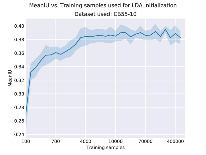
Figure 6. Stability of the LDA initialization in respect to the number of training samples used to compute it on CB55. The shaded area represents the variance whereas the tick line is the mean value, computed over 10 runs. Mind that the x-axis is not linear. Observe how as of 40k samples it seems to have reached the maximum performance.

First we evaluate the stability of the LDA initialization in respect to the number of training samples $k$ used to compute it (see Figure 6) . After validating this hyper-parameter, we will use it for all other experiments.

When initializing a multi layer network with LDA we start by computing LDA on $k$ raw input patches and use the transformation matrix to initialize the first layer. We then proceed to apply a forward pass with the first layer to all $k$ raw input patches and we use the output to compute again LDA such that we can use the new transformation matrix to initialize the second layer. This procedure is then repeated until the last layer is initialized. At this point, we add a classification layer that we will initialize in the same fashion as the others, but with the linear discriminant matrix (see Section 2) rather than with the transformation matrix. The whole procedure takes less than two minutes with our experimental setting.

Initializing with random weights

For the random initialization we trivially set the weights matrices to be randomly distributed in the range $\left[\frac{1}{-\sqrt{n}},\frac{1}{\sqrt{n}}\right]$, where $n$ is the number of inputs of the neuron of the layer being initialized.

Training phase

Once the networks are initialized (both LDA and random) we test their performance on the test set already and again after each training epoch. We then train them for $100$ epochs (where one epoch corresponds to $100K$ training samples) with mini-batches of size $4096$. We optimize using standard SGD (Stochastic Gradient Descent) with learning rate $0.01$. In order to reduce the role randomness play in the experiments, in a single run we show the same input patches to both an LDA and a random network — so that pair-wise they see the same input — and the final results are computed by averaging 10 runs.

Evaluation metric

The evaluating metric chosen is the mean Intersection over Union because is much stricter than accuracy and especially is not class-size biased (Alberti et al., 2017a). We measure it with an open-source tool.

4. Features Visualization

In this section we show and briefly discuss the features visualization of the CNN initialized with LDA. In Figure 3 are shown the features of the first three layers of the network initialized with LDA and of the first layer of a network randomly initialized, for the CSG863 manuscript.

Without surprise, the features produced by the random initialization are not visually appealing as they are very close to being just gray with noise. In fact, they are not representing something meaningful at all.

On the other hand, those produced by the LDA initialization are a completely different story. Notice how on the first layer (Figure 3a), there are 3 meaningful features, which are exactly as many as the number of classes minus one (see details in Section 2). We expected the first three features to be ”mono-color“ and much different than the others, as we know standard LDA typically projects the points in a sub-dimensional space of size $|C|-1$, where $|C|$ is the number of classes (see details in Section 2). Moreover, the other 21 features are yes, looking like the random ones, but are much more colorful. This means that their values are further away from zero.

Regarding the second and third layer (Figures 3c and 3d), as convolution is involved is difficult to interpret their visualization in an intuitive way. We can, however, observe how also in the second layer the first three features are significantly different than the other ones and how this is not entirely true anymore in the third layer.

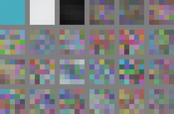
(a) First layer features (LDA) (b) First layer features (RND)

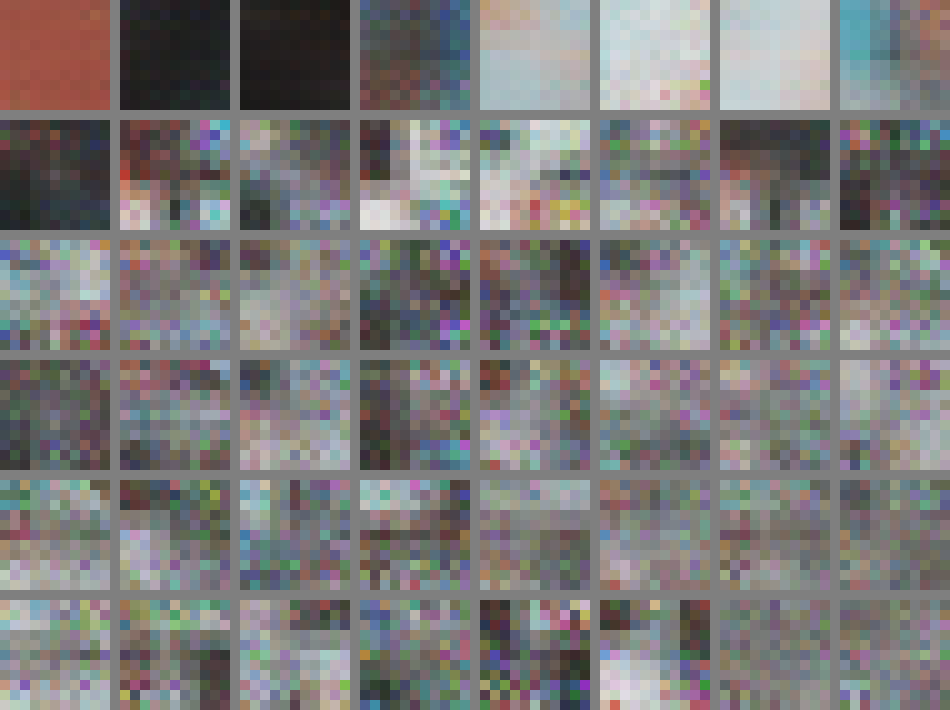
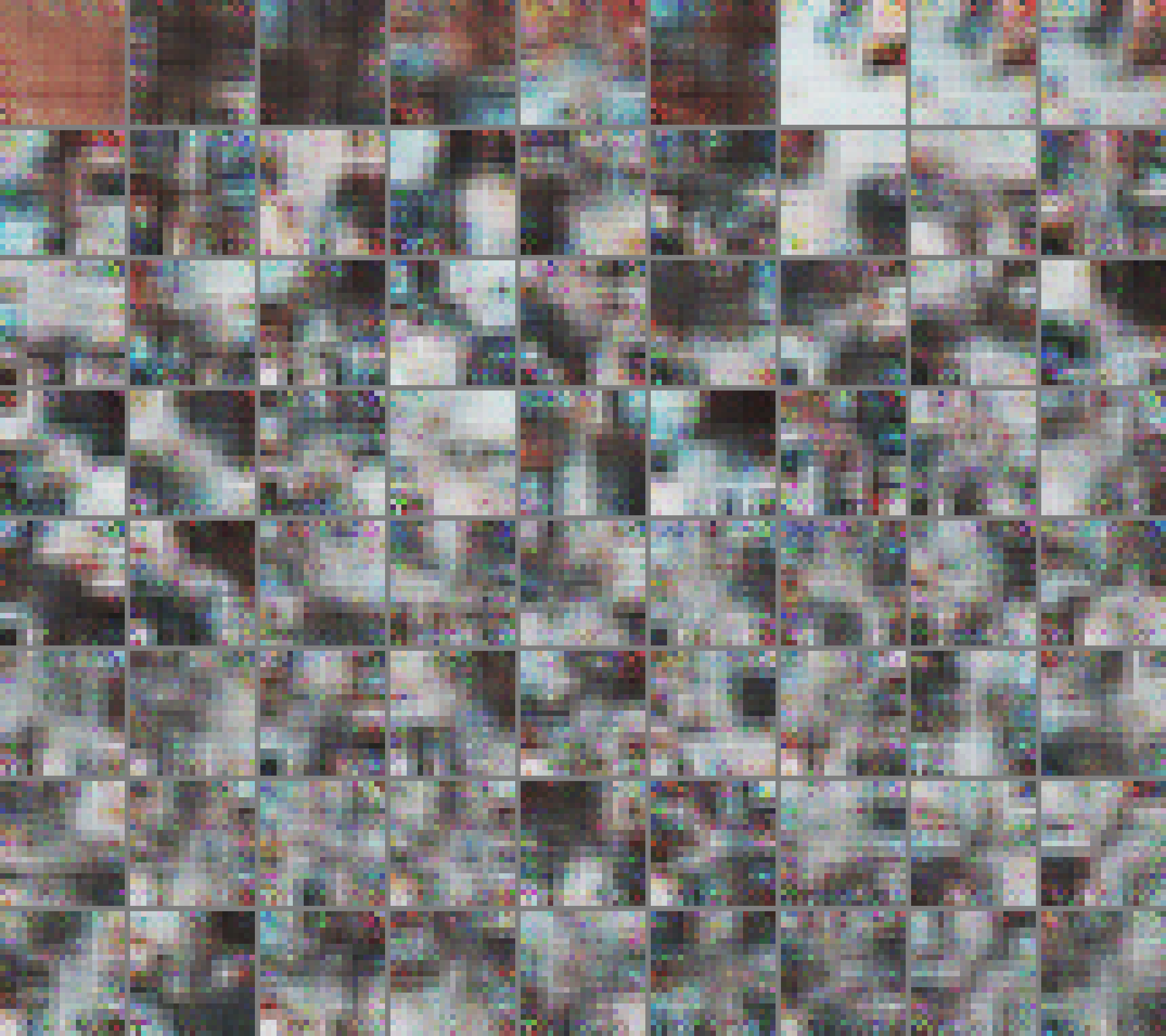
(c) Second layer features (LDA) (d) Third layer features (LDA)

Figure 3. Features of the first three layers of the network initialized with LDA and of the first layer of a network randomly initialized, for the CSG863 manuscript. Notice how the LDA ones are much more colorful than the random ones. Moreover, in (a) one can see how, as expected, there are 3 meaningful features, which are exactly as many as the number of classes minus one (see details in Sections 2 and 4).

5. Results Analysis

We measured the mean IU of networks during their training phase, evaluating them after each epoch – Figure 5 shows their performances. The LDA initialization is very stable as all networks started with almost the same mean IU. The random initialization however leads to a very high variance of the classification quality at the beginning of the training.

We can also note that the curves of the LDA-initialized networks have very similar shapes for all three manuscripts, thus their behavior can be considered as rather predictable. Contrariwise, the random initialization leads to three different curve shapes, one per manuscript, so we cannot predict how randomly-initialized networks would behave on other manuscripts.

The LDA initialization has two capital advantages over the random one. First, initial mean IU clearly outperforms randomly-initialized networks, as shown in Table 1. The table also includes the percentage of correctly classified pixels, a measurement less punitive than the mean IU but which sheds light from another angle on the advantages of LDA initialization. Second, the LDA initialization leads quickly to much better local minima. In the case of CS863, none of the 10 random networks has finished converging after 100 epochs while LDA-initialized networks have almost finished converging after 60 epochs.

These advantages can be explained by looking at the features obtained by LDA-initialization shown in Figure 3. There are useful structures for some of the filters in all three layers of the network before starting the training, thus less weight adaptations are needed.

In the case of CB55 and CS18, randomly-initialized networks seem to all find similar solutions, and end with very low mean IU variance. Observing only these results, one could think this is the best that can be obtained with the network topology we used, yet the LDA initialization proves this assertion wrong.

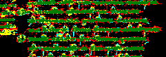
(a) LDA init network before training

(b) LDA init network after training

(c) RND init network before training

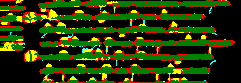
(d) RND init network after training

Figure 4. Visualization of the classification performances of both LDA and random (RND) initialized network, before and after training for a small patch of CB55. Green and black denotes correctly classified foreground and background pixels, blue and red are false negative respectively false positive foreground pixels and yellow is used for wrong foreground class e.g text instead of comment.

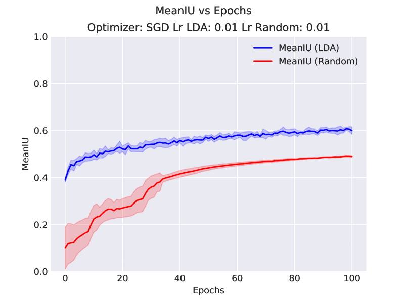
(a) Mean IU during training for CB55

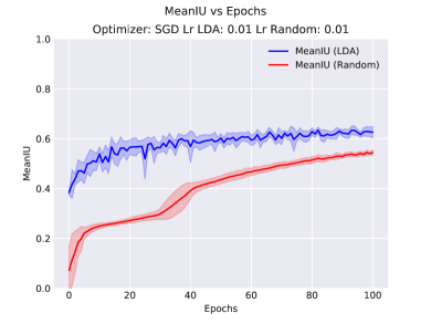
(b) Mean IU during training for CS18

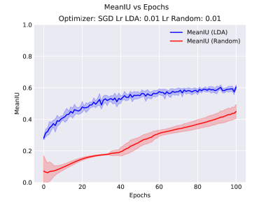
(c) Mean IU during training for CS863

Figure 5. Mean performances of the networks initialized with LDA (blue) and random weights (red) evaluated during the training. LDA networks are significantly better than the random counterpart: they start off at a very high IU and converge to a better local minima.

	Mean IU				Accuracy
model	CB55	CSG18	CSG863	AvG	AvG
LDA(init)	0.39	0.38	0.28	0.35	0.75
RND(init)	0.09	0.07	0.07	0.07	0.20
LDA(trained)	0.59	0.62	0.60	0.60	0.93
RND(trained)	0.48	0.54	0.44	0.48	0.88

Table 1. Results obtained with both LDA and random initialized networks on all manuscripts. The most-right column is the average accuracy over the whole dataset. We added it to emphasize the strictness of the Mean IU metric, which is always much lower than the accuracy, as it is not class-size biased.

6. Conclusion and Outlook

In this paper, we have investigated a new approach for initializing DNN using LDA. We show that such initialization is more stable, converge faster and to better performances than the random weights initialization. This leads to significantly shorter training time for layout analysis tasks at the cost of an initialization time that can be considered as negligible.

This study has been conducted only on relatively small CNN, so the generality of the aforementioned findings should be investigated for deeper networks. Also, as the focus was not achieving high level of accuracy, the design of our test is kept small and simple. Consequently, the results obtained should not be compared to state of art ones.

As future work, we intend to study the joint use of multiple statistical methods (such as PCA and LDA) to initialize a much deeper DNN and to extend the performances test to other classification tasks (e.g image recognition, digit recognition).

Finally, we believe that a good network initialization might be a solution to reduce the training time of DNN significantly.

References

- (1)
- Alberti et al. (2017a) Michele Alberti, Manuel Bouillon, and Rolf Ingold. 2017a. Open Evaluation Tool for Layout Analysis of Document Images. CoRR (2017).
- Alberti et al. (2017b) Michele Alberti, Mathias Seuret, Rolf Ingold, and Marcus Liwicki. 2017b. Questioning the Correlation between Reconstruction and Classification Abilities of Deeply Learned Features. CoRR (2017).
- Alberti et al. (2017c) Michele Alberti, Mathias Seuret, Rolf Ingold, and Marcus Liwicki. 2017c. What You Expect is NOT What You Get! Questioning Reconstruction/Classification Correlation of Stacked Convolutional Auto-Encoder Features. CoRR abs/1703.04332 (2017). http://arxiv.org/abs/1703.04332
- Ballard (1987) Dana H Ballard. 1987. Modular Learning in Neural Networks.. In AAAI. 279–284.
- Bottou (1988) LY Bottou. 1988. Reconnaissance de la parole par reseaux multi-couches. In Proceedings of the International Workshop Neural Networks Application, Neuro-Nimes, Vol. 88. 197–217.
- Caruana (1998) Rich Caruana. 1998. Multitask learning. In Learning to learn. Springer, 95–133.
- Demir and Ozmehmet (2005) G.K. Demir and K. Ozmehmet. 2005. Online local learning algorithms for linear discriminant analysis. Pattern Recognition Letters 26, 4 (2005), 421 – 431. https://doi.org/10.1016/j.patrec.2004.08.005 ICAPR 2003.
- Diaf et al. (2013) A. Diaf, B. Boufama, and R. Benlamri. 2013. Non-parametric Fisher’s discriminant analysis with kernels for data classification. Pattern Recognition Letters 34, 5 (2013), 552 – 558. https://doi.org/10.1016/j.patrec.2012.10.030
- Friedman et al. (2001) Jerome Friedman, Trevor Hastie, and Robert Tibshirani. 2001. The elements of statistical learning. Vol. 1. Springer series in statistics New York.
- Goodfellow et al. (2016) Ian Goodfellow, Yoshua Bengio, and Aaron Courville. 2016. Deep Learning. MIT Press. http://www.deeplearningbook.org.
- Hinton et al. (2006) Geoffrey Hinton, Simon Osindero, and Yee-Whye Teh. 2006. A Fast Learning Algorithm for Deep Belief Nets. Neural Comput. 18, 7 (jul 2006), 1527–1554. https://doi.org/10.1162/neco.2006.18.7.1527
- Kavzoglu (1999) Taskin Kavzoglu. 1999. Determining optimum structure for artificial neural networks. In Proceedings of the 25th Annual Technical Conference and Exhibition of the Remote Sensing Society. Remote Sensing Society Nottingham, UK, 675–682.
- Krähenbühl, Philipp and Doersch, Carl and Donahue, Jeff and Darrell, Trevor (2015) Krähenbühl, Philipp and Doersch, Carl and Donahue, Jeff and Darrell, Trevor. 2015. Data-dependent Initializations of Convolutional Neural Networks. arXiv preprint arXiv:1511.06856 (2015).
- Martinez and Kak (2001) A. M. Martinez and A. C. Kak. 2001. PCA versus LDA. IEEE Transactions on Pattern Analysis and Machine Intelligence 23, 2 (Feb 2001), 228–233. https://doi.org/10.1109/34.908974
- Matthias et al. (2015) Dorfer Matthias, Kelz Rainer, and Widmer Gerhard. 2015. Deep Linear Discriminant Analysis. CoRR abs/1511.04707 (2015). http://arxiv.org/abs/1511.04707
- McCulloch and Pitts (1943) Warren S McCulloch and Walter Pitts. 1943. A Logical Calculus of the Ideas Immanent in Nervous Activity. The bulletin of Math. Biophysics 5 (1943), 115–133.
- Osuna ([n. d.]) Ricardo Gutierrez Osuna. [n. d.]. L10: Linear Discriminants Analysis. Pattern Analysis, PDF online. ([n. d.]).
- Pletschacher and Antonacopoulos (2010) Stefan Pletschacher and Apostolos Antonacopoulos. 2010. The PAGE (page analysis and ground-truth elements) format framework. In Pattern Recognition (ICPR), 2010 20th International Conference on. IEEE, 257–260.
- Raschka (2014) Sebastian Raschka. 2014. Linear Discriminant Analysis – Bit by Bit. (apr 2014). http://sebastianraschka.com/Articles/2014_python_lda.html
- Schmidhuber (2015) Jürgen Schmidhuber. 2015. Deep Learning in Neural Networks: An Overview. Neural Networks 61 (2015), 85–117. https://doi.org/10.1016/j.neunet.2014.09.003 Published online 2014; based on TR arXiv:1404.7828 [cs.NE].
- Seuret et al. (2017) Mathias Seuret, Michele Alberti, Rolf Ingold, and Marcus Liwicki. 2017. PCA-Initialized Deep Neural Networks Applied To Document Image Analysis. Accepted ICDAR 2017 abs/1702.00177 (2017). http://arxiv.org/abs/1702.00177
- Simistira et al. (2017) Foteini Simistira, Mathias Seuret, Manuel Bouillon, Marcel Würsch, Michele Alberti, Marcus Liwicki, and Rolf Ingold. 2017. ICDAR2017 competitionon Layout Analysis for Challenging Medieval Manuscripts. In 2017 International Conference on Document Analysis and Recognition. to appear.
- Simistira et al. (2016) Foteini Simistira, Mathias Seuret, Nicole Eichenberger, Angelika Garz, Marcus Liwicki, and Rolf Ingold. 2016. Diva-hisdb: A precisely annotated large dataset of challenging medieval manuscripts. In Frontiers in Handwriting Recognition (ICFHR), 2016 15th International Conference on. IEEE, 471–476.
- Smolensky (1986) Paul Smolensky. 1986. Parallel Distributed Processing: Explorations in the Microstructure of Cognition. Vol. 1. MIT Press, Cambridge, USA. 194–281 pages.
- Wang et al. (1994) Changfeng Wang, Santosh S Venkatesh, and J Stephen Judd. 1994. Optimal stopping and effective machine complexity in learning. Advances in neural information processing systems (1994), 303–303.
- Wang et al. (2010) Jinghua Wang, Yong Xu, David Zhang, and Jane You. 2010. An efficient method for computing orthogonal discriminant vectors. Neurocomputing 73, 10–12 (2010), 2168 – 2176. https://doi.org/10.1016/j.neucom.2010.02.009 Subspace Learning / Selected papers from the European Symposium on Time Series Prediction.
- Webb and Lowe (1990) Andrew R Webb and David Lowe. 1990. The optimised internal representation of multilayer classifier networks performs nonlinear discriminant analysis. Neural Networks 3, 4 (1990), 367 – 375. https://doi.org/10.1016/0893-6080(90)90019-H