A Fast and Generic GPU-Based Parallel Reduction Implementation

Abstract

Reduction operations are extensively employed in many computational problems. A reduction consists of, given a finite set of numeric elements, combining into a single value all elements in that set, using for this a combiner function. A parallel reduction, in turn, is the reduction operation concurrently performed when multiple execution units are available. The current work reports an investigation on this subject and depicts a GPU-based parallel approach for it. Employing techniques like Loop Unrolling, Persistent Threads and Algebraic Expressions to avoid thread divergence, the presented approach was able to achieve a 2.8x speedup when compared to ???, using a generic, simple and easily portable code. Experiments conducted to evaluate the approach show that the strategy is able to perform efficiently in AMD and NVidia’s hardware, as well as in OpenCL and CUDA.

Walid Jradi^a∗, Hugo do Nascimento and Wellington Martins
^aUniversidade Federal de Goiás – Instituto de Informática
Alameda Palmeiras, Quadra D, Campus Samambaia
CEP 74690-900 – Goiânia – Goiás

1 Introduction

Widely used as a basic subroutine for a number of algorithms such as Counting Sort [6], Stream Compaction [2], Golden Section and Fibonacci Methods [18] and Radix Sort [6, Chapter 8.3].

The remainder of this paper is structured as follows. Section 1.1 presents some basic concepts. Section 2 briefly describes the techniques currently in use. Section 3 explains our approach. Section 4 details the experimental environment and the results. Finally, Section 5 gives general remarks about the presented strategy.

1.1 Problem Definition

Formally, a reduction can be defined as follows [24]: Given a set X with n values, $X=\{x_{0},x_{1},...,x_{n-1}\}$, compute $x_{0}\otimes x_{1}\otimes...\otimes x_{n-1}$. The associative operator $\otimes$ (also known as combiner function) can be (but is not limited to) any one of the set $\{+,\times,\wedge,\vee,\oplus,\cap,\cup,\max,\min\}$.

Consider the pseudo code shown in Algorithm 1. At first glance, it seems that the algorithm is inherently sequential, since the variable accumulator depends on the value computed in the previous step, preventing any attempt of parallelization. However, it is possible to avoid this problem by making use of two basic properties of addition and multiplication operations: Associativity and Commutativity.

Input: A set $A=\{a_{1},a_{2},\ldots,a_{n}\}$ of numeric elements

Output: The sum of all elements

1

2$accumulator\leftarrow 0$

3 for $i\leftarrow 1$ to $n$ do

4       $accumulator\leftarrow accumulator+a_{i}$

5      

6return $accumulator$

Algorithm 1 Summation(A)

• Associativity means that, given three or more numbers, they can be linked in any order without changing the final result. Taking the sum as an example, it’s possible to do $a_{1}+a_{2}$ and, then, add $a_{3}$, and the result will be the same as doing $a_{3}+a_{2}$ and then adding $a_{1}$. Formally, we have $(a_{1}+a_{2})+a_{3}\equiv a_{1}+(a_{2}+a_{3})$;

• Commutativity ensures that no matter the order in which an operation on two numbers $a_{1}$ and $a_{2}$ is performed, the result will always be the same. Formally, for multiplication, we have $a_{1}\cdot a_{2}\equiv a_{2}\cdot a_{1}$.

Considering that the order in which the elements are combined does not affect the final result^, , these two properties can be used, dividing the problem into smaller subproblems and these, in turn, solved in parallel. After solving each subproblem, the partial results are combined to produce the final result. Figure 1 illustrates the process using the associative operator “$+$” in an array with 16 elements.

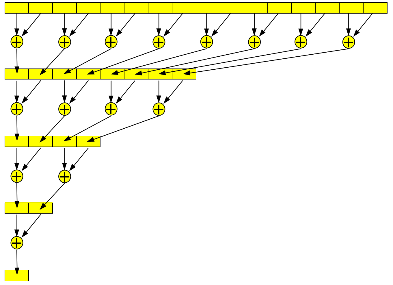
Figure 1: Parallel reduction – associative reduction tree.

2 Parallel Reduction in GPUs

Since the arrival of programmable GPUs, some strategies to accelerate the reduction operation on such devices have been proposed. The two most well known are those described by Mark Harris [14] and Bryan Catanzaro [3]. Most recently, Justin Luitjens [19] presented some improvements to the strategies described in [14]. Unfortunately, the strategies adopted by [14] and [19], although very efficient, are limited to hardware and software provided by NVidia, restricting their use.

On the other hand, the proposal of Catanzaro [3] is based on the open standard OpenCL [11], adopted by a myriad of manufacturers, what makes it portable. Nevertheless, the code presented in [3] also has a weakeness, as it does not adopt some strategies that could significantly improve its performance.

This section details how the associative and commutative properties can be used to implement efficient parallel reductions on GPUs. As highlighted at the end of Section 1.1, the basic idea is to “split” the problem into smaller pieces and solve them in parallel. However, the execution environment (GPU hardware) imposes some restrictions that must be considered to maximize the speedup. Therefore, the details of how GPUs are organized [5, 27] will dictate the choices from now on.

The approaches of Harris [14] and Catanzaro [3] to deal with reductions in GPUs operate in a pretty similar way, using a tree-based structure.

One of the aspects to be considered is the number of elements in the collection (vector) in which the reduction will be applied. If this amount is sufficiently small and can be stored in the local memory of each SM, then the reduction becomes quite simple. In [3], Catanzaro presents some strategies for this case and conducts performance comparisons between them. Then, after describing how reductions can be efficiently performed in small sets, Catanzaro shifts his focus to the cases in which a large volume of data must be handled. Three strategies are presented and a winner, called “Two-Stage Parallel Reduction”, is elected. Harris [14] deals only with parallel reduction in large datasets.

Our approach is mainly based on a proposal from Catanzaro [3]. Therefore, a more detailed description of it is presented. First, however, we also give an explanation of the strategies by Harris [14] and Luitjens [19], since some ideas for speeding up the computation came from them. Hence, unlike the rest of the thesis, here their original code is presented, and not just the pseudo code.

2.1 Mark Harris’ Work

The work presented by Harris [14] focuses on techniques for performing reductions of large data volumes. The author shows, through successive versions of the same algorithm, how bad decisions or an incorrect way of mapping the problem to the target platform can negatively impact the application performance.

Problems like shared memory bank conflict, lack of communication between thread blocks (making it impossible for a kernel to reduce a large array at once) and highly divergent warps are addressed. Starting with a naive version, step by step improvements are described, reaching an implementation 30x faster than the first one. Next, we show how the author achieved such speedups.

Harris performed experiments using a G80 GPU. This video card has a 384-bit memory interface, with a 900 MHz DDR memory, which leads to a theoretic $\frac{384\ast 1800}{8}=86.4GB/s$ of memory bandwidth. All tests were conducted using a vector with $2^{22}$ (4M) integer values.

As a result of all the applied optimizations, the final version of the code runs in 0.268ms and the memory bandwidth usage reaches 62.671GB/s. All these improvements are summarized in Table 1.

	Time (ms)	Memory Bandwidth (GB/s)	Step speedup	Cummulative speedup
Kernel 1: interleaved addressing with divergent branching	8.054	2.083
Kernel 2: interleaved addressing with bank conflicts	3.456	4.854	2.33x	2.33x
Kernel 3: sequential addressing	1.722	9.741	2.01x	4.68x
Kernel 4: first add during global load	0.965	17.377	1.78x	8.34x
Kernel 5: unroll last warp	0.536	31.289	1.8x	15.01x
Kernel 6: completely unrolled	0.381	43.996	1.41x	21.16x
Kernel 7: multiple elements per thread	0.268	62.671	1.42x	30.04x

Table 1: Performance for parallel reduction of $2^{22}$ integer elements (extracted from [14]).

2.2 Justin Luitjens’ Work

In [19] Luitjens shows how a new feature of the NVidia’s Kepler (and newer) GPU architecture can be used to make reductions even faster when compared to the strategies presented in [14]: the shuffle (SHFL) instruction.

Usually, work-items inside the same SM use the local (shared) memory when they need to communicate (exchange information). This involves a three-step process: writing the data to local memory, perform a synchronization barrier and then read the data back from local memory. The Kepler and newer architectures implement the shuffle instruction, which enables a work-item to directly read private data from another work-item in the same wave-front. According to the author, there are four main advantages in using this instruction:

• It ultimately allows work-items inside a wave-front to collectively exchange or broadcast data;

• It replaces the three-step process by a single instruction, effectively increasing the bandwidth and decreasing the latency;

• It does not use the local memory at all;

• A sync barrier is implicit in the instruction and, hence, a synchronization step inside a workgroup is not necessary.

Figure 2 shows how this instruction can be used to build a reduction tree. As pointed out by Luitjens, this figure only includes the arrows for the work-items actually doing useful work. All work-items are indeed shifting values even though these values are not necessary in the reduction process.

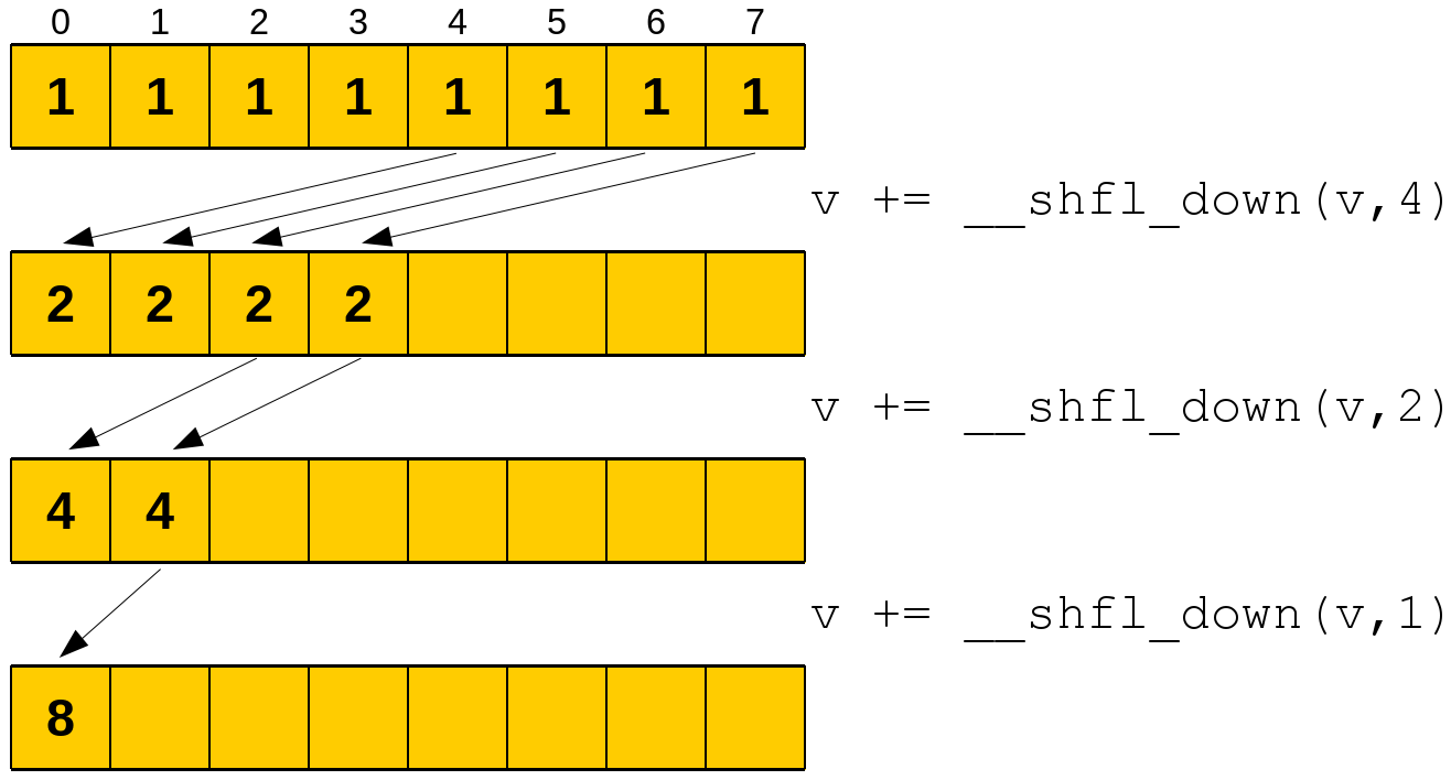
Figure 2: Parallel reduction using the shuffle instruction (extracted from [19]).

Using this instruction, several versions of the reduction were proposed, implemented and compared. However, although Luitjens states that the adopted strategies lead to faster reductions than those described by Harris [14], no comparative studies between the two approaches were conducted.

2.3 Bryan Catanzaro’s Work

Now, we describe Catanzaro’s two-stage parallel reduction approach for large datasets, as presented in [3].

The technique is based on dividing the data set in p pieces (or “chunks”), where p is large enough to keep all GPU cores busy. It is also necessary to limit the number of work-items to the maximum amount that the GPU can handle in total without having to switch between them (from now on, that maximum will be called GS – or global size). Each chunk is then processed by a work-group.

Since the sum operation has the properties of associativity and commutativity, each work-item can perform its own reduction sequentially and intercalary with the others. A work-item takes, as the starting point, its global identifier and accumulates, in a private variable, its partial sum, skipping GS positions at every step in the vector stored in the GPU’s global memory.

After having completed a pass through the data set, the work-items in each workgroup write the result of their own reduction in a scrap vector located in local/shared memory which, in turn, will also be reduced in parallel. At the end of the process, each working group will have its own scrap containing, in its position 0, the result of the reduction so far. This partial result is then copied to another vector, this time stored in the GPU global memory, which size must be equal to —SM—. The first stage is then complete. Its source code, extracted from [3], is presented in Listing 1.

Listing 1: Two-stage parallel reduction of Catanzaro – stage 1

⬇

__kernel void reduce(__global float* buffer,

__local float* scratch,

__const int length,

__global float* result) {

int global_index = get_global_id(0);

float accumulator = INFINITY;

// Loop sequentially over chunks of input vector

while (global_index < length) {

float element = buffer[global_index];

accumulator = (accumulator < element) ? accumulator : element;

global_index += get_global_size(0);

}

int local_index = get_local_id(0);

scratch[local_index] = accumulator;

barrier(CLK_LOCAL_MEM_FENCE);

// Perform parallel reduction

for(int offset=get_local_size(0)/2; offset>0; offset=offset/2) {

if (local_index < offset) {

float other = scratch[local_index + offset];

float mine = scratch[local_index];

scratch[local_index] = (mine < other) ? mine : other;

}

barrier(CLK_LOCAL_MEM_FENCE);

}

if (local_index == 0) {

result[get_group_id(0)] = scratch[0];

}

}

The second stage is simpler. Since now there is a vector with $|SM|$ elements in the global memory – with the result of a partial sum in each position – just the first $|SM|$ work-items of the first $SM$ copy their corresponding value to an array allocated in local memory. Then the work-items perform a new parallel sum of the elements in the vector. After copying the value in position 0 back to global memory, the reduction is finally complete.

The next sections detail some advanced techniques to further explore parallelism and that were extensively used in the present work.

2.4 Loop Unrolling

Loop Unrolling (also known as Loop Unwinding and Loop Unfolding) is an optimization technique – performed by the compiler or manually by the programmer – applicable to certain kinds of loops in order to reduce (or even prevent) the occurrence of execution branches and minimize the cost of instructions for controlling the loop [1, 8, 16, 25]. Its goal is to optimize the program’s execution speed at the expense of increasing the size of the generated code (space-time tradeoff). It is easily applicable to loops where the number of executions is previously known, like routines of vector manipulation where the number of elements is fixed.

Basically the technique consists in the reuse of the sequence of instructions being executed within the loop, so as to include more of an iteration of the code every time the loop is repeated, reducing the amount of these repetitions.

This reuse is done by manually replicating the code inside the loop a certain amount of times or through the “#pragma unroll n” positioned immediately before the beginning of the loop. The number of times the loop is unrolled is called Unrolling Factor and, with the pragma directive, it is given by the parameter “n”.

It is worth noting that with the pragma directive we leave the decisions of how the loop should be unrolled to the compiler, which may lead to a not so optimized resulting code. In the experiments performed as part of this work, the best results were always achieved using manual loop unrolling.

As an example, consider the C code shown in Listing 2, which simply multiplies the elements of an array by its index ($a_{i}\leftarrow a_{i}\cdot i$). In this example, we call L the loop size and F its unrolling factor. L here is equal to 100.

Listing 2: Multiplying elements in a vector

⬇

for (int i = 0; i < 100; i++) {

a[i] = a[i] * i;

}

It’s possible to significantly improve the execution speed of this algorithm by unrolling it, as shown in Listing 3.

Listing 3: Unrolling the multiply routine

⬇

for (int i = 0; i < 100; i += 3) {

a[i] = a[i]*i;

a[i+1] = a[i+1]*(i+1);

a[i+2] = a[i+2]*(i+2);

}

The two extra lines of code and the “i += 3” in Listing 3 performs the desired three-fold ($F=3$) manual loop unrolling.

As it can be seen, the $\frac{L}{F}$ ratio does not necessarily need to be an integer. If it admits a remainder, the compiler can (since the number of iterations is previously known at compile time) add extra code to the end of the unrolled generated code in order to ensure its correctness.

Unrolling, when applicable, offers several advantages over non-unrolled code. Besides the decrease in the number of iterations, an increase occurs in the amount of work done each time through the loop. This also open ways for the exploration of parallelism by the compiler in machines with multiple execution units, since each instruction within the loop can be handled by an independent thread.

However, these are only the most easily perceivable benefits. Agner Fog [8] listed several others, as well as some observations about when this technique should be avoided. Such factors (advantages and disadvantages) must be considered by the programmer when deciding to use loop unrolling or not.

2.5 Persistent Threads

Since the launch of the first programmable GPUs and with all its basic architecture inspired by the SIMD model, the “Single Instruction Multiple Thread” (SIMT) and “Single Program Multiple Data” (SPMD) paradigms have become standards de facto. Both seek to hide the details of the underlying hardware where the code runs, attempting to facilitate the painful task of development [12].

Gupta et al. [12] argue that the usage of these “traditional” paradigms greatly limits the actions of the programmer, because all control of the execution flow is in the power of the scheduler’s video card. This programming style, which delegates all the decisions to the scheduler, is called by the authors as “non-PT”, or “non-Persistent”.

It requires that the software developer abstracts units of work to virtual work-items. Since the number of wave-fronts to create is based on the number of virtual work-items, during a kernel launch usually there are several hundreds of even thousands more wave-fronts to be executed than the amount of physical processing elements to assign them to.

Such scheduling of wave-fronts is performed by the scheduler and the programmer has no means to interfere in the process, e.g., how, where, when and in which order the work-groups will be assigned.

Gupta et al. claim that, while these abstractions reduce the effort for new developers in the GPGPU field, they also create obstacles for experienced programmers, who normally face problems for which workload is inherently irregular, therefore making it much more difficult to efficiently parallelize when compared to problems whose parallel solution is more regular.

According to Gupta et al., this uncovers a serious drawback of the current SPMD programming style, which is not able to ensure order, location and timing. It also does not allow the software developer to regulate these three parameters without completely avoiding the GPU scheduler.

Thus, to overcome these limitations, developers have been using a programming style called Persistent Threads (“PT”), whose low level of abstraction allows performance gains by directly controlling the scheduling of work-groups. And although this style has been in use for some time, only in 2012 it was formally introduced, described and analyzed by Gupta et al. [12]. They also list several problems when adopting the traditional style.

Basically, what the PT style change is the lifetime of a work-item [23], by letting it keep running longer and giving it much more work than in the traditional “non-PT” style [26]. This is done circumscribing the logic kernel (or part of it) in a loop, so this loop remains running while there are items to be processed.

Briefly, from the point of view of the developer, all work-items are active while the kernel is running. As a direct consequence of PT, a kernel should be triggered using only the amount of work-items that can be executed concurrently by each Streaming Multiprocessor. All these actions will prevent constant return of control to the host and the cost of new kernel invocations [23].

Gupta et al. acknowledge, however, that the technique of Persistent Threads is not a panacea, and its use should be carefully evaluated [12]. In particular, the technique fits well when the amount of memory accesses is limited (i.e., few reading/writing to global memory and a large volume of computation) and the problem being solved has not many initial input elements or the growth in the number of elements in the input set is fairly limited. Beyond these conditions, the traditional non-PT style tends to outperform the PT style.

2.6 Thread Divergence

Current GPUs are able to deliver massive computational power at a reasonably low cost. However, due to the way they are constructed, some obstacles must be overcome for the effective use of such power. One of the main and hardest obstacles to avoid is the presence of conditional statements [28] potentially leading to branches in the execution flow of the various work-items [13].

By default, GPUs try to run all the work-items inside the wave-fronts in the SIMD model. However, if the code being executed has conditional statements that lead to divergences in program flow, the divergent work-items will be stalled and its execution will only happen after the non-stalled work-items have completed their runs, which ultimately compromises the desired speedup. This phenomenon is called Thread Divergence [4, 13, 22, 28].

Trying to circumvent this problem, some strategies have been proposed in order to minimize or even eliminate the effects of such phenomena. Among them, we cite [4, 9, 13, 20, 22, 28].

—:::

Wherefore it became necessary to develop a method to prevent flow divergence, which could ultimately compromise the performance of such a step of computation. The method is detailed at the end of Section 3.

3 The New Approach

The improvements proposed in our work focus on Steps 1 and 3 of the first stage of the reduction presented in Section 2.3. The improvements employ the same strategies proposed by Harris [14] to increase the performance of the approach originally presented by Catanzaro [3] but with appropriately chosen interventions.

In step 1 of the original implementation, the vector in global memory containing the data to be reduced is entirely traversed by the work-items, each one performing its own reduction.

This step already uses the “Persistent-Thread” strategy, but its performance can be improved by adopting loop unrolling (Section 2.4). As it can be seen, instead of doing the unroll when the data is in local memory, as proposed by Harris [14] (Listings LABEL:code:ParallelReductionMH5 and LABEL:code:ParallelReductionMH6 of Section 2.1), our improvement performs the unroll in the global memory.

The code presented in Listing 4 shows the modified loop, assuming an unrolling factor (F) equals to 4, $iGlobalID$ as the work-item global identifier and $iLength$ as the number of elements to be reduced.

Listing 4: Unrolling the step 1

⬇

for (iPos = iGlobalID*iUnrollingFactor; iPos < iLength;

iPos += iGlobalSize*iUnrollingFactor)

{

i0 = iPos; i1 = iPos+1; i2 = iPos+2; i3 = iPos+3;

accumulator +=

((i0<iLength)*(aVector[i0])+

(i1<iLength)*(aVector[i1])+

(i2<iLength)*(aVector[i2])+

(i3<iLength)*(aVector[i3]));

}

A special attention must be given to how the data is brought from the global memory (aVector) to the private memory (accumulator), through the use of algebraic expressions that prevent reading from invalid memory locations, thus avoiding the usage of “ifs” and potential divergences in the execution flow. The expression $i_{n}<iLength$ expands to integers 1 or 0 whether it is, respectively, true or false. In the first case ($i_{n}<iLength)*(aVector[i_{n}])$ is interpreted as $(1)*(aVector[i_{n}])$, adding the value stored in location $i_{n}$ to the partial sum (accumulator). In the second case, the expression is interpreted as $(0)*(aVector[0])$, ensuring that – regardless of the data stored in the first position of the vector – value 0 is added to accumulator, keeping the partial sum correctness.

At the begining of Step 3, the resulting values of the previous sums are already stored in the local memory of the SMs. Then, each SM performs its own local reduction with its work-items.

In the solutions presented by Harris [14] and Catanzaro [3], in this step all work-items are kept synchronized through the use of barriers. However, with minor conceptual changes, it is possible to completely eliminate the overhead caused by the barriers, not only in the last 6 iterations of the loop, as proposed by Harris [14].

Our strategy is to use algebraic expressions to keep all the work-items in the same execution step, maintaining its desired behaviour and algorithm correctness.

Consider the highly divergent code presented in Listing LABEL:code:ThreadDivergence2 (Section 2.6). Using a simple algebraic expression, it can be rewriten in order to completely eliminate the conditional statement and still return the right result of the comparison, as can be seen in Listing 5.

Listing 5: Algebraic “if-then-else”

⬇

int smallestValue(int a, int b) {

return (a < b) * a + (a >= b) * b;

}

Note that the two boolean operations ($(a<b)$ and $(a>=b)$) are mutually exclusive, being interpreted internally by the compiler as 0 (false) or 1 (true). So, assuming that a is smaller than b, the result of the algebraic operation is (1) * a + (0) * b which, ultimately, will return only the value of a.

The same strategy can be applied to lines 1 to 1 of Listing 1, that represent the third step of the first stage. The new code is shown in Listing 6, where $iLocalSize$ stores the number of active local work-items and $iLI$ represents the work-item’s local identifier.

Listing 6: Avoiding Divergences

⬇

for (iPos = iLocalSize/2; iPos > 0; iPos >>= 1)

{

bFlag = iLI < iPos;

scratch[iLI] += (bFlag)*(scratch[iLI + (bFlag)*iPos]);

}

Here, in each iteration of the loop, $iPos$ is divided by 2 (iPos ¿ ¿ = 1) and $bFlag$ is expanded to either 1 or 0, thus reducing by half the number of work-items doing a useful job. If, for the current work-item, the expression $iLI<iPos$ becomes true, then the expression in the last line will be interpreted as $scratch[iLI]+=(1)*(scratch[iLI+(1)*iPos])$, ensuring that the value stored in position $iLI+iPos$ will be added to the value in position $iLI$. On the other hand, if the expression becomes false, it will be interpreted as $scratch[iLI]+=(0)*(scratch[iLI+(0)*iPos])$, ensuring that the value in position $iLI$ will not be considered. Since all work-items are always in the same step of computation – doing exactly the same job (useful or not), independently of being in the same wavefront – sync barriers are unnecessary.

4 Computational Experiments

Table 2 and Figures 3 and 4 represent the performance gains achieved against the algorithm described in [3], where $F=1$ is the runtime of the original code. The machine used in the tests was the same one presented in Section LABEL:sec:cc_results_gpu.

All tests were run on two vectors, one of integers and one of single precision floating points, containing 5533214 elements. There were no measurable differences between the two vector types.

The times listed in Table 2 were obtained with the OpenCL profiler CodeXL, version 2.0.12400.0, and are the averages of five consecutive executions for each F.

As can be seen, these results show that the version of the algorithm with $F=8$ reached a speedup pretty close to 2.8x, when compared with the proposal of [3]. It may also be noted that such speedup stabilizes around this value ($F=16$ provided just over 1.5% gain when compared to $F=8$).

F	Time (ms)	Speedup	Memory Bandwidth (GB/s)	Bandwidth Usage (%)
1	0.249780	1	88.6094002722	26.63
2	0.173930	1.4360949807	127.2515149773	38.24
3	0.139260	1.7936234382	158.9318971708	47.76
4	0.127700	1.955990603	173.3191542678	52.08
5	0.113930	2.1923988414	194.2671464935	58.37
6	0.100810	2.4777303839	219.5502033528	65.97
7	0.093740	2.6646042245	236.1089822914	70.95
8	0.089490	2.7911498491	247.3221142027	74.32
16	0.088160	2.8332577132	251.0532667877	75.44

Table 2: Parallel reduction execution times. New approach compared against Catanzaro’s original code.

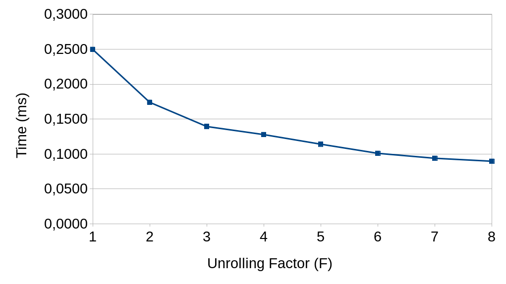
Figure 3: Chart of the parallel reduction execution times.

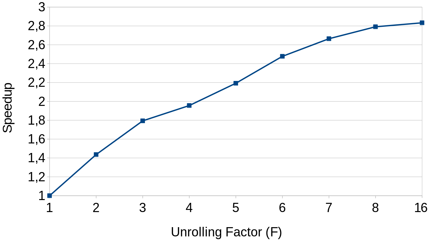
Figure 4: Chart of the parallel reduction speedup.

The same code was implemented in CUDA and tests were performed against the Kernel 7 of Harris presented in Section 2.1. The GPU used in the experiments was a Tesla C2075 with 6GB of memory. The architecture of such a video card provides 448 CUDA cores, a GPU clock of 575MHz and a shader clock of 1150Mhz. Its memory is clocked at 750MHz (3.0GHz effective).

The experiments employed the same two vectors containing 5533214 elements (integers and single precision floating points). Several values of the unrolling factor ($F$) were used in order to find the optimal value for such a video board. It was determined that up to $F=6$ the performance gains were substantial and, with $F\geq 8$, the gains were very discrete. According to this, all experiments were conducted using $F=8$. Table 3 presents the running time (in milliseconds) of both approaches and the percentage of performance (given by the formula $\frac{100\ast T_{new}}{T_{k7}}$).

Time – Kernel 7	Time – New Approach	% of Performance
0.17766 ms	0.17867 ms	99.4

Table 3: Parallel reduction execution times – new approach (with unrolling factor equals to 8) compared against Harris’ code.

5 General Remarks

Reduction operations are widely employed in many computational problems. This chapter showed how such operations can be performed in a parallel fashion using graphics processing units and detailed the main approaches for them nowadays.

All parallel reduction techniques currently in use suffer from some basic issues. Several only reach their peak performance by employing proprietary strategies and/or technologies, what ends up limiting their use to the platform for which they were designed. Others, though generic, do not adopt certain procedures that could increase their performance without loss of generality.

The strategy presented here combines the best of both worlds: It is generic enough to be used with both CUDA and OpenCL and can run on hardware of the two major GPU manufacturers with minimal changes, just being adapted to the particularities of each platform. The implemented code, besides simpler, offered a performance equivalent to the best strategy described by Harris [14].

A good performance of this routine is essential for the efficient execution of the macroscopic urban traffic assignment algorithm described in Chapter LABEL:chapter:traffic_assignment_problem, since it is used on two occasions: in the computation of shortest paths and in the golden ratio method.

References

- [1] M. Abrash. Michael Abrash’s Graphics Programming Black Book, Special Edition, The Coriolis Group. Inc., Arizona, 1997.
- [2] M. Billeter, O. Olsson, and U. Assarsson. Efficient Stream Compaction on Wide SIMD Many-Core Architectures. In Proceedings of the Conference on High Performance Graphics 2009, HPG ’09, pages 159–166, New York, NY, USA, 2009. ACM.
- [3] B. Catanzaro. OpenCL Optimization Case Study: Simple Reductions. http://developer.amd.com/resources/documentation-articles/articles-whitepapers/opencl-optimization-case-study-simple-reductions/, Aug. 2010. published by Advanced Micro Devices. Last accessed in January 05, 2014.
- [4] I. Chakroun, M. Mezmaz, N. Melab, and A. Bendjoudi. Reducing Thread Divergence in a GPU-Accelerated Branch-and-Bound Algorithm. Concurrency and Computation: Practice and Experience, 25(8):1121–1136, 2013.
- [5] S. Che, M. Boyer, J. Meng, D. Tarjan, J. W. Sheaffer, and K. Skadron. A Performance Study of General-Purpose Applications on Graphics Processors Using CUDA. Journal of Parallel and Distributed Computing, 68(10):1370–1380, 2008. General-Purpose Processing using Graphics Processing Units.
- [6] T. H. Cormen, C. E. Leiserson, R. L. Rivest, and C. Stein. Algoritmos: Teoria e Prática. Editora Campus, 2 edition, 2002.
- [7] D. Defour and S. Collange. Reproducible floating-point atomic addition in data-parallel environment. In Computer Science and Information Systems (FedCSIS), 2015 Federated Conference on, pages 721–728, Sept 2015.
- [8] A. Fog. Optimizing Subroutines in Assembly Language: An Optimization Guide for x86 Platforms. Technical University of Denmark, 2013.
- [9] W. W. L. Fung, I. Sham, G. Yuan, and T. Aamodt. Dynamic warp formation and scheduling for efficient GPU control flow. In Microarchitecture, 2007. MICRO 2007. 40th Annual IEEE/ACM International Symposium on, pages 407–420, Dec 2007.
- [10] D. Goldberg. What every computer scientist should know about floating-point arithmetic. ACM Comput. Surv., 23(1):5–48, Mar. 1991.
- [11] K. O. W. Group et al. The OpenCL specification. version, 1(29):8, 2008.
- [12] K. Gupta, J. A. Stuart, and J. D. Owens. A Study of Persistent Threads Style GPU Programming for GPGPU Workloads. In Innovative Parallel Computing (InPar), 2012, pages 1–14. IEEE, 2012.
- [13] T. D. Han and T. S. Abdelrahman. Reducing branch divergence in GPU programs. In Proceedings of the Fourth Workshop on General Purpose Processing on Graphics Processing Units, GPGPU-4, pages 3:1–3:8, New York, NY, USA, 2011. ACM.
- [14] M. Harris and Others. Optimizing Parallel Reduction in CUDA. NVIDIA Developer Technology, 2, 2007.
- [15] N. Higham. Accuracy and Stability of Numerical Algorithms: Second Edition. Society for Industrial and Applied Mathematics, 2002.
- [16] J. C. Huang and T. Leng. Generalized Loop-Unrolling: a Method for Program Speed-Up. In in Proc. IEEE Symp. on Application-Specific Systems and Software Engineering and Technology, pages 244–248, 1997.
- [17] W. Kahan. Pracniques: Further remarks on reducing truncation errors. Commun. ACM, 8(1):40–, Jan. 1965.
- [18] J. C. Kiefer. Sequential Minimax Search for a Maximum. Proc. Am. Math. Soc., 4:502–506, 1953.
- [19] J. Luitjens. Faster Parallel Reductions on Kepler. White Paper, Feb. 2014. published by NVidia Inc. Last accessed in July 25, 2014.
- [20] J. Meng, D. Tarjan, and K. Skadron. Dynamic Warp Subdivision for Integrated Branch and Memory Divergence Tolerance. SIGARCH Comput. Archit. News, 38(3):235–246, June 2010.
- [21] J. Muller, N. Brisebarre, F. de Dinechin, C. Jeannerod, V. Lefèvre, G. Melquiond, N. Revol, D. Stehlé, and S. Torres. Handbook of Floating-Point Arithmetic. Birkhäuser Boston, 2009.
- [22] V. Narasiman, M. Shebanow, C. J. Lee, R. Miftakhutdinov, O. Mutlu, and Y. N. Patt. Improving GPU Performance via Large Warps and Two-level Warp Scheduling. In Proceedings of the 44th Annual IEEE/ACM International Symposium on Microarchitecture, MICRO-44, pages 308–317, New York, NY, USA, 2011. ACM.
- [23] R. Nasre, M. Burtscher, and K. Pingali. Data-driven versus topology-driven irregular computations on GPUs. In Parallel Distributed Processing (IPDPS), 2013 IEEE 27th International Symposium on, pages 463–474, 2013.
- [24] B. Parhami. Introduction to Parallel Processing: Algorithms and Architectures. Plenum series in computer science. Plenum Press, 1999.
- [25] V. Sarkar. Optimized Unrolling of Nested Loops. Int. J. Parallel Program., 29(5):545–581, Oct. 2001.
- [26] M. Steinberger, B. Kainz, B. Kerbl, S. Hauswiesner, M. Kenzel, and D. Schmalstieg. Softshell: Dynamic scheduling on GPUs. ACM Trans. Graph., 31(6):161:1–161:11, Nov. 2012.
- [27] N. Wilt. The CUDA Handbook: A Comprehensive Guide to GPU Programming. Pearson Education, 2013.
- [28] E. Z. Zhang, Y. Jiang, Z. Guo, and X. Shen. Streamlining GPU Applications on the Fly: Thread Divergence Elimination Through Runtime Thread-data Remapping. In Proceedings of the 24th ACM International Conference on Supercomputing, ICS ’10, pages 115–126, New York, NY, USA, 2010. ACM.