IPMU17-0143

CALT-TH-2017-059

On the Large $R$-charge Expansion

in

${\cal N}=2$ Superconformal Field Theories

Simeon Hellerman and Shunsuke Maeda

Kavli Institute for the Physics and Mathematics of the Universe (WPI)
The University of Tokyo
Kashiwa, Chiba 277-8582, Japan

Abstract

In this note we study two point functions of Coulomb branch chiral ring elements with large $R$-charge, in quantum field theories with ${\cal N}=2$ superconformal symmetry in four spacetime dimensions. Focusing on the case of one-dimensional Coulomb branch, we use the effective-field-theoretic methods of [1], to estimate the two-point correlation function ${\cal Y}_{n}\equiv|x-y|^{2n\Delta_{\cal O}}\,\left<({\cal O}(x))^{n}\,(\bar{{\cal O}}(y))^{n}\right>$ in the limit where the operator insertion ${\cal O}^{n}$ has large total $R$-charge ${{\color[rgb]{.54,.17,.888}{{\cal J}}}}=n\Delta_{\cal O}$. We show that ${\cal Y}_{n}$ has a nontrivial but universal asymptotic expansion at large ${{\color[rgb]{.54,.17,.888}{{\cal J}}}}$, of the form

$$\begin{split}{\cal Y}_{n}={{\color[rgb]{.54,.17,.888}{{\cal J}}}}!\,\left({{|{\bf N}_{\cal O}|}\over{2\pi}}\right)^{2{{\color[rgb]{.54,.17,.888}{{\cal J}}}}}\,{{\color[rgb]{.54,.17,.888}{{\cal J}}}}^{\alpha}\,\tilde{{\cal Y}}_{n}\ ,\end{split}$$

where $\tilde{{\cal Y}}_{n}$ approaches a constant as $n\to\infty$, and ${\bf N}_{\cal O}$ is an $n$-independent constant describing on the normalization of the operator relative to the effective Abelian gauge coupling. The exponent $\alpha$ is a positive number proportional to the difference between the $a$-anomaly coefficient of the underlying CFT and that of the effective theory of the Coulomb branch. For Lagrangian SCFT, we check our predictions for the logarithm ${\cal B}_{n}=\log({\cal Y}_{n})$, up to and including order $\log({{\color[rgb]{.54,.17,.888}{{\cal J}}}})$ against exact results from supersymmetric localization[2, 3, 4, 5]. In the case of ${\cal N}=4$ we find precise agreement and in the case ${\cal N}=2$ we find reasonably good numerical agreement at ${{\color[rgb]{.54,.17,.888}{{\cal J}}}}\simeq 60$ using the no-instanton approximation to the $S^{4}$ partition function. We also give predictions for the growth of two-point functions in all rank-one SCFT in the classification of [6, 7, 8, 9]. In this way, we show the large-$R$-charge expansion serves as a bridge from the world of unbroken superconformal symmetry, OPE data, and bootstraps, to the world of the low-energy dynamics of the moduli space of vacua.

1 Introduction

Recently there has been development of the properties of conformal field theories (CFTs) with global charges, in states of large quantum number [10, 11, 12, 13, 14, 1, 15, 16, 17, 18, 19, 20, 21, 22, 23, 24, 25, 26, 27, 28, 29, 30, 31, 32]. Many large quantum number analyses have studied the asymptotic expansion of operator dimensions at large quantum number $J$ (either an internal symmetry such as spin, or an internal global symmetry such as a $U(n)$ or $O(n)$ symmetry), in negative powers of the total charge $J$. In many cases these relations have been checked and remarkable agreement has been found among various methods to study such regimes: conformal bootstrap, S-matrix bootstrap, Monte Carlo simulation, and the use of effective field theory. Also, in [12] three-point functions were studied and a similar expansion was derived for OPE coefficients (equivalently, three-point functions) where at least one of the operators has large global charge $J$ (and therefore, automatically, at least two of the operators).

The general pattern emerging from these works is that the behavior of operator dimensions and OPE coefficients becomes simple in the limit of some large quantum number $J$ even in a strongly coupled system. This pattern is interesting because its robustness appears to transcend the explanations for it in the analysis of any individual case. In some cases, such as large spin in a single plane in a CFT, the explanation lies in the conformal bootstrap and looks particularly intuitive in an AdS holographic dual. For systems with large global charge carried by bosonic fields, the most readily apparent explanations appear to involve a large-charge effective field theory, in which the large-$J$ operator is well-approximated by a smooth classical solution in radial quantization. These large-quantum-number limits themselves appear to be special cases of an even more general situation, a "macroscopic limit" in which one takes pure or mixed states or density matrices into some extreme direction in Hilbert space. The "eigenstate thermalization hypothesis" [39], when it holds, is perhaps the most famous example of this behavior.

In [1] the authors analyzed the large-$R$-charge expansion for operator dimensions in a superconformal field theory with a one-complex-dimensional moduli space, and were able to quantize the effective theory on moduli space in radial quantization, in order to compute operator dimensions of BPS and near-BPS primary operators of large $R$-charge ${{\color[rgb]{.54,.17,.888}{{\cal J}}}}$. It was shown that the basic predictions of superconformal invariance (such as nonrenormalization of the energies of BPS scalar primaries) can be recovered, and nontrivial predictions about semi-short states can be made and verified via the superconformal index. Additionally, one easily derives many nontrivial relations on the asymptotic expansion on the energies of the low-lying non-BPS states, including nontrivial information about the ${{\color[rgb]{.54,.17,.888}{{\cal J}}}}$-scaling (order ${{\color[rgb]{.54,.17,.888}{{\cal J}}}}^{-3}$) and sign (negative) of the leading correction to the first non-BPS primary dimension.

It is therefore natural to attempt to make further contact between the large-$J$ expansion and other methods that make maximal use of superconformal symmetry. To do this, one would like to find a set of observables associated with states of large $R$-charge which both has a nontrivial ${{\color[rgb]{.54,.17,.888}{{\cal J}}}}^{-1}$ expansion, like the non-BPS energies in [1], and is also controlled directly by exact superconformal symmetry. The obvious candidate is the three-point functions of two BPS and one anti-BPS chiral primary scalar operators. These three-point functions are equivalent to OPE coefficients of the chiral ring, and are therefore independent of $D$-terms in the effective action. At the same time, they have a nontrivial dependence on ${{\color[rgb]{.54,.17,.888}{{\cal J}}}}$, unlike the operator dimensions of BPS states. Due to their independence of $D$-terms, these three-point functions can in principle be computed exactly by supersymmetric localization on $S^{4}$ and in some cases have been worked out explicitly [2, 3, 4, 5, 42, 43, 44, 45, 46, 47, 48] (See also an earlier work [49]).

In this note we will compute three-point functions of chiral ring elements in theories with ${\cal N}\geq 2$ superconformal symmetry in four spacetime dimensions, with a one-complex-dimensional Coulomb branch. Such three-point functions are more conveniently expressed as two-point functions

$$\begin{split}{\cal Y}_{n}\equiv\left<{\cal O}^{n}{\overline{{\cal O}}}\vphantom{{\cal O}}^{n}\right>\ ,\end{split}$$ (1.1)

where for any operator ${\cal O}$ we abbreviate

$$\begin{split}\langle{\cal O}{\overline{{\cal O}}}\rangle\equiv|x|^{+2\Delta_{\cal O}}\,\langle{\cal O}(x){\overline{{\cal O}}}(0)\rangle_{{\mathbb{R}}^{4}},\end{split}$$ (1.2)

which is independent of $x$ in a CFT. For a one-complex-dimensional Coulomb branch, its chiral ring is generated by a single element ${\cal O}$, which we take to be of dimension

$$\begin{array}[]{c}\Delta_{\cal O}=|J_{\cal O}|\ .\end{array}$$ (1.4)

In equation (1.4) we normalize the $R$-charge $J$ so that the ${\cal N}=2$ supercharges $Q_{\alpha}^{i}$ have $J=-{1\over 2}$, the BPS bound for scalar operators is $\Delta\geq|J|$, and a free field $\phi$ has $\Delta_{\phi}=|J_{\phi}|=1$.

The main focus of this paper is to show the large-$n$ behavior of the function ${\cal Y}_{n}$ is universal, behaving asymptotically as

$$\begin{gathered}{\cal Y}_{n}=\operatorname{\mathrm{e}xp}\left({{\cal B}_{n}}\right)\ ,\\ {\cal B}_{n}=\log\left[\,{{\color[rgb]{.54,.17,.888}{{\cal J}}}}!\,\right]+b_{-1}\,{{\color[rgb]{.54,.17,.888}{{\cal J}}}}+\alpha\,\log({{\color[rgb]{.54,.17,.888}{{\cal J}}}})+O(n^{0})\ ,\end{gathered}$$ (1.7)

where ${{\color[rgb]{.54,.17,.888}{{\cal J}}}}$ is the total $R$-charge ${{\color[rgb]{.54,.17,.888}{{\cal J}}}}=n\,|J_{\cal O}|=n\Delta_{\cal O}$ of the operator insertion ${\cal O}^{n}$, and the remainder is bounded as ${{\color[rgb]{.54,.17,.888}{{\cal J}}}}\to\infty$.

The coefficient $b_{-1}$ is $n$-independent but depends on the normalization of the metric on moduli space relative to the normalization of the operator ${\cal O}$ itself. The constant $\alpha$ is related to the the $a$-coefficient in the Weyl anomaly. The definition of the normalization of the anomaly coefficient in turn depends on a convention, but the exponent $\alpha$ has an absolute meaning, so we should express the value of $\alpha$ in a convention-independent way. The value of $\alpha$ can be expressed as

$$\begin{split}\alpha\equiv{{5\Delta a}\over{12\,a_{{\rm favm}}{}}}\,\ ,\end{split}$$ (1.8)

where $\Delta a$ is the difference between the $a$-coefficient of the underlying CFT $a_{{\rm CFT}}{}$ and the $a$-coefficient of the effective theory of massless fields on moduli space, $a_{{\rm EFT}}{}$. The normalization $a_{{\rm favm}}{}$ in the denominator denotes the $a$-anomaly of a free Abelian vector multiplet of ${\cal N}=2$ supersymmetry. We have expressed the value of $\alpha$ in this form in order to describe it independent of normalization convention. In one commonly used convention of [50] by Anselmi, Erlich, Freedman and Johansen (AEFJ), the value of $a_{\mathrm{favm}}$ is $\nicefrac{{5}}{{24}}$, and so

$$\begin{split}\alpha=2(a_{{\rm CFT}}{}-a_{{\rm EFT}}{})^{[{\rm AEFJ}]}\end{split}$$ (1.9)

in that convention. In table 1, we give a list of values for the $\alpha$ coefficient in all known ${\cal N}=2$ superconformal field theories whose moduli space at a generic point has only one Abelian vector multiplet. For example, ${\cal N}=4$ super-Yang–Mills theory with gauge algebra $\mathfrak{su}(2)$, has an $\alpha$-coefficient $\alpha=+1$.

As we have seen in [1], the insertion of an operator of large $R$-charge creates a state of large $R$-charge on $S^{3}$ via radial quantization. Though we will not be using radial quantization or the $S^{3}\times({\rm time})$ conformal frame at all in the present paper, the underlying physics is the same, as is the reason for recovering a semiclassical description: The large-$n$ limit of two-point functions ${\cal Y}_{n}$ is a large-${{\color[rgb]{.54,.17,.888}{{\cal J}}}}$ limit, in which the effective theory becomes weakly coupled on the infrared scale.

The leading term is contributed by the action of the classical solution created by the insertions $({\cal O}(x))^{n}({\overline{{\cal O}}}(y))^{n}$, the term $b_{-1}{{\color[rgb]{.54,.17,.888}{{\cal J}}}}$ depends on the normalization of the operator ${\cal O}$, and the subleading term $\alpha\,\log({{\color[rgb]{.54,.17,.888}{{\cal J}}}})$, is contributed by the Wess–Zumino lagrangian in the effective theory on the Coulomb branch. The remaining regular terms come from quantum corrections within the effective theory, as well as explicit higher-derivative terms in the effective action of the moduli space, with unknown coefficients. (Some low-derivative terms in effective actions have been constructed [51, 52, 53, 54] but still there is no full classification even at low orders in the derivative expansion, let alone anything known about the coefficients of higher-derivative terms even for simple ${\cal N}=2$ SCFT.) Quantum corrections within the effective action itself start only at order ${{\color[rgb]{.54,.17,.888}{{\cal J}}}}^{0}$; even those are summed up entirely by the free-field action. That is, the only quantum effects contributing at order ${{\color[rgb]{.54,.17,.888}{{\cal J}}}}^{0}$ are determinants in the free effective theory, and these are completely summed up by Wick contractions of the free abelian vector multiplet scalar describing the Coulomb branch.

2 Large-$R$-charge expansion of two-point functions

Much of the setup of the calculation is similar to that of [1], and we shall refer the reader to consult that paper to the extent the two calculations are more or less parallel. Two differences include the dimensionality of spacetime ($D=4$ in the present paper versus $D=3$ in [1]) and the amount of supersymmetry (eight Poincaré supercharges here versus only four in [1]), but these distinctions make little difference to the structure of the large-$J$ expansion, and we will mostly just refer to the superspace analysis of [1], drawing attention to differences as they become relevant.

In particular, the case of eight supercharges in $D=4$ can be seen as a special case of ${\cal N}=1$ SUSY in $D=4$, which dimensionally reduces to ${\cal N}=2$ SUSY in $D=3$, as in the case of the model studied in [1].

Our analysis will apply to all superconformal theories in four dimensions with ${\cal N}\geq 2$ SUSY and a one-dimensional Coulomb branch. We will only make use of the ${\cal N}=2$ subalgebra, with ${\cal N}=3,4$ theories being subsumed as special cases. When we refer to dimensions of moduli spaces, we will always be using ${\cal N}=2$ terminology, in terms of which e.g., the $G=SU(N)$ super-Yang–Mills theory with ${\cal N}=4$ SUSY, can be thought of as an ${\cal N}=2$ theory with gauge group $G$ and a single adjoint hypermultiplet, so that the moduli space is described by $N-1$ vector multiplets and $N-1$ massless neutral hypermultiplets.

2.1 Basics

Two-point functions as three-point functions

For ${\cal N}=2$, $D=4$ superconformal theories with one-dimensional Coulomb branch coordinatized by the chiral primary operator ${\cal O}$, the nonvanishing three-point functions are

$$\begin{split}{\bf C}^{n_{1},~{}n_{2},~{}\overline{n_{1}+n_{2}}}\equiv\left<{\cal O}^{n_{1}}{\cal O}^{n_{2}}\,{\overline{{\cal O}}}\vphantom{{\cal O}}^{n_{1}+n_{2}}\right>\ ,\end{split}$$ (2.1)

where we have suppressed the position dependence on the positions of the amplitude, as it is determined uniquely by the conformal Ward identity and the dimensions $n_{i}\,\Delta_{\cal O}\equiv n_{i}\,|J_{\cal O}|$ of the operators. Explicitly, we have used the abbreviation

$$\begin{split}\left<{\cal O}^{n_{1}}{\cal O}^{n_{2}}\,{\overline{{\cal O}}}\vphantom{{\cal O}}^{n_{1}+n_{2}}\right>\equiv\left|x_{1}-y\right|^{+2n_{1}\Delta_{\cal O}}\,\left|x_{2}-y\right|^{+2n_{2}\Delta_{\cal O}}\,\left<{\cal O}^{n_{1}}(x_{1})\,{\cal O}^{n_{2}}(x_{2})\,{\overline{{\cal O}}}\vphantom{{\cal O}}^{n_{1}+n_{2}}(y)\right>\end{split}$$ (2.2)

Chiral primaries (with the same sign of the $R$-charge) have the special property that their OPE is nonsingular, and therefore their three-point functions can be reduced immediately to two-point functions, by taking the two like-charge chiral primaries in the correlator, to lie at the same point, and we have

$$\begin{split}{\cal Y}_{n}\equiv{\bf C}^{n^{\prime},~{}n-n^{\prime},~{}\bar{n}}=\left<{\cal O}^{n}{\overline{{\cal O}}}\vphantom{{\cal O}}^{n}\right>\equiv\left|x\right|^{2n\Delta_{{\cal O}}}\left<{\cal O}^{n}(x){\overline{{\cal O}}}\vphantom{{\cal O}}^{n}(0)\right>\ ,\end{split}$$ (2.3)

independent of $n^{\prime}$.

At first sight, the notion of a meaningful normalization for a conformal two-point function seems unfamiliar, because one generally thinks of two-point functions as simply being equal to $1$. However this normalization convention, while widely used, is not the natural one for elements of the chiral ring. Once a set of generators for the chiral ring has been chosen, the higher operators generated from them algebraically, are defined principle by associativity, including their normalization. That is, if one fixes the normalizations of chiral ring elements $\chi_{1}$ and $\chi_{2}$, one no longer has the freedom to unit-normalize the product $\chi_{3}\equiv\chi_{1}\chi_{2}$.

In the case of a one-dimensional chiral ring, the normalization of the generator ${\cal O}$ is arbitrary, but once it has been chosen, one no longer has the freedom to rescale the operators ${\cal O}^{n}$, and their two-point functions ${\cal Y}_{n}$ have nontrivial dependence on $n$ which is an output of the dynamics of the theory, related via (2.3) to three-point functions.

2.2 Free-field approximation

Two-point functions on ${\mathbb{R}}^{4}$

In the introduction we mentioned some differences from the case of [1], such as the amount of SUSY and the number of spacetime dimensions, that do not much alter the structure of the calculation. A more relevant difference, is that we will perform our computation directly as a two-point correlator on flat space ${\mathbb{R}}^{4}$, rather than in radial quantization as we did in [1]. This is because the observable we are studying, the norm of the state itself, is harder to see directly in radial quantization, as the Hilbert space formalism normally begins by taking the norm of the state as an input. Thus radial quantization is more directly useful for computing the power law in the two-point function – i.e., the energy of the state – than for computing the overall normalization of the two-point function. We could of course compute these same observables in radial quantization as three-point functions, as was done for the $O(2)$ model or other CFT described at large charge by a conformal goldstone EFT, as described in generality in [12]. Checking that these two methods produce the same result for ${\cal Y}_{n}$ would be a valuable check on the consistency of our approach, but we will not pursue it in the present article.

Free effective field

By assumption, our effective action contains a single vector multiplet, plus possibly massless hypermultiplets. We shall ignore the latter for the moment, as they will not affect the classical solution that controls the leading terms in the two-point function. In discussing the vectormultiplet effective action, we will mostly follow the conventions of [55, 56], and give explicit translation of other quantities into the normalizations of [55, 56]. The complexified gauge coupling $\tau$ is

$$\begin{split}\tau_{{\rm eff}}{}\equiv{{4\pi i}\over{g^{2}_{{\rm eff}}{}}}+{{\theta_{{\rm eff}}{}}\over{2\pi}}.\end{split}$$ (2.4)

The degrees of freedom in a vector multiplet are an abelian gauge field, and neutral fermions and a neutral complex scalar $A$. In terms of the field $A$, the coupling $\tau_{{\rm eff}}{}$ is given by

$$\begin{split}\tau_{{\rm eff}}{}={\cal F}_{\rm eff}^{\prime\prime}{}(A)\ ,\end{split}$$ (2.5)

where ${\cal F}$ is the effective holomorphic prepotential for the Abelian vector multiplet based on $A$.

The kinetic term for $A$ contains nontrivial dynamical information and is related to the abelian gauge coupling, but we do not know anything a priori about the kinetic term for $A$, other than that it respects the symmetries of the system. The combination of $R$-symmetry and scale-invariance force metric on moduli space to be flat. Then the kinetic term for $A$ has to be

$$\begin{gathered}S_{{\rm free}}{}\equiv\int\,d^{4}x\,{\cal L}_{{\rm free}}{}\ ,\\ {\cal L}_{{\rm free}}{}={{\imaginary(\tau_{{\rm eff}}{})}\over{4\pi}}\,(\partial_{\mu}A)(\partial_{\mu}\bar{A})=g^{-2}_{{\rm eff}}{}\,(\partial_{\mu}A)(\partial_{\mu}\bar{A}).\end{gathered}$$ (2.8)

The complexified effective gauge coupling is related to the effective prepotential by (2.5) and must be constant as a function of $A$ in a conformal theory, so the effective prepotential is

$$\begin{split}{\cal F}(A)={{\tau_{{\rm eff}}{}\,A^{2}}\over 2}\ .\end{split}$$ (2.9)

The parameter $\tau_{{\rm eff}}{}$ can depend on any marginal coupling parameters that may be present, but not on the dynamical field $A$.

We can define a field with unit kinetic term by

$$\begin{split}\phi_{{\rm unit}}{}=g^{-1}_{{\rm eff}}{}\,A=\sqrt{{\imaginary(\tau_{{\rm eff}}{})}\over{4\pi}}\,A\end{split}$$ (2.10)

so that the kinetic term is

$$\begin{split}{\cal L}_{{\rm free}}{}\equiv\left|\partial\phi_{{\rm unit}}{}\right|^{2}=(\partial_{\mu}{\bar{\phi}}_{{\rm unit}}{})(\partial_{\mu}\phi_{{\rm unit}}{})\ .\end{split}$$ (2.11)

Note that the transformation (2.10) is holomorphic in $A$ and $\phi$ but not in the background couplings controlling $\tau_{{\rm eff}}{}$. We will drop the subscript _unit for the remainder of this article except when potentially unclear.

Normalization of the effective scalar

In order to evaluate the $n^{+1}$ term in ${\cal B}_{n}\equiv\log({\cal Y}_{n})$, one would need to relate the vector multiplet scalar $A(x)$, to the generator ${\cal O}(x)$ of the Coulomb branch chiral ring, of whose $n^{\underline{\rm th}}$ powers we are taking the two-point function. We must have

$$\begin{split}{\cal O}\equiv({\bf M}_{\cal O}\,A)^{\Delta_{\cal O}}\ ,\end{split}$$ (2.12)

for some constant ${\bf M}_{\cal O}$, where $\Delta_{\cal O}$ is the conformal dimension of ${\cal O}$. The change of variables is locally holomorphic as a function of $A$, and the normalization constant ${\bf M}_{\cal O}$ should be holomorphic in all background fields as well, such a any marginal directions in the space of couplings:

$$\begin{split}{\bf M}_{\cal O}={\bf M}_{\cal O}(\tau)\ ,\qquad{{\partial{\bf M(\tau)}}\over{\partial{\bar{\tau}}}}=0\ .\end{split}$$ (2.13)

Defining ${\bf N}_{\cal O}\equiv{\bf N}_{\cal O}(\tau,{\bar{\tau}})$ such that

$$\begin{array}[]{c}{\bf N}_{\cal O}\,\phi={\bf M}_{\cal O}\,A\ ,\end{array}$$ (2.15)

the quantities ${\bf N}_{\cal O}$ and ${\bf M}_{\cal O}$ are related by

$$\begin{split}{\bf N}_{\cal O}=g_{{\rm eff}}{}\,{\bf M}_{\cal O}=\sqrt{{4\pi}\over{\imaginary(\tau)}}\,{\bf M}_{\cal O}\ .\end{split}$$ (2.16)

Since we are assuming $\phi$ has unit kinetic term in the Lagrangian, we cannot absorb ${\bf N}_{\cal O}$ into the definition of $\phi$. We could of course absorb ${\bf N}_{\cal O}$ into the definition of ${\cal O}$, but we might want to normalize ${\cal O}$ in some other way. For instance, we might want to take ${\cal O}$ itself to have unit two-point function ${\cal Y}_{2}$. For general ${\cal N}=2$ theories with one-dimensional Coulomb branch, we do not know a simple way to calculate ${\bf N}_{\cal O}$ given some preferred normalization of ${\cal O}$: This is an interesting problem for future investigation of the large-$R$-charge limit. For particular theories, namely those with a marginal coupling $\tau\equiv\tau_{{\rm YM}}{}$, we shall be able to say more, and we will come to this situation in a later section.

For now, however, we leave ${\bf M}_{\cal O}$ unspecified. In terms of this factor, the map between ${\cal O}$ and $\phi$ can be written

$$\begin{split}{\cal O}=\left({\bf N}_{\cal O}\right)^{{{\color[rgb]{.54,.17,.888}{{\cal J}}}}}\,\phi^{{{\color[rgb]{.54,.17,.888}{{\cal J}}}}}=\left(g_{{\rm eff}}{}\,{\bf M}_{\cal O}\right)^{{{\color[rgb]{.54,.17,.888}{{\cal J}}}}}\,\phi^{{{\color[rgb]{.54,.17,.888}{{\cal J}}}}}=\left(\sqrt{{4\pi}\over{\imaginary(\tau)}}\,{\bf M}_{\cal O}\right)^{{{\color[rgb]{.54,.17,.888}{{\cal J}}}}}\,\phi^{{{\color[rgb]{.54,.17,.888}{{\cal J}}}}}\ .\end{split}$$ (2.17)

Multivaluedness of the map between ${\cal O}$ and $\phi$

Note that the map between ${\cal O}$ and $A$ or $\phi$ is not one to one in general. If $\Delta$ is an integer, then the map from $\phi$ to ${\cal O}$ is single valued, but it is only one-to-one if $\Delta_{\cal O}=1$ which holds only in a free theory. If $\Delta_{\cal O}$ is not an integer, the map from $\phi$ to ${\cal O}$ is not even single-valued.

The coordinate $\phi$ or $A$ should be thought of only as a local holomorphic coordinate here. As long as we are away from the origin where the effective theory is valid, the singularity should not affect the validity of the effective action.

Treating $a$ or $\phi_{{\rm unit}}{}$ as a local coordinate should not affect the validity of our use of the effective field theory, as it does not in the usual manipulations of Seiberg-Witten theory. In the case where $\Delta_{\cal O}$ is noninteger, we may for simplicity restrict ourselves to the case, where ${{\color[rgb]{.54,.17,.888}{{\cal J}}}}$ is integer, so that our Wick-contraction of ${{\color[rgb]{.54,.17,.888}{{\cal J}}}}$ free fields is a fully well-defined notion. However we may always perform a further transformation to a logarithmic field ${\bf L}\equiv\log(\phi)$, in which the calculation may be performed even for ${{\color[rgb]{.54,.17,.888}{{\cal J}}}}\notin{\mathbb{Z}}$; a similar point was made in [1]. For the purpose of computing operator dimensions as in [1], the existence of the logarithmic superfield is a convincing reason to believe there is no room for irregular behavior depending on the fractional part of ${{\color[rgb]{.54,.17,.888}{{\cal J}}}}$. On the other hand, the calculation of two-point functions is slightly different, as the non-single-valuedness of the map may become relevant to the dynamics at the point of insertion of the operator ${\cal O}$. We will leave this an open question, and for the present paper we will simply choose $n$ such that ${{\color[rgb]{.54,.17,.888}{{\cal J}}}}$ is an integer. In all Lagrangian theories, at any rate, $\Delta_{\cal O}$ is always an integer, with the Coulomb branch chiral ring being generated by traces of powers of the nonabelian vector multiplet scalar. For a rank-one Lagrangian theory, $\Delta_{\cal O}$ is always $2$, and ${\cal O}$ lies in the multiplet of the marginal operator cotangent to the microscopic coupling $\tau$.

Calculation of the free-field contribution

With all this in mind, we can now write the leading approximation to the two-point correlator. Choosing $n$ so that $k=n\Delta$ is an integer and Wick contracting ${{\color[rgb]{.54,.17,.888}{{\cal J}}}}$ complex free fields, we have

$$\begin{split}{\cal Y}_{n}\simeq\left<{\cal O}^{n}{\overline{{\cal O}}}\vphantom{{\cal O}}^{n}\,\right>_{{\rm free}}{}={\mathcal{P}}^{{{\color[rgb]{.54,.17,.888}{{\cal J}}}}}\,({{\color[rgb]{.54,.17,.888}{{\cal J}}}})!\ ,\end{split}$$ (2.18)

where

$$\begin{split}{\mathcal{P}}=(2\pi)^{-2}\,\left|{\bf N}_{\cal O}\right|^{2}={{g_{\text{eff}}^{2}}\over{4\pi^{2}}}\,\left|{\bf M}_{\cal O}\right|^{2}={1\over{\pi\,\imaginary(\tau_{{\rm eff}}{})}}\,\left|{\bf M}_{\cal O}\right|^{2}\ ,\end{split}$$ (2.19)

where the $(2\pi)^{-2}$ comes from the normalization of the free propagator with unit kinetic term, (A.4).

This is simply the free approximation, of course, and is not exact in $n$. However in subsequent sections we shall now show that interaction terms have $n$-suppressed contributions in the quantum effective action ${\cal B}_{n}$, using arguments parallel to those of [1] (also similar arguments in nonsupersymmetric examples [11, 13, 15, 10, 12, 14, 27, 28, 29]).

In order to see this, we must relate our two-point function to a classical solution corresponding to the saddle point of the CFT action with sources corresponding to the logarithms of the operator insertions. Doing this we shall check that the classical approximation to ${\cal B}_{n}$ matches (2.18) up to terms of order $\log({{\color[rgb]{.54,.17,.888}{{\cal J}}}})$ and smaller, which come from quantum effects in the path integral over the (free-field) action with (nonlinear) sources.

2.3 Classical solution with operator insertions

Large-$J$ insertions as classical sources

The measure for the free Euclidean path integral is of course ${\cal D}\phi\,{\cal D}{\bar{\phi}}\,\operatorname{\mathrm{e}xp}\left(-S_{{\rm free}}{}\right)$, so the path integral with insertions is equivalent to a path integral with sources given by the negatives of the logarithms of the insertions,

$$\begin{gathered}\left<\prod_{i}{\cal O}_{i}\right>\equiv\left<1\right>^{-1}\,\int\,{\cal D}\phi\,{\cal D}{\bar{\phi}}\,\operatorname{\mathrm{e}xp}\left({-S_{{\rm full}}{}}\right)=\int\,{\cal D}\phi\,{\cal D}{\bar{\phi}}\,\operatorname{\mathrm{e}xp}\left(-(S_{{\rm\rm free}}{}+S_{{\rm source}}{})\right)\ ,\\ S_{{\rm source}}{}\equiv-\sum_{i}\,\log({\cal O}_{i})\ .\end{gathered}$$ (2.22)

For us,

$$\begin{split}{\cal O}_{1}=[{\cal O}(x_{1})]^{{\color[rgb]{.54,.17,.888}{{\cal J}}}}=({\bf N}_{\cal O})^{{\color[rgb]{.54,.17,.888}{{\cal J}}}}\,\phi^{{\color[rgb]{.54,.17,.888}{{\cal J}}}}(x_{1})\ ,\qquad{\cal O}_{2}\equiv\left[{\overline{{\cal O}}}(x_{2})\right]^{{\color[rgb]{.54,.17,.888}{{\cal J}}}}=\left({\bf N}_{\cal O}^{*}\right)^{{\color[rgb]{.54,.17,.888}{{\cal J}}}}\,{\bar{\phi}}^{{\color[rgb]{.54,.17,.888}{{\cal J}}}}(x_{2})\ ,\end{split}$$ (2.23)

where we have used (2.12) and defined

$$\begin{split}{{\color[rgb]{.54,.17,.888}{{\cal J}}}}\equiv n\,\Delta_{\cal O}=n|J_{\cal O}|\ ,\end{split}$$ (2.24)

This quantity ${{\color[rgb]{.54,.17,.888}{{\cal J}}}}\equiv n\Delta_{\cal O}$ is the $U(1)_{R}$ R-charge $J$ of the operator ${\cal O}^{n}$.

The full free classical action with sources, is then

$$\begin{gathered}S_{{\rm free+sources}}{}=-{{\color[rgb]{.54,.17,.888}{{\cal J}}}}\,\log(|{\bf N}_{\cal O}|^{2})+\int\,d^{4}x\,{\cal L}_{{\rm dyn}}{}\ ,\\ {\cal L}_{{\rm dyn}}{}\equiv\left(\partial_{\mu}{\bar{\phi}}\right)\left(\partial_{\mu}\phi\right)-{{\color[rgb]{.54,.17,.888}{{\cal J}}}}\,\log(\phi)\delta(x-x_{1})-{{\color[rgb]{.54,.17,.888}{{\cal J}}}}\,\log({\bar{\phi}})\delta(x-x_{2})\ ,\end{gathered}$$ (2.27)

so the EOM is

$$\begin{split}\partial^{2}{\bar{\phi}}=-{{{\color[rgb]{.54,.17,.888}{{\cal J}}}}\over{\phi}}\,\delta(x-x_{1})\ ,\qquad\partial^{2}\phi=-{{{\color[rgb]{.54,.17,.888}{{\cal J}}}}\over{{\bar{\phi}}}}\,\delta(x-x_{2})\ .\end{split}$$ (2.28)

Solution to the EOM

The classical solution is not unique: It has a $U(1)_{R}$ phase zero mode but no scaling zero mode. The phase zero mode is an $R$-symmetry goldstone of the solution, which acts as a constant shift of the axionic superpartner of the dilaton ${\color[rgb]{1,0.23,0.13}\uptau}$. An effective action including this degree of freedom has been studied, and is identified as the $\beta$ field of [61]. At higher order in ${{\color[rgb]{.54,.17,.888}{{\cal J}}}}$ the integral over the $\beta$ zero mode generates corrections to the quantum effective action through its measure, but these are suppressed and only contribute at order ${{\color[rgb]{.54,.17,.888}{{\cal J}}}}^{0}$ or smaller. As we are computing the quantum effective action only up to and including order $\log({{\color[rgb]{.54,.17,.888}{{\cal J}}}})$ in this article, we need not consider such effects.

So then the solution is of the form

$$\begin{split}\phi(x)={{c_{\phi}}\over{(x-x_{2})^{2}}}\ ,\qquad{\bar{\phi}}(x)={{c_{{\bar{\phi}}}}\over{(x-x_{1})^{2}}}\ ,\end{split}$$ (2.29)

and the equation of motion (2.28) is equivalent to

$$\begin{split}c_{\phi}\,\partial^{2}\left[(x-x_{2})^{-2}\right]=-{{{\color[rgb]{.54,.17,.888}{{\cal J}}}}\over{{\bar{\phi}}}}\delta(x-x_{2})\ ,\qquad c_{\bar{\phi}}\,\partial^{2}\left[(x-x_{1})^{-2}\right]=-{{{\color[rgb]{.54,.17,.888}{{\cal J}}}}\over{\phi}}\delta(x-x_{1})\ .\end{split}$$ (2.30)

Using the normalization of the $\delta$-function (A.5), this gives

$$\begin{split}-(2\pi)^{2}\,c_{\phi}\,\delta(x-x_{2})=-{{{\color[rgb]{.54,.17,.888}{{\cal J}}}}\over{{\bar{\phi}}}}\,\delta(x-x_{2})\ ,\qquad-(2\pi)^{2}\,c_{\bar{\phi}}\,\delta(x-x_{1})=-{{{\color[rgb]{.54,.17,.888}{{\cal J}}}}\over{\phi}}\,\delta(x-x_{1})\ ,\end{split}$$ (2.31)

which is true if and only if

$$\begin{split}(2\pi)^{2}\,c_{\phi}\,{\bar{\phi}}(x_{2})=(2\pi)^{2}\,c_{\bar{\phi}}\,\phi(x_{1})={{\color[rgb]{.54,.17,.888}{{\cal J}}}}\ .\end{split}$$ (2.32)

Plugging the parametrized solution (2.29) back into (2.32) shows both EOM are satisfied if and only if

$$\begin{split}(2\pi)^{2}\,{{c_{\phi}c_{\bar{\phi}}}\over{(x_{1}-x_{2})^{2}}}={{\color[rgb]{.54,.17,.888}{{\cal J}}}}\end{split}$$ (2.33)

This is equivalent to

$$\begin{split}c_{\phi}=e^{i\beta_{0}}\,c_{0},\qquad c_{\bar{\phi}}=e^{-i\beta_{0}}\,c_{0},\qquad c_{0}\equiv{{|x_{1}-x_{2}|}\over{2\pi}}\,\sqrt{{{\color[rgb]{.54,.17,.888}{{\cal J}}}}}.\end{split}$$ (2.34)

So the general solution is

$$\begin{split}\phi(x)&={{c_{\phi}}\over{(x-x_{2})^{2}}}={{e^{+i\beta_{0}}\,|x_{1}-x_{2}|}\over{2\pi\,(x-x_{2})^{2}}}\,\sqrt{{{\color[rgb]{.54,.17,.888}{{\cal J}}}}}\ ,\\ {\bar{\phi}}(x)&={{c_{\bar{\phi}}}\over{(x-x_{1})^{2}}}={{e^{-i\beta_{0}}\,|x_{1}-x_{2}|}\over{2\pi\,(x-x_{1})^{2}}}\,\sqrt{{{\color[rgb]{.54,.17,.888}{{\cal J}}}}}\ .\end{split}$$ (2.35)

The magnitude of $\phi$ is

$$\begin{split}|\phi|\equiv(\phi{\bar{\phi}})^{\nicefrac{{1}}{{2}}}={{\sqrt{{{\color[rgb]{.54,.17,.888}{{\cal J}}}}}}\over{2\pi}}\,{{|x_{1}-x_{2}|}\over{|x-x_{1}|\,|x-x_{2}|}}\ ,\end{split}$$ (2.36)

Value of the action at the saddle point

To evaluate the classical action, discard total derivatives to rewrite the unit kinetic term as

$$\begin{split}|\partial\phi|^{2}=-{1\over 2}\,\phi\,\partial^{2}{\bar{\phi}}-{1\over 2}\,{\bar{\phi}}\,\partial^{2}\phi\ ,\end{split}$$ (2.37)

and the Lagrangian density then vanishes on the saddle point, except for delta-function contributions at the source terms:

$$\begin{split}|\partial\phi(x)|^{2}=+{{{\color[rgb]{.54,.17,.888}{{\cal J}}}}\over 2}\,\delta^{({4})}(x-x_{1})+{{{\color[rgb]{.54,.17,.888}{{\cal J}}}}\over 2}\,\delta^{({4})}(x-x_{2})\ .\end{split}$$ (2.38)

So the Lagrangian with sources (2.27) can be reduced to

$$\begin{split}{\cal L}_{{\rm dyn}}{}\simeq-{{\color[rgb]{.54,.17,.888}{{\cal J}}}}\,\left(\log(\phi)+{1\over 2}\right)\,\delta^{({4})}(x-x_{1})-{{\color[rgb]{.54,.17,.888}{{\cal J}}}}\,\left(\log({\bar{\phi}})+{1\over 2}\right)\,\delta^{({4})}(x-x_{2})\end{split}$$ (2.39)

where the $\simeq$ indicates that we have discarded total derivatives. The action of the classical solution at the saddle point is therefore

$$\begin{split}S_{{\rm dyn}}{}=\int\,d^{4}x\,{\cal L}_{{\rm dyn}}{}=-{{\color[rgb]{.54,.17,.888}{{\cal J}}}}\,\log\left|\phi(x_{1}){\bar{\phi}}(x_{2})\right|+{{\color[rgb]{.54,.17,.888}{{\cal J}}}}\ .\end{split}$$ (2.40)

Plugging in the solution (2.35), we have

$$\begin{split}\left|\phi(x_{1}){\bar{\phi}}(x_{2})\right|={{{\color[rgb]{.54,.17,.888}{{\cal J}}}}\over{(2\pi)^{2}\,|x_{1}-x_{2}|^{2}}},\end{split}$$ (2.41)

which gives

$$\begin{split}S_{{\rm dyn}}{}={{\color[rgb]{.54,.17,.888}{{\cal J}}}}\,\left[\,-\log({{\color[rgb]{.54,.17,.888}{{\cal J}}}})+1+2\,\log|x_{1}-x_{2}|+2\,\log(2\pi)\,\right]\ .\end{split}$$ (2.42)

at the saddle point.

Classical approximation to the free two-point function

We see that the total classical action goes as ${{\color[rgb]{.54,.17,.888}{{\cal J}}}}$ (with a crucial logarithmic enhancement in the source contribution), where from (2.24) ${{\color[rgb]{.54,.17,.888}{{\cal J}}}}$ is the total $R$-charge of the operator ${\cal O}^{n}$. Thus the total $R$-charge $J$ of the operator acts as an inverse Planck constant $\hbar^{-1}$, and suppresses quantum fluctuations of any operator product $\prod\limits_{i}{\cal O}_{i}^{({\rm other})}{}$ insterted into the two-point function. In particular, the field $\phi$ in the nonlinear source term, could be divided into their classical value plus fluctuation piece, $\phi=\phi_{{\rm cl}}{}+\phi_{{\rm fluc}}{}$, and ${{\color[rgb]{.54,.17,.888}{{\cal J}}}}$ acts as a parameter suppressing nonlinear quantum effects relative to the classical partition function $Z_{{\rm cl}}{}\equiv\operatorname{\mathrm{e}xp}({-S_{{\rm free+sources}}{}})$. That is, we expect

$$\begin{split}\log(Z_{{\rm free+sources}}{})\simeq\log(Z_{\text{free$+$sources, classical}})=-S_{{\rm free+sources}}{}\ ,\end{split}$$ (2.43)

with errors of relative order ${{\color[rgb]{.54,.17,.888}{{\cal J}}}}^{-1}$.

Let us check this explicitly, to verify that $J$ really does act as a quantum loop-suppressing parameter. Since the exact classical partition function $Z_{{\rm free+sources}}{}$ is given exactly by the Wick contraction formula, we only have to compute the saddle-point value of the classical free action with sources, and compare it to the asymptotic expansion of the logarithm of the Wick-contraction result (2.18).

Adding the constant piece $-k{{\color[rgb]{.54,.17,.888}{{\cal J}}}}\,\log(|{\bf N}_{\cal O}|^{2})$ to the dynamical action, we have the value of the full free action with sources (2.27) at the saddle point:

$$\begin{split}S_{{\text{free}+\text{sources}}}=-{{\color[rgb]{.54,.17,.888}{{\cal J}}}}\,\log(|{\bf N}_{\cal O}|^{2})+S_{{\rm dyn}}{}\ ,\end{split}$$ (2.44)

with $S_{{\rm dyn}}{}$ given in (2.44).

Defining $Z_{n}$ to be the full CFT path integral with sources,then

$$\begin{gathered}Z_{0}^{-1}\,Z_{n}\simeq\operatorname{\mathrm{e}xp}\left(-S_{{\text{free}+\text{sources}}}\right)=(2\pi)^{-2{{\color[rgb]{.54,.17,.888}{{\cal J}}}}}\,|x_{1}-x_{2}|^{-2{{\color[rgb]{.54,.17,.888}{{\cal J}}}}}\,|{\bf N}_{\cal O}|^{2{{\color[rgb]{.54,.17,.888}{{\cal J}}}}}\,{{\color[rgb]{.54,.17,.888}{{\cal J}}}}^{{\color[rgb]{.54,.17,.888}{{\cal J}}}}\,e^{-{{\color[rgb]{.54,.17,.888}{{\cal J}}}}}\ ,\end{gathered}$$ (2.46)

Then using our definition (1.1), (1.2) of the rescaled two-point function and the result (2.18), we have

$$\begin{gathered}{\cal Y}_{n}\simeq(2\pi)^{-2{{\color[rgb]{.54,.17,.888}{{\cal J}}}}}\,|{\bf N}_{\cal O}|^{2{{\color[rgb]{.54,.17,.888}{{\cal J}}}}}\,{{\color[rgb]{.54,.17,.888}{{\cal J}}}}^{{\color[rgb]{.54,.17,.888}{{\cal J}}}}\,e^{-{{\color[rgb]{.54,.17,.888}{{\cal J}}}}}\ ,\qquad{{\color[rgb]{.54,.17,.888}{{\cal J}}}}=n\Delta_{\cal O}\ .\end{gathered}$$ (2.48)

in the classical approximation to free field theory. This approximation can be interpreted as the normalization factor $|{\bf N}_{\cal O}|^{2{{\color[rgb]{.54,.17,.888}{{\cal J}}}}}$, times Stirling’s approximation to the Wick-contraction $(2\pi)^{-2{{\color[rgb]{.54,.17,.888}{{\cal J}}}}}\,\,{{\color[rgb]{.54,.17,.888}{{\cal J}}}}!$ of ${{\color[rgb]{.54,.17,.888}{{\cal J}}}}=n\Delta_{\cal O}$ free fields separated by unit distance.

So we have verified that the total $R$-charge ${{\color[rgb]{.54,.17,.888}{{\cal J}}}}$ really is acting as a loop-suppressing parameter, as expected. We will now see that this is a useful point of view for bounding the size of subleading corrections to ${\cal B}_{n}$ at large ${{\color[rgb]{.54,.17,.888}{{\cal J}}}}$. If we intended to stop at this level of accuracy, order ${{\color[rgb]{.54,.17,.888}{{\cal J}}}}$ and ${{\color[rgb]{.54,.17,.888}{{\cal J}}}}\,\log({{\color[rgb]{.54,.17,.888}{{\cal J}}}})$, the saddle point estimate (2.48) would be a rather clumsy way to approximate a free-field correlation function; if the action were exactly free, then we would just use the more accurate exact formula (2.18). However the estimate of the large-$n$ Wick contraction by a classical saddle point, makes it possible to go beyond free-field approximations, and include the effects of interaction terms. In the next section we turn to the inclusion of interaction terms, in particular searching for interaction terms that make contributions to ${\cal B}_{n}=\log({\cal Y}_{n})$ that are larger than order ${{\color[rgb]{.54,.17,.888}{{\cal J}}}}^{0}$.

3 Contributions of interaction terms

In equation (2.48) we have written an estimate for the two-point function ${\cal Y}_{n}$, with the symbol $\simeq$ indicating that we have ignored terms beyond the free-field action on moduli space. We would like to know how accurate an approximation that $\simeq$ actually represents. In order to do so, we must estimate the size of interaction terms at large $n$. Since $n$ controls the size of the vev of $|\phi|$ in the classical solution, with the magnitude of $|\phi|$ going as $|\phi|\propto\sqrt{{{\color[rgb]{.54,.17,.888}{{\cal J}}}}}$, we can estimate the $n$-scaling or equivalently the ${{\color[rgb]{.54,.17,.888}{{\cal J}}}}$-scaling of the leading contribution of an individual term in the action, by estimating its $|\phi|$-scaling.

3.1 $J$-scalings and the dressing rule

By the $|\phi|$-scaling of a term in the effective action on moduli space, we mean simply the number of $\phi$’s and $\bar{\phi}$’s appearing in the numerator of the term, minus the number of $\phi$’s and $\bar{\phi}$’s appearing in the denominator. In the denominator, the fields can only appear undifferentiated. This rule, long (correctly) treated as self-evident for study of moduli space effective actions, has its origin in the nontrivial fact that moduli spaces exist, and so the leading term in the denominator in an effective action for moduli, must be an undifferentiated field, in contrast to cases such as [62, 63, 64, 11, 28, 10, 12] in which the dressing for singular terms is a differentiated field.

More generally, in any effective field theory spontaneously breaking scale invariance, the dressing field appearing in the denominator of a term must be a dimensionful field which has an expectation in the spontaneously broken vacuum, and functions as an (exponentiated) effective dilaton.

The spontaneously broken scale invariance and $R$-symmetry give quite powerful selection rules on terms that can appear in the effective action, even without using the full power of superconformal invariance. The most important point is that, since $\phi$ and ${\bar{\phi}}$ themselves are the lowest-dimension fields with vevs, they are the unique dressing fields to render a term scale invariant and $R$-symmetry invariant. For instance, if $({\mathsf{term}})_{{\rm undressed}}{}$ is some monomial in $\partial^{k}\phi,\partial^{k}{\bar{\phi}}$, the abelian gauge field strength ${\cal F}_{\mu\nu}$, and its derivatives, and the fermions $\psi,\bar{\psi}$ in the vector multiplet and their derivatives, then the term has a unique scale-invariant and $U(1)$ $R$-symmetry-invariant dressing by $\phi$ and ${\bar{\phi}}$:

$$\begin{gathered}({\mathsf{term}})_{{\rm dressed}}{}=\phi^{-\ell}\,{\bar{\phi}}^{-\tilde{\ell}}({\mathsf{term}})_{{\rm undressed}}{}\ ,\\ \ell={1\over 2}\,\big{(}\,\Delta_{{\rm undressed}}{}+J_{{\rm undressed}}{}\,\big{)}\ ,\qquad\bar{\ell}={1\over 2}\,\big{(}\,\Delta_{{\rm undressed}}{}-J_{{\rm undressed}}{}\,\big{)}\ ,\end{gathered}$$ (3.3)

where $\Delta_{{\rm undressed}}{}$ and $J_{{\rm undressed}}{}$ are the dimension and $R$-charge of the undressed term.

The latter can be seen more clearly by organizing terms into superspace integrals, over all the Grassman variables (${\cal N}=2$ $D$-terms) or a subset (${\cal N}=2$ $F$-terms and $\theta^{6}$-integrals). Then the term is guaranteed to be supersymmetric assuming the $F$-term or $\theta^{6}$-integrand satisfies the appropriate restriction of being invariant already under the SUSYs corresponding to the unintegrated Grassman variables. The dressing rule can then be implemented at the level of the superspace integrands themselves, taking into account the contributions of the superspace measure to the conformal dimension and $R$-charge of the operator.

Representing the effective vector multiplet as the superfield $\Phi$ whose lowest component is $\phi$, the dressing rules translate into a the need to dress each derivative $\partial_{\mu}$ or $D_{\alpha}^{i},\bar{D}_{\dot{\alpha}}^{i}$ to be scale-invariant and $U(1)_{R}$-invariant, using undifferentiated $\Phi$’s and $\bar{\Phi}$’s themselves. Each $\partial$ must be compensated by a dressing $(\Phi\bar{\Phi})^{-{1\over 2}}$ and each $D_{\alpha}^{i}$ or $\bar{D}_{\alpha}^{i}$ must be cancelled by a $\Phi^{-\nicefrac{{1}}{{2}}}$ or $\bar{\Phi}^{-\nicefrac{{1}}{{2}}}$, respectively. Since it is the total number of $\Phi$ and $\bar{\Phi}$ that determine the overall $J$-scaling of a term, it is the dimension of the undressed term that determines the overall $J$-scaling of the dressed term, with $U(1)_{R}$-symmetry invariance entering as an additional condition determining the individual number of $\Phi$’s and $\bar{\Phi}$’s.

Before starting to classify terms, we mention several caveats for the reader to bear in mind:

• Dressing with the correct number of $\Phi$ and $\bar{\Phi}$ in the denominator, is necessary but obviously far from a sufficient criterion for a term that can appear in the effective action: Apart from supersymmetry and rigid scale invariance, we are ignoring many other symmetries such as $SU(2)$ R-symmetry and also Weyl-covariance on curved backgrounds. These restrict terms very severely, but as we shall see supersymmetry, $U(1)$ R-symmetry, and scale invariance alone eliminate all possible contributions from superconformal interaction terms up to order ${{\color[rgb]{.54,.17,.888}{{\cal J}}}}^{0}$.

• Our classification of terms is done in flat space; we should be careful because this classification can underestimate the ${{\color[rgb]{.54,.17,.888}{{\cal J}}}}$-scaling of a term in a general curved background. There can be super-Weyl-invariant terms involving curvatures, where the $J$-scaling of the curvature-dependent piece is actually larger than the $J$-scaling of the Weyl-completion in flat space. One such example occurs even in the simple example of the large-charge effective theory of the $O(2)$ model, in which the Weyl-invariant term

  $$\begin{split}|\partial\chi|\,{\tt Ric}_{3}+2{{(\partial|\partial\chi|)^{2}}\over{|\partial\chi|}}\end{split}$$ (3.4)

  has a curvature-dependent piece scaling as ${{\color[rgb]{.54,.17,.888}{{\cal J}}}}^{1\over 2}$, and a Weyl-completion scaling only as ${{\color[rgb]{.54,.17,.888}{{\cal J}}}}^{-\nicefrac{{1}}{{2}}}$ for a helical solution in flat space.

• To classify terms systematically including their Weyl-invariant curvature completions, one ought to use a superconformal generalization of the formalism of [12]. This beautiful formalism can be used in large-$J$ effective theories such as [1, 10, 11, 12, 13, 15] to classify terms efficiently in goldstone boson actions when nontrivial combinations of global charge and conformal invariance can be preserved with the rest spontaneously broken. For ${\cal N}=2$ superconformal theories in $D=3$, for instance, a suitably adapted conformal supergravity formalism such as [67] would be tantamount to a superconformal extension of [12] and indeed the formalism of [67] was used in [1] to construct the first subleading large$-J$ correction to the moduli space effective action.

• However in the present effective theory it is easy to see that the only possible scale- and $U(1)_{R}$-invariant curvature-dependent term scaling as greater than ${{\color[rgb]{.54,.17,.888}{{\cal J}}}}^{0}$, is the term $(\tt Ric)_{4}\,|\phi_{{\rm unit}}{}|^{2}$. This curvature-dependent term is simply the usual conformal coupling that Weyl-completes the flat-space kinetic term $|\partial\phi_{{\rm unit}}{}|^{2}$, with coefficient $\nicefrac{{1}}{{6}}$. Adding even one more curvature would require an additional $|\phi|^{-2}$ in the dressing if the curvature invariant is a scalar. Nonscalar curvature terms are not dangerous either: The upper Ricci tensor, for instance, has weight $+4$ under a rigid Weyl rescaling, and would have to be cancelled with $(\partial_{\mu}\phi\partial_{\nu}{\bar{\phi}})/|\phi|^{2}$ in order to have weight $4$, making the total ${{\color[rgb]{.54,.17,.888}{{\cal J}}}}$-scaling vanish. Curvature invariants with more free indices, have even higher Weyl weight, and need even more undifferentiated $|\phi|$’s to make a term of total weight $4$ after contracting with derivatives of the fields. We will organize our search for terms, therefore, around superconformal terms in the flat-space Lagrangian.

• This procedure for classifying terms applies only to superconformal terms in the Wilsonian action, i.e. terms that are themselves invariant under the Weyl and $R$-symmetries. Since the underlying CFT is invariant modulo the anomaly, so must the effective action be invariant, modulo the underlying anomaly, which is partially expressed by Wess-Zumino terms compensating the anomaly between the underlying CFT and the effective theory of moduli space. The coefficients of these terms are $c$-numbers, independent of the state, so the coefficient cannot have any $J$-dependence and the only independent Wess-Zumino term occurs at order $J^{0}$ in flat space, with an enhancement to $\log(J)$ in the presence of curvature.

3.2 Dressing and $J$-scaling of superconformal interaction terms

Now we shall consider superconformal interaction terms. We shall show that no superconformal interaction term can give a contribution of order $n^{0}$ or larger in ${\cal B}_{n}$ at classical level. Since loop contributions of any such terms must be even further suppressed by powers of $n$, we will know that we can obtain an estimate for ${\cal B}_{n}$ accurate up to order $n^{0}$ if we exclude interaction corrections appearing as superconformal terms, leaving only the Wess–Zumino term as a candidate contribution larger than $n^{0}$.

Higher-derivative terms for vector multiplets

As noted in the introduction, quantum and classical effects coming from ${\cal N}=2$ superconformal higher-derivative operators, are no larger than order $n^{0}$. The analysis is parallel with that in [1]: each $D_{\alpha}$ or $\bar{D}_{\alpha}$ derivative in a superspace action must be dressed with at least one $\phi^{-{1\over 2}}$ or ${\bar{\phi}}^{-{1\over 2}}$, and each $\partial_{\mu}$ must be dressed with at least one $|\phi|^{-1}$, in order to preserve scale invariance. The full-superspace measrure $d^{8}\theta$ has dimension $4$, and so a full superspace integrand must have

Therefore, even a full-superspace integrand with no derivatives would have to have scaling $J^{0}$. The only superconformal full-superspace integrand would therefore be the identity, which vanishes when integrated over superspace. Any nonvanishing full-superspace integral must have negative $J$-scaling.

A half-superspace integrand ($F$-term) has dimension two, so

The $F$-term integrand with zero derivatives is just the classical kinetic $F$-term proportional to $\phi^{2}$. The next term has been found [54, 51, 52, 53] to have $N_{\partial}=2$ as a half-superspace integrand, given in equation (5.13) of [51]. The integrand is proportional to ${\cal G}[\phi](\partial\phi)(\partial\phi)$ for some holomorphic function ${\cal G}(\phi)$. This integrand must have dimension $2$, so the only allowed term is ${\cal G}[\phi]=\phi^{-2}$. However the $R$-charge of any $F$-term integrand must be the same as that of $\phi^{2}$, namely $J_{F}=2$ in our $R$-charge convention, whereas the $R$-charge of $\phi^{-2}\,(\partial\phi)(\partial\phi)$ vanishes, and it is therefore not an admissible term. It follows that any contributing superconformal $F$-term in the Coulomb branch effective theory, must have strictly negative $J$-scaling.

Inclusion of neutral massless hypers

The above argument holds for pure Coulomb branches, with no massless hypermultiplets present. If there are massless hypermultiplets, the analysis is slightly subtler, because there can be higher-derivative effective terms containing both vector and hypermultiplet degrees of freedom. Such terms can even come in the form of integrals over six of the eight supercharges. Such a $\theta^{6}$ integrand has

where $N_{h}$ is the number of powers of hypermultiplets appearing in the term.

The classical solution has a VEV only for the vector multiplet scalar, because the classical solution involves only sources for the vector modulus $\phi_{{\rm unit}}{}$, and the moduli space metric factorizes between vector multiplet and hypermultiplet factors. In the classical solution, all degrees of freedom in the hypermultiplets are set to zero and so the only terms that can contribute with the maximal ${{\color[rgb]{.54,.17,.888}{{\cal J}}}}$-scaling of the term, are those containing only vector multiplet degrees of freedom. In other words, the only terms that contribute classically are those with $N_{h}=0$, and these can have ${{\color[rgb]{.54,.17,.888}{{\cal J}}}}$-scaling at most ${{\color[rgb]{.54,.17,.888}{{\cal J}}}}^{\nicefrac{{1}}{{2}}}$. However any term in the component action containing only vector multiplets, would be supersymmetric on its own, and would correspond to one of the pure vector-multiplet/pure Coulomb-branch terms in [51]. And according to the results of [51], there are no $\theta^{6}$ terms whose integrands have $N_{\partial}+{1\over 2}N_{D+\bar{D}}=1$, only ordinary $F$- and $D$-terms. We have already considered such terms in the previous discussion, and shown that they contribute only smaller than order ${{\color[rgb]{.54,.17,.888}{{\cal J}}}}^{0}$. Mixed vector-hyper terms can appear, of course, but their classical value is zero and they only contribute through their quantum effects. Each quantum loop gives an additional suppression of $1/{{\color[rgb]{.54,.17,.888}{{\cal J}}}}$, relative to the maximum ${{\color[rgb]{.54,.17,.888}{{\cal J}}}}$-scaling given by eq (3.2). This can be thought of as coming from the need to Wick-contract at least two hypermultiplet degrees of freedom in the term. So any mixed-branch terms in [51] which are not pure vector-multiplet terms, must have $N_{h}$ at least $1$, and therefore negative ${{\color[rgb]{.54,.17,.888}{{\cal J}}}}$-scaling.

Order $\log(J)$ term from Wess–Zumino coupling

The analysis above would seem to rule out any possible effect larger than $O(J^{0})$, with only the determinant in the free theory contributing at that order. This is not quite accurate however, as we have so far considered only terms that are manifestly superconformal terms in a Wilsonian effective action. This is not quite the case, however: There is a unique interaction term in the effective Lagrangian that does not correspond to a superconformal term, namely the four-derivative Wess–Zumino term in the bosonic action [68, 69] and its supersymmetric completion. This term makes contributions of order $\log({{\color[rgb]{.54,.17,.888}{{\cal J}}}})$ and ${{\color[rgb]{.54,.17,.888}{{\cal J}}}}^{0}$. This is the only term, therefore, that can contribute a power-law factor ${{\color[rgb]{.54,.17,.888}{{\cal J}}}}^{\alpha}$ to the amplitude ${\cal Y}_{n}$, and its coefficient $\alpha$ is determined by the coefficient of the $a$-anomaly. Since we are only computing $\log({\cal Y}_{n})$ up to the order $\log({{\color[rgb]{.54,.17,.888}{{\cal J}}}})$, the Wess–Zumino term is the only interaction term we will need to consider, and only its classical effect will be important, with its quantum effect contributing to $\log({\cal Y}_{n})$ at order ${{\color[rgb]{.54,.17,.888}{{\cal J}}}}^{-1}$ and smaller.

The only $\log({{\color[rgb]{.54,.17,.888}{{\cal J}}}})$ piece of the Wess–Zumino term is in the coupling of the dynamical effective dilaton to to the Euler density of the background metric; all other terms contribute strictly ${{\color[rgb]{.54,.17,.888}{{\cal J}}}}^{0}$ classically, and smaller quantum-mechanically. This term is invisible in the ${\mathbb{R}}^{4}$ conformal frame and we must transform to the $S^{4}$ frame in order to see it clearly. We shall explain why this is necessary this in section 3.4.

3.3 Structure of the asymptotic expansion at large $n$

Before evaluating the Wess–Zumino contribution at order $\log({{\color[rgb]{.54,.17,.888}{{\cal J}}}})$, we would like to express the structure of the asymptotic expansion of ${\cal B}_{n}=\log({\cal Y}_{n})$ as we have understood it so far.

We now have all the information we need to write the leading terms in the asymptotic expansion of ${\cal B}_{n}$ up to order $\log({{\color[rgb]{.54,.17,.888}{{\cal J}}}})$. The amplitude ${\cal Y}_{n}$ can be thought of as a partition function with sources $-n\,\log({\cal O})$, normalized by the partition function without sources, which is just the sphere partition function:

$$\begin{split}{\cal Y}_{n}=\operatorname{\mathrm{e}xp}\left({{\cal B}_{n}}\right)=|x-y|^{2{{\color[rgb]{.54,.17,.888}{{\cal J}}}}}\,Z_{0}^{-1}\,Z_{n}\ ,\end{split}$$ (3.5)

where $Z_{n}$ is the path integral with integrand $\operatorname{\mathrm{e}xp}({-S_{n}^{({\rm full})}{}})$,

$$\begin{split}S_{n}^{({\rm full})}{}\equiv S_{{\rm CFT}}{}-n\,\log({\cal O}(x))-n\,\log({\cal O}(y))\ .\end{split}$$ (3.6)

At large $n$, the path integral is dominated by the saddle point described by the classical solution (2.35) in which $\langle\phi\rangle$ is large and conformal invariance is spontaneously broken. In this regime we approximate $S_{{\rm CFT}}{}$ by its moduli space effective action and identify ${\cal O}$ with ${\bf N}_{\cal O}\,\phi_{{\rm unit}}{}$. Then the quantity ${\cal B}_{n}$ is simply the difference in the quantum effective action with sources $n$ from that with vanishing sources:

$$\begin{split}{\cal B}_{n}=-\log(Z_{n})+\log(Z_{0})+2{{\color[rgb]{.54,.17,.888}{{\cal J}}}}\,\,\log|x-y|\ .\end{split}$$ (3.7)

From this point of view, it is natural that ${\cal B}_{n}$ should have a well-behaved ${1/n}$ expansion at large $n$, since it is a sum of connected Feynman diagrams in a path integral whose action is proportional to ${{\color[rgb]{.54,.17,.888}{{\cal J}}}}=n\Delta_{\cal O}$. Indeed the only surprise is that there should be any terms nonanalytic in $n$ at all. The nonanalytic terms cannot arise from infrared-singular dynamics of the effective theory, for the effective theory is infrared-free. The origin of the nonanalytic terms going as $\log(n)$ and $n\,\log(n)$ is more banal: They appear because of the explicit nonanalyticity of the source term as a function of $\phi$: Since $\phi$ scales as ${{\color[rgb]{.54,.17,.888}{{\cal J}}}}^{\nicefrac{{1}}{{2}}}$ and there is an explicit $n\,\Delta_{\cal O}\log(\phi)$ term in the action $S_{n}^{({\rm full})}{}$, there is a classical $n\,\log(n)$ term as well as a $\log(n)$ term, where the latter can be thought of as a one-loop effect in quantizing around the classical saddle point, or more efficiently as a subleading term in the large-$n$ expansion of $\log[(n\Delta_{\mathcal{O}})!]$ by Stirling’s formula.

In the previous sections we have shown that the explicit superconformal interaction terms never contribute larger than $n^{0}$ in the quantum effective action even through their classical value; their quantum effects are even smaller. The only term making a contribution larger than $n^{0}$ is the Wess–Zumino term, which contributes at order $\log(n)$ with a coefficient is proportional to an anomaly mismatch $\Delta a\equiv a_{{\rm CFT}}{}-a_{{\rm EFT}}{}$.

So altogether, up to order $n^{0}$ terms, we have

$$\begin{split}{\cal B}_{n}=\log[({{\color[rgb]{.54,.17,.888}{{\cal J}}}})!]+b_{-1}\,{{\color[rgb]{.54,.17,.888}{{\cal J}}}}+\alpha\,\log({{\color[rgb]{.54,.17,.888}{{\cal J}}}})+O(n^{0})\ ,\qquad b_{-1}\equiv 2\,\log\left({{|{\bf N}_{\cal O}|}\over{2\pi}}\right)\ ,\end{split}$$ (3.8)

and $\alpha$ determined by the conformal anomaly via the Wess–Zumino term. Exponentiating,

$$\begin{split}{\cal Y}_{n}={{\color[rgb]{.54,.17,.888}{{\cal J}}}}!\,\left({{|{\bf N}_{\cal O}|}\over{2\pi}}\right)^{2{{\color[rgb]{.54,.17,.888}{{\cal J}}}}}\,({{\color[rgb]{.54,.17,.888}{{\cal J}}}})^{\alpha}\,\tilde{{\cal Y}}_{n}\ ,\end{split}$$ (3.9)

where $\tilde{{\cal Y}}_{n}$ approaches a constant as $n\to\infty$, and ${\bf N}_{\cal O}$ is an $n$-independent constant describing on the normalization of the operator relative to the effective Abelian gauge coupling. The exponent $\alpha$ is a positive number proportional to the difference between the $a$-anomaly coefficient of the underlying CFT and that of the effective theory of the Coulomb branch. In section 4, we will calculate of the coefficient $\alpha$ in terms of the conformal $a$-anomaly.

Sum and product rules

Despite the simplifications of ${\cal N}=2$ superconformal symmetry for chiral primary correlation functions, the computation of two-point functions is still nontrivial and not solved except in some simple cases. For some theories, we may be able to obtain only numerical or approximate data, against which we may want to check our predictions at large $n$. In such cases, it is useful to express the properties of the asymptotic expansion in the form of sum rules for ${\cal B}$, or equivalently product/quotient rules for ${\cal Y}_{n}$, which isolate particular terms in the asymptotic expansion combining adjacent terms at large $n$.

The simplest rules are simply limits for ${\cal B}_{n}$,

$$\begin{split}{{{\cal B}_{n}}\over{\log[({{\color[rgb]{.54,.17,.888}{{\cal J}}}})!]}}=1+O\left({1\over{\log({{\color[rgb]{.54,.17,.888}{{\cal J}}}})}}\right)\ .\end{split}$$ (3.10)

The error comes from the operator-normalization-dependent term $b_{-1}{{\color[rgb]{.54,.17,.888}{{\cal J}}}}$. The inverse of a logarithm falls off very slowly, so it would be better not to have this term present. Of course, if we already know the normalization ${\bf N}_{\cal O}$ we could write the more precise limit

$$\begin{split}{{{\cal B}_{n}-b_{-1}\,{{\color[rgb]{.54,.17,.888}{{\cal J}}}}}\over{\log[({{\color[rgb]{.54,.17,.888}{{\cal J}}}})!]}}=1+O(n^{-1})\ .\end{split}$$ (3.11)

However it is cumbersome to extract the normalization of $b_{-1}=\log[{\bf N}_{\cal O}/(2\pi)]$: This coefficient depends on the normalization of the operator ${\cal O}$ itself and so combines information from many choices of conventions that are not straightforward to compare among definitions of ${\cal O}$. It is more convenient to find sum rules that cancel the factor ${\bf N}_{\cal O}$, so that we do not have to bother matching it with any other normalization.

The most straightforward such sum rule is

$$\begin{split}n{\cal B}_{n+1}-(n+1){\cal B}_{n}={{\color[rgb]{.54,.17,.888}{{\cal J}}}}-\left(\alpha+{1\over 2}\right)\log\left({{\color[rgb]{.54,.17,.888}{{\cal J}}}}\right)+O\left(n^{0}\right)\ .\end{split}$$ (3.12)

This version of the sum rule looks particularly stringent, because the individual terms on the LHS scale as $n^{2}\,\log(n)$ while the error on the LHS scales as $n^{0}$, and yet $|{\bf N}_{\cal O}|$ drops out of the rule completely, making it convenient to check.

Extracting the logarithm may be cumbersome analytically or costly computationally, so it may in some cases be better to check product rules rather than sum rules. Exponentiating the sum rule (3.12) directly gives

$$\begin{split}{{\left({\cal Y}_{n+1}\right)^{n}}\over{\left({\cal Y}_{n}\right)^{n+1}}}={{\operatorname{\mathrm{e}xp}\left({{{\color[rgb]{.54,.17,.888}{{\cal J}}}}}\right)}\over{({{\color[rgb]{.54,.17,.888}{{\cal J}}}})^{\alpha+{1\over 2}}}}\cdot\left[O(n^{0})+O(n^{-1})+\cdots\right]\ .\end{split}$$ (3.13)

The difficulty of this sum rule is that it involves raising numbers of order $({{\color[rgb]{.54,.17,.888}{{\cal J}}}})!$ to the $(n+1)^{\underline{\rm th}}$ power and taking ratios of them; both numerator and denominator have of order $n^{2}\,\log(n)$ digits, which cancel with a precision of $O(n)$ digits, so a great many significant figures of precision are wasted.

A product rule or corresponding sum rule can evade this difficulty and still cancel the normalization factor ${\bf N}_{\cal O}$, by using three adjacent neighboring values, raised only to the power $1$ or $-2$ in the product rule, so that both numerator and denominator of the product have only $O(n)$ digits each. We have:

$$\begin{split}{{{\cal Y}_{n+2}\,{\cal Y}_{n}}\over{{\cal Y}_{n+1}^{2}}}=\operatorname{\mathrm{e}xp}\left({{{\Delta_{\cal O}}\over n}-{{\Delta_{\cal O}+{1\over 2}+\alpha}\over{n^{2}}}}\right)\left[\,1+O(n^{-3})\right]\ ,\end{split}$$ (3.14)

equivalent to a sum rule for ${\cal B}_{n}$ approximating a discretized second derivative,

$$\begin{split}{\cal B}_{n+2}+{\cal B}_{n}-2\,{\cal B}_{n+1}={{\Delta_{\cal O}}\over n}-\frac{1}{n^{2}}\left(\Delta_{\cal O}+{1\over 2}+\alpha\right)+O(n^{-3})\ .\end{split}$$ (3.15)

This rule, (3.15), is somehow the most convenient expression of the asymptotic expansion for verifying the formula, because it allows us to perform three independent consistency checks, at orders $n^{0,-1,-2}$, respectively, without great computational difficulty given the coefficients ${\cal B}_{n}$, and does not require knowledge of the normalization $|{\bf N}_{\cal O}|$. The independent checks can be expressed as:

$$\lim_{n\to\infty}\left({\cal B}_{n+2}+{\cal B}_{n}-2\,{\cal B}_{n+1}\right) =0\ ,$$ (3.16)

$$\lim_{n\to\infty}\,n\left({\cal B}_{n+2}+{\cal B}_{n}-2{\cal B}_{n+1}\right) =\Delta_{\cal O}\ ,$$ (3.17)

$$\lim_{n\to\infty}\left[n^{2}\left({\cal B}_{n+2}+{\cal B}_{n}-2\,{\cal B}_{n+1}\right)-n\,\Delta_{\cal O}\right] =-\left(\Delta_{\cal O}+{1\over 2}+\alpha\right)\ .$$ (3.18)

The multiplicative version of the rule is

$$\begin{split}{{{\cal Y}_{n+2}{\cal Y}_{n}}\over{{\cal Y}_{n+1}^{2}}}=1+{{\Delta_{\cal O}}\over n}+{1\over 2}\left(\Delta_{\cal O}^{2}-2\Delta_{\cal O}-1-2\alpha\right)n^{-2}+O(n^{-3})\ ,\end{split}$$ (3.19)

whose individual components are

$$\lim_{n\to\infty}{{{\cal Y}_{n+2}{\cal Y}_{n}}\over{{\cal Y}_{n+1}^{2}}} =1\ ,$$ (3.20)

$$\lim_{n\to\infty}n\left({{{\cal Y}_{n+2}{\cal Y}_{n}}\over{{\cal Y}_{n+1}^{2}}}-1\right) =\Delta_{\cal O}\ ,$$ (3.21)

$$\lim_{n\to\infty}n^{2}\left({{{\cal Y}_{n+2}{\cal Y}_{n}}\over{{\cal Y}_{n+1}^{2}}}-1-{{\Delta_{\cal O}}\over n}\right) ={1\over 2}\left(\Delta_{\cal O}^{2}-2\Delta_{\cal O}-1-2\alpha\right)\ .$$ (3.22)

In section 5 we shall check (3.15) and (3.19) in two cases with $\Delta_{\cal O}=2$ using results from supersymmetric localization, after computing the value of $\alpha$ in terms of the conformal $a$-anomaly.

3.4 Correlators on ${\mathbb{R}}^{4}$ vs. $S^{4}$

The evaluation of the $\log(n)$ contribution to the quantum effective action, will be the main nontrivial part of the effective field theory calculation. Our next step should be to Weyl-transform the solution to the sphere $S^{4}$, because the $\log(n)$ term is invisible in flat space.

Why should we need to consider $S^{4}$ at all?

Before doing so, though, we should explain briefly why one must consider the $S^{4}$ conformal frame at all. After all, our basic paradigm is to quantize the effective theory in the background of the classical solution, and this should in principle work equally well on ${\mathbb{R}}^{4}$ as on $S^{4}$. In other words, if the $\log({{\color[rgb]{.54,.17,.888}{{\cal J}}}})$ term is invisible on ${\mathbb{R}}^{4}$, then where is it and why can’t we see it?

To understand why the calculation does not work simply on ${\mathbb{R}}^{4}$, let us recall the basic framework for understanding quantum corrections to large-${{\color[rgb]{.54,.17,.888}{{\cal J}}}}$ observables in effective field theory, as done in [1, 10, 12]. As in [1, 10, 12] one can regularize and renormalize the effective action at an energy scale $\Lambda$ parametrically below the UV scale $E_{{\rm UV}}{}$, while keeping $\Lambda$ larger than the infrared scale. The theory then has a $1/{{\color[rgb]{.54,.17,.888}{{\cal J}}}}$ expansion as long as

$$\begin{split}E_{{\rm UV}}{}\gg E_{{\rm IR}}{}\ ,\end{split}$$ (3.23)

which is satisfied so long as

$$\begin{split}E_{{\rm UV}}{}={{\color[rgb]{.54,.17,.888}{{\cal J}}}}^{p}\,E_{{\rm IR}}{},\qquad p>0\ .\end{split}$$ (3.24)

In the present theory, we have

$$\begin{array}[]{c}E_{{\rm UV}}{}=\langle|\phi|\rangle\ .\end{array}$$ (3.26)

On ${\mathbb{R}}^{4}$, the only infrared scale is

$$\begin{split}E_{{\rm IR}}{}=\left|x_{1}-x_{2}\right|^{-1},\end{split}$$ (3.27)

so our criterion (3.23) becomes

$$\begin{split}\langle|\phi|\rangle\gg\left|x_{1}-x_{2}\right|^{-1}\ .\end{split}$$ (3.28)

By taking ${{\color[rgb]{.54,.17,.888}{{\cal J}}}}$ large, we can indeed make $\langle|\phi|\rangle$ as large as desired in the region containing the points $x_{1}$ and $x_{2}$, as we can see from the classical solution (2.35). However we must be cautious: The VEV of $|\phi|$ is a local, rather than a global quantity, and in the classical solution (2.35), the VEV $\left<|\phi|\right>$ falls to zero far enough away from the sources. The effective theory cannot be used straightforwardly, because the space ${\mathbb{R}}^{4}$ is never entirely in the regime of validity of the effective theory by the criterion (3.28).

But this is not fatal: The criterion (3.28) is only a sufficient criterion, not a necessary one. In a conformal theory, there is clearly a looser criterion that is still sufficient to render the amplitude under control at large ${{\color[rgb]{.54,.17,.888}{{\cal J}}}}$. We can control large-${{\color[rgb]{.54,.17,.888}{{\cal J}}}}$ corrections so long as the criterion (3.28) holds in any conformal frame at all, not necessarily the ${\mathbb{R}}^{4}$ conformal frame. In particular, if we conformally transform to a sphere of radius $r\gtrsim|x_{1}-x_{2}|$, in which the points $x_{1}$ and $x_{2}$ have an $O(1)$ angular separation, then criterion (3.28) holds in the conformally transformed frame, which includes a Weyl transformation of the field $\phi$:

$$\begin{split}\phi_{S^{4}}=\left[\operatorname{\mathop{det}}\left({{\partial x^{\prime}}\over{\partial x}}\right)\right]^{-1}\,\phi_{{\mathbb{R}}^{4}}\ ,\end{split}$$ (3.29)

where $x^{\prime}$ are the coordinates on the sphere and $x$ are the coordinates on ${\mathbb{R}}^{4}$.

If we were to calculate ${\cal B}_{n}$ up to and including terms of order ${{\color[rgb]{.54,.17,.888}{{\cal J}}}}^{0}$, we would need to perform the conformal transformation explicitly, in order to compute the fluctuation determinant of fluctuations around the classical solution, and to compute the integral of the Wess–Zumino term. Since we only want to compute up to order $\log({{\color[rgb]{.54,.17,.888}{{\cal J}}}})$, the situation is simpler. In the conformal frame of ${\mathbb{R}}^{4}$, the Wess–Zumino term is singular at infinity; in the conformal frame of the sphere, the contributions to the $\log({{\color[rgb]{.54,.17,.888}{{\cal J}}}})$ term from the Wess–Zumino term and determinant are manifestly finite with higher corrections under control by ${1/{{\color[rgb]{.54,.17,.888}{{\cal J}}}}}$ suppression. It is clear, now, what must have happened to the $\log({{\color[rgb]{.54,.17,.888}{{\cal J}}}})$ term in flat ${\mathbb{R}}^{4}$: It is hiding in the determinant, in the region where the effective theory has broken down. But we can recover it by conformally transforming to $S^{4}$.

Note that the superconformal $S^{4}$ we will be using is the maximally supersymmetric one preserving the full $SU(2)\times U(1)$ R-symmetry and the entire conformal $SO(5,1)$ isometry group, rather than the smaller group preserved by the $D$-term deformation used to compute the vacuum $S^{4}$ partition function by localization in [57] and used to compute correlators in [2, 3, 4, 5, 42, 44, 45, 46, 47]. While we make use of the results from these methods later in the paper to check our large-$n$ predictions, we will never deform the supergravity background from the maximally symmetric one. Therefore there is no curvature-dependent contact-term ambiguity in the structure of our chiral ring; our $S^{4}$ background is simply equivalent to ${\mathbb{R}}^{4}$ by a change of variables, not by a nontrivial $D$-term deformation. The only change in the effective Lagrangian induced by the Weyl transformation of the background, apart from the curvature of the sphere, is the direct curvature coupling $\Delta{\cal L}={1\over 6}{\tt Ric}_{4}\,|\phi_{{\rm unit}}{}|^{2}$ for a scalar field.

Rather than working out the solution $\phi_{S^{4}}$ directly on the sphere, we simply refer to the formula (3.29) for the conformally transformed solution on ${\mathbb{R}}^{4}$. We would need the detailed form of the expression in the $S^{4}$ frame in order to compute the order $n^{0}$ terms in ${\cal B}_{n}$, but since we are only computing to order $\log({{\color[rgb]{.54,.17,.888}{{\cal J}}}})$ in the present article, we shall need to understand only certain qualitative features of the solution, and the expression (3.29) suffices.

4 Anomaly terms

In section 3.2, we found that no superconformal effective term can contribute larger than ${{\color[rgb]{.54,.17,.888}{{\cal J}}}}^{0}$. However the Wess–Zumino terms cannot be written as superconformal terms in the effective action, and they evade the analysis in section 3.2. There are Wess–Zumino terms for the Weyl symmetry and $U(1)$ $R$-charge, which are needed to compensate the difference between the anomaly coefficients of the underlying CFT and the effective theory of the Coulomb branch. They cannot be written as superconformal terms (or conformal terms at all) in superspace, because they explicitly break the Weyl symmetry and R-symmetry of the action, in order to compensate the variation of the path-integral measure of those same symmetries (though see [70] for an explicitly supersymmetrization of the anomaly terms in flat space.)

In order to compute to $O(\log({{\color[rgb]{.54,.17,.888}{{\cal J}}}}))$ accurately, then, we must write the Wess–Zumino terms with some care paid to their normalization. We will focus solely on the normalization of the coefficient of the $O(\log({{\color[rgb]{.54,.17,.888}{{\cal J}}}}))$ contribution to the quantum effective action. There is also an order $J^{0}$ term, given by a nontrivial integral. Since we will only calculate up to and including order $\log({{\color[rgb]{.54,.17,.888}{{\cal J}}}})$ in the effective action in the present article, this integral will be unnecessary. We will see that the form of the order $\log{{\color[rgb]{.54,.17,.888}{{\cal J}}}}$ term is simple and comes only from the background curvature in the form of the Euler density.

4.1 Form of the Wess–Zumino terms

Let us start with the Wess–Zumino effective action which captures the conformal and $U(1)_{R}$-symmetry anomalies in general $\mathcal{N}=1$ theories [68, 69, 71, 61]. The explicit form of the action in Lorentzian signature is given by [61]

$$S_{{\rm WZ}}{}=\int\sqrt{g}\,d^{4}x\,{\cal L}_{{\rm WZ}}{}\ ,$$ (4.1)

with

$$\begin{split}{\cal L}_{{\rm WZ}}{}\equiv{}&{\color[rgb]{1,0.23,0.13}\uptau}\left(\Delta c^{\text{[KS]}}W^{2}(g)-\Delta a^{\text{[KS]}}E_{4}(g)-6\Delta c^{\text{[KS]}}F^{2}\right)\\ &+\beta\left[2\left(5\Delta a^{\text{[KS]}}-3\Delta c^{\text{[KS]}}\right)F\tilde{F}+\left(\Delta c^{\text{[KS]}}-\Delta a^{\text{[KS]}}\right)R\tilde{R}\right]\\ &-\Delta a^{\text{[KS]}}\left[4\left(R^{\mu\nu}(g)-\frac{1}{2}R(g)g^{\mu\nu}\right)\partial_{\mu}{\color[rgb]{1,0.23,0.13}\uptau}\partial_{\nu}{\color[rgb]{1,0.23,0.13}\uptau}-2\left(\partial{\color[rgb]{1,0.23,0.13}\uptau}\right)^{2}\left(2\Box{\color[rgb]{1,0.23,0.13}\uptau}-\left(\partial{\color[rgb]{1,0.23,0.13}\uptau}\right)^{2}\right)\right],\end{split}$$ (4.2)

where in our context $\Delta c\equiv c_{\rm CFT}-c_{\rm EFT}$ and $\Delta a\equiv a_{\rm CFT}-a_{\rm EFT}$. Note that the normalization of the $a$- and $c$-coefficients used here and in [68, 69, 71, 61], which we denote by the superscript [KS], differs from the one used in (1.9) and the reference [50]. The realtionship between the two (see section A.3 of the Appendix) is a factor of $16\pi^{2}$, i.e.,

$$\begin{split}\left(a,c\right)^{\text{[KS]}}=\frac{1}{16\pi^{2}}\left(a,c\right)^{\text{[AEFJ]}}.\end{split}$$ (4.3)

In the expression (4.2), we have only written the bosonic component of these terms, rather than a fully supersymmetric contribution to the Lagrangian. It has been argued [70, 69] that such terms can be written as manifestly supersymmetric but Weyl- and R-symmetry-violating terms in superspace. The fermionic contributions are suppressed by powers of $M_{{\rm UV}}{}\propto|\phi|^{2}\propto{{\color[rgb]{.54,.17,.888}{{\cal J}}}}$, and so do not contribute even at order ${{\color[rgb]{.54,.17,.888}{{\cal J}}}}^{0}$.

4.2 Evaluating the Wess–Zumino term on $S^{4}$

So now let us evaluate the contribution of the Wess–Zumino term on $S^{4}$ directly. As we explained above, this rather than the calculation on ${\mathbb{R}}^{4}$, is the perturbatively controlled calculation.

Euler coupling of the modulus on $S^{4}$

On $S^{4}$ it is clear that there is only one contribution to the $\log({{\color[rgb]{.54,.17,.888}{{\cal J}}}})$ term, and it is topological, just being proportional to a constant times the Euler density. In order to compute the correct normalization of the contribution of the Euler term to the anomaly, we will use a few facts about the geometry of the four-sphere, which we have written in the Appendix A.2.

The natural normalization of the Euler density would be the "integer normalization" $E_{4}^{{\mathbb{Z}}}$, in which the integral of the Euler density is simply the Euler number $\chi$ of the space:

$$\begin{split}\int d^{4}x\,\sqrt{|g|}\,E_{4}^{\mathbb{Z}}=\chi\in{\mathbb{Z}}\ ,\end{split}$$ (4.4)

which equals $+2$ for the sphere $S^{4}$, so the numerical value of $E_{4}^{\mathbb{Z}}$ for a sphere must be

$$\begin{split}E_{4}^{\mathbb{Z}}={2\over{\operatorname{\mathop{Area}}({S^{4}})}}={3\over{4\pi^{2}r^{4}}}\ ,\end{split}$$ (4.5)

where we have used the formula for the area of a four-sphere of radius $r$, ${\operatorname{\mathop{Area}}({S^{4}})}={{8\pi^{2}r^{4}}/3}$. For better or worse, the integer-normalization convention for the Euler density is not much used. In [68], the normalization of the Euler density is defined as

$$\begin{split}E_{4}^{[\rm KS]}\equiv R_{\mu\nu\rho\sigma}R^{\mu\nu\rho\sigma}-4R_{\mu\nu}R^{\mu\nu}+R^{2},\end{split}$$ (4.6)

of which the numerical value for the four-sphere is

$$\begin{split}E_{4}^{[\rm KS]}\equiv{{24}\over{r^{4}}}=32\pi^{2}\,E_{4}^{\mathbb{Z}}\ .\end{split}$$ (4.7)

so the relation between the two normalizations is

$$\begin{split}E_{4}^{[\rm KS]}=32\pi^{2}\,E_{4}^{\mathbb{Z}}\ ,\qquad E_{4}^{\mathbb{Z}}={1\over{32\pi^{2}}}\,E_{4}^{[\rm KS]}\ .\end{split}$$ (4.8)

Rewriting the Wess-Zumino coupling of [68] in terms of the somewhat more intuitive $E_{4}^{\mathbb{Z}}$, the Euler coupling term of the dilaton is, in Euclidean signature,

$$\begin{split}{\cal L}_{\text{WZ}}^{\text{Euler coupling}}=+1\,\Delta a^{[\rm KS]}\,E_{4}^{[\rm KS]}\,{\color[rgb]{1,0.23,0.13}\uptau}=32\pi^{2}\,\Delta a^{[\rm KS]}\,E_{4}^{\mathbb{Z}}\,{\color[rgb]{1,0.23,0.13}\uptau}=2\,\Delta a^{[\rm AEFJ]}\,E_{4}^{\mathbb{Z}}\,{\color[rgb]{1,0.23,0.13}\uptau}.\end{split}$$ (4.9)

Here $\Delta a$ is the difference between the $a$-anomaly coefficient of the full interacting CFT, and that of the infrared-free effective theory on the moduli space of supersymmetric vacua, $\Delta a\equiv a_{{\rm CFT}}{}-a_{{\rm EFT}}{}$. By virtue of the Komargodski–Schwimmer $a$-theorem, this number $\Delta a$ is always positive. The dilaton ${\color[rgb]{1,0.23,0.13}\uptau}$ is normalized in [68] such that $\operatorname{\mathrm{e}xp}(-{\color[rgb]{1,0.23,0.13}\uptau})$ transforms as a scalar of dimension $+1$; in a supersymmetric moduli space in four dimensions, then, the field $\operatorname{\mathrm{e}xp}(-{\color[rgb]{1,0.23,0.13}\uptau})$ is the modulus $|\phi|=|\phi_{{\rm unit}}{}|$ that spontaneously breaks the scale invariance, giving us the identification

$$\begin{split}{\color[rgb]{1,0.23,0.13}\uptau}=-\log\frac{\left|\phi\right|}{\mu},\end{split}$$ (4.10)

where $\mu$ is an arbitrary mass scale.

Boundedness of the $O({{\color[rgb]{.54,.17,.888}{{\cal J}}}}^{0})$ term

In order to compute the full contribution of the Wess-Zumino coupling including the ${{\color[rgb]{.54,.17,.888}{{\cal J}}}}^{0}$ term, we would need to compute the entire profile of ${\color[rgb]{1,0.23,0.13}\uptau}$, given by substituting the classical solution (2.35) Since we are not attempting to compute the order $n^{0}$ term, we will not need to do the integral at all: The classical solution (2.35) for $|\phi|$ has a fixed scaling limit as ${{\color[rgb]{.54,.17,.888}{{\cal J}}}}\to\infty$, and so its logarithm can be decomposed as the sum of an $x$-independent piece, and a piece bounded by order $|{{\color[rgb]{.54,.17,.888}{{\cal J}}}}|^{0}$:

$$\begin{split}|\phi|={{\color[rgb]{.54,.17,.888}{{\cal J}}}}^{1\over 2}\,|\widehat{\phi}|\ ,\end{split}$$ (4.11)

where $|\widehat{\phi}|$ is of order ${{\color[rgb]{.54,.17,.888}{{\cal J}}}}^{0}$ in the $S^{4}$ conformal frame, away from the singularity at the insertion points.

The singularities at the insertion points $x$ and $y$ at first sight seem like they might cause the large-${{\color[rgb]{.54,.17,.888}{{\cal J}}}}$ expansion to break down, but they do not. In general, ultraviolet singularities should never be a problem, as we regularize and renormalize our theory at a distance scale $\Lambda^{-1}\gg|\phi|^{-1}$. In this case, that is not even necessary: Due to cancellations of the most naively singular terms and the fact that the solution is complex rather than real, the integrated Wess–Zumino action does not diverge at the insertion points, and the integral is finite as the regulator is removed.

Thus using (4.11) we find that the Wess–Zumino Lagrangian density can be written as

$$\begin{array}[]{c}{\cal L}_{{\rm WZ}}{}={\cal L}_{\text{WZ}}^{\text{Euler coupling}}+O({{\color[rgb]{.54,.17,.888}{{\cal J}}}}^{0})\ ,\end{array}$$ (4.13)

where the $O({{\color[rgb]{.54,.17,.888}{{\cal J}}}}^{0})$ piece is finite, and we can discard it at our desired order of precision. Then, combining (4.10) with the decomposition (4.11) gives

$$\begin{split}{\color[rgb]{1,0.23,0.13}\uptau}=-{1\over 2}\log({{\color[rgb]{.54,.17,.888}{{\cal J}}}})+O({{\color[rgb]{.54,.17,.888}{{\cal J}}}}^{0})\ ,\end{split}$$ (4.14)

and further using (4.9) and the fact that the Euler number of the sphere is $\chi_{S^{4}}=+2$, we have

$$\begin{split}S_{{\rm WZ}}{}=-\alpha\log({{\color[rgb]{.54,.17,.888}{{\cal J}}}})+O({{\color[rgb]{.54,.17,.888}{{\cal J}}}}^{0})\ ,\end{split}$$ (4.15)

where

$$\begin{split}\alpha=2\,(a_{{\rm CFT}}{}-a_{{\rm EFT}}{})^{\rm[AEFJ]}\ .\end{split}$$ (4.16)

So then the Euclidean path integral gets a multiplicative contribution of $Z_{{\rm{{classical}\atop{WZ}}}}{}$,

$$\begin{gathered}Z_{n}=Z_{{\rm{{leading}\atop{factors}}}}{}\cdot\big{[}O(n^{0})+O(n^{-1})\big{]},\\ Z_{{\rm{{leading}\atop{factors}}}}{}\equiv Z^{\text{free-field}}Z_{{\rm{{classical}\atop{WZ}}}}{},\qquad\operatorname{\mathrm{e}xp}\left({-S_{{\rm{{classical}\atop{Euclidean~{}WZ}}}}{}}\right)={{\color[rgb]{.54,.17,.888}{{\cal J}}}}^{\alpha}\cdot O(n^{0}),\end{gathered}$$ (4.19)

and so

$$\begin{split}Z_{n}&={{\color[rgb]{.54,.17,.888}{{\cal J}}}}^{\alpha}\,Z^{\text{free-field}}\left[O(n^{0})+O(n^{-1})\right]=\left({{|{\bf N}|_{\cal O}}\over{2\pi|x-y|}}\right)^{2{{\color[rgb]{.54,.17,.888}{{\cal J}}}}}({{\color[rgb]{.54,.17,.888}{{\cal J}}}})!{{\color[rgb]{.54,.17,.888}{{\cal J}}}}^{\alpha}\left[O(n^{0})+O(n^{-1})\right],\end{split}$$ (4.20)

where $Z_{n}$ is the full CFT path integral with sources (2.22), and $Z^{\text{free-field}}_{n}$ is the corresponding free-field approximation to the path integral for the two-point functions in the effective theory.

5 Localization in rank-1 theories with marginal couplings

Following [2, 3, 4, 5] we briefly review how to compute by supersymmetric localization two-point functions of various four-dimensional $\mathcal{N}\geq 2$ superconformal field theories in $\mathbb{R}^{4}$. We will then apply the results of [2, 3, 4, 5] to Lagrangian conformal theories with gauge group $SU(2)$ (or $SO(3)$), and compare with our asymptotic expansion of ${\cal Y}_{n}$. The two interacting conformal theories with marginal couplings are ${\cal N}=4$ super-Yang–Mills with gauge group $SU(2)$ (or $SO(3)$), and superconformal QCD with four hypermultiplets in the fundamental representation ${\bf 2}$ of $SU(2)$, $N_{f}=4$.

5.1 Relation of conventions

For rank-one theories with $\Delta_{\cal O}=2$, our ${\cal Y}_{n}$ depends on the marginal parameter $\tau,{\bar{\tau}}$ and is identified with the two-point function $G_{2n}(\tau,{\bar{\tau}})$, up to powers of a normalization factor we denote by $\bf K$ such that

$$\begin{split}{\cal O}^{\rm here}={\bf K}^{\Delta_{\cal O}}\cdot{\cal O}_{2}^{\text{ref \cite[cite]{[\@@bibref{}{Baggio:2014ioa,Baggio:2014sna,Baggio:2015vxa,Gerchkovitz2017}{}{}]}}}\ ,\end{split}$$ (5.1)

The dimension of the generator ${\cal O}$ is $\Delta_{\cal O}=2$ for the two theories we consider in this section. With the relative normalizations defined this way, the relationship of the two-point functions is

$$\begin{split}{\cal Y}_{n}={\cal Y}_{n}(\tau,{\bar{\tau}})=\operatorname{\mathrm{e}xp}\left({{\cal B}_{n}(\tau,{\bar{\tau}})}\right)=\left|{\bf K}\right|^{4n}G_{2n}(\tau,{\bar{\tau}}).\end{split}$$ (5.2)

With this identification we will review the computation of correlation functions in [2, 3, 4, 5] and then compare with our own results when $n$ is large.

5.2 Method of [2, 3, 4, 5]

To calculate two-point functions on ${\mathbb{R}}^{4}$, one first needs the ${S^{4}}$ partition function $Z_{S^{4}}(\tau,\bar{\tau})$ associated with the $\mathcal{N}\geq 2$ SCFT action $S_{\text{SCFT}}$ deformed by the chiral ring generators ${\mathcal{O}}_{i}$,

$$\begin{split}S_{\text{SCFT}}\to S_{\text{SCFT}}-\frac{1}{32\pi^{2}}\left(\int d^{4}x\,\,d^{4}\theta\,\,\mathcal{E}\,\,\sum_{i}\tau_{i}{\mathcal{O}}_{i}+\mathrm{c.c.}\right),\end{split}$$ (5.3)

where $\mathcal{E}$ is the chiral density of $\mathcal{N}=2$ supergravity and $\tau_{i}$ are holomorphic coupling constants. Since this deformed theory preserves $\mathfrak{osp}(2|4)$, the massive $\mathcal{N}=2$ supersymmetry algebra on ${S^{4}}$, the associated partition function can be computed exactly by localization.

In the case of theories with one-dimensional Coulomb branch, the two-point functions of the chiral ring operators defined by

$$\begin{split}G_{2n}\left(\tau,\bar{\tau}\right)\coloneqq\left<{\mathcal{O}}^{n}(0)\bar{\mathcal{O}}^{n}(\infty)\right>,\qquad\bar{\mathcal{O}}^{n}(\infty)\coloneqq\lim_{\left|x\right|\to\infty}\left|x\right|^{2n\Delta_{\cal O}}\bar{\mathcal{O}}^{n}(x),\end{split}$$ (5.4)

can be computed systematically in the following way. First, one computes derivatives of $Z_{S^{4}}(\tau,\bar{\tau})$ and constructs a matrix $M$ whose $(m,n)$-entry $(m,n=0,1,2,\cdots)$ is given by

$$\begin{split}M_{m,n}\coloneqq\frac{1}{Z_{S^{4}}(\tau,\bar{\tau})}\partial_{\tau}^{m}\partial_{\bar{\tau}}^{n}Z_{S^{4}}(\tau,\bar{\tau}).\end{split}$$ (5.5)

Then, the two-point functions (5.4) can be obtained as

$$\begin{split}G_{2n}(\tau,\bar{\tau})=16^{n}\frac{\mathop{\mathrm{det}}M_{(n)}}{\mathop{\mathrm{det}}M_{(n-1)}},\qquad n=1,2,3,\cdots,\end{split}$$ (5.6)

where $M_{(n)}$ is the upper-left $(n+1)\times(n+1)$ submatrix of $M$.

5.3 The case of $SU(2)$ $\mathcal{N}=4$ SYM

$\mathcal{N}=4$ super-Yang–Mills with gauge group $SU(2)$ has a very simple partition function [57],

$$\begin{split}Z^{\mathcal{N}=4}_{S^{4}}(\tau,\bar{\tau})=\frac{1}{4\pi\left(\imaginary\tau\right)^{\nicefrac{{3}}{{2}}}},\end{split}$$ (5.7)

where in this case $\tau$ is the complexified Yang–Mills coupling

$$\begin{split}\tau=\frac{\theta_{\text{YM}}}{2\pi}+\frac{4\pi i}{g^{2}}.\end{split}$$ (5.8)

From (5.7) one deduces

$$\begin{split}G_{2n}(\tau,\bar{\tau})=\frac{(2n+1)!}{\left(\imaginary\tau\right)^{2n}},\qquad{\cal Y}_{n}=|{\bf K}|^{4n}\,G_{2n}=\left(\,{{|{\bf K}|^{2}}\over{\imaginary\tau}}\right)^{2n}\,(2n+1)!\ .\end{split}$$ (5.9)

At large $n$, the logarithm of $G_{2n}(\tau,\bar{\tau})$ becomes

$$\begin{split}\log\left[G_{2n}(\tau,\bar{\tau})\right]=2n\log n+n\left(2\log 2-2-2\log\left(\imaginary\tau\right)\right)+\frac{3}{2}\log n+O(1).\end{split}$$ (5.10)

This matches our prediction (3.9) up to the order to which we were retaining terms, order $n^{0}$.

5.4 Numerical analysis of SQCD with $N_{f}=2N_{c}=4$

One would like to find as many other rank-one superconformal ${\cal N}=2$ theories as possible for which we could compare our general results with two-point functions computed via localization. Unfortunately, there are not many examples in the literature that have been worked out already. In [3, 2, 5] the authors study the example of $SU(2)$ ${\cal N}=2$ SQCD with four doublet hypermultiplets. Even for that relatively simple theory the sphere partition function and $G_{2n}$ for low values of $n$, have a complex $\tau$ dependence with a nonperturbative definition via an integral, but not one that is simple to write in closed form. It is possible however, to evaluate the two-point function ${\cal Y}_{n}$ numerically for any value of $\tau$, to good enough accuracy to extract the coefficients of the large-$n$ expansion of $\log({\cal Y}_{n})$ with some precision. In particular, we are able to extract the coefficient $\alpha$ of $\log(n)$ and compare it to the prediction of the EFT analysis.

The sphere partition function of $SU(2)$ $\mathcal{N}=2$ SQCD with four fundamental hypermultiplets is given by [72, 73]

$$\begin{split}Z^{\mathcal{N}=2}_{S^{4}}(\tau,\bar{\tau})=\int^{\infty}_{-\infty}daa^{2}e^{-4a^{2}\imaginary\tau}\frac{\absolutevalue{G(1+2ia)}^{4}}{\absolutevalue{G(1+ia)}^{16}}\absolutevalue{Z_{\text{inst}}(ia,\tau)}^{2},\end{split}$$ (5.11)

where the function $G(x)$ is the Barnes $G$-function [74], and $Z_{\text{inst}}(a,\tau)$ is the instanton partition function, which is expanded as

$$\begin{split}Z_{\text{inst}}(ia,\tau)=1+\frac{1}{2}\left(a^{2}-3\right)e^{2\pi i\tau}+O\left(e^{4\pi i\tau}\right).\end{split}$$ (5.12)

For the sake of simplicity we concentrate on the region $\imaginary\tau\geq 1$ and ignore all the instanton corrections. The zero-instanton sector of the sphere partition function does not depend on $\operatorname{\mathop{Re}}\tau$. Using (5.5) and (5.6), we evaluate the two-point functions $G_{2n}$ up to an arbitrary order in $n$ for any value of $\imaginary\tau$. In figure 3 we have plotted a particular combination of logarithms of $G_{2n}$ that comprise the left-hand side of the sum rule (3.18), approximating the $S^{4}$ partition function with the perturbative part alone. The asymptotic value should be $-4$ for any value of $\tau$, if we start the recursion relations with the full $S^{4}$ partition function with instanton corrections included. That is, in the fully instanton-corrected theory we should have (5.22).

5.5 Comparison of exact results with the large-$J$ expansion

Now we will compare results, using the value of the $\alpha$-coefficient computed in the Appendix. In eq. (A.33). we computed the $\alpha$-coefficient for ${\cal N}=4$ super-Yang-mills with gauge group $SU(2)$, and we found

$$\begin{array}[]{c}\alpha_{{\cal N}=4~{}{\rm SYM},~{}G=SU(2)}=1\ .\end{array}$$ (5.14)

We therefore expect

$$\begin{split}{\cal Y}_{n}=n^{+1}\,(2n)!\left({{|{\bf N}_{\cal O}|}\over{2\pi}}\right)^{2n}\,\left[O(n^{0})+O(n^{-1})+\cdots\right]\ .\end{split}$$ (5.15)

The exact formula (5.9) can be written as

$$\begin{split}G_{2n}=n^{+1}\,(2n)!\left({{|\widehat{{\bf N}}_{\cal O}|}\over{2\pi}}\right)^{2n}\left(2+{1\over n}\right)\ ,\end{split}$$ (5.16)

which agrees with the form of our asymptotic expansion, with

$$\begin{split}\Delta_{\cal O}=2\ ,\qquad\alpha=+1\ ,\qquad\tilde{{\cal Y}}_{n}=2+{1\over n}\ ,\qquad\widehat{{\bf N}}_{\cal O}\equiv{\bf K}^{-1}{\bf N}_{\cal O}\ .\end{split}$$ (5.17)

The case of ${\cal N}=2$ SQCD with $N_{f}=2N_{c}=4$

For conformal SQCD with $N_{f}=2N_{c}=4$, we have $\Delta_{\cal O}=2$ and in equation (A.35) of the Appendix we have calculated

$$\begin{split}\alpha_{{\rm SCQCD},~{}G=SU(2)}=\frac{3}{2}\ .\end{split}$$ (5.18)

In this case, our data is only numerical, derived from recursion relations starting from the perturbative approximation to the $S^{4}$ partition function. Therefore it is easier to check the accuracy of the sum/product rules of sec. 3.3 than to fit the data to a curve. We expect the two-point functions to obey the sum and product rules (3.15) and (3.19) with $\Delta_{\cal O}=2,\,\,\alpha=\nicefrac{{3}}{{2}}$,

$$\begin{split}{\cal B}_{n+2}+{\cal B}_{n}-2\,{\cal B}_{n+1}={2\over n}-4\,n^{-2}+O(n^{-3})\ ,\end{split}$$ (5.19)

which imply the individual limits

$$\lim_{n\to\infty}\left({\cal B}_{n+2}+{\cal B}_{n}-2\,{\cal B}_{n+1}\right) =0\ ,$$ (5.20)

$$\lim_{n\to\infty}n\,\left(\,{\cal B}_{n+2}+{\cal B}_{n}-2\,{\cal B}_{n+1}\,\right) =2\ ,$$ (5.21)

$$\lim_{n\to\infty}\left[\,n^{2}\,\left(\,{\cal B}_{n+2}+{\cal B}_{n}-2\,{\cal B}_{n+1}\,\right)-2\,n\,\right] =-4\ ,$$ (5.22)

In figures 1, 2, 3 we plot the LHS of equations (5.20), (5.21), (5.22), up to $n=30$, for various (purely imaginary) values of $\tau$. These values have been calculated by the recursion relations of [2, 3, 4, 5], approximating the sphere partition function by its perturbative piece alone. Even in this approximation, the large-$n$ prediction (5.22) is close to $-4$ for $n$ of order $30$. Note that the agreement is best at $\tau=i$, which is expected to have the lowest threshold for the applicability of the large-$J$ approximation, as the gap above the massless sector is highest there. We do not know whether the omission of instanton corrections affects the true asymptotic value of the LHS of the sum rule (5.22), or whether the sum rule would indeed converge to $-4$ for sufficiently large $R$-charge, even without instanton corrections.

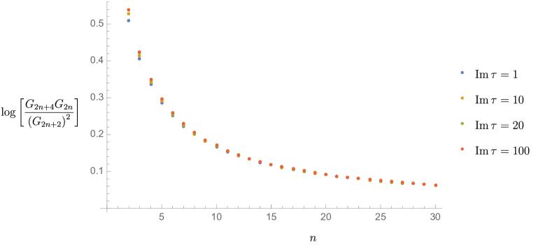
Figure 1: Approximate values of the LHS of sum rule (5.20) in conformal SQCD with $G=SU(2)$ and $N_{f}=4$, calculated via recursion relations from the $S^{4}$ partition function, with instanton corrections omitted.

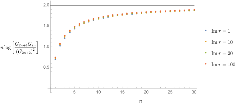
Figure 2: Approximate values of the LHS of sum rule (5.21) in conformal SQCD with $G=SU(2)$ and $N_{f}=4$, calculated via recursion relations from the $S^{4}$ partition function, with instanton corrections omitted.

Figure 3: Approximate values of the LHS of sum rule (5.22) in conformal SQCD with $G=SU(2)$ and $N_{f}=4$, calculated via recursion relations from the $S^{4}$ partition function, with instanton corrections omitted. For the exact $S^{4}$ partition function, with all instanton corrections, our analysis predicts the LHS of (5.22) should approach $-4$ for any $\tau$, as $n$ goes to infinity. It would appear unlikely that the asymptotic value of of the sum rule is truly $-4$ for the no-instanton approximation to the $S^{4}$ partition function, but at present the authors have no theory of the error.

6 Conclusions

Other theories with one-dimensional Coulomb branch

There are many other theories with one dimensional Coulomb branch (or more generally with a single vector multiplet and massless hypers) without marginal coupling. Since these do not have marginal couplings, they are harder to do explicit calculations with and we do not have results in the literature with which we can easily compare. In order to predict correlation functions of $({\cal O})^{n}$ for large $n$, we must know the dimension of the generator ${\cal O}$, the $a$-coefficient of the full CFT, and the massless content of the effective theory on moduli space.

Rank-one SCFT have been the subject of intensive recent study by [6, 7, 8, 9], in which theories with one-dimensional Coulomb branch were classified under broad conditions.

We make use of the beautiful results [8, 9, 7, 6] on the classification of rank-one superconformal field theories. Actually we will do more than just "make use of" them: Table 1 is created by copying directly a table from [8], but with our our own additional columns, giving data on the Wess–Zumino term and the value of the $\alpha$-coefficient of the theory.

$\begin{array}[]{clc|c|c|cc||cc|c}\hline\cr&\lx@intercol\text{Coulomb branch:}\hfil\lx@intercol\vrule\lx@intercol&\text{higgs}&\lx@intercol\text{massless}\hfil\lx@intercol\vrule\lx@intercol&\lx@intercol\text{Central charges:}\hfil\lx@intercol\vrule\lx@intercol\vrule\lx@intercol&\lx@intercol\text{Wess-Zumino term:}\hfil\lx@intercol\vrule\lx@intercol&\lx@intercol\text{$\alpha$-coefficient:}\hfil\lx@intercol\\[2.84526pt] &\text{${{\rm singul.}\atop{\rm type}}$}&\Delta_{\cal O}&\text{br. dim}&{\rm hypers}&\ \ 24a&\ \ 12c&\ \ 24a_{{\rm EFT}}{}&\ \ 24\Delta a&\ \ \alpha=2\Delta a\\[4.2679pt] \hline\cr\hline\cr&&&&&&&&&\\[-12.80373pt] &II^{*}&6&29&0&95&62&5&90&15/2\\ &III^{*}&4&17&0&59&38&5&54&9/2\\ &IV^{*}&3&11&0&41&26&5&36&3\\ &I_{0}^{*}&2&5&0&23&14&5&18&3/2\\ &IV&3/2&2&0&14&8&5&9&3/4\\ &III&4/3&1&0&11&6&5&6&1/2\\ &II&6/5&0&0&43/5&22/5&5&18/5&3/10\\ \hbox{\multirowsetup\begin{sideways}$I_{1}$ series\qquad\ \end{sideways}}&I_{1}&1&0&0&6&3&5&1&1/12\\[1.42262pt] \hline\cr\hline\cr&&&&&&&&&\\[-12.80373pt] &II^{*}&6&16&5&82&49&10&72&6\\ &III^{*}&4&8&3&50&29&8&42&7/2\\ &IV^{*}&3&4&2&34&19&7&27&9/4\\ &{\color[rgb]{0,0,1}{I_{0}^{*}}}&2&0&1&18&9&6&12&1\\ \hbox{\multirowsetup\begin{sideways}$I_{4}$ series\qquad\ \end{sideways}}&I_{4}&1&0&0&6&3&5&1&1/12\\[1.42262pt] \hline\cr\hline\cr&&&&&&&&&\\[-12.80373pt] &II^{*}&6&9&4&75&42&9&66&11/2\\ &III^{*}&4&?&2&45&24&7&38&19/6\\ &{\color[rgb]{1,0,0}{IV^{*}}}&3&0&1&30&15&6&24&2\\ \hbox{\multirowsetup\begin{sideways}$I_{1}^{*}$ series\qquad\ \end{sideways}}&I_{1}^{*}&2&0&0&17&8&5&12&1\\[1.42262pt] \hline\cr\hline\cr&&&&&&&&&\\[-12.80373pt] &II^{*}&6&?&3&71&38&8&63&21/4\\ &{\color[rgb]{1,0,0}{III^{*}}}&4&0&1&42&21&6&36&3\\ \hbox{\multirowsetup\begin{sideways}$\scriptstyle{IV^{*}_{\scriptscriptstyle Q=1}}$ \small{ser.}\quad\ \end{sideways}}&IV^{*}_{Q=1}&3&0&0&55/2&25/2&5&45/2&9/4\\[1.42262pt] \hline\cr\hline\cr&&&&&&&&&\\[-12.80373pt] &{\color[rgb]{0,0,1}{I_{0}^{*}}}&2&0&1&18&9&6&12&1\\ \hbox{\multirowsetup\begin{sideways}$I_{2}$ ser.\quad\ \ \end{sideways}}&I_{2}&1&0&0&6&3&5&1&1/12\\[1.42262pt] \hline\cr\hline\cr\end{array}$

Table 1: Argyres, Lotito, Lu and Martone’s partial list of rank-1 ${\cal N}=2$ SCFTs. This table has been copied directly (at the level of the LaTEX code even) from [8], to clarify the identification of theories, which are labelled exactly as in that reference. We have added the three columns on the right, including the $\alpha$-coefficient. The column ‘massless hypers’ denotes the number of hypermultiplets massless at a generic point on the Coulomb branch, a situation referred to in [8] as an ‘enhanced Coulomb branch’ (ECB) if the number is nonzero.

Conclusions

In this paper we have analyzed the large-quantum-number expansion of two-point functions of operators ${\cal O}_{\Delta}^{n}$, where ${\cal O}_{\Delta}$ is the holomorphic generator of a Coulomb branch chiral ring in a rank-one superconformal field theory. To do this, we have followed earlier works and used the effective field theory governing the large-${{\color[rgb]{.54,.17,.888}{{\cal J}}}}$ sector of the Hilbert space. As in the previous paper [1] on the superconformal large-${{\color[rgb]{.54,.17,.888}{{\cal J}}}}$ expansion, the relevant EFT is the effective dynamics of the supersymmetric moduli space, which is governed by spontaneously broken superconformal symmetry. We have used the Coulomb-branch EFT to expand the two-point function

$$\begin{split}{\cal Y}_{n}\equiv|x-y|^{2{{\color[rgb]{.54,.17,.888}{{\cal J}}}}}\,\left<({\cal O}(x))^{n}\,(\bar{{\cal O}}(y))^{n}\right>\end{split}$$

at large $R$-charge, i.e., for $n\gg 1$. The EFT predicts that ${\cal Y}_{n}$ has an asymptotic expansion at large $n$, behaving as

$$\begin{split}{\cal Y}_{n}=({{\color[rgb]{.54,.17,.888}{{\cal J}}}})!\,\left({{|{\bf N}_{\cal O}|}\over{2\pi}}\right)^{2{{\color[rgb]{.54,.17,.888}{{\cal J}}}}}\,{{\color[rgb]{.54,.17,.888}{{\cal J}}}}^{\alpha}\,\tilde{{\cal Y}}_{n}\ ,\end{split}$$

where $\tilde{{\cal Y}}_{n}$ approaches a constant as $n\to\infty$, and ${\bf N}_{\cal O}$ is an $n$-independent constant depending on the normalization of the operator relative to the effective Abelian gauge coupling $g_{{\rm eff}}{}$. We have calculated the exponent $\alpha$ and found that it is computed entirely by the coupling between the Euler density of the sphere and the logarithm of the scalar modulus $|\phi|$. This coupling is fixed by anomaly matching to be proportional to the difference between the $a$-anomaly coefficient of the underlying CFT and that of the EFT of massless moduli. In the conventions of [50], this is

$$\begin{split}\alpha=2\,\left(a_{{\rm CFT}}{}-a_{{\rm EFT}}{}\right)^{\rm[AEFJ]}\ .\end{split}$$

In theories with a marginal coupling, we have used results from localization [2, 3, 4, 5] to test our predictions. In the case of ${\cal N}=4$ SYM with gauge group $SU(2)$ (or more properly gauge algebra $\mathfrak{su}(2)$ in general), the exact result can be expressed in closed form, and our asymptotic expansion for the logarithm of the two point function agrees precisely with the exact result to the precision to which we have calculated, i.e. up to and including the order $\log({{\color[rgb]{.54,.17,.888}{{\cal J}}}})$ term in ${\cal B}_{n}=\log({\cal Y}_{n})$. In the case of superconformal SQCD with $N_{f}=2N_{c}=4$, we compare our large-${{\color[rgb]{.54,.17,.888}{{\cal J}}}}$ expansion with the output of the recursion relations carried to ${{\color[rgb]{.54,.17,.888}{{\cal J}}}}\simeq 60$, with the ${{\color[rgb]{.54,.17,.888}{{\cal J}}}}=0$ expression approximated by the zero-instanton part of the $S^{4}$ partition function. We find precise numerical agreement for the two leading-order behaviors, and good agreement for the sub-subleading order behavior, dictated by the $\alpha$-coefficient $\alpha=+{3\over 2}$, which predicts a value $-4$ for the LHS of the sum rule (5.22) at large $n$. Though it is not clear we should expect the sum rule to approach $-4$ precisely for the zero-instanton approximation to the initial condition $Z_{S^{4}}$, the sum rule for $\tau=i$ appears to asymptote to a value at most $\simeq-3.8$, to within our numerical precision. It would be desirable to have a robust theory of the error at large ${{\color[rgb]{.54,.17,.888}{{\cal J}}}}$, given an approximate initial condition for the recursion relation. It may be a useful direction to study the recursion relations directly in a ${1\over{{\color[rgb]{.54,.17,.888}{{\cal J}}}}}$ expansion, to understand to what extent the large-${{\color[rgb]{.54,.17,.888}{{\cal J}}}}$ behavior is determined by initial condition $Z_{S^{4}}(\tau,{\bar{\tau}})$ and to what extent it is guided by attractor phenomena inherent to the recursion relations themselves.

In summary, we have shown that it is practical to use the large-${{\color[rgb]{.54,.17,.888}{{\cal J}}}}$ expansion as a bridge from the world of unbroken conformal symmetry, OPE data, and bootstraps, to the world of the low-energy dynamics of the moduli space of vacua.

Appendix A Normalizations and conventions

A.1 Massless scalar propagator

Define the free massless complex scalar field $\phi_{{\rm unit}}{}$ to have kinetic term

$$\begin{split}{\cal L}=+1\,|\partial\phi_{{\rm unit}}{}|^{2}\ ,\end{split}$$ (A.1)

in Euclidean signature, where $\partial^{2}\equiv\partial_{\mu}\partial_{\mu}$ and $|\partial\phi|^{2}\equiv(\partial_{\mu}\phi)(\partial_{\mu}{\bar{\phi}})$. The massless euclidean scalar propagator on ${\mathbb{R}}^{4}$ is defined as

$$\begin{split}\Delta_{{\rm unit}}{}(x,y)\equiv\left<\phi_{{\rm unit}}{}(x)\,\,{\bar{\phi}}_{{\rm unit}}{}(y)\right>_{{\mathbb{R}}^{4}}\ .\end{split}$$ (A.2)

Given (A.1), the Ward identity yields the equation of motion for the propagator

$$\begin{split}\partial_{x}^{2}\Delta_{{\rm unit}}{}(x,y)=\partial_{y}^{2}\Delta_{{\rm unit}}{}(x,y)=-\delta^{({4})}(x-y)\end{split}$$ (A.3)

so the propagator for the unit scalar has normalization

$$\begin{split}\Delta_{{\rm unit}}{}(x,y)=+(2\pi)^{-2}\,|x-y|^{-2}\end{split}$$ (A.4)

where we have used the identity

$$\begin{split}\partial^{2}_{x}\left|x-y\right|^{-2}=-(2\pi)^{2}\delta^{(4)}(x-y)\end{split}$$ (A.5)

on ${\mathbb{R}}^{4}$. More generally, for a massless complex scalar field normalized as

$$\begin{split}{\cal L}_{\bf M}^{2}={\bf M}^{2}\,|\partial_{\mu}\phi|^{2}\ ,\end{split}$$ (A.6)

the scalar propagator is

$$\begin{split}\left<\phi(x)\,{\bar{\phi}}(y)\right>_{{\mathbb{R}}^{4}}=(2\pi)^{-2}\,{\bf M}^{-2}\,|x-y|^{-2}\end{split}$$ (A.7)

for any positive real ${\bf M}$. In particular, for the $A$-field of the effective Abelian vector multiplet, whose kinetic term is (2.8), the two-point function is

$$\begin{split}\left<A(x)\,\bar{A}(y)\right>_{{\mathbb{R}}^{4}}={{g^{2}_{{\rm eff}}{}}\over{(2\pi)^{2}}}\,|x-y|^{-2}={1\over{\pi\,{\rm Im}(\tau)}}\,|x-y|^{-2}.\end{split}$$ (A.8)

A.2 Geometry of the four-sphere

The four-sphere is a symmetric space, so its Riemann tensor satisfies

$$\begin{split}R_{abcd}={1\over{r^{2}}}(g_{ac}g_{bd}-g_{ad}g_{bc})\ .\end{split}$$ (A.9)

So for a general $D$-dimensional sphere we have

$$\begin{split}R_{ac}=g^{bd}R_{abcd}={1\over{r^{2}}}\,(D-1)g_{ac}\ ,\qquad R=g^{ac}R_{ac}={{D(D-1)}\over{r^{2}}}\ .\end{split}$$ (A.10)

Now let us calculate the Euler density, according to Komargodski-Schwimmer’s normalization convention (4.6). The square of the Riemann tensor is

$$\begin{split}R_{abcd}^{2}\equiv g^{aa^{\prime}}g^{bb^{\prime}}g^{cc^{\prime}}g^{dd^{\prime}}\,R_{abcd}R_{a^{\prime}b^{\prime}c^{\prime}d^{\prime}}=2\,{{D(D-1)}\over{r^{4}}}\end{split}$$ (A.11)

and the squares of the Ricci tensor and Ricci scalar are

$$\begin{split}R_{ab}={{D-1}\over{r^{2}}}\,g_{ab}\ ,\qquad R_{ab}^{2}\equiv g^{ac}g^{bd}R_{ab}R_{cd}={{D(D-1)^{2}}\over{r^{4}}}\ .\end{split}$$ (A.12)

The Ricci scalar and its square are

$$\begin{split}R={{D(D-1)}\over{r^{2}}}\ ,\qquad R^{2}={{D^{2}(D-1)^{2}}\over{r^{4}}}\ .\end{split}$$ (A.13)

The case of interest to us is $D=4$, in which

$$\begin{split}(R_{abcd}^{2})_{D=4}={{24}\over{r^{4}}}\ ,\qquad(R_{ab}^{2})_{D=4}={{36}\over{r^{4}}}\ ,\qquad(R^{2})_{D=4}={{144}\over{r^{4}}}\ .\end{split}$$ (A.14)

Komargodski-Schwimmer’s normalization of the Euler density, in their equation (A.4), is

$$\begin{split}E_{4}^{\rm[KS]}\equiv R_{abcd}^{2}-4R_{ab}^{2}+R^{2}\ ,\end{split}$$ (A.15)

which for the four-sphere of radius $r$, is given by

$$\begin{split}E_{4}^{\rm[KS]}={{24}\over{r^{4}}}\ .\end{split}$$ (A.16)

A.3 Conventions and values for the $a$-anomaly coefficient

In this part of the Appendix, we compare two conventions for the normalization of the $a$-anomaly coefficient (also the $c$-anomaly coefficient), and we give values for the anomaly in various ${\cal N}=2$ SCFT of interest. We also give a definition of the $\alpha$-coefficient that is independent of the normalization of the $a$-anomaly.

Translation between Weyl-anomaly normalization conventions in [68] vs. [50]

The $a$- and $c$-anomalies are normalized differently in different parts of the literature. We can match by comparing anomalies for a given physical system across conventions. The simplest case is a scalar field.

In [68] the anomalies are normalized so that the contributions of a single real massless scalar field, are

$$\begin{split}a^{\rm[KS]}_{\text{real massless scalar}}=\frac{1}{90(8\pi)^{2}}\ ,\qquad c^{\rm[KS]}_{\text{real massless scalar}}=\frac{1}{30(8\pi)^{2}}\ .\end{split}$$ (A.17)

This normalization is given below equation (A.6) of [68]. In [50], the authors give the anomalies of a single real massless scalar field, as

$$\begin{split}a^{\rm[AEFJ]}_{\text{real massless scalar}}=\frac{1}{360}\ ,\qquad c^{\rm[AEFJ]}_{\text{real massless scalar}}=\frac{1}{120}\ .\end{split}$$ (A.18)

The relation between the two normalizations is therefore

$$\begin{split}a^{\rm[KS]}={1\over{16\pi^{2}}}\,a^{\rm[AEFJ]}\ ,\qquad c^{\rm[KS]}={1\over{16\pi^{2}}}\,c^{\rm[AEFJ]}.\end{split}$$ (A.19)

In the body of the paper we indicate our conventions to avoid ambiguity, but we shall use the convention of [50], since it is normalized such that the anomalies of free fields, and of all ${\cal N}=2$ SCFT, are rational numbers.

Values of the anomaly coefficient in various ${\cal N}=2$ SCFT in $D=4$

We have defined the exponent $\alpha$, which appears in the factor ${{\color[rgb]{.54,.17,.888}{{\cal J}}}}^{\alpha}$ in the asymptotic formula for the two-point function, in terms of the $a$ coefficient in the Weyl anomaly. The Weyl anomaly does not have a universally used normalization in the literature. So in order to find actual values for $\alpha$, we need to use some particular conventions.

The $a$-coefficients for many Lagrangian and non-Lagrangian theories, have been given in e.g. [50, 76], and we collect the relevant results here. Those authors normalize the $a$-coefficient according to the widely-used convention in [50], in which we have

$$\begin{split}a_{\rm favm}^{\rm[AEFJ]}={5\over{24}},\quad a_{\rm fhm}^{\rm[AEFJ]}={1\over{24}}\ ,\quad a_{{\rm vm}_{G}}^{\rm[AEFJ]}={5\over{24}}\,\dim(G)\ ,\quad a_{{\rm hm}_{R}}^{\rm[AEFJ]}={1\over{24}}\,\dim_{\mathbb{C}}(R)\ .\end{split}$$ (A.20)

Value of the $a$-coefficient for ${\cal N}=4$ SYM

Organizing into ${\cal N}=4$ vectormultiplets, we have

$$\begin{split}a_{{\cal N}=4\rm~{}favm}^{\rm[AEFJ]}=a_{\rm favm}^{\rm[AEFJ]}+a_{\rm fhm}^{\rm[AEFJ]}=\frac{1}{4}\ ,\qquad a^{\rm[AEFJ]}_{{\cal N}=4\rm~{}vm_{G}}={1\over 4}\,\dim(G)\ .\end{split}$$ (A.21)

The ${\cal N}=4$ theory with gauge group $G$ has microscopic $a$-coefficient

$$\begin{split}a^{\rm[AEFJ]}_{{\rm CFT,~{}{\cal N}=4}}{}={1\over 4}\,\dim(G)\end{split}$$ (A.22)

and its moduli space effective theory has

$$\begin{split}a^{\rm[AEFJ]}_{{\rm EFT,~{}{\cal N}=4}}{}={1\over 4}\,\operatorname{\mathop{rank}}(G)\end{split}$$ (A.23)

so

$$\begin{split}\Delta a^{\rm[AEFJ]}_{{\rm{\cal N}=4}}{}={1\over 4}\,\left(\,\dim(G)-\operatorname{\mathop{rank}}(G)\,\right)\ .\end{split}$$ (A.24)

For $SU(N_{c})$ gauge group, we have

$$\begin{split}\Delta a^{\rm[AEFJ]}_{{\cal N}=4,~{}G=SU(N_{c})}={1\over 4}(N_{c}^{2}-N_{c})\ .\end{split}$$ (A.25)

In particular, for $N_{c}=2$ we have

$$\begin{split}\Delta a^{\rm[AEFJ]}_{{\cal N}=4,~{}G=SU(2)}=\frac{1}{2}.\end{split}$$ (A.26)

Value of the $a$-coefficient for superconformal ${\cal N}=2$ SQCD

For ${\cal N}=2$ SQCD with gauge group $SU(N_{c})$ and $N_{f}$ fundamental flavors at weak coupling, we have

$$\begin{split}a^{\rm[AEFJ]}_{{\rm UV,~{}SQCD}}{}={5\over{24}}\,\dim(G)+{1\over{24}}\,\dim_{\mathbb{C}}(R)={5\over{24}}(N_{c}^{2}-1)+{1\over{24}}\,N_{f}N_{c}\ .\end{split}$$ (A.27)

In the superconformal case, $N_{f}=2N_{c}$ we have

$$\begin{split}a^{\rm[AEFJ]}_{{\rm CFT,~{}SCQCD}}{}={5\over{24}}\,\dim(G)+{1\over{24}}\,\dim_{\mathbb{C}}(R)={5\over{24}}(N_{c}^{2}-1)+{1\over{12}}\,N_{c}^{2}={7\over{24}}\,N_{c}^{2}-{5\over{24}}\ .\end{split}$$ (A.28)

The moduli space effective theory consists of $\operatorname{\mathop{rank}}(G)$ free abelian vector multiplets and no hypers, so we have

$$\begin{split}a^{\rm[AEFJ]}_{{\rm EFT,~{}SCQCD}}{}={5\over{24}}\,\operatorname{\mathop{rank}}(G)\ ,\end{split}$$ (A.29)

which for $G=SU(N)$, is

$$\begin{split}a^{\rm[AEFJ]}_{{\rm EFT,~{}SCQCD}}{}={5\over{24}}\,(N_{c}-1)\ .\end{split}$$ (A.30)

So the difference in central charge is

$$\begin{split}\Delta a^{\rm[AEFJ]}_{{\rm SCQCD}}{}=a^{\rm[AEFJ]}_{{\rm CFT,~{}SCQCD}}{}-a^{\rm[AEFJ]}_{{\rm EFT,~{}SCQCD}}{}={1\over{24}}\,\left(\,7N_{c}^{2}-5N_{c}\,\right)\ .\end{split}$$ (A.31)

Value of the $\alpha$-coefficient for ${\cal N}=4$ SYM

So for ${\cal N}=4$ we have

$$\begin{split}\alpha_{{\cal N}=4}={1\over 2}\,(N_{c}^{2}-N_{c})\ .\end{split}$$ (A.32)

In particular, for $G=SU(2)$ we have

$$\begin{split}\alpha_{{\cal N}=4,~{}G=SU(2)}=+1\ .\end{split}$$ (A.33)

Value of the $\alpha$-coefficient for ${\cal N}=2$ superconformal SQCD

For superconformal QCD (that is, $N_{f}=2N_{c}$), we have

$$\begin{split}\alpha_{{\rm SCQCD}}={1\over{12}}\,\left(\,7N_{c}^{2}-5N_{c}\,\right)\ ,\end{split}$$ (A.34)

and in particular for $G=SU(2)$ with $N_{f}=2N_{c}=4$, we have

$$\begin{split}\alpha_{{\rm SCQCD},~{}G=SU(2)}=\frac{3}{2}\end{split}$$ (A.35)

Convention-independent formula for the $\alpha$-coefficient

We would like to define the $\alpha$-coefficient in a convention-independent way, as a ratio of $a$-anomalies. Our convention-independent formula is:

$$\begin{split}\alpha={5\over{12}}\,{{a_{{\rm CFT}}{}-a_{{\rm EFT}}{}}\over{a_{{\rm favm}}{}}}\ ,\end{split}$$ (A.36)

where $a_{{\rm favm}}{}$ is the unit of $a$-anomaly contribution carried by a free ${\cal N}=2$ vector multiplet for a $U(1)$ gauge group. In order to actually compute the value of $\alpha$ for some theories of interest, we must pick an actual normalization convention. The value of $\alpha$ in the [50] convention is

$$\begin{split}\alpha=2\,\left(\,a^{\rm[AEFJ]}_{{\rm CFT}}{}-a^{\rm[AEFJ]}_{{\rm EFT}}{}\,\right)\ ,\end{split}$$ (A.37)

and in the [68] convention it is

$$\begin{split}\alpha={1\over{8\pi^{2}}}\,\left(\,a^{\rm[KS]}_{{\rm CFT}}{}-a^{\rm[KS]}_{{\rm EFT}}{}\,\right)\ .\end{split}$$ (A.38)

References

- [1] S. Hellerman, S. Maeda, and M. Watanabe, "Operator Dimensions from Moduli," JHEP 10 (2017) 89, arXiv:1706.05743 [hep-th].
- [2] M. Baggio, V. Niarchos, and K. Papadodimas, " equations, localization and exact chiral rings in 4d =2 SCFTs," JHEP 02 (2015) 122, arXiv:1409.4212 [hep-th].
- [3] M. Baggio, V. Niarchos, and K. Papadodimas, "Exact correlation functions in superconformal QCD," Phys. Rev. Lett. 113 no. 25, (2014) 251601, arXiv:1409.4217 [hep-th].
- [4] M. Baggio, V. Niarchos, and K. Papadodimas, "On exact correlation functions in superconformal QCD," JHEP 11 (2015) 198, arXiv:1508.03077 [hep-th].
- [5] E. Gerchkovitz, J. Gomis, N. Ishtiaque, A. Karasik, Z. Komargodski, and S. S. Pufu, "Correlation Functions of Coulomb Branch Operators," JHEP 01 (2017) 103, arXiv:1602.05971 [hep-th].
- [6] P. Argyres, M. Lotito, Y. Lu, and M. Martone, "Geometric constraints on the space of N=2 SCFTs I: physical constraints on relevant deformations," arXiv:1505.04814 [hep-th].
- [7] P. C. Argyres, M. Lotito, Y. Lu, and M. Martone, "Geometric constraints on the space of N=2 SCFTs II: Construction of special Kahler geometries and RG flows," arXiv:1601.00011 [hep-th].
- [8] P. Argyres, M. Lotito, Y. Lu, and M. Martone, "Geometric constraints on the space of N=2 SCFTs III: enhanced Coulomb branches and central charges," arXiv:1609.04404 [hep-th].
- [9] P. C. Argyres, M. Lotito, Y. Lu, and M. Martone, "Expanding the landscape of = 2 rank 1 SCFTs," JHEP 05 (2016) 088, arXiv:1602.02764 [hep-th].
- [10] S. Hellerman, D. Orlando, S. Reffert, and M. Watanabe, "On the CFT Operator Spectrum at Large Global Charge," JHEP 12 (2015) 071, arXiv:1505.01537 [hep-th].
- [11] L. Alvarez-Gaume, O. Loukas, D. Orlando, and S. Reffert, "Compensating strong coupling with large charge," JHEP 04 (2017) 059, arXiv:1610.04495 [hep-th].
- [12] A. Monin, D. Pirtskhalava, R. Rattazzi, and F. K. Seibold, "Semiclassics, Goldstone Bosons and CFT data," JHEP 06 (2017) 011, arXiv:1611.02912 [hep-th].
- [13] O. Loukas, "Abelian scalar theory at large global charge," Fortsch. Phys. 65 no. 9, (2017) 1700028, arXiv:1612.08985 [hep-th].
- [14] S. Hellerman, N. Kobayashi, S. Maeda, and M. Watanabe, "A Note on Inhomogeneous Ground States at Large Global Charge," arXiv:1705.05825 [hep-th].
- [15] O. Loukas, D. Orlando, and S. Reffert, "Matrix models at large charge," JHEP 10 (2017) 085, arXiv:1707.00710 [hep-th].
- [16] D. Banerjee, S. Chandrasekharan, and D. Orlando, "Conformal dimensions via large charge expansion," arXiv:1707.00711 [hep-lat].
- [17] A. L. Fitzpatrick, J. Kaplan, D. Poland, and D. Simmons-Duffin, "The Analytic Bootstrap and AdS Superhorizon Locality," JHEP 12 (2013) 004, arXiv:1212.3616 [hep-th].
- [18] Z. Komargodski and A. Zhiboedov, "Convexity and Liberation at Large Spin," JHEP 11 (2013) 140, arXiv:1212.4103 [hep-th].
- [19] D. Li, D. Meltzer, and D. Poland, "Conformal Collider Physics from the Lightcone Bootstrap," JHEP 02 (2016) 143, arXiv:1511.08025 [hep-th].
- [20] D. Li, D. Meltzer, and D. Poland, "Non-Abelian Binding Energies from the Lightcone Bootstrap," JHEP 02 (2016) 149, arXiv:1510.07044 [hep-th].
- [21] A. Kaviraj, K. Sen, and A. Sinha, "Analytic bootstrap at large spin," JHEP 11 (2015) 083, arXiv:1502.01437 [hep-th].
- [22] A. Kaviraj, K. Sen, and A. Sinha, "Universal anomalous dimensions at large spin and large twist," JHEP 07 (2015) 026, arXiv:1504.00772 [hep-th].
- [23] P. Dey, K. Ghosh, and A. Sinha, "Simplifying large spin bootstrap in Mellin space," arXiv:1709.06110 [hep-th].
- [24] L. F. Alday and A. Zhiboedov, "An Algebraic Approach to the Analytic Bootstrap," JHEP 04 (2017) 157, arXiv:1510.08091 [hep-th].
- [25] L. F. Alday, "Large Spin Perturbation Theory," Phys. Rev. Lett. 119 no. 11, (2017) 111601, arXiv:1611.01500 [hep-th].
- [26] L. F. Alday, "Solving CFTs with Weakly Broken Higher Spin Symmetry," arXiv:1612.00696 [hep-th].
- [27] S. Hellerman and I. Swanson, "Boundary Operators in Effective String Theory," JHEP 04 (2017) 085, arXiv:1609.01736 [hep-th].
- [28] S. Hellerman, S. Maeda, J. Maltz, and I. Swanson, "Effective String Theory Simplified," JHEP 09 (2014) 183, arXiv:1405.6197 [hep-th].
- [29] S. Hellerman and I. Swanson, "String Theory of the Regge Intercept," Phys. Rev. Lett. 114 no. 11, (2015) 111601, arXiv:1312.0999 [hep-th].
- [30] M. S. Costa, V. Goncalves, and J. Penedones, "Conformal Regge theory," JHEP 12 (2012) 091, arXiv:1209.4355 [hep-th].
- [31] S. Caron-Huot, Z. Komargodski, A. Sever, and A. Zhiboedov, "Strings from Massive Higher Spins: The Asymptotic Uniqueness of the Veneziano Amplitude," JHEP 10 (2017) 026, arXiv:1607.04253 [hep-th].
- [32] A. Sever and A. Zhiboedov, "On Fine Structure of Strings: The Universal Correction to the Veneziano Amplitude," arXiv:1707.05270 [hep-th].
- [33] D. T. Son and M. Wingate, "General coordinate invariance and conformal invariance in nonrelativistic physics: Unitary Fermi gas," Annals Phys. 321 (2006) 197–224, arXiv:cond-mat/0509786 [cond-mat].
- [34] R. Rattazzi, V. S. Rychkov, E. Tonni, and A. Vichi, "Bounding scalar operator dimensions in 4D CFT," JHEP 12 (2008) 031, arXiv:0807.0004 [hep-th].
- [35] S. El-Showk, M. F. Paulos, D. Poland, S. Rychkov, D. Simmons-Duffin, and A. Vichi, "Solving the 3d Ising Model with the Conformal Bootstrap II. -Minimization and Precise Critical Exponents," J. Stat. Phys. 157 (2014) 869, arXiv:1403.4545 [hep-th].
- [36] S. El-Showk, M. F. Paulos, D. Poland, S. Rychkov, D. Simmons-Duffin, and A. Vichi, "Solving the 3D Ising Model with the Conformal Bootstrap," Phys. Rev. D86 (2012) 025022, arXiv:1203.6064 [hep-th].
- [37] S. Rychkov, "EPFL Lectures on Conformal Field Theory in Dimensions," SpringerBriefs in Physics (2016) , arXiv:1601.05000 [hep-th].
- [38] D. Simmons-Duffin, "The Conformal Bootstrap," Proceedings, Theoretical Advanced Study Institute in Elementary Particle Physics: New Frontiers in Fields and Strings (TASI 2015): Boulder, CO, USA, June 1-26, 2015 (2017) 1–74, arXiv:1602.07982 [hep-th].
- [39] M. Srednicki, "Chaos and quantum thermalization," Phys. Rev. E50 (1994) 888–901, arXiv:cond-mat/9403051 [cond-mat].
- [40] D. Jafferis, B. Mukhametzhanov, and A. Zhiboedov, "Conformal Bootstrap At Large Charge," arXiv:1710.11161 [hep-th].
- [41] A. Zhiboedov, "Conformal Bootstrap At Large Charge," MS seminar at Kavli Institute for the Physics and Mathematics of the Universe. Oct., 2017. http://research.ipmu.jp/seminar/?seminar_id=1939.
- [42] D. Rodriguez-Gomez and J. G. Russo, "Large Correlation Functions in Superconformal Field Theories," JHEP 06 (2016) 109, arXiv:1604.07416 [hep-th].
- [43] M. Dedushenko, S. S. Pufu, and R. Yacoby, "A one-dimensional theory for Higgs branch operators," arXiv:1610.00740 [hep-th].
- [44] M. Baggio, V. Niarchos, K. Papadodimas, and G. Vos, "Large-N correlation functions in = 2 superconformal QCD," JHEP 01 (2017) 101, arXiv:1610.07612 [hep-th].
- [45] A. Pini, D. Rodriguez-Gomez, and J. G. Russo, "Large correlation functions in 2 superconformal quivers," JHEP 08 (2017) 066, arXiv:1701.02315 [hep-th].
- [46] M. Baggio, V. Niarchos, and K. Papadodimas, "Aspects of Berry phase in QFT," JHEP 04 (2017) 062, arXiv:1701.05587 [hep-th].
- [47] M. Billo, F. Fucito, A. Lerda, J. F. Morales, Ya. S. Stanev, and C. Wen, "Two-point Correlators in Gauge Theories," arXiv:1705.02909 [hep-th].
- [48] N. B. Agmon, S. M. Chester, and S. S. Pufu, "A New Duality Between Superconformal Field Theories in Three Dimensions," arXiv:1708.07861 [hep-th].
- [49] K. Papadodimas, "Topological Anti-Topological Fusion in Four-Dimensional Superconformal Field Theories," JHEP 08 (2010) 118, arXiv:0910.4963 [hep-th].
- [50] D. Anselmi, J. Erlich, D. Z. Freedman, and A. A. Johansen, "Positivity Constraints on Anomalies in Supersymmetric Gauge Theories," Phys. Rev. D57 (1998) 7570–7588, arXiv:hep-th/9711035 [hep-th].
- [51] P. C. Argyres, A. M. Awad, G. A. Braun, and F. P. Esposito, "Higher derivative terms in supersymmetric effective actions," JHEP 07 (2003) 060, arXiv:hep-th/0306118 [hep-th].
- [52] P. C. Argyres, A. M. Awad, G. A. Braun, and F. P. Esposito, "Higher derivative terms in SUSY effective actions," Proceedings, 3rd International Symposium on Quantum theory and symmetries (QTS3): Cincinnati, USA, September 10-14, 2003 (2004) 287–293, arXiv:hep-th/0402203 [hep-th].
- [53] P. C. Argyres, A. M. Awad, G. A. Braun, and F. P. Esposito, "On superspace Chern-Simons-like terms," JHEP 02 (2005) 006, arXiv:hep-th/0411081 [hep-th].
- [54] P. C. Argyres, A. Awad, P. Moomaw, and J. Wittig, "Holomorphic higher-derivative terms in supersymmetric effective actions," Proceedings, 7th International Workshop on Supersymmetries and Quantum Symmetries (SQS’07): Dubna, Russia, July 30 - August 04, 2007 (2008) 267–274. https://inspirehep.net/record/1391563/files/P267.pdf.
- [55] N. Seiberg and E. Witten, "Electric - magnetic duality, monopole condensation, and confinement in supersymmetric Yang-Mills theory," Nucl. Phys. B426 (1994) 19–52, arXiv:hep-th/9407087 [hep-th]. [Erratum: Nucl. Phys. B430, 485 (1994)].
- [56] N. Seiberg and E. Witten, "Monopoles, duality and chiral symmetry breaking in supersymmetric QCD," Nucl. Phys. B431 (1994) 484–550, arXiv:hep-th/9408099 [hep-th].
- [57] V. Pestun, "Localization of gauge theory on a four-sphere and supersymmetric Wilson loops," Commun. Math. Phys. 313 (2012) 71–129, arXiv:0712.2824 [hep-th].
- [58] P. C. Argyres and M. R. Douglas, "New phenomena in supersymmetric gauge theory," Nucl. Phys. B448 (1995) 93–126, arXiv:hep-th/9505062 [hep-th].
- [59] P. C. Argyres, M. R. Plesser, N. Seiberg, and E. Witten, "New superconformal field theories in four-dimensions," Nucl. Phys. B461 (1996) 71–84, arXiv:hep-th/9511154 [hep-th].
- [60] D. Xie, "General Argyres-Douglas Theory," JHEP 01 (2013) 100, arXiv:1204.2270 [hep-th].
- [61] N. Bobev, H. Elvang, and T. M. Olson, "Dilaton effective action with supersymmetry," JHEP 04 (2014) 157, arXiv:1312.2925 [hep-th].
- [62] O. Aharony and E. Karzbrun, "On the effective action of confining strings," JHEP 06 (2009) 012, arXiv:0903.1927 [hep-th].
- [63] O. Aharony, M. Field, and N. Klinghoffer, "The effective string spectrum in the orthogonal gauge," JHEP 04 (2012) 048, arXiv:1111.5757 [hep-th].
- [64] O. Aharony and Z. Komargodski, "The Effective Theory of Long Strings," JHEP 05 (2013) 118, arXiv:1302.6257 [hep-th].
- [65] S. R. Coleman, J. Wess, and B. Zumino, "Structure of phenomenological Lagrangians. 1.," Phys. Rev. 177 (1969) 2239–2247.
- [66] C. G. Callan, Jr., S. R. Coleman, J. Wess, and B. Zumino, "Structure of phenomenological Lagrangians. 2.," Phys. Rev. 177 (1969) 2247–2250.
- [67] S. M. Kuzenko, J. Novak, and G. Tartaglino-Mazzucchelli, "Higher derivative couplings and massive supergravity in three dimensions," JHEP 09 (2015) 081, arXiv:1506.09063 [hep-th].
- [68] Z. Komargodski and A. Schwimmer, "On Renormalization Group Flows in Four Dimensions," JHEP 12 (2011) 099, arXiv:1107.3987 [hep-th].
- [69] A. Schwimmer and S. Theisen, "Spontaneous Breaking of Conformal Invariance and Trace Anomaly Matching," Nucl. Phys. B847 (2011) 590–611, arXiv:1011.0696 [hep-th].
- [70] M. Dine and N. Seiberg, "Comments on higher derivative operators in some SUSY field theories," Phys. Lett. B409 (1997) 239–244, arXiv:hep-th/9705057 [hep-th].
- [71] M. A. Luty, J. Polchinski, and R. Rattazzi, "The -theorem and the Asymptotics of 4D Quantum Field Theory," JHEP 01 (2013) 152, arXiv:1204.5221 [hep-th].
- [72] N. A. Nekrasov, "Seiberg-Witten prepotential from instanton counting," Adv. Theor. Math. Phys. 7 no. 5, (2003) 831–864, arXiv:hep-th/0206161 [hep-th].
- [73] L. F. Alday, D. Gaiotto, and Y. Tachikawa, "Liouville Correlation Functions from Four-dimensional Gauge Theories," Lett. Math. Phys. 91 (2010) 167–197, arXiv:0906.3219 [hep-th].
- [74] E. W. Barnes, "The Theory of the Double Gamma Function," Phil. Trans. Roy. Soc. Lond. A 196 (1901) 265–387.
- [75] I. Aniceto, J. G. Russo, and R. Schiappa, "Resurgent Analysis of Localizable Observables in Supersymmetric Gauge Theories," JHEP 03 (2015) 172, arXiv:1410.5834 [hep-th].
- [76] A. D. Shapere and Y. Tachikawa, "Central charges of superconformal field theories in four dimensions," JHEP 09 (2008) 109, arXiv:0804.1957 [hep-th].